Radiation and relativity

Pre-scriptum (dated 26 June 2020): Some of the relevant illustrations in this post were removed as a result of an attack by the dark force. Too bad, because I liked this post. In any case, despite the removal of the illustrations, you should be able to reconstruct the main story line.

Original post:

Now we are really going to do some very serious analysis: relativistic effects in radiation. Fasten your seat belts please.

The Doppler effect for physical waves traveling through a medium

In one of my post – I don’t remember which one – I wrote about the Doppler effect for sound waves, or any physical wave traveling through a medium. I also said it had nothing to do with relativity. What happens really is that the observer sort of catches up with wave or – the other way around: that he falls back – and, because the velocity of a wave in a medium is always the same (that also has nothing to do with relativity: it’s just a general principle that’s true – always), the frequency of the physical wave will appear to be different. [So that’s why a siren of an ambulance sounds different as it moves past you.] Wikipedia has an excellent article on that – so I’ll refer you to that – but so that article does not say anything – or nothing much – about the Doppler effect when electromagnetic radiation is involved. So that’s what we’ll talk about here. Before we do that, though, let me quickly jot down the formula for the Doppler effect for a physical wave traveling through a medium, so we are clear about the differences between the two ‘Doppler effects’:

In this formula, v_p is the propagation speed of the wave in the medium which – as mentioned above – depends on the medium. Now the source and the receiver will have a velocity with respect to the medium as well (positive or negative – depending on whether they’re moving in the same direction as the wave or not), and so that’s v_r (r for receiver) and v_s(s for source) respectively. So we’re adding speeds here to calculate some relative speed and then we take the ratio. Some people think that’s what relativity theory is all about. It’s not. Everything I’ve written so far is just Galilean relativity – so stuff that’s been known for a thousand years already, if not longer.

Relativity is weird: one aspect of it is length contraction – not often discussed – but the other thing is better known: there is no such thing as absolute time, so when we talk velocities, you need to specify according to whose time?

The Doppler effect for electromagnetic radiation

One thing that’s not relative – and which makes things look somewhat similar to what I wrote above – is that the speed of light is always equal to c. That was the startling fact that came out of Maxwell’s equations (startling because it is not consistent with Galilean relativity: it says that we cannot ‘catch up’ with a light wave!) around which Einstein build all of “new physics”, and so it’s something we use rather matter-of-factly in all that we’ll write below.

In all of the preceding posts about light, I wrote – more than once actually – that the movement of the oscillating charge (i.e. the source of the radiation) along the line of sight did not matter: the only thing that mattered was its acceleration in the xy-plane, which is perpendicular to our line of sight, which we’ll call the z-axis. Indeed, let me remind of you of the two equations defining electromagnetic radiation (see my post on light and radiation about a week ago):

The first formula gives the electromagnetic effect that dominates in the so-called wave zone, i.e. a few wavelengths away from the source – because the Coulomb force varies as the inverse of the square of the distance r, unlike this ‘radiation’ effect, which varies inversely as the distance only (E ∝ 1/r), so it falls off much less rapidly.

Now, that general observation still holds when we’re considering an oscillating charge that is moving towards or away from us with some relativistic speed (i.e. a speed getting close enough to c to produce relativistic length contraction and time dilation effects) but, because of the fact that we need to consider local times, our formula for the retarded time is no longer correct.

Huh? Yes. The matter is quite complicated, and Feynman starts with jotting down the derivatives for the displacement in the x- and y-directions, but I think I’ll skip that. I’ll go for the geometrical picture straight away, which is given below. As said, it’s going to be difficult, but try to hang in here, because it’s necessary to understand the Doppler effect in a correct way (I myself have been fooled by quite a few nonsensical explanations of it in popular books) and, as a bonus, you also get to understand synchrotron radiation and other exciting stuff.

So what’s going on here? Well… Don’t look at the illustration above. We’ll come back at it. Let’s first build up the logic. We’ve got a charge moving vertically – from our point that is (the observer), but also moving in and out of us, i.e. in the z-direction. Indeed, note the arrow pointing to the observer: that’s us! So it could indeed be us looking at electrons going round and round and round – at phenomenal speeds – in a synchrotron indeed – but then one that’s been turned 90 degrees (probably easier for us to just lie down on the ground and look sideways). In any case, I hope you can imagine the situation. [If not, try again.] Now, if that charge was not moving at relativistic speeds (e.g. 0.94c, which is actually the number that Feynman uses for the graph above), then we would not have to worry about ‘our’ time t and the ‘local’ time τ. Huh? Local time? Yes.

We denote the time as measured in the reference frame of the moving charge as τ. Hence, as we are counting t = 1, 2, 3 etcetera, the electron is counting τ = 1, 2, 3 etcetera as it goes round and round and round. If the charge would not be moving at relativistic speeds, we’d do the standard thing and that’s to calculate the retarded acceleration of the charge a'(t) = a(t − r/c). [Remember that we used a prime to mark functions for which we should use a retarded argument and, yes, I know that the term ‘retarded’ sounds a bit funny, but that’s how it is. In any case, we’d have a'(t) = a(t − r/c) – so the prime vanishes as we put in the retarded argument.] Indeed, from the ‘law’ of radiation, we know that the field now and here is given by the acceleration of the charge at the retarded time, i.e. t – r/c. To sum it all up, we would, quite simply, relate t and τ as follows:

τ = t – r/c or, what amounts to the same, t = τ + r/c

So the effect that we see now, at time t, was produced at a distance r at time τ = t − r/c. That should make sense. [Again, if it doesn’t: read again. I can’t explain it in any other way.]

The crucial chain in this rather complicated chain of reasoning comes now. You’ll remember that one of the assumptions we used to derive our ‘law’ of radiation was that the assumption that “r is practically constant.” That does no longer hold. Indeed, that electron moving around in the synchrotron comes in and out at us at crazy speeds (0.94c is a bit more than 280,000 km per second), so r goes up and down too, and the relevant distance is not r but r + z(τ). This means the retardation effect is actually a bit larger: it’s not r/c but [r + z(τ)]/c = r/c + z(τ)/c. So we write:

τ = t – r/c – z(τ)/c or, what amounts to the same, t = τ + r/c + z(τ)/c

Hmm… You’ll say this is rather fishy business. Why would we use the actual distance and not the distance a while ago? Well… I’ll let you mull over that. We’ve got two points in space-time here and so they are separated both by distance as well as time. It makes sense to use the actual distance to calculate the actual separation in time, I’d say. If you’re not convinced, I can only refer you to those complicated derivations that Feynman briefly does before introducing this ‘easier’ geometric explanation. This brings us to the next point. We can measure time in seconds, but also in equivalent distance, i.e. light-seconds: the distance that light (remember: always at absolute speed c) travels in one second, i.e. approximately 299,792,458 meter. It’s just another ‘time unit’ to get used to.

Now that’s what’s being done above. To be sure, we get rid of the constant r/c, which is a constant indeed: that amounts to a shift of the origin by some constant (so we start counting earlier or later). In short, we have a new variable ‘t’ really that’s equal to t = τ + z(τ)/c. But we’re going to count time in meter (well – in units of c meter really), so we will just multiply this and we get:

ct = cτ + z(τ)

Why the different unit? Well… We’re talking relativistic speeds here, don’t we? And so the second is just an inappropriate unit. When we’re finished with this example, we’ll give you an even simpler example: a source just moving in on us, with an equally astronomical speed, so the functional shape of z(τ) will be some fraction of c (let’s say kc) times τ, so kcτ. So, to simplify things, just think of it as re-scaling the time axis in units that makes sense as compared to the speeds we are talking about.

Now we can finally analyze that graph on the right-hand side. If we would keep r fixed – so if we’d not care about the charge moving in and out of – the plot of x'(t) – i.e. the retarded position indeed – against ct would yield the sinusoidal graph plotted by the red numbers 1 to 13 here. In fact, instead of a sinusoidal graph, it resembles a normal distribution, but that’s just because we’re looking at one revolution only. In any case, the point to note is that – when everything is said and done – we need to calculate the retarded acceleration, so that’s the second derivative of x'(t). The animated illustration shows how that works: the second derivative (not the first) turns from positive to negative – and vice versa – at inflection points, when the curve goes from convex to concave, and vice versa. So, on the segment of that sinusoidal function marked by the red numbers, it’s positive at first (the slope of the tangent becomes steeper and steeper), then negative (cf. that tangent line turning from blue to green in the illustration below), and then it becomes positive again, as the negative slope becomes less negative at the second inflection point.

That should be straightforward. However, the actual x'(t) curve is the black curve with the cusp. A curve like that is called a hypocycloid. Let me reproduce it once again for ease of reference.

We relate x'(t) to ct (this is nothing but our new unit for t) by noting that ct = cτ + z(τ). Capito? It’s not easy to grasp: the instinct is to just equate t and τ and write x'(t) = x'(τ), but that would not be correct. No. We must measure in ‘our’ time and get a functional form for x’ as a function of t, not of τ. In fact, x'(t) − i.e. the retarded vertical position at time t – is not equal to x'(τ) but to x(τ), i.e. that’s the actual (instead of retarded) position at (local) time τ, and so that’s what the black graph above shows.

I admit it’s not easy. I myself am not getting it in an ‘intuitive’ way. But the logic is solid and leads us where it leads us. Perhaps it helps to think in terms of the curvature of this graph. In fact, we have to think in terms of curvature of this graph in order to understand what’s happening in terms of radiation. When the charge is moving away from us, i.e. during the first three ‘seconds’ (so that’s the 1-2-3 count), we see that the curvature is less than than what it would be – and also doesn’t change very much – if the displacement was given by the sinusoidal function, which means there’s very little radiation (because there’s little acceleration – negative or positive. However, as the charge moves towards us, we get that sharp cusp and, hence, we also get sharp curvature, which results in a sharp pulse of the electric field, rather than the regular – equally sinusoidal – amplitude we’d have if that electron was not moving in and out at us at relativistic speeds. In fact, that’s what synchrotron radiation is: we get these sharp pulses indeed. Feynman shows how they are measured – in very much detail – using a diffraction grating, but that would just be another diversion and so I’ll spare you of that.

Hmm… This has nothing to do with the Doppler effect, you’ll say. Well… Yes and no. The discussion above basically set the stage for that discussion. So let’s turn to that now. However, before I do that, I want to insert another graph for an oscillating charge moving in and out at us in some irregular way – rather than the nice circular route described above.

The Doppler effect

The illustration below is a similar diagram as the ones above – but looks much simpler. It shows what happens when an oscillating charge (which we assume to oscillate at its natural or resonant frequency ω₀) moves towards us at some relativistic speed v (whatever speed – fairly close to c, so the ratio v/c is substantial). Note that the movement is from A to B – and that the observer (we!) are, once again, at the left – and, hence, the distance traveled is AB = vτ. So what’s the impact on the frequency? That’s shown on the x'(t) graph on the right: the curvature of the sinusoidal motion is much sharper, which means that its angular frequency as we see or measure it (and we’ll denote that by ω₁) will be higher: if it’s a larger object emitting ‘white’ light (i.e. a mix of everything), then the light will not longer be ‘white’ but it will have shifted towards the violet spectrum. If it moves away from us, it will appear ‘more red’.

What’s the frequency change? Well… The z(τ) function is rather simple here: z(τ) = vτ. Let’s use fand f₀for a moment, instead of the angular frequency ωand ω₀, as we know they only differ by the factor 2π (ω = 2π/T = 2π·f, with f = 1/T, i.e. the reciprocal of the period). Hence, in a given time Δτ, the number of oscillations will be f₀Δτ. These oscillations will be spread over a distance vΔτ, and the time needed to travel that distance is Δτ – of course! For the observer, however, the same number of oscillations now is compressed over a distance (c-v)Δτ. The time needed to travel that distance corresponds to a time interval Δt = (c − v)Δτ/c = (1 − v/c)Δτ. Now, hence, the frequency fwill be equal to f₀Δτ (the number of oscillations) divided by Δt = (1 − v/c)Δτ. Hence, we get this relatively simple equation:

f= f₀/(1 − v/c) and ω= ω₀/(1 − v/c)

Is that it? It’s not quite the same as the formula we had for the Doppler effect of physical waves traveling through a medium, but it’s simple enough indeed. And it also seems to use relative speed. Where’s the Lorentz factor? Why did we need all that complicated machinery?

You are a smart ass ! You’re right. In fact, this is exactly the same formula: if we equal the speed of propagation with c, set the velocity of the receiver to zero, and substitute v (with a minus sign obviously) for the speed of the source, then we get what we get above:

The thing we need to add is that the natural frequency of an atomic oscillator is not the same as that measured when standing still: the time dilation effects kicks in. If w₀ is the ‘true’ natural frequency (so measured locally, so to say), then the modified natural frequency – as corrected for the time dilation effect – will be w₁= w₀(1 – v²/c²)^1/2. Therefore, the grand final relativistic formula for the Doppler effect for electromagnetic radiation is:

You may feel cheated now: did you really have to suffer going through that story on the synchrotron radiation to get the formula above? I’d say: yes and no. No, because you could be happy with the Doppler formula alone. But, yes, because you don’t get the story about those sharp pulses just from the relativistic Doppler formula alone. So the final answer is: yes. I hope you felt it was worth the suffering 🙂

Some content on this page was disabled on June 17, 2020 as a result of a DMCA takedown notice from Michael A. Gottlieb, Rudolf Pfeiffer, and The California Institute of Technology. You can learn more about the DMCA here:

https://wordpress.com/support/copyright-and-the-dmca/
Some content on this page was disabled on June 17, 2020 as a result of a DMCA takedown notice from Michael A. Gottlieb, Rudolf Pfeiffer, and The California Institute of Technology. You can learn more about the DMCA here:

https://wordpress.com/support/copyright-and-the-dmca/

Loose ends: on energy of radiation and polarized light

Original post:

I said I would move on to another topic, but let me wrap up some loose ends in this post. It will say a few things about the energy of a field; then it will analyze these electron oscillators in some more detail; and, finally, I’ll say a few words about polarized light.

The energy of a field

You may or may not remember, from our discussions on oscillators and energy, that the total energy in a linear oscillator is a constant sum of two variables: the kinetic energy mv²/2 and the potential energy (i.e. the energy stored in the spring as it expands and contracts) kx²/2 (remember that the force is -kx). So the kinetic energy is proportional to the square of the velocity, and the potential energy to the square of the displacement. Now, from the general solution that we had obtained for a linear oscillator – damped or not – we know that the displacement x, its velocity dx/dt, and even its acceleration are all proportional to the magnitude of the field – with different factors of proportionality of course. Indeed, we have x = q_eE₀eⁱ^ωt/m(ω₀²–ω²), and so every time we take a derivative, we’ll be bring a iω factor down (and so we’ll have another factor of proportionality), but the E₀ factor is still the same, and a factor of proportionality multiplied with some constant is still a factor of proportionality. Hence, the energy should be proportional to the square of the amplitude of the motion E₀. What more can we say about it?

The first thing to note is that, for a field emanating from a point source, the magnitude of the field vector E will vary inversely with r. That’s clear from our formula for radiation:

Hence, the energy that the source can deliver will vary inversely as the square of the distance. That implies that the energy we can take out of a wave, within a given conical angle, will always be the same, not matter how far away we are. What we have is an energy flux spreading over a greater and greater effective area. That’s what’s illustrated below: the energy flowing within the cone OABCD is independent of the distance r at which it is measured.

However, these considerations do not answer the question: what is that factor of proportionality? What’s its value? What does it depend on?

We know that our formula for radiation is an approximate formula, but it’s accurate for what is called the “wave zone”, i.e. for all of space as soon as we are more than a few wavelengths away from the source. Likewise, Feynman derives an approximate formula only for the energy carried by a wave using the same framework that was used to derive the dispersion relation. It’s a bit boring – and you may just want to go to the final result – but, well… It’s kind of illustrative of how physics analyzes physical situations and derives approximate formulas to explain them.

Let’s look at that framework again: we had a wave coming in, and then a wave being transmitted. In-between, the plate absorbed some of the energy, i.e. there was some damping. The situation is shown below, and the exact formulas were derived in the previous post.

Now, we can write the following energy equation for a unit area:

Energy in per second = energy out per second + work done per second

That’s simple, you’ll say. Yes, but let’s see where we get with this. For the energy that’s going in (per second), we can write that as α〈E_s²〉, so that’s the averaged square of the amplitude of the electric field emanating from the source multiplied by a factor α. What factor α? Well… That’s exactly what we’re trying to find out: be patient.

For the energy that’s going out per second, we have α〈E_s² + E_a²〉. Why the same α? Well… The transmitted wave is traveling through the same medium as the incoming wave (air, most likely), so it should be the same factor of proportionality. Now, α〈E_s² + E_a²〉 = α[〈E_s²〉 + 2〈E_s〉〈E_a〉 + 〈E_a²〉]. However, we know that we’re looking at a very thin plate here only, and so the amplitude E_a must be small as compared to E_a. So we can leave its averaged square 〈E_a²〉 value out. Indeed, as mentioned above, we’re looking at an approximation here: any term that’s proportional with NΔz, we’ll leave in (and so we’ll leave 〈E_s〉〈E_a〉 in), but terms that are proportional to (NΔz)² or a higher power can be left out. [That’s, in fact, also the reason why we don’t bother to analyze the reflected wave.]

So we now have the last term: the work done per second in the plate. Work done is force times distance, and so the work done per second (i.e. the power being delivered) is the force times the velocity. [In fact, we should do a dot product but the force and the velocity point are along the same direction – except for a possible minus sign – and so that’s alright.] So, for each electron oscillator, the work done per second will be 〈q_eE_sv〉 and, hence, for a unit area, we’ll have NΔzq_e〈E_sv〉. So our energy equation becomes:

α〈E_s²〉 = α〈E_s²〉 + 2α〈E_s〉〈E_a〉 + NΔzq_e〈E_sv〉

⇔ –2α〈E_s〉〈E_a〉 = NΔzq_e〈E_sv〉

Now, we had a formula for E_a (we didn’t do the derivation of this one though: just accept it):

We can substitute this in the energy equation, noting that the average of E_a is not dependent from time. So the left-hand side of our energy equation becomes:

However, E_s(at z) is E_s(at atoms) retarded by z/c, so we can insert the same argument. But then, now that we’ve made sure that we got the same argument for E_s and v, we know that such average is independent of time and, hence, it will be equal to the 〈E_sv〉 factor on the right-hand side of our energy equation, which means this factor can be scrapped. The NΔzq_e (and that 2 in the numerator and denominator) can be scrapped as well, of course. We then get the remarkably simple result that

α = ε₀c

Hence, the energy carried in an electric wave per unit area and per unit time, which is also referred to as the intensity of the wave, equals:

〈S〉 = ε₀c〈E〉

The rate of radiation of energy

Plugging our formula for radiation above into this formula, we get an expression for the power per square meter radiated in the direction q:

In this formula, a’ is, of course, the retarded acceleration, i.e. the value of a at point t – r/c. The formula makes it clear that the power varies inversely as the square of the distance, as it should, from what we wrote above. I’ll spare you the derivation (you’ve had enough of these derivations, I am sure), but we can use this formula to calculate the total energy radiated in all directions, by integrating the formula over all directions. We get the following general formula:

This formula is no longer dependent on the distance r – which is also in line with what we said above: in a given cone, the energy flux is the same. In this case, the ‘cone’ is actually a sphere around the oscillating charge, as illustrated below.

Now, we usually assume we have a nice sinusoidal function for the displacement of the charge and, hence, for the acceleration, so we’ll often assume that the acceleration a equals a = –ω²x₀e^iω^t. In that case, we can average over a cycle (note that the average of a cosine is one-half) and we get:

Now, historically, physicists used a value written as e², not to be confused with the transcendental number e, equal to e² = q_e²/4πe₀, which – when inserted above – yields the older form of the formula above:

P = 2e²a²/3c³

In fact, we actually worked with that e² factor already, when we were talking about potential energy and calculated the potential energy between a proton and an electron at distance r: that potential energy was equal to e²/r but that was a while ago indeed – and so you’ll probably not remember.

Atomic oscillators

Now, I can imagine you’ve had enough of all these formulas. So let me conclude by giving some actual numbers and values for things. Let’s look at these atomic oscillators and put some values in indeed. Let’s start with calculating the Q of an atomic oscillator.

You’ll remember what the Q of an oscillator is: it is a measure of the ‘quality’ (that’s what the Q stands for really) of a particular oscillator. A high Q implies that, if we ‘hit’ the oscillator, it will ‘ring’ for many cycles, so its decay time will be quite long. It also means that the peak width of its ‘frequency response’ will be quite tall. Huh? The illustrations below will refresh your memory.

The first one (below) gives a very general form for a typical resonance: we have a fixed frequency f₀ (which defines the period T, and vice versa), and so this oscillator ‘rings’ indeed, and slowly dies out. An associated concept is the decay time (τ) of an oscillation: that’s the time it takes for the amplitude of the oscillation to fall by a factor 1/e = 1/2.7182… ≈ 36.8% of the original value.

The second illustration (below) gives the frequency response curve. That assumes there is a continuous driving force, and we know that the oscillator will react to that driving force by oscillating – after an initial transient – at the same frequency driving force, but its amplitude will be determined by (i) the difference between the frequency of the driving force and the oscillator’s natural frequency (f₀) as well as (ii) the damping factor. We will not prove it here, but the ‘peak height’ is equal to the low-frequency response (C) multiplied by the Q of the system, and the peak width is f₀ divided by Q.

But what is the Q for an atomic oscillator? Well… The Q of any system is the total energy content of the oscillator and the work done (or the energy loss) per radian. [If we define it per cycle, then we need to throw an additional 2π factor in – that’s just how the Q has been defined !] So we write:

Q = W/(dW/dΦ)

Now, dW/dΦ = (dW/dt)/(dΦ/dt) = (dW/dt)/ω, so Q = ωW/(dW/dt), which can be re-written as the first-order differential equation dW/dt = -(ω/Q)W. Now, that equation has the general solution

W = W₀e^–^ωt/Q, with W₀ the initial energy.

Using our energy equation – and assuming that our atomic oscillators are radiating at some natural (angular) frequency ω₀, which we’ll relate to the wavelength λ = 2πc/ω₀ – we can calculate the Q. But what do we use for W₀? Well… The kinetic energy of the oscillator is mv²/2. Assuming the displacement x has that nice sinusoidal shape, we get mω²x₀²/4 for the mean kinetic energy, which we have to double to get the total energy (remember that, on average, the total energy of an oscillator is half kinetic, and half potential), so then we get W = mω²x₀²/2. Using m_e (the electron mass) for m, we can then plug it all in, divide and cancel what we need to divide and cancel, and we get the grand result:

Q = Q = ωW/(dW/dt) = 3λm_ec²/4πe² or 1/Q = 4πe²/3λm_ec²

The second form is preferred because it allows substituting e²/m_ec² for yet another ‘historical’ constant, referred to as the classical electron radius r₀ = e²/m_ec² = 2.82×10^–15 m. However, that’s yet another diversion, and I’ll try to spare you here. Indeed, we’re almost done so let’s sprint to the finish.

So all we need now is a value for λ. Well… Let’s just take one: a sodium atom emits light with a wavelength of approximately 600 nanometer. Yes, that’s the yellow-orange light emitted by low-pressure sodium-vapor lamps used for street lighting. So that’s a typical wavelength and we get a Q equal to

Q = 3λ/4πr₀ ≈ 5×10⁷.

So what? Well… This is great ! We can finally calculate things like the decay time now – for our atomic oscillators ! Now, there is a formula for the decay time: τ = 2Q/ω. This is a formula we can also write in terms of the wavelength λ because ω and λ are related through the speed of light: ω = 2πf = 2πc/λ. So we can write τ = Qλ/πc. In this case, we get τ ≈ 3.2×10^–8 seconds (but please do check my calculation). It seems that that corresponds to experimental fact: light, as emitted by all these atomic oscillators, basically consists of very sharp pulses: one atom emits a pulse, and then another one takes over, etcetera. That’s why light is usually unpolarized – I’ll talk about that in a minute.

In addition, we can calculate the peak width Δf = f₀/Q. In fact, we’ll not use frequency but wavelength: Δλ = λ/Q = 1.2×10^–14. This also seems to correspond with the width of the so-called spectral lines of light-emitting sodium atoms.

Isn’t this great? With a few simple formulas, we’ve illustrated the strange world of atomic oscillators and electromagnetic radiation. I’ve covered an awful lot of ground here, I feel.

There is one more “loose end” which I’ll quickly throw in here. It’s the topic of polarization – as promised – and then we’re done really. I promise. 🙂

Polarization

One of the properties of the ‘law’ of radiation as derived by Feynman is that the direction of the electric field is perpendicular to the line of sight. That’s – quite simply – because it’s only the component ax perpendicular to the line of sight that’s important. So if we have a source – i.e. an accelerating electric charge – moving in and out straight at us, we will not get a signal.

That being said, while the field is perpendicular to the line of sight – which we identify with the z-axis – the field still can have two components and, in fact, it is likely to have two components: an x- and a y-component. We show a beam with such x- and y-component below (so that beam ‘vibrates’ not only up and down but also sideways), and we assume it hits an atom – i.e. an electron oscillator – which, in turn, emits another beam. As you can see from the illustration, the light scattered at right angles to the incident beam will only ‘vibrate’ up and down: not sideways. We call such light ‘polarized’. The physical explanation is quite obvious from the illustration below: the motion of the electron oscillator is perpendicular to the z-direction only and, therefore, any radiation measured from a direction that’s perpendicular to that z-axis must be ‘plane polarized’ indeed.

Light can be polarized in various ways. In fact, if we have a ‘regular’ wave, it will always be polarized. With ‘regular’, we mean that both the vibration in the x- and y-direction will be sinusoidal: the phase may or may not be the same, that doesn’t matter. But both vibrations need to be sinusoidal. In that case, there are two broad possibilities: either the oscillations are ‘in phase’, or they are not. When the x- and y-vibrations are in phase, then the superposition of their amplitudes will look like the examples below. You should imagine here that you are looking at the end of the electric field vector, and so the electric field oscillates on a straight line.

When they are in phase, it means that the frequency of oscillation is the same. Now, that may not be the case, as shown in the examples below. However, even these ‘out of phase’ x- and y-vibrations produce a nice ellipsoidal motion and, hence, such beams are referred to as being ‘elliptically polarized’.

So what’s unpolarized light then? Well… That’s light that’s – quite simply – not polarized. So it’s irregular. Most light is unpolarized because it was emitted by electron oscillators. From what I explained above, you now know that such electron oscillators emit light during a fraction of a second only – the window is of the order of 10^-–8 seconds only actually – so that’s very short indeed (a hundred millionth of a second!). It’s a sharp little pulse basically, quickly followed by another pulse as another atom takes over, and then another and so on. So the light that’s being emitted cannot have a steady phase for more than 10^-8 seconds. In that sense, such light will be ‘out of phase’.

In fact, that’s why two light sources don’t interfere. Indeed, we’ve been talking about interference effects all of the time but you may have noticed 🙂 that – in daily life – the combined intensity of light from two sources is just the sum of the intensities of the two lights: we don’t see interference. So there you are. [Now you will, of course, wonder why physics studies phenomena we don’t observe in daily life – but that’s an entirely different matter, and you would actually not be reading this post if you thought that.]

Now, with polarization, we can explain a number of things that we couldn’t explain before. One of them is birefringence: a material may have a different index of refraction depending on whether the light is linearly polarized in one direction rather than another, which explains why the amusing property of Iceland spar, a crystal that doubles the image of anything seen through it. But we won’t play with that here. You can look that up yourself.

Some content on this page was disabled on June 17, 2020 as a result of a DMCA takedown notice from Michael A. Gottlieb, Rudolf Pfeiffer, and The California Institute of Technology. You can learn more about the DMCA here:

https://wordpress.com/support/copyright-and-the-dmca/
Some content on this page was disabled on June 17, 2020 as a result of a DMCA takedown notice from Michael A. Gottlieb, Rudolf Pfeiffer, and The California Institute of Technology. You can learn more about the DMCA here:

https://wordpress.com/support/copyright-and-the-dmca/
Some content on this page was disabled on June 17, 2020 as a result of a DMCA takedown notice from Michael A. Gottlieb, Rudolf Pfeiffer, and The California Institute of Technology. You can learn more about the DMCA here:

https://wordpress.com/support/copyright-and-the-dmca/
Some content on this page was disabled on June 17, 2020 as a result of a DMCA takedown notice from Michael A. Gottlieb, Rudolf Pfeiffer, and The California Institute of Technology. You can learn more about the DMCA here:

https://wordpress.com/support/copyright-and-the-dmca/

Refraction and Dispersion of Light

Pre-scriptum (dated 26 June 2020): Some of the relevant illustrations in this post were removed as a result of an attack by the dark force. Too bad, because I liked this post. In any case, despite the removal of the illustrations, I think you will still be able to reconstruct the main story line.

Original post:

In this post, we go right at the heart of classical physics. It’s going to be a very long post – and a very difficult one – but it will really give you a good ‘feel’ of what classical physics is all about. To understand classical physics – in order to compare it, later, with quantum mechanics – it’s essential, indeed, to try to follow the math in order to get a good feel for what ‘fields’ and ‘charges’ and ‘atomic oscillators’ actually represent.

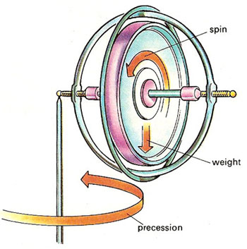
As for the topic of this post itself, we’re going to look at refraction again: light gets dispersed as it travels from one medium to another, as illustrated below.

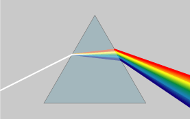
Dispersion literally means “distribution over a wide area”, and so that’s what happens as the light travels through the prism: the various frequencies (i.e. the various colors that make up natural ‘white’ light) are being separated out over slightly different angles. In physics jargon, we say that the index of refraction depends on the frequency of the wave – but so we could also say that the breaking angle depends on the color. But that sounds less scientific, of course. In any case, it’s good to get the terminology right. Generally speaking, the term refraction (as opposed to dispersion) is used to refer to the bending (or ‘breaking’) of light of a specific frequency only, i.e. monochromatic light, as shown in the photograph below. […] OK. We’re all set now.

$Refraction_photo$

It is interesting to note that the photograph above shows how the monochromatic light is actually being obtained: if you look carefully, you’ll see two secondary beams on the left-hand side (with an intensity that is much less than the central beam – barely visible in fact). That suggests that the original light source was sent through a diffraction grating designed to filter only one frequency out of the original light beam. That beam is then sent through a bloc of transparent material (plastic in this case) and comes out again, but displaced parallel to itself. So the block of plastics ‘offsets’ the beam. So how do we explain that in classical physics?

The index of refraction and the dispersion equation

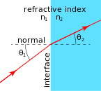
As I mentioned in my previous post, the Greeks had already found out, experimentally, what the index of refraction was. To be more precise, they had measured the θ₁ and θ₂ – depicted below – for light going from air to water. For example, if the angle in air (θ₁) is 20°, then the angle in the water (θ₂) will be 15°. It the angle in air is 70°, then the angle in the water will be 45°.

$Refraction_at_interface$

Of course, it should be noted that a lot of the light will also be reflected from the water surface (yes, imagine the romance of the image of the moon reflected on the surface of glacial lake while you’re feeling damn cold) – but so that’s a phenomenon which is better explained by introducing probability amplitudes, and looking at light as a bundle of photons, which we will not do here. I did that in previous posts, and so here, we will just acknowledge that there is a reflected beam but not say anything about it.

In any case, we should go step by step, and I am not doing that right now. Let’s first define the index of refraction. It is a number n which relates the angles above through the following relationship, which is referred to as Snell’s Law:

sinθ₁ = n sinθ₂

Using the numbers given above, we get: sin(20°) = n sin(15°), and sin(70°) = n sin(45°), so n must be equal to n = sin(20°)/sin(15°) = sin(70°)/sin(45°) ≈ 1.33. Just for the record, Willibrord Snell was a medieval Dutch astronomer but, according to Wikipedia, some smart Persian, Ibn Sahl, had already jotted this down in a treatise – “On Burning Mirrors and Lenses” – while he was serving the Abbasid court of Baghdad, back in 984, i.e. more than a thousand years ago! What to say? It was obviously a time when the Sunni-Shia divide did not matter, and Arabs and ‘Persians’ were leading civilization. I guess I should just salute the Islamic Golden Age here, regret the time lost during Europe’s Dark Ages and, most importantly, regret where Baghdad is right now ! And, as for the ‘burning’ adjective, it just refers to the fact that large convex lenses can concentrate the sun’s rays to a very small area indeed, thereby causing ignition. [It seems that story about Archimedes burning Roman ships with a ‘death ray’ using mirrors – in all likelihood: something that did not happen – fascinated them as well.]

But let’s get back at it. Where were we? Oh – yes – the refraction index. It’s (usually) a positive number written as n = 1 + some other number which may be positive or negative, and which depends on the properties of the material. To be more specific, it depends on the resonant frequencies of the atoms (or, to be precise, I should say: the resonant frequencies of the electrons bound by the atom, because it’s the charges that generate the radiation). Plus a whole bunch of natural constants that we have encountered already, most of which are related to electrons. Let me jot down the formula – and please don’t be scared away now (you can stop a bit later, but not now 🙂 please):

N is just the number of charges (electrons) per unit volume of the material (e.g. the water, or that block of plastic), and q_e and m are just the charge and mass of the electron. And then you have that electric constant once again, ε₀, and… Well, that’s it ! That’s not too terrible, is it? So the only variables on the right-hand side are ω₀ and ω, so that’s (i) the resonant frequency of the material (or the atoms – well, the electrons bound to the nucleus, to be precise, but then you know what I mean and so I hope you’ll allow me to use somewhat less precise language from time to time) and (ii) the frequency of the incoming light.

The equation above is referred to as the dispersion relation. It’s easy to see why: it relates the frequency of the incoming light to the index of refraction which, in turn, determinates that angle θ. So the formula does indeed determine how light gets dispersed, as a function of the frequencies in it, by some medium indeed (glass, air, water,…).

So the objective of this post is to show how we can derive that dispersion relation using classical physics only. As usual, I’ll follow Feynman – arguably the best physics teacher ever. 🙂 Let me warn you though: it is not a simple thing to do. However, as mentioned above, it goes to the heart of the “classical world view” in physics and so I do think it’s worth the trouble. Before we get going, however, let’s look at the properties of that formula above, and relate it some experimental facts, in order to make sure we more or less understand what it is that we are trying to understand. 🙂

First, we should note that the index of refraction has nothing to do with transparency. In fact, throughout this post, we’ll assume that we’re looking at very transparent materials only, i.e. materials that do not absorb the electromagnetic radiation that tries to go through them, or only absorb it a tiny little bit. In reality, we will have, of course, some – or, in the case of opaque (i.e. non-transparent) materials, a lot – of absorption going on, but so we will deal with that later. So, let me repeat: the index of refraction has nothing to do with transparency. A material can have a (very) high index of refraction but be fully transparent. In fact, diamond is a case in point: it has one of the highest indexes of refraction (2.42) of any material that’s naturally available, but it’s – obviously – perfectly transparent. [In case you’re interested in jewellery, the refraction index of its most popular substitute, cubic zirconia, comes very close (2.15-2.18) and, moreover, zirconia actually works better as a prism, so its disperses light better than diamond, which is why it reflects more colors. Hence, real diamond actually sparkles less than zirconia! So don’t be fooled! :-)]

Second, it’s obvious that the index of refraction depends on two variables indeed: the natural, or resonant frequency, ω₀, and the frequency ω, which is the frequency of the incoming light. For most of the ordinary gases, including those that make up air (i.e. nitrogen (78%) and oxygen (21%), plus some vapor (averaging 1%) and the so-called noble gas argon (0.93%) – noble because, just like helium and neon, it’s colorless, odorless and doesn’t react easily), the natural frequencies of the electron oscillators are close to the frequency of ultraviolet light. [The greenhouse gases are a different story – which is why we’re in trouble on this planet. Anyway…] So that’s why air absorbs most of the UV, especially the cancer-causing ultraviolet-C light (UVC), which is formally classified as a carcinogen by the World Health Organization. The wavelength of UVC light is 100 to 300 nanometer – as opposed to visible light, which has a wavelength ranging from 400 to 700 nm – and, hence, the frequency of UV light is in the 1000 to 3000 Teraherz range (1 THz = 10¹² oscillations per second) – as opposed to visible light, which has a frequency in the range of 400 to 800 THz. So, because we’re squaring those frequencies in the formula, ω² can then be disregarded in comparison with ω₀²: for example, 1500² = 2,250,000 and that’s not very different from 1500² – 500² = 2,000,000. Hence, if we leave the ω² out, we are still dividing by a very large number. That’s why n is very close to one for visible light entering the atmosphere from space (i.e. the vacuum). Its value is, in fact, around 1.000292 for incoming light with a wavelength of 589.3 nm (the odd value is the mean of so-called sodium D light, a pretty common yellow-orange light (street lights!), so that’s why it’s used as a reference value – however, don’t worry about it).

That being said, while the n of air is close to one for all visible light, the index is still slightly higher for blue light as compared to red light, and that’s why the sky is blue, except in the morning and evening, when it’s reddish. Indeed, the illustration below is a bit silly, but it gives you the idea. [I took this from http://mathdept.ucr.edu/ so I’ll refer you to that for the full narrative on that. :-)]

Where are we in this story? Oh… Yes. Two frequencies. So we should also note that – because we have two frequency variables – it also makes sense to talk about, for instance, the index of refraction of graphite (i.e. carbon in its most natural occurrence, like in coal) for x-rays. Indeed, coal is definitely not transparent to visible light (that has to do with the absorption phenomenon, which we’ll discuss later) but it is very ‘transparent’ to x-rays. Hence, we can talk about how graphite bends x-rays, for example. In fact, the frequency of x-rays is much higher than the natural frequency of the carbon atoms and, hence, in this case we can neglect the w₀² factor, so we get a denominator that is negative (because only the -w² remains relevant), so we get a refraction index that is (a bit) smaller than 1. [Of course, our body is transparent to x-rays too – to a large extent – but in different degrees, and that’s why we can take x-ray photographs of, for example, a broken rib or leg.]

OK. […] So that’s just to note that we can have a refraction index that is smaller than one and that’s not ‘anomalous’ – even if that’s a historical term that has survived.

Finally, last but not least as they say, you may have heard that scientists and engineers have managed to construct so-called negative index metamaterials. That matter is (much) more complicated than you might think, however, and so I’ll refer you to the Web if you want to find out more about that.

Light going through a glass plate: the classical idea

OK. We’re now ready to crack the nut. We’ll closely follow my ‘Great Teacher’ Feynman (Lectures, Vol. I-31) as he derives that formula above. Let me warn you again: the narrative below is quite complicated, but really worth the trouble – I think. The key to it all is the illustration below. The idea is that we have some electromagnetic radiation emanating from a far-away source hitting a glass plate – or whatever other transparent material. [Of course, nothing is to scale here: it’s just to make sure you get the theoretical set-up.]

So, as I explained in my previous post, the source creates an oscillating electromagnetic field which will shake the electrons up and down in the glass plate, and then these shaking electrons will generate their own waves. So we look at the glass as an assembly of little “optical-frequency radio stations” indeed, that are all driven with a given phase. It creates two new waves: one reflecting back, and one modifying the original field.

Let’s be more precise. What do we have here? First, we have the field that’s generated by the source, which is denoted by E_s above. Then we have the “reflected” wave (or field – not much difference in practice), so that’s E_b. As mentioned above, this is the classical theory, not the quantum-electrodynamical one, so we won’t say anything about this reflection really: just note that the classical theory acknowledges that some of the light is effectively being reflected.

OK. Now we go to the other side of the glass. What do we expect to see there? If we would not have the glass plate in-between, we’d have the same E_s field obviously, but so we don’t: there is a glass plate. 🙂 Hence, the “transmitted” wave, or the field that’s arriving at point P let’s say, will be different than E_s. Feynman writes it as E_s + E_a.

Hmm… OK. So what can we say about that? Not easy…

The index of refraction and the apparent speed of light in a medium

Snell’s Law – or Ibn Sahl’s Law – was re-formulated, by a 17^th century French lawyer with an interesting in math and physics, Pierre de Fermat, as the Principle of Least Time. It is a way of looking at things really – but it’s very confusing actually. Fermat assumed that light traveling through a medium (water or glass, for instance) would travel slower, by a certain factor n, which – indeed – turns out to be the index of refraction. But let’s not run before we can walk. The Principle is illustrated below. If light has to travel from point S (the source) to point D (the detector), then the fastest way is not the straight line from S to D, but the broken S-L-D line. Now, I won’t go into the geometry of this but, with a bit of trial and error, you can verify for yourself that it turns out that the factor n will indeed be the same factor n as the one which was ‘discovered’ by Ibn Sahl: sinθ₁ = n sinθ₂.

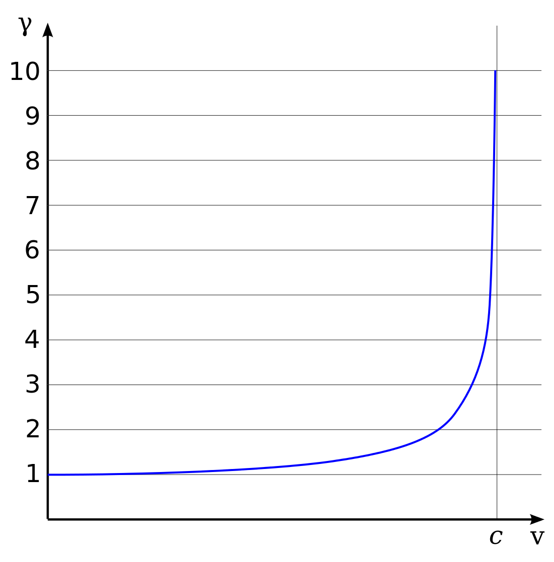
What we have then, is that the apparent speed of the wave in the glass plate that we’re considering here will be equal to v = c/n. The apparent speed? So does that mean it is not the real speed? Hmm… That’s actually the crux of the matter. The answer is: yes and no. What? An ambiguous answer in physics? Yes. It’s ambiguous indeed. What’s the speed of a wave? We mentioned above that n could be smaller than one. Hence, in that case, we’d have a wave traveling faster than the speed of light. How can we make sense of that?

We can make sense of that by noting that the wave crests or nodes may be traveling faster than c, but that the wave itself – as a signal – cannot travel faster than light. It’s related to what we said about the difference between the group and phase velocity of a wave. The phase velocity – i.e. the nodes, which are mathematical points only – can travel faster than light, but the signal as such, i.e. the wave envelope in the illustration below, cannot.

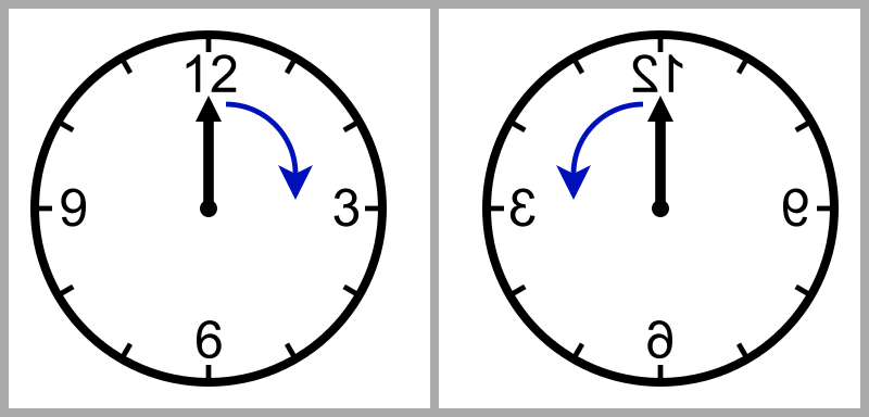
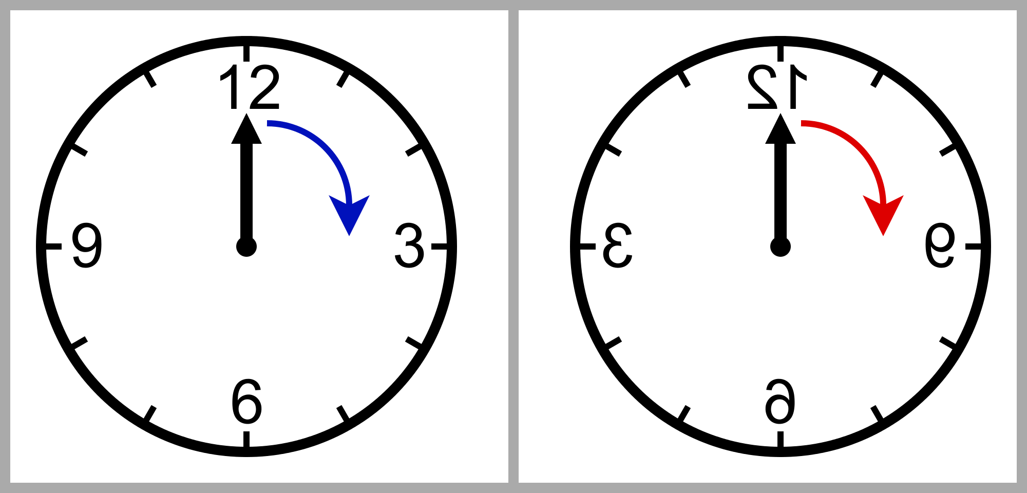
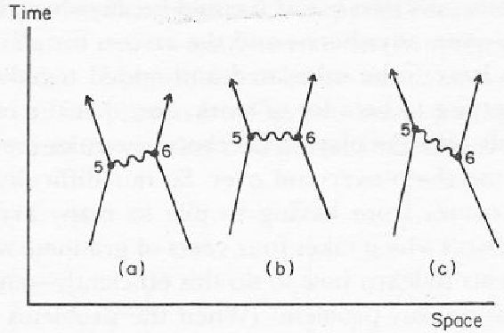
What is happening really is the following. A wave will hit one of these electron oscillators and start a so-called transient, i.e. a temporary response preceding the ‘steady state’ solution (which is not steady but dynamic – confusing language once again – so sorry!). So the transient settles down after a while and then we have an equilibrium (or steady state) oscillation which is likely to be out of phase with the driving field. That’s because there is damping: the electron oscillators resist before they go along with the driving force (and they continue to put up resistance, so the oscillation will die out when the driving force stops!). The illustration below shows how it works for the various cases:

In case (b), the phase of the transmitted wave will appear to be delayed, which results in the wave appearing to travel slower, because the distance between the wave crests, i.e. the wavelength λ, is being shortened. In case (c), it’s the other way around: the phase appears to be advanced, which translated into a bigger distance between wave crests, or a lengthening of the wavelength, which translates into an apparent higher speed of the transmitted wave.

So here we just have a mathematical relationship between the (apparent) speed of a wave and its wavelength. The wavelength is the (apparent) speed of the wave (that’s the speed with which the nodes of the wave travel through space, or the phase velocity) divided by the frequency: λ = v_p/f. However, from the illustration above, it is obvious that the signal, i.e. the start of the wave, is not earlier – or later – for either wave (b) and (c). In fact, the start of the wave, in time, is exactly the same for all three cases. Hence, the electromagnetic signal travels at the same speed c, always.

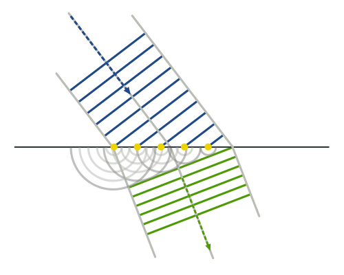
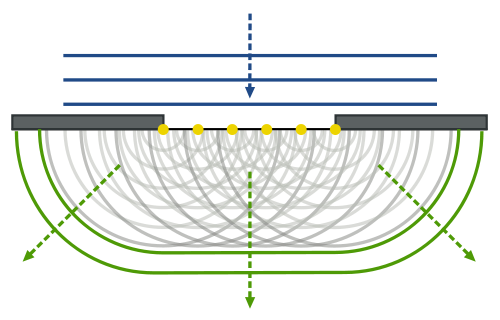
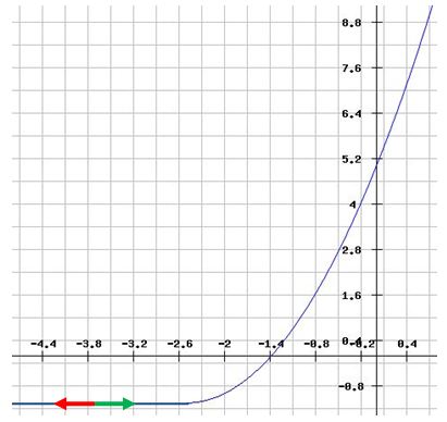
While this may seem obvious, it’s quite confusing, and therefore I’ll insert one more illustration below. What happens when the various wave fronts of the traveling field hit the glass plate (coming from the top-left hand corner), let’s say at time t = t₀, as shown below, is that the wave crests will have the same spacing along the surface. That’s obvious because we have a regular wave with a fixed frequency and, hence, a fixed wavelength λ₀, here. Now, these wave crests must also travel together as the wave continues its journey through the glass, which is what is shown by the red and green arrows below: they indicate where the wave crest is after one and two periods (T and 2T) respectively.

To understand what’s going on, you should note that the frequency f of the wave that is going through the glass sheet and, hence, its period T, has not changed. Indeed, the driven oscillation, which was illustrated for the two possible cases above (n > 1 and n < 1), after the transient has settled down, has the same frequency (f) as the driving source. It must. Always. That being said, the driven oscillation does have that phase delay (remember: we’re in the (b) case here, but we can make a similar analysis for the (c) case). In practice, that means that the (shortest) distance between the crests of the wave fronts at time t = t₀ and the crests at time t₀ + T will be smaller. Now, the (shortest) distance between the crests of a wave is, obviously, the wavelength divided by the frequency: λ = v_p/f, with v_p the speed of propagation, i.e. the phase velocity, of the wave, and f = 1/T. [The frequency f is the reciprocal of the period T – always. When studying physics, I found out it’s useful to keep track of a few relationships that hold always, and so this is one of them. :-)]

Now, the frequency is the same, but so the wavelength is shortened as the wave travels through the various layers of electron oscillators, each causing a delay of phase – and, hence, a shortening of the wavelength, as shown above. But, if f is the same, and the wavelength is shorter, then v_p cannot be equal to the speed of the incoming light, so v_p ≠ c. The apparent speed of the wave traveling through the glass, and the associated shortening of the wavelength, can be calculated using Snell’s Law. Indeed, knowing that n ≈ 1.33, we can calculate the apparent speed of light through the glass as v = c/n ≈ 0.75c and, therefore, we can calculate the wavelength of the wave in the glass l as λ = 0.75λ₀.

OK. I’ve been way too lengthy here. Let’s sum it all up:

The field in the glass sheet must have the shape that’s depicted above: there is no other way. So that means the direction of ‘propagation’ has been changed. As mentioned above, however, the direction of propagation is a ‘mathematical’ property of the field: it’s not the speed of the ‘signal’.
Because the direction of propagation is normal to the wave front, it implies that the bending of light rays comes about because the effective speed of the waves is different in the various materials or, to be even more precise, because the electron oscillators cause a delay of phase.
While the speed and direction of propagation of the wave, i.e. the phase velocity, accurately describes the behavior of the field, it is not the speed with which the signal is traveling (see above). That is why it can be larger or smaller than c, and so it should not raise any eyebrow. For x-rays in particular, we have a refractive index smaller than one. [It’s only slightly less than one, though, and, hence, x-ray images still have a very good resolution. So don’t worry about your doctor getting a bad image of your broken leg. 🙂 In case you want to know more about this: just Google x-ray optics, and you’ll find loads of information. :-)]

Calculating the field

Are you still there? Probably not. If you are, I am afraid you won’t be there ten or twenty minutes from now. Indeed, you ain’t done nothing yet. All of the above was just setting the stage: we’re now ready for the pièce de résistance, as they say in French. We’re back at that illustration of the glass plate and the various fields in front and behind the plate. So we have electron oscillators in the glass plate. Indeed, as Feynman notes: “As far as problems involving light are concerned, the electrons behave as though they were held by springs. So we shall suppose that the electrons have a linear restoring force which, together with their mass m, makes them behave like little oscillators, with a resonant frequency ω₀.”

So here we go:

1. From everything I wrote about oscillators in previous posts, you should remember that the equation for this motion can be written as m[d²x/dt²+ ω₀²) = F. That’s just Newton’s Law. Now, the driving force F comes from the electric field and will be equal to F = q_eE_s.

Now, we assume that we can chose the origin of time (i.e. the moment from which we start counting) such that the field E_s = E₀cos(ωt). To make calculations easier, we look at this as the real part of a complex function E_s = E₀eⁱ^ωt. So we get:

m[d²x/dt²+ ω₀²] = q_eE₀eⁱ^ωt

We’ve solved this before: its solution is x = x₀eⁱ^ωt. We can just substitute this in the equation above to find x₀ (just substitute and take the first- and then second-order derivative of x indeed): x₀ = q_eE₀/m(ω₀²-ω²). That, then, gives us the first piece in this lengthy derivation:

x = q_eE₀eⁱ^ωt/m(ω₀²-ω²)

Just to make sure you understand what we’re doing: this piece gives us the motion of the electrons in the plate. That’s all.

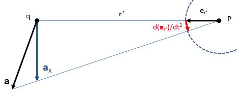
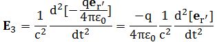
2. Now, we need an equation for the field produced by a plane of oscillating charges, because that’s what we’ve got here: a plate or a plane of oscillating charges. That’s a complicated derivation in its own, which I won’t do there. I’ll just refer to another chapter of Feynman’s Lectures (Vol. I-30-7) and give you the solution for it (if I wouldn’t do that, this post would be even longer than it already is):

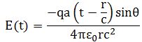
This formula introduces just one new variable, η, which is the number of charges per unit area of the plate (as opposed to N, which was the number of charges per unit volume in the plate), so that’s quite straightforward. Less straightforward is the formula itself: this formula says that the magnitude of the field is proportional to the velocity of the charges at time t – z/c, with z the shortest distance from P to the plane of charges. That’s a bit odd, actually, but so that’s the way it comes out: “a rather simple formula”, as Feynman puts it.

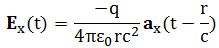
In any case, let’s use it. Differentiating x to get the velocity of the charges, and plugging it into the formula above yields:

Note that this is only E_a, the additional field generated by the oscillating charges in the glass plate. To get the total electric field at P, we still have to add E_s, i.e. the field generated by the source itself. This may seem odd, because you may think that the glass plate sort of ‘shields’ the original field but, no, as Feynman puts it: “The total electric field in any physical circumstance is the sum of the fields from all the charges in the universe.”

3. As mentioned above, z is the distance from P to the plate. Let’s look at the set-up here once again. The transmitted wave, or E_{after the plate} as we shall note it, consists of two components: E_s and E_a. E_s here will be equal to (the real part of) E_s = E₀eⁱ^ω(t^-z/c). Why t – z/c instead of just t? Well… We’re looking at E_s here as measured in P, not at E_s at the glass plate itself.

Now, we know that the wave ‘travels slower’ through the glass plate (in the sense that its phase velocity is less, as should be clear from the rather lengthy explanation on phase delay above, or – if n would be greater than one – a phase advance). So if the glass plate is of thickness Δz, and the phase velocity is is v = c/n, then the time it will take to travel through the glass plate will be Δz/(c/n) instead of Δz/c (speed is distance divided by time and, hence, time = distance divided by speed). So the additional time that is needed is Δt = Δz/(c/n) – Δz/c = nΔz/c – Δz/c = (n-1)Δz/c. That, then, implies that E_{after the plate} is equal to a rather monstrously looking expression:

E_{after plate} = E₀eⁱ^ω^[t^–⁽ⁿ^–^1)Δ^z/c^–^z/c) = e^–ⁱ^ω⁽ⁿ^–^1)Δ^z/c)E₀eⁱ^ω^(t^–^z/c)

We get this by just substituting t for t – Δt.

So what? Well… We have a product of two complex numbers here and so we know that this involves adding angles – or substracting angles in this case, rather, because we’ve got a minus sign in the exponent of the first factor. So, all that we are saying here is that the insertion of the glass plate retards the phase of the field with an amount equal to w(n-1)Δz/c. What about that sum E_{after the plate} = E_s + E_a that we were supposed to get?

Well… We’ll use the formula for a first-order (linear) approximation of an exponential once again: e^x ≈ 1 + x. Yes. We can do that because Δz is assumed to be very small, infinitesimally small in fact. [If it is not, then we’ll just have to assume that the plate consists of a lot of very thin plates.] So we can write that e^–i^ω(n^-1)^Δz/c) = 1 – iω(n-1)Δz/c, and then we, finally, get that sum we wanted:

E_{after plate} = E₀eⁱ^ω^[t^–^z/c)− iω(n-1)Δz·E₀eⁱ^ω^(t^–^z/c)/c

The first term is the original E_s field, and the second term is the E_a field. Geometrically, they can be represented as follows:

Why is E_a perpendicular to E_s? Well… Look at the –i = 1/i factor. Multiplication with –i amounts to a clockwise rotation by 90°, and then just note that the magnitude of the vector must be small because of the ω(n-1)Δz/c factor.

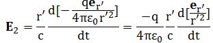
4. By now, you’ve either stopped reading (most probably) or, else, you wonder what I am getting at. Well… We have two formulas for E_a now:

and E_a = – iω(n-1)Δz·E₀eⁱ^ω(t^{– z/c)}/c

Equating both yields:

But η, the number of charges per unit area, must be equal to NΔz, with N the number of charges per unit volume. Substituting and then cancelling the Δz finally gives us the formula we wanted, and that’s the classical dispersion relation whose properties we explored above:

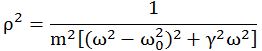
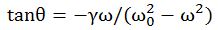
Absorption and the absorption index

The model we used to explain the index of refraction had electron oscillators at its center. In the analysis we did, we did not introduce any damping factor. That’s obviously not correct: it means that a glass plate, once it had illuminated, would continue to emit radiation, because the electrons would oscillate forever. When introducing damping, the denominator in our dispersion relation becomes m(ω₀² – ω² + iγω), instead of m(ω₀² – ω²). We derived this in our posts on oscillators. What it means is that the oscillator continues to oscillate with the same frequency as the driving force (i.e. not its natural frequency) – so that doesn’t change – but that there is an envelope curve, ensuring the oscillation dies out when the driving force is no longer being applied. The γ factor is the damping factor and, hence, determines how fast the damping happens.

We can see what it means by writing the complex index of refraction as n = n’ – in’’, with n’ and n’’ real numbers, describing the real and imaginary part of n respectively. Putting that complex n in the equation for the electric field behind the plate yields:

E_{after plate} = e^–^ω^n’’^Δ^z/ce^–ⁱ^ω^(n’^–^1)Δ^z/cE₀eⁱ^ω(t^–^z/c)

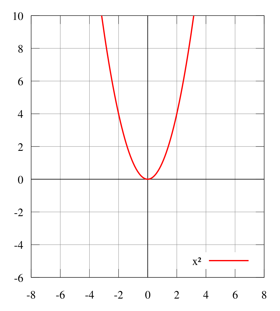
This is the same formula that we had derived already, but so we have an extra exponential factor: e^–^ωn’’^Δz/c. It’s an exponential factor with a real exponent, because there were two i‘s that cancelled. The e^-x function has a familiar shape (see below): e^-x is 1 for x = 0, and between 0 and 1 for any value in-between. That value will depend on the thickness of the glass sheet. Hence, it is obvious that the glass sheet weakens the wave as it travels through it. Hence, the wave must also come out with less energy (the energy being proportional to the square of the amplitude). That’s no surprise: the damping we put in for the electron oscillators is a friction force and, hence, must cause a loss of energy.

Note that it is the n’’ term – i.e. the imaginary part of the refractive index n – that determines the degree of absorption (or attenuation, if you want). Hence, n’’ is usually referred to as the “absorption index”.

The complete dispersion relation

We need to add one more thing in order to get a fully complete dispersion relation. It’s the last thing: then we have a formula which can really be used to describe real-life phenomena. The one thing we need to add is that atoms have several resonant frequencies – even an atom with only one electron, like hydrogen ! In addition, we’ll usually want to take into account the fact that a ‘material’ actually consists of various chemical substances, so that’s another reason to consider more than one resonant frequency. The formula is easily derived from our first formula (see the previous post), when we assumed there was only one resonant frequency. Indeed, when we have N_k electrons per unit of volume, whose natural frequency is ω_k and whose damping factor is γ_k, then we can just add the contributions of all oscillators and write:

The index described by this formula yields the following curve:

So we have a curve with a positive slope, and a value n > 1, for most frequencies, except for a very small range of ω’s for which the slope is negative, and for which the index of refraction has a value n < 1. As Feynman notes, these ω’s– and the negative slope – is sometimes referred to as ‘anomalous’ dispersion but, in fact, there’s nothing ‘abnormal’ about it.

The interesting thing is the iγ_kω term in the denominator, i.e. the imaginary component of the index, and how that compares with the (real) “resonance term” ω_k²– ω². If the resonance term becomes very small compared to iγ_kω, then the index will become almost completely imaginary, which means that the absorption effect becomes dominant. We can see that effect in the spectrum of light that we receive from the sun: there are ‘dark lines’, i.e. frequencies that have been strongly absorbed at the resonant frequencies of the atoms in the Sun and its ‘atmosphere’, and that allows us to actually tell what the Sun’s ‘atmosphere’ (or that of other stars) actually consists of.

So… There we are. I am aware of the fact that this has been the longest post of all I’ve written. I apologize. But so it’s quite complete now. The only piece that’s missing is something on energy and, perhaps, some more detail on these electron oscillators. But I don’t think that’s so essential. It’s time to move on to another topic, I think.

Some content on this page was disabled on June 17, 2020 as a result of a DMCA takedown notice from Michael A. Gottlieb, Rudolf Pfeiffer, and The California Institute of Technology. You can learn more about the DMCA here:

https://wordpress.com/support/copyright-and-the-dmca/
Some content on this page was disabled on June 17, 2020 as a result of a DMCA takedown notice from Michael A. Gottlieb, Rudolf Pfeiffer, and The California Institute of Technology. You can learn more about the DMCA here:

https://wordpress.com/support/copyright-and-the-dmca/
Some content on this page was disabled on June 17, 2020 as a result of a DMCA takedown notice from Michael A. Gottlieb, Rudolf Pfeiffer, and The California Institute of Technology. You can learn more about the DMCA here:

https://wordpress.com/support/copyright-and-the-dmca/
Some content on this page was disabled on June 17, 2020 as a result of a DMCA takedown notice from Michael A. Gottlieb, Rudolf Pfeiffer, and The California Institute of Technology. You can learn more about the DMCA here:

https://wordpress.com/support/copyright-and-the-dmca/

Euler’s spiral

Pre-scriptum (dated 26 June 2020): Most of the relevant illustrations in this post were removed as a result of an attack by the dark force. Too bad, because I liked this post. In any case, despite the removal of the illustrations, you should be able to reconstruct the main story line.

Original post:

When talking diffraction, one of the more amusing curves is the curve showing the intensity of light near the edge of a shadow. It is shown below.

Light becomes more intense as we move away from the edge, then it overshoots (so it is brighter than further away), then the intensity wobbles and oscillates, to finally ‘settle’ at the intensity of the light elsewhere.

How do we get a curve like that? We get it through another amusing curve: the Cornu spiral (which was re-named as the Euler spiral for some reason I don’t understand), which we’ve encountered also when adding probability amplitudes. Let me first depict the ‘real’ situation below: we have an opaque object AB, so no light goes through AB itself. However, the light that goes past it, casts a shadow on a screen, which is denoted as QPR here. And so the curve above shows the intensity of the light near the edge of that shadow.

The first weird thing to note is what I said about diffraction of light through a slit (or a hole – in somewhat less respectful language) in my previous post: the diffraction patterns can be explained if we assume that there are sources distributed, with uniform density, across the open holes. This is a deep mystery, which I’ll attempt to explain later. As for now, I can only state what Feynman has to say about it: “Of course, actually there are no sources at the holes. In fact, that is the only place that there are certainly no sources. Nevertheless, we get the correct diffraction pattern by considering the holes to be the only places where there are sources.”

So we do the same here. We assume that we have a series of closely spaced ‘antennas’, or sources, starting from B, up to D, E, C and all the way up to infinity, and so we need to add the contributions – or the waves – from these sources to calculate the intensity at all of the points on the screen. Let’s start with the (random) point P. P defines the inflection point D: we’ll say the phase there is zero (because we can, of course, choose our point in time so as to make it zero). So we’ll associate the contribution from D with a tiny vector (an infinitesimal vector) with angle zero. That is shown below: it’s the ‘flat’ (horizontal) vector pointing straight east at the very center of this so-called Cornu spiral.

Now, in the neighborhood of D, i.e. just below or above point D, the phase difference will be very small, because the distance from those points near D to P will not differ much from the distance between D and P (i.e. the distance DP). However, as h increases, the phase difference will become larger and larger, it will not increase linearly with h but, because of the geometry involved, the path difference – and, hence, the phase difference (remember – from the previous post – that the phase difference was the product of the wave number and the difference in distance) will increase proportionally with the square of h. In fact, using similar triangles once again, we can easily show that this path difference EF can be approximated by EF ≈ h²/s. However, don’t lose sleep if you wouldn’t manage to figure that out. 🙂

The point to note is that, when you look at that spiral above, the angle of each vector that we’re adding, increases more and more, so that’s why we get a spiral, and not a polygon in a circle, such as the one we encountered in our previous post: the phase differences there were linearly proportional and, hence, each vector added a constant angle to the previous one. Likewise, if we go down from D, to the edge B, the angles will decrease. Of course, if we’re adding contributions to get the amplitude or intensity for point P, we will not get any contributions from points below B. The last (or, I should say, the first) contribution that we get is denoted by the vector B_P on that spiral curve, so if we want to get the total contribution, then we have to start adding vectors from there. [Don’t worry: you’ll understand why the other vectors, ‘down south’, are there in a few minutes.]

So we start from B_P and go all the way… Well… You see that, once, we’re ‘up north’, in the center of the upper-most spiral, we’re not adding much anymore, because the additional vectors are just sharply changing direction and going round and round and round. In short, most of the contribution to the amplitude of the resultant vector B_P∞ is given by points near D. Now, we have chosen point P randomly, and you can easily see from that Cornu spiral that the amplitude, or the intensity rather (which is the square of the amplitude) of that vector B_P∞, increases initially, to reach some maximum, depending upon where P is located above B, but then it falls and oscillates indeed, producing the curve with which we started this post.

OK. […] So what else do we have here? Well… That Cornu spiral also shows how we should add arrows to get the intensity at point Q. We’d be adding arrows in the upper-most spiral only and, hence, we would not get much of a total contribution as a result. That’s what marked by vector B_Q. On the other hand, if we’d be adding contributions to calculate the intensity at a point much higher than P, i.e. R, then we’d be using pretty much all of the arrows, down from the spiral ‘south’ all the way up to the spiral ‘north’. So that’s B_R obviously and, as you can see, most of the contribution comes, once again, from points near D, so that’s the points near the edge. [So now you know why we have an infinite number of arrows in both directions: we need to be able to calculate the intensity from any point on the screen really, below or above P.]

OK. What else? Well… Nothing. This is it really − for the moment that is. Just note that we’re not adding probability amplitudes here (unlike what we did a couple of months ago). We’re adding vectors representing something real here: electric field vectors. [As for how ‘real’ they are: I’ll entertain you about that later. :-)]

This was rather short, isn’t it? I hope you liked it because… Well… What will follow is actually much more boring, because it involves a lot more formulas. However, these formulas will help us get where we want to get, and that is to understand – somehow, if only from a classical perspective – why that empty space acts like an array of electromagnetic radiation sources.

Indeed, when everything is said and done, that’s the deep mystery of light really. Really really deep.

Some content on this page was disabled on June 17, 2020 as a result of a DMCA takedown notice from Michael A. Gottlieb, Rudolf Pfeiffer, and The California Institute of Technology. You can learn more about the DMCA here:

https://wordpress.com/support/copyright-and-the-dmca/
Some content on this page was disabled on June 17, 2020 as a result of a DMCA takedown notice from Michael A. Gottlieb, Rudolf Pfeiffer, and The California Institute of Technology. You can learn more about the DMCA here:

https://wordpress.com/support/copyright-and-the-dmca/
Some content on this page was disabled on June 17, 2020 as a result of a DMCA takedown notice from Michael A. Gottlieb, Rudolf Pfeiffer, and The California Institute of Technology. You can learn more about the DMCA here:

https://wordpress.com/support/copyright-and-the-dmca/

Diffraction gratings

Pre-scriptum (dated 26 June 2020): Some of the relevant illustrations in this post were removed as a result of an attack by the dark force. Too bad, because I liked this post. In any case, despite the removal of the illustrations, I think you will still be able to reconstruct the main story line.

Original post:

Diffraction gratings are fascinating. The iridescent reflections from the grooves of a compact disc (CD), or from oil films, soap bubbles: it is all the same principle (or closely related – to be precise). In my April, 2014 posts, I introduced Feynman’s ‘arrows’ to explain it. Those posts talked about probability amplitudes, light as a bundle of photons, quantum electrodynamics. They were not wrong. In fact, the quantum-electrodynamical explanation is actually the only one that’s 100% correct (as far as we ‘know’, of course). But it is also more complicated than the classical explanation, which just explains light as waves.

To understand the classical explanation, one first needs to understand how electromagnetic waves interfere. That’s easy, you’ll say. It’s all about adding waves, isn’t it? And we have done that before, haven’t we? Yes. We’ve done it for sinusoidal waves. We also noted that, from a math point of view, the easiest way to go about it was to use vectors or complex numbers, and equate the real parts of the complex numbers with the actual physical quantities, i.e. the electric field in this case.

You’re right. Let’s continue to work with sinusoidal waves, but instead of having just two waves, we’ll consider a whole array of sources, because that’s what we’ll need to analyze when analyzing a diffraction grating.

First the simple case: two sources

Let’s first re-analyze the simple situation: two sources – or two dipole radiators as I called them in my previous post. The illustration below gives a top view of two such oscillators. They are separated, in the north-south direction, by a distance d.

Is that realistic? It is for radio waves: the wavelength of a 1 megahertz radio wave is 300 m (remember: λ = c/f). So, yes, we can separate two sources by a distance in the same order of magnitude as the wavelength of the radiation, but, as Feynman writes: “We cannot make little optical-frequency radio stations and hook them up with infinitesimal wires and drive them all with a given phase.”

For light, it will work differently – and we’ll describe how, but not now. As for now, we should continue with our radio waves.

The illustration above assumes that the radiation from the two sources is sinusoidal and has the same (maximum) amplitude A, but that the two sources might be out of phase: we’ll denote the difference by α. Hence, we can represent the radiation emitted by the two sources by the real part of the complex numbers Aeⁱ^ωt and Aeⁱ⁽^{ωt + α}⁾ respectively. Now, we can move our detector around to measure the intensity of the radiation from these two antennas. If we place our detector at some point P, sufficiently far away from the sources, then the angle θ will result in another phase difference, due to the difference in distance from point P to the two oscillators. From simple geometry, we know that this difference will be equal to d·sinθ. The phase difference due to the distance difference will then be equal to the product of the wave number k (i.e. the rate of change of the phase (expressed in radians) with distance, i.e. per meter) and that distance d·sinθ. So the phase difference at arrival (i.e. at point P) would be

Φ₂ – Φ₁ = α + k· d·sinθ = α + (2π/λ)·d·sinθ

That’s pretty obvious, but let’s play a bit with this, in order to make we understand what’s going on. The illustration below gives two examples: α = 0 and α = π.

How do we get these numbers 0, 2 and 4, which indicate the intensity, i.e. the amount of energy that the field carries past per second, which is proportional to the square of the field, averaged in time? [If it would be (visible) light, instead of radio waves, the intensity would be the brightness of the light.]

Well… In the first case, we have α = 0 and d = λ/2 and, hence, at an angle of 30 degrees, we have d·sin(30°) = (λ/2)(1/2) = λ/4. Therefore, Φ₂ – Φ₁ = α + (2π/λ)·d·sinθ = 0 + (2π/λ)·(λ/4) = π/2. So what? Well… Let’s add the waves. We will have some combined wave with amplitude A_R and phase Φ_R:

Now, to calculate the length of this ‘vector’, i.e. the amplitude A_R, we take the product of this complex number and its complex conjugate, and that will give us the length squared, and then we multiply it all out and so on and so on. To make a long story short, we’ll find that

A_R² = A₁² + A₂² + 2A₁A₂cos(Φ₂ – Φ₁)

The last term in this sum is the interference effect, and so that’s equal to zero in the case we’ve been studying above (α = 0, d = λ/2 and θ = 30°), so we get twice the intensity of one oscillator only. The other cases can be worked out in the same way.

Now, you should not think that the pattern is always symmetric, or simple, as the two illustrations below make clear.

With more oscillators, the patterns become even more interesting. The illustration below shows part of the intensity pattern of a six-dipole antenna array:

Let’s look at that now indeed: arrays with n oscillators.

Arrays with n oscillators

If we have six oscillators, like in the illustration above, we have to add something like this:

R = A[cos(ωt) + cos(ωt + Φ) + cos(ωt + 2Φ) + … + cos(ωt + 5Φ)]

From what we wrote above, it is obvious that the phase difference Φ can have two causes: the oscillators may be driven differently in phase, or we may be looking at them at an angle so that there is a difference in time delay. Hence, we have the same formula as the one above:

Φ = α + (2π/λ)·d·sinθ

Now, we have an interesting geometrical approach to finding the net amplitude A_R. We can, once again, consider the various waves as vectors and add them, as shown below.

The length of all vectors is the same (A), and then we have the phase difference, i.e. the different angles: zero for A₁, Φ for A₁, 2Φ for A₂, etcetera. So as we’re adding these vectors, we’re going around and forming an equiangular polygon with n sides, with the vertices (corner points) lying on a circle with radius r. It requires just a bit of trigonometry to establish that the following equality must hold: A = 2rsin(Φ/2). So that fixes r. We also have that the large angle OQT equals nΦ and, hence, A_R = 2rsin(nΦ/2). We can now combine the results to find the following amplitude and intensity formula:

This formula is obvious for n = 1 and for n = 2: it gives us the results which were shown above already. But here we want to know how this thing behaves for large n. It is easy to see that the numerator above, i.e. sin²(nΦ/2), will always be larger than the denominator, sin²(Φ/2), and that both are – obviously – smaller or equal to 1. It can be demonstrated that this function of the angle Φ reaches its maximum value for Φ = 0. Indeed, taking the limit gives us I = I₀n². [We can intuitively see this because, if we express the angle in radians, we can substitute sin(Φ/2) and sin(nΦ/2) for Φ/2 and nΦ/2, and then we can eliminate the (Φ/2)² factor to get n².

It’s a bit more difficult to understand what happens next. If Φ becomes a bit larger, the ratio of the two sines begins to fall off (so it becomes smaller than n²). Note that the numerator, i.e. sin²(nΦ/2), will be equal to one if nΦ/2 = π/2, i.e. if Φ = π/n, and the ratio sin²(nΦ/2)/sin²(Φ/2) then becomes sin²(π/2)/sin²(π/2n) = 1/sin²(π/2n). Again, if we assume that n is (very) large, we can approximate and write that this ratio is more or less equal to 1/(π²/4n²) = 4n²/π². That means that the intensity there will be 4/ π² times the intensity of the beam at the maximum, i.e. 40.53% of it. That’s the point at nΦ/2π = 0.5 on the graph below.

The graph above has a re-scaled vertical as well as a re-scaled horizontal axis. Indeed, instead of I, the vertical axis shows I/n²I₀, so the maximum value is 1. And the horizontal axis does not show Φ but nΦ/2π, so if Φ = π/n, then nΦ/2π = 0.5 indeed. [Don’t worry about the dotted curve: that’s the solid-line curve multiplied by 10: it’s there to make sure you see what’s going on, as this ratio of those sines becomes very small very rapidly indeed.]

So, once we’re past that 40.53% point, we get at our first minimum, which is reached at nΦ/2π = 1 or Φ = 2π/n. The numerator sin²(nΦ/2) equals sin²(π) = 0 there indeed, so the whole ratio becomes zero. Then it goes up again, to our second maximum, which we get when our numerator comes close to one again, i.e. when sin²(nΦ/2) ≈ 1. That happens when nΦ/2 = 3π/2, or Φ = 3π/n. Again, when n is (very) large, Φ will be very small, and so we can substitute the denominator sin²(Φ/2) for Φ²/4. We then get a ratio equal to 1/(9π²/4), or an intensity equal to 4n²I₀/9π², i.e. only 4.5% of the intensity at the (first) maximum. So that’s tiny. [Well… All is relative, of course. :-)] We can go on and on like that but that’s not the point here: the point is that we have a very sharp central maximum with very weak subsidiary maxima on the sides.

But what about that big lobe at 30 degrees on that graph with the six-dipole antenna? Relax. We’re not done yet with this ‘quick’ analysis. Let’s look at the general case from yet another angle, so to say. 🙂

The general case

To focus our minds, we’ve depicted that array with n oscillators below. Once again, we note that the phase difference between two sources, one to the next, will depend on (1) the intrinsic phase difference between them, which we denote by α, and (2) the time delay because we’re observing the system in a given direction q from the normal, which effect we calculated as equal to (2π/λ)·d·sinθ. So the whole effect is Φ = α + (2π/λ)·d·sinθ = a + k·d·sinθ, with k the wave number.

To make things simple, let’s first assume that α = 0. We’re then in the case that we described above: we’ll have a sharp maximum at Φ = 0, so that means θ = 0. It’s easy to see why: all oscillators are in phase and so we have maximum positive (or constructive) interference.

Let’s now examine the first minimum. When looking back at that geometrical interpretation, with the polygon, all the arrows come back to the starting point: we’ve completed a full circle. Indeed, n times Φ gives nΦ = n·2π/n = 2π. So what’s going on here? Well… If we put that value in our formula Φ = α + (2π/λ)·d·sinθ, we get 2π/n = 0 + (2π/λ)·d·sinθ or, getting rid of the 2π factor, n·d·sinθ = λ.

Now, n·d is the total length of the array, i.e. L, and, from the illustration above, we see that n·d·sinλ = L·sinθ = Δ. So we have that n·d·sinθ = λ = Δ. Hence, Δ is equal to one wavelength.That means that the total phase difference between the first and the last oscillator is equal to 2π, and the contributions of all the oscillators in-between are uniformly distributed in phase between 0° and 360°. The net result is a vector A_R with amplitude A_R = 0 and, hence, the intensity is zero as well.

OK, you’ll say, you’re just repeating yourself here. What about the other lobe or lobes? Well… Let’s go back to that maximum. We had it at Φ = 0, but we will also have it at Φ = 2π, and at Φ = 4π, and at Φ = 6π etcetera, etcetera. We’ll have such sharp maximum – the maximum, in fact – at any Φ = m⋅2π, where m is any integer. Now, plugging that into the Φ = α + (2π/λ)·d·sinθ formula (again, assuming that α = 0), we get m⋅2π = (2π/λ)·d·sinθ or d·sinθ = mλ.

While that looks very similar to our n·d·sinθ = λ = Δ condition for the (first) minimum, we’re not looking at that Δ but at that δ angle measured from the individual sources, and so we have δ = Δ/n = mλ. What’s being said here, is that each successive source is out of phase by 360° and, because, being out of phase by 360° obviously means that you’re in phase once again, ensure that all sources are, once again, contributing in phase and produce a maximum that is just as good as the one we had for m = 0. Now, these maxima will also have a (first) minimum described by that other formula above, and so that’s how we get that pattern of lobes with weak ‘side lobes’.

Conditions

Now, the conditions presented above for maxima and minima obviously all depend on the distance d, i.e. the spacing of the array, and the wavelength λ. That brings us to an interesting point: if d is smaller than λ (so if the spacing is smaller than one wavelength), we have (d/λ)·sinθ = m < 1, so we only have one solution for m: m = 0. So we only have on beam in that case, the so-called zero-order beam centered at θ = 0. [Note that we also have a beam in the opposite direction.]

The point to note is that we can only have subsidiary great maxima if the spacing d of the array is greater than the wavelength λ. If we have such subsidiary great maxima, we’ll call them first-order, second-order etcetera beams, according to the value m.

Diffraction gratings

We are now, finally, ready to discuss diffraction gratings. A diffraction grating, in its simplest form, is a plane glass sheet with scratches on it: several hundred grooves, or several thousand even, to the millimeter. That is because the spacing has to be of the same order of magnitude of the wavelength of light, so that’s 400 to 700 nanometer (nm) indeed – with the 400-500 nm range corresponding to violet-blue light, and the (longer) 700+ nm range corresponding to red light. Remember, a nanometer is a billionth of a meter (1´10^-9 m), so even one thousandth of a millimeter is 1000 nanometer, i.e. longer than the wavelength of red light. Of course, from what we wrote above, it is obvious that the spacing d must be wider than the wavelength of interest to cause second- and third-order beams and, therefore, diffraction but, still, the order of magnitude must be the same to produce anything of interest. Isn’t it amazing that scientists were able to produce such diffraction experiments around the turn of the 18^th century already? One of the earliest apparatuses, made in 1785, by the first director of the United States Mint, used hair strung between two finely threaded screws. In any case, let’s go back to the physics of it.

In my previous post, I already noted Feynman’s observation that “we cannot literally make little optical-frequency radio stations and hook them up with infinitesimal wires and drive them all with a given phase.” What happens is something similar to the following set-up, and I’ll quote Feynman again (Vol. I, p. 30-3), just because it’s easier to quote than to paraphrase: “Suppose that we had a lot of parallel wires, equally spaced at a spacing d, and a radio-frequency source very far away, practically at infinity, which is generating an electric field which arrives at each one of the wires at the same phase. Then the external electric field will drive the electrons up and down in each wire. That is, the field which is coming from the original source will shake the electrons up and down, and in moving, these represent new generators. This phenomenon is called scattering: a light wave from some source can induce a motion of the electrons in a piece of material, and these motions generate their own waves.”

When Feynman says “light” here, he means electromagnetic radiation in general. But so what’s happening with visible light? Well… All of the glass in that piece that makes up our diffraction grating scatters light, but so the notches in it scatter differently than the rest of the glass. The light going through the ‘rest of the glass’ goes straight through (a phenomenon which should be explained in itself, but so we don’t do that here), but the notches act as sources and produce secondary or even tertiary beams, as illustrated by the picture below, which shows a flash of light seen through such grating, showing three diffracted orders: the order m = 0 corresponds to a direct transmission of light through the grating, while the first-order beams (m = +1 and m = -1), show colors with increasing wavelengths (from violet-blue to red), being diffracted at increasing angles.

The ‘mechanics’ are very complicated, and the correct explanation in physics involve a good understanding of quantum electrodynamics, which we touched upon in our April, 2014 posts. I won’t do that here, because here we are introducing the so-called classical theory only. This classical theory does away with all of the complexity of a quantum-electrodynamical explanation and replaces it by what is now as the Huygens-Fresnel Principle, which was first formulated in 1678 (!), and which basically states that “every point which a luminous disturbance reaches becomes a source of a spherical wave, and the sum of these secondary waves determines the form of the wave at any subsequent time.”

$500px-Refraction_-_Huygens-Fresnel_principle$

This comes from Wikipedia, as do the illustrations below. It does not only ‘explain’ diffraction gratings, but it also ‘explains’ what happens when light goes through a slit, cf. the second (animated) illustration.

$500px-Refraction_on_an_aperture_-_Huygens-Fresnel_principle$

Now that, light being diffracted as it is going through a slit, is obviously much more mysterious than a diffraction grating – and, you’ll admit, a diffraction grating is already mysterious enough, because it’s rather strange that only certain points in the grating (i.e. the notches) would act as sources, isn’t it? Now, if that’s difficult to understand, it’s even more difficult to understand why an empty space, i.e. a slit, would act as a diffraction grating! However, because this post has become way too long already, we’ll leave this discussion for later.

Some content on this page was disabled on June 17, 2020 as a result of a DMCA takedown notice from Michael A. Gottlieb, Rudolf Pfeiffer, and The California Institute of Technology. You can learn more about the DMCA here:

https://wordpress.com/support/copyright-and-the-dmca/
Some content on this page was disabled on June 17, 2020 as a result of a DMCA takedown notice from Michael A. Gottlieb, Rudolf Pfeiffer, and The California Institute of Technology. You can learn more about the DMCA here:

https://wordpress.com/support/copyright-and-the-dmca/
Some content on this page was disabled on June 17, 2020 as a result of a DMCA takedown notice from Michael A. Gottlieb, Rudolf Pfeiffer, and The California Institute of Technology. You can learn more about the DMCA here:

https://wordpress.com/support/copyright-and-the-dmca/
Some content on this page was disabled on June 17, 2020 as a result of a DMCA takedown notice from Michael A. Gottlieb, Rudolf Pfeiffer, and The California Institute of Technology. You can learn more about the DMCA here:

https://wordpress.com/support/copyright-and-the-dmca/
Some content on this page was disabled on June 17, 2020 as a result of a DMCA takedown notice from Michael A. Gottlieb, Rudolf Pfeiffer, and The California Institute of Technology. You can learn more about the DMCA here:

https://wordpress.com/support/copyright-and-the-dmca/
Some content on this page was disabled on June 17, 2020 as a result of a DMCA takedown notice from Michael A. Gottlieb, Rudolf Pfeiffer, and The California Institute of Technology. You can learn more about the DMCA here:

https://wordpress.com/support/copyright-and-the-dmca/
Some content on this page was disabled on June 17, 2020 as a result of a DMCA takedown notice from Michael A. Gottlieb, Rudolf Pfeiffer, and The California Institute of Technology. You can learn more about the DMCA here:

https://wordpress.com/support/copyright-and-the-dmca/

Light and radiation

Pre-scriptum (dated 26 June 2020): Most of the relevant illustrations in this post were removed as a result of an attack by the dark force. In any case, you will probably prefer to read how my ideas on the theory of light and matter have evolved. If anything, posts like this document the historical path to them.

Original post:

Introduction: Scale Matters

One of the points which Richard Feynman, as a great physics teacher, does admirably well is to point out why scale matters. In fact, ‘old’ physics are not incorrect per se. It’s just that ‘new’ physics analyzes stuff at a much smaller scale.

For example, Snell’s Law, or Fermat’s Principle of Least Time, which were ‘discovered’ 500 years ago – and they are actually older, because they formalize something that the Greeks had already found out: refraction of light, as it travels from one medium (air, for example) into another (water, for example) – are still fine when studying focusing lenses and mirrors, i.e. geometrical optics. The dimensions of the analysis, or the equipment involved (i.e. the lenses or the mirrors), are huge as compared to the wavelength of the light and, hence, we can effectively look at light as a beam that travels from one point to another in a straight line, that bounces of a surface, or as a beam that gets refracted when it passes from one medium to another.

However, when we let the light pass through very narrow slits, it starts behaving like a wave. Geometrical optics does not help us, then, to understand its behavior: we will, effectively, analyze light as a wave-like thing at that scale, and analyze wave-like phenomena, such as interference, the Doppler effect and what have you. That level of analysis is referred to as the classical theory of electromagnetic radiation, and it’s what we’ll be introducing in this post.

The analysis of light as photons, i.e. as a bunch of ‘particles’ described by some kind of ‘wave function’ (which does not describe any real wave, but only some ‘probability amplitude’), is the third and final level of analysis, referred to as quantum mechanics or, to be more precise, as quantum electrodynamics (QED). [Note the terminology: quantum mechanics describes the behavior of matter particles, such as protons and electrons, while quantum electrodynamics (QED) describes the nature of photons, a force-carrying particle, and their interaction with matter particles.]

But so we’ll focus on the second level of analysis in this post.

Different mathematical approaches

One other thing which Feynman points out in his Lectures is that, even within a well-agreed level of analysis, there are different mathematical approaches to a problem. In fact, while, at any level of analysis, there’s (probably) only one fully mathematically correct analysis, approximate approaches may actually be easier to work with, not only because they actually allow us to solve a practical problem, but also because they help us to understand what’s going on.

Feynman’s treatment of electromagnetic radiation (Volume I, Chapters 28 to 34) is a case in point. While he notes that Maxwell’s field equations are actually the ones to be used, he writes them in a mathematical form that we can understand more easily, and then simplifies that mathematical form even further, in order to derive all that a sophomore student is supposed to know about electromagnetic radiation (EMR), which, of course, not only includes what we call light but also radio waves, radar waves, infrared waves and, on the other side of the spectrum, x-rays and gamma rays.

But let’s get down to business now.

The oscillating charge

Radiation is caused by some far-away electric charge (q) that’s moving in various directions in a non-uniform way, i.e. it is accelerating or decelerating, and perhaps reversing direction in the process. From our point of view (P), we draw a unit vector e_r’ in the direction of the charge. [If you want a drawing, there’s one further down.]

We write r’ (r prime), not r, because it is the retarded distance: when we look at the charge, we see where it was r’/c seconds ago: r’/c is indeed the time that’s needed for some influence to travel from the charge to the here and now, i.e. to P. So now we can write Coulomb’s Law:

E₁ = –qe_r’/4πe₀r’²

This formula can quickly be explained as follows:

The minus sign makes the direction of the force come out alright: like charges do not attract but repel, unlike gravitation. [Indeed, for gravitation, there’s only one ‘charge’, a mass, and masses always attract. Hence, for gravitation, the force law is that like charges attract, but so that’s not the case here.]
E and e_r’ and, hence, the electric force, are all directed along the line of sight.
The Coulomb force is proportional to the amount of charge, and the factor of proportionality is 1/4πe₀r’².
Finally, and most importantly in this context (study of EMR), the influence quickly diminishes with the distance: it varies inversely as the square of the distance (i.e. it varies as the inverse square).

Coulomb’s Law is not all that comes out of Maxwell’s field equations. Maxwell’s equations also cover electrodynamics. Fortunately, because we are, indeed, talking moving charges here, so electrostatics is only part of the picture and, in fact, the least important one in this case. 🙂 That’s why I wrote E₁, with as subscript, above – not E.

So we have a second term, and I’ll actually be introducing a third term in a minute or so. But let’s first look at the second term. I am not sure how Feynman derives it from Maxwell’s equations – I am sure I’ll see the light 🙂 when reading Volume II – but, from Maxwell’s equations, he does, somehow, derive the following, secondary, effect:

This is a term I struggled with in a first read, and I still do. As mentioned above, I need to read Feynman’s Volume II, I guess. But, while I still don’t understand the why, I now understand what this expression catches. The term between brackets is the Coulomb effect, which we mentioned above already, and the time derivative is the rate of change. We multiply that with the time delay (i.e. r’/c). So what’s going on? As Feynman writes it: “Nature seems to be attempting to guess what the field at the present time is going to be, by taking the rate of change and multiplying by the time that is delayed.”

OK. As said, I don’t really understand where this formula comes from but it makes sense, somehow. As for now, we just need to answer another question in order to understand what’s going on: in what direction is the Coulomb field changing?

It could be either: if the charge is moving along the direction of sight e_r’ won’t change but r’ will. However, if r’ does not change, then it’s e_r’ that changes direction, and that change will be perpendicular to the line of sight, or transverse (as opposed to radial), as Feynman puts it. Or, of course, it could be a combination of both. [Don’t worry too much if you’re not getting this: we will need this again in just a minute or so, and then I will also give you a drawing so you’ll see what I mean.]

The point is, these first two terms are actually not important because electromagnetic radiation is given by the third effect, which is written as:

Wow ! This looks even more complicated, doesn’t it? Let’s analyze it. The first thing to note is that there is no r’ or r’² in this equation. However, that’s an optical illusion of sorts, because r’ does matter when looking at that second-order derivative. How? Well… Let’s go step by step and first look at that second-order derivative. It’s the acceleration (or deceleration) of e_r’. Indeed, visualize e_r’ wiggling about, trying to follow the charge by pointing at where the charge was r’/c seconds ago. Let me help you here by, finally, inserting hat drawing I promised you.

This acceleration will have a transverse as well as a radial component: we can imagine the end of e_r’ (i.e. the point of the arrow) being on the surface of a unit sphere indeed. So as it wiggles about, the tip of the arrow moves back a bit from the tangential line. That’s the radial component of the acceleration. It’s easy to see that it’s quite small as compared to the transverse component, which is the component along the line that’s tangent to the surface (i.e. perpendicular to e_r’).

Now, we need to watch out: we are not talking displacement or velocity here but acceleration. Hence, even if the displacement of the charge is very small, and even if velocities would not be phenomenal either (i.e. non-relativistic), the acceleration involved can take on any value really. Hence, even with small displacements, we can have large accelerations, so the radial component is small relative to the transverse component only, not in an absolute sense.

That being said, it’s easy to see that both the transverse as well as the radial component depend on the distance r’ but in a different way. I won’t bother you with the geometrical proof (it’s not that obvious). Just accept that the radial component varies, more or less as the inverse square of the distance. Hence, we will simplify and say that we’re considering large distances r’ only – i.e. large in comparison to the length of the unit vector, which just means large in comparison to one (1) – and then it’s only the transverse component of a that matters, which we’ll denote by a_x.

However, if we drop that radial component, then we should drop E₁ as well, because the Coulomb effect will be very small as compared to the radiation effect (i.e. E₃). And, then, if we drop E₁, we can drop the ‘correction’ E₂ as well, of course. Indeed, that’s what Feynman does. He ends up with this third term only, which he terms the law of radiation:

So there we are. That’s all I wanted to introduce here. But let’s analyze it a bit more. Just to make sure we’re all getting it here.

The dipole radiator

All that simplification business above is tricky, you’ll say. First, why do we write t – r/c for the retarded time (t’)? It should be t – r’/c, no? You’re right. There’s another simplification here: we fix the delay time, assuming that the charge only moves very small distances at an effectively constant distance r. Think of some far-away antenna indeed.

Hmm… But then we have that 1/c² factor, so that should reduce the effect to zilch, isn’t it? And then… Hey! Wait a minute! Where does that r suddenly come from? Well, we’ve replaced d²e_r’/dt² by the lateral acceleration of the charge itself (i.e. its component perpendicular to the line of sight, denoted by a_x) divided by r. That’s just similar triangles.

Phew! That’s a lot of simplifications and/or approximations indeed. How do we know this law really works? And, if it does, for what distance? When is that 1/r part (i.e. E₃) so large as compared to the other two terms (E₁ and E₂) that the latter two don’t matter anymore? Well… That seems to depend on the wavelength of the radiation, but we haven’t introduced that concept yet. Let me conclude this first introduction by just noting this ‘law’ can easily be confirmed by experiment.

A so-called dipole oscillator or radiator can be constructed, as shown below: a generator drives electrons up and down in two wires (A and B). Why do we put the generator in the middle? That’s because we want a net effect: the radiation effect of the electrons in the wires connecting the generator with A and B will be neutral, because the electrons move right next to each other in opposite direction. With the generator in the middle, A and B form one antenna, which we’ll denote by G (for generator).

Now, another antenna can act as a receiver, and we can amplify the signal to hear it. That’s the D (for detector) shown below. Now, one of the consequences of the above ‘law’ for electromagnetic radiation is, obviously, that the strength of the received signal should become weaker as we turn the detector. The strongest signal should be when D is parallel to G. At point 2, there is a projection effect and, hence, the strength of the field should be less. Indeed, remember that the strength of the field is proportional to the acceleration of the charge projected perpendicular to the line of sight. Hence, at point 3, it should be zero, because the projection is zero.

Now, that’s what an experiment like this would indeed confirm. [I am tempted now to explain how a radio receiver works, but I will resist the temptation.]

I just need to make a last point here in order to make sure that we understand the formula above and – more importantly – that we can use in subsequent chapters without having to wonder where it comes from. The formula above implies that the direction of the field is at right angles to the line of sight. Now, if a charge is just accelerating up and down, in a motion of very small amplitude, i.e. like the motion in that antenna, then the magnitude (or strength let’s say) of the field will be given by the following formula:

θ, in this formula, is the angle between the axis of motion and the line of sight, as illustrated below:

So… That’s all we need to know for now. We’re done. As for now that is. This was quite technical, I guess, but I am afraid the next post will be even more technical. Sorry for that. I guess this is just a piece we need to get through.

Post scriptum:

You’ll remember that, with moving and accelerating charges, we should also have a magnetic field, usually denoted by B. That’s correct. If we have a changing electric field, then we will also have a magnetic field. There’s a formula for B:

B = –e_r’´E/c = –| e_r’||E|c^–1sin(e_r’, E)·n = –(E/c)·n

This is a vector cross-product. The angle between the unit vector e_r’ and E is π/2, so the sine is one. The vector n is the vector normal to both vectors as defined by the right-hand screw rule. [As for the minus sign, note that –a´b = b´a, so we could have reversed the vectors: the minus sign just reverses the direction of the normal vector.] In short, the magnetic field vector B is perpendicular to E, but its magnitude is tiny: E/c. That’s why Feynman neglects it, but we will come back on that in later posts.

Some content on this page was disabled on June 17, 2020 as a result of a DMCA takedown notice from Michael A. Gottlieb, Rudolf Pfeiffer, and The California Institute of Technology. You can learn more about the DMCA here:

https://wordpress.com/support/copyright-and-the-dmca/
Some content on this page was disabled on June 17, 2020 as a result of a DMCA takedown notice from Michael A. Gottlieb, Rudolf Pfeiffer, and The California Institute of Technology. You can learn more about the DMCA here:

https://wordpress.com/support/copyright-and-the-dmca/
Some content on this page was disabled on June 17, 2020 as a result of a DMCA takedown notice from Michael A. Gottlieb, Rudolf Pfeiffer, and The California Institute of Technology. You can learn more about the DMCA here:

https://wordpress.com/support/copyright-and-the-dmca/

The electric oscillator

Pre-scriptum (dated 26 June 2020): This post – part of a series of rather simple posts on elementary math and physics – has suffered only a little bit from the attack by the dark force—which is good because I still like it. One illustration seems to have removed because of perceived ‘unfair use’, but you will be able to google equivalent stuff. While my views on the true nature of light, matter and the force or forces that act on them have evolved significantly as part of my explorations of a more realist (classical) explanation of quantum mechanics, I think most (if not all) of the analysis in this post remains valid and fun to read. In fact, I would dare to say the whole Universe is all about resonance phenomena!

Original post:

My previous post was too short to do justice to the topic (resonance phenomena). That’s why I’ll approach the topic using the relatively easy example of an electric oscillator. In addition, in this post I’ll also talk about the Q of an oscillator and the concept of a transient.

[…] Oh… Well… I admit there’s no real reason to write this post. It’s not essential – or not as essential as understanding something about complex numbers, for example. In fact, I admit the reason for writing this post is entirely emotional: my father was a rather distant figure, and we never got along, I guess, although he did patch things up near the end of his life–but I realize now, at the age of 45 (so that’s the age I associate with him), that we have a lot in common, including this desire to catch up with things physical and mathematical. He would not have been able to read a lot of what I am writing about in this blog, because he had gone to school only until 18 and, hence, differential equations and complex numbers must have frightened him more than they frighten me. In fact, even then, he actually might have understood something about differential equations, and perhaps something about complex numbers too. I don’t know. I should try to find the books he read. In any case, he surely did not have much of a clue about relativity theory or so. That being said, he sure knew a lot more about electric circuits than I ever will, and I guess that’s the real reason why I want to do a post on the electric oscillator here.

My father knew everything about electric motors, for example. Single-phase, split-phase, three-phase; synchronous or asynchronous; with two, four, six or eight poles; wound rotors or squirrel-cage rotors; centrifugal switches, capacitors… Electric motors (and engines in general) had no secrets for him. While I would understand the basic principle of the electric motor (he actually helped me build a little one – just using copper wire, a horsehoe magnet and a huge nail, and a piece of iron – to demonstrate in school), I had difficulty with the huge number of wires coming out of these things. [We had plenty of motors, because my father would bring old washing machines home to get the parts out.] Part of the problem was that he would never take the time to explain me how the capacitor that one needs to start a single-phase motor actually works.

Now I know, because I looked it up: single-phase electric (induction) motors have an auxiliary winding because they do not need have a starting torque. The magnetic field does not rotate: it just pulsates between 0 and 180 degrees and, hence, the rotor doesn’t know in which direction to go and, hence, if there’s no fuse to protect it, the wiring will start burning. [To explain why the wiring does not get (too) hot when it’s rotating is another story–which I won’t tell here because it involves changing electric and magnetic fields and so that’s a bit more complicated.] So now I have a bit more of an inkling of why there’s so many wires coming out of a simple (single-phase) electric motor:

We have wires coming from the rotor (or, to be precise, from the carbon brushes). [Not always though: a lot of those old electric motors had so-called squirrel-cage rotors, instead of wound rotors.]
We have wires going to the ‘run’ or ‘main’ winding in the stator (i.e. the stationary part of the motor).
We have wires going to the ‘start’ or ‘auxiliary’ winding. In fact, with single phase, the ‘run’ and ‘start’ winding will share one common ‘end’ and so there will be three wires only: usually black, brown and blue in Europe and, to make things complicated, the same wires will usually be red, yellow and black in the US. 🙂
We have wires coming from the capacitor and, most probably, also from some fuse somewhere, and then there’s a centrifugal switch to switch the auxiliary winding off once the motor is running, so that’s one or two more wires.
And then we also need to control the speed of the motor and so that implies even more wires and little control boxes.

Phew! Things become complicated here. The primitive way to change the speed of single-phase motor is to change the number of poles. How? Well… We can separate the windings and/or by placing taps in-between. In short, more wires. A motor with two poles only will run at 3000 rpm when supplies with 50 Hz power, but we can also have 4, 6, 8 and more poles. More poles, means slower velocity. For example, if we switch to 10 poles, then the motor will run at 600 rpm (yes, 10/2 = 3000/600 = 5, so it’s the same factor). However, changing the number of poles while the motor is running is rather impractical so, in practice, speed control is done through a device referred to as a variable frequency drive (VFD). But so my father would just cut the wires and we’d end up with a motor running at one speed only–not very handy because these things spin incredibly fast–and with too many wires.

I have to admire him for making sense of all those wires. He would do so by measuring the resistance off all the circuits. So he’d just pick two wires and measure the resistance from one end to the other. For example, the main winding has less resistance–typically less than 5 Ω (Ohm)–than the auxiliary winding–typically 10 to 20 Ω (Ohm). Why? The wiring used to run the motor will typically be thicker and, hence, offer less resistance. With a bit of knowledge like that, he’d figure out the wiring in no time, while I would just sit and stare and wonder how he did it.

In any case, let me explain here what I would have liked my father to explain to me, and that’s the components of an electric circuit, and how an electric oscillator works–more or less at least.

The electric oscillator

In an electric circuit, we can have passive and active elements. An example of an active element would be a generator. That’s not passive. So what’s passive?

First, we have a resistor. A resistor is any piece of some substance through we have some current flowing and which offers resistance to that flow of electric current. What does that mean? The resistance (denoted by the symbol R) will determine the flow of current (I) through the circuit as a function of the potential difference (i.e. the voltage) V across. In fact, the resistance is defined as the factor of proportionality between V and I. So that’s Ohm’s Law really:

V = RI = R(dq/dt)

As for the current (I) being equal to I = dq/dt, that’s the definition of electric current itself: a current transports electric charge through a wire, so we can measure the current at any point in the electric current as the time-rate of change dq/dt. Current is Coulomb per second, i.e. in amperes. One ampere amounts to 6.241×10¹⁸ unit charges (electrons), i.e. one Coulomb passing through the wire per second, so 1 A = 1 C/s.

As for voltage, we’ve encountered that in previous posts. It’s a difference in potential indeed. Potential is that scalar number Φ which we associated with the potential energy U of a particle with charge q: Φ = U/q. So it’s like the potential energy of the unit charge, and we calculated by using the electric field vector to calculate the amount of work we needed to do to bring a unit charge to some point r: Φ(r) = –∫E·ds (the minus sign is there because we’re doing work against the electromagnetic force). We’ve actually calculated the difference in potential, or the voltage (difference) for something that’s called a capacitor: two parallel plates with a lack of electrons on one, and too many on the other (see below). As a result, there’s a strong electric field between both, and a difference in potential, and we’ve calculated the voltage as V = ΔΦ = σd/ε₀ = qd/ε₀A, with the d the plate separation (distance between the two plates), σ the (surface) charge per unit area, ε₀ the electric constant and A the area of the plates. So it’s like a battery… For now at least–I’ll correct this statement later.

If we connect the two plates with a wire, i.e. a conductor, then we’ll have a current. Increasing the resistance of the circuit, by putting a resistor in, for example, will reduce the current and, hence, save the battery life somewhat. Of course, the resistor could be something that actually does work for us, a lamp, for example, or an electric motor.

Let me now correct that statement about a capacitor being like a battery. That statement is true and not true–but I must immediately add that it’s much more not true than true. 🙂 A battery is an active circuit element: it generates a voltage because of a chemical reaction that drives electrons through the circuit, and it will continue to provide power until all the reagents have been used up and the chemical reaction stops. In contrast, a capacitor is not active. There is a voltage only because charge has been stored on it (or, to be precise, because charges have been separated on it). Hence, when you connect the capacitor to a passive circuit, the current will only flow until all of the charge has been drained. So there’s no active element. Also, unlike a battery, the voltage on a capacitor is variable: it’s proportional to the amount of charge stored on it.

OK. So we’ve got a resistor, a capacitor and a voltage source, e.g. a battery but, because we want to look at resonance phenomena, we’ll not have a battery but a voltage source that drives the circuit with a nice sine wave oscillation. Why a sine wave? Well… First, it makes the mathematical analysis easier (we’ll have second-order differential equations again and so d²cosx/dt² = –cosx and so that’s nice). Second, the AC current that comes into our houses is a nice sine wave indeed. So let’s put it all together now, including our AC generator (instead of a battery). The circuit can then be represented as follows:

In this circuit, the charge q on the capacitor is analogous to the displacement x of the mass on that oscillating spring we analyzed in the previous post. Likewise:

I = dq/dt is analogous to the velocity v = dx/dt
The resistance R is analogous to the resistive coefficient γ
From our formula V = ΔΦ = σd/ε₀, it is easy to see that V is proportional to the charge q: V = q/C, with 1/C the factor of proportionality, aka as the capacitance of the capacitor. In other words, 1/C is analogous to the spring constant k.

But we’re missing something: what’s the analogy to the mass or intertia factor in this circuit? Well… There’s one passive element in this circuit which we haven’t explained as yet: the self-inductance L. The phenomenon of self-inductance is the following: a changing electric current in a coil builds up a changing magnetic field, and that induces a current (and, hence, a voltage) that’s opposite to the primary current (and, hence, an opposite voltage). So it resists the change in current and, as such, it’s analogous to mass indeed. The illustration below explains how it works. I’ve also inserted a diagram showing how transformers work, because that’s based on the same principle of changing currents inducing changing magnetic fields that, in turn, generate another current. What’s going on in transformers is referred to as mutual inductance and note, indeed, that it doesn’t work with DC (i.e. steady) current.

Now, I know that’s not all that easy to understand, but I should limit myself here to just giving the formula: the induced voltage is such a coil is proportional to the time-rate of change of the current I = dq/dt. So we have a second-order derivative here:

V = LdI/dt = L(d²q/dt²)

So now we’re finally ready to put it all together. In that ‘basic electric circuit’ above, we’ve got the three passive circuit elements – resistor, capacitor and self-inductance – connected in series, and so then we apply a sine wave voltage to the whole circuit. Of course, all the voltages – i.e. over the resistor, over the capacitor, and over the self-inductance – must add up to the total voltage we apply to the circuit (which we’ll denote by V(t), as it’s a changing voltage), taking into account their sign. We have: V_R = RI = R(dq/dt); V_C = q/C; and V_L = L(dI/dt) = L(d²q/dt²). Hence, we get:

L(d²q/dt²) + R(dq/dt) + q/C = V(t)

This is, once again, a differential equation of the second-order, and its mathematical form is the same as that equation for the oscillating spring (with a driving force and damping). [I repeat the equation below (in the section on the Q and the energy of an oscillator, so you don’t need to scroll too far.] So the solution is going to be the same and we’re going to have resonance if the angular frequency ω of our sine wave (i.e. the AC voltage generated by our generator) is close or equal to some kind of natural frequency characterizing the circuit. So what is that natural frequency ω₀? Well… Just like ω₀²was equal to k/m for our mechanical oscillator, we here get the grand result that ω₀²= 1/LC, and our friction parameter γ corresponds to R/L.

The Q and the energy of an oscillator

There’s another point I did not develop in my previous post, and that was the energy of an oscillator. To explain that, we’ll take the example of our mechanical spring once again. The equation for that one was:

m(d²x/dt²) + γm(dx/dt) + mω₀²x = F(t)

Now, from my posts on energy concepts, you’ll remember that a force does work, and that the work done is the product of the force and the displacement (i.e. the distance over which the force is doing work). Work done is energy, potential or kinetic (one gets converted into the other). In addition, you may or may not remember that the work done per second gives us the power, so the concept of power relates energy to time, rather than distance.

For infinitesimal quantities (i.e. using differentials), we can write that the differential work done in a time dt is equal to F·dx. The power that’s expended by the force is then F·dx/dt, so that turns out to be the product of the force and the velocity (dx/dt = v): P = F·v. Now, if we substitute F for that differential equation above, and re-arrange the terms a bit, we get a fairly monstrously looking equation:

P = F·(dx/dt) = m[(d²x/dt²)(dx/dt) + ω₀²x(dx/dt)] + γm(dx/dt)²

Now it turns out that we can write the first two terms on the left on this monstrous equation as d/dt[m(dx/dt)²/2 + mω₀²x²/2]. So we have a time derivative here of a sum of two terms we recognize: the first is the kinetic energy (mv²/2) and the second (mω₀²x²/2) is the potential energy of the spring. [I would need to show that to you but I hope you believe me here.] Both of them taken together are the energy that’s stored in the oscillation, i.e. the stored energy. Now, in the long run, this driving force will not add any more energy to this quantity (the spring will oscillate back and forth, but so we’ll have stable motion and that’s it really). In other words, this derivative must be zero.

But so that driving force continues to do work and so the power must go somewhere. Where? It must all go to that other term: γm(dx/dt)². What is that term? Well… It’s the energy that gets lost in friction: these are so-called resistive losses, and they usually get dissipated through heating. Hence, what happens is that most of the power of an external force is first used to build up the oscillation, thereby storing energy in the oscillator, but, once that’s done, the system only needs a little bit of energy to compensate for the heating (resistive) losses. Now the interesting thing is to calculate how much energy an oscillator can store. We can calculate that as follows:

The energy carried by a physical wave is proportional to the square of its amplitude: E ∝ A². Now, if it is a sinusoidal wave, we’ll need to take the average of the square of a sine or cosine function. Because sin²x and cos²x are the same functions really except for a phase difference of π/2, we can see that the average value for both functions should be 0.5 = 1/2. Hence, for any function Acosx, we can see that the average value of that square amplitude will be A²/2.
From your statistics classes, you may also remember that the mean of a product of a variable and some constant (e.g. γm(dx/dt)²) will be equal to the product of that constant and the mean of the variable. So we can write 〈γm(dx/dt)²〉 = γm〈(dx/dt)²〉. Now, taking into account that the solution x for the differential equation is a cosine function x = x₀cos(ωt+Δ), its derivative will also be a sinusoidal function but with ω in the amplitude as well. To make a long story short, 〈(dx/dt)²〉 is equal to ω²x₀²/2, and so we can write 〈γm(dx/dt)²〉 = γmω²x₀²/2.
So the expression above gives the energy being absorbed by the oscillator on a permanent basis, and we’ll denote that by 〈P〉 = γmω²x₀²/2. How much energy is stored?
Now that we’ve calculated 〈(dx/dt)²〉, we can calculate that too now. We’ll denote it by 〈E〉, and so 〈E〉 = 〈m(dx/dt)²/2 + mω₀²x²/2〉 = (1/2)m〈(dx/dt)² + (1/2)mω₀²〈x²〉 = m(ω² + ω₀²)x₀²/2. So what? Well… From the previous chapter, we know that x₀ becomes very large if ω is near to ω₀ (that’s what’s resonance is all about) and, hence, the stored energy will be quite large in that case. So the point is that we can get a large stored energy from a relatively small force, which is what you’d expect.

Now, the last thing I need to explain is the Q of an oscillator. The Q of an oscillator compares the stored energy with the amount of work that is done per cycle, multiplied by 2π for some historical reason I don’t understand to well:

Q = 2π·〈E〉/[〈P〉·2π/ω] = (ω² + ω₀²)/2γω

Note that 2π/ω is the period, i.e. the time T₀ that is needed to go through one cycle of the oscillation. As mentioned above, I am not sure about that 2π factor but it doesn’t matter too much: it’s just a constant and so we could divide by 2π and the result would not be substantially different: the Q is a relative number obviously, used to compare the efficiency of various oscillators when it comes to storing energy. Indeed, Q stands for quality: higher Q indicates a lower rate of energy loss relative to the stored energy of the resonator. So it implies that you do not need a lot of power to keep the oscillation going and, if the external driving force stops, that the oscillations will die out much more slowly. For example, a pendulum on a high-quality bearing, oscillating in air, will have a high Q, while a pendulum immersed in oil will have a low one.

But let me go back to the electric oscillator: we substitute m for L, R for mγ, and 1/C for mω₀², and then we can see that, for ω = ω₀² (so we calculate the Q at resonance), we find that Q = Lω/R, with ω the resonance frequency. Again, a circuit with high Q means that the circuit can store a very large amount of energy as compared to the work done per cycle of the voltage driving the oscillation.

An application of the Q: transients

Throughout this and my previous posts, I’ve managed to skirt around a more rigorous (i.e. mathematical) treatment of the subject-matter by not actually solving these second-order differential equations. So I won’t suddenly change tack and try to do that now. So this will, once again, be a rather intuitive approach. If you’d want a formal treatment, let me refer you to Paul’s Online Math Notes and, more in particular, the chapter on second-order DEs, which he wraps up with an overview of all differential equations you could possibly encounter when analyzing mechanical springs. But so here we go for the informal approach.

Above, we noted that the Q of a system is the ratio of (1) the stored energy (E) and (2) the work done per cycle, multiplied by 2π. Now, if we’d suddenly switch off the force, then no more work is being done, but the system will lose energy. Let’s suppose we have a system – an oscillating mechanical spring – for which we have a Q equal to 1000·2π, so we have Q/2π = 1000. So that means that the work done per cycle – when that driving force is still one – is one thousandth of its total energy. Hence, it’s not unreasonable to suggest that such system would also lose one thousandth of its total energy per cycle if we would just switch off the force and let go of it. Writing that assumption in terms of differential changes yields the following simple (first-order) differential equation:

dE/dt = –ωE/Q

Huh? Yes. Just think about it. A differential dE is associated with a differential dt. Now, the number of radians that the phase will go through during the infinitesimally short dt time interval is –ωdt, so the change in energy must be equal to dE = –ωdt·(E/Q) (the minus sign is there because we’re talking an energy loss obviously). So that gives us the equation above.

But what about ω? Well… If we just let that oscillator do what we would expect it to do, then it is not unreasonable to assume it would oscillate at its natural frequency. Hence, ω is likely to equal ω₀. Combining these two assumptions (i.e. that differential equation above and the ω = ω₀assumption) gives us the following formula for E:

E = E₀e^–tω₀/Q = E₀e^–γt

[Note that γ is the same friction coefficient: Q = (ω² + ω₀²)/2γω and, hence, if ω = ω₀, then we get ω₀/Q = γ indeed.]

Now, the energy goes as the square of the amplitude of the oscillation (i.e. the displacement x), so we would expect to find the square root of that e^–γt in the solution for x, so that’s a e^–γt/2 factor. If we’d formally solve it, we’d find the following solution for x indeed:

x = A₀e^–γt/2cos(ω₀t + Δ)

The diagram below shows the envelope curve e^–γt/2 as well as the x = e^–γt/2cos(ω₀t) curve (A₀ and Δ depend on the initial conditions obviously). So that’s what’s called a transient: a solution of the differential equation when there is no force present.

Now, I could bombard you with even more equations, more concepts (like the concept of impedance indeed), but I won’t do that here. I hope this post managed to get the most important ideas across and, hence, I’ll conclude this mini-series (i.e. two successive posts) on resonance. As for my next post, I may be tempted to treat the topic of second-order differential equations more formally, that is from a purely mathematical perspective. But let’s see. 🙂

Post scriptum:

The idea of applying only a little bit of power to build up a large amounts of stored energy may or may not trigger some thoughts on how a photo flash works and, in fact, you’re right. A photo flash uses both a transformer (to step up voltage) as well as an oscillator circuit to store up energy. You can find the details on the Web. See, for example, http://electronics.howstuffworks.com/camera-flash3.htm 🙂

Some content on this page was disabled on June 16, 2020 as a result of a DMCA takedown notice from The California Institute of Technology. You can learn more about the DMCA here:

https://wordpress.com/support/copyright-and-the-dmca/

Resonance phenomena

Pre-scriptum (dated 26 June 2020): This post – part of a series of rather simple posts on elementary math and physics – has suffered only a little bit from the attack by the dark force—which is good because I still like it. A few illustrations were removed because of perceived ‘unfair use’, but you will be able to google equivalent stuff. While my views on the true nature of light, matter and the force or forces that act on them have evolved significantly as part of my explorations of a more realist (classical) explanation of quantum mechanics, I think most (if not all) of the analysis in this post remains valid and fun to read. In fact, I would dare to say the whole Universe is all about resonance!

Original post:

One of the most common behaviors of physical systems is the phenomenon of resonance: a body (not only a tuning fork but any body really, such as a body of water, such as the ocean for example) or a system (e.g. an electric circuit) will have a so-called natural frequency, and an external driving force will cause it to oscillate. How it will behave, then, can be modeled using a simple differential equation, and the so-called resonance curve will usually look the same, regardless of what we are looking at. Besides the standard example of an electric circuit consisting of (i) a capacitor, (ii) a resistor and (iii) an inductor, Feynman also gives the following non-standard examples:

1. When the Earth’s atmosphere was disturbed as a result of the Krakatoa volcano explosion in 1883, it resonated at its own natural frequency, and its period was measured to be 10 hours and 20 minutes.

[In case you wonder how one can measure that, an explosion such as that one creates all kinds of waves, but the so-called infrasonic waves are the one we are talking about here. They circled the globe at least seven times, shattering windows hundreds of miles away. They did not only shatter windows in a radius , but they were also recorded worldwide. That’s how they could be measured a second, third, etc time. How? There was no wind or so, but the infrasonic waves (i.e. ‘sounds’ beneath the lowest limits of human hearing (about 16 or 17 Hz), down to 0.001 Hz) of such oscillation cause minute changes in the atmospheric pressure which can be measured by microbarometers. So the ‘ringing’ of the atmosphere was measurable indeed. A nice article on infrasound waves is journal.borderlands.com/1997/infrasound. Of course, the surface of the Earth was ‘ringing’ as well, and such seismic shocks then produce tsunami waves, which can also be analyzed in terms of natural frequencies.]

2. Crystals can be made to oscillate in response to a changing external electric field, and this crystal resonance phenomenon is used in quartz clocks: the quartz crystal resonator in a basic quartz wristwatch is usually in the shape of a very small tuner fork. Literally: there’s a tiny tuning fork in your wristwatch, made of quartz, that has been laser-trimmed to vibrate at exactly 32,768 Hz, i.e. 2¹⁵ cycles per second.

3. Some quantum-mechanical phenomena can be analyzed in terms of resonance as well, but then it’s the energy of the interfering particles that assumes the role of the frequency of the external driving force when analyzing the response of the system. Feynman gives the example of gamma radiation from lithium as a function of the energy of protons bombarding the lithium nuclei to provoke the reaction. Indeed, when graphing the intensity of the gamma radiation emitted as a function of the energy, one also gets a resonance curve, as shown below. [Don’t you just love the fact it’s so old? A Physical Review article of 1948! There’s older stuff as well, because this journal actually started in 1893.]

However, let us analyze the phenomenon first in its most classical appearance: an oscillating spring.

Basics

We’ve seen the equation for an oscillating spring before. From a math point of view, it’s a differential equation (because one of the terms is a derivative of the dependent variable x) of the second order (because the derivative involved is of the second order):

m(d²x/dt²) = –kx

What’s written here is simply Newton’s Law: the force is –kx (the minus sign is there because the force is directed opposite to the displacement from the equilibrium position), and the force has to equal the oscillating mass on the spring times its acceleration: F = ma.

Now, this can be written as d²x/dt² = –(k/m)x = –ω₀²x with ω₀²= k/m. This ω₀symbol uses the Greek omega once again, which we used for the angular velocity of a rotating body. While we do not have anything that’s rotating here, ω₀is still an angular velocity or, to be more precise, it’s an angular frequency. Indeed, the solution to the differential equation above is

x = x₀cos(ω₀t + Δ)

The x₀factor is the maximum amplitude and that’s, quite simply, determined by how far we pulled or pushed the spring when we started the motion. Now, ω₀t + Δ = θ is referred to as the phase of the motion, and it’s easy to see that ω₀is an angular frequency indeed, because ω₀equals the time derivative dθ/dt. Hence, ω₀is the phase change, measured in radians, per second, and that’s the definition of angular frequency or angular velocity. Finally, we have Δ. That’s just a phase shift, and it basically depends on our t = 0 point.

Something on the math

I’ll do a separate post on the math that’s associated with this (second-order differential equations) but, in this case, we can solve the equation in a simple and intuitive way. Look at it: d²x/dt² = –ω₀²x. It’s obvious that x has to be a function that comes back to itself after two derivations, but with a minus sign in front, and then we also have that coefficient –ω₀². Hmm… What can we think of? An exponential function comes back to itself, and if there’s a coefficient in the exponent, then it will end up as a coefficient in front too: d(e^at)/dt = ae^atand, hence, d²(e^at)/dt² = a²e^at. Waw ! That’s close. In fact, that’s the same equation as the one above, except for the minus sign.

In fact, if you’d quickly look at Paul’s Online Math Notes, you’ll see that we can indeed get the general solution for such second-order differential equation (to be precise: it’s a so-called linear and homogeneous second-order DE with constant coefficients) using that remarkable property of exponentials indeed. However, because of the minus sign, our solution for the equation above will involve complex exponentials, and so we’ll get a general function in a complex variable. However, we’ll then impose that our solution has to be real only and, hence, we’ll take a subset of our more general solution. However, don’t worry about that here now. There’s an easier way.

Apart from the exponential function, there are two other functions that come back to themselves after two derivatives: the sine and cosine functions. Indeed, d²cos(t)/dt² = –cos(t) and d²sin(t)/dt² = –sin(t). In fact, the sine and cosine function are obviously the same except for a phase shift equal π/2: cos(t) = sin(t + π/2), so we can choose either. Let’s work with the cosine as for now (we can always convert it to a sine function using that cos(t) = sin(t + π/2) identity). The nice thing about the cosine (and sine) function is that we do get that minus sign when deriving it two times, and we also get that coefficient in front. Indeed: d²cos(ω₀t)/dt² = –ω₀²cos(ω₀t). In short, cos(ω₀t) is the right function. The only thing we need to add is that x₀and Δ, i.e. the amplitude and some phase shift but, as mentioned above, it is easy to understand these will depend on the initial conditions (i.e. the value of x at point t = 0 and the initial pull or push on the spring). In short, x = x₀cos(ω₀t + Δ) is the complete general solution of the simple (differential) equation we started with (i.e. m(d²x/dt²) = –kx).

Introducing a driving force

Now, most real-life oscillating systems will be driven by an external force, permanently or just for a short while, and they will also lose some of their energy in a so-called dissipative process: friction or, in an electric circuit, electrical resistance will cause the oscillation to slowly lose amplitude, thereby damping it.

Let’s look at the friction coefficient first. The friction will often be proportional to the speed with which the object moves. Indeed, in the case of a mass on a spring, the drag (i.e. the force that acts on a body as it travels through air or a fluid) is dependent on a lot of things: first and foremost, there’s the fluid itself (e.g. a thick liquid will create more drag than water), and then there’s also the size, shape and velocity of the object. I am following the treatment you’ll find in most textbooks here and so that includes an assumption that the resistance force is proportional to the velocity: F_f = –cv = –c(dx/dt). Furthermore, the constant of proportionality c will usually be written as a product of the mass and some other coefficient γ, so we have F_f = –cv = –mγ(dx/dt). That makes sense because we can look at γ = c/m as the friction per unit of mass.

That being said, the simplification as a whole (i.e. the assumption of proportionality with speed) is rather strange in light of the fact that drag forces are actually proportional to the square of the velocity. If you look it up, you’ll find a formula resembling F_D = ρC_DAv²/2, with ρ the fluid density, C_D the drag coefficient of drag (determined by the shape of the object and a so-called Reynolds number, which is determined from experiments), and A the cross-section area. It’s also rather strange to relate drag to mass by writing c as c = mγ because drag has nothing to do with mass. What about dry friction? So that would be kinetic friction between two surfaces, like when the mass is sliding on a surface? Well… In that case, mass would play a role but velocity wouldn’t, because kinetic friction is independent of the sliding velocity.

So why do physicists use this simplification? One reason is that it works for electric circuits: the equivalent of the velocity in electrical resonance is the current I = dq/dt, so that’s the time derivative of the charge on the capacitor. Now, I is proportional to the voltage difference V, and the proportionality coefficient is the resistance R, so we have V = RI = R(dq/dt). So, in short, the resistance curve we’re actually going to derive below is one for electric circuits. The other reason is that this assumption makes it easier to solve the differential equation that’s involved: it makes for a linear differential equation indeed. In fact, that’s the main reason. After all, professors are professors and so they have to give their students stuff that’s not too difficult to solve. In any case, let’s not be bothered too much and so we’ll just go along with it.

Modeling the driving force is easy: we’ll just assume it’s a sinusoidal force with angular frequency ω (and ω is, obviously, more likely than not somewhat different than the natural frequency ω₀). If F is sinusoidal force, we can write it as F = F₀cos(ωt + Δ). [So we also assume there is some phase shift Δ.] So now we can write the full equation for our oscillating spring as:

m(d²x/dt²) + γm(dx/dt) + kx = F ⇔ (d²x/dt²)+ γ(dx/dt) + ω₀²x = F

How do we solve something like that for x? Well, it’s a differential equation once again. In fact, it’s, once again, a linear differential equation with constant coefficients, and so there’s a general solution method for that. As I mentioned above, that general solution method will involve exponentials and, in general, complex exponentials. I won’t walk you through that. Indeed, I’ll just write the solution because this is not an exercise in solving differential equations. I just want you to understand the solution:

x = ρF₀cos(ωt + Δ + θ)

ρ in this equation has nothing to do with some density or so. It’s a factor which depends on m, ω and ω₀, in a fairly complicated way in fact:

As we can see from the equation above, the (maximum) amplitude of the oscillation is equal to ρF₀. So we have the magnitude of the force F here multiplied by ρ. Hence, ρ is a magnification factor which, multiplied with F₀, gives us the ‘amount’ of oscillation.

As for the θ in the equation above, we’re using this Greek letter (theta) not to refer to the phase, as we usually do, because the phase here is the whole ωt + Δ + θ expression, not just theta! The theta (θ) here is a phase shift as compared to the original force phase ωt + Δ, and θ also depends on ω and ω₀. Again, I won’t show how we derived this solution but just accept it as for now:

These three equations, taken together, should allow you to understand what’s going on really. We’ve got an oscillation x = ρF₀cos(ωt + Δ + θ), so that’s an equation with this amplification or magnification factor ρ and some phase shift θ. Both depend on the difference between ω₀and ω, and the two graphs below show how exactly.

The first graph shows the resonance phenomenon and, hence, it’s what’s referred to as the resonance curve: if the difference between ω₀and ω is small, we get an enormous amplification effect. It would actually go to infinity if it weren’t for the frictional force (but, of course, if the frictional force was not there, the spring would just break as the oscillation builds up and the swings get bigger and bigger).

The second graph shows the phase shift θ. It is interesting to note that the lag θ is equal –π/2 when ω₀is equal to ω, but I’ll let you figure out why this makes sense. [It’s got something to do with that cos(t) = sin(t + π/2) identity, so it’s nothing ‘deep’ really.]

I guess I should, perhaps, also write something about the energy that gets stored in an oscillator like this because, in that resonance curve above, we actually have ρ squared on the vertical axis, and that’s because energy is proportional to the square of the amplitude: E ∝ A². I should also explain a concept that’s closely related to energy: the so-called Q of an oscillator. It’s an interesting topic, if only because it helps us to understand why, for instance, the waves of the sea are such tremendous stores of energy! Furthermore, I should also write something about transients, i.e. oscillations that dampen because the driving force was turned off so to say. However, I’ll leave that for you to look it up if you’re interested in this topic. Here, I just wanted to present the essentials.

[…] Hey ! I managed to keep this post quite short for a change. Isn’t that good? 🙂

Some content on this page was disabled on June 16, 2020 as a result of a DMCA takedown notice from The California Institute of Technology. You can learn more about the DMCA here:

https://wordpress.com/support/copyright-and-the-dmca/
Some content on this page was disabled on June 16, 2020 as a result of a DMCA takedown notice from The California Institute of Technology. You can learn more about the DMCA here:

https://wordpress.com/support/copyright-and-the-dmca/
Some content on this page was disabled on June 16, 2020 as a result of a DMCA takedown notice from The California Institute of Technology. You can learn more about the DMCA here:

https://wordpress.com/support/copyright-and-the-dmca/

Understanding gyroscopes

Pre-scriptum (dated 26 June 2020): This post – part of a series of rather simple posts on elementary math and physics – has suffered only a little bit from the attack by the dark force—which is good because I still like it. Only one or two illustrations were removed because of perceived ‘unfair use’, but you will be able to google equivalent stuff. While my views on the true nature of light, matter and the force or forces that act on them have evolved significantly as part of my explorations of a more realist (classical) explanation of quantum mechanics, I think most (if not all) of the analysis in this post remains valid and fun to read. Understanding the dynamics of rotations is extremely important in any realist interpretation of quantum physics. In fact, I would dare to say it is all about rotation!

Original post:

You know a gyroscope: it’s a spinning wheel or disk mounted in a frame that itself is free to alter in direction, so the axis of rotation is not affected as the mounting tilts or moves about. Therefore, gyroscopes are used to provide stability or maintain a reference direction in navigation systems. Understanding a gyroscope itself is simple enough: it only involves a good understanding of the so-called moment of inertia. Indeed, in the previous post, we introduced a lot of concepts related to rotational motion, notably the concepts of torque and angular momentum but, because that post was getting too long, I did not talk about the moment of inertia and gyroscopes. Let me do that now. However, I should warn you: you will not be able to understand this post if you haven’t read or didn’t understand the previous post. So, if you can’t follow, please go back: it’s probably because you didn’t get the other post.

The moment of inertia and angular momentum are related but not quite the same. Let’s first recapitulate angular momentum. Angular momentum is the equivalent of linear momentum for rotational motion:

If we want to change the linear motion of an object, as measured by its momentum p = mv, we’ll need to apply a force. Changing the linear motion means changing either (a) the speed (v), i.e. the magnitude of the velocity vector v, (b) the direction, or (c) both. This is expressed in Newton’s Law, F = m(dv/dt), and so we note that the mass is just a factor of proportionality measuring the inertia to change.
The same goes for angular momentum (denoted by L): if we want to change it, we’ll need to apply a force, or a torque as it’s referred to when talking rotational motion, and such torque can change either (a) L’s magnitude (L), (b) L’s direction or (c) both.

Just like linear momentum, angular momentum is also a product of two factors: the first factor is the angular velocity ω, and the second factor is the moment of inertia. The moment of inertia is denoted by I so we write L = Iω. But what is I? If we’re analyzing a rigid body (which is what we usually do), then it will be calculated as follows:

This is easy enough to understand: the inertia for turning will depend not just on the masses of all of the particles that make up the object, but also on their distance from the axis of rotation–and note that we need to square these distances. The L = Iω formula, combined with the formula for I above, explains why a spinning skater doing a ‘scratch spin’ speeds up tremendously when drawing in his or her arms and legs. Indeed, the total angular momentum has to remain the same, but I becomes much smaller as a result of that r²factor in the formula. Hence, if I becomes smaller, then ω has to go up significantly in order to conserve angular momentum.

Finally, we note that angular momentum and linear momentum can be easily related through the following equation:

That’s all kids stuff. To understand gyroscopes, we’ll have to go beyond that and do some vector analysis. In the previous post, we explained that rotational motion is usually analyzed in terms of torques than forces, and we detailed the relations between force and torque. More in particular, we introduced a torque vector τ with the following components:

τ = (τ_yz, τ_zx, τ_xy) = (τ_x, τ_y, τ_z) with

τ_x = τ_yz = yF_z – zF_y

τ_y = τ_zx = zF_x – xF_z

τ_z = τ_xy = xF_y – yF_x.

We also noted that this torque vector could be written as a cross product of a radius vector and the force: τ = r×F. Finally, we also pointed out the relation between the x-, y- and z-components of the torque vector and the plane of rotation:

(1) τ_x = τ_yz is rotational motion about the x-axis (i.e. motion in the yz-plane)

(2) τ_y = τ_zx is rotational motion about the y-axis (i.e. motion in the zx plane)

(3) τ_z = τ_xy is rotational motion about the z-axis (i.e. motion in the xy-plane)

The angular momentum vector L will have the same direction as the torque vector, but it’s the cross product of the radius vector and the momentum vector: L = r×p. For clarity, I reproduce the animation I used in my previous post once again.

How do we get that cross vector product for L? We noted that τ (i.e. the Greek tau) = dL/dt. So we need to take the time derivative of all three components of L. What are the components of L? They look very similar to those of τ:

L = (L_yz, L_zx, L_xy) = (L_x, L_y, L_z) with

L_x = L_yz = yp_z – zp_y

L_y = L_zx = zp_x – xp_z

L_z = L_xy = xp_y – yp_x.

Now, just check the time derivatives of L_x, L_y, and L_z and you’ll find the components of the torque vector τ. Together with the formulas above, that should be sufficient to convince you that L is, indeed, a vector cross product of r and p: L = r×p.

Again, if you feel this is too difficult, please read or re-read my previous post. But if you do understand everything, then you are ready for a much more difficult analysis, and that’s an explanation of why a spinning top does not fall as it rotates about.

In order to understand that explanation, we’ll first analyze the situation below. It resembles the experiment with the swivel chair that’s often described on ‘easy physics’ websites: the man below holds a spinning wheel with its axis horizontal, and then turns this axis into the vertical. As a result, the man starts to turn himself in the opposite direction.

Let’s now look at the forces and torques involved. These are shown below.

This looks very complicated–you’ll say! You’re right: it is quite complicated–but not impossible to understand. First note the vectors involved in the starting position: we have an angular momentum vector L₀ and an angular velocity vector ω₀. These are both axial vectors, as I explained in my previous post: their direction is perpendicular to the plane of motion, i.e. they are arrows along the axis of rotation. This is in line with what we wrote above: if an object is rotating in the zx-plane (which is the case here), then the angular momentum vector will have a y-component only, and so it will be directed along the y-axis. Which side? That’s determined by the right-hand screw rule. [Again, please do read my previous post for more details if you’d need them.]

So now we have explained L₀ and ω₀. What about all the other vectors? First note that there would be no torque if the man would not try to turn the axis. In that case, the angular momentum would just remain what it is, i.e. dL/dt = 0, and there would be no torque. Indeed, remember that τ = dL/dt, just like F = dp/dt, so dL/dt = 0, then τ = 0. But so the man is turning the axis of rotation and, hence, τ = dL/dt ≠ 0. What’s changing here is not the magnitude of the angular momentum but its direction. As usual, the analysis is in terms of differentials.

As the man turns the spinning wheel, the directional change of the angular momentum is defined by the angle Δθ, and we get a new angular momentum vector L₁. The difference between L₁ and L₀ is given by the vector ΔL. This ΔL vector is a tiny vector in the L₀L₁ plane and, because we’re looking at a differential displacement only, we can say that, for all practical purposes, this ΔL is orthogonal to L₀ (as we move from L₀ to L₁, we’re actually moving along an arc and, hence, ΔL is a tangential vector). Therefore, simple trigonometry allows us to say that its magnitude ΔL will be equal to L₀Δθ. [We should actually write sin(Δθ) but, because we’re talking differentials and measuring angles in radians (so the value reflects arc lengths), we can equate sin(Δθ) with Δθ).]

Now, the torque vector τ has the same direction as the ΔL vector (that’s obvious from their definitions), but what is its magnitude? That’s an easy question to answer: τ = ΔL/Δt = L₀Δθ/Δt = L₀ (Δθ/Δt). Now, this result induces us to define another axial vector which we’ll denote using the same Greek letter omega, but written as a capital letter instead of in lowercase: Ω. The direction of Ω is determined by using that right-hand screw rule which we’ve always been using, and Ω‘s magnitude is equal to Ω = Δθ/Δt. So, in short, Ω is an angular velocity vector just like ω: its magnitude is the speed with which the man is turning the axis of rotation of the spinning wheel, and its direction is determined using the same rules. If we do that, we get the rather remarkable result that we can write the torque vector τ as the cross product of Ω and L₀:

τ = Ω×L₀

Now, this is not an obvious result, so you should check it yourself. When doing that, you’ll note that the two vectors are orthogonal and so we have τ = Ω×L₀ = Ω×L₀ =|Ω||L₀|sin(π/2)n = ΩL₀n with n the normal unit vector given, once again, by the right-hand screw rule. [Note how the order of the two factors in a cross product matters: a×b = –b×a.]

You’re probably tired of this already, and so you’ll say: so what?

Well… We have a torque. A torque is produced by forces, and a torque vector along the z-axis is associated with rotation about the z-axis, i.e. rotation in the xy-plane. Such rotation is caused by the forces F and –F that produce the torque, as shown in the illustration. [Again, their direction is determined by the right-hand screw rule – but I’ll stop repeating that from now on.] But… Wait a minute. First, the direction is wrong, isn’t it? The man turns the other way in reality. And, second, where do these forces come from? Well… The man produces them, and the direction of the forces is not wrong: as the man applies these forces, with his hands, as he holds the spinning wheel and turns it into the vertical direction, equal and opposite forces act on him (cf. the action-reaction principle), and so he starts to turn in the opposite direction.

So there we are: we have explained this complex situation fully in terms of torques and forces now. So that’s good. [If you don’t believe the thing about those forces, just get one of your wheels out of your mountainbike, let it spin, and try to change the plane in which it is spinning: you’ll see you’ll need a bit of force. Not much, but enough, and it’s exactly the kind of force that the man in the illustration is experiencing.]

Now, what if we would not be holding the spinning wheel? What if we would let it pivot, for example? Well… It would just pivot, as shown below.

But… Why doesn’t it fall? Hah! There we are! Now we are finally ready for the analysis we really want to do, i.e. explaining why these spinning tops (or gyros as they’re referred to in physics) don’t fall.

Such spinning top is shown in the illustration below. It’s similar to the spinning wheel: there’s a rotational axis, and we have the force of gravity trying to change the direction of that axis, so it’s like the man turning that spinning wheel indeed, but so now it’s gravity exerting the force that’s needed to change the angular momentum. Let’s associate the vertical direction with the z-axis, and the horizontal place with the xy-axis, and let’s go step-by-step:

The gravitational force wants to pull that spinning top down. So the ΔL vector points downward this time, not upward. Hence, the torque vector will point downward too. But so it’s a torque pointing along the z-axis.
Such torque along the z-axis is associated with a rotation in the xy-plane, so that’s why the spinning top will slowly revolve about the z-axis, parallel to the xy-plane. This process is referred to as precession, and so there’s a precession torque and a precession angular velocity.

So that explains precession and so that’s all there is to it. Now you’ll complain, and rightly so: what I write above, does not explain why the spinning top does not actually fall. I only explained that precession movement. So what’s going on? That spinning top should fall as it precesses, shouldn’t it?

It actually does fall. The point to note, however, is that the precession movement itself changes the direction of the angular momentum vector as well. So we have a new ΔL vector pointing sideways, i.e. a vector in the horizontal plane–so not along the z axis. Hence, we should have a torque in the horizontal plane, and so that implies that we should have two equal and opposite forces acting along the z-axis.

In fact, the right-hand screw rule gives us the direction of those forces: if these forces were effectively applied to the spinning top, it would fall even faster! However, the point to note is that there are no such forces. Indeed, it is not like the man with the spinning wheel: no one (or nothing) is pushing or applying the forces that should produce the torque associated with this change in angular momentum. Hence, because these forces are absent, the spinning top begins to ‘fall’ in the opposite direction of the lacking force, thereby counteracting the gravitational force in such a way that the spinning top just spins about the z-axis without actually falling.

Now, this is, most probably, very difficult to understand in the way you would like to understand it, so just let it sink in and think about it for a while. In this regard, and to help the understanding, it’s probably worth noting that the actual process of reaching equilibrium is somewhat messy. It is illustrated below: if we hold a spinning gyro for a while and then, suddenly, we let it fall (yes, just let it go), it will actually fall. However, as it’s falling, it also starts turning and then, because it starts turning, it also starts ‘falling’ upwards, as explained in that story of the ‘missing force’ above. Initially, the upward movement will overshoot the equilibrium position, thereby slowing the gyro’s speed in the horizontal plane. And so then, because its horizontal speed becomes smaller, it stops ‘falling upward’, and so that means it’s falling down again. But then it starts turning again, and so on and so on. I hope you grasp this–more or less at least. Note that frictional effects will cause the up-and-down movement to dampen out, and so we get a so-called cycloidal motion dampening down to the steady motion we associate with spinning tops and gyros.

That, then, is the ‘miracle’ of a spinning top explained. Is it less of a ‘miracle’ now that we have explained it in terms of torques and missing forces? That’s an appreciation which each of us has to make for him- or herself. I actually find it all even more wonderful now that I can explain it more or less using the kind of math I used above–but then you may have a different opinion.

In any case, let us – to wrap it all up – ask some simple questions about some other spinning objects. What about the Earth for example? It has an axis of rotation too, and it revolves around the Sun. Is there anything like precession going on?

The first answer is: no, not really. The axis of rotation of the Earth changes little with respect to the stars. Indeed, why would it change? Changing it would require a torque, and where would the required force for such torque come from? The Earth is not like a gyro on a pivot being pulled down by some force we cannot see. The Sun attracts the Earth as a whole indeed. It does not change its axis of rotation. That’s why we have a fairly regular day and night cycle.

The more precise answer is: yes, there actually is a very slow axial precession. The whole precessional cycle takes approximately 26,000 years, and it causes the position of stars – as perceived by us, earthlings, that is – to slowly change. Over this cycle, the Earth’s north axial pole moves from where it is now, in a circle with an angular radius of about 23.5 degrees, as illustrated below.

What is this precession caused by? There must be some torque. There is. The Earth is not perfectly spherical: it bulges outward at the equator, and the gravitational tidal forces of the Moon and Sun apply some torque here, attempting to pull the equatorial bulge into the plane of the ecliptic, but instead causing it to precess. So it’s a quite subtle motion, but it’s there, and it’s got also something to do with the gravitational force. However, it’s got nothing to do with the way gravitation makes a spinning top do what it does. [The most amazing thing about this, in my opinion, is that, despite the fact that the precessional movement is so tiny, the Greeks had already discovered it: indeed, the Greek astronomer and mathematician Hipparchus of Nicaea gave a pretty precise figure for this so-called ‘precession of the equinoxes’ in 127 BC.]

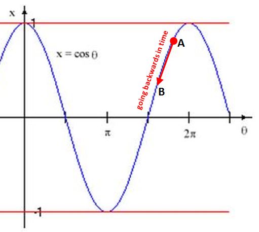
What about electrons? Are they like gyros rotating around some pivot? Here the answer is very simple and very straightforward: No, not at all! First, there are no pivots in an atom. Second, the current understanding of an electron – i.e. the quantum-mechanical understanding of a electron – is not compatible with the classical notion of spin. Let me just copy an explanation from Georgia State University’s HyperPhyics website. It basically says it all:

“Experimental evidence like the hydrogen fine structure and the Stern-Gerlach experiment suggest that an electron has an intrinsic angular momentum, independent of its orbital angular momentum. These experiments suggest just two possible states for this angular momentum, and following the pattern of quantized angular momentum, this requires an angular momentum quantum number of 1/2. With this evidence, we say that the electron has spin 1/2. An angular momentum and a magnetic moment could indeed arise from a spinning sphere of charge, but this classical picture cannot fit the size or quantized nature of the electron spin. The property called electron spin must be considered to be a quantum concept without detailed classical analogy.”

So… I guess this should conclude my exposé on rotational motion. I am not sure what I am going to write about next, but I’ll see. 🙂

Post scriptum:

The above treatment is largely based on Feynman’s Lectures.(Vol. I, Chapter 18, 19 and 20). The subject could also be discussed using the concept of a force couple, aka pure moment. A force couple is a system of forces with a resultant moment but no resultant force. Hence, it causes rotation without translation or, more generally, without any acceleration of the centre of mass. In such analysis, we can say that gravity produces a force couple on the spinning top. The two forces of this couple are equal and opposite, and they pull at opposite ends. However, because one end of the top is fixed (friction forces keep the tip fixed to the ground), the force at the other end makes the top go about the vertical axis.

The situation we have is that gravity causes such force couple to appear, just like the man tilting the spinning wheel causes such force couple to appear. Now, the analysis above shows that the direction of the new force is perpendicular to the plane in which the axis of rotation changes, or wants to change in the case of our spinning top. So gravity wants to pull the top down and causes it to move sideways. This horizontal movement will, in turn, create another force couple. The direction of the resultant force, at the free end of the axis of rotation of the top, will, once again, be vertical, but it will oppose the gravity force. So, in a very simplified explanation of things, we could say:

Gravity pulls the top downwards, and causes a force that will make the top move sideways. So the new force, which causes the precession movement, is orthogonal to the gravitation force, i.e. it’s a horizontal force.
That horizontal force will, in turn, cause another force to appear. That force will also be orthogonal to the horizontal force. As we made two 90 degrees turns, so to say, i.e. 180 degrees in total, it means that this third force will be opposite to the gravitational force.
In equilibrium, we have three forces: gravity, the force causing the precession and, finally, a force neutralizing gravity as the spinning top precesses about the vertical axis.

This approach allows for a treatment that is somewhat more intuitive than Feynman’s concept of the ‘missing force.’

Some content on this page was disabled on June 16, 2020 as a result of a DMCA takedown notice from The California Institute of Technology. You can learn more about the DMCA here:

https://wordpress.com/support/copyright-and-the-dmca/
Some content on this page was disabled on June 16, 2020 as a result of a DMCA takedown notice from The California Institute of Technology. You can learn more about the DMCA here:

https://wordpress.com/support/copyright-and-the-dmca/
Some content on this page was disabled on June 16, 2020 as a result of a DMCA takedown notice from The California Institute of Technology. You can learn more about the DMCA here:

https://wordpress.com/support/copyright-and-the-dmca/
Some content on this page was disabled on June 16, 2020 as a result of a DMCA takedown notice from The California Institute of Technology. You can learn more about the DMCA here:

https://wordpress.com/support/copyright-and-the-dmca/

Spinning: the essentials

Pre-scriptum (dated 26 June 2020): These posts on elementary math and physics have not suffered much (if at all) from the attack by the dark force—which is good because I still like them. While my views on the true nature of light, matter and the force or forces that act on them have evolved significantly as part of my explorations of a more realist (classical) explanation of quantum mechanics, I think most (if not all) of the analysis in this post remains valid and fun to read. In fact, I find the simplest stuff is often the best. 🙂

Original post:

When introducing mirror symmetry (P-symmetry) in one of my older posts (time reversal and CPT-symmetry), I also introduced the concept of axial and polar vectors in physics. Axial vectors have to do with rotations, or spinning objects. Because spin – i.e. turning motion – is such an important concept in physics, I’d suggest we re-visit the topic here.

Of course, I should be clear from the outset that the discussion below is entirely classical. Indeed, as Wikipedia puts it: “The intrinsic spin of elementary particles (such as electrons) is quantum-mechanical phenomenon that does not have a counterpart in classical mechanics, despite the term spin being reminiscent of classical phenomena such as a planet spinning on its axis.” Nevertheless, if we don’t understand what spin is in the classical world – i.e. our world for all practical purposes – then we won’t get even near to appreciating what it might be in the quantum-mechanical world. Besides, it’s just plain fun: I am sure you have played, as a kid of as an adult even, with one of those magical spinning tops or toy gyroscopes and so you probably wonder how it really works in physics. So that’s what this post is all about.

The essential concept is the concept of torque. For rotations in space (i.e. rotational motion), the torque is what the force is for linear motion:

It’s the torque (τ) that makes an object spin faster or slower, just like the force would accelerate or decelerate that very same object when it would be moving along some curve (as opposed to spinning around some axis).
There’s also a similar ‘law of Newton’ for torque: you’ll remember that the force equals the time rate-of-change of a vector quantity referred to as (linear) momentum: F = dp/dt = d(mv)/dt = ma (the mass times the acceleration). Likewise, we have a vector quantity that is referred to as angular momentum (L), and we can write: τ (i.e. the Greek tau) = dL/dt.
Finally, instead of linear velocity, we’ll have an angular velocity ω (omega), which is the time rate-of-change of the angle θ defining how far the object has gone around (as opposed to the distance in linear dynamics, describing how far the object has gone along). So we have ω = dθ/dt. This is actually easy to visualize because we know that θ is the length of the corresponding arc on the unit circle. Hence, the equivalence with the linear distance traveled is easily ascertained.

There are numerous other equivalences. For example, we also have an angular acceleration: α = dω/dt = d²θ/dt²; and we should also note that, just like the force, the torque is doing work – in its conventional definition as used in physics – as it turns an object:

ΔW = τ·Δθ

However, we also need to point out the differences. The animation below does that very well, as it relates the ‘new’ concepts – i.e. torque and angular momentum – to the ‘old’ concepts – i.e. force and linear momentum.

So what do we have here? We have vector quantities once again, denoted by symbols in bold-face. However, τ, L and ω are special vectors: axial vectors indeed, as opposed to the polar vectors F, p and v. Axial vectors are directed along the axis of spin – so that is, strangely enough, at right angles to the direction of spin, or perpendicular to the ‘plane of the twist’ as Feynman calls it – and the direction of the axial vector is determined by the direction of spin through one of two conventions: the ‘right-hand screw rule’ or the ‘left-hand screw rule’. Physicists have settled on the former.

If you feel very confused now (I did when I first looked at it), just step back and go through the full argument as I develop it here. It helps to think of torque (also known, for some obscure reason, as the moment of the force) as a twist on an object or a plane indeed: the torque’s magnitude is equal to the tangential component of the force, i.e. F·sin(Δθ), times the distance between the object and the axis of rotation (we’ll denote this distance by r). This quantity is also equal to the product of the magnitude of the force itself and the length of the so-called lever arm, i.e. the perpendicular distance from the axis to the line of action of the force (this lever arm length is denoted by r₀). So we can write τ as:

The product of the tangential component of the force times the distance r: τ = r·F_t = r·F·sin(Δθ)
The product of the length of the lever arm times the force: τ = r₀·F
The torque is the work done per unit of distance traveled: τ = ΔW/Δθ or τ = dW/dθ in the limit.

So… These are actually only the basics, which you should remember from your high-school physics course. If not, have another look at it. We now need to go from scalar quantities to vector quantities to understand that animation above. Torque is not a vector like force or velocity, not a priori at least. However, we can associate torque with a vector of a special type, an axial vector. Feynman calls vectors such as force or (linear) velocity ‘honest’ or ‘real’ vectors. The mathematically correct term for such ‘honest’ or ‘real’ vectors is polar vector. Hence, axial vectors are not ‘honest’ or ‘real’ in some sense: we derive them from the polar vectors. They are, in effect, a so-called cross product of two ‘honest’ vectors. Here we need to explain the difference between a dot and a cross product between two vectors once again:

(1) A dot product, which we denoted by a little dot (·), yields a scalar quantity: a·b = |a||b|cosα = a·b·cosα with α the angle between the two vectors a and b. Note that the dot product of two orthogonal vectors is equal to zero, so take care: τ = r·F_t = r·F·sin(Δθ) is not a dot product of two vectors. It’s a simple product of two scalar quantities: we only use the dot as a mark of separation, which may be quite confusing. In fact, some authors use ∗ for a product of scalars to avoid confusion: that’s not a bad idea, but it’s not a convention as yet. Omitting the dot when multiplying scalars (as I do when I write |a||b|cosα) is also possible, but it makes it a bit difficult to read formulas I find. Also note, once again, how important the difference between bold-face and normal type is in formulas like this: it distinguishes vectors from scalars – and these are two very different things indeed.

(2) A cross product, which we denote by using a cross (×), yields another vector: τ = r×F =|r|·|F|·sinα·n = r·F·sinα·n with n the normal unit vector given by the right-hand rule. Note how a cross product involves a sine, not a cosine – as opposed to a dot product. Hence, if r and F are orthogonal vectors (which is not unlikely), then this sine term will be equal to 1. If the two vectors are not perpendicular to each other, then the sine function will assure that we use the tangential component of the force.

But, again, how do we go from torque as a scalar quantity (τ = r·F_t) to the vector τ = r×F? Well… Let’s suppose, first, that, in our (inertial) frame of reference, we have some object spinning around the z-axis only. In other words, it spins in the xy-plane only. So we have a torque around (or about) the z-axis, i.e. in the xy-plane. The work that will be done by this torque can be written as:

ΔW = F_xΔx + F_yΔy = (xF_y – yF_x)Δθ

Huh? Yes. This results from a simple two-dimensional analysis of what’s going on in the xy-plane: the force has an x- and a y-component, and the distance traveled in the x- and y-direction is Δx = –yΔθ and Δy = xΔθ respectively. I won’t go into the details of this (you can easily find these elsewhere) but just note the minus sign for Δx and the way the x and y get switched in the expressions.

So the torque in the xy-plane is given by τ_xy = ΔW/Δθ = xF_y – yF_x. Likewise, if the object would be spinning about the x-axis – or, what amounts to the same, in the yz-plane – we’d get τ_yz = yF_z – zF_y. Finally, for some object spinning about the y-axis (i.e. in the zx-plane – and please note I write zx, not xz, so as to be consistent as we switch the order of the x, y and z coordinates in the formulas), then we’d get τ_zx = zF_x – xF_z. Now we can appreciate the fact that a torque in some other plane, at some angle with our Cartesian planes, would be some combination of these three torques, so we’d write:

(1) τ_xy = xF_y – yF_x

(2) τ_yz = yF_z – zF_y and

(3) τ_zx = zF_x – xF_z.

Another observer with his Cartesian x’, y’ and z’ axes in some other direction (we’re not talking some observer moving away from us but, quite simply, a reference frame that’s being rotated itself around some axis not necessarily coinciding with any of the x-, y- z- or x’-, y’- and z’-axes mentioned above) would find other values as he calculates these torques, but the formulas would look the same:

(1’) τ_x’y’ = x’F_y’ – y’F_x’

(2’) τ_y’z’ = y’F_z’ – z’F_y’ and

(3’) τ_z’x’ = z’F_x’ – x’F_z’.

Now, of course, there must be some ‘nice’ relationship that expresses the τ_x’y’, τ_y’z’ and τ_z’x’ values in terms of τ_xy, τ_yz, just like there was some ‘nice’ relationship between the x’, y’ and z’ components of a vector in one coordination system (the x’, y’ and z’ coordinate system) and the x, y, z components of that same vector in the x, y and z coordinate system. Now, I won’t go into the details but that ‘nice’ relationship is, in fact, given by transformation expressions involving a rotation matrix. I won’t write that one down here, because it looks pretty formidable, but just google ‘axis-angle representation of a rotation’ and you’ll get all the details you want.

The point to note is that, in both sets of equations above, we have an x-, y- and z-component of some mathematical vector that transform just like a ‘real’ vector. Now, if it behaves like a vector, we’ll just call it a vector, and that’s how, in essence, we define torque, angular momentum (and angular velocity too) as axial vectors. We should note how it works exactly though:

(1) τ_xy and τ_x’y’ will transform like the z-component of a vector (note that we were talking rotational motion about the z-axis when introducing this quantity);

(2) τ_yz and τ_y’z’ will transform like the x-component of a vector (note that we were talking rotational motion about the x-axis when introducing this quantity);

(3) τ_zx and τ_z’x’ will transform like the y-component of a vector (note that we were talking rotation motion when introducing this quantity). So we have

τ = (τ_yz, τ_zx, τ_xy) = (τ_x, τ_y, τ_z) with

τ_x = τ_yz = yF_z – zF_y

τ_y = τ_zx = zF_x – xF_z

τ_z = τ_xy = xF_y – yF_x.

[This may look very difficult to remember but just look at the order: all we do is respect the clockwise order x, y, z, x, y, z, x, etc. when jotting down the x, y and z subscripts.]

Now we are, finally, well equipped to once again look at that vector representation of rotation. I reproduce it once again below so you don’t have to scroll back to that animation:

We have rotation in the zx-plane here (i.e. rotation about the y-axis) driven by an oscillating force F, and so, yes, we can see that the torque vector oscillates along the y-axis only: its x- and z-components are zero. We also have L here, the angular momentum. That’s a vector quantity as well. We can write it as

L = (L_yz, L_zx, L_xy) = (L_x, L_y, L_z) with

L_x = L_yz = yp_z – zp_y (i.e. the angular momentum about the x-axis)

L_y = L_zx = zp_x – xp_z(i.e. the angular momentum about the y-axis)

L_z = L_xy = xp_y – yp_x (i.e. the angular momentum about the z-axis),

And we note, once again, that only the y-component is non-zero in this case, because the rotation is about the y-axis.

We should now remember the rules for a cross product. Above, we wrote that τ = r´F =|r|×|F|×sina×n = = r×F×sina×n with n the normal unit vector given by the right-hand rule. However, a vector product can also be written in terms of its components: c = a´b if and only

c_x = a_yb_z – a_zb_y,

c_y = a_zb_x – a_xb_z, and

c_z = a_xb_y – a_yb_x.

Again, if this looks difficult, remember the trick above: respect the clockwise order when jotting down the x, y and z subscripts. I’ll leave it to you to work out r´F and r´p in terms of components but, when you write it all out, you’ll see it corresponds to the formulas above. In addition, I will also leave it to you to show that the velocity of some particle in a rotating body can be given by a similar vector product: v = ω´r, with ω being defined as another axial vector (aka pseudovector) pointing along the direction of the axis of rotation, i.e. not in the direction of motion. [Is that strange? No. As it’s rotational motion, there is no ‘direction of motion’ really: the object, or any particle in that object, goes round and round and round indeed and, hence, defining some normal vector using the right-hand rule to denote angular velocity makes a lot of sense.]

I could continue to write and write and write, but I need to stop here. Indeed, I actually wanted to tell you how gyroscopes work, but I notice that this introduction has already taken several pages. Hence, I’ll leave the gyroscope for a separate post. So, be warned, you’ll need to read and understand this one before reading my next one.

On (special) relativity: what’s relative?

Pre-scriptum (dated 26 June 2020): These posts on elementary math and physics have not suffered much the attack by the dark force—which is good because I still like them. While my views on the true nature of light, matter and the force or forces that act on them have evolved significantly as part of my explorations of a more realist (classical) explanation of quantum mechanics, I think most (if not all) of the analysis in this post remains valid and fun to read. In fact, I find the simplest stuff is often the best. 🙂

Original post:

This is my third and final post about special relativity. In the previous posts, I introduced the general idea and the Lorentz transformations. I present these Lorentz transformations once again below, next to their Galilean counterparts. [Note that I continue to assume, for simplicity, that the two reference frames move with respect to each other along the x- axis only, so the y- and z-component of u is zero. It is not all that difficult to generalize to three dimensions (especially not when using vectors) but it makes an intuitive understanding of what’s relativity all about more difficult.]

As you can see, under a Lorentz transformation, the new ‘primed’ space and time coordinates are a mixture of the ‘unprimed’ ones. Indeed, the new x’ is a mixture of x and t, and the new t’ is a mixture as well. You don’t have that under a Galilean transformation: in the Newtonian world, space and time are neatly separated, and time is absolute, i.e. it is the same regardless of the reference frame. In Einstein’s world – our world – that’s not the case: time is relative, or local as Hendrik Lorentz termed it, and so it’s space-time – i.e. ‘some kind of union of space and time’ as Minkowski termed it – that transforms. In practice, physicists will use so-called four-vectors, i.e. vectors with four coordinates, to keep track of things. These four-vectors incorporate both the three-dimensional space vector as well as the time dimension. However, we won’t go into the mathematical details of that here.

What else is relative? Everything, except the speed of light. Of course, velocity is relative, just like in the Newtonian world, but the equation to go from a velocity as measured in one reference frame to a velocity as measured in the other, is different: it’s not a matter of just adding or subtracting speeds. In addition, besides time, mass becomes a relative concept as well in Einstein’s world, and that was definitely not the case in the Newtonian world.

What about energy? Well… We mentioned that velocities are relative in the Newtonian world as well, so momentum and kinetic energy were relative in that world as well: what you would measure for those two quantities would depend on your reference frame as well. However, here also, we get a different formula now. In addition, we have this weird equivalence between mass and energy in Einstein’s world, about which I should also say something more.

But let’s tackle these topics one by one. We’ll start with velocities.

Relativistic velocity

In the Newtonian world, it was easy. From the Galilean transformation equations above, it’s easy to see that

v’ = dx’/dt’ = d(x – ut)/dt = dx/dt – d(ut)/dt = v – u

So, in the Newtonian world, it’s just a matter of adding/subtracting speeds indeed: if my car goes 100 km/h (v), and yours goes 120 km/h, then you will see my car falling behind at a speed of (minus) 20 km/h. That’s it. In Einstein’s world, it is not so simply. Let’s take the spaceship example once again. So we have a man on the ground (the inertial or ‘unprimed’ reference frame) and a man in the spaceship (the primed reference frame), which is moving away from us with velocity u.

Now, suppose an object is moving inside the spaceship (along the x-axis as well) with a (uniform) velocity v_x’, as measured from the point of view of the man inside the spaceship. Then the displacement x’ will be equal to x’ = v_x’t’. To know how that looks from the man on the ground, we just need to use the opposite Lorentz transformations: just replace u by –u everywhere (to the man in the spaceship, it’s like the man on the ground moves away with velocity –u), and note that the Lorentz factor does not change because we’re squaring and (–u)²= u². So we get:

Hence, x’ = v_x’t’ can be written as x = γ(v_x’t’ + ut’). Now we should also substitute t’, because we want to measure everything from the point of view of the man on the ground. Now, t = γ(t’ + uv_x’t’/c²). Because we’re talking uniform velocities, v_x(i.e. the velocity of the object as measured by the man on the ground) will be equal to x divided by t (so we don’t need to take the time derivative of x), and then, after some simplifying and re-arranging (note, for instance, how the t’ factor miraculously disappears), we get:

What does this rather complicated formula say? Just put in some numbers:

Suppose the object is moving at half the speed of light, so 0.5c, and that the spaceship is moving itself also at 0.5c, then we get the rather remarkable result that, from the point of view of the observer on the ground, that object is not going as fast as light, but only at v_x = (0.5c + 0.5c)/(1 + 0.5·0.5) = 0.8c.
Or suppose we’re looking at a light beam inside the spaceship, so something that’s traveling at speed c itself in the spaceship. How does that look to the man on the ground? Just put in the numbers: v_x = (0.5c + c)/(1 + 0.5·1) = c ! So the speed of light is not dependent on the reference frame: it looks the same – both to the man in the ship as well as to the man on the ground. As Feynman puts it: “This is good, for it is, in fact, what the Einstein theory of relativity was designed to do in the first place–so it had better work!”

It’s interesting to note that, even if u has no y– or z-component, velocity in the y direction will be affected too. Indeed, if an object is moving upward in the spaceship, then the distance of travel of that object to the man on the ground will appear to be larger. See the triangle below: if that object travels a distance Δs’ = Δy’ = Δy = v’Δt’ with respect to the man in the spaceship, then it will have traveled a distance Δs = vΔt to the man on the ground, and that distance is longer.

I won’t go through the process of substituting and combining the Lorentz equations (you can do that yourself) but the grand result is the following:

v_y = (1/γ)v_y’

1/γ is the reciprocal of the Lorentz factor, and I’ll leave it to you to work out a few numeric examples. When you do that, you’ll find the rather remarkable result that v_y is actually less than v_y’. For example, for u = 0.6c, 1/γ will be equal to 0.8, so v_y will be 20% less than v_y’. How is that possible? The vertical distance is what it is (Δy’ = Δy), and that distance is not affected by the ‘length contraction’ effect (y’ = y). So how can the vertical velocity be smaller? The answer is easy to state, but not so easy to understand: it’s the time dilation effect: time in the spaceship goes slower. Hence, the object will cover the same vertical distance indeed – for both observers – but, from the point of view of the observer on the ground, the object will apparently need more time to cover that distance than the time measured by the man in the spaceship: Δt > Δt’. Hence, the logical conclusion is that the vertical velocity of that object will appear to be less to the observer on the ground.

How much less? The time dilation factor is the Lorentz factor. Hence, Δt = γΔt’. Now, if u = 0.6c, then γ will be equal to 1.25 and Δt = 1.25Δt’. Hence, if that object would need, say, one second to cover that vertical distance, then, from the point of view of the observer on the ground, it would need 1.25 seconds to cover the same distance. Hence, its speed as observed from the ground is indeed only 1/(5/4) = 4/5 = 0.8 of its speed as observed by the man in the spaceship.

Is that hard to understand? Maybe. You have to think through it. One common mistake is that people think that length contraction and/or time dilation are, somehow, related to the fact that we are looking at things from a distance and that light needs time to reach us. Indeed, on the Web, you can find complicated calculations using the angle of view and/or the line of sight (and tons of trigonometric formulas) as, for example, shown in the drawing below. These have nothing to do with relativity theory and you’ll never get the Lorentz transformation out of them. They are plain nonsense: they are rooted in an inability of these youthful authors to go beyond Galilean relativity. Length contraction and/or time dilation are not some kind of visual trick or illusion. If you want to see how one can derive the Lorentz factor geometrically, you should look for a good description of the Michelson-Morley experiment in a good physics handbook such as, yes :-), Feynman’s Lectures.

So, I repeat: illustrations that try to explain length contraction and time dilation in terms of line of sight and/or angle of view are useless and will not help you to understand relativity. On the contrary, they will only confuse you. I will let you think through this and move on to the next topic.

Relativistic mass and relativistic momentum

Einstein actually stated two principles in his (special) relativity theory:

The first is the Principle of Relativity itself, which is basically just the same as Newton’s principle of relativity. So that was nothing new actually: “If a system of coordinates K is chosen such that, in relation to it, physical laws hold good in their simplest form, then the same laws must hold good in relation to any other system of coordinates K’ moving in uniform translation relatively to K.” Hence, Einstein did not change the principle of relativity – quite on the contrary: he re-confirmed it – but he did change Newton’s Laws, as well as the Galilean transformation equations that came with them. He also introduced a new ‘law’, which is stated in the second ‘principle’, and that the more revolutionary one really:
The Principle of Invariant Light Speed: “Light is always propagated in empty space with a definite velocity [speed] c which is independent of the state of motion of the emitting body.”

As mentioned above, the most notable change in Newton’s Laws – the only change, in fact – is Einstein’s relativistic formula for mass:

m_v = γm₀

This formula implies that the inertia of an object, i.e. its mass, also depends on the reference frame of the observer. If the object moves (but velocity is relative as we know: an object will not be moving if we move with it), then its mass increases. This affects its momentum. As you may or may not remember, the momentum of an object is the product of its mass and its velocity. It’s a vector quantity and, hence, momentum has not only a magnitude but also a direction:

p_v = m_vv = γm₀v

As evidenced from the formula above, the momentum formula is a relativistic formula as well, as it’s dependent on the Lorentz factor too. So where do I want to go from here? Well… In this section (relativistic mass and momentum), I just want to show that Einstein’s mass formula is not some separate law or postulate: it just comes with the Lorentz transformation equations (and the above-mentioned consequences in terms of measuring horizontal and vertical velocities).

Indeed, Einstein’s relativistic mass formula can be derived from the momentum conservation principle, which is one of the ‘physical laws’ that Einstein refers to. Look at the elastic collision between two billiard balls below. These balls are equal – same mass and same speed from the point of view of an inertial observer – but not identical: one is red and one is blue. The two diagrams show the collision from two different points of view: left, we have the inertial reference frame, and, right, we have a reference frame that is moving with a velocity equal to the horizontal component of the velocity of the blue ball.

The points to note are the following:

The total momentum of such elastic collision before and after the collision must be the same.
Because the two balls have equal mass (in the inertial reference frame at least), the collision will be perfectly symmetrical. Indeed, we may just turn the diagram ‘upside down’ and change the colors of the balls, as we do below, and the values w, u and v (as well as the angle α) are the same.

As mentioned above, the velocity of the blue and red ball and, hence, their momentum, will depend on the frame of reference. In the diagram on the left, we’re moving with a velocity equal to the horizontal component of the velocity of the blue ball and, therefore, in this particular frame of reference, the velocity (and the momentum) of the blue ball consists of a vertical component only, which we refer to as w.

From this point of view (i.e. the reference frame moving with, the velocity (and, hence, the momentum) of the red ball will have both a horizontal as well as a vertical component. If we denote the horizontal component by u, then it’s easy to show that the vertical velocity of the red ball must be equal to sin(α)v. Now, because u = cos(α)v, this vertical component will be equal to tan(α)u. But so what is tan(α)u? Now, you’ll say, that is quite evident: tan(α)u must be equal to w, right?

No. That’s Newtonian physics. The red ball is moving horizontally with speed u with respect to the blue ball and, hence, its vertical velocity will not be quite equal to w. Its vertical velocity will be given by the formula which we derived above: v_y = (1/γ)v_y’, so it will be a little bit slower than the w we see in the diagram on the right which is, of course, the same w as in the diagram on the left. [If you look carefully at my drawing above, then you’ll notice that the w vector is a bit longer indeed.]

Huh? Yes. Just think about it: tan(α)u = (1/γ)w. But then… How can momentum be conserved if these speeds are not the same? Isn’t the momentum conservation principle supposed to conserve both horizontal as well as vertical momentum? It is, and momentum is being conserved. Why? Because of the relativistic mass factor.

Indeed, the change in vertical momentum (Δp) of the blue ball in the diagram on the left or – which amounts to the same – the red ball in the diagram on the right (i.e. the vertically moving ball) is equal to Δp_blue = 2m_ww. [The factor 2 is there because the ball goes down and then up (or vice versa) and, hence, the total change in momentum must be twice the m_ww amount.] Now, that amount must be equal to Δp_red, which is equal to Δp_blue = 2m_v(1/γ)w. Equating both yields the following grand result:

m_v/m_w= γ ⇔ m_v= γm_w

What does this mean? It means that mass of the red ball in the diagram on the left is larger than the mass of the blue ball. So here we have actually derived Einstein’s relativistic mass formula from the momentum conservation principle !

Of course you’ll say: not quite. This formula is not the m_u= γm₀formula that we’re used to ! Indeed, it’s not. The blue ball has some velocity w itself, and so the formula links two velocities v and w. However, we can derive m_v= γm₀formula as a limit of m_v= γm_w for w going to zer0. How can w become infinitesimally small? If the angle α becomes infinitesimally small. It’s obvious, then, that v and u will be practically equal. In fact, if w goes to zero, then m_wwill be equal to m₀in the limiting case, and m_vwill be equal to m_u. So, then, indeed, we get the familiar formula as a limiting case:

m_u= γm₀

Hmm… You’ll probably find all of this quite fishy. I’d suggest you just think about it. What I presented above, is actually Feynman’s presentation of the subject, but with a bit more verbosity. Let’s move on to the final.

Relativistic energy

From what I wrote above (and from what I wrote in my two previous posts on this topic), it should be obvious, by now, that energy also depends on the reference frame. Indeed, mass and velocity depend on the reference frame (moving or not), and both appear in the formula for kinetic energy which, as you’ll remember, is

K.E. = mc²– m₀c²= (m – m₀)c²= γm₀c²– m₀c²= m₀c²(γ – 1).

Now, if you go back to the post where I presented that formula, you’ll see that we’re actually talking the change in kinetic energy here: if the mass is at rest, it’s kinetic energy is zero (because m = m₀), and it’s only when the mass is moving, that we can observe the increase in mass. [If you wonder how, think about the example of the fast-moving electrons in an electron beam: we see it as an increase in the inertia: applying the same force does no longer yield the same acceleration.]

Now, in that same post, I also noted that Einstein added an equivalent rest mass energy (E₀= m₀c²) to the kinetic energy above, to arrive at the total energy of an object:

E = E₀+ K.E. = mc²

Now, what does this equivalence actually mean? Is mass energy? Can we equate them really? The short answer to that is: yes.

Indeed, in one of my older posts (Loose Ends), I explained that protons and neutrons are made of quarks and, hence, that quarks are the actual matter particles, not protons and neutrons. However, the mass of a proton – which consists of two up quarks and one down quark – is 938 MeV/c²(don’t worry about the units I am using here: because protons are so tiny, we don’t measure their mass in grams), but the mass figure you get when you add the rest mass of two u‘s and one d, is 9.6 MeV/c²only: about one percent of 938 ! So where’s the difference?

The difference is the equivalent mass (or inertia) of the binding energy between the quarks. Indeed, the so-called ‘mass’ that gets converted into energy when a nuclear bomb explodes is not the mass of quarks. Quarks survive: nuclear power is binding energy between quarks that gets converted into heat and radiation and kinetic energy and whatever else a nuclear explosion unleashes.

In short, 99% of the ‘mass’ of a proton or an electron is due to the strong force. So that’s ‘potential’ energy that gets unleashed in a nuclear chain reaction. In other words, the rest mass of the proton is actually the inertia of the system of moving quarks and gluons that make up the particle. In such atomic system, even the energy of massless particles (e.g. the virtual photons that are being exchanged between the nucleus and its electron shells) is measured as part of the rest mass of the system. So, yes, mass is energy. As Feynman put it, long before the quark model was confirmed and generally accepted:

“We do not have to know what things are made of inside; we cannot and need not justify, inside a particle, which of the energy is rest energy of the parts into which it is going to disintegrate. It is not convenient and often not possible to separate the total mc²energy of an object into (1) rest energy of the inside pieces, (2) kinetic energy of the pieces, and (3) potential energy of the pieces; instead we simply speak of the total energy of the particle. We ‘shift the origin’ of energy by adding a constant m₀c²to everything, and say that the total energy of a particle is the mass in motion times c², and when the object is standing still, the energy is the mass at rest times c².” (Richard Feynman’s Lectures on Physics, Vol. I, p. 16-9)

So that says it all, I guess, and, hence, that concludes my little ‘series’ on (special) relativity. I hope you enjoyed it.

Post scriptum:

Feynman describes the concept of space-time with a nice analogy: “When we move to a new position, our brain immediately recalculates the true width and depth of an object from the ‘apparent’ width and depth. But our brain does not immediately recalculate coordinates and time when we move at high speed, because we have had no effective experience of going nearly as fast as light to appreciate the fact that time and space are also of the same nature. It is as though we were always stuck in the position of having to look at just the width of something, not being able to move our heads appreciably one way or the other; if we could, we understand now, we would see some of the other man’s time—we would see “behind”, so to speak, a little bit. Thus, we shall try to think of objects in a new kind of world, of space and time mixed together, in the same sense that the objects in our ordinary space-world are real, and can be looked at from different directions. We shall then consider that objects occupying space and lasting for a certain length of time occupy a kind of a “blob” in a new kind of world, and that when we look at this “blob” from different points of view when we are moving at different velocities. This new world, this geometrical entity in which the “blobs” exist by occupying position and taking up a certain amount of time, is called space-time.”

If none of what I wrote could convey the general idea, then I hope the above quote will. 🙂 Apart from that, I should also note that physicists will prefer to re-write the Lorentz transformation equations by measuring time and distance in so-called equivalent units: velocities will be expressed not in km/h but as a ratio of c and, hence, c = 1 (a pure number) and so u will also be a pure number between 0 and 1. That can be done by expressing distance in light-seconds ( a light-second is the distance traveled by light in one second or, alternatively, by expressing time in ‘meter’. Both are equivalent but, in most textbooks, it will be time that will be measured in the ‘new’ units. So how do we express time in meter?

It’s quite simple: we multiply the old seconds with c and then we get: time_{expressed in meters}= time_{expressed in seconds}multiplied by 3×10⁸meters per second. Hence, as the ‘second’ the first factor and the ‘per second’ in the second factor cancel out, the dimension of the new time unit will effectively be the meter. Now, if both time and distance are expressed in meter, then velocity becomes a pure number without any dimension, because we are dividing distance expressed in meter by time expressed in meter, and it should be noted that it will be a pure number between 0 and 1 (0 ≤ u ≤ 1), because 1 ‘time second’ = 1/(3×10⁸) ‘time meters’. Also, c itself becomes the pure number 1. The Lorentz transformation equations then become:

They are easy to remember in this form (cf. the symmetry between x – ut and t – ux) and, if needed, we can always convert back to the old units to recover the original formulas.

I personally think there is no better way to illustrate how space and time are ‘mere shadows’ of the same thing indeed: if we express both time and space in the same dimension (meter), we can see how, as result of that, velocity becomes a dimensionless number between zero and one and, more importantly, how the equations for x’ and t’ then mirror each other nicely. I am not sure what ‘kind of union’ between space and time Minkowski had in mind, but this must come pretty close, no?

Final note: I noted the equivalence of mass and energy above. In fact, mass and energy can also be expressed in the same units, and we actually do that above already. If we say that an electron has a rest mass of 0.511 MeV/c²(a bit less than a quarter of the mass of the u quark), then we express the mass in terms of energy. Indeed, the eV is an energy unit and so we’re actually using the m = E/c² formula when we express mass in such units. Expressing mass and energy in equivalent units allows us to derive similar ‘Lorentz transformation equations’ for the energy and the momentum of an object as measured under an inertial versus a moving reference frame. Hence, energy and momentum also transform like our space-time four-vectors and – likewise – the energy and the momentum itself, i.e. the components of the (four-)vector, are less ‘real’ than the vector itself. However, I think this post has become way too long and, hence, I’ll just jot these four equations down – please note, once again, the nice symmetry between (1) and (2) – but then leave it at that and finish this post. 🙂

On (special) relativity: the Lorentz transformations

Original post:

I just skyped to my kids (unfortunately, we’re separated by circumstances) and they did not quite get the two previous posts (on energy and (special) relativity). The main obstacle is that they don’t know much – nothing at all actually – about integrals. So I should avoid integrals. That’s hard but I’ll try to do so in this post, in which I want to introduce special relativity as it’s usually done, and so that’s not by talking about Einstein’s mass-energy equivalence relation first.

Galilean/Newtonian relativity

A lot of people think they understand relativity theory but they often confuse it with Galilean (aka Newtonian) relativity and, hence, they actually do not understand it at all. Indeed, Galilean or Newtonian relativity is as old as Galileo and Newton (so that’s like 400 years old), who stated the principle of relativity as a corollary to the laws of motion: “The motions of bodies included in a given space are the same amongst themselves, whether that space is at rest or moves uniformly forward in a straight line.”

The Galilean or Newtonian principle of relativity is about adding and subtracting speeds: if I am driving at 120 km/h on some highway, but you overtake me at 140 km/h, then I will see you go past me at the rather modest speed of 20 km/h. That’s all what there is to it.

Now, that’s not what Einstein‘s relativity theory is about. Indeed, the relationship between your and my reference frame (yours is moving with respect to mine, and mine is moving with respect to yours but with opposite velocity) is very simple in this example. It involves a so-called Galilean transformation only: if my coordinate system is (x, y, z, t), and yours is (x‘, y‘, z‘, t‘), then we can write:

(1) x’ = x – ut (or x = x’ + ut), (2) y’ = y, (3) z’ = z and (4) t’ = t

To continue the example above: if we start counting at t = t’ = 0 when you are overtaking me, and if we both consider ourselves to be at the center of our reference frame (i.e. x = 0 where I am and x’ = 0 where you are), then you will be at x = 10 km after 30 minutes from my point of view, and I will be at x’ = –10 km (so that’s 10 km behind) from your point of view. So x’ = x – ut indeed, with u = 20 km/h.

Again, that’s not what Einstein’s principle of relativity is about. They knew that very well in the 17th century already. In fact, they actually knew that much earlier but Descartes formalized his Cartesian coordinate system only in the first half of the 17th century and, hence, it’s only from that time onwards that scientists such as Newton and Huygens started using it to transform the laws of physics from one frame of reference to another. What they found is that those laws remained invariant.

For example, the conservation law for momentum remains valid even if, as illustrated below, an inertial observer will see an elastic collision, such as the one illustrated, differently than a observer who’s moving along: for the observer who’s moving along, the (horizontal) speed of the blue ball will be zero, and the (horizontal) speed of the red ball will be twice the speed as observed by the inertial observer. That being said, both observers will find that momentum (i.e. the product of mass and velocity: p = mv) is being conserved in such collisions.

But, again, that’s Galilean relativity only: the laws of Newton are of the same form in a moving system as in a stationary system and, therefore, it is impossible to tell, by making experiments, whether our system is moving or not. In other words: there is no such thing as ‘absolute speed’. But, so – let me repeat it again – that is not what Einstein’s relativity theory is about.

Let me give a more interesting example of Galilean relativity, and then we can see what’s wrong with it. The speed of a sound wave is not dependent on the motion of the source: the sound of a siren of an ambulance or a noisy car engine will always travel at a speed of 343 meter per second, regardless of the motion of the ambulance. So, while we’ll experience a so-called Doppler effect when the ambulance is moving – i.e. a higher pitch when it’s approaching than when it’s receding – this Doppler effect does not have any impact on the speed of the sound wave. It only affects the frequency as we hear it. The speed of the wave depends on the medium only, i.e. air in this case.

Indeed, the speed of sound will be different in another gas, or in a fluid, or in a solid, and there’s a surprisingly simple function for that – the so-called Newton-Laplace equation: v_sound = (k/ρ)². In this equation, k is a coefficient of ‘stiffness’ of the medium (even if ‘stiffness’ sounds somewhat strange as a concept to apply to gases), and ρ is the density of the medium (so lower or higher air density will increase/decrease the speed of sound).

This has nothing to do with speed being absolute. No. The Galilean relativity principle does come into play, as one would expect: it is actually possible to catch up with a sound wave (or with any wave traveling through some medium). In fact, that’s what supersonic planes do: they catch up with their own sound waves. However, in essence, planes are not any different from cars in terms of their relationship with the sound that they produce. It’s just that they are faster: the sound wave they produce also travels at a speed of 1,235 km/h, and so cars can’t match that, but supersonic planes can!

[As for the shock wave that is being produced as these planes accelerate and actually ‘break’ the ‘sound barrier’, that has to do with the pressure waves the plane creates in front of itself (just like a traveling compresses the air in front of it). These pressure waves also travel at the speed of sound. Now, as the speed of the object increases, the waves are forced together, or compressed, because they cannot get out of the way of each other. Eventually they merge into one single shock wave, and so that’s what happens and creates the ‘sonic boom’, which also travels at the speed of sound. However, that should not concern us here. For more information on this, I’d refer to Wikipedia, as I got these illustrations from that source, and I quite like the way they present the topic.]

The Doppler effect looks somewhat different (it’s illustrated above) but so, once again, this phenomenon has nothing to do with Einstein’s relativity theory. Why not? Because we are still talking Galilean relativity here. Indeed, let’s suppose our plane travels at twice the speed of sound (i.e. Mach 2 or almost 2,500 km/h). For us, as inertial observers, the speed of the sound wave originating at point 0 in the illustration above (i.e. the reference frame of the inertial observer) will be equal to dx/dt = 1235 km/h. However, for the pilot, the speed of that wave will be equal to

dx’/dt = d(x – ut)/dt = dx/dt – d(ut)/dt = dx/dt – d(ut)/dt = 1235 km/h – u

= 1235 km/h – u = 1235 km/h – 2470 km/h = – 1235 km/h

In short, from the point of view of the pilot, he sees the wave front of the wave created at point 0 traveling away from him (cf. the negative value) at 1235 km/h, i.e. the speed of sound. That makes sense obviously, because he travels twice as fast. However – I cannot repeat it enough – this phenomenon has nothing to do with Einstein’s theory of relativity: if they could have imagined supersonic travel, Galileo, Newton and Huygens would have predicted that too.

So what’s Einstein’s theory of (special) relativity about?

Einstein’s principle of relativity

In 1865, the Scottish mathematical physicist James Clerk Maxwell – I guess it’s important to note he’s Scottish with that referendum coming 🙂 – finally discovered that light was nothing but electromagnetic radiation – so radio waves, (visible) light, X-rays, gamma rays,… It’s all the same: electromagnetic radiation, also known as light tout court.

Now, the equations that describe how electromagnetic radiation (i.e. light) travels through space are beautiful but involve operators which you may not recognize and, hence, I will not write them down. The point to note is that Maxwell’s equations were very elegant but… There were two major difficulties with them:

They did not respect Galilean relativity: if we transform them using the above-mentioned Galilean transformation (x’ = x – ut, y’ = y, z’ = z and t’ = t) then we do not get some relative speed of light. On the contrary, according to Maxwell’s equations, from whatever reference frame you look at light, it should always travel at the same (absolute) speed of light c = 299,792 km/h. So c is a constant, and the same constant, ALWAYS.
Scientists did not have any clue about the medium in which light was supposed to travel. The second half of the 19th century saw lots of experiments trying to discover evidence of a hypothetical ‘luminiferous aether’ in which light was supposed to travel, and which should also have some ‘stiffness’ and ‘density’, but so they could not find any trace of it. No one ever did, and so now we’ve finally accepted that light can actually travel in a vacuum, i.e. in plain nothing.

So what? Well… Let’s first look at the first point. Just like a sound wave, the motion of the source does not have any impact on the speed of light: it goes out in all directions at the same speed c, whether it is emitted from a fast-moving car or from some beacon near the sea. However, unlike sound waves, Maxwell’s equations imply that we cannot catch up with them. That’s troublesome, very troublesome, because, according to the above-mentioned Galilean transformation rules,

i.e. v’ = dx’/dt = dx/dt – u = v – u,

some light beam that is traveling at speed v = c past a spaceship that itself is traveling at speed u – let’s say u = 0.2c for example – should have a speed of c‘ = c – 0.2c = 0.8c = = 239,834 km/h only with respect to the spaceship. However, that’s not what Maxwell’s equations say when you substitute x, y, z and t for x‘, y‘, z‘ and t‘ using those four simple equations x’ = x – ut, y’ = y, z’ = z and t’ = t. After you do the substitution, the transformed Maxwell equations will once again yield that c’ = c = 299,792 km/h, and not c’ = 0.8×299,792 km/h = 239,834 km/h.

That’s weird ! Why? Well… If you don’t think that this is weird, then you’re actually not thinking at all ! Just compare it with the example of our sound wave. There is just no logic to it !

The discovery startled all scientists because there could only be possible solutions to the paradox:

Either Maxwell’s equations were wrong (because they did not observe the principle of (Galilean relativity) or, else,
Newton’s equations (and the Galilean transformation rules – i.e. the Galilean relativity principle) are wrong.

Obviously, scientists and experimenters first tried to prove that Maxwell had it all wrong – if only because no experiment had ever shown Newton’s Laws to be wrong, and so it was probably hard – if not impossible – to try to come up with one that would ! So, instead, experimenters invented all kinds of wonderful apparatuses trying to show that the speed of the light was actually not absolute.

Basically, these experiments assumed that the speed of the Earth, as it rotates around the Sun at a speed of 108,000 km per hour, would result in measurable differences of c that would depend on the direction of the apparatus. More specifically, the speed of the light beam, as measured, would be different if the light beam would be traveling parallel to the motion of the Earth, as opposed to the light beam traveling at right angle to the motion of the Earth. Why? Well… It’s the same idea as the car chasing its own light beams, but I’ll refer to you to other descriptions of the experiment, because explaining these set-ups would take too much time and space. 🙂 I’ll just say that, because 108,000 km/h (on average) is only about 30 km per second (i.e. 0.0001 times c), these experiments relied on (expected) interference effects. The technical aspect of these experiments is really quite interesting. However, as mentioned above, I’ll refer you to Wikipedia or other sources if you’d want more detail.

Just note the most famous of those experiments: the 1887 Michelson-Morley experiment, also known as ‘the most famous failed experiment in history’ because, indeed, it failed to find any interference effects: the speed of light always was the speed of light, regardless of the direction of the beam with respect to the direction of motion of the Earth.

The Lorentz transformations

Once the scientists had recovered from this startling news (Michelson himself suffered from a nervous breakdown for a while, because he really wanted to find that interference effect in order to disprove Maxwell’s Laws), they suggested solutions.

The math was solved first. Indeed, just before the turn of the century, the Dutch physicist Hendrik Antoon Lorentz suggested that, if material bodies would contract in the direction of their motion with a factor (1 – u²/c²)^1/2 and, in addition, if time would also be dilated with a factor (1 – u²/c²)^–1/2, then the Michelson-Morley results could be explained. Of course, scientists objected to this ‘explanation’ as being very much ‘ad hoc’.

So then came Einstein. He just took the math for granted, so Einstein basically accepted the so-called Lorentz transformations that resulted from it, and corrected Newton’s Law in order to set physics right again.

And so that was it. As it turned out, all that was needed in fact, was to do away with the assumption that the inertia (or mass) of an object is a constant and, hence, that it does not vary with its velocity. For us, today, it seems obvious: mass also varies, and the factor involved is the very same Lorentz factor that we mentioned above: γ = (1 – u²/c²)^–1/2. Hence, the m in Newton’s Second Law (F = d(mv)/dt) is not a constant but equal to m = γm₀. For all speeds that we, human beings, can imagine (including the astronomical speed of the Earth in orbit around the Sun), the ‘correction’ is too small to be noticeable, or negligible, but so it’s there, as evidenced by the Michelson-Morley experiment, and, some hundred years later, we can actually verify it in particle accelerators.

As said, for us, today, it’s obvious (in my previous post, I mention a few examples: I explain how the mass of electrons in an electron beam is impacted by their speed, and how the lifetime of muon increases because of their speed) but one hundred years ago, it was not. Not at all – and so that’s why Einstein was a genius: he dared to explore and accept the non-obvious.

Now, what then are the correct transformations from one reference frame to another? They are referred to as the Lorentz transformations, and they can be written down (in a simplified form, assuming relative motion in the x direction only) as follows:

Now, I could point out many interesting implications, or come up with examples, but I will resist the temptation. I will only note two things about them:

1. These Lorentz transformations actually re-establish the principle of relativity: the Laws of Nature – including the Laws of Newton as corrected by Einstein’s relativistic mass formula – are of the same form in a moving system as in a stationary system, and therefore it is impossible to tell, by making experiments, whether the system is moving or not.

2. The second thing I should note is that the equations above imply that the idea of absolute time is no longer valid: there is no such thing as ‘absolute’ or ‘universal’ time. Indeed, Lorentz’ concept of ‘local time’ is a most profound departure from Newtonian mechanics that is implicit in these equations.

Indeed, space and time are entangled in these equations as you can see from the –ut and –ux/c² terms in the equation for x’ and t’ respectively and, hence, the idea of simultaneity has to be abandoned: what happens simultaneously in two separated places according to one observer, does not happen at the same time as viewed by an observer moving with respect to the first. Let me quickly show how.

Suppose that in my world I see two events happening at the same time t₀but so they happen at two different places x₁ and x₂. Now, if you are movingaway from me at a (uniform) speed u, then equation (4) tells us that you will see these two events happen at two different times t₁‘ and t₂‘, with the time difference t₁‘ – t₂‘ equal to t₁‘ – t₂‘ = γ[u(x₁ – x₂)/c²], with γ the above-mentioned Lorentz factor. [Just do the calculation for yourself using equation 4.]

Of course, the effect is negligible for most speeds that we, as human beings, can imagine, but it’s there. So we do not have three separate space coordinates and one time coordinates, but four space-time coordinates that transform together, fully entangled, when applying those four equations above.

That observation led the German mathematician Hermann Minkowski, who helped Einstein to develop his theory of four-dimensional space-time, to famously state that “Space of itself, and time of itself, will sink into mere shadows, and only a kind of union between them shall survive.”

Post scriptum: I did not elaborate on the second difficulty when I mentioned Maxwell’s equations: the lack of a need for a medium for light to travel through. I will let that rest for the moment (or, else, you can just Google some stuff on it). Just note that (1) it is kinda convenient that electromagnetic radiation does not need any medium (I can’t see how one would incorporate that in relativity theory) and (2) that light does seem to slow down in a medium. However, the explanation for that (i.e. for light to have an apparently lower speed in a medium) is to be found in quantum mechanics and so we won’t touch upon that complex matter here (for now that is). The point to note is that this slowing down is caused by light interacting with the matter it encounters as it travels through the medium. It does not actually go slower. However, I need to stop here as this is, yet again, a post which has become way too long. On the other hand, I am hopeful my kids will actually understand this one, because it does not involve integrals. 🙂

Another post for my kids: introducing (special) relativity

Original post:

In my previous post, I talked about energy, and I tried to keep it simple – but also accurate. However, to be completely accurate, one must, of course, introduce relativity at some point. So how does that work? What’s ‘relativistic’ energy? Well… Let me try to convey a few ideas here.

The first thing to note is that the energy conservation law still holds: special theory or not, the sum of the kinetic and potential energies in a (closed) system is always equal to some constant C. What constant? That doesn’t matter: Nature does not care about our zero point and, hence, we can add or subtract any (other) constant to the equation K.E. + P.E. = T + U = C.

That being said, in my previous post, I pointed out that the constant depends on the reference point for the potential energy term U: we will usually take infinity as the reference point (for a force that attracts) and associate it with zero potential (U = 0). We then get a function U(x) like the one below: for gravitational energy we have U(x) = –GMm/x, and for electrical charges, we have U(x) = q₁q₂/4πε₀x. The mathematical shape is exactly the same but, in the case of the electromagnetic forces, you have to remember that likes repel, and opposites attract, so we don’t need the minus sign: the sign of the charges takes care of it.

Minus sign? In case you wonder why we need that minus sign for the potential energy function, well… I explained that in my previous post and so I’ll be brief on that here: potential energy is measured by doing work against the force. That’s why. So we have an infinite sum (i.e. an integral) over some trajectory or path looking like this: U = – ∫F·ds.

For kinetic energy, we don’t need any minus sign: as an object picks up speed, it’s the force itself that is doing the work as its potential energy is converted into kinetic energy, so the change in kinetic energy will equal the change in potential energy, but with opposite sign: as the object loses potential energy, it gains kinetic energy. Hence, we write ΔT = –ΔU = ∫F·ds..

That’s all kids stuff obviously. Let’s go beyond this and ask some questions. First, why can we add or subtract any constant to the potential energy but not to the kinetic energy? The answer is… Well… We actually can add or subtract a ‘constant’ to the kinetic energy as well. Now you will shake your head: Huh? Didn’t we have that T = mv²/2 formula for kinetic energy? So how and why could one add or subtract some number to that?

Well… That’s where relativity comes into play. The velocity v depends on your reference frame. If another observer would move with and/or alongside the object, at the same speed, that observer would observe a velocity equal to zero and, hence, its kinetic energy – as that observer would measure it – would also be zero. You will object to that, saying that a change of reference frame does not change the force, and you’re right: the force will cause the object to accelerate or decelerate indeed, and if the observer is not subject to the same force, then he’ll see the object accelerate or decelerate indeed, regardless of his reference frame is a moving or inertial frame. Hence, both the inertial as well as the moving observer will see an increase (or decrease) in its kinetic energy and, therefore, both will conclude that its potential energy decreases (or increases) accordingly. In short, it’s the change in energy that matters, both for the potential as well as for the kinetic energy. The reference point itself, i.e. the point from where we start counting so to say, does not: that’s relative. [This also shows in the derivation for kinetic energy which I’ll do below.]

That brings us to the second question. We all learned in high school that mass and energy are related through Einstein’s mass-energy relation, E = mc², which establishes an equivalence between the two: the mass of an object that’s picking up speed increases, and so we need to look at both speed and mass as a function of time. Indeed, remember Newton’s Law: force is the time rate of change of momentum: F = d(mv)/dt. When the speed is low (i.e. non-relativistic), then we can just treat m as a constant and write that F = mdv/dt = ma (the mass times the acceleration). Treating m as a constant also allows us to derive the classical (Newtonian) formula for kinetic energy:

So if we assume that the velocity of the object at point O is equal to zero (so v_o = 0), then ΔT will be equal to T and we get what we were looking for: the kinetic energy at point P will be equal to T = mv²/2.

Now, you may wonder why we can’t do that same derivation for a non-constant mass? The answer to that question is simple: taking the m factor out of the integral can only be done if we assume it is a constant. If not, then we should leave it inside. It’s similar to taking a derivative. If m would not be constant, then we would have to apply the product rule to calculate d(mv)/dt, so we’d write d(mv)/dt = (dm/dt)v + m(dv/dt). So we have two terms here and it’s only when m is constant that we can reduce it to d(mv)/dt = m(dv/dt).

So we have our classical kinetic energy function. However, when the velocity gets really high – i.e. if it’s like the same order of magnitude as the velocity of light – then we cannot assume that mass is constant. Indeed, the same high-school course in physics that taught you that E = mc² equation will probably also have taught you that an object can never go faster than light, regardless of the reference frame. Hence, as the object goes faster and faster, it will pick up more momentum, but its rate of acceleration should (and will) go down in such way that the object can never actually reach the speed of light. Indeed, if Newton’s Law is to remain valid, we need to correct it such a way that m is no longer constant: m itself will increase as a function of its velocity and, hence, as a function of time. You’ll remember the formula for that:

This is often written as m = γm₀, with m₀ denoting the mass of the object at rest (in your reference frame that is) and γ = (1 – v²/c²)^–1/2the so-called Lorentz factor. The Lorentz factor is named after a Dutch physicist who introduced it near the end of the 19th century in order to explain why the speed of light is always c, regardless of the frame of reference (moving or not), or – in other words – why the speed of light is not relative. Indeed, while you’ll remember that there is no such thing as an absolute velocity according to the (special) theory of relativity, the velocity of light actually is absolute ! That means you will always see light traveling at speed c regardless of your reference frame. To put it simply, you can never catch up with light and, if you would be traveling away from some star in a spaceship with a velocity of 200,000 km per second, and a light beam from that star would pass you, you’d measure the speed of that light beam to be equal to 300,000 km/s, not 100,000 km/s. So c is an absolute speed that acts as an absolute speed limit regardless of your reference frame. [Note that we’re talking only about reference frames moving at a uniform speed: when acceleration comes into play, then we need to refer to the general theory of relativity and that’s a somewhat different ball game.]

The graph below shows how γ varies as a function of v. As you can see, the mass increase only becomes significant at speeds of like 100,000 km per second indeed. Indeed, for v = 0.3c, the Lorentz factor is 1.048, so the increase is about 5% only. For v = 0.5c, it’s still limited to an increase of some 15%. But then it goes up rapidly: for v = 0.9c, the mass is more than twice the rest mass: m ≈ 2.3m₀; for v = 0.99c, the mass increase is 600%: m ≈ 7m₀; and so on. For v = 0.999c – so when the speed of the object differs from c only by 1 part in 1,000 – the mass of the object will be more than twenty-two times the rest mass (m ≈ 22.4m₀).

You probably know that we can actually reach such speeds and, hence, verify Einstein’s correction of Newton’s Law in particle accelerators: the electrons in an electron beam in a particle accelerator get usually pretty close to c and have a mass that’s like 2000 times their rest mass. How do we know that? Because the magnetic field needed to deflect them is like 2000 times as great as their (theoretical) rest mass. So how fast do they go? For their mass to be 2000 times m₀, 1 – v²/c² must be equal to 1/4,000,000. Hence, their velocity v differs from c only by one part in 8,000,000. You’ll have to admit that’s very close.

Other effects of relativistic speeds

So we mentioned the thing that’s best known about Einstein’s (special) theory of relativity: the mass of an object, as measured by the inertial observer, increases with its speed. Now, you may or may not be familiar with two other things that come out of relativity theory as well:

The first is length contraction: objects are measured to be shortened in the direction of motion with respect to the (inertial) observer. The formula to be used incorporates the reciprocal of the Lorentz factor: L = (1/γ)L₀. For example, a meter stick in a space ship moving at a velocity v = 0.6c will appear to be only 80 cm to the external/inertial observer seeing it whizz past… That is if he can see anything at all of course: he’d have to take like a photo-finish picture as it zooms past ! 🙂
The second is time dilation, which is also rather well known – just like the mass increase effect – because of the so-called twin paradox: time will appear to be slower in that space ship and, hence, if you send one of two twins away on a space journey, traveling at such relativistic speed, he will come back younger than his brother. The formula here is a bit more complicated, but that’s only because we’re used to measure time in seconds. If we would take a more natural unit, i.e. the time it takes light to travel a distance of 1 m, then the formula will look the same as our mass formula: t = γt₀ and, hence, one ‘second’ in the space ship will be measured as 1.25 ‘seconds’ by the external observer. Hence, the moving clock will appear to run slower – to the external (inertial) observer that is.

Again, the reality of this can be demonstrated. You’ll remember that we introduced the muon in previous posts: muons resemble electrons in the sense that they have the same charge, but their mass is more than 200 times the mass of an electron. As compared to other unstable particles, their average lifetime is quite long: 2.2 microseconds. Still, that would not be enough to travel more than 600 meters or so – even at the speed of light (2.2 μs × 300,000 km/s = 660 m). But so we do detect muons in detectors down here that come all the way down from the stratosphere, where they are created when cosmic rays hit the Earth’s atmosphere some 10 kilometers up. So how do they get here if they decay so fast? Well, those that actually end up in those detectors, do indeed travel very close to the speed of light and, hence, while from their own point of view they live only like two millionths of a second, they live considerably longer from our point of view.

Relativistic energy: E = mc²

Let’s go back to our main story line: relativistic energy. We wrote above that it’s the change of energy that matters really. So let’s look at that.

You may or may not remember that the concept of work in physics is closely related to the concept of power. In fact, you may actually remember that power, in physics at least, is defined as the work done per second. Indeed, we defined work as the (dot) product of the force and the distance. Now, when we’re talking a differential distance only (i.e. an infinitesimally small change only), then we can write dT = F·ds, but when we’re talking something larger, then we have to do that integral: ΔT = ∫F·ds. However, we’re interested in the time rate of change of T here, and so that’s the time derivative dT/dt which, as you easily verify, will be equal to dT/dt = (F·ds)/dt = F·(ds/dt) = F·v and so we can use that differential formula and we don’t need the integral. Now, that (dot) product of the force and the velocity vectors is what’s referred to as the power. [Note that only the component of the force in the direction of motion contributes to the work done and, hence, to the power.]

OK. What am I getting at? Well… I just want to show an interesting derivation: if we assume, with Einstein, that mass and energy are equivalent and, hence, that the total energy of a body always equals E = mc², then we can actually derive Einstein’s mass formula from that. How? Well… If the time rate of change of the energy of an object is equal to the power expended by the forces acting on it, then we can write:

dE/dt = d(mc²)/dt = F·v

Now, we cannot take the mass out of those brackets after the differential operator (d) because the mass is not a constant in this case (relativistic speeds) and, hence, dm/dt ≠ 0. However, we can take out c² (that’s an absolute constant, remember?) and we can also substitute F using Newton’s Law (F = d(mv)/dt), again taking care to leave m between the brackets, not outside. So then we get:

d(mc²)/dt = c²dm/dt = [d(mv)/dt]·v = v·d(mv)/dt

In case you wonder why we can replace the vectors (bold face) v and d(mv) by their magnitudes (or lengths) v and d(mv): v and mv have the same direction and, hence, the angle θ between them is zero, and so v·v =│v││v│cosθ =v². Likewise, d(mv) and v also have the same direction and so we can just replace the dot product by the product of the magnitudes of those two vectors.

Now, let’s not forget the objective: we need to solve this equation for m and, hopefully, we’ll find Einstein’s mass formula, which we need to correct Newton’s Law. How do we do that? We’ll first multiply both sides by 2m. Why? Because we can then apply another mathematical trick, as shown below:

c²(2m)·dm/dt = 2mv·d(mv)/dt ⇔ d(m²c²)/dt = d(m²v²)/dt

However, if the derivatives of two quantities are equal, then the quantities themselves can only differ by a constant, say C. So we integrate both sides and get:

m²c²= m²v²+ C

Be patient: we’re almost there. The above equation must be true for all velocities v and, hence, we can choose the special case where v = 0 and call this mass m₀, and then substitute, so we get m₀c²= m₀0²+ C = C. Now we put this particular value for C back in the more general equation above and we get:

mc²= mv²+ m₀c²⇔ m= mv²/c² +m₀⇔ m(1 –v²/c²) = m₀⇔ m = m₀/(1 –v²/c²)^–1/2

So there we are: we have just shown that we get the relativistic mass formula (it’s on the right-hand side above) if we assume that Einstein’s mass-energy equivalence relation holds.

Now, you may wonder why that’s significant. Well… If you’re disappointed, then, at the very least, you’ll have to admit that it’s nice to show how everything is related to everything in this theory: from E = mc², we get m₀/(1 –v²/c²)^–1/2. I think that’s kinda neat!

In addition, let us analyze that mass-energy relation in another way. It actually allows us to re-define kinetic energy as the excess of a particle over its rest mass energy, or – it’s the same expression really – or the difference between its total energy and its rest energy.

How does that work? Well… When we’re looking at high-speed or high-energy particles, we will write the kinetic energy as:

K.E. = mc²– m₀c²= (m – m₀)c²= γm₀c²– m₀c²= m₀c²(γ – 1).

Now, we can expand that Lorentz factor γ = (1 – v²/c²)^–1/2into a binomial series (the binomial series is an infinite Taylor series, so it’s not to be confused with the (finite) binomial expansion: just check it online if you’re in doubt). If we do that, we we can write γ as an infinite sum of the following terms:

γ = 1 + (1/2)v²/c²+ (3/8)v⁴/c⁴+ (5/16)v⁶/c⁶+ …

Now, when we plug this back into our (relativistic) kinetic energy equation, we can scrap a few things (just do it) to get where I wanted to get:

K.E. = (1/2)m₀v²+ (3/8)m₀v⁴/c²+ (5/16)m₀v⁶/c⁴+ …

Again, you’ll wonder: so what? Well… See how the non-relativistic formula for kinetic energy (K.E. = m₀v²/2) appears here as the first term of this series and, hence, how the formula above shows that our ‘Newtonian’ formula is just an approximation. Of course, at low speeds, the second, third etcetera terms represent close to nothing and, hence, then our Newtonian ‘approximation is obviously pretty good of course !

OK… But… Now you’ll say: that’s fine, but how did Einstein get inspired to write E = mc² in the first place? Well, truth be told, the relativistic mass formula was derived first (i.e. before Einstein wrote his E = mc² equation), out of a derivation involving the momentum conservation law and the formulas we must use to convert the space-time coordinates from one reference frame to another when looking at phenomena (i.e. the so-called Lorentz transformations). And it was only afterwards that Einstein noted that, when expanding the relativistic mass formula, that the increase in mass of a body appeared to be equal to the increase in kinetic energy divided by c² (Δm = Δ(K.E.)/c²). Now, that, in turn, inspired him to also assign an equivalent energy to the rest mass of that body: E₀ = m₀c². […] At least that’s how Feynman tells the story in his 1965 Lectures… But so we’ve actually been doing it the other way around here!

Hmm… You will probably find all of this rather strange, and you may also wonder what happened to our potential energy. Indeed, that concept sort of ‘disappeared’ in this story: from the story above, it’s clear that kinetic energy has an equivalent mass, but what about potential energy?

That’s a very interesting question but, unfortunately, I can only give a rather rudimentary answer to that. Let’s suppose that we have two masses M and m. According to the potential energy formula above, the potential energy U between these two masses will then be equal to U = –GMm/r. Now, that energy is not interpreted as energy of either M or m, but as energy that is part of the (M, m) system, which includes the system’s gravitational field. So that energy is considered to be stored in that gravitational field. If the two masses would sit right on top of each other, then there would be no potential energy in the (M, m) system and, hence, the system as a whole would have less energy. In contrast, when we separate them further apart, then we increase the energy of the system as a whole, and so the system’s gravitational field then increases. So, yes, the potential energy does impact the (equivalent) mass of the system, but not the individual masses M and m. Does that make sense?

For me , it does, but I guess you’re a bit tired by now and, hence, I think I should wrap up here. In my next (and probably last) post on relativity, I’ll present those Lorentz transformations that allow us to ‘translate’ the space and time coordinates from one reference frame to another, and in that post I’ll also present the other derivation of Einstein’s relativistic mass formula, which is actually based on those transformations. In fact, I realize I should have probably started with that (as mentioned above, that’s how Feynman does it in his Lectures) but, then, for some reason, I find the presentation above more interesting, and so that’s why I am telling the story starting from another angle. I hope you don’t mind. In any case, it should be the same, because everything is related to everything in physics – just like in math. That’s why it’s important to have a good teacher. 🙂

A post for my kids: on energy and potential

Pre-scriptum (dated 26 June 2020): These posts on elementary math and physics for my kids (they are 21 and 23 now and no longer need such explanations) have not suffered much the attack by the dark force—which is good because I still like them. While my views on the true nature of light, matter and the force or forces that act on them have evolved significantly as part of my explorations of a more realist (classical) explanation of quantum mechanics, I think most (if not all) of the analysis in this post remains valid and fun to read. In fact, I find the simplest stuff is often the best. 🙂

Original post:

We’ve been juggling with a lot of advanced concepts in the previous post. Perhaps it’s time I write something that my kids can understand too. One of the things I struggled with when re-learning elementary physics is the concept of energy. What is energy really? I always felt my high school teachers did a poor job in trying to explain it. So let me try to do a better job here.

A high-school level course usually introduces the topic using the gravitational force, i.e. Newton’s Third Law: F = GmM/r². This law states that the force of attraction is proportional to the product of the masses m and M, and inversely proportional to the square of the distance r between those two masses. The factor of proportionality is equal to G, i.e. the so-called universal gravitational constant, aka the ‘big G’ (G ≈ 6.674×10^-11 N(m/kg)²), as opposed to the ‘little g’, which is the gravity of Earth (g ≈ 9.80665 m/s²). As far as I am concerned, it is at this point where my high-school teacher failed.

Indeed, he would just go on and simplify Newton’s Third Law by writing F = mg, noting that g = GM/r²and that, for all practical purposes, this g factor is constant, because we are talking small distances as compared to the radius of the Earth. Hence, we should just remember that the gravitational force is proportional to the mass only, and that one kilogram amounts to a weight of about 10 newton (9.80665 kg·m/s² (N) to be precise). That simplification would then be followed by another simplification: if we are lifting an object with mass m, we are doing work against the gravitational force. How much work? Well, he’d say, work is – quite simply – the force times the distance in physics, and the work done against the force is the potential energy (usually denoted by U) of that object. So he would write U = Fh = mgh, with h the height of the object (as measured from the surface of the Earth), and he would draw a nice linear graph like the one below (I set m to 10 kg here, and h ranges from 0 to 100 m).

Note that the slope of this line is slightly less than 45 degrees (and also note, of course, that it’s only approximately 45 degrees because of our choice of scale: dU/dh is equal to 98.0665, so if the x and y axes would have the same scale, we’d have a line that’s almost vertical).

So what’s wrong with this graph? Nothing. It’s just that this graph sort of got stuck in my head, and it complicated a more accurate understanding of energy. Indeed, with examples like the one above, one tends to forget that:

Such linear graphs are an approximation only. In reality, the gravitational field, and force fields in general, are not uniform and, hence, g is not a constant: the graph below shows how g varies with the height (but the height is expressed in kilometer this time, not in meter).
Not only is potential energy usually not a linear function but – equally important – it is usually not a positive real number either. In fact, in physics, U will usually take on a negative value. Why? Because we’re indeed measuring and defining it by the work done against the force.

So what’s the more accurate view of things? Well… Let’s start by noting that potential energy is defined in relation to some reference point and, taking a more universal point of view, that reference point will usually be infinity when discussing the gravitational (or electromagnetic) force of attraction. Now, the potential energy of the point(s) at infinity – i.e. the reference point – will, usually, be equated with zero. Hence, the potential energy curve will then take the shape of the graph below (y = –1/x), so U will vary from zero (0) to minus infinity (–∞) , as we bring the two masses closer together. You can readily see that the graph below makes sense: its slope is positive and, hence, as such it does capture the same idea as that linear mgh graph above: moving a mass from point 1 to point 2 requires work and, hence, the potential energy at point 2 is higher than at point 1, even if both values U(2) and U(1) are negative numbers, unlike the values of that linear mgh curve.

How do you get a curve like that? Well… I should first note another convention which is essential for making the sign come out alright: if the force is gravity, then we should write F = –GmMr/r³. So we have a minus sign here. And please do note the boldface type: F and r are vectors, and vectors have both a direction and magnitude – and so that’s why they are denoted by a bold letter (r), as opposed to the scalar quantities G, m, M or r).

Back to the minus sign. Why do we have that here? Well… It has to do with the direction of the force, which, in case of attraction, will be opposite to the so-called radius vector r. Just look at the illustration below, which shows, first, the direction of the force between two opposite electric charges (top) and then (bottom), the force between two masses, let’s say the Earth and the Moon.

So it’s a matter of convention really.

Now, when we’re talking the electromagnetic force, you know that likes repel and opposites attract, so two charges with the same sign will repel each other, and two charges with opposite sign will attract each other. So F₁₂, i.e. the force on q₂because of the presence of q₁, will be equal to F₁₂ = q₁q₂r/r³. Therefore, no minus sign is needed here because q₁and q₂ are opposite and, hence, the sign of this product will be negative. Therefore, we know that the direction of F comes out alright: it’s opposite to the direction of the radius vector r. So the force on a charge q₂ which is placed in an electric field produced by a charge q₁ is equal to F₁₂ = q₁q₂r/r³. In short, no minus sign needed here because we already have one. Of course, the original charge q₁ will be subject to the very same force and so we should write F₂₁ = –q₁q₂r/r³. So we’ve got that minus sign again now. In general, however, we’ll write F_ij = q_iq_jr/r³ when dealing with the electromagnetic force, so that’s without a minus sign, because the convention is to draw the radius vector from charge i to charge j and, hence, the radius vector r in the formula F₂₁ would point in the other direction and, hence, the minus sign is not needed.

In short, because of the way that the electromagnetic force works, the sign always come out right: there is no need for a minus sign in front. However, for gravity, there are no opposite charges: masses are always alike, and so likes actually attract when we’re talking gravity, and so that’s why we need the minus sign when dealing with the gravitational force: the force between a mass i and another mass j will always be written as F_ij = –m_im_jr/r³, so here we do have to put the minus sign, because the direction of the force needs to be opposite to the direction of the radius vector and so the sign of the ‘charges’ (i.e. the masses in this case), in the case of gravity, does not take care of that.

One last remark here may be useful: always watch out to not double-count forces when considering a system with many charges or many masses: both charges (or masses) feel the same force, but with opposite direction. OK. Let’s move on. If you are confused, don’t worry. Just remember that (1) it’s very important to be consistent when drawing that radius vector (it goes from the charge (or mass) causing the force field to the other charge (or mass) that is being brought in), and (2) that the gravitational and electromagnetic forces have a lot in common in terms of ‘geometry’ – notably that inverse proportionality relation with the square of the distance between the two charges or masses – but that we need to put a minus sign when we’re dealing with the gravitational force because, with gravitation, likes do not repel but attract each other, as opposed to electric charges.

Now, let’s move on indeed and get back to our discussion of potential energy. Let me copy that potential energy curve again and let’s assume we’re talking electromagnetics here, and that we’re have two opposite charges, so the force is one of attraction.

Hence, if we move one charge away from the other, we are doing work against the force. Conversely, if we bring them closer to each other, we’re working with the force and, hence, its potential energy will go down – from zero (i.e. the reference point) to… Well… Some negative value. How much work is being done? Well… The force changes all the time, so it’s not constant and so we cannot just calculate the force times the distance (Fs). We need to do one of those infinite sums, i.e. an integral, and so, for point 1 in the graph above, we can write:

Why the minus sign? Well… As said, we’re not increasing potential energy: we’re decreasing it, from zero to some negative value. If we’d move the charge from point 1 to the reference point (infinity), then we’d be doing work against the force and we’d be increasing potential energy. So then we’d have a positive value. If this is difficult, just think it through for a while and you’ll get there.

Now, this integral is somewhat special because F and s are vectors, and the F·ds product above is a so-called dot product between two vectors. The integral itself is a so-called path integral and so you may not have learned how to solve this one. But let me explain the dot product at least: the dot product of two vectors is the product of the magnitudes of those two vectors (i.e. their length) times the cosine of the angle between the two vectors:

F·ds =│F││ds│cosθ

Why that cosine? Well… To go from one point to another (from point 0 to point 1, for example), we can take any path really. [In fact, it is actually not so obvious that all paths will yield the same value for the potential energy: it is the case for so-called conservative forces only. But so gravity and the electromagnetic force are conservative forces and so, yes, we can take any path and we will find the same value.] Now, if the direction of the force and the direction of the displacement are the same, then that angle θ will be equal to zero and, hence, the dot product is just the product of the magnitudes (cos(0) = 1). However, if the direction of the force and the direction of the displacement are not the same, then it’s only the component of the force in the direction of the displacement that’s doing work, and the magnitude of that component is Fcosθ. So there you are: that explains why we need that cosine function.

Now, solving that ‘special’ integral is not so easy because the distance between the two charges at point 0 is zero and, hence, when we try to solve the integral by putting in the formula for F and finding the primitive and all that, you’ll find there’s a division by zero involved. Of course, there’s a way to solve the integral, but I won’t do it here. Just accept the general result here for U(r):

U(r) = q₁q₂/4πε₀r

You can immediately see that, because we’re dealing with opposite charges, U(r) will always be negative, while the limit of this function for r going to infinity is equal to zero indeed. Conversely, its limit equals –∞ for r going to zero. As for the 4πε₀factor in this formula, that factor plays the same role as the G-factor for gravity. Indeed, ε₀is an ubiquitous electric constant: ε₀≈ 8.854×10^-12 F/m, but it can be included in the value of the charges by choosing another unit and, hence, it’s often omitted – and that’s what I’ll also do here. Now, the same formula obviously applies to point 2 in the graph as well, and so now we can calculate the difference in potential energy between point 1 and point 2:

Does that make sense? Yes. We’re, once again, doing work against the force when moving the charge from point 1 to point 2. So that’s why we have a minus sign in front. As for the signs of q₁and q₂, remember these are opposite. As for the value of the (r₂ – r₁) factor, that’s obviously positive because r₂ > r₁. Hence, ΔU = U(1) – U(2) is negative. How do we interpret that? U(2) and U(1) are negative values, the difference between those two values, i.e. U(1) – U(2), is negative as well? Well… Just remember that ΔU is minus the work done to move the charge from point 1 to point 2. Hence, the change in potential energy (ΔU) is some negative value because the amount of work that needs to be done to move the charge from point 1 to point 2 is decidedly positive. Hence, yes, the charge has a higher energy level (albeit negative – but that’s just because of our convention which equates potential energy at infinity with zero) at point 2 as compared to point 1.

What about gravity? Well… That linear graph above is an approximation, we said, and it also takes r = h = 0 as the reference point but it assigns a value of zero for the potential energy there (as opposed to the –∞ value for the electromagnetic force above). So that graph is actually an linearization of a graph resembling the one below: we only start counting when we are on the Earth’s surface, so to say.

However, in a more advanced physics course, you will probably see the following potential energy function for gravity: U(r) = –GMm/r, and the graph of this function looks exactly the same as that graph we found for the potential energy between two opposite charges: the curve starts at point (0, –∞) and ends at point (∞, 0).

OK. Time to move on to another illustration or application: the covalent bond between two hydrogen atoms.

Application: the covalent bond between two hydrogen atoms

The graph below shows the potential energy as a function of the distance between two hydrogen atoms. Don’t worry about its exact mathematical shape: just try to understand it.

Natural hydrogen comes in H₂molecules, so there is a bond between two hydrogen atoms as a result of mutual attraction. The force involved is a chemical bond: the two hydrogen atoms share their so-called valence electron, thereby forming a so-called covalent bond (which is a form of chemical bond indeed, as you should remember from your high-school courses). However, one cannot push two hydrogen atoms too close, because then the positively charged nuclei will start repelling each other, and so that’s what is depicted above: the potential energy goes up very rapidly because the two atoms will repel each other very strongly.

The right half of the graph shows how the force of attraction vanishes as the two atoms are separated. After a while, the potential energy does not increase any more and so then the two atoms are free.

Again, the reference point does not matter very much: in the graph above, the potential energy is assumed to be zero at infinity (i.e. the ‘free’ state) but we could have chosen another reference point: it would only shift the graph up or down.

This brings us to another point: the law of energy conservation. For that, we need to introduce the concept of kinetic energy once again.

The formula for kinetic energy

In one of my previous posts, I defined the kinetic energy of an object as the excess energy over its rest energy:

K.E. = T = mc²– m₀c²= γm₀c²– m₀c²= (γ–1)m₀c²

γ is the Lorentz factor in this formula (γ = (1–v²/c²)^-1/2), and I derived the T = mv²/2 formula for the kinetic energy from a Taylor expansion of the formula above, noting that K.E. = mv²/2 is actually an approximation for non-relativistic speeds only, i.e. speeds that are much less than c and, hence, have no impact on the mass of the object: so, non-relativistic means that, for all practical purposes, m = m₀. Now, if m = m₀, then mc²– m₀c²is equal to zero ! So how do we derive the kinetic energy formula for non-relativistic speeds then? Well… We must apply another method, using Newton’s Law: the force equals the time rate of change of the momentum of an object. The momentum of an object is denoted by p (it’s a vector quantity) and is the product of its mass and its velocity (p = mv), so we can write

F = d(mv)/dt (again, all bold letters denote vectors).

When the speed is low (i.e. non-relativistic), then we can just treat m as a constant and so we can write F = mdv/dt = ma (the mass times the acceleration). If m would not be constant, then we would have to apply the product rule: d(mv) = (dm/dt)v + m(dv/dt), and so then we would have two terms instead of one. Treating m as a constant also allows us to derive the classical (Newtonian) formula for kinetic energy:

Energy conservation

Now, the total energy – potential and kinetic – of an object (or a system) has to remain constant, so we have E = T + U = constant. As a consequence, the time derivative of the total energy must equal zero. So we have:

E = T + U = constant, and dE/dt = 0

Can we prove that with the formulas T = mv²/2 and U = q₁q₂/4πε₀r? Yes, but the proof is a bit lengthy and so I won’t prove it here. [We need to take the derivatives ∂T/∂t and ∂U/∂t and show that these derivatives are equal except for the sign, which is opposite, and so the sum of those two derivatives equals zero. Note that ∂T/∂t = (dT/dv)(dv/dt) and that ∂U/∂t = (dU/dr)(dr/dt), so you have to use the chain rule for derivatives here.] So just take a mental note of that and accept the result:

(1) mv²/2 + q₁q₂/4πε₀r = constant when the electromagnetic force is involved (no minus sign, because the sign of the charges makes things come out alright), and
(2) mv²/2 – GMm/r = constant when the gravitational force is involved (note the minus sign, for the reason mentioned above: when the gravitational force is involved, we need to reverse the sign).

We can also take another example: an oscillating spring. When you try to compress a (linear) spring, the spring will push back with a force equal to F = kx. Hence, the energy needed to compress a (linear) spring a distance x from its equilibrium position can be calculated from the same integral/infinite sum formula: you will get U = kx²/2 as a result. Indeed, this is an easy integral (not a path integral), and so let me quickly solve it:

While that U = kx²/2 formula looks similar to the kinetic energy formula, you should note that it’s a function of the position, not of velocity, and that the formula does not involve the mass of the object we’re attaching to the string. So it’s a different animal altogether. However, because of the energy conservation law, the graph of both the potential and kinetic energy will obviously reflect each other, just like the energy graphs of a swinging pendulum, as shown below. We have:

T + U = mv²/2 + kx²/2 = C

Note: The graph above mentions an ‘ideal’ pendulum because, in reality, there will be an energy loss due to friction and, hence, the pendulum will slowly stop, as shown below. Hence, in reality, energy is conserved, but it leaks out of the system we are observing here: it gets lost as heat, which is another form of kinetic energy actually.

Another application: estimating the radius of an atom

A very nice application of the energy concepts introduced above is the so-called Bohr model of a hydrogen atom. Feynman introduces that model as an estimate of the size (or radius) of an atom (see Feynman’s Lectures, Vol. III, p. 2-6). The argument is the following.

The radius of an atom is more or less the spread (usually denoted by Δ or σ) in the position of the electron, so we can write that Δx = a. In words, the uncertainty about the position is the radius a. Now, we know that the uncertainty about the position (x) also determines the uncertainty about the momentum (p = mv) of the electron because of the Uncertainty Principle ΔxΔp ≥ ħ/2 (ħ ≈ 6.6×10^-16eV·s). The principle is illustrated below, and in a previous posts I proved the relationship. [Note that k in the left graph actually represents the wave number of the de Broglie wave, but wave number and momentum are related through the de Broglie relation p = ħk.]

Hence, the order of magnitude of the momentum of the electron will – very roughly – be p ≈ ħ/a. [Note that Feynman doesn’t care about factors 2 or π or even 2π (h = 2πħ): the idea is just to get the order of magnitude (Feynman calls it a ‘dimensional analysis’), and that he actually equates p with p = h/a, so he doesn’t use the reduced Planck constant (ħ).]

Now, the electron’s potential energy will be given by that U(r) = q₁q₂/4πε₀r formula above, with q₁= e (the charge of the proton) and q₂= –e (i.e. the charge of the electron), so we can simplify this to –e²/a.

The kinetic energy of the electron is given by the usual formula: T = mv²/2. This can be written as T = mv²/2 = m²v²/2m = p²/2m = h²/2ma². Hence, the total energy of the electron is given by

E = T + U = h²/2ma²– e²/a

What does this say? It says that the potential energy becomes smaller as a gets smaller (that’s because of the minus sign: when we say ‘smaller’, we actually mean a larger negative value). However, as it gets closer to the nucleus, it kinetic energy increases. In fact, the shape of this function is similar to that graph depicting the potential energy of a covalent bond as a function of the distance, but you should note that the blue graph below is the total energy (so it’s not only potential energy but kinetic energy as well).

I guess you can now anticipate the rest of the story. The electron will be there where its total energy is minimized. Why? Well… We could call it the minimum energy principle, but that’s usually used in another context (thermodynamics). Let me just quote Feynman here, because I don’t have a better explanation: “We do not know what a is, but we know that the atom is going to arrange itself to make some kind of compromise so that the energy is as little as possible.”

He then calculates, as expected, the derivative dE/da, which equals dE/da = –h²/ma³+ e²/a². Setting dE/da equal to zero, we get the ‘optimal’ value for a:

a₀= h²/me²=0.528×10^-10m = 0.528 Å (angstrom)

Note that this calculation depends on the value one uses for e: to be correct, we need to put the 4πε₀ factor back in. You also need to ensure you use proper and compatible units for all factors. Just try a couple of times and you should find that 0.528 value.

Of course, the question is whether or not this back-of-the-envelope calculation resembles anything real? It does: this number is very close to the so-called Bohr radius, which is the most probable distance between the proton and and the electron in a hydrogen atom (in its ground state) indeed. The Bohr radius is an actual physical constant and has been measured to be about 0.529 angstrom. Hence, for all practical purposes, the above calculation corresponds with reality. [Of course, while Feynman started with writing that we shouldn’t trust our answer within factors like 2, π, etcetera, he concludes his calculation by noting that he used all constants in such a way that it happens to come out the right number. :-)]

The corresponding energy for this value for a can be found by putting the value a₀back into the total energy equation, and then we find:

E₀= –me⁴/2h²= –13.6 eV

Again, this corresponds to reality, because this is the energy that is needed to kick an electron out of its orbit or, to use proper language, this is the energy that is needed to ionize a hydrogen atom (it’s referred to as a Rydberg of energy). By way of conclusion, let me quote Feynman on what this negative energy actually means: “[Negative energy] means that the electron has less energy when it is in the atom than when it is free. It means it is bound. It means it takes energy to kick the electron out.”

That being said, as we pointed out above, it is all a matter of choosing our reference point: we can add or subtract any constant C to the energy equation: E + C = T + U + C will still be constant and, hence, respect the energy conservation law. But so I’ll conclude here and – of course – check if my kids understand any of this.

And what about potential?

Oh – yes. I forgot. The title of this post suggests that I would also write something on what is referred to as ‘potential’, and it’s not the same as potential energy. So let me quickly do that.

By now, you are surely familiar with the idea of a force field. If we put a charge or a mass somewhere, then it will create a condition such that another charge or mass will feel a force. That ‘condition’ is referred to as the field, and one represents a field by field vectors. For a gravitational field, we can write:

F = mC

C is the field vector, and F is the force on the mass that we would ‘supply’ to the field for it to act on. Now, we can obviously re-write that integral for the potential energy as

U = –∫F·ds = –m∫C·ds = mΨ with Ψ (read: psi) = ∫C·ds = the potential

So we can say that the potential Ψ is the potential energy of a unit charge or a unit mass that would be placed in the field. Both C (a vector) as well Ψ (a scalar quantity, i.e. a real number) obviously vary in space and in time and, hence, are a function of the space coordinates x, y and z as well as the time coordinate t. However, let’s leave time out for the moment, in order to not make things too complex. [And, of course, I should not say that this psi has nothing to do with the probability wave function we introduced in previous posts. Nothing at all. It just happens to be the same symbol.]

Now, U is an integral, and so it can be shown that, if we know the potential energy, we also know the force. Indeed, the x-, y and z-component of the force is equal to:

F_x= – ∂U/∂x, F_y= – ∂U/∂y, F_z= – ∂U/∂z or, using the grad (gradient) operator: F = –∇U

Likewise, we can recover the field vectors C from the potential function Ψ:

C_x= – ∂Ψ/∂x, C_y= – ∂Ψ/∂y, C_z= – ∂Ψ/∂z, or C = –∇Ψ

That grad operator is nice: it makes a vector function out of a scalar function.

In the ‘electrical case’, we will write:

F = qE

And, likewise,

U = –∫F·ds = –q∫E·ds = qΦ with Φ (read: phi) = ∫E·ds = the electrical potential.

Unlike the ‘psi’ potential, the ‘phi’ potential is well known to us, if only because it’s expressed in volts. In fact, when we say that a battery or a capacitor is charged to a certain voltage, we actually mean the voltage difference between the parallel plates of which the capacitor or battery consists, so we are actually talking the difference in electrical potential ΔΦ = Φ₁– Φ₂., which we also express in volts, just like the electrical potential itself.

Post scriptum:

The model of the atom that is implied in the above derivation is referred to as the so-called Bohr model. It is a rather primitive model (Wikipedia calls it a ‘first-order approximation’) but, despite its limitations, it’s a proper quantum-mechanical view of the hydrogen atom and, hence, Wikipedia notes that “it is still commonly taught to introduce students to quantum mechanics.” Indeed, that’s Feynman also uses it in one of his first Lectures on Quantum Mechanics (Vol. III, Chapter 2), before he moves on to more complex things.

Some content on this page was disabled on June 20, 2020 as a result of a DMCA takedown notice from Michael A. Gottlieb, Rudolf Pfeiffer, and The California Institute of Technology. You can learn more about the DMCA here:

https://wordpress.com/support/copyright-and-the-dmca/

Time reversal and CPT symmetry (III)

Pre-scriptum (dated 26 June 2020): While my posts on symmetries (and why they may or may be broken) are somewhat mutilated (removal of illustrations and other material) as a result of an attack by the dark force, I am happy to see a lot of it survived more or less intact. While my views on the true nature of light, matter and the force or forces that act on them – all of the stuff that explains symmetries or symmetry-breaking, in other words – have evolved significantly as part of my explorations of a more realist (classical) explanation of quantum mechanics, I think most (if not all) of the analysis in this post remains valid and fun to read. 🙂

Original post:

Although I concluded my previous post by saying that I would not write anything more about CPT symmetry, I feel like I have done an injustice to Val Fitch, James Cronin, and all those other researchers who spent many man-years to painstakingly demonstrate how the weak force does not always respect the combined charge-parity (C-P) symmetry. Indeed, I did not want to denigrate their efforts when I noted that:

These decaying kaons (i.e. the particles that are used to demonstrate the CP symmetry-breaking phenomenon) are rather exotic and very short-lived particles; and
Researchers have not been able to find many other traces of non-respect of CP symmetry, except when studying a heavier version of these kaons (the so-called B- and D-mesons) as soon as these could be produced in higher volumes in newer (read: higher-energy) particle colliders (so that’s in the last ten or fifteen years only), but so these B- and D-mesons are even more rare and even less stable.

CP violation is CP violation: it’s plain weird, especially when Fermilab and CERN experiments observed direct CP violation in kaon decay processes. [Remember that the original 1964 Fitch-Cronin experiment could not directly observe CP violation: in their experiment, CP violation in neutral kaon decay processes could only be deduced from other (unexpected) decay processes.]

Why? When one reverses all of the charges and other variables (such as parity which – let me remind you – has to do with ‘left-handedness’ and ‘right-handedness’ of particles), then the process should go in the other direction in an exactly symmetric way. Full stop. If not, there’s some kind of ‘leakage’ so to say, and such ‘leakage’ would be ‘kind-of-OK’ when we’d be talking some kind of chemical or biological process, but it’s obviously not ‘kind-of-OK’ when we’re talking one of the fundamental forces. It’s just not ‘logical’.

Feynman versus ‘t Hooft: pro and contra CP-symmetry breaking

A remark that is much more relevant than the two comments above is that one of the most brilliant physicists of the 20th century, Richard Feynman, seemed to have refused to entertain the idea of CP-symmetry breaking. Indeed, while, in his 1965 Lectures, he devotes quite a bit of attention to Chien-Shiung Wu’s 1956 experiment with decaying cobalt-60 nuclei (i.e. the experiment which first demonstrated parity violation, i.e. the breaking of P-symmetry), he does not mention the 1964 Fitch-Cronin experiment, and all of his writing in these Lectures makes it very clear that he not only strongly believes that the combined CP symmetry holds, but that it’s also the only ‘symmetry’ that matters really, and the only one that Nature truly respects–always.

So Feynman was wrong. Of course, these Lectures were published less than a year after the 1964 Fitch-Cronin experiment and, hence, you might think he would have changed his ideas on the possibility of Nature not respecting CP-symmetry–just like Wolfgang Pauli, who could only accept the reality of Nature not respecting reflection symmetry (P-symmetry) after repeated experiments re-confirmed the results of Wu’s original 1956 experiment.

But – No! – Feynman’s 1985 book on quantum electrodynamics (QED) –so that’s five years after Fitch and Cronin got a Nobel Prize for their discovery– is equally skeptical on this point: he basically states that the weak force is “not well understood” and that he hopes that “a more beautiful and, hence, more accurate understanding” of things will emerge.

OK, you will say, but Feynman passed away shortly after (he died from a rare form of cancer in 1988) and, hence, we should now listen to the current generation of physicists.

You’re obviously right, so let’s look around. Hmm… Gerard ‘t Hooft? Yes ! He is 67 now but – despite his age – it is obvious that he surely qualifies as a ‘next-generation’ physicist. He got his Nobel Prize for “elucidating the quantum structure of electroweak interactions” (read: for clarifying how the weak force actually works) and he is also very enthusiastic about all these Grand Unified Theories (most notably string and superstring theory) and so, yes, he should surely know, shouldn’t he?

I guess so. However, even ‘t Hooft writes that these experiments with these ‘crazy kaons’ – as he calls them – show ‘violation’ indeed, but that it’s marginal: the very same experiments also show near-symmetry. What’s near-symmetry? Well… Just what the term says: the weak force is almost symmetrical. Hence, CP-symmetry is the norm and CP-asymmetry is only a marginal phenomenon. That being said, it’s there and, hence, it should be explained. How?

‘t Hooft himself writes that one could actually try to interpret the results of the experiment by adding some kind of ‘fifth’ force to our world view – a “super-weak force” as he calls it, which would interfere with the weak force only.

To be fair, he immediately adds that introducing such ‘fifth force’ doesn’t really solve the “mystery” of CP asymmetry, because, while we’d restore the principle of CP symmetry for the weak force interactions, we would then have to explain why this ‘super-weak’ force does not respect it. In short, we cannot just reason the problem away. Hence, ‘t Hooft’s conclusion in his 1996 book on The Ultimate Building Blocks of the universe is quite humble: “The deeper cause [of CP asymmetry] is likely to remain a mystery.” (‘t Hooft, 1996, Chapter 7: The crazy kaons)

What about other explanations? For example, you might be tempted to think these two or three exceptions to a thousand cases respecting the general rule must have something to do with quantum-mechanical uncertainty: when everything is said and done, we’re dealing with probabilities in quantum mechanics, aren’t we? Hence, exceptions do occur and are actually expected to occur.

No. Quantum indeterminism is not applicable here. While working with probability amplitudes and probabilities is effectively equivalent to stating some general rules involving some average or mean value and then some standard deviation from that average, we’ve got something else going on here: Fitch and Cronin took a full six months indeed–repeating the experiment over and over and over again–to firmly establish a statistically significant bias away from the theoretical average. Hence, even if the bias is only 0.2% or 0.3%, it is a statistically significant difference between the probability of a process going one way, and the probability of that very same process going the other way.

So what? There are so many non-reversible processes and asymmetries in this world: why don’t we just accept this?Well… I’ll just refer to my previous post on this one: we’re talking a fundamental force here – not some chemical reaction – and, hence, if we reverse all of the relevant charges (including things such as left-handed or right-handed spin), the reaction should go the other way, and with exactly the same probability. If it doesn’t, it’s plain weird. Full stop.

OK. […] But… Perhaps there is some external phenomenon affecting these likelihoods, like these omnipresent solar neutrinos indeed, which I mentioned in a previous post and which are all left-handed. So perhaps we should allow these to enter the equation as well. […] Well… I already said that would make sense–to some extent at least– because there is some flimsy evidence of solar flares affecting radioactive decay rates (solar flares and neutrino outbursts are closely related, so if solar flares impact radioactive decay, we could or should expect them to meddle with any beta decay process really). That being said, it would not make sense from other, more conventional, points of view: we cannot just ‘add’ neutrinos to the equation because then we’d be in trouble with the conservation laws, first and foremost the energy conservation law! So, even if we would be able to work out some kind of theoretical mechanism involving these left-handed solar neutrinos (which are literally all over the place, bombarding us constantly even if they’re very hard to detect), thus explaining the observed P-asymmetry, we would then have to explain why it violates the energy conservation law! Well… Good luck with that, I’d say!

So it is a conundrum really. Let me sum up the above discussion in two bullet points:

While kaons are short-lived particles because of the presence of the second-generation (and, hence, unstable) s-quark, they are real particles (so they are not some resonance or some so-called virtual particle). Hence, studying their behavior in interactions with any force field (and, most notably, their behavior in regard to the weak force) is extremely relevant, and the observed CP asymmetry–no matter how small–is something which should really grab our attention.
The philosophical implications of any form of non-respect of the combined CP symmetry for our common-sense notion of time are truly profound and, therefore, the Fitch-Cronin experiment rightly deserves a lot of accolades.

So let’s analyze these ‘philosophical implications’ (which is just a somewhat ‘charged’ term for the linkage between CP- and time-symmetry which I want to discuss here) somewhat more in detail.

Time reversal and CPT symmetry

In the previous posts, I said it’s probably useful to distinguish (a) time-reversal as a (loosely defined) philosophical concept from (b) the mathematical definition of time-reversal, which is much more precise and unambiguous. It’s the latter which is generally used in physics, and it amounts to putting a minus sign in front of all time variables in any equation describing some situation, process or system in physics. That’s it really. Nothing more.

The point that I wanted to make is that true time reversal – i.e. time-reversal in the ‘philosophical’ or ‘common-sense’ interpretation – also involves a reversal of the forces, and that’s done through reversing all charges causing those forces. I used the example of the movie as a metaphor: most movies, when played backwards, do not make sense, unless we reverse the forces. For example, seeing an object ‘fall back’ to where it was (before it started falling) in a movie playing backwards makes sense only if we would assume that masses repel, instead of attract, each other. Likewise, any static or dynamic electromagnetic phenomena we would see in that backwards playing movie would make sense only if we would assume that the charges of the protons and electrons causing the electromagnetic fields involved would be reversed. How? Well… I don’t know. Just imagine some magic.

In such world view–i.e. a world view which connects the arrow of time with real-life forces that cause our world to change– I also looked at the left- and right-handedness of particles as some kind of ‘charge’, because it co-determines how the weak force plays out. Hence, any phenomenon in the movie having to do with the weak force (such as beta decay) could also be time-reversed by making left-handed particles right-handed, and right-handed particles left-handed. In short, I said that, when it comes to time reversal, only a full CPT-transformation makes sense–from a philosophical point of view that is.

Now, reversing left- and right-handedness amounts to a P-transformation (and don’t interrupt me now by asking why physicists use this rather awkward word ‘parity’ for what’s left- and right-handedness really), just like a C-transformation amounts to reversing electric and ‘color’ charges (‘color’ charges are the charges involved in the strong nuclear force).

Now, if only a full CPT transformation makes sense, then CP-reversal should also mean T-reversal, and vice versa. Feynman’s story about “the guy in the ‘other’ universe” (see my previous post) was quite instructive in that regard, and so let’s look at the finer points of that story once again.

Is ‘another’ world possible at all?

Feynman’s assumption was that we’ve made contact (don’t ask how: somehow) with some other intelligent being living in some ‘other’ world somewhere ‘out there’, and that there are no visual or other common references. That’s all rather vague, you’ll say, but just hang in there and try to see where we’re going with this story. Most notably, the other intelligent being – but let’s call ‘it’ a she instead of ‘a guy’ or ‘a Martian’ – cannot see the universe as we see it: we can’t describe, for instance, the Big and Small Dipper and explain to her what ‘left’ and ‘right’ is referring to such constellations, because she’s sealed off somehow from it (so she lives in a totally different corner of the universe really).

In contrast, we would be able, most probably, to explain and share the concept of ‘upward’ and ‘downwards’ by assuming that she is also attracted by some center of gravity nearby, just like we are attracted downwards by our Earth. Then, after many more hours and days, weeks, months or even years of tedious ‘discussions’, we would probably be able to describe electric currents and explain electromagnetic phenomena, and then, hopefully, she would find out that the laws in her corner of the universe are exactly the same, and so we could thus explain and share the notion of a ‘positive’ and a ‘negative’ charge, and the notion of a magnetic ‘north’ and ‘south’ pole.

However, at this point the story becomes somewhat more complicated, because – as I tried to explain in my previous post – her ‘positive’ electric charge (+) and her magnetic ‘north’ might well be our ‘negative’ electric charge (–) and our magnetic ‘south’. Why? It’s simple: the electromagnetic force does respect charge and also parity symmetry and so there is no way of defining any absolute sense of ‘left’ and ‘right’ or (magnetic) ‘north’ and (magnetic) ‘south’ with reference to the electromagnetic force alone. [If you don’t believe, just look at my previous post and study the examples.]

Talking about the strong force wouldn’t help either, because it also fully respects charge symmetry.

Huh? Yes. Just go through my previous post which – I admit – was probably quite confusing but made the point that a ‘mirror-image’ world would work just as well… except when it comes to the weak force. Indeed, atomic decay processes (beta decay) do distinguish between ‘left-handed’ and ‘right-handed’ particles (as measured by their spin) in an absolute sense that is (see the illustration of decaying muons and their mirror-image in the previous post) and, hence, it’s simple: in order to make sure her ‘left’ and her ‘right’ is the same as ours, we should just ask her to perform those beta decay experiments demonstrating that parity (or P-symmetry) is not being conserved and, then, based on our common definition of what’s ‘up’ and ‘down’ (the commonality of these notions being based on the effects of gravity which, we assume, are the same in both worlds), we could agree that ‘right’ is ‘right’ indeed, and that ‘left’ is ‘left’ indeed.

Now, you will remember there was one ‘catch’ here: if ever we would want to set up an actual meeting with her (just assume that we’ve finally figured out where she is and so we (or she) are on our way to meet each other), we would have to ask her to respect protocol and put out her right hand to greet us, not her left. The reason is the following: while ‘right-handed’ and ‘left-handed’ matter behave differently when it comes to weak force interactions (read: atomic decay processes)–which is how we can distinguish between ‘left’ and ‘right’ in the first place, in some kind of absolute sense that is–the combined CP symmetry implies that right-handed matter and left-handed anti-matter behave just the same–and, of course, the same goes for ‘left-handed’ matter and ‘right-handed’ anti-matter. Hence, after we would have had a painstakingly long exchange on broken P-symmetry to ensure we are talking about the same thing, we would still not know for sure: she might be living in a world of anti-matter indeed, in which case her ‘right’ would actually be ‘left’ for us, and her ‘left’ would be ‘right’.

Hence, if, after all that talk on P-symmetry and doing all those experiments involving P-asymmetry, she actually would put out her left hand when meeting us physically–instead of the agreed-upon right hand… Then… Well… Don’t touch it. 🙂

There is a way out of course. And, who knows, perhaps she was just trying to be humorous and so perhaps she smiled and apologized for the confusion in the meanwhile. But then… […] Hmm… I am not sure if such bad joke would make for a good start of a relationship, even if it would obviously demonstrate superior intelligence. 🙂

Indeed, the Fitch-Cronin experiment brings an additional twist to this potentially romantic story between two intelligent beings from two ‘different’ worlds. In fact, the Fitch-Cronin experiment actually rules out this theoretical possibility of mutual destruction and, therefore, the possibility of two ‘different’ worlds.

The argument goes straight to the heart of our philosophical discussion on time reversal. Indeed, whatever you may or may not have understood from this and my previous posts on CPT symmetry, the key point is that the combined CPT symmetry cannot be violated.

Why? Well… That’s plain logic: the real world does not care about our conventions, so reversing all of our conventions, i.e.

Changing all particles to antiparticles by reversing all charges (C),
Turning all right-handed particles into left-handed particles and vice versa (P), and
Changing the sign of time (T),

describes a world truly going back in time.

Now, ‘her’ world is not going back in time. Why? Well… Because we can actually talk to her, it is obvious that her ‘arrow of time’ points in the same direction as ours, so she is not living in a world that is going back in time. Full stop. Therefore, any experiment involving a combined CP asymmetry (i.e. C-P violation) should yield the same results and, hence, she should find the same bias, i.e. a bias going in the very same direction of the equation, i.e. from left to right, or from right to left – whatever (what we label it, depends on our conventions, which we ‘re-set’ as we talked to her, and, hence, which we share, based on the results of all these beta decay experiments we did to ensure we’re really talking about the ‘same’ direction, and not its opposite).

Is this confusing? It sure is. But let me rephrase the logic. Perhaps it helps.

Combined CPT symmetry implies that if the combined CP-symmetry is broken, then T-symmetry is also broken. Hence, the experimentally established fact of broken CP symmetry (even if it’s only 2 or 3 times per thousand) ensures that the ‘arrow of time’ points in one direction, and in one direction only. To put it simply: we cannot reverse time in a world which does not (fully) respect the principle of CP symmetry.
Now, if you and I can exchange meaningful signals (i.e. communicate), then your and my ‘arrow of time’ obviously point in the same direction. To put it simply, we’re actors in the same movie, and whether or not it is being played backwards doesn’t matter anymore: the point is that the two of us share the same arrow of time. In other words, God did not do any combined CPT-transformation trick on your world as compared to mine, and vice versa.
Hence, ‘your’ world is ‘my’ world and vice versa. So we live in the same world with the very same symmetries and asymmetries.

Now apply this logic to our imaginary new friend (‘she’) and (I hope) you’ll get the point.

To make a long story short, and also to conclude our philosophical digressions here on a pleasant (romantic) note: the fact that we would be able to communicate with her, implies that she’d be living in the same world as ours. We know that now, for sure, because of the broken CP symmetry: indeed, if her ‘time arrow’ points in the same direction, then CP symmetry will be broken in just the very same way in ‘her’ world (i.e. the ‘bias’ will have the same direction, in an absolute sense) as it it is broken in ‘our’ world.

In short, there are only two possible worlds: (1) this world and (2) one and only one ‘other’ world. This ‘other’ world is our world under a full CPT-transformation: the whole movie played backwards in other words, but with all ‘charges’ affecting forces – in whatever form and shape they come (electric charge, color charge, spin, and what have you) reversed or – using that awful mathematical term – ‘negated’.

In case you’d wonder (1): I consider the many-worlds interpretation of quantum mechanics as… Well… Nonsense. CPT symmetry allows for two worlds only. Maximum two. 🙂

In case you’d wonder (2): An oscillating-universe theory, or some kind of cyclic thing (so Big Bangs followed by Big Crunches) are not incompatible with my ‘two-possible-worlds’ view of things. However, this ‘oscillations’ would all take place in the same world really, because the arrow of time isn’t being reversed really, as Big Bangs and Big Crunches do not reverse charges and parities–at least not to my knowledge.

But, of course, who knows?

Postscripts:

1. You may wonder what ‘other’ asymmetries I am hinting at in this post here. It’s quite simple. It’s everything you see around you, including the works of the increasing entropy law. However, if I would have to choose one asymmetry in this world (the real world), as an example of a very striking and/or meaningful asymmetry, it’s the the preponderance of matter over anti-matter, including the preponderance of (left-handed) neutrinos over (right-handed) antineutrinos. Indeed, I can’t shake off that feeling that neutrino physics is going to spring some surprises in the coming decades.

[When you’d google a bit in order to get some more detail on neutrinos (and solar neutrinos in particular, which are the kind of neutrinos that are affecting us right now and right here), you’ll probably get confused by a phenomenon referred to as neutrino oscillation (which refers to a process in which neutrinos change ‘flavor’) but so the basic output of the Sun’s nuclear reactor is neutrinos, not anti-neutrinos. Indeed, the (general) reaction involves two protons combining to form one (heavy) hydrogen atom (i.e. deuterium, which consists of one neutron, one proton and one electron), thereby ejecting one positron (e⁺) and one (electron) neutrino (v_e). In any case, this is not the place to develop the point. I’ll leave that for my next post.]

2. Whether or not you like the story about ‘her’ above, you should have noticed something that we could loosely refer to as ‘degrees of freedom’ is playing some role:

We know that T-symmetry has not been broken: ‘her’ arrow of time points in the same direction.
Therefore, the combined CP-symmetry of ‘her’ world is broken in the same way as in our world.
If the combined CP-symmetry in ‘her’ world is broken in the same way as in ‘our’ world, the individual C and P symmetries have to be broken in the very same way. In other words, it’s the same world indeed. Not some anti-matter world.

As I am neither a physicist nor a mathematician, and not a philosopher either, please do feel free to correct any logical errors you may identify in this piece. Personally, I feel the logic connecting CP violation and individual C- and P-violation needs further ‘flesh on the bones’, but the core argument is pretty solid I think. 🙂

3. What about the increasing entropy law in this story? What happens to it if we reverse time, charge and parity? Well… Nothing. It will remain valid, as always. So that’s why an actual movie being played backwards with charges and parities reversed will still not make any sense to us: things that are broken don’t repair themselves and, hence, at the system level, there’s another type of irreducible ‘arrow of time’ it seems. But you’ll have to admit that the character of that entropy ‘law’ is very different from these ‘fundamental’ force laws. And then just think about it, isn’t it extremely improbable how we human beings have evolved in this universe? And how we are seemingly capable to understand ourselves and this universe? We don’t violate the entropy law obviously (on the contrary: we’re obviously messing up our planet), but I feel we do negate it in a way that escapes the kind of logical thinking that underpins the story I wrote above. But such remarks have nothing to do with math or physics and, hence, I will refrain from them.

4. Finally, for those who’d feel like some kind of ‘feminist’ remark on my use of ‘us’ and ‘her’, I think the use of ‘her’ is explained to underline the idea of ‘other’ and, hence, as a male writer, using ‘her’ to underscore the ‘other’ dimension comes naturally and shouldn’t be criticized. The element which could/should bother a female reader of such ‘through experiments’ is that we seem to assume that the ‘other’ intelligent being is actually somewhat ‘dumber’ than us, because the story above assumes we are actually explaining the experiments of the Wu and Fitch-Cronin team to ‘her’, instead of the other way around. That’s why I inserted the possibility of ‘her’ pulling a practical joke on us by offering us her left hand: if ‘she’ is equally or even more intelligent than us, then she’d surely have figured out that there’s no need to be worried about the ‘other’ being made of anti-matter. 🙂

Time reversal and CPT symmetry (II)

Original post:

My previous post touched on many topics and, hence, I feel I was not quite able to exhaust the topic of parity violation (let’s just call it mirror asymmetry: that’s more intuitive). Indeed, I was rather casual in stating that:

We have ‘right-handed’ and ‘left-handed’ matter, and they behave differently–at least with respect to the weak force–and, hence, we have some kind of absolute distinction between left and right in the real world.
If ‘right-handed’ matter and ‘left-handed’ matter are not the same, then ‘right-handed’ antimatter and ‘left-handed’ antimatter are not the same either.
CP symmetry connects the two: right-handed matter behaves just like left-handed antimatter, and right-handed antimatter behaves just like left-handed matter.

There are at least two problems with this:

In previous posts, I mentioned the so-called Fitch-Cronin experiment which, back in 1964, provided evidence that ‘Nature’ also violated the combined CP-symmetry. In fact, I should be precise here and say the weak force, instead of ‘Nature’, because all these experiments investigate the behavior of the weak force only. Having said that, it’s true I mentioned this experiment in a very light-hearted manner–too casual really: I just referred to my simple diagrams illustrating what true time reversal entails (a reversal of the forces and, hence, of the charges causing those forces) and that was how I sort of shrugged it all of.
In such simplistic world view, the question is not so much why the weak force violates mirror symmetry, but why gravity, electromagnetism and the strong force actually respect it!

Indeed, you don’t get a Nobel Prize for stating the obvious and, hence, if Val Fitch and James Cronin got one for that CP-violation experiment, C/P or CP violation cannot be trivial matters.

P-symmetry revisited

So let’s have another look at mirror symmetry–also known as reflection symmetry– by following Feynman’s example: let us actually build a ‘left-hand’ clock, and let’s do it meticulously, as Feynman describes it: “Every time there is a screw with a right-hand thread in one, we use a screw with a left-hand thread in the corresponding place of the other; where one is marked ‘IV’ on the face, we mark a ‘VI’ on the face of the other; each coiled spring is twisted one way in one clock and the other way in the mirror-image clock; when we are all finished, we have two clocks, both physical, which bear to each other the relation of an object and its mirror image, although they are both actual, material objects. Now the question is: If the two clocks are started in the same condition, the springs wound to corresponding tightnesses, will the two clocks tick and go around, forever after, as exact mirror images?”

The answer seems to be obvious: of course they will! Indeed, we do observe that P symmetry is being respected, as shown below:

You may wonder why we have to go through the trouble of building another clock. Why can’t we just take one of these transparent ‘mystery clocks’ and just go around it and watch its hand(s) move standing behind it? The answer is simple: that’s not what mirror symmetry is about. As Feynman puts its: a mirror reflection “turns the whole space inside out.” So it’s not like a simple translation or a rotation of space. Indeed, when we would move around the clock to watch it from behind, then all we do is rotating our reference frame (with a rotation angle equal to 180 degrees). That’s all. So we just change the orientation of the clock (and, hence, we watch it from behind indeed), but we are not changing left for right and right for left.

Rotational symmetry is a symmetry as well, and the fact that the laws of Nature are invariant under rotation is actually less obvious than you may think (because you’re used to the idea). However, that’s not the point here: rotational symmetry is something else than reflection (mirror) symmetry. Let me make that clear by showing how the clock might run when it would not respect P-symmetry.

You’ll say: “That’s nonsense.” If we build that mirror-image clock and also wind it up in the ‘other’ direction (‘other’ as compared to our original clock), then the mirror-image clock can’t run that way. Is that nonsense? Nonsensical is actually the word that Wolfgang Pauli used when he heard about Chien-Shiung Wu’s 1956 experiment (i.e. the first experiment that provided solid evidence for the fact that the weak force – in beta decay for instance – does not respect P-symmetry), but so he had to retract his words when repeated beta decay experiments confirmed Wu’s findings.

Of course, the mirror-image clock above (i.e. the one running clockwise) breaks P-symmetry in a very ‘symmetric’ way. In fact, you’ll agree that the hands of that mirror-image clock might actually turn ‘clockwise’ if its machinery would be completely reversible, so we could wind up its springs in the same way as the original clock. But that’s cheating obviously. However, it’s a relevant point and, hence, to be somewhat more precise I should add that Wu’s experiment (and the other beta decay experiments which followed after hers) actually only found a strong bias in the direction of decay: not all of the beta rays (beta rays consist of electrons really – check the illustration in my previous post for more details) went ‘up’ (or ‘down’ in the mirror-reversed arrangement), but most of them did.

OK. We got that. Now how do we explain it? The key to explaining the phenomenon observed by Wu and her team, is the spin of the cobalt-60 nuclei or, in the muon decay experiment described in my previous post, the spin of the muons. It’s the spin of these particles that makes them ‘left-handed’ or ‘right-handed’ and the decay direction is (mostly) in the direction of the axial vector that’s associated with the spin direction (this axial vector is the thick black arrow in the illustration below).

Hmm… But we’ve got spinning things in (mechanical) clocks as well, don’t we? Yes. We have flywheels and balance wheels and lots of other spinning stuff in a mechanical clock, but these wheels are not equivalent to spinning muons or other elementary particles: the wheels in a clock preserve and transfer angular momentum.

OK… But… […] But isn’t that what we are talking about here? Angular momentum?

No. Electrons spinning around a nucleus have angular momentum as well – referred to as orbital angular momentum – but it’s not the same thing as spin which, somewhat confusingly, is often referred to as intrinsic angular momentum. In short, we could make a detailed analysis of how our clock and its mirror image actually work, and we would find that all of the axial vectors associated with flywheels, balance wheels and springs in a clock would effectively be reversed in the mirror-image clock but, in contrast with the weak decay example, their reversed directions would actually explain why the mirror-image clock is turning counter-clockwise (from our point of view that is), just like the image of the original clock in the mirror does, and, therefore, why a ‘left-handed’ mechanical clock actually respects P-symmetry, instead of breaking it.

Axial and polar vectors in physics

In physics, we encounter such axial vectors everywhere. They show the axis of spin, and their direction is determined by the direction of spin through one of two conventions: the ‘right-hand screw rule’, or the ‘left-hand screw rule’. Physicists have settled on the former, so let’s work with that for the time being.

The other type of vector is a polar vector. That’s an ‘honest’ vector as Feynman calls it–depicting ‘real’ things such as, for example, a step in space, or some force acting in some direction. The figures below (which I took from Feynman’s Lectures) illustrate the idea (and please do note the care with which Feynman reversed the direction of the arrows above the r and ω in the mirror image):

When mirrored, a polar vector “changes its head, just as the whole space turns inside out.”
An axial vector behaves differently when mirrored. It changes too, but in a very different way: it is usually reversed in respect to the geometry of the whole space, as illustrated in the muon decay image above. However, in the illustration below, that is not the case, because the angular velocity ‘vector’ is not reversed when mirrored. So it’s all quite subtle and one has to carefully watch what’s going on really when we do such mirror reflections.

What’s the third figure about? Well… While it’s not that difficult to visualize all of the axial vectors in a mechanical clock, it’s a different matter when discussing electromagnetic forces, and then to explain why these electromagnetic forces also respect mirror symmetry, just like the mechanical clock. But let’s me try.

When an electric current goes through a solenoid, the solenoid becomes a magnet, especially when wrapped around an iron core. The direction and strength of the magnetic field is given by the magnetic field vector B, and the force on an electrically charged particle moving through such magnetic field will be equal to F = qv×B. That’s a so-called vector cross product and we’ve seen it before: a×b = n│a││b│sinθ, so we take (1) the magnitudes of a and b, (2) the sinus of the angle between them, and (3) the unit vector (n) perpendicular to (the plane containing) a and b; multiply it all; and there we are: that’s the result. But – Hey! Wait a minute! – there are two unit vectors perpendicular to a and b. So how does that work out?

Well… As you might have guessed, there is another right-hand rule here, as shown below.

Now how does that work out for our magnetic field? If we mirror the set-up and let an electron move through the field? Well… Let’s do the math for an electron moving into this screen, so in the direction that you are watching.

In the first set-up, the B vector points upwards and, hence, the electron will deviate in the direction given by that cross product above: qv×B. In other words, it will move sideways as it moves away from you, into the field. In which direction? Well… Just turn that hand above about 90 degrees and you have the answer: right. Oh… No. It’s left, because q is negative. Right.

In the mirror-image set-up, we have a B’ vector pointing in the opposite direction so… Hey ! Mirror symmetry is not being respected, is it?

Well… No. Remember that we must change everything, including our conventions, so the ‘right-hand rules’ above becomes ‘left-hand rules’, as shown below for example. Surely you’re joking, Mr. Feynman!

Well… No. F and v are polar vectors and, hence, “their head might change, just as the whole space turns inside out”, but that’s not the case now, because they’re parallel to the mirror. In short, the force F on the electron will still be the same: it will deviate leftwards. I tried to draw that below, but it’s hard to make that red line look like it’s a line going away from you.

But that can’t be true, you’ll say. The field lines go from north to south, and so we have that B’ vector pointing downwards now.

No, we don’t. Or… Well… Yes. It all depends on our conventions. 🙂

Feynman’s switch to ‘left-hand rules’ also involves renaming the magnetic poles, so all magnetic north poles are now referred to as ‘south’ poles, and all magnetic south poles are now referred to as ‘north’ poles, and so that’s why he has a B’ vector pointing downwards. Hence, he does not change the convention that magnetic field lines go from north to south, but his ‘north’ pole (in the mirror-image drawing) is actually a ‘south’ pole. Capito? 🙂

[…] OK. Let me try to explain it once again. In reality, it does not matter whether or not a solenoid is wound clockwise or counterclockwise (or, to use the terminology introduced above, whether our solenoid is left-handed or right-handed). The important thing is that the current through the solenoid flows from the top to the bottom. We can only reverse the poles – in reality – if we reverse the electric current, but so we don’t do that in our mirror-image set-up. Therefore, the force F on our charged particle will not change, and B’ is an axial vector alright but this axial vector does not represent the actual magnetic field.

[…] But… If we change these conventions, it should represent the magnetic field, shouldn’t it? And how do we calculate that force then?

OK. If you insist. Here we go:

So we change ‘right’ to ‘left’ and ‘left’ to ‘right’, and our cross-product rule becomes a ‘left-hand’ rule.
But our electrons still go from ‘top’ to ‘bottom’. Hence, the (magnetic) force on a charged particle won’t change.
But if the result has to be the same, then B needs to become –B, or so that’s B’ in our ‘left-handed’ coordinate system.
We can now calculate F using the ‘left-handed’ cross product rule and – because we did not change the convention that field lines go from north to south, we’ll also rename our poles.
Yippee ! All comes out all right: our electron goes left. Sorry. Right. Huh? Yes. Because we’ve agreed to replace ‘left’ by ‘right’, remember? 🙂

[…]

If you didn’t get anything of this, don’t worry. There is actually a much more comprehensible illustration of the mirror symmetry of electromagnetic forces. If we would hang two wires next to each other, as below, and we send a current through them, they will attract if the two currents are in the same direction, and they will repel when the currents are opposite. However, it doesn’t matter if the current goes from left to right or from right to left. As long as the two currents have the same direction (left or right), it’s fine: there will be attraction. That’s all it takes to demonstrate P-symmetry for electromagnetism.

The Fitch-Cronin experiment

I guess I caused an awful lot of confusion above. Just forget about it all and take one single message home: the electromagnetic force does not care about the axial vector of spinning particles, but the weak force does.

Is that shocking?

No. There are plenty of examples in the real world showing that the direction of ‘spin’ does matter. For instance, to unlock a right-hinged door, you turn the key to the right (i.e. clockwise). The other direction doesn’t work. While I am sure physicists won’t like such simplistic statements, I think that accepting that Nature has similar ‘left-handed’ and ‘right-handed’ mechanisms is not the kind of theoretical disaster that Wolfgang Pauli thought it was. If anything, we just should marvel at the fact that gravity, electromagnetism and the strong force are P- and C-symmetric indeed, and further investigate why the weak force does not have such nice symmetries. Indeed, it respects the combined CPT symmetry, but that amounts to saying that our world sort of makes sense, so that ain’t much.

In short, our understanding of that weak force is probably messy and, as Feynman points out: “At the present level of understanding, you can still see the “seams” in the theories; they have not yet been smoothed out so that the connection becomes more beautiful and, therefore, probably more correct.” (QED, 1985, p. 142). However, let’s stop complaining about our ‘limited understanding’ and so let’s work with what we do understand right now. Hence, let’s have a look at that Fitch-Cronin experiment now and see how ‘weird’ or, on the contrary, how ‘understandable’ it actually is.

To situate the Fitch-Cronin experiment, we first need to say something more about that larger family of mesons, of which the kaons are just one of the branches. In fact, in case you’d not be interested in this story as such, then I’d suggest you just read it as a very short introduction to the Standard Model as such, as it gives a nice short overview of all matter-particles–which is always useful I’d think.

Hadrons, mesons and baryons

You may or may not remember that mesons are unstable particles consisting of one quark and one anti-quark (so mesons consist of two quarks, but one of them should be an anti-quark). As such, mesons are to be distinguished from the ‘other’ group within the larger group of hadrons, i.e. the baryons, which are made of three quarks. [The term ‘hadrons’ itself is nothing but a catch-all for all particles consisting of quarks.]

The most prominent representatives of the baryon family are the (stable) neutron and proton, i.e. the nucleons, which consist of u and d quarks. However, there are unstable baryons as well. These unstable baryons involve the heavier (second-generation) c or s quarks, or the super-heavy (third-generation) b quark. [As for the top quark (t), that’s so high-energy (and, hence, so short-lived) that baryons made of a t quark (so-called ‘top-baryons’) are not expected to exist but, then, who knows really?]

But kaons are mesons, and so I won’t say anything more about baryons The two illustrations below should be sufficient to situate the discussion.

98E-pic-first-classification-particles

Kaons are just one branch of the meson family. There are, for instance, heavier versions of the kaons, referred to as B- and D-mesons. Let me quickly introduce these:

The ‘B’ in ‘B-meson’ refers to the fact that one of the quarks in a B-meson is a b-quark: a b (bottom) quark is a much heavier (third-generation) version of the (second-generation) s-quark.
As for the ‘D’ in D-meson, I have no idea. D-mesons will always consist of a c-quark or anti-quark, combined with a lighter d, u or s (anti-)quark, but so there’s no obvious relationship between a D-meson and a d-quark. Sorry.
If you look at the quark table above, you’ll wonder whether there are any top-mesons, i.e. mesons consisting of a t quark or anti-quark. The answer to that question seems to be negative: t quarks disintegrate too fast, it is said. [So that resembles the remark on the possiblity of t-baryons.] If you’d google a bit on this, you’ll find that, in essence, we haven’t found any t-mesons as yet but their potential existence should not be excluded.

Anything else? Yes. There’s a lot more around actually. Besides (1) kaons, (2) B-mesons and (3) D-mesons, we also have (4) pions (i.e. a combination of a u and a d, or their anti-matter counterpart), (5) rho-mesons (ρ-mesons can be thought of as excited (higher-energy) pions, (6) eta-mesons (η-mesons a rapidly decaying mixture of u, d and s quarks or their anti-matter counterparts), as well as a whole bunch of (temporary) particles consisting of a quark and its own anti-matter counterpart, notably the (7) phi (a φ consists of a s and an anti-s), psi (a ψ consists of an c and an anti-c) and upsilon (a φ consists of a b and an anti-b) particles (so all these particles are their own anti-particles).

So it’s quite a zoo indeed, but let’s zoom in on those ‘crazy’ kaons. [‘Crazy kaons’ is the epithet that Gerard ‘t Hooft reserved for them in his In Search of the Ultimate Building Blocks (1996).] What are they really?

Crazy kaons

Kaons, also know as K-mesons, are, first of all, mesons, i.e. particles made of one quark and one anti-quark (as opposed to baryons, which are made of three quarks, e.g. protons and neutrons). All mesons are unstable: at best, they last a few hundredths of a microsecond, but kaons have much shorter lifetimes than that. Where do we find them? We usually create them in those particle colliders and other sophisticated machinery (the experiment used kaon beams) but we can also find them as a decay product in (secondary) cosmic rays (cosmic rays consist of very high-energy particles and they produce ‘showers’ of secondary particles as they hit our atmosphere).

They come in three varieties: neutral and positively or negatively charged, so we have a K⁰, a K⁺, and a K^–, in principle that is (the story will become more complicated later). What they have in common is that one of the quarks is the rather heavy s-quark (s stands for ‘strange’ but you know what Feynman – and others – think of that name: it’s just a strange name indeed, and so don’t worry too much about it). An s-quark is a so-called second-generation matter-particle and that’s why the kaon is unstable: all second-generation matter-particles are unstable. The second quark is just an ordinary u- or d-quark, i.e. the type of quark you’d find in the (stable) proton or neutron.

But what about the electric charge? Well… I should be complete. The quarks might be anti-quarks as well. That’s nothing to worry about as you’ll remember: anti-matter is just matter but with the charges reversed. So a K⁰consists of an s quark and an anti-d quark or –and this is the key to understanding the experiment actually– a K⁰ can also consist of an anti-s quark and a (normal) d-quark. Note that the s and d quarks have a charge of 1/3 and so the total charge comes out alright. [As for the other kaons, a K⁺consists of a u and anti-s quark (the u quark has charge 2/3 and so we have +1 as the total charge), and the K^–consists of an anti-u and an s quark (and, hence, we have –1 as the charge), but we actually don’t need them any more for our story.]

So that’s simple enough. Well… No. Unfortunately, the story is, indeed, more complicated than that. The actual kaons in a neutral kaon beam come in two varieties that are a mix of the two above-mentioned neutral K states: a K-long (K_L) has a lifetime of about 9×10^–11s, while a K-short (K_S) has a lifetime of about 5.2×10^–8s. Hence, at the end of the beam, we’re sure to find K_Lkaons only.

Huh? A mix of two particle states… You’re talking superposition here? Well… Yes. Sort of. In fact, as for what K_L and K_Sactually are, that’s a long and complex story involving what is referred to as a neutral particle oscillation process. In essence, neutral particle oscillation occurs when a (neutral) particle and its antiparticle are different but decay into the same final state. It is then possible for the decay and its time reversed process to contribute to oscillations indeed, that turn the one into the other, and vice versa, so we can write A → Δ → B → Δ → A → etcetera, where A is the particle, B is the antiparticle, and Δ is the common set of particles into which both can decay. So there’s an oscillation phenomenon from one state to the other here, and all the things I noted about interference obviously come into play.

In any case, to make a very long and complicated story short, I’ll summarize it as follows: if CP symmetry holds, then one can show that this oscillation process should result in a very clear-cut situation: a mixed beam of long-lived and short-lived kaons, i.e. a mix of K_L and K_S. Both decay differently: a K-short particle decays into two pions only, while a K-long particle decays into three pions.

That is illustrated below: at the end of the 17.4 m beam, one should only see three-pion decay events. However, that’s not what Fitch and Cronin measured: the actually saw a one two-pion decay event into every 500 (on average that is)! [I have introduced the pion species in the more general discussion on mesons: you’ll remember they consist of first-generation quarks only, but so don’t worry about it: just note the K-long and K-short particles decay differently. Don’t be confused by the π notation below: it has nothing to do with a circle or so, so 2π just means two pions.]

That means that the kaon decay processes involved do not observe the assumed CP symmetry and, because it’s the weak force that’s causing those decays, it means that the weak force itself does not respect CP symmetry.

Why is that so?

You may object that these lifetimes are just averages and, hence, perhaps we see these two-pion decays at the end of the beam because some of the K-short particles actually survived much longer !

No. That’s to be ruled out. The short-lived particle cannot be observable more than a few centimeters down the beam line. To show that, one can calculate the time required to drop to 1/500 of the original population of K-short particles. With the stated lifetime (9×10^–11s), the half-life calculation gives a time of 5.5 x 10^-10 seconds. At nearly the speed of light, this would give a distance of about 17 centimeters, and so that’s only 1/100 the length of Cronin and Fitch’s beam tube.

But what about the fact that particles live longer when they’re going fast? You are right: the number above ignores relativistic time dilation: the lifetime as seen in the laboratory frame is ‘dilated’ indeed by the relativity factor γ. At 0.98c (i.e. the speed of these kaons, γ =5, and, hence, this “time dilation effect” is very substantial. However, re-calculating the distance gives a revised distance equal to 17γ cm, i.e. 85 cm. Hence, even with kaons speeding at 0.98c, the population would be down by a factor of 500 by the time they got a meter down the beam tube. So for any particle velocity really, all of these K-short particles should have decayed long before they get to the end of the beam line.

Fitch and Cronin did not see that, however: they saw one two-pion decay event for every 500 decay events, so that’s two per thousand (0.2%) and, hence, that is very significant. While the reasoning is complex (these oscillations and the quantum-mechanical calculations involved are not easy to understand), the results clearly shows the kaon decay process does not observe CP symmetry.

OK. So what? How does this violate charge and parity symmetry? Well… That’s a complicated story which involves a deeper understanding of how initial and final states of such processes incorporate CP values, and then showing how these values differ. That’s a story that requires a master’s degree in physics, I must assume, and so I don’t have that. But I can sort of sense the point and I would suggest we just accept it here. [To be precise, the Fitch-Cronin experiment is an indirect ‘proof’ of CP violation only: as mentioned below, only in 1999 would experiments be able to demonstrate direct CP violation.]

OK. So what? Do we see it somewhere else? Well… Fitch and Cronin got a Nobel Prize for this only sixteen years later, i.e. in 1980, and then it took researchers another twenty years to find CP violation in some other process. To be very precise, only in 1999 (i.e. 35 years after the Fitch-Cronin findings), Fermilab and CERN could conclude a series of experiments demonstrating direct CP violation in (neutral) kaon decay processes (as mentioned above, the Fitch-Cronin experiment only shows indirect CP violation), and that then set the stage for a ‘new’ generation of experiments involving B-mesons and D-mesons, i.e. mesons consisting of even heavier quarks (c or b quarks)–so these are things that are even less stable than kaons. So… Well… Perhaps you’re right. There’s not all that many examples really.

Aha ! So what?

Well… Nothing. That’s it. These ‘broken symmetries’ exist, without any doubt, but–you’re right–they are a marginal phenomenon in Nature it seems. I’ll just conclude with quoting Feynman once again (Vol. I-52-9):

“The marvelous thing about it all is that for such a wide range of important phenomena–nuclear forces, electrical phenomena, and gravitation–over a tremendous range of physics, all the laws for these seem to be symmetrical. On the other hand, this little extra piece says, “No, the laws are not symmetrical!” How is it that Nature can be almost symmetrical, but not perfectly symmetrical? […] No one has any idea why. […] Perhaps God made the laws only nearly symmetrical so that we should not be jealous of His perfection.”

Hmm… That’s the last line of the first volume of his Lectures (there are three of them), and so that should end the story really.

However, I would personally not like to involve God in such discussions. When everything is said and done, we are talking atomic decay processes here. Now, I’ve already said that I am not a physicist (my only ambition is to understand some of what they are investigating), but I cannot accept that these decay processes are entirely random. I am not saying there are some ‘inner variables’ here. No. That would amount to challenging the Copenhagen interpretation of quantum mechanics, which I won’t.

But when it comes to the weak force, I’ve got a feeling that neutrino physics may provide the answer: the Earth is being bombarded with neutrinos, and their ‘intrinsic parity’ is all the same: all of them are left-handed. In fact, that’s why weak interactions which emit neutrinos or antineutrinos violate P-symmetry! It’s a very primitive statement – and not backed up by anything I have read so far – but I’ve got a feeling that the weak force does not only involve emission of neutrinos or antineutrinos: I think they enter the equation as well.

That’s preposterous and totally random statement, you’ll say.

Yes. […] But I feel I am onto something and I’ll explore it as good as I can–if only to find out why I am so damn wrong. I can only say that, if and when neutrino physics would allow us to tentatively confirm this random and completely uninformed hypothesis, then we would have an explanation which would be much more in line with the answers that astrophysicists give to questions related to other observable asymmetries such as, for example, the imbalance between matter and anti-matter.

However, I know that I am just babbling now, and that nobody takes this seriously anyway and, hence, I will conclude my series on CPT symmetry right here and now. 🙂

Some content on this page was disabled on June 16, 2020 as a result of a DMCA takedown notice from The California Institute of Technology. You can learn more about the DMCA here:

https://wordpress.com/support/copyright-and-the-dmca/
Some content on this page was disabled on June 16, 2020 as a result of a DMCA takedown notice from The California Institute of Technology. You can learn more about the DMCA here:

https://wordpress.com/support/copyright-and-the-dmca/
Some content on this page was disabled on June 20, 2020 as a result of a DMCA takedown notice from Michael A. Gottlieb, Rudolf Pfeiffer, and The California Institute of Technology. You can learn more about the DMCA here:

https://wordpress.com/support/copyright-and-the-dmca/

Time reversal and CPT symmetry (I)

Original post:

In my previous posts, I introduced the concept of time symmetry, and parity and charge symmetry as well. However, let’s try to explore T-symmetry first. It’s not an easy concept – contrary to what one might think at first.

The arrow of time

Let me start with a very ‘common-sense’ introduction. What do we see when we play a movie backwards? […]

We reverse time. When playing some movie backwards, we look at where things are coming from. And we see phenomena that don’t make sense, such as: (i) cars racing backwards, (ii) old people becoming younger (and dead people coming back to life), (iii) shattered glass assembling itself back into some man-made shape, and (iv) falling objects defying gravity to get back to where they were. Let’s briefly say something about these unlikely or even impossible phenomena before a more formal treatment of the matter:

The first phenomenon – cars racing backwards – is unlikely to happen in real life but quite possible, and some crazies actually do organize such races.
The last example – objects defying gravity – is plain impossible because of Newton’s universal law of gravitation.
The other examples – the old becoming young (and the dead coming back to life), and glass shards coming back together into one piece – are also plain impossible because of some other ‘law’: the law of ever increasing entropy.

However, there’s a distinct difference between the two ‘laws’ (gravity versus increasing entropy). As one entry on Physics Stack Exchange notes, the entropy law – better known as the second law of thermodynamics – “only describes what is most likely to happen in macroscopic systems, rather than what has to happen”, but then the author immediately qualifies this apparent lack of determinism, and rightly so: “It is true that a system may spontaneously decrease its entropy over some time period, with a small but non-zero probability. However, the probability of this happening over and over again tends to zero over long times, so is completely impossible in the limit of very long times.” Hence, while one will find some people wondering whether this entropy law is a ‘real law’ of Nature – in the sense that they would question that it’s always true no matter what – there is actually no room for such doubts.

That being said, the character of the entropy law and the universal law of gravitation is obviously somewhat different – because they describe different realities: the entropy law is a law at the level of a system (a room full of air, for example), while the law of gravitation describes one of the four fundamental forces.

I will now be a bit more formal. What’s time symmetry in physics? The Wikipedia definition is the following: “T-symmetry is the theoretical symmetry (invariance) of physical laws under a time reversal (T) transformation.” Huh?

A ‘time reversal transformation’ amounts to inserting –t (minus t) instead of t in all of our equations describing trajectories or physical laws. Such transformation is illustrated below. The blue curve might represent a car or a rocket accelerating (in this particular example, we have a constant acceleration a = 2). The vertical axis measures the displacement (x) as a function of time (t). , and the red curve is its T-transformation. The two curves are each other’s mirror image, with the vertical axis (i.e. the axis measuring the displacement x) as the mirror axis.

This view of things is quite static and, hence, somewhat primitive I should say. However, we can make a number of remarks already. For example, we can see that the slope (of the tangent) of the red curve is negative. This slope is the velocity (v) of the particle: v = dx/dt. Hence, a T-transformation is said to negate the velocity variable (in classical physics that is), just like it negates the time variable. [The verb ‘to negate’ is used here in its mathematical sense: it means ‘to take the additive inverse of a number’ — but you’ll agree that’s too lengthy to be useful as an expression.]

Note that velocity (and mass) determines (linear and angular) momentum and, hence, a T-transformation will also negate p and l, i.e. the linear and angular momentum of a particle.

Such variables – i.e. variables that are negated by the T-transformation – are referred to as odd variables, as opposed to even variables, which are not impacted by the T-transformation: the position of the particle or object (x) is an example of an even variable, and the force acting on a particle (F) is not being negated either: it just remains what it is, i.e. an external force acting on some mass or some charge. The acceleration itself is another ‘even’ variable.

This all makes sense: why would the force or acceleration change? When we put a minus sign in front of the time variable, we are basically just changing the direction of an axis measuring an independent variable. In a way, the only thing that we are doing is introducing some non-standard way of measuring time, isn’t it? Instead of counting from 0 to T, we count from 0 to minus T.

Well… No. In this post, I want to discuss actual time reversal. Can we go back in time? Can we put a genie back into a bottle? Can we reverse all processes in Nature and, if not, why not?

Time reversal and time symmetry are two different things: doing a T-transformation is a mathematical operation; trying to reverse time is something real. Let’s take an example from kinematics to illustrate the matter.

Kinematics

Kinematics can be summed up in one equation, best known as Newton’s Second Law: F = ma = m(dv/dt) = d(mv)/dt. In words: the time-rate-of-change of a quantity called momentum (mv) is proportional to the force on an object. In other words: the acceleration (a) of an object is proportional to the force (F), and the factor of proportionality is the mass of the object (m). Hence, the mass of an object is nothing but a measure of its inertia.

The numbering of laws (first, second, etcetera) – usually combining some name of a scientist – is often quite arbitrary but, in this case (Newton’s Laws), one can really learn something from listing and discussing them in the right order:

Newton’s First Law is the principle of inertia: if there’s no (other) force acting on an object, it will just continue doing what it does–i.e. nothing or, else, move in some straight line according to the direction of its momentum (i.e. the product of its mass and its velocity)–or further engage with the force it was already engaged with.
Newton’s Second Law is the law of kinematics. In kinematics, we analyze the motion of an object without caring about the origin of the force causing the motion. So we just describe how some force impacts the motion of the object on which it is acting without asking any questions about the force itself. We’ve written this law above: F = ma.
Finally, Newton’s Third Law is the law of gravitation, which describes the origin, the nature and the strength of the gravitational force. That’s part of dynamics, i.e. the study of the forces themselves – as opposed to kinematics, which only looks at the motion caused by those forces.

With these definitions and clarifications, we are now well armed to tackle the subject of T-symmetry in kinematics (we’ll discuss dynamics later). Suppose some object – perhaps an elementary particle but it could also be a car or a rocket indeed – is moving through space with some constant acceleration a (so we can write a(t) = a). This means that v(t) – the velocity as a function of time – will not be constant: v(t) = at. [Note that we make abstraction of the direction here and, hence, our notation does not use any bold letters (which would denote vector quantities): v(t) and a(t) are just simple scalar quantities in this example.]

Of course, when we – i.e. you and me right here and right now – are talking time reversal, we obviously do it from some kind of vantage point. That vantage point will usually be the “now” (and quite often also the “here”), and so let’s use that as our reference frame indeed and we will refer to it as the zero time point: t = 0. So it’s not the origin of time: it’s just ‘now’–the start of our analysis.

Now, the idea of going back in time also implies the idea of looking forward – and vice versa. Let’s first do what we’re used to do and so that’s to look forward.

At some point in the future, let’s call it t = T, the velocity of our object will be equal to v(T) = v(0) + aT. Why the v(0)? Well… We defined the zero time point (t = 0) in a totally random way and, hence, our object is unlikely to stop for that. On the contrary: it is likely to already have some velocity and so that’s why we’re adding this v(0) here. As for the space coordinate, our object may also not be at the exact same spot as we are (we don’t want to be to close to a departing rocket I would assume), so we can also not assume that x(0) = 0 and so we will also incorporate that term somehow. It’s not essential to the analysis though.

OK. Now we are ready to calculate the distance that our object will have traveled at point T. Indeed, you’ll remember that the distance traveled is an infinite sum of infinitesimally small products vΔt: the velocity at each point of time multiplied by an infinitesimally small interval of time. You’ll remember that we write such infinite sum as an integral:

[In case you wonder why we use the letter ‘s’ for distance traveled: it’s because the ‘d’ symbol is already used to denote a differential and, hence, ‘s’ is supposed to stand for ‘spatium’, which is the Latin word for distance or space. As for the integral sign, you know that’s an elongated S really, don’t you? So its stands for an infinite sum indeed. But lets go back to the main story.]

We have a functional form for v(t), namely v(t) = v(0) + at, and so we can easily work out this integral to find s as a function of time. We get the following equation:

When we re-arrange this equation, we get the position of our object as a function of time:

Let us now reverse time by inserting –T everywhere:

Does that still make sense? Yes, of course, because we get the same result when doing our integral:

So that ‘makes sense’. However, I am not talking mathematical consistency when I am asking if it still ‘makes sense’. Let us interpret all of this by looking at what’s happening with the velocity. At t = 0, the velocity of the object is v(0), but T seconds ago, i.e. at point t = -T, the velocity of the object was v(-T) = v(0) – aT. This velocity is less than v(0) and, depending on the value of -T, it might actually be negative. Hence, when we’re looking back in time, we see the object decelerating (and we should immediately add that the deceleration is – just like the acceleration – a constant). In fact, it’s the very same constant a which determines when the velocity becomes zero and then, when going even further back in time, when it becomes negative.

Huh? Negative velocity? Here’s the difference with the movie: in that movie that we are playing backwards, our car, our rocket, or the glass falling from a table or a pedestal would come to rest at some point back in time. We can calculate that point from our velocity equation v(t) = v(0) + at. In the example below, our object started accelerating 2.5 seconds ago, at point t = –2.5. But, unlike what we would see happening in our backwards-playing movie, we see that object not only stopping but also reversing its direction, to go in the same direction as we saw it going when we’re watching the movie before we hit the ‘Play Backwards’ button. So, yes, the velocity of our object changes sign as it starts following the trajectory on the left side of the graph.

What’s going on here? Well… Rest assured: it’s actually quite simple: because the car or that rocket in our movie are real-life objects which were actually at rest before t = –2.5, the left side of the graph above is – quite simply – not relevant: it’s just a mathematical thing. So it does not depict the real-life trajectory of an accelerating car or rocket. The real-life trajectory of that car or rocket is depicted below.

So we also have a ‘left side’ here: a horizontal line representing no movement at all. Our movie may or may not have included this status quo. If it did, you should note that we would not be able to distinguish whether or not it would be playing forward or backwards. In fact, we wouldn’t be able to tell whether the movie was playing at all: we might just as well have hit the ‘pause’ button and stare at a frozen screenshot.

Does that make sense? Yes. There are no forces acting on this object here and, hence, there is no arrow of time.

Dynamics

The numerical example above is confusing because our mind is not only thinking about the trajectory as such but also about the force causing the particle—or the car or the rocket in the example above—to move in this or that direction. When it’s a rocket, we know it ignited its boosters 2.5 seconds ago (because that’s what we saw – in reality or in a movie of the event) and, hence, seeing that same rocket move backwards – both in time as well as in space – while its boosters operate at full thrust does not make sense to us. Likewise, an obstacle escaping gravity with no other forces acting on it does not make sense either.

That being said, reversing the trajectory and, hence, actually reversing the effects of time, should not be a problem—from a purely theoretical point at least: we should just apply twice the force produced by the boosters to give that rocket the same acceleration in the reverse direction. That would obviously means we would force it to crash back into the Earth. Because that would be rather complicated (we’d need twice as many boosters but mounted in the opposite direction), and because it would also be somewhat evil from a moral point of view, let us consider some less destructive examples.

Let’s take gravity, or electrostatic attraction or repulsion. These two forces also cause uniform acceleration or deceleration on objects. Indeed, one can describe the force field of a large mass (e.g. the Earth)—or, in electrostatics, some positive or negative charge in space— using field vectors. The field vectors for the electric field are denoted by E, and, in his famous Lectures on Physics, Feynman uses a C for the gravitational field. The forces on some other mass m and on some other charge q can then be written as F = mC and F = qE respectively. The similarity with the F = ma equation – Newton’s Second Law in other words – is obvious, except that F = mC and F = qE are an expression of the origin, the nature and the strength of the force:

In the case of the electrostatic force (remember that likes repel and opposites attract), the magnitude of E is equal to E = q_c/4πε₀r². In this equation, ε₀is the electric constant, which we’ve encountered before, and r is the distance between the charge q and the charge q_ccausing the field).
For the gravitational field we have something similar, except that there’s only attraction between masses, no repulsion. The magnitude of C will be equal to C = –Gm_E/r², with m_E the mass causing the gravitational field (e.g. the mass of the Earth) and G the universal gravitational constant. [Note that the minus sign makes the direction of the force come out alright taking the existing conventions: indeed, it’s repulsion that gets the positive sign – but that should be of no concern to us here.]

So now we’ve explained the dynamics behind that x(t) = x(0) + v(0)·t + (a/2)·t²curve above, and it’s these dynamics that explain why looking back in time does not make sense—not in a mathematical way but in philosophical way. Indeed, it’s the nature of the force that gives time (or the direction of motion, which is the very same ‘arrow of time’) one–and only one–logical direction.

OK… But so what is time reversibility then – or time symmetry as it’s referred to? Let me defer an answer to this question by first introducing another topic.

Even and odd functions

I already introduced the concept of even and odd variables above. It’s obviously linked to some symmetry/asymmetry. The x(t) curve above is symmetric. It is obvious that, if we would change our coordinate system to let x(0) equal x(0) = 0, and also choose the origin of time such that v(0) = 0, then we’d have a nice symmetry with respect to the vertical axis. The graph of the quadratic function below illustrates such symmetry.

Functions with a graph such as the one above are called even functions. A (real-valued) function f(t) of a (real) variable t is defined as even if, for all t and –t in the domain of f, we find that f(t) = f(–t).

We also have odd functions, such as the one depicted below. An odd function is a function for which f(-t) = –f(t).

The function below gives the velocity as a function of time, and it’s clear that this would be an odd function if we would choose the zero time point such that v(0) = 0. In that case, we’d have a line through the origin and the graph would show an odd function. So that’s why we refer to v as an odd variable under time reversal.

A very particular and very interesting example of an even function is the cosine function – as illustrated below.

Now, we said that the left side of the graph of the trajectory of our car or our rocket (i.e. the side with a negative slope and, hence, negative velocity) did not make much sense, because – as we play our movie backwards – it would depict a car or a rocket accelerating in the absence of a force. But let’s look at another situation here: a cosine function like the one above could actually represent the trajectory of a mass oscillating on a spring, as illustrated below.

In the case of a spring, the force causing the oscillation pulls back when the spring is stretched, and it pushes back when it’s compressed, so the mechanism is such that the direction of the force is being reversed continually. According to Hooke’s Law, this force is proportional to the amount of stretch. If x is the displacement of the mass m, and k that factor of proportionality, then the following equality must hold at all times:

F = ma = m(d²x/dt²) = –kx ⇔ d²x/dt²= –(k/m)x

Is there also a logical arrow of time here? Look at the illustration below. If we follow the green arrow, we can readily imagine what’s happening: the spring gets stretched and, hence, the mass on the spring (at maximum speed as it passes the equilibrium position) encounters resistance: the spring pulls it back and, hence, it slows down and then reverses direction. In the reverse direction – i.e. the direction of the red arrow – we have the reverse logic: the spring gets compressed (x is negative), the mass slows down (as evidence by the curvature of the graph), and – at some point – it also reverses its direction of movement. [I could note that the force equation above is actually a second-order linear differential equation, and that the cosine function is its solution, but that’s a rather pedantic and, hence, totally superfluous remark here.]

What’s important is that, in this case, the ‘arrow of time’ could point either way, and both make sense. In other words, when we would make a movie of this oscillating movement, we could play it backwards and it would still make sense.

Huh? Yes. Just in case you would wonder whether this conclusion depends on our starting point, it doesn’t. Just look at the illustration below, in which I assume we are starting to watch that movie (which is being played backwards without us knowing it is being played backwards) of the oscillating spring when the mass is not in the equilibrium position. It makes perfect sense: the spring is stretched, and we see the mass accelerating to the equilibrium position, as it should.

What’s going on here? Why can we reverse the arrow of time in the case of the spring, and why can’t we do that in the case of that particle being attracted or repelled by another? Are there two realities here? No. There’s only. I’ve been playing a trick on you. Just think about what is actually happening and then think about that so-called ‘time reversal’:

At point A, the spring is still being stretched further, in reality that is, and so the mass is moving away from the equilibrium position. Hence, in reality, it will not move to point B but further away from the equilibrium position.
However, we could imagine it moving from point A to B if we would reverse the direction of the force. Indeed, the force is equal to –kx and reversing its direction is equivalent to flipping our graph around the horizontal axis (i.e. the time axis), or to shifting the time axis left or right with an amount equal to π (note that the ‘time’ axis is actually represented by the phase, but that’s a minor technical detail and it does not change the analysis: we just measure time in radians here instead of seconds).

It’s a visual trick. There is no ‘real’ symmetry. The flipped graph corresponds to another situation (i.e. some other spring that started oscillating a bit earlier or later than ours here). Hence, our conclusion that it is the force that gives time direction, still holds.

Hmm… Let’s think about this. What makes our ‘trick’ work is that the force is allowed to change direction. Well… If we go back to our previous example of an object falling towards the center of some gravitational field, or a charge being attracted by some other (opposite) charge, then you’ll note that we can make sense of the ‘left side’ of the graph if we would change the sign of the force.

Huh? Yes, I know. This is getting complicated. But think about it. The graph below might represent a charged particle being repelled by another (stationary) particle: that’s the green arrow. We can then go back in time (i.e. we reverse the green arrow) if we reverse the direction of the force from repulsion to attraction. Now, that would usually lead to a dramatic event—the end of the story to be precise. Indeed, once the two particles get together, they’re glued together and so we’d have to draw another horizontal line going in the minus t direction (i.e. to the left side of our time axis) representing the status quo. Indeed, if the two particles sit right on top of each other, or if they would literally fuse or annihilate each other (like a particle and an anti-particle), then there’s no force or anything left at all… except if… we would alter the direction of the force once again, in which case the two particles would fly apart again (OK. OK. You’re right in noting that’s not true in the annihilation case – but that’s a minor detail).

Is this story getting too complicated? It shouldn’t. The point to note is that reversibility – i.e. time reversal in the philosophical meaning of the word (not that mathematical business of inserting negative variables instead of positive ones) – is all about changing the direction of the force: going back in time implies that we reverse the effects of time, and reversing the effects of time, requires forces acting in the opposite direction.

Now, when it’s only kinetic energy that is involved, then it should be easy but when charges are involved, which is the case for all fundamental forces, then it’s not so easy. That’s when charge (C) and parity (P) symmetry come into the picture.

CP symmetry

Hooke’s ‘Law’ – i.e. the law describing the force on a mass on a stretched or compressed spring – is not a fundamental law: eventually the spring will stop. Yes. It will stop even if when it’s in a horizontal position and with the mass moving on a frictionless surface, as assumed above: the forces between the atoms and/or molecules in the spring give the spring the elasticity which causes the mass to oscillate around some equilibrium position, but some of the energy of that continuous movement gets lost in heat energy (yes, an oscillating spring does actually get warmer!) and, hence, eventually the movement will peter out and stop.

Nevertheless, the lesson we learned above is a valuable one: when it comes to the fundamental forces, we can reverse the arrow of time and still make sense of it all if we also reverse the ‘charges’. The term ‘charges’ encompasses anything measuring a propensity to interact through one of the four fundamental forces here. That’s where CPT symmetry comes in: if we reverse time, we should also reverse the charges.

But how can we change the ‘sign’ of mass: mass is always positive, isn’t it? And what about the P-symmetry – this thing about left-handed and right-handed neutrinos?

Well… I don’t know. That’s the kind of stuff I am currently exploring in my quest. I’ll just note the following:

1. Gravity might be a so-called pseudo force – because it’s proportional to mass. I won’t go into the details of that – if only because I don’t master them as yet – but Einstein’s gut instinct that gravity is not a ‘real’ fundamental force (we just have to adjust our reference frame and work with curved spacetime) – and, hence, that ‘mass’ is not like the other force ‘charges’ – is something I want to further explore. [Apart from being a measure for inertia, you’ll remember that (rest) mass can also be looked at as equivalent to a very dense chunk of energy, as evidenced by Einstein’s energy-mass equivalence formula: E = mc².]

As for now, I can only note that the particles in an ‘anti-world’ would have the same mass. In that sense, anti-matter is not ‘anti’-matter: it just carries opposite electromagnetic, strong and weak charges. Hence, our C-world (so the world we get when applying a charge transformation) would have all ‘charges’ reversed, but mass would still be mass.

2. As for parity symmetry (i.e. left- and right-handedness, aka as mirror symmetry), I note that it’s raised primarily in relation to the so-called weak force and, hence, it’s also a ‘charge’ of sorts—in my primitive view of the world at least. The illustration below shows what P symmetry is all about really and may or may not help you to appreciate the point.

OK. What is this? Let’s just go step by step here.

The ‘cylinder’ (both in (a), the upper part of the illustration, and in (b), the lower part) represents a muon—or a bunch of muons actually. A muon is an unstable particle in the lepton family. Think of it as a very heavy electron for all practical purposes: it’s about 200 times the mass of an electron indeed. Its lifetime is fairly short from our (human) point of view–only 2.2 microseconds on average–but that’s actually an eternity when compared to other unstable particles.

In any case, the point to note is that it usually decays into (i) two neutrinos (one muon-neutrino and one electron-antineutrino to be precise) and – importantly – (ii) one electron, so electric charge is preserved (indeed, neutrinos got the name they have because they carry no electric charge).

Now, we have left- and right-handed muons, and we can actually line them up in one of these two directions. I would need to check how that’s done, but muons do have a magnetic moment (just like electrons) and so I must assume it’s done in the same way as in Wu’s cobalt-60 experiment: through a uniform magnetic field. In other words, we know their spin directions in an experiment like this.

Now, if the weak force would respect mirror symmetry (but we already know it doesn’t), we would not be able to distinguish (i) the muon decay process in the ‘mirror world’ (i.e. the reflection of what’s going on in the (imaginary) mirror in the illustration above) from (ii) the decay process in ‘our’ (real) world. So that would be situation (a): the number of decay electrons being emitted in an upward direction would be the same (more or less) as the amount of decay electrons being emitted in a downward direction.

However, the actual laboratory experiments show that situation (b) is actually the case: most of the electrons are being emitted in only one direction (i.e. the upward direction in the illustration above) and, hence, the weak force does not respect mirror symmetry.

So what? Is that a problem?

For eminent physicists such as Feynman, it is. As he writes in his concluding Lecture on mechanics, radiation and heat (Vol. I, Chapter 52: Symmetry in Physical Laws): “It’s like seeing small hairs growing on the north pole of a magnet but not on its south pole.” [He means it allows us to distinguish the north and the south pole of a magnet in some absolute sense. Indeed, if we’re not able to tell right from left, we’re also not able to tell north from south – in any absolute sense that is. But so the experiment shows we actually can distinguish the two in some kind of absolute sense.]

I should also note that Wolfgang Pauli, one of the pioneers of quantum mechanics, said that it was “total nonsense” when he was informed about Wu’s experimental results, and that repeated experiments were needed to actually convince him that we cannot just create a mirror world out of ours.

For me, it is not a problem.I like to think of left- and right-handedness as some charge itself, and of the combined CPT symmetry as the only symmetry that matters really. That should be evident from my rather intuitive introduction on time symmetry above.

Consider it and decide for yourself how logical or illogical it is. We could define what Feynman refers to as an axial vector: watching that muon ‘from below’, we see that its spin is clockwise, and let’s use that fact to define an axial vector pointing in the same direction as the thick black arrow (it’s the so-called ‘right-hand screw rule’ really), as shown below.

Now, let’s suppose that mirror world actually exists, in some corner in the universe, and that a guy living in that ‘mirror world’ would use that very same ‘right-hand-screw rule’: his axial vector when doing this experiment would point in the opposite direction (see the thick black arrow in the mirror, which points in the opposite direction indeed). So what’s wrong with that?

Nothing – in my modest view at least. Left- and right-handedness can just be looked at as any other ‘charge’ – I think – and, hence, if we would be able to communicate with that guy in the ‘mirror world’, the two experiments would come out the same. So the other guy would also notice that the weak force does not respect mirror symmetry but so there’s nothing wrong with that: he and I should just get over it and continue to do business as usual, wouldn’t you agree?

After all, there could be a zillion reasons for the experiment giving the results it does: perhaps the ‘right-handed’ spin of the muon is sort of transferred to the electron as the muon decays, thereby giving it the same type of magnetic moment as the one that made the muon line up in the first place. Or – in a much wilder hypothesis which no serious physicist would accept – perhaps we actually do not yet understand everything of the weak decay process: perhaps we’ve got all these solar neutrinos (which all share the same spin direction) interfering in the process.

Whatever it is: Nature knows the difference between left and right, and I think there’s nothing wrong with that. Full stop.

But then what is ‘left’ and ‘right’ really? As the experiment pointed out, we can actually distinguish between the two in some kind of absolute sense. It’s not just a convention. As Feynman notes, we could decide to label ‘right’ as ‘left’, and ‘left’ as ‘right’ right here and right now – and impose the new convention everywhere – but then these physics experiments will always yield the same physical results, regardless of our conventions. So, while we’d put different stickers on the results, the laws of physics would continue to distinguish between left and right in the same absolute sense as Wu’s cobalt-60 decay experiment did back in 1956.

The really interesting thing in this rather lengthy discussion–in my humble opinion at least–is that imaginary ‘guy in the mirror world’. Could such mirror world exist? Why not? Let’s suppose it does really exist and that we can establish some conversation with that guy (or whatever other intelligent life form inhabiting that world).

We could then use these beta decay processes to make sure his ‘left’ and ‘right’ definitions are equal to our ‘left’ and ‘right’ definitions. Indeed, we would tell him that the muons can be left- or right-handed, and we would ask him to check his definition of ‘right-handed’ by asking him to repeat Wu’s experiment. And, then, when finally inviting him over and preparing to physically meet with him, we should tell him he should use his “right” hand to greet us. Yes. We should really do that.

Why? Well… As Feynman notes, he (or she or whatever) might actually be living in an anti-matter world, i.e. a world in which all charges are reversed, i.e. a world in which protons carry negative charge and electrons carry positive charge, and in which the quarks have opposite color charge. In that case, we would have been updating each other on all kinds of things in a zillion exchanges, and we would have been trying hard to assure each other that our worlds are not all that different (including that crucial experiment to make sure his left and right are the same as ours), but – if he would happen to live in an anti-matter world – then he would put out his left hand – not his right – when getting out of his spaceship. Touching it would not be wise. 🙂

[Let me be much more pedantic than Feynman is and just point out that his spaceship would obviously have been annihilated by ‘our’ matter long before he would have gotten to the meeting place. As soon as he’d get out of his ‘anti-matter’ world, we’d see a big flash of light and that would be it.]

Symmetries and conservation laws

A final remark should be made on the relation between all those symmetries and conservation laws. When everything is said and done, all that we’ve got is some nice graphs and then some axis or plane of symmetry (in two and three dimensions respectively). Is there anything more to it? There is.

There’s a “deep connection”, it seems, between all these symmetries and the various ‘laws of conservation’. In our examples of ‘time symmetry’, we basically illustrated the law of energy conservation:

When describing a particle traveling through an electrostatic or gravitation field, we basically just made the case that potential energy is converted into kinetic energy, or vice versa.
When describing an oscillating mass on a spring, we basically looked at the spring as a reservoir of energy – releasing and absorbing kinetic energy as the mass oscillates around its zero energy point – but, once again, all we described was a system in which the total amount of energy – kinetic and elastic – remained the same.

In fact, the whole discussion on CPT symmetry above has been quite simplistic and can be summarized as follows:

Energy is being conserved. Therefore, if you want to reverse time, you’ll need to reverse the forces as well. And reversing the forces implies a change of sign of the charges causing those forces.

In short, one should not be fascinated by T-symmetry alone. Combined CPT symmetry is much more intuitive as a concept and, hence, much more interesting. So, what’s left?

Quite a lot. I know you have many more questions at this point. At least I do:

What does it mean in quantum mechanics? How does the Uncertainty Principle come into play?
How does it work exactly for the strong force, or for the weak force? [I guess I’d need to find out more about neutrino physics here…]
What about the other ‘conservation laws’ (such as the conservation of linear or angular momentum, for example)? How are they related to these ‘symmetries’.

Well… That’s complicated business it seems, and even Feynman doesn’t explore these topics in the above-mentioned final Lecture on (classical) mechanics. In any case, this post has become much too long already so I’ll just say goodbye for the moment. I promise I’ll get back to you on all of this.

Post scriptum:

If you have read my previous post (The Weird Force), you’ll wonder why – in the example of how a mirror world would relate to ours – I assume that the combined CP symmetry holds. Indeed, when discussing the ‘weird force’ (i.e. the weak force), I mentioned that it does not respect any of the symmetries, except for the combined CPT symmetry. So it does not respect (i) C symmetry, (ii) P symmetry and – importantly – it also does not respect the combined CP symmetry. This is a deep philosophical point which I’ll talk about in my next post. However, I needed this post as an ‘introduction’ to the next one.

The weird force

Pre-scriptum (dated 26 June 2020): While one of the illustrations in this post was removed as a result of an attack by the dark force, I am happy to see it still survived more or less intact. While my views on the true nature of light, matter and the force or forces that act on them have evolved significantly as part of my explorations of a more realist (classical) explanation of quantum mechanics, I think some of the analysis in this post remains fun to read. 🙂

Original post:

In my previous post (Loose Ends), I mentioned the weak force as the weird force. Indeed, unlike photons or gluons (i.e. the presumed carriers of the electromagnetic and strong force respectively), the weak force carriers (W bosons) have (1) mass and (2) electric charge:

W bosons are very massive. The equivalent mass of a W⁺and W^–boson is some 86.3 atomic mass units (amu): that’s about the same as a rubidium or strontium atom. The mass of a Z boson is even larger: roughly equivalent to the mass of a molybdenium atom (98 amu). That is extremely heavy: just compare with iron or silver, which have a mass of about 56 amu and 108 amu respectively. Because they are so massive, W bosons cannot travel very far before disintegrating (they actually go (almost) nowhere), which explains why the weak force is very short-range only, and so that’s yet another fundamental difference as compared to the other fundamental forces.
The electric charge of W and Z bosons explains why we have a trio of weak force carriers rather than just one: W⁺, W^–and Z⁰. Feynman calls them “the three W’s”.

The electric charge of W and Z bosons is what it is: an electric charge – just like protons and electrons. Hence, one has to distinguish it from the the weak charge as such: the weak charge (or, to be correct, I should say the weak isospin number) of a particle (such as a proton or a neutron for example) is related to the propensity of that particle to interact through the weak force — just like the electric charge is related to the propensity of a particle to interact through the electromagnetic force (think about Coulomb’s law for example: likes repel and opposites attract), and just like the so-called color charge (or the (strong) isospin number I should say) is related to the propensity of quarks (and gluons) to interact with each other through the strong force.

In short, as compared to the electromagnetic force and the strong force, the weak force (or Fermi’s interaction as it’s often called) is indeed the odd one out: these W bosons seem to mix just about everything: mass, charge and whatever else. In his 1985 Lectures on Quantum Electrodynamics, Feynman writes the following about this:

“The observed coupling constant for W’s is much the same as that for the photon. Therefore, the possibility exists that the three W’s and the photon are all different aspects of the same thing. Stephen Weinberg and Abdus Salam tried to combine quantum electrodynamics with what’s called ‘the weak interactions’ into one quantum theory, and they did it. But if you look at the results they get, you can see the glue—so to speak. It’s very clear that the photon and the three W’s are interconnected somehow, but at the present level of understanding, the connection is difficult to see clearly—you can still see the ‘seams’ in the theories; they have not yet been smoothed out so that the connection becomes more beautiful and, therefore, probably more correct.” (Feynman, 1985, p. 142)

Well… That says it all, I think. And from what I can see, the (tentative) confirmation of the existence of the Higgs field has not made these ‘seams’ any less visible. However, before criticizing eminent scientists such as Weinberg and Salam, we should obviously first have a closer look at those W bosons without any prejudice.

Alpha decay, potential wells and quantum tunneling

The weak force is usually explained as the force behind a process referred to as beta decay. However, because beta decay is just one form of radioactive decay, I need to say something about alpha decay too. [There is also gamma decay but that’s like a by-product of alpha and beta decay: when a nucleus emits an α or β particle (i.e. when we have alpha or beta decay), the nucleus will usually be left in an excited state, and so it can then move to a lower energy state by emitting a gamma ray photon (gamma radiation is very hard (i.e. very high-energy) radiation) – in the same way that an atomic electron can jump to a lower energy state by emitting a (soft) light ray photon. But so I won’t talk about gamma decay.]

Atomic decay, in general, is a loss of energy accompanying a transformation of the nucleus of the atom. Alpha decay occurs when the nucleus ejects an alpha particle: an α-particle consist of two protons and two neutrons bound together and, hence, it’s identical to a helium nucleus. Alpha particles are commonly emitted by all of the larger radioactive nuclei, such as uranium (which becomes thorium as a result of the decay process), or radium (which becomes radon gas). However, alpha decay is explained by a mechanism not involving the weak force: the electromagnetic force and the nuclear force (i.e. the strong force) will do. The reasoning is as follows: the alpha particle can be looked at as a stable but somewhat separate particle inside the nucleus. Because of their charge (both positive), the alpha particle inside of the nucleus and ‘the rest of the nucleus’ are subject to strong repulsive electromagnetic forces between them. However, these strong repulsive electromagnetic forces are not as strong as the strong force between the quarks that make up matter and, hence, that’s what keeps them together – most of the time that is.

Let me be fully complete here. The so-called nuclear force between composite particles such as protons and neutrons – or between clusters of protons and neutrons in this case – is actually the residual effect of the strong force. The strong force itself is between quarks – and between them only – and so that’s what binds them together in protons and neutrons (so that’s the next level of aggregation you might say). Now, the strong force is mostly neutralized within those protons and neutrons, but there is some residual force, and so that’s what keeps a nucleus together and what is referred to as the nuclear force.

There is a very helpful analogy here: the electromagnetic forces between neutral atoms (and/or molecules)—referred to as van der Waals forces (that’s what explains the liquid shape of water, among other things)— are also the residual of the (much stronger) electromagnetic forces that tie the electrons to the nucleus.

Now, that residual strong force – i.e. the nuclear force – diminishes in strength with distance but, within a certain distance, that residual force is strong enough to do what it does, and that’s to keep the nucleus together. This stable situation is usually depicted by what is referred to as a potential well:

The name is obvious: a well is a hole in the ground from which you can get water (or oil or gas or whatever). Now, the sea level might actually be lower than the bottom of a well, but the water would still stay in the well. In the illustration above, we are not depicting water levels but energy levels, but it’s equally obvious it would require some energy to kick a particle out of this well: if it would be water, we’d require a pump to get it out but, of course, it would be happy to flow to the sea once it’s out. Indeed, once a charged particle would be out (I am talking our alpha particle now), it will obviously stay out because of the repulsive electromagnetic forces coming into play (positive charges reject each other).

But so how can it escape the nuclear force and go up on the side of the well? [A potential pond or lake would have been a better term – but then that doesn’t sound quite right, does it? :-)]

Well, the energy may come from outside – that’s what’s referred to as induced radioactive decay (just Google it and you will tons of articles on experiments involving laser-induced accelerated alpha decay) – or, and that’s much more intriguing, the Uncertainty Principle comes into play.

Huh? Yes. According to the Uncertainty Principle, the energy of our alpha particle inside of the nucleus wiggles around some mean value but our alpha particle would also have an amplitude to have some higher energy level. That results not only in a theoretical probability for it to escape out of the well but also into something actually happening if we wait long enough: the amplitude (and, hence, the probability) is tiny, but it’s what explains the decay process – and what gives U-232 a half-life of 68.9 years, and also what gives the more common U-238 a much more comfortable 4.47 billion years as the half-life period.

[…]

Now that we’re talking about wells and all that, we should also mention that this phenomenon of getting out of the well is referred to as quantum tunneling. You can easily see why: it’s like the particle dug its way out. However, it didn’t: instead of digging under the sidewall, it sort of ‘climbed over’ it. Think of it being stuck and trying and trying and trying – a zillion times – to escape, until it finally did. So now you understand this fancy word: quantum tunneling. However, this post is about the weak force and so let’s discuss beta decay now.

Beta decay and intermediate vector bosons

Beta decay also involves transmutation of nuclei, but not by the emission of an α-particle but by a β-particle. A beta particle is just a different name for an electron (β^–) and/or its anti-matter counterpart: the positron (β⁺). [Physicists usually simplify stuff but in this case, they obviously didn’t: why don’t they just write e^– and e⁺here?]

An example of β⁻ decay is the decay of carbon-14 (C-14) into nitrogen-14 (N-14), and an example of β⁺ decay is the decay of magnesium-23 into sodium-23. C-14 and N-14 have the same mass but they are different atoms. The decay process is described by the equations below:

You’ll remember these formulas from your high-school days: beta decay does not change the mass number (carbon and nitrogen have the same mass: 14 units) but it does change the atomic (or proton) number: nitrogen has an extra proton. So one of the neutrons became a proton ! [The second equation shows the opposite: a proton became a neutron.] In order to do that, the carbon atom had to eject a negative charge: that’s the electron you see in the equation above.

In addition, there is also the ejection of a anti-neutrino (that’s what the bar above the v_e symbol stands for: antimatter). You’ll wonder what an antineutrino could possibly be. Don’t worry about it: it’s not any spookier than the neutrino. Neutrinos and anti-neutrinos have no electric charge and so you cannot distinguish them on that account (electric charge). However, all antineutrinos have right-handed helicity (i.e. they come in only one of the two possible spin states), while the neutrinos are all left-handed. That’s why beta-decay is said to not respect parity symmetry, aka as mirror symmetry. Hence, in the case of beta decay, Nature does distinguish between the world and the mirror world ! I’ll come back on that but let me first lighten up the discussion somewhat with a graphical illustration of that neutron-proton transformation.

As for magnesium-sodium transformation, we’d have something similar but so we’d just have a positron instead of an electron (a positron is just an electron with a positive charge for all practical purposes) and a regular neutrino. So we’d just have the anti-matter counterparts of the electron and the neutrino. [Don’t be put off by the term ‘anti-matter’: anti-matter is really just like regular matter – except that the charges have opposite sign. For example, the anti-matter counterpart of a blue quark is an anti-blue quark, and the anti-matter counterpart of neutrino has right-handed helicity – or spin – as opposed to the ‘left-handed’ ‘ordinary’ neutrinos.]

Now, you surely will have several serious questions. The most obvious question is what happens with the electron and the neutrino? Well… Those spooky neutrinos are gone before you know it and so don’t worry about them. As for the electron, the carbon had only six electrons but the nitrogen needs seven to be electrically neutral… So you might think the new atom will take care of it. Well… No. Sorry. Because of its kinetic energy, the electron is likely to just explore the world and crash into something else, and so we’re left with a positively charged nitrogen ion indeed. So I should have added a little ⁺sign next to the N in the formula above. Of course, one cannot exclude the possibility that this ion will pick up the electron later – but don’t bet on it: the ion might have to absorb another electron, or not find any free electrons !

As for the positron (in a β+ decay), that will just grab the nearest electron around and auto-destruct—thereby generating two high-energy photons (so that’s a little light flash). The net result is that we do not have an ion but a neutral sodium atom. Because the nearest electron will usually be found on some shell around the nucleus (the K or L shell for example), such process is often described as electron capture, and the ‘transformation equation’ can then be written p + e^–→ n + v_e (with p and n denoting a proton and a neutron respectively).

The more important question is: where are the W and Z bosons in this story?

Ah ! Yes! Sorry I forgot about them. The Feynman diagram below shows how it really works—and why the name of intermediate vector bosons for these three strange ‘particles’ (W⁺, W^–, and Z⁰) is so apt. These W bosons are just a short trace of ‘something’ indeed: their half-life is about 3×10⁻²⁵ s, and so that’s the same order of magnitude (or minitude I should say) as the mean lifetime of other resonances observed in particle collisions.

Indeed, you’ll notice that, in this so-called Feynman diagram, there’s no space axis. That’s because the distances involved are so tiny that we have to distort the scale—so we are not using equivalent time and distance units here, as Feynman diagrams should. That’s in line with a more prosaic description of what may be happening: W bosons mediate the weak force by seemingly absorbing an awful lot of momentum, spin, and whatever other energy related to all of the qubits describing the particles involved, to then eject an electron (or positron) and a neutrino (or an anti-neutrino).

Hmm… That’s not a standard description of a W boson as a force carrying particle, you’ll say. You’re right. This is more the description of a Z boson. What’s the Z boson again? Well… I haven’t explained it yet. It’s not involved in beta decay. There’s a process called elastic scattering of neutrinos. Elastic scattering means that some momentum is exchanged but neither the target (an electron or a nucleus) nor the incident particle (the neutrino) are affected as such (so there’s no break-up of the nucleus for example). In other words, things bounce back and/or get deflected but there’s no destruction and/or creation of particles, which is what you would have with inelastic collisions. Let’s examine what happens here.

W and Z bosons in neutrino scattering experiments

It’s easy to generate neutrino beams: remember their existence was confirmed in 1956 because nuclear reactors create a huge flux of them ! So it’s easy to send lots of high-energy neutrinos into a cloud or bubble chamber and see what happens. Cloud and bubble chambers are prehistoric devices which were built and used to detect electrically charged particles moving through it. I won’t go into too much detail but I can’t resist inserting a few historic pictures here.

The first two pictures below document the first experimental confirmation of the existence of positrons by Carl Anderson, back in 1932 (and, no, he’s not Danish but American), for which he got a Nobel Prize. The magnetic field which gives the positron some curvature—the trace of which can be seen in the image on the right—is generated by the coils around the chamber. Note the opening in the coils, which allows for taking a picture when the supersaturated vapor is suddenly being decompressed – and so the charged particle that goes through it leaves a trace of ionized atoms behind that act as ‘nucleation centers’ around which the vapor condenses, thereby forming tiny droplets. Quite incredible, isn’t it? One can only admire the perseverance of these early pioneers.

The picture below is another historical first: it’s the first detection of a neutrino in a bubble chamber. It’s fun to analyze what happens here: we have a mu-meson – aka as a muon – coming out of the collision here (that’s just a heavier version of the electron) and then a pion – which should (also) be electrically charged because the muon carries electric charge… But I will let you figure this one out. I need to move on with the main story. 🙂

The point to note is that these spooky neutrinos collide with other matter particles. In the image above, it’s a proton, but so when you’re shooting neutrino beams through a bubble chamber, a few of these neutrinos can also knock electrons out of orbit, and so that electron will seemingly appear out of nowhere in the image and move some distance with some kinetic energy (which can all be measured because magnetic fields around it will give the electron some curvature indeed, and so we can calculate its momentum and all that).

Of course, they will tend to move in the same direction – more or less at least – as the neutrinos that knocked them loose. So it’s like the Compton scattering which we discussed earlier (from which we could calculate the so-called classical radius of the electron – or its size if you will)—but with one key difference: the electrons get knocked loose not by photons, but by neutrinos.

But… How can they do that? Photons carry the electromagnetic field so the interaction between them and the electrons is electromagnetic too. But neutrinos? Last time I checked, they were matter particles, not bosons. And they carry no charge. So what makes them scatter electrons?

You’ll say that’s a stupid question: it’s the neutrino, dummy ! Yes, but how? Well, you’ll say, they collide—don’t they? Yes. But we are not talking tiny billiard balls here: if particles scatter, one of the fundamental forces of Nature must be involved, and usually it’s the electromagnetic force: it’s the electron density around nuclei indeed that explains why atoms will push each other away if they meet each other and, as explained above, it’s also the electromagnetic force that explains Compton scattering. So billiard balls bounce back because of the electromagnetic force too and…

OK-OK-OK. I got it ! So here it must be the strong force or something. Well… No. Neutrinos are not made of quarks. You’ll immediately ask what they are made of – but the answer is simple: they are what they are – one of the four matter particles in the Standard Model – and so they are not made of anything else. Capito?

OK-OK-OK. I got it ! It must be gravity, no? Perhaps these neutrinos don’t really hit the electron: perhaps they skim near it and sort of drag it along as they pass? No. It’s not gravity either. It can’t be. We have no exact measurement of the mass of a neutrino but it’s damn close to zero – and, hence, way too small to exert any such influence on an electron. It’s just not consistent with those traces.

OK-OK-OK. I got it ! It’s that weak force, isn’t it? YES ! The Feynman diagrams below show the mechanism involved. As far as terminology goes (remember Feynman’s complaints about the up, down, strange, charm, beauty and truths quarks?), I think this is even worse. The interaction is described as a current, and when the neutral Z boson is involved, it’s called a neutral current – as opposed to… Well… Charged currents. Neutral and charged currents? That sounds like sweet and sour candy, isn’t it? But isn’t candy supposed to be sweet? Well… No. Sour candy is pretty common too. And so neutral currents are pretty common too.

You obviously don’t believe a word of what I am saying and you’ll wonder what the difference is between these charged and neutral currents. The end result is the same in the first two pictures: an electron and a neutrino interact, and they exchange momentum. So why is one current neutral and the other charged? In fact, when you ask that question, you are actually wondering whether we need that neutral Z boson. W bosons should be enough, no?

No. The first and second picture are “the same but different”—and you know what that means in physics: it means it’s not the same. It’s different. Full stop. In the second picture, there is electron absorption (only for a very brief moment obviously, but so that’s what it is, and you don’t have that in the first diagram) and then electron emission, and there’s also neutrino absorption and emission. […] I can sense your skepticism – and I actually share it – but that’s what I understand of it !

[…] So what’s the third picture? Well… That’s actually beta decay: a neutron becomes a proton, and there’s emission of an electron and… Hey ! Wait a minute ! This is interesting: this is not what we wrote above: we have an incoming neutrino instead of an outgoing anti-neutrino here. So what’s this?

Well… I got this illustration from a blog on physics (Galileo’s Pendulum – The Flavor of Neutrinos) which, in turn, mentions Physics Today as its source. The incoming neutrino has nothing to do with the usual representation of an anti-matter particle as a particle traveling backwards in time. It’s something different, and it triggers a very interesting question: could beta decay possibly be ‘triggered’ by neutrinos? Who knows?

I googled it, and there seems to be some evidence supporting such thesis. However, this ‘evidence’ is flimsy (the only real ‘clue’ is that the activity of the Sun, as measured by the intensity of solar flares, seems to be having some (tiny) impact on the rate of decay of radioactive elements on Earth) and, hence, most ‘serious’ scientists seem to reject that possibility. I wonder why: it would make the ‘weird force’ somewhat less weird in my view. So… What to say? Well… Nothing much at this moment. Let me move on and examine the question a bit more in detail in a Post Scriptum.

The odd one out

You may wonder if neutrino-electron interaction always involve the weak force. The answer to that question is simple: Yes ! Because they do not carry any electric charge, and because they are not quarks, neutrinos are only affected by the weak force. However, as evidenced by all the stuff I wrote on beta decay, you cannot turn this statement on its head: the weak force is relevant not only for neutrinos but for electrons and quarks as well ! That gives us the following connection between forces and matter:

[Specialists reading this post may say they’ve not seen this diagram before. That might be true. I made it myself – for a change – but I am sure it’s around somewhere.]

It is a weird asymmetry: almost massless particles (neutrinos) interact with other particles through massive bosons, and these massive ‘things’ are supposed to be ‘bosons’, i.e. force carrying particles ! These physicists must be joking, right? These bosons can hardly carry themselves – as evidenced by the fact they peter out just like all of those other ‘resonances’ !

Hmm… Not sure what to say. It’s true that their honorific title – ‘intermediate vectors’ – seems to be quite apt: they are very intermediate indeed: they only appear as a short-lived stage in between the initial and final state of the system. Again, it leads one to think that these W bosons may just reflect some kind of energy blob caused by some neutrino – or anti-neutrino – crashing into another matter particle (a quark or an electron). Whatever it is, this weak force is surely the odd one out.

In my previous post, I mentioned other asymmetries as well. Let’s revisit them.

Time irreversibility

In Nature, uranium is usually found as uranium-238. Indeed, that’s the most abundant isotope of uranium: about 99.3% of all uranium is U-238. There’s also some uranium-235 out there: some 0.7%. And there are also trace amounts of U-234. And that’s it really. So where is the U-232 we introduced above when talking about alpha decay? Well… We said it has a half-life of 68.9 years only and so it’s rather normal U-232 cannot be found in Nature. What? Yes: 68.9 years is nothing compared to the half-life of U-238 (4.47 billion years) or U-235 (704 million years), and so it’s all gone. In fact, the tiny proportion of U-235 on this Earth is what allows us to date the Earth. The math and physics involved resemble the math and physics involved in carbon-dating but so carbon-dating is used for organic materials only, because the carbon-14 that’s used also has a fairly short half-time: 5,730 years—so that’s like a thousand times more than U-232 but… Well… Not like millions or billions of years. [You’ll immediately ask why this C-14 is still around if it’s got such a short life-time. The answer to that is easy: C-14 is continually being produced in the atmosphere and, hence, unlike U-232, it doesn’t just disappear.]

Hmm… Interesting. Radioactive decay suggests time irreversibility. Indeed, it’s wonderful and amazing – but sad at the same time:

There’s so much diversity – a truly incredible range of chemical elements making life what it is.
But so all these chemical elements have been produced through a process of nuclear fusion in stars (stellar nucleosynthesis), which were then blasted into space by supernovae, and so they then coagulated into planets like ours.
However, all of the heavier atoms will decay back into some lighter element because of radioactive decay, as shown in the graph below.
So we are doomed !

Overview of decay modes

In fact, some of the GUT theorists think that there is no such thing as ‘stable nuclides’ (that’s the black line in the graph above): they claim that all atomic species will decay because – according to their line of reasoning – the proton itself is NOT stable.

WHAT? Yeah ! That’s what Feynman complained about too: he obviously doesn’t like these GUT theorists either. Of course, there is an expensive experiment trying to prove spontaneous proton decay: the so-called Super-K under Mount Kamioka in Japan. It’s basically a huge tank of ultra-pure water with a lot of machinery around it… Just google it. It’s fascinating. If, one day, it would be able to prove that there’s proton decay, our Standard Model would be in very serious problems – because it doesn’t cater for unstable protons. That being said, I am happy that has not happened so far – because it would mean our world would really be doomed.

What do I mean with that? We’re all doomed, aren’t we? If only because of the Second Law of Thermodynamics. Huh? Yes. That ‘law’ just expresses a universal principle: all kinetic and potential energy observable in nature will, in the end, dissipate: differences in temperature, pressure, and chemical potential will even out. Entropy increases. Time is NOT reversible: it points in the direction of increasing entropy – till all is the same once again. Sorry?

Don’t worry about it. When everything is said and done, we humans – or life in general – are an amazing negation of the Second Law of Thermodynamics: temperature, pressure, chemical potential and what have you – it’s all super-organized and super-focused in our body ! But it’s temporary indeed – and we actually don’t negate the Second Law of Thermodynamics: we create order by creating disorder. In any case, I don’t want to dwell on this point. Time reversibility in physics usually refers to something else: time reversibility would mean that all basic laws of physics (and with ‘basic’, I am excluding this higher-level Second Law of Thermodynamics) would be time-reversible: if we’d put in minus t (–t) instead of t, all formulas would still make sense, wouldn’t they? So we could – theoretically – reverse our clock and stopwatches and go back in time.

Can we do that?

Well… We can reverse a lot. For example, U-232 decays into a lot of other stuff BUT we can produce U-232 from scratch once again—from thorium to be precise. In fact, that’s how we got it in the first place: as mentioned above, any natural U-232 that might have been produced in those stellar nuclear fusion reactors is gone. But so that means that alpha decay is reversible: we’re producing stable stuff – U-232 lasts for dozens of years – that probably existed long time ago but so it decayed and now we’re reversing the arrow of time using our nuclear science and technology.

Now, you may object that you don’t see Nature spontaneously assemble the nuclear technology we’re using to produce U-232, except if Nature would go for that Big Crunch everyone’s predicting so it can repeat the Big Bang once again (so that’s the oscillating Universe scenario)—and you’re obviously right in that assessment. That being said, from some kind of weird existential-philosophical point of view, it’s kind of nice to know that – in theory at least – there is time reversibility indeed (or T symmetry as it’s called by scientists).

[Voice booming from the sky] STOP DREAMING ! TIME REVERSIBILITY DOESN’T EXIST !

What? That’s right. For beta decay, we don’t have T symmetry. The weak force breaks all kinds of symmetries, and time symmetry is only one of them. I talked about these in my previous post (Loose Ends) – so please have a look at that, and let me just repeat the basics:

Parity (P) symmetry or mirror symmetry revolves around the notion that Nature should not distinguish between right- and left-handedness, so everything that works in our world, should also work in the mirror world. Now, the weak force does not respect P symmetry: we need right-handed neutrinos for β^– decay, and we’d also need right-handed neutrinos to reverse the process – which actually happens: so, yes, beta decay might be time-reversible but so it doesn’t work with left-handed neutrinos – which is what our ‘right-handed’ neutrinos would be in the ‘mirror world’. Full stop. Our world is different from the mirror world because the weak force knows the difference between left and right – and some stuff only works with left-handed stuff (and then some other stuff only works with right-handed stuff). In short, the weak force doesn’t work the same in the mirror world. In the mirror world, we’d need to throw in left-handed neutrinos for β^– decay. Not impossible but a bit of a nuisance, you’ll agree.
Charge conjugation or charge (C) symmetry revolves around the notion that a world in which we reverse all (electric) charge signs. Now, the weak force also does not respect C symmetry. I’ll let you go through the reasoning for that, but it’s the same really. Just reversing all signs would not make the weak force ‘work’ in the mirror world: we’d have to ‘keep’ some of the signs – notably those of our W bosons !
Initially, it was thought that the weak force respected the combined CP symmetry (and, therefore, that the principle of P and C symmetry could be substituted by a combined CP symmetry principle) but two experimenters – Val Fitch and James Cronin – got a Nobel Prize when they proved that this was not the case. To be precise, the spontaneous decay of neutral kaons (which is a type of decay mediated by the weak force) does not respect CP symmetry. Now, that was the death blow to time reversibility (T symmetry). Why? Can’t we just make a film of those experiments not respecting P, C or CP symmetry, and then just press the ‘reverse’ button? We could but one can show that the relativistic invariance in Einstein’s relativity theory implies a combined CPT symmetry. Hence, if CP is a broken symmetry, then the T symmetry is also broken. So we could play that film, but the laws of physics would not make sense ! In other words, the weak force does not respect T symmetry either !

To summarize this rather lengthy philosophical digression: a full CPT sequence of operations would work. So we could – in sequence – (1) change all particles to antiparticles (C), (2) reflect the system in a mirror (P), and (3) change the sign of time (T), and we’d have a ‘working’ anti-world that would be just as real as ours. HOWEVER, we do not live in a mirror world. We live in OUR world – and so left-handed is left-handed, and right-handed is right-handed, and positive is positive and negative is negative, and so THERE IS NO TIME REVERSIBILITY: the weak force does not respect T symmetry.

Do you understand now why I call the weak force the weird force? Penrose devotes a whole chapter to time reversibility in his Road to Reality, but he does not focus on the weak force. I wonder why. All that rambling on the Second Law of Thermodynamics is great – but one should relate that ‘principle’ to the fundamental forces and, most notably, to the weak force.

Post scriptum 1:

In one of my previous posts, I complained about not finding any good image of the Higgs particle. The problem is that these super-duper particle accelerators don’t use bubble chambers anymore. The scales involved have become incredibly small and so all that we have is electronic data, it seems, and that is then re-assembled into some kind of digital image but – when everything is said and done – these images are only simulations. Not the real thing. I guess I am just an old grumpy guy – a 45-year old economist: what do you expect? – but I’ll admit that those black-and-white pictures above make my heart race a bit more than those colorful simulations. But so I found a good simulation. It’s the cover image of Wikipedia’s Physics beyond the Standard Model (I should have looked there in the first place, I guess). So here it is: the “simulated Large Hadron Collider CMS particle detector data depicting a Higgs boson (produced by colliding protons) decaying into hadron jets and electrons.”

So that’s what gives mass to our massive W bosons. The Higgs particle is a massive particle itself: an estimated 125-126 GeV/c², so that’s about 1.5 times the mass of the W bosons. I tried to look into decay widths and all that, but it’s all quite confusing. In short, I have no doubt that the Higgs theory is correct – the data is all what we have and then, when everything is said and done, we have an honorable Nobel Prize Committee thinking the evidence is good enough (which – in light of their rather conservative approach (which I fully subscribe too: don’t get me wrong !) – usually means that it’s more than good enough !) – but I can’t help thinking this is a theory which has been designed to match experiment.

Wikipedia writes the following about the Higgs field:

“The Higgs field consists of four components, two neutral ones and two charged component fields. Both of the charged components and one of the neutral fields are Goldstone bosons, which act as the longitudinal third-polarization components of the massive W+, W– and Z bosons. The quantum of the remaining neutral component corresponds to (and is theoretically realized as) the massive Higgs boson.”

Hmm… So we assign some qubits to W bosons (sorry for the jargon: I am talking these ‘longitudinal third-polarization components’ here), and to W bosons only, and then we find that the Higgs field gives mass to these bosons only? I might be mistaken – I truly hope so (I’ll find out when I am somewhat stronger in quantum-mechanical math) – but, as for now, it all smells somewhat fishy to me. It’s all consistent, yes – and I am even more skeptical about GUT stuff ! – but it does look somewhat artificial.

But then I guess this rather negative appreciation of the mathematical beauty (or lack of it) of the Standard Model is really what is driving all these GUT theories – and so I shouldn’t be so skeptical about them ! 🙂

Oh… And as I’ve inserted some images of collisions already, let me insert some more. The ones below document the discovery of quarks. They come out of the above-mentioned coffee table book of Lederman and Schramm (1989). The accompanying texts speak for themselves.

Post scriptum 2:

I checked the source of that third diagram showing how an incoming neutrino could possibly cause a neutron to become a proton. It comes out of the August 2001 issue of Physics Today indeed, and it describes a very particular type of beta decay. This is the original illustration:

The article (and the illustration above) describes how solar neutrinos traveling through heavy water – also known as deuterium – can interact with the deuterium nucleus – which is referred to as deuteron, and which we’ll represent by the symbol d in the process descriptions below. The nucleus of deuterium – which is an isotope of hydrogen – consists of one proton and one neutron, as opposed to the much more common protium isotope of hydrogen, which has just one proton in the nucleus. Deuterium occurs naturally (0.0156% of all hydrogen atoms in the Earth’s oceans is deuterium), but it can also be produced industrially – for use in heavy-water nuclear reactors for example. In any case, the point is that deuteron can respond to solar neutrinos by breaking up in one of two ways:

Quasi-elastically: v_e + d → v_e + p + n. So, in this case, the deuteron just breaks up in its two components: one proton and one neutron. That seems to happen pretty frequently because the nuclear forces holding the proton and the neutron together are pretty weak it seems.
Alternatively, the solar neutrino can turn a deuteron’s neutron into a second proton, and so that’s what’s depicted in the third diagram above: v_e + d → e⁻ + p + p. So what happens really is v_e + n → e⁻ + p.

The author of this article – which basically presents the basics of how a new neutrino detector – the Sudbury Neutrino Observatory – is supposed to work – refers to the second process as inverse beta decay – but that’s a rather generic and imprecise term it seems. The conclusion is that the weak force seems to have myriad ways of expressing itself. However, the connection between neutrinos and the weak force seems to need further exploring. As for myself, I’d like to know why the hypothesis that any form of beta decay – or, for that matter, any other expression of the weak force – is actually being triggered by these tiny neutrinos crashing into (other) matter particles would not be reasonable.

In such scenario, the W bosons would be reduced to a (very) temporary messy ‘blob’ of energy, combining kinetic, electromagnetic as well as the strong binding energy between quarks if protons and neutrons are involved. Could this ‘odd one out’ be nothing but a pseudo-force? I am no doubt being very simplistic here – but then it’s an interesting possibility, isn’t it? In order to firmly deny it, I’ll need to learn a lot more about neutrinos no doubt – and about how the results of all these collisions in particle accelerators are actually being analyzed and interpreted.

Some content on this page was disabled on June 20, 2020 as a result of a DMCA takedown notice from Michael A. Gottlieb, Rudolf Pfeiffer, and The California Institute of Technology. You can learn more about the DMCA here:

https://wordpress.com/support/copyright-and-the-dmca/

Loose ends…

Pre-scriptum (dated 26 June 2020): My views on the true nature of light, matter and the force or forces that act on them have evolved significantly as part of my explorations of a more realist (classical) explanation of quantum mechanics. If you are reading this, then you are probably looking for not-to-difficult reading. In that case, I would suggest you read my re-write of Feynman’s introductory lecture to QM. If you want something shorter, you can also read my paper on what I believe to be the true Principles of Physics. Having said that, I still think there are a few good quotes and thoughts in this post too. 🙂

Original post:

It looks like I am getting ready for my next plunge into Roger Penrose’s Road to Reality. I still need to learn more about those Hamiltonian operators and all that, but I can sort of ‘see’ what they are supposed to do now. However, before I venture off on another series of posts on math instead of physics, I thought I’d briefly present what Feynman identified as ‘loose ends’ in his 1985 Lectures on Quantum Electrodynamics – a few years before his untimely death – and then see if any of those ‘loose ends’ appears less loose today, i.e. some thirty years later.

The three-forces model and coupling constants

All three forces in the Standard Model (the electromagnetic force, the weak force and the strong force) are mediated by force carrying particles: bosons. [Let me talk about the Higgs field later and – of course – I leave out the gravitational force, for which we do not have a quantum field theory.]

Indeed, the electromagnetic force is mediated by the photon; the strong force is mediated by gluons; and the weak force is mediated by W and/or Z bosons. The mechanism is more or less the same for all. There is a so-called coupling (or a junction) between a matter particle (i.e. a fermion) and a force-carrying particle (i.e. the boson), and the amplitude for this coupling to happen is given by a number that is related to a so-called coupling constant.

Let’s give an example straight away – and let’s do it for the electromagnetic force, which is the only force we have been talking about so far. The illustration below shows three possible ways for two electrons moving in spacetime to exchange a photon. This involves two couplings: one emission, and one absorption. The amplitude for an emission or an absorption is the same: it’s –j. So the amplitude here will be (–j)(–j) = j². Note that the two electrons repel each other as they exchange a photon, which reflects the electromagnetic force between them from a quantum-mechanical point of view !

We will have a number like this for all three forces. Feynman writes the coupling constant for the electromagnetic force as j and the coupling constant for the strong force (i.e. the amplitude for a gluon to be emitted or absorbed by a quark) as g. [As for the weak force, he is rather short on that and actually doesn’t bother to introduce a symbol for it. I’ll come back on that later.]

The coupling constant is a dimensionless number and one can interpret it as the unit of ‘charge’ for the electromagnetic and strong force respectively. So the ‘charge’ q of a particle should be read as q times the coupling constant. Of course, we can argue about that unit. The elementary charge for electromagnetism was or is – historically – the charge of the proton (q = +1), but now the proton is no longer elementary: it consists of quarks with charge –1/3 and +2/3 (for the d and u quark) respectively (a proton consists of two u quarks and one d quark, so you can write it as uud). So what’s j then? Feynman doesn’t give its precise value but uses an approximate value of –0.1. It is an amplitude so it should be interpreted as a complex number to be added or multiplied with other complex numbers representing amplitudes – so –0.1 is “a shrink to about one-tenth, and half a turn.” [In these 1985 Lectures on QED, which he wrote for a lay audience, he calls amplitudes ‘arrows’, to be combined with other ‘arrows.’ In complex notation, –0.1 = 0.1e^iπ= 0.1(cosπ + isinπ).]

Let me give a precise number. The coupling constant for the electromagnetic force is the so-called fine-structure constant, and it’s usually denoted by the alpha symbol (α). There is a remarkably easy formula for α, which becomes even easier if we fiddle with units to simplify the matter even more. Let me paraphrase Wikipedia on α here, because I have no better way of summarizing it (the summary is also nice as it shows how changing units – replacing the SI units by so-called natural units – can simplify equations):

1. There are three equivalent definitions of α in terms of other fundamental physical constants:

\alpha = \frac{k_\mathrm{e} e^2}{\hbar c} = \frac{1}{(4 \pi \varepsilon_0)} \frac{e^2}{\hbar c} = \frac{e^2 c \mu_0}{2 h}

where e is the elementary charge (so that’s the electric charge of the proton); ħ = h/2π is the reduced Planck constant; c is the speed of light (in vacuum); ε₀ is the electric constant (i.e. the so-called permittivity of free space); µ₀ is the magnetic constant (i.e. the so-called permeability of free space); and k_e is the Coulomb constant.

2. In the old centimeter-gram-second variant of the metric system (cgs), the unit of electric charge is chosen such that the Coulomb constant (or the permittivity factor) equals 1. Then the expression of the fine-structure constant just becomes:

\alpha = \frac{e^2}{\hbar c}

3. When using so-called natural units, we equate ε₀ , c and ħ to 1. [That does not mean they are the same, but they just become the unit for measurement for whatever is measured in them. :-)] The value of the fine-structure constant then becomes:

\alpha = \frac{e^2}{4 \pi}.

Of course, then it just becomes a matter of choosing a value for e. Indeed, we still haven’t answered the question as to what we should choose as ‘elementary’: 1 or 1/3? If we take 1, then α is just a bit smaller than 0.08 (around 0.0795775 to be somewhat more precise). If we take 1/3 (the value for a quark), then we get a much smaller value: about 0.008842 (I won’t bother too much about the rest of the decimals here). Feynman’s (very) rough approximation of –0.1 obviously uses the historic proton charge, so e = +1.

The coupling constant for the strong force is much bigger. In fact, if we use the SI units (i.e. one of the three formulas for α under point 1 above), then we get an alpha equal to some 7.297×10^–3. In fact, its value will usually be written as 1/α, and so we get a value of (roughly) 1/137. In this scheme of things, the coupling constant for the strong force is 1, so that’s 137 times bigger.

Coupling constants, interactions, and Feynman diagrams

So how does it work? The Wikipedia article on coupling constants makes an extremely useful distinction between the kinetic part and the proper interaction part of an ‘interaction’. Indeed, before we just blindly associate qubits with particles, it’s probably useful to not only look at how photon absorption and/or emission works, but also at how a process as common as photon scattering works (so we’re talking Compton scattering here – discovered in 1923, and it earned Compton a Nobel Prize !).

The illustration below separates the kinetic and interaction part properly: the photon and the electron are both deflected (i.e. the magnitude and/or direction of their momentum (p) changes) – that’s the kinetic part – but, in addition, the frequency of the photon (and, hence, its energy – cf. E = hν) is also affected – so that’s the interaction part I’d say.

With an absorption or an emission, the situation is different, but it also involves frequencies (and, hence, energy levels), as show below: an electron absorbing a higher-energy photon will jump two or more levels as it absorbs the energy by moving to a higher energy level (i.e. a so-called excited state), and when it re-emits the energy, the emitted photon will have higher energy and, hence, higher frequency.

This business of frequencies and energy levels may not be so obvious when looking at those Feynman diagrams, but I should add that these Feynman diagrams are not just sketchy drawings: the time and space axis is precisely defined (time and distance are measured in equivalent units) and so the direction of travel of particles (photons, electrons, or whatever particle is depicted) does reflect the direction of travel and, hence, conveys precious information about both the direction as well as the magnitude of the momentum of those particles. That being said, a Feynman diagram does not care about a photon’s frequency and, hence, its energy (its velocity will always be c, and it has no mass, so we can’t get any information from its trajectory).

Let’s look at these Feynman diagrams now, and the underlying force model, which I refer to as the boson exchange model.

The boson exchange model

The quantum field model – for all forces – is a boson exchange model. In this model, electrons, for example, are kept in orbit through the continuous exchange of (virtual) photons between the proton and the electron, as shown below.

Now, I should say a few words about these ‘virtual’ photons. The most important thing is that you should look at them as being ‘real’. They may be derided as being only temporary disturbances of the electromagnetic field but they are very real force carriers in the quantum field theory of electromagnetism. They may carry very low energy as compared to ‘real’ photons, but they do conserve energy and momentum – in quite a strange way obviously: while it is easy to imagine a photon pushing an electron away, it is a bit more difficult to imagine it pulling it closer, which is what it does here. Nevertheless, that’s how forces are being mediated by virtual particles in quantum mechanics: we have matter particles carrying charge but neutral bosons taking care of the exchange between those charges.

In fact, note how Feynman actually cares about the possibility of one of those ‘virtual’ photons briefly disintegrating into an electron-positron pair, which underscores the ‘reality’ of photons mediating the electromagnetic force between a proton and an electron, thereby keeping them close together. There is probably no better illustration to explain the difference between quantum field theory and the classical view of forces, such as the classical view on gravity: there are no gravitons doing for gravity what photons are doing for electromagnetic attraction (or repulsion).

Pandora’s Box

I cannot resist a small digression here. The ‘Box of Pandora’ to which Feynman refers in the caption of the illustration above is the problem of calculating the coupling constants. Indeed, j is the coupling constant for an ‘ideal’ electron to couple with some kind of ‘ideal’ photon, but how do we calculate that when we actually know that all possible paths in spacetime have to be considered and that we have all of these ‘virtual’ mess going on? Indeed, in experiments, we can only observe probabilities for real electrons to couple with real photons.

In the ‘Chapter 4’ to which the caption makes a reference, he briefly explains the mathematical procedure, which he invented and for which he got a Nobel Prize. He calls it a ‘shell game’. It’s basically an application of ‘perturbation theory’, which I haven’t studied yet. However, he does so with skepticism about its mathematical consistency – skepticism which I mentioned and explored somewhat in previous posts, so I won’t repeat that here. Here, I’ll just note that the issue of ‘mathematical consistency’ is much more of an issue for the strong force, because the coupling constant is so big.

Indeed, terms with j², j³, j⁴etcetera (i.e. the terms involved in adding amplitudes for all possible paths and all possible ways in which an event can happen) quickly become very small as the exponent increases, but terms with g², g³, g⁴etcetera do not become negligibly small. In fact, they don’t become irrelevant at all. Indeed, if we wrote α for the electromagnetic force as 7.297×10^–3, then the α for the strong force is one, and so none of these terms becomes vanishingly small. I won’t dwell on this, but just quote Wikipedia’s very succinct appraisal of the situation: “If α is much less than 1 [in a quantum field theory with a dimensionless coupling constant α], then the theory is said to be weakly coupled. In this case it is well described by an expansion in powers of α called perturbation theory. [However] If the coupling constant is of order one or larger, the theory is said to be strongly coupled. An example of the latter [the only example as far as I am aware: we don’t have like a dozen different forces out there !] is the hadronic theory of strong interactions, which is why it is called strong in the first place. [Hadrons is just a difficult word for particles composed of quarks – so don’t worry about it: you understand what is being said here.] In such a case non-perturbative methods have to be used to investigate the theory.”

Hmm… If Feynman thought his technique for calculating weak coupling constants was fishy, then his skepticism about whether or not physicists actually know what they are doing when calculating stuff using the strong coupling constant is probably justified. But let’s come back on that later. With all that we know here, we’re ready to present a picture of the ‘first-generation world’.

The first-generation world

The first-generation is our world, excluding all that goes in those particle accelerators, where they discovered so-called second- and third-generation matter – but I’ll come back to that. Our world consists of only four matter particles, collectively referred to as (first-generation) fermions: two quarks (a u and a d type), the electron, and the neutrino. This is what is shown below.

Indeed, u and d quarks make up protons and neutrons (a proton consists of two u quarks and one d quark, and a neutron must be neutral, so it’s two d quarks and one u quark), and then there’s electrons circling around them and so that’s our atoms. And from atoms, we make molecules and then you know the rest of the story. Genesis !

Oh… But why do we need the neutrino? [Damn – you’re smart ! You see everything, don’t you? :-)] Well… There’s something referred to as beta decay: this allows a neutron to become a proton (and vice versa). Beta decay explains why carbon-14 will spontaneously decay into nitrogen-14. Indeed, carbon-12 is the (very) stable isotope, while carbon-14 has a life-time of 5,730 ± 40 years ‘only’ and, hence, measuring how much carbon-14 is left in some organic substance allows us to date it (that’s what (radio)carbon-dating is about). Now, a beta particle can refer to an electron or a positron, so we can have β– decay (e.g. the above-mentioned carbon-14 decay) or β+ decay (e.g. magnesium-23 into sodium-23). If we have β– decay, then some electron will be flying out in order to make sure the atom as a whole stays electrically neutral. If it’s β+ decay, then emitting a positron will do the job (I forgot to mention that each of the particles above also has a anti-matter counterpart – but don’t think I tried to hide anything else: the fermion picture above is pretty complete). That being said, Wolfgang Pauli, one of those geniuses who invented quantum theory, noted, in 1930 already, that some momentum and energy was missing, and so he predicted the emission of this mysterious neutrinos as well. Guess what? These things are very spooky (relatively high-energy neutrinos produced by stars (our Sun in the first place) are going through your and my my body, right now and right here, at a rate of some hundred trillion per second) but, because they are so hard to detect, the first actual trace of their existence was found in 1956 only. [Neutrino detection is fairly standard business now, however.] But back to quarks now.

Quarks are held together by gluons – as you probably know. Quarks come in flavors (u and d), but gluons come in ‘colors’. It’s a bit of a stupid name but the analogy works great. Quarks exchange gluons all of the time and so that’s what ‘glues’ them so strongly together. Indeed, the so-called ‘mass’ that gets converted into energy when a nuclear bomb explodes is not the mass of quarks (their mass is only 2.4 and 4.8 MeV/c². Nuclear power is binding energy between quarks that gets converted into heat and radiation and kinetic energy and whatever else a nuclear explosion unleashes. That binding energy is reflected in the difference between the mass of a proton (or a neutron) – around 938 MeV/c² – and the mass figure you get when you add two u‘s and one d, which is them 9.6 MeV/c² only. This ratio – a factor of one hundred – illustrates once again the strength of the strong force: 99% of the ‘mass’ of a proton or an electron is due to the strong force.

But I am digressing too much, and I haven’t even started to talk about the bosons associated with the weak force. Well… I won’t just now. I’ll just move on the second- and third-generation world.

Second- and third-generation matter

When physicists started to look for those quarks in their particle accelerators, Nature had already confused them by producing lots of other particles in these accelerators: in the 1960s, there were more than four hundred of them. Yes. Too much. But they couldn’t get them back in the box. 🙂

Now, all these ‘other particles’ are unstable but they survive long enough – a muon, for example, disintegrates after 2.2 millionths of a second (on average) – to deserve the ‘particle’ title, as opposed to a ‘resonance’, whose lifetime can be as short as a billionth of a trillionth of a second. And so, yes, the physicists had to explain them too. So the guys who devised the quark-gluon model (the model is usually associated with Murray Gell-Mann but – as usual with great ideas – some others worked hard on it as well) had already included heavier versions of their quarks to explain (some of) these other particles. And so we do not only have heavier quarks, but also a heavier version of the electron (that’s the muon I mentioned) as well as a heavier version of the neutrino (the so-called muon neutrino). The two new ‘flavors’ of quarks were called s and c. [Feynman hates these names but let me give them: u stands for up, d for down, s for strange and c for charm. Why? Well… According to Feynman: “For no reason whatsoever.”]

Traces of the second-generation s and c quarks were found in experiments in 1968 and 1974 respectively (it took six years to boost the particle accelerators sufficiently), and the third-generation b quark (for beauty or bottom – whatever) popped up in Fermilab‘s particle accelerator in 1978. To be fully complete, it then took 17 years to detect the super-heavy t quark – which stands for truth. [Of all the quarks, this name is probably the nicest: “If beauty, then truth” – as Lederman and Schramm write in their 1989 history of all of this.]

What’s next? Will there be a fourth or even fifth generation? Back in 1985, Feynman didn’t exclude it (and actually seemed to expect it), but current assessments are more prosaic. Indeed, Wikipedia writes that, “According to the results of the statistical analysis by researchers from CERN and the Humboldt University of Berlin, the existence of further fermions can be excluded with a probability of 99.99999% (5.3 sigma).” If you want to know why… Well… Read the rest of the Wikipedia article. It’s got to do with the Higgs particle.

So the complete model of reality is the one I already inserted in a previous post and, if you find it complicated, remember that the first generation of matter is the one that matters and, among the bosons, it’s the photons and gluons. If you focus on these only, it’s not complicated at all – and surely a huge improvement over those 400+ particles no one understood in the 1960s.

As for the interactions, quarks stick together – and rather firmly so – by interchanging gluons. They thereby ‘change color’ (which is the same as saying there is some exchange of ‘charge’). I copy Feynman’s original illustration hereunder (not because there’s no better illustration: the stuff you can find on Wikipedia has actual colors !) but just because it’s reflects the other illustrations above (and, perhaps, maybe I also want to make sure – with this black-and-white thing – that you don’t think there’s something like ‘real’ color inside of a nucleus).

So what are the loose ends then? The problem of ‘mathematical consistency’ associated with the techniques used to calculate (or estimate) these coupling constants – which Feynman identifies as a key defect in 1985 – is is a form of skepticism about the Standard Model that is not shared by others. It’s more about the other forces. So let’s now talk about these.

The weak force as the weird force: about symmetry breaking

I included the weak force in the title of one of the sub-sections above (“The three-forces model”) and then talked about the other two forces only. The W⁺, W^– and Z bosons – usually referred to, as a group, as the W bosons, or the ‘intermediate vector bosons’ – are an odd bunch. First, note that they are the only ones that do not only have a (rest) mass (and not just a little bit: they’re almost 100 times heavier than a the proton or neutron – or a hydrogen atom !) but, on top of that, they also have electric charge (except for the Z boson). They are really the odd ones out. Feynman does not doubt their existence (a Fermilab team produced them in 1983, and they got a Nobel Prize for it, so little room for doubts here !), but it is obvious he finds the weak force interaction model rather weird.

He’s not the only one: in a wonderful publication designed to make a case for more powerful particle accelerators (probably successful, because the Large Hadron Collider came through – and discovered credible traces of the Higgs field, which is involved in the story that is about to follow), Leon Lederman and David Schramm look at the asymmety involved in having massive W bosons and massless photons and gluons, as just one of the many asymmetries associated with the weak force. Let me develop this point.

We like symmetries. They are aesthetic. But so I am talking something else here: in classical physics, characterized by strict causality and determinism, we can – in theory – reverse the arrow of time. In practice, we can’t – because of entropy – but, in theory, so-called reversible machines are not a problem. However, in quantum mechanics we cannot reverse time for reasons that have nothing to do with thermodynamics. In fact, there are several types of symmetries in physics:

Parity (P) symmetry revolves around the notion that Nature should not distinguish between right- and left-handedness, so everything that works in our world, should also work in the mirror world. Now, the weak force does not respect P symmetry. That was shown by experiments on the decay of pions, muons and radioactive cobalt-60 in 1956 and 1957 already.
Charge conjugation or charge (C) symmetry revolves around the notion that a world in which we reverse all (electric) charge signs (so protons would have minus one as charge, and electrons have plus one) would also just work the same. The same 1957 experiments showed that the weak force does also not respect C symmetry.
Initially, smart theorists noted that the combined operation of CP was respected by these 1957 experiments (hence, the principle of P and C symmetry could be substituted by a combined CP symmetry principle) but, then, in 1964, Val Fitch and James Cronin, proved that the spontaneous decay of neutral kaons (don’t worry if you don’t know what particle this is: you can look it up) into pairs of pions did not respect CP symmetry. In other words, it was – again – the weak force not respecting symmetry. [Fitch and Cronin got a Nobel Prize for this, so you can imagine it did mean something !]
We mentioned time reversal (T) symmetry: how is that being broken? In theory, we can imagine a film being made of those events not respecting P, C or CP symmetry and then just pressing the ‘reverse’ button, can’t we? Well… I must admit I do not master the details of what I am going to write now, but let me just quote Lederman (another Nobel Prize physicist) and Schramm (an astrophysicist): “Years before this, [Wolfgang] Pauli [Remember him from his neutrino prediction?] had pointed out that a sequence of operations like CPT could be imagined and studied; that is, in sequence, change all particles to antiparticles, reflect the system in a mirror, and change the sign of time. Pauli’s theorem was that all nature respected the CPT operation and, in fact, that this was closely connected to the relativistic invariance of Einstein’s equations. There is a consensus that CPT invariance cannot be broken – at least not at energy scales below 10¹⁹ GeV [i.e. the Planck scale]. However, if CPT is a valid symmetry, then, when Fitch and Cronin showed that CP is a broken symmetry, they also showed that T symmetry must be similarly broken.” (Lederman and Schramm, 1989, From Quarks to the Cosmos, p. 122-123)

So the weak force doesn’t care about symmetries. Not at all. That being said, there is an obvious difference between the asymmetries mentioned above, and the asymmetry involved in W bosons having mass and other bosons not having mass. That’s true. Especially because now we have that Higgs field to explain why W bosons have mass – and not only W bosons but also the matter particles (i.e. the three generations of leptons and quarks discussed above). The diagram shows what interacts with what.

But so the Higgs field does not interact with photons and gluons. Why? Well… I am not sure. Let me copy the Wikipedia explanation: “The Higgs field consists of four components, two neutral ones and two charged component fields. Both of the charged components and one of the neutral fields are Goldstone bosons, which act as the longitudinal third-polarization components of the massive W+, W– and Z bosons. The quantum of the remaining neutral component corresponds to (and is theoretically realized as) the massive Higgs boson.”

Huh? […] This ‘answer’ probably doesn’t answer your question. What I understand from the explanation above, is that the Higgs field only interacts with W bosons because its (theoretical) structure is such that it only interacts with W bosons. Now, you’ll remember Feynman’s oft-quoted criticism of string theory: “I don’t like that for anything that disagrees with an experiment, they cook up an explanation–a fix-up to say.” Is the Higgs theory such cooked-up explanation? No. That kind of criticism would not apply here, in light of the fact that – some 50 years after the theory – there is (some) experimental confirmation at least !

But you’ll admit it does all look ‘somewhat ugly.’ However, while that’s a ‘loose end’ of the Standard Model, it’s not a fundamental defect or so. The argument is more about aesthetics, but then different people have different views on aesthetics – especially when it comes to mathematical attractiveness or unattractiveness.

So… No real loose end here I’d say.

Gravity

The other ‘loose end’ that Feynman mentions in his 1985 summary is obviously still very relevant today (much more than his worries about the weak force I’d say). It is the lack of a quantum theory of gravity. There is none. Of course, the obvious question is: why would we need one? We’ve got Einstein’s theory, don’t we? What’s wrong with it?

The short answer to the last question is: nothing’s wrong with it – on the contrary ! It’s just that it is – well… – classical physics. No uncertainty. As such, the formalism of quantum field theory cannot be applied to gravity. That’s it. What’s Feynman’s take on this? [Sorry I refer to him all the time, but I made it clear in the introduction of this post that I would be discussing ‘his’ loose ends indeed.] Well… He makes two points – a practical one and a theoretical one:

1. “Because the gravitation force is so much weaker than any of the other interactions, it is impossible at the present time to make any experiment that is sufficiently delicate to measure any effect that requires the precision of a quantum theory to explain it.”

Feynman is surely right about gravity being ‘so much weaker’. Indeed, you should note that, at a scale of 10^–13cm (that’s the picometer scale – so that’s the relevant scale indeed at the sub-atomic level), the coupling constants compare as follows: if the coupling constant of the strong force is 1, the coupling constant of the electromagnetic force is approximately 1/137, so that’s a factor of 10^–2 approximately. The strength of the weak force as measured by the coupling constant would be smaller with a factor 10^–13(so that’s 1/10000000000000 smaller). Incredibly small, but so we do have a quantum field theory for the weak force ! However, the coupling constant for the gravitational force involves a factor 10^–38. Let’s face it: this is unimaginably small.

However, Feynman wrote this in 1985 (i.e. thirty years ago) and scientists wouldn’t be scientists if they would not at least try to set up some kind of experiment. So there it is: LIGO. Let me quote Wikipedia on it:

“LIGO, which stands for the Laser Interferometer Gravitational-Wave Observatory, is a large-scale physics experiment aiming to directly detect gravitation waves. […] At the cost of $365 million (in 2002 USD), it is the largest and most ambitious project ever funded by the NSF. Observations at LIGO began in 2002 and ended in 2010; no unambiguous detections of gravitational waves have been reported. The original detectors were disassembled and are currently being replaced by improved versions known as “Advanced LIGO”.

So, let’s see what comes out of that. I won’t put my money on it just yet. 🙂 Let’s go to the theoretical problem now.

2. “Even though there is no way to test them, there are, nevertheless, quantum theories of gravity that involve ‘gravitons’ (which would appear under a new category of polarizations, called spin “2”) and other fundamental particles (some with spin 3/2). The best of these theories is not able to include the particles that we do find, and invents a lot of particles that we don’t find. [In addition] The quantum theories of gravity also have infinities in the terms with couplings [Feynman does not refer to a coupling constant but to a factor n appearing in the so-called propagator for an electron – don’t worry about it: just note it’s a problem with one of those constants actually being larger than one !], but the “dippy process” that is successful in getting rid of the infinities in quantum electrodynamics doesn’t get rid of them in gravitation. So not only have we no experiments with which to check a quantum theory of gravitation, we also have no reasonable theory.”

Phew ! After reading that, you wouldn’t apply for a job at that LIGO facility, would you? That being said, the fact that there is a LIGO experiment would seem to undermine Feynman’s practical argument. But then is his theoretical criticism still relevant today? I am not an expert, but it would seem to be the case according to Wikipedia’s update on it:

“Although a quantum theory of gravity is needed in order to reconcile general relativity with the principles of quantum mechanics, difficulties arise when one attempts to apply the usual prescriptions of quantum field theory. From a technical point of view, the problem is that the theory one gets in this way is not renormalizable and therefore cannot be used to make meaningful physical predictions. As a result, theorists have taken up more radical approaches to the problem of quantum gravity, the most popular approaches being string theory and loop quantum gravity.”

Hmm… String theory and loop quantum gravity? That’s the stuff that Penrose is exploring. However, I’d suspect that for these (string theory and loop quantum gravity), Feynman’s criticism probably still rings true – to some extent at least:

“I don’t like that they’re not calculating anything. I don’t like that they don’t check their ideas. I don’t like that for anything that disagrees with an experiment, they cook up an explanation–a fix-up to say, “Well, it might be true.” For example, the theory requires ten dimensions. Well, maybe there’s a way of wrapping up six of the dimensions. Yes, that’s all possible mathematically, but why not seven? When they write their equation, the equation should decide how many of these things get wrapped up, not the desire to agree with experiment. In other words, there’s no reason whatsoever in superstring theory that it isn’t eight out of the ten dimensions that get wrapped up and that the result is only two dimensions, which would be completely in disagreement with experience. So the fact that it might disagree with experience is very tenuous, it doesn’t produce anything; it has to be excused most of the time. It doesn’t look right.”

What to say by way of conclusion? Not sure. I think my personal “research agenda” is reasonably simple: I just want to try to understand all of the above somewhat better and then, perhaps, I might be able to understand some of what Roger Penrose is writing. 🙂

Bad thinking: photons versus the matter wave

Pre-scriptum (dated 26 June 2020): My views on the true nature of light and matter have evolved significantly as part of my explorations of a more realist (classical) explanation of quantum mechanics. If you are reading this, then you are probably looking for not-to-difficult reading. In that case, I would suggest you read my re-write of Feynman’s introductory lecture to QM. If you want something shorter, you can also read my paper on what I believe to be the true Principles of Physics.

Original post:

In my previous post, I wrote that I was puzzled by that relation between the energy and the size of a particle: higher-energy photons are supposed to be smaller and, pushing that logic to the limit, we get photons becoming black holes at the Planck scale. Now, understanding what the Planck scale is all about, is important to understand why we’d need a GUT, and so I do want to explore that relation between size and energy somewhat further.

I found the answer by a coincidence. We’ll call it serendipity. 🙂 Indeed, an acquaintance of mine who is very well versed in physics pointed out a terrible mistake in (some of) my reasoning in the previous posts: photons do not have a de Broglie wavelength. They just have a wavelength. Full stop. It immediately reduced my bemusement about that energy-size relation and, in the end, eliminated it completely. So let’s analyze that mistake – which seems to be a fairly common freshman mistake judging from what’s being written about it in some of the online discussions on physics.

If photons are not to be associated with a de Broglie wave, it basically means that the Planck relation has nothing to do with the de Broglie relation, even if these two relations are identical from a pure mathematical point of view:

The Planck relation E = hν states that electromagnetic waves with frequency ν are a bunch of discrete packets of energy referred to as photons, and that the energy of these photons is proportional to the frequency of the electromagnetic wave, with the Planck constant h as the factor of proportionality. In other words, the natural unit to measure their energy is h, which is why h is referred to as the quantum of action.
The de Broglie relation E = hf assigns a de Broglie wave with frequency f to a matter particle with energy E = mc² = γm₀c². [The factor γ in this formula is the Lorentz factor: γ = (1 – v²/c²)^–1/2. It just corrects for the relativistic effect on mass as the velocity of the particle (v) gets closer to the speed of light (c).]

These are two very different things: photons do not have rest mass (which is why they can travel at light speed) and, hence, they are not to be considered as matter particles. Therefore, one should not assign a de Broglie wave to them. So what are they then? A photon is a wave packet but it’s an electromagnetic wave packet. Hence, its wave function is not some complex-valued psi function Ψ(x, t). What is oscillating in the illustration below (let’s say this is a procession of photons) is the electric field vector E. [To get the full picture of the electromagnetic wave, you should also imagine a (tiny) magnetic field vector B, which oscillates perpendicular to E), but that does not make much of a difference. Finally, in case you wonder about these dots: the red and green dot just make it clear that phase and group velocity of the wave are the same: v_g = v_p = v = c.] The point to note is that we have a real wave here: it is not a de Broglie wave. A de Broglie wave is a complex-valued function Ψ(x, t) with two oscillating parts: (i) the so-called real part of the complex value Ψ, and (ii) the so-called imaginary part (and, despite its name, that counts as much as the real part when working with Ψ !). That’s what’s shown in the examples of complex (standing) waves below: the blue part is one part (let’s say the real part), and then the salmon color is the other part. We need to square the modulus of that complex value to find the probability P of detecting that particle in space at point x at time t: P(x, t) = |Ψ(x, t)|². Now, if we would write Ψ(x, t) as Ψ = u(x, t) + iv(x, t), then u(x, t) is the real part, and v(x, t) is the imaginary part. |Ψ(x, t)|²is then equal to u² + u² so that shows that both the blue as well as the salmon amplitude matter when doing the math.

So, while I may have given the impression that the Planck relation was like a limit of the de Broglie relation for particles with zero rest mass traveling at speed c, that’s just plain wrong ! The description of a particle with zero rest mass fits a photon but the Planck relation is not the limit of the de Broglie relation: photons are photons, and electrons are electrons, and an electron wave has nothing to do with a photon. Electrons are matter particles (fermions as physicists would say), and photons are bosons, i.e. force carriers.

Let’s now re-examine the relationship between the size and the energy of a photon. If the wave packet below would represent an (ideal) photon, what is its energy E as a function of the electric and magnetic field vectors E and B? [Note that the (non-boldface) E stands for energy (i.e. a scalar quantity, so it’s just a number) indeed, while the (italic and bold) E stands for the (electric) field vector (so that’s something with a magnitude (E – with the symbol in italics once again to distinguish it from energy E) and a direction).] Indeed, if a photon is nothing but a disturbance of the electromagnetic field, then the energy E of this disturbance – which obviously depends on E and B – must also be equal to E = hν according to the Planck relation. Can we show that?

Well… Let’s take a snapshot of a plane-wave photon, i.e. a photon oscillating in a two-dimensional plane only. That plane is perpendicular to our line of sight here:

photon

Because it’s a snapshot (time is not a variable), we may look at this as an electrostatic field: all points in the interval Δx are associated with some magnitude E (i.e. the magnitude of our electric field E), and points outside of that interval have zero amplitude. It can then be shown (just browse through any course on electromagnetism) that the energy density (i.e. the energy per unit volume) is equal to (1/2)ε₀E²(ε₀is the electric constant which we encountered in previous posts already). To calculate the total energy of this photon, we should integrate over the whole distance Δx, from left to right. However, rather than bothering you with integrals, I think that (i) the ε₀E²/2 formula and (ii) the illustration above should be sufficient to convince you that:

The energy of a photon is proportional to the square of the amplitude of the electric field. Such E ∝ A²relation is typical of any real wave, be they water waves or electromagnetic waves. So if we would double, triple, or quadruple its amplitude (i.e. the magnitude E of the electric field E), then the energy of this photon with be multiplied with four, nine times and sixteen respectively.
If we would not change the amplitude of the wave above but double, triple or quadruple its frequency, then we would only double, triple or quadruple its energy: there’s no exponential relation here. In other words, the Planck relation E = hν makes perfect sense, because it reflects that simple proportionality: there is nothing to be squared.
If we double the frequency but leave the amplitude unchanged, then we can imagine a photon with the same energy occupying only half of the Δx space. In fact, because we also have that universal relationship between frequency and wavelength (the propagation speed of a wave equals the product of its wavelength and its frequency: v = λf), we would have to halve the wavelength (and, hence, that would amount to dividing the Δx by two) to make sure our photon is still traveling at the speed of light.

Now, the Planck relation only says that higher energy is associated with higher frequencies: it does not say anything about amplitudes. As mentioned above, if we leave amplitudes unchanged, then the same Δx space will accommodate a photon with twice the frequency and twice the energy. However, if we would double both frequency and amplitude, then the photon would occupy only half of the Δx space, and still have twice as much energy. So the only thing I now need to prove is that higher-frequency electromagnetic waves are associated with larger-amplitude E‘s. Now, while that is something that we get straight out of the the laws of electromagnetic radiation: electromagnetic radiation is caused by oscillating electric charges, and it’s the magnitude of the acceleration (written as a in the formula below) of the oscillating charge that determines the amplitude. Indeed, for a full write-up of these ‘laws’, I’ll refer to a textbook (or just download Feynman’s 28th Lecture on Physics), but let me just give the formula for the (vertical) component of E:

You will recognize all of the variables and constants in this one: the electric constant ε₀, the distance r, the speed of light (and our wave) c, etcetera. The ‘a’ is the acceleration: note that it’s a function not of t but of (t – r/c), and so we’re talking the so-called retarded acceleration here, but don’t worry about that.

Now, higher frequencies effectively imply a higher magnitude of the acceleration vector, and so that’s what’s I had to prove and so we’re done: higher-energy photons not only have higher frequency but also larger amplitude, and so they take less space.

It would be nice if I could derive some kind of equation to specify the relation between energy and size, but I am not that advanced in math (yet). 🙂 I am sure it will come.

Post scriptum 1: The ‘mistake’ I made obviously fully explains why Feynman is only interested in the amplitude of a photon to go from point A to B, and not in the amplitude of a photon to be at point x at time t. The question of the ‘size of the arrows’ then becomes a question related to the so-called propagator function, which gives the probability amplitude for a particle (a photon in this case) to travel from one place to another in a given time. The answer seems to involve another important buzzword when studying quantum mechanics: the gauge parameter. However, that’s also advanced math which I don’t master (as yet). I’ll come back on it… Hopefully… 🙂

Post scriptum 2: As I am re-reading some of my post now (i.e. on 12 January 2015), I noted how immature this post is. I wanted to delete it, but finally I didn’t, as it does illustrate my (limited) progress. I am still struggling with the question of a de Broglie wave for a photon, but I dare to think that my analysis of the question at least is a bit more mature now: please see one of my other posts on it.

Some content on this page was disabled on June 20, 2020 as a result of a DMCA takedown notice from Michael A. Gottlieb, Rudolf Pfeiffer, and The California Institute of Technology. You can learn more about the DMCA here:

https://wordpress.com/support/copyright-and-the-dmca/