Pre-script (dated 26 June 2020): This post has become less relevant (even irrelevant, perhaps) because my views on all things quantum-mechanical have evolved significantly as a result of my progression towards a more complete realist (classical) interpretation of quantum physics. I keep blog posts like these mainly because I want to keep track of where I came from. I might review them one day, but I currently don’t have the time or energy for it. 🙂
Original post:
Feynman seems to mix statistical mechanics and thermodynamics in his chapters on it. At first, I thought all was rather messy but, as usual, after re-reading it a couple of times, it all makes sense. Let’s have a look at the basics. We’ll start by talking about gases first.
The ideal gas law
The pressure P is the force we have to apply to the piston containing the gas (see below)—per unit area, that is. So we write: P = F/A. Compressing the gas amounts to applying a force over some (infinitesimal) distance dx. This will change the internal energy (U) of the gas by an infinitesimal amount dU. Hence, we can write:
dU = F·(−dx) = – P·A·dx = – P·dV
However, before looking at the dynamics, let’s first look at the stationary situation: let’s assume the volume of the gas does not change, and so we just have the gas atoms bouncing of the piston and, hence, exerting pressure on it. Every gas atom or particle delivers a momentum 2mvx to the piston (the factor 2 is there because the piston does not bounce back, so there is no transfer of momentum). If there are N atoms in the volume N, then there are n = N/V in each unit volume. Of course, only the atoms within a distance vx·t are going to hit the piston within the time t and, hence, the number of atoms hitting the piston within that time is n·A·vx·t. Per unit time (i.e. per second), it’s n·A·vx·t/t = n·A·vx. Hence, the total momentum that’s being transferred per second is n·A·vx·2mvx.
So far, so good. Indeed, we know that the force is equal to the amount of momentum that’s being transferred per second. If you forget, just check the definitions and units: a force of 1 newton gives an mass of 1 kg an acceleration of 1 m/s per second, so 1 N = 1 kg·m/s2 = 1 kg·(m/s)/s. [The kg·(m/s) unit is the unit of momentum (mass times velocity), obviously. So there we are.] Hence,
P = F/A = n·A·vx·2mvx/A = 2nmvx2
Of course, we need to take an average 〈vx2〉 here, and we should drop the factor 2 because half of the atoms/particles move away from the piston, rather than towards it. In short, we get:
P = F/A = nm〈vx2〉
Now, the average velocity in the x-, y- and z-direction are all the same and uncorrelated, so 〈vx2〉 = 〈vy2〉 = 〈vz2〉 = [〈vx2〉 + 〈vy2〉 + 〈vz2〉]/3 = 〈v2〉/3. So we don’t worry about any direction and simply write:
P = F/A = (2/3)·n·〈m·v2/2〉
[As Feynman notes, the math behind this is not difficult but, at the same time, it is also less straightforward than one might expect.] The last factor is, obviously, the kinetic energy of the (center-of-mass) motion of the atom or particle. Multiplying by V gives:
P·V = (2/3)·N·〈m·v2/2〉 = (2/3)·U
[If this confuses you, note that n = N/V, so V = N/n.] Now, that’s not a law you’ll remember from your high school days because… Well… This U – the internal energy of a gas – how do you measure that? We should link it to a measure we do know, and that’s temperature. The atoms or molecules in a gas will have an average kinetic energy which we could define as… Well… That average should have been defined as the temperature but, for historical reasons, the scale of what we know as the ‘temperature’ variable (T) is different. We need to apply a conversion factor, which is usually written as k. In fact, the conversion factor will be (3/2)·k. The 3/2 factor has been thrown in here to get rid of it later (in a few seconds, that is). To make a long story short, we write the mean atomic or molecular energy as (3/2)·k·T = 3kT/2.
Now, you should also remember that we have three independent directions of motion. Hence, the kinetic energy associated with the component of motion in any of the three directions x, y or z is only 1/2 kT = (3kT/2)/3 = kT/2. [This seems trivial, but the idea of associating energy with some direction is actually quite fundamental.] Now, I said we’d get rid of that 3/2 factor. Indeed, applying the above-mentioned definition of temperature, we get:
P·V = (2/3)·N·〈m·v2/2〉 = (2/3)·N·3kT/2 = N·k·T
Now that is a formula you may or may not remember from your high school days! 🙂 The k factor is a constant of proportionality, which makes the units come out alright. The P·V = (2/3)·U formula tells us both sides of the equation must be expressed in joule (J), i.e. the dimension of energy. Now, N is a pure number, so our k in that N·k·T expression must be expressed in joule per degree (Kelvin). To be precise, k is (about) 1.38×10⁻²³ joule for every degree Kelvin, so it’s a very tiny constant: it’s referred to as the Boltzmann constant and it’s usually denoted with a capital B as subscript (kB). As for how the product of pressure and volume can (also) yield something in joule, you can work that out for yourself, remembering the definition of a joule. […] Well… OK. Let me do it for you: [P]·[V] = (N/m2)·m3 = N·m = J. 🙂
One immediate implication of the formula above is that gases at the same temperature and pressure, in the same volume, must consist of an equal number of atoms/molecules. You’ll say: of course – because you remember that from your high school classes. However, thinking about it some more – and also in light of what we’ll be learning a bit later on gases composed of more complex molecules (diatomic molecules, for example) – you’ll have to admit it’s not all that obvious as a result.
Now, the number of atoms/molecules is usually measured in moles: one mole (or mol) is 6.02×10²³ units (more or less, that is). To be somewhat more precise, its CODATA value is 6.02214129(27)×1023. That number is Avogadro’s number (or constant), after the Italian mathematical physicist Amedeo Avogadro – who stated that law above, which is referred to as Avogradro’s Law: gases at the same temperature and pressure, in the same volume, must consist of an equal number of atoms/molecules. Avogadro’s number is defined as the amount of any substance that contains as many elementary entities (e.g. atoms, molecules, ions or electrons) as there are atoms in 12 grams of pure carbon-12 (12C), the isotope of carbon with relative atomic mass of exactly 12 (also by definition). Avogadro’s constant is one of the base units in the International Systems of Units, usually denoted by NA or – as Feynman does – N0.
Now, if we reinterpret N as the number of moles, rather than the number of atoms, ions or molecules in a gas, we can re-write the same equation using the so-called universal or ideal gas constant, which is equal to R = (1.38×10⁻²³ joule)×(6.02×10²³/mol) per degree Kelvin = 8.314 J·K−1·mol−1. In short, the ideal gas constant is the product of two other constants: the Boltzmann constant (kB) and the Avogadro number (N0). So we get:
P·V = N·R·T with N = no. of moles and R = kB·N0
As you can see, you need to watch out with all those different constants and notations in use.
The ideal gas law and internal motion
There’s an interesting and essential remark to be made in regard to complex molecules in a gas. A complex molecule is any molecule that is not mono-atomic. The simplest example of a complex molecule is a diatomic molecule, consisting of two atoms, which we’ll denote by A and B, with mass mA and mB respectively. A and B are together but are able to oscillate or move relative to one another. In short, we also have some internal motion here, in addition to the motion of the whole thing, which will also has some kinetic energy. Hence, the kinetic energy of the gas consists of two parts:
- The kinetic energy of the so-called center-of-mass motion of the whole thing (i.e. the molecule), which we’ll denote by M = mA + mB, and
- The kinetic energy of the rotational and vibratory motions of the two atoms (A and B) inside the molecule.
We noted that for single atoms the mean value of the kinetic energy in one direction is kT/2 and that the total kinetic energy is 3kT/2, i.e. three times as much. So what do we have here? Well… The reasoning we followed for the single atoms is also valid for the diatomic molecule considered as a single body of total mass M and with some center-of-mass velocity vCM. Hence, we can write that
M·vCM2/2 = (3/2)·kT
So that’s the same, regardless of whether or not we’re considering the separate pieces or the whole thing. But let’s look at the separate pieces now. We need some vector analysis here, because A and B can move in separate directions, so we have vA and vB (note the boldface used for vectors). So what’s the relation between vA and vB on the one hand, and vCM on the other? The analysis is somewhat tricky here but – assuming that the vA and vB representations themselves are some idealization of the actual rotational and vibratory movements of the A and B atoms – we can write:
vCM = (mAvA + mBvB)/M
Now we need to calculate 〈vCM2〉, of course, i.e. the average velocity squared. I’ll refer you to Feynman for the details which, in the end, do lead to that M·vCM2/2 = (3/2)·kT equation. The whole calculation depends on the assumption that the relative velocity w = vA – vB is not any more likely to point in one direction than another, so its average component in any direction is zero. Indeed, the interim result is that
M·vCM2/2 = (3/2)·kT + 2mAmB〈vA·vB〉/M
Hence, one needs to prove, somehow, that 〈vA·vB〉 is zero in order to get the result we want, which is what that assumption about the relative velocity w ensures. Now, we still don’t have the kinetic energy of the A and B parts of the molecule. Because A and B can move in all three directions in space, their average kinetic energy 〈mA·vA2/2〉 and 〈mB·vB2/2〉 is also 3·k·T/2. Now, adding 3·k·T/2 and 3·k·T/2 yields 3kT. So now we have what we wanted:
- The kinetic energy of the center-of-mass motion of the diatomic molecule is (3/2)·k·T.
- The total energy of the diatomic molecule is the sum of the energies of A and B, and so that’s 3·k·T/2 + 3·k·T/2 = 3 k·T.
- The kinetic energy of the internal rotational and vibratory motions of the two atoms (A and B) inside the molecule is the difference, so that’s 3·k·T – (3/2)·k·T = (3/2)·k·T.
The more general result can be stated as follows:
- A r-atom molecule in a gas will have a kinetic energy of (3/2)·r·k·T, on average, of which:
- 3/2·k·T is kinetic energy of the center-of-mass motion of the entire molecule,
- The rest, (3/2)·(r−1)·k·T, is internal vibrational and rotational kinetic energy.
Another way to state is that, for an r-atom molecule, we find that the average energy for each ‘independent direction of motion’, i.e. for each degree of freedom in the system, is kT/2, with the number of degrees of freedom being equal to 3r.
So in this particular case (example of a diatomic molecule), we have 6 degrees of freedom (two times three), because we have three directions in space for each of the two atoms. A common error is to consider the center-of-mass energy as something separate, rather than including it as a part of the total energy. So always remember: the total kinetic energy is, quite simply, the sum of the kinetic energies of the separate atoms, which can be separated into (1) the kinetic energy associated with the center-of-mass motion and (2) the kinetic energy of the internal motions.
You see? It is not that difficult, is it? Let’s move on to the next topic.
The exponential atmosphere
Feynman uses this rather intriguing title to introduce Boltzmann’s Law, which is a law about densities. Let’s jot it down first:
n = n0·e−P.E/kT
In this equation, P.E. is the potential energy, k is our Boltzmann constant, and T is the temperature expressed in Kelvin. As for n0, that’s just a constant which depends on the reference point (P.E. = 0). What are we calculating here? Densities, so that’s the relative or absolute number of molecules per unit volume, so we look for a formula for a variable like n = N/V.
Let’s do an example: the ‘exponential’ atmosphere. 🙂 Feynman models our ‘atmosphere’ as a huge column of gas (see below). To simplify the analysis, we make silly assumptions. For example, we assume the temperature is the same at all heights. That’s assured by the mechanism for equalizing temperature: if the molecules on top would have less energy than those at the bottom, the molecules at the bottom would shake the molecules at the top, via the rod and the balls. That’s a very theoretical set-up, of course, but let’s just go along with it. The idea is that – when thermal equilibrium is reached – the average kinetic energy of all molecules is the same.

So, if the temperature is the same, then what’s different? The pressure, of course, which is determined by the number of molecules per unit volume. The pressure must increase with lower altitude because it has to hold, so to speak, the weight of all the gas above it. Conversely, as we go higher, the atmosphere becomes more tenuous. So what’s the ‘law’ or formula here?
We’ll use our gas law: PV = NkT, which we can re-write as P = nkT with n = N/V, so n is the number of molecules per unit volume indeed. What’s stated here is that the pressure (P) and the number of molecules per unit volume (n) are directly proportional, with kT the proportionality factor. So we have gravity (the g force) and we can do a differential analysis: what happens when we go from h to h + dh? If m is the mass of each molecule, and if we assume we’re looking at unit areas (both at h as well as h + dh), then the gravitational force on each molecule will be mg, and ndh will be the total number of molecules in that ‘unit section’.
Now, we can write dP as dP = Ph+dh − Ph and, of course, we know that the difference in pressure must be sufficient to hold, so to speak, the molecules in that small unit section dh. So we can write the following:
dP = Ph+dh − Ph = − m·g·n·dh
Now, P is P = nkT and, hence, because we assume T to be constant, we can write the whole equation as dP = k·T·dn = − m·g·n·dh. From that, we get a differential equation:
dn/dh = −(m·g)/(k·T)·n
We all hate differential equations, of course, but this one has an easy solution: the equation basically states we should find a function for n which has a derivative which is proportional to itself. Of course, we know that the exponential function is such function, so the solution of the differential equation is:
n = n0·e−mgh/kT
The n0 factor is the constant of integration and is, as mentioned above, the density at h = 0. Also note that mgh is, indeed, the potential energy of the molecules, increasing with height. So we have a Boltzmann Law indeed here, which we can write as n = n0·e−P.E/kT. Done ! The illustration below was also taken from Feynman, and illustrates the ‘exponential atmosphere’ for two gases: oxygen and hydrogen. Because their mass is very different, the curve is different too: it shows how, in theory and in practice, lighter gases will dominate at great heights, because the exponentials for the heavier stuff have all died out.

Generalization
It is easy to show that we’ll have a Boltzmann Law in any situation where the force comes from a potential. In other words, we’ll have a Boltzmann Law in any situation for which the work done when taking a molecule from x to x + dx can be represented as potential energy. An example would be molecules that are electrically charged and attracted by some electric field or another charge that attracts them. In that case, we have an electric force of attraction which varies with position and acts on all molecules. So we could take two parallel planes in the gas, separated by a distance dx indeed, and we’d have a similar situation: the force on each atom, times the number of atoms in the unit section that’s delineated by dx, would have to be balanced by the pressure change, and we’d find a similar ‘law’: n = n0·e−P.E/kT.
Let’s quickly show it. The key variable is, once again, the density n: n = N/V. If we assume volume and temperature remain constant, then we can use our gas law to write the pressure as P = NkT/V = kT·n, which implies that any change in pressure must involve a density change. To be precise, dP = d(kT·n) = kT·dn. Now, we’ve got a force, and moving a molecule from x to x + dx involves work, which is the force times the distance, so the work is F·dx. The force can be anything, but we assume it’s conservative, like the electromagnetic force or gravity. Hence, the force field can be represented by a potential and the work done is equal to the change in potential energy. Hence, we can write: Fdx = –d(P.E.). Why the minus sign? If the force is doing work, we’re moving with the force and, hence, we’ll have a decrease in potential energy. Conversely, if the surroundings are doing work against the force, we’ll increase potential energy.
Now, we said the force must be balanced by the pressure. What does that mean, exactly? It’s the same analysis as the one we did for our ‘exponential’ atmosphere: we’ve got a small slice, given by dx, and the difference in pressure when going from x to x + dx must be sufficient to hold, so to speak, the molecules in that small unit section dx. [Note we assume we’re talking unit areas once again.] So, instead of writing dP = Ph+dh − Ph = − m·g·n·dh, we now write dP = F·n·dx. So, when it’s a gravitational field, the magnitude of the force involved is, obviously, F = m·g.
The minus sign business is confusing, as usual: it’s obvious that dP must be negative for positive dh, and vice versa, but here we are moving with the force, so no minus sign is needed. If you find that confusing, let me give you another way of getting that dP = F·n·dx expression. The pressure is, quite simply, the force times the number of particles, so P = F·N. Dividing both sides by V yields P/V = F·N/V = F·n. Therefore, P = F·n·V and, hence, dP must be equal to dP = d(F·n·V) = F·n·dV = F·n·dx. [Again, the assumption is that our unit of analysis is the unit area.] […] OK. I need to move on. Combining (1) dP = d(kT·n) = kT·dn, (2) dP = F·n·dx and (3) Fdx = –d(P.E.), we get:
kT·dn = –d(P.E.)·n ⇔ dn/d(P.E.) = −[1/(kT)]·n
That’s, once again, a differential equation that’s easy to solve. Indeed, we’ve repeated it ad nauseam: a function which has a derivative proportional to itself is an exponential. Hence, we have our grand equation:
n = n0·e−P.E/kT
If the whole thing troubles you, just remember that the key to solving problems like this is to clearly identify and separate the so-called ‘dependent’ and ‘independent’ variables. In this case, we want a formula for n and, hence, it’s potential energy that’s the ‘independent’ variable. That’s all. In case of doubt: just do the derivation: d(n0·e−P.E./kT)/d(P.E.) = −n0·e−P.E/kT·1/(kT) = −n/(kT).
The graph looks the same, of course: the density is greatest at P.E. = 0. To be precise, the density there will be equal to n = n0·e0 = n0 (don’t think it’s infinity there!). And for higher (potential) energy values, we get lower density values. It’s a simple but powerful graph, and so you should always remember it.
Boltzmann’s Law is a very simple law but it can be applied to very complicated situations. Indeed, while the law is simple, the potential energy curve can be very complicated. So our Law can be applied to other situations than gravity or the electric force. The potential can combine a number of forces (as long as they’re all conservative), as shown in the graph below, which shows a situation in which molecules will attract each other at a distance r > r0 (and, hence, their potential energy decreases as they come closer together), but repel each other strongly as r becomes smaller than r0 (so potential energy increases, and very much so as we try to force them on top of each other).
Again, despite the complicated shape of the curve, the density function will – in essence – follow Boltzmann’s Law: in a given volume, the density will be highest at the distance of minimum energy, and the density will be much less at other distances. So, yes, Boltzmann’s Law is pretty powerful !
Some content on this page was disabled on June 17, 2020 as a result of a DMCA takedown notice from Michael A. Gottlieb, Rudolf Pfeiffer, and The California Institute of Technology. You can learn more about the DMCA here:
https://wordpress.com/support/copyright-and-the-dmca/
Some content on this page was disabled on June 17, 2020 as a result of a DMCA takedown notice from Michael A. Gottlieb, Rudolf Pfeiffer, and The California Institute of Technology. You can learn more about the DMCA here:
https://wordpress.com/support/copyright-and-the-dmca/
Some content on this page was disabled on June 17, 2020 as a result of a DMCA takedown notice from Michael A. Gottlieb, Rudolf Pfeiffer, and The California Institute of Technology. You can learn more about the DMCA here:
https://wordpress.com/support/copyright-and-the-dmca/

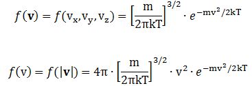
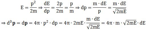
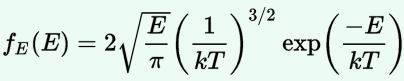
 Now, the final thing to note is that you’ll often want to use so-called normalized velocities, i.e. velocities that are defined as a v/v0 ratio, with v0 the most probable speed, which is equal to √(2kT/m). You get that value by calculating the df(v)/dv derivative, and then finding the value v = v0 for which df(v)/dv = 0. You should now be able to verify the formula that is used in the mentioned MIT version of the Stern-Gerlach experiment:
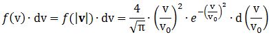 Indeed, when you write it all out – note that π/π3/2 = 1/√π 🙂 – you’ll see the two formulas are effectively equivalent. Of course, by now you are completely formula-ed out, and so you probably don’t even wonder what that f(v)·dv product actually stands for. What does it mean, really? Now you’ll sigh: why would I even want to know that? Well… I want you to understand
 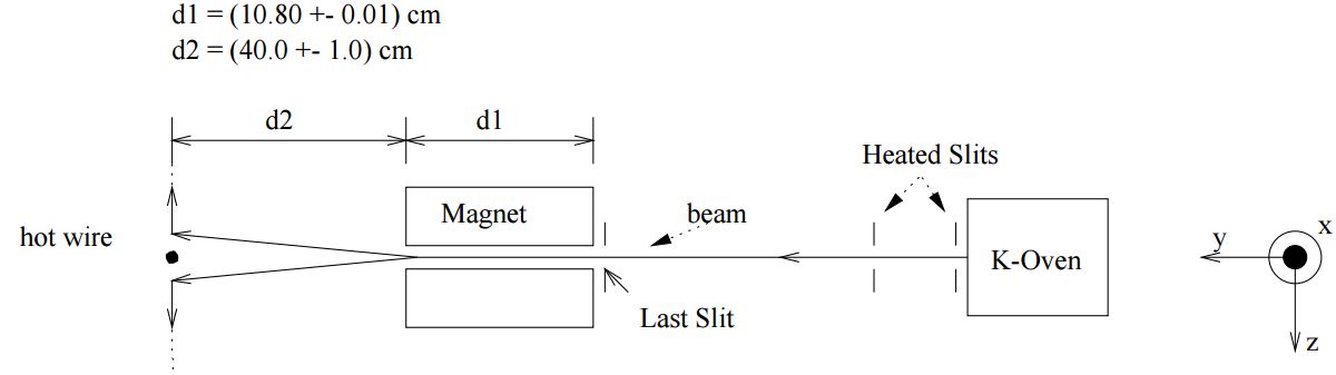 First, we’ll need some formula measuring the flux of (potassium) atoms coming out of the oven. And then… Well… Just have a look and try to make your way through
 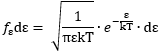 This holds true for any number of degrees of freedom. For example, a diatomic molecule will have extra degrees of freedom, which are related to its rotational and vibrational motion (I explained that in my June-July 2015 posts too, so please go there if you’d want to know more). So we can really use this stuff in, for example, the theory of the specific heat of gases. 🙂