Differential equations revisited: the math behind oscillators

Pre-scriptum (dated 26 June 2020): This post – part of a series of rather simple posts on elementary math and physics – does not seem to have been targeted in the the attack by the dark force—which is good because I still like it. While my views on the true nature of light, matter and the force or forces that act on them have evolved significantly as part of my explorations of a more realist (classical) explanation of quantum mechanics, I think most (if not all) of the analysis in this post remains valid and fun to read. In fact, I would dare to say the whole Universe consists of oscillators!

Original post:

When wrapping up my previous post, I said that I might be tempted to write something about how to solve these differential equations. The math behind them is pretty essential indeed. So let’s revisit the oscillator from a formal-mathematical point of view.

Modeling the problem

The simplest equation we used was the one for a hypothetical ‘ideal’ oscillator without friction and without any external driving force. The equation for a mechanical oscillator (i.e. a mass on a spring) is md²x/dt² = –kx. The k in this equation is a factor of proportionality: the force pulling back is assumed to be proportional to the amount of stretch, and the minus sign is there because the force is pulling back indeed. As for the equation itself, it’s just Newton’s Law: the mass times the acceleration equals the force: ma = F.

You’ll remember we preferred to write this as d²x/dt² = –(k/m)x = –ω₀²x with ω₀² = k/m. You’ll also remember that ω₀ is an angular frequency, which we referred to as the natural frequency of the oscillator (because it determines the natural motion of the spring indeed). We also gave the general solution to the differential equation: x(t) = x₀cos(ω₀t + Δ). That solution basically states that, if we just let go of that spring, it will oscillate with frequency ω₀ and some (maximum) amplitude x₀, the value of which depends on the initial conditions. As for the Δ term, that’s just a phase shift depending on where x is when we start counting time: if x would happen to pass through the equilibrium point at time t = 0, then Δ would be π/2. So Δ allows us to shift the beginning of time, so to speak.

In my previous posts, I just presented that general equation as a fait accompli, noting that a cosine (or sine) function does indeed have that ‘nice’ property of come back to itself with a minus sign in front after taking the derivative two times: d²[cos(ω₀t)]/dt² = –ω₀²cos(ω₀t). We could also write x(t) as a sine function because the sine and cosine function are basically the same except for a phase shift: x₀cos(ω₀t + Δ) = x₀sin(ω₀t + Δ + π/2).

Now, the point to note is that the sine or cosine function actually has two properties that are ‘nice’ (read ‘essential’ in the context of this discussion):

1. Sinusoidal functions are periodic functions and so that’s why they represent an oscillation–because that’s something periodic too!
2. Sinusoidal functions come back to themselves when we derive them two times and so that’s why it effectively solves our second-order differential equation.

However, in my previous post, I also mentioned in passing that sinusoidal functions share that second property with exponential functions: d²e^t/dt² = d[de^t/dt]/dt = de^t/dt = e^t. So, if it we would not have had that minus sign in our differential equation, our solution would have been some exponential function, instead of a sine or a cosine function. So what’s going on here?

Solving differential equations using exponentials

Let’s scrap that minus sign and assume our problem would indeed be to solve the d²x/dt² = ω₀²x equation. So we know we should use some exponential function, but we have that coefficient ω₀². Well… That’s actually easy to deal with: we know that, when deriving an exponential function, we should bring the exponent down as a coefficient: d[e^ω₀t]/dt = ω₀e^ω₀t. If we do it two times, we get d²[e^ω₀t]/dt² = ω₀²e^ω₀t, so we can immediately see that e^ω₀t is a solution indeed.

But it’s not the only one: e^–ω₀t is a solution too: d²[e^–ω₀t]/dt² = (–ω₀)(–ω₀)e^–ω₀t = ω₀²e^–ω₀t. So e^–ω₀t solves the equation too. It is easy to see why: ω₀² has two square roots–one positive, and one negative.

But we have more: in fact, every linear combination c₁e^ω₀t + c₂e^–ω₀t is also a solution to that second-order differential equation. Just check it by writing it all out: you’ll find that d²[c₁e^ω₀t + c₂e^–ω₀t]/dt² = ω₀²[c₁e^ω₀t +c₂e^–ω₀t] and so, yes, we have a whole family of functions here, that are all solutions to our differential equation.

Now, you may or may not remember that we had the same thing with first-order differential equations: we would find a whole family of functions, but only one would be the actual solution or the ‘real‘ solution I should say. So what’s the real solution here?

Well… That depends on the initial conditions: we need to know the value of x at time t₀ = 0 (or some other point t = t₁). And that’s not enough: we have two coefficients (c₁ and c₂), and, therefore, we need one more initial condition (it takes two equations to solve for two variables). That could be another value for x at some other point in time (e.g. t₂) but, when solving problems like this, you’ll usually get the other ‘initial condition’ expressed in terms of the first derivative, so that’s in terms of dx/dt = v. For example, it is not illogical to assume that the initial velocity v₀ would be zero. Indeed, we can imagine we pull or push the spring and then let it go. In fact, that’s what we’ve been assuming here all along in our example! Assuming that v₀ = 0 is equivalent to writing that

d[c₁e^ω₀t + c₂e^–ω₀t]/dt = 0 for t = 0

⇒ ω₀c₁ – ω₀c₂ = 0 (e⁰ = 1) ⇔  c₁ = c₂

Now we need the other initial condition. Let’s assume the initial value of x is equal to x₀ = 2 (it’s just an example: we could take any value, including negative values). Then we get:

c₁e^ω₀t + c₂e^–ω₀t = 2 for t = 0 ⇔ c₁ + c₂ = 2 (again, note that e⁰ = 1)

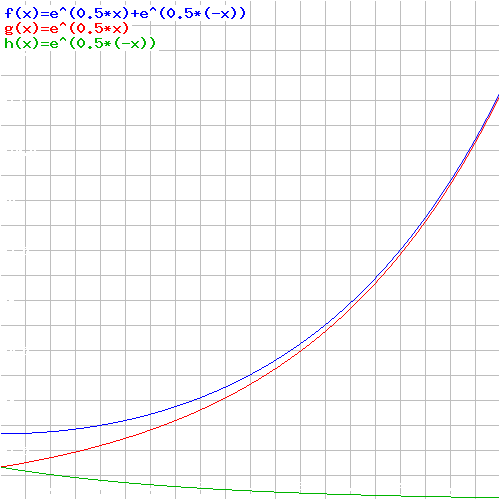
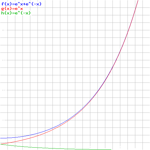
Combining the two gives us the grand result that c₁ = c₂ = 1 and, hence, the ‘real’ or actual solution is x = e^ω₀t + e^–ω₀t. The graph below plots that function for ω₀ = 1 and ω₀ = 0.5 respectively. We could take other values for ω₀ but, whatever the value, we’ll always get an exponential function like the ones below. It basically graphs what we expect to happen: the mass just accelerates away from its equilibrium point. Indeed, the differential equation is just a description of an accelerating object. Indeed, the e^–ω₀t term quickly goes to zero, and then it’s the e^ω₀t term that rockets that object sky-high – literally. [Note that the acceleration is actually not constant: the force is equal to kx and, hence, the force (and, therefore, the acceleration) actually increases as the mass goes further and further away from its equilibrium point. Also note that if the initial position would have been minus 2, i.e. x₀ = –2, then the object would accelerate away in the other direction, i.e. downwards. Just check it to make sure you understand the equations.]

The point to note is our general solution. More formally, and more generally, we get it as follows:

• If we have a linear second-order differential equation ax” + bx’ + cx = 0 (because of the zero on the right-hand side, we call such equation homogeneous, so it’s quite a mouthful: a linear and homogeneous DE of the second order), then we can find an exponential function e^rt that will be a solution for it.
• If such function is a solution, then plugging in it yields ar²e^rt + bre^rt + ce^rt = 0 or (ar² + br + c)e^rt = 0.
• Now, we can read that as a condition, and the condition amounts to ar² + br + c = 0. So that’s a quadratic equation we need to solve for r to find two specific solutions r₁ and r₂, which, in turn, will then yield our general solution:

 x(t) = c₁e^r₁t + c₂e^r₂t

Note that the general solution is based on the principle of superposition: any linear combination of two specific solutions will be a solution as well. I am mentioning this here because we’ll use that principle more than once.

Complex roots

The steps as described above implicitly assume that the quadratic equation above (i.e. ar²e^rt + bre^rt + ce^rt = 0), which is better known as the characteristic equation, does yield two real and distinct roots r₁ and r₂. In fact, it amounts to assuming that that exponential e^rt is a real-valued exponential function. We know how to find these real roots from our high school math classes: r = (–b ± [b² – 4ac]^1/2)/2a. However, what happens if the discrimant b² – 4ac is negative?

If the disciminant is negative, we will still have two roots, but they will be complex roots. In fact, we can write these two complex roots as r = α ± βi, with i the imaginary unit. Hence, the two complex roots are each other’s complex conjugate and our e^r₁t and e^r₂t can be written as:

e^r₁t = e^(α+βi)t and e^r₂t = e^(α–βi)t

Also, the general solution based on these two particular solutions will be c₁e^(α+βi)t + c₂e^(α–βi)t.

[You may wonder why complex roots have to be complex conjugates from each other. Indeed, that’s not so obvious from the raw r = (–b ± [b² – 4ac]^1/2)/2a formula. But you can re-write it as r = –b/2a ± [b² – 4ac]^1/2)/2a and, if b² – 4ac is negative, as r = –b/2a ± i·[(−b²+4ac)^1/2/2a]. So that gives you the α and β and shows that the two roots are, in effect, each other’s complex conjugate.]

We should briefly pause here to think about what we are doing here really: if we allow r to be complex, then what we’re doing really is allow a complex-valued function (to be precise: we’re talking the complex exponential functions e^(λ±μi)t, or any linear combination of the two) of a real variable (the time variable t) to be part of our ‘solution set’ as well.

Now, we’ve analyzed complex exponential functions before–long time ago: you can check out some of my posts last year (November 2013). In fact, we analyzed even more complex – in fact, I should say more complicated rather than more complex here: complex numbers don’t need to be complicated! 🙂 – because we were talking complex-valued functions of complex variables there! That’s not the case here: the argument t (i.e. the input into our function) is real, not complex, but the output – or the function itself – is complex-valued. Now, any complex exponential e^(α+βi)t can be written as e^αte^iβt, and so that’s easy enough to understand:

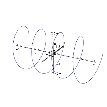
1. The first factor (i.e. e^αt) is just a real-valued exponential function and so we should be familiar with that. Depending on the value of α (negative or positive: see the graph below), it’s a factor that will create an envelope for our function. Indeed, when α is negative, the damping will cause the oscillation to stop after a while. When α is positive, we’ll have a solution resembling the second graph below: we have an amplitude that’s getting bigger and bigger, despite the friction factor (that’s obviously possible only because we keep reinforcing the movement, so we’re not switching off the force in that case). When α is equal to zero, then e^αt is equal to unity and so the amplitude will not change as the spring goes up and down over time: we have no friction in that case.

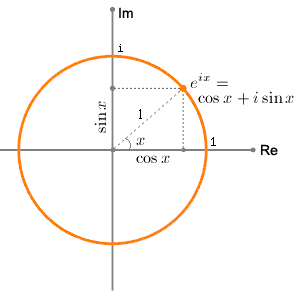
2. The second factor (i.e. e^iβt) is our periodic function. Indeed, e^iβt is the same as e^iθ and so just remember Euler’s formula to see what it is really:

e^iθ = cos(θ) + isin(θ)

The two graphs below represent the idea: as the phase θ = ωt + Δ (the angular frequency or velocity times the time is equal to the phase, plus or minus some phase shift) goes round and round and round (i.e. increases with time), the two components of e^iθ, i.e. the real and imaginary part e^iθ, oscillate between –1 and 1 because they are both sinusoidal functions (cosine and sine respectively). Now, we could amplify the amplitude by putting another (real) factor in front (a magnitude different than 1) and write re^iθ = r·cos(θ) + i·r·sin(θ) but that wouldn’t change the nature of this thing.

But so how does all of this relate to that other ‘general’ solution which we’ve found for our oscillator, i.e. the one we got without considering these complex-valued exponential functions as solutions. Indeed, what’s the relation between that x = x₀cos(ω₀t + Δ) equation and that rather frightening c₁e^(α+βi)t + c₂e^(α–βi)t equation? Perhaps we should look at x = x₀cos(ω₀t + Δ) as the real part of that monster? Yes and no. More no than yes actually. Actually… No. We are not going to have some complex exponential and then forget about the imaginary part. What we will do, though, is to find that general solution – i.e. a family of complex-valued functions – but then we’ll only consider those functions for which the imaginary part is zero, so that’s the subset of real-valued functions only.

I guess this must sound like Chinese. Let’s go step by step.

Using complex roots to find real-valued functions

If we re-write d²x/dt² = –ω₀²x in the more general ax” + bx’ + cx = 0 form, then we get x” + ω₀²x = 0 and so the discriminant b² – 4ac is equal to –4ω₀², and so that’s a negative number. So we need to go for these complex roots. However, before solving this, let’s first restate what we’re actually doing. We have a differential equation that, ultimately, depends on a real variable (the time variable t), but so now we allow complex-valued functions e^r₁t = e^(α+βi)t and e^r₂t = e^(α–βi)t as solutions. To be precise: these are complex-valued functions x of the real variable t.

That being said, it’s fine to note that real numbers are a subset of the complex numbers and so we can just shrug our shoulders and say all that we’re doing is switch to complex-valued functions because we got stuck with that negative determinant and so we had to allow for complex roots. However, in the end, we do want a real-valued solution x(t). So our x(t) = c₁e^(α+βi)t + c₂e^(α–βi)t has to be a real-valued function, not a complex-valued function.

That means that we have to take a subset of the family of functions that we’ve found. In other words, the imaginary part of  c₁e^(α+βi)t + c₂e^(α–βi)t has to be zero. How can it be zero? Well… It basically means that c₁e^(α+βi)t and c₂e^(α–βi)t have to be complex conjugates.

OK… But how do we do that? We need to find a way to write that c₁e^(α+βi)t + c₂e^(α–βi)t sum in a more manageable ζ + i·η form. We can do that by using Euler’s formula once again to re-write those two complex exponentials as follows:

• e^(α+βi)t = e^αte^iβt = e^αt[cos(βt) + isin(βt)]
• e^(α–βi)t = e^αte^–iβt = e^αt[cos(–βt) + isin(–βt)] = e^αt[cos(βt) – isin(βt)]

Note that, for the e^(α–βi)t expression, we’ve used the fact that cos(–θ) = cos(θ) and that sin(–θ) = –sin(θ). Also note that α and β are real numbers, so they do not have an imaginary part–unlike c₁ and c₂, which may or may not have an imaginary part (i.e. they could be pure real numbers, but they could be complex as well).

We can then re-write that c₁e^(α+βi)t + c₂e^(α–βi)t sum as:

c₁e^(α+βi)t + c₂e^(α–βi)t = c₁e^αt[cos(βt) + isin(βt)] + c₂e^αt[cos(βt) – isin(βt)]

= (c₁ + c₂)e^αtcos(βt) + (c₁ – c₂)ie^αtsin(βt)

So what? Well, we want that imaginary part in our solution to disappear and so it’s easy to see that the imaginary part will indeed disappear if c₁ – c₂ = 0, i.e. if c₁ = c₂ = c. So we have a fairly general real-valued solution x(t) = 2c·e^αtcos(βt) here, with c some real number. [Note that c has to be some real number because, if we would assume that c₁ and c₂ (and, therefore, c) would be equal complex numbers, then the c₁ – c₂ factor would also disappear, but then we would have a complex c₁ + c₂ sum in front of the e^αtcos(βt) factor, so that would defeat the purpose of finding real-valued function as a solution because (c₁ + c₂)e^αtcos(βt) would still be complex! […] Are you still with me? :-)]

So, OK, we’ve got the solution and so that should be it, isn’t it? Well… No. Wait. Not yet. Because these coefficients  c₁ and c₂ may be complex, there’s another solution as well. Look at that formula above. Let us suppose that c₁ would be equal to some (real) number c divided by i (so c₁ = c/i), and that c₂ would be its opposite, so c₂ = –c₁ (i.e. minus c₁). Then we would have two complex numbers consisting of an imaginary part only: c₁ = c/i and c₂ = –c₁ = –c/i, and they would be each other’s complex conjugate. Indeed, note that 1/i = i^–1= –i and so we can write c₁ = –c·i and c₂ = c·i. Then we’d get the following for that c₁e^(α+βi)t + c₂e^(α–βi)t sum:

 (c₁ + c₂)e^αtcos(βt) + (c₁ – c₂)ie^αtsin(βt)

= (c/i – c/i)e^αtcos(βt) + (c/i + c/i)ie^αtsin(βt) = 2c·e^αtsin(βt)

So, while c₁ and c₂ are complex, our grand result is a real-valued function once again or – to be precise – another family of real-valued functions (that’s because c can take on any value).

Are we done? Yes. There are no other possibilities. So now we just need to remember to apply the principle of superposition: any (real) linear combination of 2c·e^αtcos(μt) and 2c·e^αtsin(μt) will also be a (real-valued) solution, so the general (real-valued) solution for our problem is:

x(t) = a·2c·e^αtcos(βt) + b·2c·e^αtsin(βt) = Ae^αtcos(βt) + Be^αtsin(βt)

= e^αt[Acos(βt) + Bsin(βt)]

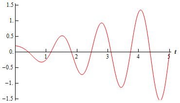
So what do we have here? Well, the first factor is, once again, an ‘envelope’ function: depending on the value of α, (i) negative, (ii) positive or (iii) zero, we have an oscillation that (i) damps out, (ii) goes out of control, or (iii) keeps oscillating in the same steady way forever.

The second part is equivalent to our ‘general’ x(t) = x₀cos(ω₀t + Δ) solution. Indeed, that x(t) = x₀cos(ω₀t + Δ) solution is somewhat less ‘general’ than the one above because it does not have the e^αt factor. However, x(t) = x₀cos(ω₀t + Δ) solution is equivalent to the Acos(βt) + Bsin(βt) factor. How’s that? We can show how they are related by using the trigonometric formula for adding angles: cos(α + β) = cos(α)cos(β) – sin(α)sin(β). Indeed, we can write:

x₀cos(ω₀t + Δ) = x₀cos(Δ)cos(ω₀t) – x₀sin(Δ)sin(ω₀t) = Acos(βt) + Bsin(βt)

with A = x₀cos(Δ), B = – x₀sin(Δ) and, finally, μ = ω₀

Are you convinced now? If not… Well… Nothing much I can do, I feel. In that case, I can only encourage you to do a full ‘work-out’ by reading the excellent overview of all possible situations in Paul’s Online MathNotes (tutorial.math.lamar.edu/Classes/DE/Vibrations.aspx).

Feynman’s treatment of second-order differential equations

Feynman takes a somewhat different approach in his Lectures. He solves them in a much more general way. At first, I thought his treatment was too confusing and, hence, I would not have mentioned it. However, I like the logic behind, even if his approach is somewhat more messy in terms of notations and all that. Let’s first look at the differential equation once again. Let’s take a system with a friction factor that’s proportional to the speed: F_f = –c·dx/dt. [See my previous post for some comments on that assumption: the assumption is, generally speaking, too much of a simplification but it makes for a ‘nice’ linear equation and so that’s why physicists present it that way.] To ease the math, c is usually written as c = mγ. Hence, γ = c/m is the friction per unit of mass. That makes sense, I’d think. In addition, we need to remember that ω₀² = k/m, so k = mω₀². Our differential equation then becomes m·d²x/dt² = –γm·dx/dt – kx (mass times acceleration is the sum of the forces) or m·d²x/dt² + γm·dx/dt + mω₀²·x = 0. Dividing the mass factor away gives us an even simpler form:

d²x/dt² + γdx/dt + ω₀²x = 0

You’ll remember this differential equation from the previous post: we used it to calculate the (stored) energy and the Q of a mechanical oscillator. However, we didn’t show you how. You now understand why: the stuff above is not easy–the length of the arguments involved is why I am devoting an entire post to it!

Now, instead of assuming some exponential e^rt as a solution, real- or complex-valued, Feynman assumes a much more general complex-valued function as solution: he substitutes x for x = Ae^iαt, with A a complex number as well so we can write A as A = A₀e^iΔ. That more general assumption allows for the inclusion of a phase shift straight from the start. Indeed, we can write x as x = A₀e^iΔe^iαt = = A₀e^i(αt+Δ). Does that look complicated? It probably does, because we also have to remember that α is a complex number! So we’ve got a very general complex-valued exponential function indeed here!

However, let’s not get ahead of ourselves and follow Feynman. So he plugs in that complex-valued x = Ae^iαt and we get:

(–α² + iγα + ω₀²)Ae^iαt = 0

So far, so good. The logic now is more or less the same as the logic we developed above. We’ve got two factors here: (1) a quadratic equation –α² + iγα + ω₀² (with one complex coefficient iγ) and (2) a complex exponential function Ae^iαt. The second factor (Ae^iαt) cannot be zero, because that’s x and we assume our oscillator is not standing still. So it’s the first factor (i.e. the quadratic equation in α with a complex coefficient iγ) which has to be zero. So we solve for the roots α and find

α = –iγ/(–2) ± i·[(–(iγ)²–4ω₀²)^1/2/(-2)] = iγ/2 ± i·[(γ²–4ω₀²)^1/2/(-2)]

= iγ/2 ± (ω₀² – γ²/4)^1/2 = iγ/2 ± ω_γ

[We get this by bringing i and –2 inside of the square root expression. It’s not very straightforward but you should be able to figure it out.]

So that’s an interesting expression: the imaginary part of α is iγ/2 and its real part is (ω₀² – γ²/4)^1/2, which we denoted as ω_γ in the expression above. [Note that we assume there’s no problem with the square root expression: γ²/4 should be smaller than ω₀² so ω_γ is supposed to be some real positive number.] And so we’ve got the two solutions x₁ and x₂:

x₁ = Ae^{i(iγ/2 + ω_γ)t} =  Ae^{–γt/2+iω_γt} = Ae^–γt/2e^iω_γt 

x₂ = Be^{i(iγ/2 – ω_γ)t} =  Be^{–γt/2–iω_γt} = Be^–γt/2e^–iω_γt

Note, once again, that A and B can be any (complex) number and that, because of the principle of superposition, any linear combination of these two solutions will also be a solution. So the general solution is

x = Ae^–γt/2e^iω_γt + Be^–γt/2e^–iω_γt = e^–γt/2(Ae^iω_γt + Be^–iω_γt) 

Now, we recognize the shape of this: a (real-valued) envelope function e^–γt/2 and then a linear combination of two exponentials. But so we want something real-valued in the end so, once again, we need to impose the condition that Ae^iω_γt and Be^–iω_γt are complex conjugates of each other. Now, we can see that e^iω_γt and e^–iω_γt are complex conjugates but what does this say about A and B? Well… The complex conjugate of a product is the product of the complex conjugates of the factors involved: (z₁z₂)* = (z₁*)(z₁*). That implies that B has to be the complex conjugate of A: B = A*. So the final (real-valued) solution becomes:

x = e^–γt/2(Ae^iω_γt + A*e^–iω_γt) 

Now, I’ll leave it to you to prove that the second factor in the product above (Ae^iω_γt + A*e^–iω_γt) is a real-valued function of the real variable t. It should be the same as x₀cos(Δ)cos(ω₀t) – x₀sin(Δ)sin(ω₀t), and that gives you a graph like the one below. However, I can readily imagine that, by now, you’re just thinking: Oh well… Whatever! 🙂

So the difference between Feynman’s approach and the one I presented above (which is the one you’ll find in most textbooks) is the assumption in terms of the specific solution: instead of substituting x for e^rt, with allowing r to take on complex values, Feynman substitutes x for Ae^iαt, and allows both A and α  to take on complex values. It makes the calculations more complicated but, when everything is said and done, I think Feynman’s approach is more consistent because more encompassing. However, that’s subject to taste, and I gather, from comments on the Web, that many people think that this chapter in Feynman’s Lectures is not his best. So… Well… I’ll leave it to you to make the final judgment.

Note: The one critique that is relevant, in regard to Feynman’s treatment of the matter, is that he devotes quite a bit of time and space to explain how these oscillatory or periodic displacements can be viewed as being the real part of a complex exponential. Indeed, cos(ωt) is the real part of e^iωt. But so that’s something different than (1) expanding the realm of possible solutions to a second-order differential equation from real-valued functions to complex-valued functions in order to (2) then, once we’ve found the general solution, consider only real-valued functions once again as ‘allowable’ solutions to that equation. I think that’s the gist of the matter really. It took me a while to fully ‘get’ this. I hope this post helps you to understand it somewhat quicker than I did. 🙂

Conclusion

I guess the only thing that I should do now is to work some examples. However, I’ll refer you Paul’s Online Math Notes for that once again (see the reference above). Indeed, it is about time I end my rather lengthy exposé (three posts on the same topic!) on oscillators and resonance. I hope you enjoyed it, although I can readily imagine that it’s hard to appreciate the math involved.

It is not easy indeed: I actually struggled with it, despite the fact that I think I understand complex analysis somewhat. However, the good thing is that, once we’re through it, we can really solve a lot of problems. As Feynman notes: “Linear (differential) equations are so important that perhaps fifty percent of the time we are solving linear equations in physics and engineering.” So, bearing in that mind, we should move on to the next.

Some content on this page was disabled on June 16, 2020 as a result of a DMCA takedown notice from The California Institute of Technology. You can learn more about the DMCA here:

https://en.support.wordpress.com/copyright-and-the-dmca/