The photon wavefunction

Post scriptum note added on 11 July 2016: This is one of the more speculative posts which led to my e-publication analyzing the wavefunction as an energy propagation. With the benefit of hindsight, I would recommend you to immediately the more recent exposé on the matter that is being presented here, which you can find by clicking on the provided link.

Original post:

In my previous posts, I juxtaposed the following images:

Both are the same, and then they’re not. The illustration on the left-hand side shows how the electric field vector (E) of an electromagnetic wave travels through space, but it does not show the accompanying magnetic field vector (B), which is as essential in the electromagnetic propagation mechanism according to Maxwell’s equations:

∂B/∂t = –∇×E
∂E/∂t = c²∇×B = ∇×B for c = 1

The second illustration shows a wavefunction eⁱ^{(kx − ωt)}= cos(kx − ωt) + i∙sin(kx − ωt). Its propagation mechanism—if we can call it like that—is Schrödinger’s equation:

∂ψ/∂t = i·(ħ/2m)·∇²ψ

We already drew attention to the fact that an equation like this models some flow. To be precise, the Laplacian on the right-hand side is the second derivative with respect to x here, and, therefore, expresses a flux density: a flow per unit surface area, i.e. per square meter. To be precise: the Laplacian represents the flux density of the gradient flow of ψ.

On the left-hand side of Schrödinger’s equation, we have a time derivative, so that’s a flow per second. The ħ/2m factor is like a diffusion constant. In fact, strictly speaking, that ħ/2m factor is a diffusion constant, because it does exactly the same thing as the diffusion constant D in the diffusion equation ∂φ/∂t = D·∇²φ, i.e:

As a constant of proportionality, it quantifies the relationship between both derivatives.
As a physical constant, it ensures the dimensions on both sides of the equation are compatible.

So our diffusion constant here is ħ/2m. Because of the Uncertainty Principle, m is always going to be some integer multiple of ħ/2, so ħ/2m = 1, 1/2, 1/3, 1/4 etcetera. In other words, the ħ/2m term is the inverse of the mass measured in units of ħ/2. We get the terms of the harmonic series here. How convenient! 🙂

In our previous posts, we studied the wavefunction for a zero-mass particle. Such particle has zero rest mass but – because of its movement – does have some energy, and, therefore, some mass and momentum. In fact, measuring time and distance in equivalent units (so c = 1), we found that E = m = p = ħ/2 for the zero-mass particle. It had to be. If not, our equations gave us nonsense. So Schrödinger’s equation was reduced to:

∂ψ/∂t = i·∇²ψ

How elegant! We only need to explain that imaginary unit (i) in the equation. It does a lot of things. First, it gives us two equations for the price of one—thereby providing a propagation mechanism indeed. It’s just like the E and B vectors. Indeed, we can write that ∂ψ/∂t = i·∇²ψ equation as:

Re(∂ψ/∂t) = −Im(∇²ψ)
Im(∂ψ/∂t) = Re(∇²ψ)

You should be able to show that the two equations above are effectively equivalent to Schrödinger’s equation. If not… Well… Then you should not be reading this stuff.] The two equations above show that the real part of the wavefunction feeds into its imaginary part, and vice versa. Both are as essential. Let me say this one more time: the so-called real and imaginary part of a wavefunction are equally real—or essential, I should say!

Second, i gives us the circle. Huh? Yes. Writing the wavefunction as ψ = a + i·b is not just like writing a vector in terms of its Cartesian coordinates, even if it looks very much that way. Why not? Well… Never forget: i²= −1, and so—let me use mathematical lingo here—the introduction of i makes our metric space complete. To put it simply: we can now compute everything. In short, the introduction of the imaginary unit gives us that wonderful mathematical construct, eⁱ^{(kx − ωt)}, which allows us to model everything. In case you wonder, I mean: everything! Literally. 🙂

However, we’re not going to impose any pre-conditions here, and so we’re not going to make that E = m = p = ħ/2 assumption now. We’ll just re-write Schrödinger’s equation as we did last time—so we’re going to keep our ‘diffusion constant’ ħ/2m as for now:

Re(∂ψ/∂t) = −(ħ/2m)·Im(∇²ψ)
Im(∂ψ/∂t) = (ħ/2m)·Re(∇²ψ)

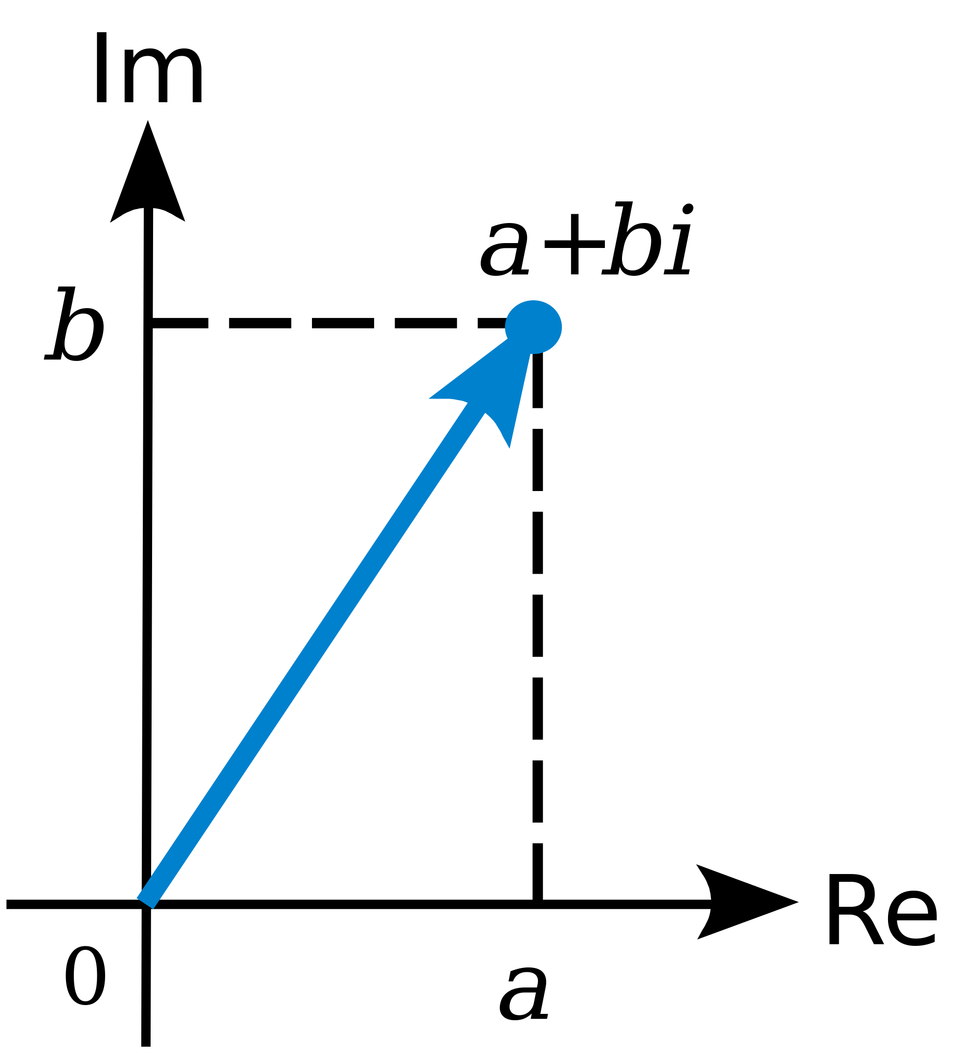
So we have two pairs of equations now. Can they be related? Well… They look the same, so they had better be related! 🙂 Let’s explore it. First note that, if we’d equate the direction of propagation with the x-axis, we can write the E vector as the sum of two y- and z-components: E = (E_y, E_z). Using complex number notation, we can write E as:

E = (E_y, E_z) = E_y + i·E_z

In case you’d doubt, just think of this simple drawing:

The next step is to imagine—funny word when talking complex numbers—that E_y and E_zare the real and imaginary part of some wavefunction, which we’ll denote as ψ_E = eⁱ^{(kx − ωt)}. So now we can write:

E = (E_y, E_z) = E_y + i·E_z= cos(kx − ωt) + i∙sin(kx − ωt) = Re(ψ_E) + i·Im(ψ_E)

What’s k and ω? Don’t worry about it—for the moment, that is. We’ve done nothing special here. In fact, we’re used to representing waves as some sine or cosine function, so that’s what we are doing here. Nothing more. Nothing less. We just need two sinusoids because of the circular polarization of our electromagnetic wave.

What’s next? Well… If ψ_E is a regular wavefunction, then we should be able to check if it’s a solution to Schrödinger’s equation. So we should be able to write:

Re(∂ψ_E/∂t) = −(ħ/2m)·Im(∇²ψ_E)
Im(∂ψ_E/∂t) = (ħ/2m)·Re(∇²ψ_E)

Are we? How does that work? The time derivative on the left-hand side is equal to:

∂ψ_E/∂t = −iω·eⁱ^{(kx − ωt)}= −iω·[cos(kx − ωt) + i·sin(kx − ωt)] = ω·sin(kx − ωt) − iω·cos(kx − ωt)

The second-order derivative on the right-hand side is equal to:

∇²ψ_E= ∂²ψ_E/∂x²= −k²·eⁱ^{(kx − ωt)}= −k²·cos(kx − ωt) − ik²·sin(kx − ωt)

So the two equations above are equivalent to writing:

Re(∂ψ_E/∂t) = −(ħ/2m)·Im(∇²ψ_E) ⇔ ω·sin(kx − ωt) = k²·(ħ/2m)·sin(kx − ωt)
Im(∂ψ_E/∂t) = (ħ/2m)·Re(∇²ψ_E) ⇔ −ω·cos(kx − ωt) = −k²·(ħ/2m)·cos(kx − ωt)

Both conditions are fulfilled if, and only if, ω = k²·(ħ/2m). Now, assuming we measure time and distance in equivalent units (c = 1), we can calculate the phase velocity of the electromagnetic wave as being equal to c = ω/k = 1. We also have the de Broglie equation for the matter-wave, even if we’re not quite sure whether or not we should apply that to an electromagnetic wave. In any case, the de Broglie equation tells us that k = p/ħ. So we can re-write this condition as:

ω/k = 1 = k·(ħ/2m) = (p/ħ)·(ħ/2m) = p/2m ⇔ p = 2m ⇔ m = p/2

So that’s different from the E = m = p equality we imposed when discussing the wavefunction of the zero-mass particle: we’ve got that 1/2 factor which bothered us so much once again! And it’s causing us the same trouble: how do we interpret that m = p/2 equation? It leads to nonsense once more! E = m·c²= m, but E is also supposed to be equal to p·c = p. Here, however, we find that E = p/2! We also get strange results when calculating the group and phase velocity. So… Well… What’s going on here?

I am not quite sure. It’s that damn 1/2 factor. Perhaps it’s got something to do with our definition of mass. The m in the Schrödinger equation was referred to as the effective or reduced mass of the electron wavefunction that it was supposed to model. Now that concept is something funny: it sure allows for some gymnastics, as you’ll see when going through the Wikipedia article on it! I promise I’ll dig into it—but not now and here, as I’ve got no time for that. 😦

However, the good news is that we also get a magnetic field vector with an electromagnetic wave: B. We know B is always orthogonal to E, and in the direction that’s given by the right-hand rule for the vector cross-product. Indeed, we can write B as B = e_x×E/c, with e_x the unit vector pointing in the x-direction (i.e. the direction of propagation), as shown below.

E and b

So we can do the same analysis: we just substitute E for B everywhere, and we’ll find the same condition: m = p/2. To distinguish the two wavefunctions, we used the E and B subscripts for our wavefunctions, so we wrote ψ_Eand ψ_B. We can do the same for that m = p/2 condition:

m_E= p_E/2
m_B= p_B/2

Should we just add m_Eand m_E to get a total momentum and, hence, a total energy, that’s equal to E = m = p for the whole wave? I believe we should, but I haven’t quite figured out how we should interpret that summation!

So… Well… Sorry to disappoint you. I haven’t got the answer here. But I do believe my instinct tells me the truth: the wavefunction for an electromagnetic wave—so that’s the wavefunction for a photon, basically—is essentially the same as our wavefunction for a zero-mass particle. It’s just that we get two wavefunctions for the price of one. That’s what distinguishes bosons from fermions! And so I need to figure out how they differ exactly! And… Well… Yes. That might take me a while!

In the meanwhile, we should play some more with those E and B vectors, as that’s going to help us to solve the riddle—no doubt!

Fiddling with E and B

The B = e_x×E/c equation is equivalent to saying that we’ll get B when rotating E by 90 degrees which, in turn, is equivalent to multiplication by the imaginary unit i. Huh? Yes. Sorry. Just google the meaning of the vector cross product and multiplication by i. So we can write B = i·E, which amounts to writing:

B = i·E = eⁱ^(π/2)·eⁱ^{(kx − ωt)} = eⁱ^{(kx − ωt + π/2)} = cos(kx − ωt + π/2) + i·sin(kx − ωt + π/2)

So we can now associate a wavefunction ψ_B with the field magnetic field vector B, which is the same wavefunction as ψ_E except for a phase shift equal to π/2. You’ll say: so what? Well… Nothing much. I guess this observation just concludes this long digression on the wavefunction of a photon: it’s the same wavefunction as that of a zero-mass particle—except that we get two for the price of one!

It’s an interesting way of looking at things. Let’s look at the equations we started this post with, i.e. Maxwell’s equations in free space—i.e. no stationary charges, and no currents (i.e. moving charges) either! So we’re talking those ∂B/∂t = –∇×E and ∂E/∂t = ∇×B equations now.

Note that they actually give you four equations, because they’re vector equations:

∂B/∂t = –∇×E ⇔ ∂B_y/∂t = –(∇×E)_y and ∂B_z/∂t = –(∇×E)_z
∂E/∂t = ∇×B ⇔ ∂E_y/∂t = (∇×B)_y and ∂E_z/∂t = (∇×B)_z

To figure out what that means, we need to remind ourselves of the definition of the curl operator, i.e. the ∇× operator. For E, the components of ∇×E are the following:

(∇×E)_z = ∇_xE_y– ∇_yE_x= ∂E_y/∂x – ∂E_x/∂y
(∇×E)_x = ∇_yE_z– ∇_zE_y= ∂E_z/∂y – ∂E_y/∂z
(∇×E)_y = ∇_zE_x– ∇_xE_z= ∂E_x/∂z – ∂E_z/∂x

So the four equations above can now be written as:

∂B_y/∂t = –(∇×E)_y = –∂E_x/∂z + ∂E_z/∂x
∂B_z/∂t = –(∇×E)_z = –∂E_y/∂x + ∂E_x/∂y
∂E_y/∂t = (∇×B)_y = ∂B_x/∂z – ∂B_z/∂x
∂E_z/∂t = (∇×B)_z= ∂B_y/∂x – ∂B_x/∂y

What can we do with this? Well… The x-component of E and B is zero, so one of the two terms in the equations simply disappears. We get:

∂B_y/∂t = –(∇×E)_y = ∂E_z/∂x
∂B_z/∂t = –(∇×E)_z = – ∂E_y/∂x
∂E_y/∂t = (∇×B)_y = – ∂B_z/∂x
∂E_z/∂t = (∇×B)_z= ∂B_y/∂x

Interesting: only the derivatives with respect to x remain! Let’s calculate them:

∂B_y/∂t = –(∇×E)_y = ∂E_z/∂x = ∂[sin(kx − ωt)]/∂x = k·cos(kx − ωt) = k·E_y
∂B_z/∂t = –(∇×E)_z = – ∂E_y/∂x = – ∂[cos(kx − ωt)]/∂x = k·sin(kx − ωt) = k·E_z
∂E_y/∂t = (∇×B)_y = – ∂B_z/∂x = – ∂[sin(kx − ωt + π/2)]/∂x = – k·cos(kx − ωt + π/2) = – k·B_y
∂E_z/∂t = (∇×B)_z= ∂B_y/∂x = ∂[cos(kx − ωt + π/2)]/∂x = − k·sin(kx − ωt + π/2) = – k·B_z

What wonderful results! The time derivatives of the components of B and E are equal to ±k times the components of E and B respectively! So everything is related to everything, indeed! 🙂

Let’s play some more. Using the cos(θ + π/2) = −sin(θ) and sin(θ + π/2) = cos(θ) identities, we know that B_y and B_z= sin(kx − ωt + π/2) are equal to:

B_y= cos(kx − ωt + π/2) = −sin(kx − ωt) = −E_z
B_z= sin(kx − ωt + π/2) = cos(kx − ωt) = E_y

Let’s calculate those derivatives once more now:

∂B_y/∂t = −∂E_z/∂t = −∂sin(kx − ωt)/∂t = ω·cos(kx − ωt) = ω·E_y
∂B_z/∂t = ∂E_y/∂t = ∂cos(kx − ωt)/∂t = −ω·sin(kx − ωt) = −ω·E_z

This result can, obviously, be true only if ω = k, which we assume to be the case, as we’re measuring time and distance in equivalent units, so the phase velocity is c = 1 = ω/k.

Hmm… I am sure it won’t be long before I’ll be able to prove what I want to prove. I just need to figure out the math. It’s pretty obvious now that the wavefunction—any wavefunction, really—models the flow of energy. I just need to show how it works for the zero-mass particle—and then I mean: how it works exactly. We must be able to apply the concept of the Poynting vector to wavefunctions. We must be. I’ll find how. One day. 🙂

As for now, however, I feel we’ve played enough with those wavefunctions now. It’s time to do what we promised to do a long time ago, and that is to use Schrödinger’s equation to calculate electron orbitals—and other stuff, of course! Like… Well… We hardly ever talked about spin, did we? That comes with huge complexities. But we’ll get through it. Trust me. 🙂

The wavefunction of a zero-mass particle

Original post:

I hope you find the title intriguing. A zero-mass particle? So I am talking a photon, right? Well… Yes and no. Just read this post and, more importantly, think about this story for yourself. 🙂

One of my acquaintances is a retired nuclear physicist. We mail every now and then—but he has little or no time for my questions: he usually just tells me to keep studying. I once asked him why there is never any mention of the wavefunction of a photon in physics textbooks. He bluntly told me photons don’t have a wavefunction—not in the sense I was talking at least. Photons are associated with a traveling electric and a magnetic field vector. That’s it. Full stop. Photons do not have a ψ or φ function. [I am using ψ and φ to refer to position or momentum wavefunction. You know both are related: if we have one, we have the other.] But then I never give up, of course. I just can’t let go out of the idea of a photon wavefunction. The structural similarity in the propagation mechanism of the electric and magnetic field vectors E and B just looks too much like the quantum-mechanical wavefunction. So I kept trying and, while I don’t think I fully solved the riddle, I feel I understand it much better now. Let me show you the why and how.

I. An electromagnetic wave in free space is fully described by the following two equations:

∂B/∂t = –∇×E
∂E/∂t = c²∇×B

We’re making abstraction here of stationary charges, and we also do not consider any currents here, so no moving charges either. So I am omitting the ∇·E = ρ/ε₀ equation (i.e. the first of the set of four equations), and I am also omitting the j/ε₀ in the second equation. So, for all practical purposes (i.e. for the purpose of this discussion), you should think of a space with no charges: ρ = 0 and j = 0. It’s just a traveling electromagnetic wave. To make things even simpler, we’ll assume our time and distance units are chosen such that c = 1, so the equations above reduce to:

∂B/∂t = –∇×E
∂E/∂t = ∇×B

Perfectly symmetrical! But note the minus sign in the first equation. As for the interpretation, I should refer you to previous posts but, briefly, the ∇× operator is the curl operator. It’s a vector operator: it describes the (infinitesimal) rotation of a (three-dimensional) vector field. We discussed heat flow a couple of times, or the flow of a moving liquid. So… Well… If the vector field represents the flow velocity of a moving fluid, then the curl is the circulation density of the fluid. The direction of the curl vector is the axis of rotation as determined by the ubiquitous right-hand rule, and its magnitude of the curl is the magnitude of rotation. OK. Next step.

II. For the wavefunction, we have Schrödinger’s equation, ∂ψ/∂t = i·(ħ/2m)·∇²ψ, which relates two complex-valued functions (∂ψ/∂t and ∇²ψ). Complex-valued functions consist of a real and an imaginary part, and you should be able to verify this equation is equivalent to the following set of two equations:

Re(∂ψ/∂t) = −(ħ/2m)·Im(∇²ψ)
Im(∂ψ/∂t) = (ħ/2m)·Re(∇²ψ)

[Two complex numbers a + ib and c + id are equal if, and only if, their real and imaginary parts are the same. However, note the −i factor in the right-hand side of the equation, so we get: a + ib = −i·(c + id) = d −ic.] The Schrödinger equation above also assumes free space (i.e. zero potential energy: V = 0) but, in addition – see my previous post – they also assume a zero rest mass of the elementary particle (E₀ = 0). So just assume E₀= V = 0 in de Broglie’s elementary ψ(θ) = ψ(x, t) = e⁻ⁱ^θ = a·e^{−i[(E₀+ p2/(2m) + V)·t − p∙x]/ħ} wavefunction. So, in essence, we’re looking at the wavefunction of a massless particle here. Sounds like nonsense, doesn’t it? But… Well… That should be the wavefunction of a photon in free space then, right? 🙂

Maybe. Maybe not. Let’s go as far as we can.

The energy of a zero-mass particle

What m would we use for a photon? It’s rest mass is zero, but it’s got energy and, hence, an equivalent mass. That mass is given by the m = E/c²mass-energy equivalence. We also know a photon has momentum, and it’s equal to its energy divided by c: p = m·c = E/c. [I know the notation is somewhat confusing: E is, obviously, not the magnitude of E here: it’s energy!] Both yield the same result. We get: m·c = E/c ⇔ m = E/c²⇔ E = m·c².

OK. Next step. Well… I’ve always been intrigued by the fact that the kinetic energy of a photon, using the E = m·v²/2 = E = m·c²/2 formula, is only half of its total energy E = m·c². Half: 1/2. That 1/2 factor is intriguing. Where’s the rest of the energy? It’s really a contradiction: our photon has no rest mass, and there’s no potential here, but its total energy is still twice its kinetic energy. Quid?

There’s only one conclusion: just because of its sheer existence, it must have some hidden energy, and that hidden energy is also equal to E = m·c²/2, and so the kinetic and hidden energy add up to E = m·c².

Huh? Hidden energy? I must be joking, right?

Well… No. No joke. I am tempted to call it the imaginary energy, because it’s linked to the imaginary part of the wavefunction—but then it’s everything but imaginary: it’s as real as the imaginary part of the wavefunction. [I know that sounds a bit nonsensical, but… Well… Think about it: it does make sense.]

Back to that factor 1/2. You may or may not remember it popped up when we were calculating the group and the phase velocity of the wavefunction respectively, again assuming zero rest mass, and zero potential. [Note that the rest mass term is mathematically equivalent to the potential term in both the wavefunction as well as in Schrödinger’s equation: (E₀·t +V·t = (E₀+ V)·t, and V·ψ + E₀·ψ = (V+E₀)·ψ—obviously!]

In fact, let me quickly show you that calculation again: the de Broglie relations tell us that the k and the ω in the eⁱ^{(kx − ωt)} = cos(kx−ωt) + i∙sin(kx−ωt) wavefunction (i.e. the spatial and temporal frequency respectively) are equal to k = p/ħ, and ω = E/ħ. If we would now use the kinetic energy formula E = m·v²/2 – which we can also write as E = m·v·v/2 = p·v/2 = p·p/2m = p²/2m, with v = p/m the classical velocity of the elementary particle that Louis de Broglie was thinking of – then we can calculate the group velocity of our eⁱ^{(kx − ωt)} = cos(kx−ωt) + i∙sin(kx−ωt) as:

v_g = ∂ω/∂k = ∂[E/ħ]/∂[p/ħ] = ∂E/∂p = ∂[p²/2m]/∂p = 2p/2m = p/m = v

[Don’t tell me I can’t treat m as a constant when calculating ∂ω/∂k: I can. Think about it.] Now the phase velocity. The phase velocity of our eⁱ^{(kx − ωt)} is only half of that. Again, we get that 1/2 factor:

v_p = ω/k = (E/ħ)/(p/ħ) = E/p = (p²/2m)/p = p/2m = v/2

Strange, isn’t it? Why would we get a different value for the phase velocity here? It’s not like we have two different frequencies here, do we? You may also note that the phase velocity turns out to be smaller than the group velocity, which is quite exceptional as well! So what’s the matter?

Well… The answer is: we do seem to have two frequencies here while, at the same time, it’s just one wave. There is only one k and ω here but, as I mentioned a couple of times already, that eⁱ^{(kx − ωt)} wavefunction seems to give you two functions for the price of one—one real and one imaginary: eⁱ^{(kx − ωt)} = cos(kx−ωt) + i∙sin(kx−ωt). So are we adding waves, or are we not? It’s a deep question. In my previous post, I said we were adding separate waves, but now I am thinking: no. We’re not. That sine and cosine are part of one and the same whole. Indeed, the apparent contradiction (i.e. the different group and phase velocity) gets solved if we’d use the E = m∙v² formula rather than the kinetic energy E = m∙v²/2. Indeed, assuming that E = m∙v² formula also applies to our zero-mass particle (I mean zero rest mass, of course), and measuring time and distance in natural units (so c = 1), we have:

E = m∙c² = m and p = m∙c²= m, so we get: E = m = p

Waw! What a weird combination, isn’t it? But… Well… It’s OK. [You tell me why it wouldn’t be OK. It’s true we’re glossing over the dimensions here, but natural units are natural units, and so c = c²= 1. So… Well… No worries!] The point is: that E = m = p equality yields extremely simple but also very sensible results. For the group velocity of our eⁱ^{(kx − ωt)} wavefunction, we get:

v_g = ∂ω/∂k = ∂[E/ħ]/∂[p/ħ] = ∂E/∂p = ∂p/∂p = 1

So that’s the velocity of our zero-mass particle (c, i.e. the speed of light) expressed in natural units once more—just like what we found before. For the phase velocity, we get:

v_p = ω/k = (E/ħ)/(p/ħ) = E/p = p/p = 1

Same result! No factor 1/2 here! Isn’t that great? My ‘hidden energy theory’ makes a lot of sense. 🙂 In fact, I had mentioned a couple of times already that the E = m∙v² relation comes out of the de Broglie relations if we just multiply the two and use the v = f·λ relation:

f·λ = (E/h)·(h/p) = E/p
v = f·λ ⇒ f·λ = v = E/p ⇔ E = v·p = v·(m·v) ⇒ E = m·v²

But so I had no good explanation for this. I have one now: the E = m·v²is the correct energy formula for our zero-mass particle. 🙂

The quantization of energy and the zero-mass particle

Let’s now think about the quantization of energy. What’s the smallest value for E that we could possible think of? That’s h, isn’t it? That’s the energy of one cycle of an oscillation according to the Planck-Einstein relation (E = h·f). Well… Perhaps it’s ħ? Because… Well… We saw energy levels were separated by ħ, rather than h, when studying the blackbody radiation problem. So is it ħ = h/2π? Is the natural unit a radian (i.e. a unit distance), rather than a cycle?

Neither is natural, I’d say. We also have the Uncertainty Principle, which suggests the smallest possible energy value is ħ/2, because ΔxΔp = ΔtΔE = ħ/2.

Huh? What’s the logic here?

Well… I am not quite sure but my intuition tells me the quantum of energy must be related to the quantum of time, and the quantum of distance.

Huh? The quantum of time? The quantum of distance? What’s that? The Planck scale?

No. Or… Well… Let me correct that: not necessarily. I am just thinking in terms of logical concepts here. Logically, as we think of the smallest of smallest, then our time and distance variables must become count variables, so they can only take on some integer value n = 0, 1, 2 etcetera. So then we’re literally counting in time and/or distance units. So Δx and Δt are then equal to 1. Hence, Δp and ΔE are then equal to Δp = ΔE = ħ/2. Just think of the radian (i.e. the unit in which we measure θ) as measuring both time as well as distance. Makes sense, no?

No? Well… Sorry. I need to move on. So the smallest possible value for m = E = p would be ħ/2. Let’s substitute that in Schrödinger’s equation, or in that set of equations Re(∂ψ/∂t) = −(ħ/2m)·Im(∇²ψ) and Im(∂ψ/∂t) = (ħ/2m)·Re(∇²ψ). We get:

Re(∂ψ/∂t) = −(ħ/2m)·Im(∇²ψ) = −(2ħ/2ħ)·Im(∇²ψ) = −Im(∇²ψ)
Im(∂ψ/∂t) = (ħ/2m)·Re(∇²ψ) = (2ħ/2ħ)·Re(∇²ψ) = Re(∇²ψ)

Bingo! The Re(∂ψ/∂t) = −Im(∇²ψ) and Im(∂ψ/∂t) = Re(∇²ψ) equations were what I was looking for. Indeed, I wanted to find something that was structurally similar to the ∂B/∂t = –∇×E and ∂E/∂t = ∇×B equations—and something that was exactly similar: no coefficients in front or anything. 🙂

What about our wavefunction? Using the de Broglie relations once more (k = p/ħ, and ω = E/ħ), our eⁱ^{(kx − ωt)} = cos(kx−ωt) + i∙sin(kx−ωt) now becomes:

eⁱ^{(kx − ωt)} = eⁱ^{(ħ·x/2 − ħ·t/2)/ħ} = eⁱ^{(x/2 − t/2)}= cos[(x−t)/2] + i∙sin[(x−t)/2]

Hmm… Interesting! So we’ve got that 1/2 factor now in the argument of our wavefunction! I really feel I am close to squaring the circle here. 🙂 Indeed, it must be possible to relate the ∂B/∂t = –∇×E and ∂E/∂t = c²∇×B to the Re(∂ψ/∂t) = −Im(∇²ψ) and Im(∂ψ/∂t) = Re(∇²ψ) equations. I am sure it’s a complicated exercise. It’s likely to involve the formula for the Lorentz force, which says that the force on a unit charge is equal to $E + v \times B$ $, with v the velocity of the charge. Why? Note the vector cross-product. Also note that \partial B /\partialt and \partial E /\partialt are vector-valued functions, not scalar-valued functions. Hence, in that sense, \partial B /\partialt and \partial E /\partialt and not like the Re (\partialψ/\partialt) and/or Im (\partialψ/\partialt) function. But\dots Well\dots For the rest, think of it:$ $E and B are orthogonal vectors, and that’s how we usually interpret the real and imaginary part of a complex number as well: the real and imaginary axis are orthogonal too!$

$So I am almost there.$ Who can help me prove what I want to prove here? The two propagation mechanisms are the “same-same but different”, as they say in Asia. The difference between the two propagation mechanisms must also be related to that fundamental dichotomy in Nature: the distinction between bosons and fermions. Indeed, when combining two directional quantities (i.e. two vectors), we like to think there are four different ways of doing that, as shown below. However, when we’re only interested in the magnitude of the result (and not in its direction), then the first and third result below are really the same, as are the second and fourth combination. Now, we’ve got pretty much the same in quantum math: we can, in theory, combine complex-valued amplitudes in four different ways but, in practice, we only have two (rather than four) types of behavior only: photons versus bosons.

Is our zero-mass particle just the electric field vector?

Let’s analyze that eⁱ^{(x/2 − t/2)}= cos[(x−t)/2] + i∙sin[(x−t)/2] wavefunction some more. It’s easy to represent it graphically. The following animation does the trick:

Animation

I am sure you’ve seen this animation before: it represents a circularly polarized electromagnetic wave… Well… Let me be precise: it presents the electric field vector (E) of such wave only. The B vector is not shown here, but you know where and what it is: orthogonal to the E vector, as shown below—for a linearly polarized wave.

Let’s think some more. What is that eⁱ^{(x/2 − t/2)}function? It’s subject to conceiving time and distance as countable variables, right? I am tempted to say: as discrete variables, but I won’t go that far—not now—because the countability may be related to a particular interpretation of quantum physics. So I need to think about that. In any case… The point is that x can only take on values like 0, 1, 2, etcetera. And the same goes for t. To make things easy, we’ll not consider negative values for x right now (and, obviously, not for t either). So we’ve got a infinite set of points like:

eⁱ^{(0/2 − 0/2)}= cos(0) + i∙sin(0)
eⁱ^{(1/2 − 0/2)}= cos(1/2) + i∙sin(1/2)
eⁱ^{(0/2 − 1/2)}= cos(−1/2) + i∙sin(−1/2)
eⁱ^{(1/2 − 1/2)}= cos(0) + i∙sin(0)
…

Now, I quickly opened Excel and calculated those cosine and sine values for x and t going from 0 to 14 below. It’s really easy. Just five minutes of work. You should do yourself as an exercise. The result is shown below. Both graphs connect 14×14 = 196 data points, but you can see what’s going on: this does effectively, represent the elementary wavefunction of a particle traveling in spacetime. In fact, you can see its speed is equal to 1, i.e. it effectively travels at the speed of light, as it should: the wave velocity is v = f·λ = (ω/2π)·(2π/k) = ω/k = (1/2)·(1/2) = 1. The amplitude of our wave doesn’t change along the x = t diagonal. As the Last Samurai puts it, just before he moves to the Other World: “Perfect! They are all perfect!” 🙂

graph imaginary graph real

In fact, in case you wonder how the quantum vacuum could possibly look like, you should probably think of these discrete spacetime points, and some complex-valued wave that travels as it does in the illustration above.

Of course, that elementary wavefunction above does not localize our particle. For that, we’d have to add a potentially infinite number of such elementary wavefunctions, so we’d write the wavefunction as ∑ a_je^−iθ_j functions. [I use the j symbol here for the subscript, rather than the more conventional i symbol for a subscript, so as to avoid confusion with the symbol used for the imaginary unit.] The a_jcoefficients are the contribution that each of these elementary wavefunctions would make to the composite wave. What could they possibly be? Not sure. Let’s first look at the argument of our elementary component wavefunctions. We’d inject uncertainty in it. So we’d say that m = E = p is equal to

m = E = p = ħ/2 + j·ħ with j = 0, 1, 2,…

That amounts to writing: m = E = p = ħ/2, ħ, 3ħ/2, 2ħ, 5/2ħ, etcetera. Waw! That’s nice, isn’t it? My intuition tells me that our a_jcoefficients will be smaller for higher j, so the a_j(j) function would be some decreasing function. What shape? Not sure. Let’s first sum up our thoughts so far:

The elementary wavefunction of a zero-mass particle (again, I mean zero rest mass) in free space is associated with an energy that’s equal to ħ/2.
The zero-mass particle travels at the speed of light, obviously (because it has zero rest mass), and its kinetic energy is equal to E = m·v²/2= m·c²/2.
However, its total energy is equal to E = m·v²= m·c²: it has some hidden energy. Why? Just because it exists.
We may associate its kinetic energy with the real part of its wavefunction, and the hidden energy with its imaginary part. However, you should remember that the imaginary part of the wavefunction is as essential as its real part, so the hidden energy is equally real. 🙂

So… Well… Isn’t this just nice?

I think it is. Another obvious advantage of this way of looking at the elementary wavefunction is that – at first glance at least – it provides an intuitive understanding of why we need to take the (absolute) square of the wavefunction to find the probability of our particle being at some point in space and time. The energy of a wave is proportional to the square of its amplitude. Now, it is reasonable to assume the probability of finding our (point) particle would be proportional to the energy and, hence, to the square of the amplitude of the wavefunction, which is given by those a_j(j) coefficients.

Huh?

OK. You’re right. I am a bit too fast here. It’s a bit more complicated than that, of course. The argument of probability being proportional to energy being proportional to the square of the amplitude of the wavefunction only works for a single wave a·e^−iθ. The argument does not hold water for a sum of functions ∑ a_je^−iθ_j. Let’s write it all out. Taking our m = E = p = ħ/2 + j·ħ = ħ/2, ħ, 3ħ/2, 2ħ, 5/2ħ,… formula into account, this sum would look like:

a₁eⁱ^{(x − t)(1/2)}+ a₂eⁱ^{(x − t)(2/2)}+ a₃eⁱ^{(x − t)(3/2)}+ a₄eⁱ^{(x − t)(4/2)}+ …

But—Hey! We can write this as some power series, can’t we? We just need to add a₀eⁱ^{(x − t)(0/2)}= a₀, and then… Well… It’s not so easy, actually. Who can help me? I am trying to find something like this:

power series

Or… Well… Perhaps something like this:

power series 2

Whatever power series it is, we should be able to relate it to this one—I’d hope:

Hmm… […] It looks like I’ll need to re-visit this, but I am sure it’s going to work out. Unfortunately, I’ve got no more time today, I’ll let you have some fun now with all of this. 🙂 By the way, note that the result of the first power series is only valid for |x| < 1. 🙂

Note 1: What we should also do now is to re-insert mass in the equations. That should not be too difficult. It’s consistent with classical theory: the total energy of some moving mass is E = m·c², out of which m·v²/2 is the classical kinetic energy. All the rest – i.e. m·c² − m·v²/2 – is potential energy, and so that includes the energy that’s ‘hidden’ in the imaginary part of the wavefunction. 🙂

Note 2: I really didn’t pay much attentions to dimensions when doing all of these manipulations above but… Well… I don’t think I did anything wrong. Just to give you some more feel for that wavefunction eⁱ^{(kx − ωt)}, please do a dimensional analysis of its argument. I mean, k = p/ħ, and ω = E/ħ, so check the dimensions:

Momentum is expressed in newton·second, and we divide it by the quantum of action, which is expressed in newton·meter·second. So we get something per meter. But then we multiply it with x, so we get a dimensionless number.
The same is true for the ωt term. Energy is expressed in joule, i.e. newton·meter, and so we divide it by ħ once more, so we get something per second. But then we multiply it with t, so… Well… We do get a dimensionless number: a number that’s expressed in radians, to be precise. And so the radian does, indeed, integrate both the time as well as the distance dimension. 🙂