
Pre-scriptum (dated 26 June 2020): the material in this post remains interesting but is, strictly speaking, not a prerequisite to understand quantum mechanics. It’s yet another example of how one can get lost in math when studying or teaching physics. ![]()
Original post:
As I am going back and forth between this textbook on complex analysis (Brown and Churchill, Complex Variables and Applications) and Roger Penrose’s Road to Reality, I start to wonder how complete Penrose’s ‘Complete Guide to the Laws of the Universe actually is or, to be somewhat more precise, how (in)accessible. I guess the advice of an old friend – a professor emeritus in nuclear physics, so he should know! – might have been appropriate. He basically said I should not try to take any shortcuts (because he thinks there aren’t any), and that I should just go for some standard graduate-level courses on physics and math, instead of all these introductory texts that I’ve been trying to read (such as Roger Penrose’s books – but it’s true I’ve tried others too). The advice makes sense, if only because such standard courses are now available on-line. Better still: they are totally free. One good example is the Physics OpenCourseWare (OCW) from MIT: I just went on their website (ocw.mit.edu/courses/physics) and I was truly amazed.
Roger Penrose is not easy to read indeed: he also takes almost 200 pages to explain complex analysis, i.e. as many pages as the Brown and Churchill textbook, but I find the more formal treatment of the subject-matter in the math handbook easier to read than Penrose’s prose. So, while I won’t drop Penrose as yet (this time I really do not want to give up), I will probably to (continue to) invest more time in other books – proper textbooks really – than in reading Penrose. In fact, I’ve started to look at Penrose’s prose as a more creative approach, but one that makes sense only after you’ve gone through all of the ‘basics’. And so these ‘basics’ are probably easier to grasp by reading some tried and tested textbooks on math and physics first.
That being said, let me get back to the matter on hand by making good on at least one of the promises I made in the previous posts, and that is to say something more about the Taylor expansion of analytic functions. I wrote in one of these posts that this Taylor expansion is something truly amazing. It is, in my humble view at least. We have all these (complex-valued) functions of complex variables out there – such as ez, log z, zc, complex polynomials, complex trigonometric and hyperbolic functions, and all of the possible combinations of the aforementioned – and so all of these functions can be represented by a (infinite) sum of powers f(z) = Σ an(z-z0)n (with n going from 0 to infinity and with z0 being some arbitrary point in the function’s domain). So that’s the Taylor power series.
All complex functions? Well… Yes. Or no. All analytic functions. I won’t go into the details (if only because it is hard to integrate mathematical formulas with the XML editor I am using here) but so it is an amazing result, which leads to many other amazing results. In fact, the proof of Taylor’s Theorem is, in itself, rather marvelous (yes, I went through it) as it involves other spectacular formulas (such as the Cauchy integral formula). However, I won’t go into this here. Just take it for granted: Taylor’s Theorem is great stuff!
But so the function has to be analytic – or well-behaved as I’d say. Otherwise we can’t use Taylor’s Theorem and, hence, this power series expansion doesn’t work. So let’s define (complex) analyticity: a function w = f(z) = f(x+iy) = u(x) + i(y) is analytic (a often-used synonym is holomorphic) if its partial derivatives ux, uy, vx and vy exist and respect the so-called Cauchy-Riemann equations: ux = vy and uy = -vx.
These conditions are restrictive (much more restrictive than the conditions for analyticity for real-valued functions). Indeed, there are many complex functions which look good at first sight – if only because there’s no problem whatsoever with their real-valued components u(x,y) and v(x,y) in real analysis/calculus – but which do not satisfy these Cauchy-Riemann conditions. Hence, they are not ‘well-behaved’ in the complex space (in Penrose’s words: they do not conform to the ‘Eulerian notion’ of a function), and so they are of relatively little use – for solving complex problems that is!
A function such as f(z) = 2x + ixy2 is an example: there are no complex numbers for which the Cauchy-Riemann conditions hold (check it out: the Cauchy-Riemann conditions are xy = 1 and y = 0, and these two equations contradict each other). Hence, we can’t do much with this function really. For other functions, such as x2 + iy2, the Cauchy-Riemann conditions are only satisfied in very limited subsets of the functions’ domain: in this particular case, the Cauchy-Riemann conditions only hold when y = x. We also have functions for which the Cauchy-Riemann conditions hold everywhere except in one or more singularities. The very simple function f(z) = 1/z is an example of this: it is easy to see we have a problem when z = 0, because the function value is not determined there.
As for the last category of functions, one would expect there is an easy way out, using limits or something. And there is. Singularities are not a big problem and we can work our way around them. I found out that ‘working our way around them’ usually involves a so-called Laurent series representation of the function, which is a more generalized version of the Taylor expansion involving not only positive but also negative powers.
One of the other things I learned is how to solve contour integrals. Solving contour integrals is the equivalent, in the complex world, of integrating a real-valued function over an interval [a, b] on the real line. Contours are curves in the complex plane. They can be simple and closed (like a circle or an ellipse for instance), and usually they are, but then they don’t have to be simple and closed: they can self-intersect, for example, or they can go around some point or around some other curve more than once (and, yes, that makes a big difference: when you go around twice or more, you’re talking a different curve really).
But so these things can all be solved relatively easily – everything is relative of course 🙂 – if (and only if) the functions involved are analytic and/or if the singularities involved are isolated. In fact, we can extend the definition of analytic functions somewhat and define meromorphic functions: meromorphic functions are functions that are analytic throughout their domain except for one or more isolated singular points (also referred to as poles for some strange reason).
Holomorphic (and meromorphic) functions w = f(z) can be looked at as transformations: they map some domain D in the (complex) z plane to some region (referred to as the image of D) in the (complex) w plane. What makes them holomorphic is the fact that they preserve angles – as illustrated below.
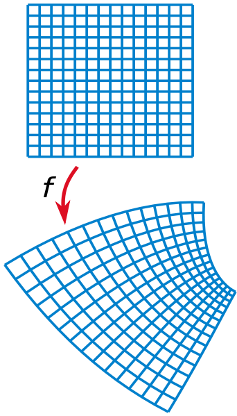
If you have read the first post on this blog, then you have seen this illustration already. Let me therefore present something better. The image below illustrates the function w = f(z) = z2 or, vice versa, the function z = √w = w1/2 (i.e. the square root of w). Indeed, that’s a very well-behaved function in the complex plane: every complex number (including negative real numbers) has two square roots in the complex plane, and so that’s what is shown below.
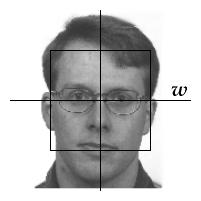
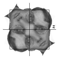
Huh? What’s this?
It’s simple: the illustration above uses color (in this case, a simple gray scale only really) to connect the points in the square region of the domain (i.e. the z plane) with an equally square region in the w plane (i.e. the image of the square region in the z plane). You can verify the properties of the z = w1/2 function indeed. At z=i we easily recognize a spot on the right ear of this person: it’s the w=−1 point in the w plane. Now, the same spot is found at z=−i. This reflects the fact that i2 = (-i)2 =−1. Similarly, this guy’s mouth, which represents the region near w=−i, is found near the two square roots of −i in the z plane, which are z=±(1−i )/√2. In fact, every part of this man’s face is found at two places in the z plane, except for the spot between his eyes, which corresponds to w=0, and also to z=0 under this transformation. Finally, you can see that this transformation is holomorphic: all (local) angles are preserved. In that sense, it’s just like a conformal map of the Earth indeed. [Note, however, that I am glossing over the fact that z = w1/2 is multiple-valued: for each value of w, we have two square roots in the z-plane. That actually creates a bit of a problem when interpreting the image above. See the post scriptum at the bottom of this post for more text on this.]
[…] OK. This is fun. [And, no, it’s not me: I found this picture on the site of a Swedish guy called Hans Lundmark, and so I give him credit for making complex analysis so much fun: just Google him to find out more.] However, let’s get somewhat more serious again and ask ourselves why we’d need holomorphism?
Well… To be honest, I am not quite sure because I haven’t gone through the rest of the course material yet – or through all these other chapters in Penrose’s book (I’ve done 10 now, so there’s 24 left). That being said, I do note that, besides all of the niceties I described above (like easy solutions for contour integrals), it is also ‘nice’ that the real and imaginary parts of an analytic function automatically satisfy the Laplace equation.
Huh? Yes. Come on! I am sure you have heard about the Laplace equation in college: it is that partial differential equation which we encounter in most physics problems. In two dimensions (i.e. in the complex plane), it’s the condition that δ2f/δx2 + δ2f/δy2 equals zero. It is a condition which pops us in electrostatics, fluid dynamics and many other areas of physical research, and I am sure you’ve seen simple examples of it.
So, this fact alone (i.e. the fact that analytic functions pop up everywhere in physics) should be justification enough in itself I guess. Indeed, the first nine chapters of Brown and Churchill’s course are only there because of the last three, which focus on applications of complex analysis in physics. But is there anything more to it?
Of course there is. Roger Penrose would not dedicate more than 200 pages to all of the above if it was not for more serious stuff than some college-level problems in physics, or to explain fluid dynamics or electrostatics. Indeed, after explaining why hypercomplex numbers (such as quaternions) are less useful than one might expect (Chapter 11 of his Road to Reality is about hypercomplex numbers and why they are useful/not useful), he jumps straight into the study of higher-dimensional manifolds (Chapter 12) and symmetry groups (Chapter 13). Now I don’t understand anything of that, as yet that is, but I sure do understand I’ll need to work my way through it if I ever want to understand what follows after: spacetime and Minkowskian geometry, quantum algebra and quantum field theory, and then the truly exotic stuff, such as supersymmetry and string theory. [By the way, from what I just gathered from the Internet, string theory has not been affected by the experimental confirmation of the existence of the Higgs particle, as it is said to be compatible with the so-called Standard Model.]
So, onwards we go! I’ll keep you posted. However, as I look at that (long) list of MIT courses, it may take some time before you hear from me again. 🙂
Post scriptum:
The nice picture of this Swedish guy is also useful to illustrate the issue of multiple-valuedness, which is an issue that pops up almost everywhere when you’re dealing with complex functions. Indeed, if we write w in its polar form w = reiθ, then its square root can be written as z = w1/2 = (√r)ei(θ/2+kπ), with k equal to either 0 or 1. So we have two square roots indeed for each w: each root has a length (i.e. its modulus or absolute value) equal to √r (i.e the positive square root of r) but their arguments are θ/2 and θ/2 + π respectively, and so that’s not the same. It means that, if z is a square root of some w in the w plane, then -z will also be a square root of w. Indeed, if the argument of z is equal to θ/2, then the argument of -z will be π/2 + π = π/2 + π – 2π = π/2 – π (we just rotate the vector by 180 degrees, which corresponds to a reflection through the origin). It means that, as we let the vector w = reiθ move around the origin – so if we let θ make a full circle starting from, let’s say, -π/2 (take the value w = –i for instance, i.e. near the guy’s mouth) – then the argument of the image of w will only go from (1/2)(-π/2) = -π/4 to (1/2)(-π/2 + 2π) = 3π/4. These two angles, i.e. -π/4 and 3π/4, correspond to the diagonal y=-x in the complex plane, and you can see that, as we go from -π/4 to 3π/4 in the z-plane, the image over this 180 degree swoop does cover every feature of this guy’s face – and here I mean not half of the guy’s face, but all of it. Continuing in the same direction (i.e. counterclockwise) from 3π/4 back to -π/4 just repeats the image. I will leave it to you to find out what happens with the angles on the two symmetry axes (y = x and y = -x).
