Light and matter

Pre-scriptum (dated 26 June 2020): This post does not seem to have suffered from the attack by the dark force. However, my views on the nature of light and matter have evolved as part of my explorations of a more realist (classical) explanation of quantum mechanics. If you are reading this, then you are probably looking for not-to-difficult reading. In that case, I would suggest you read my re-write of Feynman’s introductory lecture to QM. If you want something shorter, you can also read my paper on what I believe to be the true Principles of Physics.

Original post:

In my previous post, I discussed the de Broglie wave of a photon. It’s usually referred to as ‘the’ wave function (or the psi function) but, as I explained, for every psi – i.e. the position-space wave function Ψ(x ,t) – there is also a phi – i.e. the momentum-space wave function Φ(p, t).

In that post, I also compared it – without much formalism – to the de Broglie wave of ‘matter particles’. Indeed, in physics, we look at ‘stuff’ as being made of particles and, while the taxonomy of the particle zoo of the Standard Model of physics is rather complicated, one ‘taxonomic’ principle stands out: particles are either matter particles (known as fermions) or force carriers (known as bosons). It’s a strict separation: either/or. No split personalities.

A quick overview before we start…

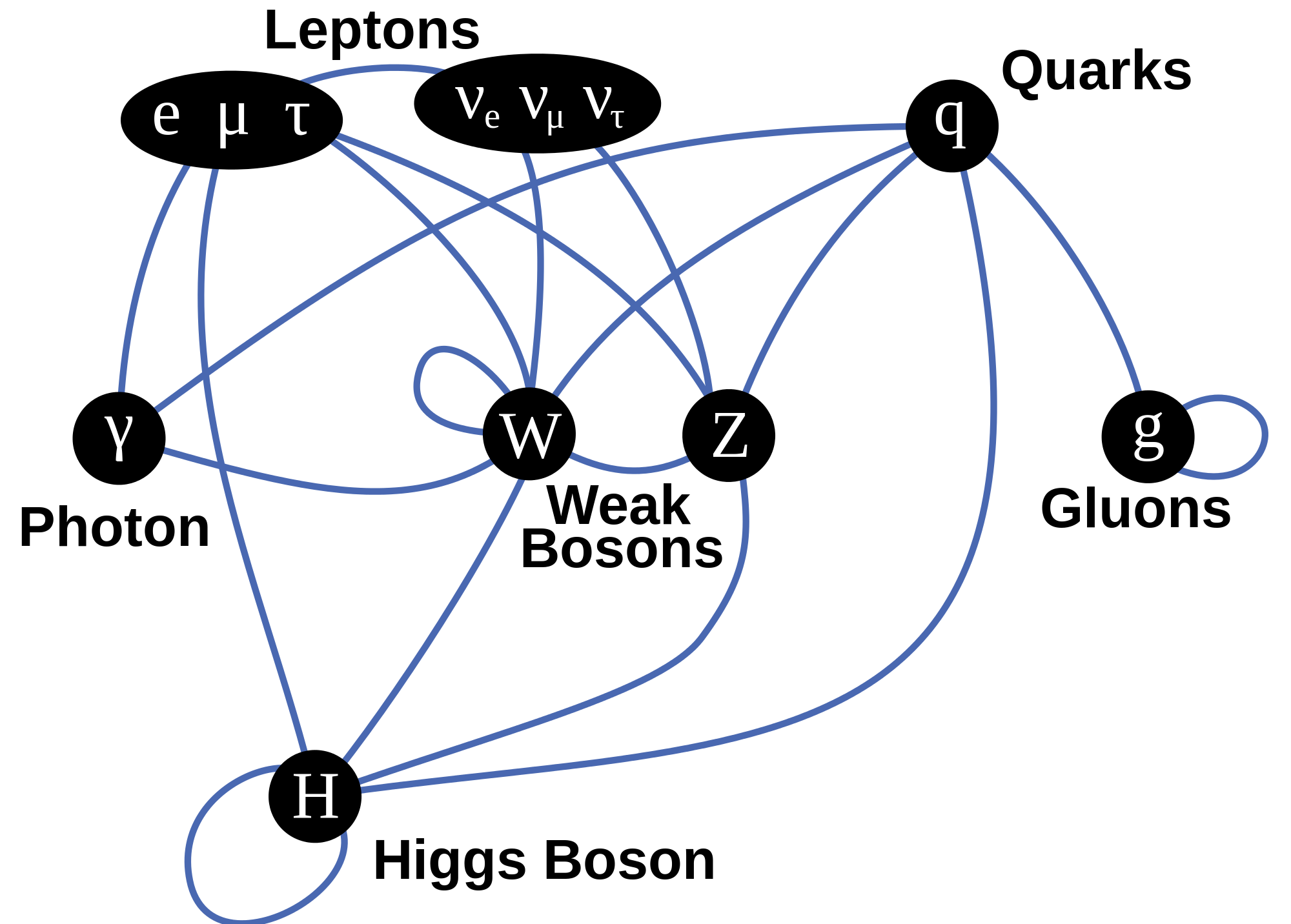
Wikipedia’s overview of particles in the Standard Model (including the latest addition: the Higgs boson) illustrates this fundamental dichotomy in nature: we have the matter particles (quarks and leptons) on one side, and the bosons (i.e. the force carriers) on the other side.

Don’t be put off by my remark on the particle zoo: it’s a term coined in the 1960s, when the situation was quite confusing indeed (like more than 400 ‘particles’). However, the picture is quite orderly now. In fact, the Standard Model put an end to the discovery of ‘new’ particles, and it’s been stable since the 1970s, as experiments confirmed the reality of quarks. Indeed, all resistance to Gell-Man’s quarks and his flavor and color concepts – which are just words to describe new types of ‘charge’ – similar to electric charge but with more variety), ended when experiments by Stanford’s Linear Accelerator Laboratory (SLAC) in November 1974 confirmed the existence of the (second-generation and, hence, heavy and unstable) ‘charm’ quark (again, the names suggest some frivolity but it’s serious physical research).

As for the Higgs boson, its existence of the Higgs boson had also been predicted, since 1964 to be precise, but it took fifty years to confirm it experimentally because only something like the Large Hadron Collider could produce the required energy to find it in these particle smashing experiments – a rather crude way of analyzing matter, you may think, but so be it. [In case you harbor doubts on the Higgs particle, please note that, while CERN is the first to admit further confirmation is needed, the Nobel Prize Committee apparently found the evidence ‘evidence enough’ to finally award Higgs and others a Nobel Prize for their ‘discovery’ fifty years ago – and, as you know, the Nobel Prize committee members are usually rather conservative in their judgment. So you would have to come up with a rather complex conspiracy theory to deny its existence.]

Also note that the particle zoo is actually less complicated than it looks at first sight: the (composite) particles that are stable in our world – this world – consist of three quarks only: a proton consists of two up quarks and one down quark and, hence, is written as uud., and a neutron is two down quarks and one up quark: udd. Hence, for all practical purposes (i.e. for our discussion how light interacts with matter), only the so-called first generation of matter-particles – so that’s the first column in the overview above – are relevant.

All the particles in the second and third column are unstable. That being said, they survive long enough – a muon disintegrates after 2.2 millionths of a second (on average) – to deserve the ‘particle’ title, as opposed to a ‘resonance’, whose lifetime can be as short as a billionth of a trillionth of a second – but we’ve gone through these numbers before and so I won’t repeat that here. Why do we need them? Well… We don’t, but they are a by-product of our world view (i.e. the Standard Model) and, for some reason, we find everything what this Standard Model says should exist, even if most of the stuff (all second- and third-generation matter particles, and all these resonances, vanish rather quickly – but so that also seems to be consistent with the model). [As for a possible fourth (or higher) generation, Feynman didn’t exclude it when he wrote his 1985 Lectures on quantum electrodynamics, but, checking on Wikipedia, I find the following: “According to the results of the statistical analysis by researchers from CERN and the Humboldt University of Berlin, the existence of further fermions can be excluded with a probability of 99.99999% (5.3 sigma).” If you want to know why… Well… Read the rest of the Wikipedia article. It’s got to do with the Higgs particle.]

As for the (first-generation) neutrino in the table – the only one which you may not be familiar with – these are very spooky things but – I don’t want to scare you – relatively high-energy neutrinos are going through your and my my body, right now and here, at a rate of some hundred trillion per second. They are produced by stars (stars are huge nuclear fusion reactors, remember?), and also as a by-product of these high-energy collisions in particle accelerators of course. But they are very hard to detect: the first trace of their existence was found in 1956 only – 26 years after their existence had been postulated: the fact that Wolfgang Pauli proposed their existence in 1930 to explain how beta decay could conserve energy, momentum and spin (angular momentum) demonstrates not only the genius but also the confidence of these early theoretical quantum physicists. Most neutrinos passing through Earth are produced by our Sun. Now they are being analyzed more routinely. The largest neutrino detector on Earth is called IceCube. It sits on the South Pole – or under it, as it’s suspended under the Antarctic ice, and it regularly captures high-energy neutrinos in the range of 1 to 10 TeV. 

Let me – to conclude this introduction – just quickly list and explain the bosons (i.e the force carriers) in the table above:

1. Of all of the bosons, the photon (i.e. the topic of this post), is the most straightforward: there is only type of photon, even if it comes in different possible states of polarization.

[…]

I should probably do a quick note on polarization here – even if all of the stuff that follows will make abstraction of it. Indeed, the discussion on photons that follows (largely adapted from Feynman’s 1985 Lectures on Quantum Electrodynamics) assumes that there is no such thing as polarization – because it would make everything even more complicated. The concept of polarization (linear, circular or elliptical) has a direct physical interpretation in classical mechanics (i.e. light as an electromagnetic wave). In quantum mechanics, however, polarization becomes a so-called qubit (quantum bit): leaving aside so-called virtual photons (these are short-range disturbances going between a proton and an electron in an atom – effectively mediating the electromagnetic force between them), the property of polarization comes in two basis states (0 and 1, or left and right), but these two basis states can be superposed. In ket notation: if ¦0〉 and ¦1〉 are the basis states, then any linear combination α·¦0〉 + ß·¦1〉 is also a valid state provided│α│² + │β│² = 1, in line with the need to get probabilities that add up to one.

In case you wonder why I am introducing these kets, there is no reason for it, except that I will be introducing some other tools in this post – such as Feynman diagrams – and so that’s all. In order to wrap this up, I need to note that kets are used in conjunction with bras. So we have a bra-ket notation: the ket gives the starting condition, and the bra – denoted as 〈 ¦ – gives the final condition. They are combined in statements such as 〈 particle arrives at x¦particle leaves from s〉 or – in short – 〈 x¦s〉 and, while x and s would have some real-number value, 〈 x¦s〉 would denote the (complex-valued) probability amplitude associated wit the event consisting of these two conditions (i.e the starting and final condition).

But don’t worry about it. This digression is just what it is: a digression. Oh… Just make a mental note that the so-called virtual photons (the mediators that are supposed to keep the electron in touch with the proton) have four possible states of polarization – instead of two. They are related to the four directions of space (x, y and z) and time (t). 🙂

2. Gluons, the exchange particles for the strong force, are more complicated: they come in eight so-called colors. In practice, one should think of these colors as different charges, but so we have more elementary charges in this case than just plus or minus one (±1) – as we have for the electric charge. So it’s just another type of qubit in quantum mechanics.

[Note that the so-called elementary ±1 values for electric charge are not really elementary: it’s –1/3 (for the down quark, and for the second- and third-generation strange and bottom quarks as well) and +2/3 (for the up quark as well as for the second- and third-generation charm and top quarks). That being said, electric charge takes two values only, and the ±1 value is easily found from a linear combination of the –1/3 and +2/3 values.]

3. Z and W bosons carry the so-called weak force, aka as Fermi’s interaction: they explain how one type of quark can change into another, thereby explaining phenomena such as beta decay. Beta decay explains why carbon-14 will, after a very long time (as compared to the ‘unstable’ particles mentioned above), spontaneously decay into nitrogen-14. Indeed, carbon-12 is the (very) stable isotope, while carbon-14 has a life-time of 5,730 ± 40 years ‘only’  (so one can’t call carbon-12 ‘unstable’: perhaps ‘less stable’ will do) and, hence, measuring how much carbon-14 is left in some organic substance allows us to date it (that’s what (radio)carbon-dating is about). As for the name, a beta particle can refer to an electron or a positron, so we can have β^– decay (e.g. the above-mentioned carbon-14 decay) as well as β⁺ decay (e.g. magnesium-23 into sodium-23). There’s also alpha and gamma decay but that involves different things. 

As you can see from the table, W^± and Z⁰ bosons are very heavy (157,000 and 178,000 times heavier than a electron!), and W^± carry the (positive or negative) electric charge. So why don’t we see them? Well… They are so short-lived that we can only see a tiny decay width, just a very tiny little trace, so they resemble resonances in experiments. That’s also the reason why we see little or nothing of the weak force in real-life: the force-carrying particles mediating this force don’t get anywhere.

4. Finally, as mentioned above, the Higgs particle – and, hence, of the associated Higgs field – had been predicted since 1964 already but its existence was only (tentatively) experimentally confirmed last year. The Higgs field gives fermions, and also the W and Z bosons, mass (but not photons and gluons), and – as mentioned above – that’s why the weak force has such short range as compared to the electromagnetic and strong forces. Note, however, that the Higgs particle does actually not explain the gravitational force, so it’s not the (theoretical) graviton and there is no quantum field theory for the gravitational force as yet. Just Google it and you’ll quickly find out why: there’s theoretical as well as practical (experimental) reasons for that.

The Higgs field stands out from the other force fields because it’s a scalar field (as opposed to a vector field). However, I have no idea how this so-called Higgs mechanism (i.e. the interaction with matter particles (i.e. with the quarks and leptons, but not directly with neutrinos it would seem from the diagram below), with W and Z bosons, and with itself – but not with the massless photons and gluons) actually works. But then I still have a very long way to go on this Road to Reality.

In any case… The topic of this post is to discuss light and its interaction with matter – not the weak or strong force, nor the Higgs field.

Let’s go for it.

Amplitudes, probabilities and observable properties

Being born a boson or a fermion makes a big difference. That being said, both fermions and bosons are wavicles described by a complex-valued psi function, colloquially known as the wave function. To be precise, there will be several wave functions, and the square of their modulus (sorry for the jargon) will give you the probability of some observable property having a value in some relevant range, usually denoted by Δ. [I also explained (in my post on Bose and Fermi) how the rules for combining amplitudes differ for bosons versus fermions, and how that explains why they are what they are: matter particles occupy space, while photons not only can but also like to crowd together in, for example, a powerful laser beam. I’ll come back on that.]

For all practical purposes, relevant usually means ‘small enough to be meaningful’. For example, we may want to calculate the probability of detecting an electron in some tiny spacetime interval (Δx, Δt). [Again, ‘tiny’ in this context means small enough to be relevant: if we are looking at a hydrogen atom (whose size is a few nanometer), then Δx is likely to be a cube or a sphere with an edge or a radius of a few picometer only (a picometer is a thousandth of a nanometer, so it’s a millionth of a millionth of a meter); and, noting that the electron’s speed is approximately 2200 km per second… Well… I will let you calculate a relevant Δt. :-)]

If we want to do that, then we will need to square the modulus of the corresponding wave function Ψ(x, t). To be precise, we will have to do a summation of all the values │Ψ(x, t)│² over the interval and, because x and t are real (and, hence, continuous) numbers, that means doing some integral (because an integral is the continuous version of a sum).

But that’s only one example of an observable property: position. There are others. For example, we may not be interested in the particle’s exact position but only in its momentum or energy. Well, we have another wave function for that: the momentum wave function Φ(x ,t). In fact, if you looked at my previous posts, you’ll remember the two are related because they are conjugate variables: Fourier transforms duals of one another. A less formal way of expressing that is to refer to the uncertainty principle. But this is not the time to repeat things.

The bottom line is that all particles travel through spacetime with a backpack full of complex-valued wave functions. We don’t know who and where these particles are exactly, and so we can’t talk to them – but we can e-mail God and He’ll send us the wave function that we need to calculate some probability we are interested in because we want to check – in all kinds of experiments designed to fool them – if it matches with reality.

As mentioned above, I highlighted the main difference between bosons and fermions in my Bose and Fermi post, so I won’t repeat that here. Just note that, when it comes to working with those probability amplitudes (that’s just another word for these psi and phi functions), it makes a huge difference: fermions and bosons interact very differently. Bosons are party particles: they like to crowd and will always welcome an extra one. Fermions, on the other hand, will exclude each other: that’s why there’s something referred to as the Fermi exclusion principle in quantum mechanics. That’s why fermions make matter (matter needs space) and bosons are force carriers (they’ll just call friends to help when the load gets heavier).

Light versus matter: Quantum Electrodynamics

OK. Let’s get down to business. This post is about light, or about light-matter interaction. Indeed, in my previous post (on Light), I promised to say something about the amplitude of a photon to go from point A to B (because – as I wrote in my previous post – that’s more ‘relevant’, when it comes to explaining stuff, than the amplitude of a photon to actually be at point x at time t), and so that’s what I will do now.

In his 1985 Lectures on Quantum Electrodynamics (which are lectures for the lay audience), Feynman writes the amplitude of a photon to go from point A to B as P(A to B) – and the P stands for photon obviously, not for probability. [I am tired of repeating that you need to square the modulus of an amplitude to get a probability but – here you are – I have said it once more.] That’s in line with the other fundamental wave function in quantum electrodynamics (QED): the amplitude of an electron to go from A to B, which is written as E(A to B). [You got it: E just stands for electron, not for our electric field vector.]

I also talked about the third fundamental amplitude in my previous post: the amplitude of an electron to absorb or emit a photon. So let’s have a look at these three. As Feynman says: ““Out of these three amplitudes, we can make the whole world, aside from what goes on in nuclei, and gravitation, as always!” 

Well… Thank you, Mr Feynman: I’ve always wanted to understand the World (especially if you made it).

The photon-electron coupling constant j

Let’s start with the last of those three amplitudes (or wave functions): the amplitude of an electron to absorb or emit a photon. Indeed, absorbing or emitting makes no difference: we have the same complex number for both. It’s a constant – denoted by j (for junction number) – equal to –0.1 (a bit less actually but it’s good enough as an approximation in the context of this blog).

Huh? Minus 0.1? That’s not a complex number, is it? It is. Real numbers are complex numbers too: –0.1 is 0.1e^iπ in polar coordinates. As Feynman puts it: it’s “a shrink to about one-tenth, and half a turn.” The ‘shrink’ is the 0.1 magnitude of this vector (or arrow), and the ‘half-turn’ is the angle of π (i.e. 180 degrees). He obviously refers to multiplying (no adding here) j with other amplitudes, e.g. P(A, C) and E(B, C) if the coupling is to happen at or near C. And, as you’ll remember, multiplying complex numbers amounts to adding their phases, and multiplying their modulus (so that’s adding the angles and multiplying lengths).

Let’s introduce a Feynman diagram at this point – drawn by Feynman himself – which shows three possible ways of two electrons exchanging a photon. We actually have two couplings here, and so the combined amplitude will involve two j‘s. In fact, if we label the starting point of the two lines representing our electrons as 1 and 2 respectively, and their end points as 3 and 4, then the amplitude for these events will be given by:

E(1 to 5)·j·E(5 to 3)·E(2 to 6)·j·E(6 to 3)

 As for how that j factor works, please do read the caption of the illustration below: the same j describes both emission as well as absorption. It’s just that we have both an emission as well as an as absorption here, so we have a j² factor here, which is less than 0.1·0.1 = 0.01. At this point, it’s worth noting that it’s obvious that the amplitudes we’re talking about here – i.e. for one possible way of an exchange like the one below happening – are very tiny. They only become significant when we add many of these amplitudes, which – as explained below – is what has to happen: one has to consider all possible paths, calculate the amplitudes for them (through multiplication), and then add all these amplitudes, to then – finally – square the modulus of the combined ‘arrow’ (or amplitude) to get some probability of something actually happening. [Again, that’s the best we can do: calculate probabilities that correspond to experimentally measured occurrences. We cannot predict anything in the classical sense of the word.]

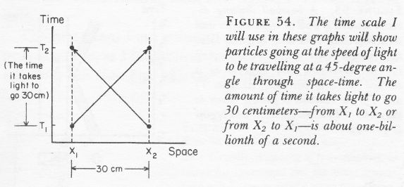
A Feynman diagram is not just some sketchy drawing. For example, we have to care about scales: the distance and time units are equivalent (so distance would be measured in light-seconds or, else, time would be measured in units equivalent to the time needed for light to travel one meter). Hence, particles traveling through time (and space) – from the bottom of the graph to the top – will usually not  be traveling at an angle of more than 45 degrees (as measured from the time axis) but, from the graph above, it is clear that photons do. [Note that electrons moving through spacetime are represented by plain straight lines, while photons are represented by wavy lines. It’s just a matter of convention.]

More importantly, a Feynman diagram is a pictorial device showing what needs to be calculated and how. Indeed, with all the complexities involved, it is easy to lose track of what should be added and what should be multiplied, especially when it comes to much more complicated situations like the one described above (e.g. making sense of a scattering event). So, while the coupling constant j (aka as the ‘charge’ of a particle – but it’s obviously not the electric charge) is just a number, calculating an actual E(A to B) amplitudes is not easy – not only because there are many different possible routes (paths) but because (almost) anything can happen. Let’s have a closer look at it.

E(A to B)

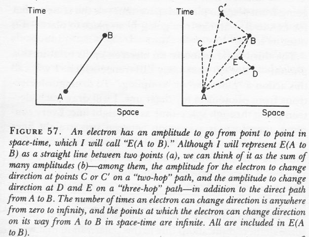
As Feynman explains in his 1985 QED Lectures: “E(A to B) can be represented as a giant sum of a lot of different ways an electron can go from point A to B in spacetime: the electron can take a ‘one-hop flight’, going directly from point A to B; it could take a ‘two-hop flight’, stopping at an intermediate point C; it could take a ‘three-hop flight’ stopping at points D and E, and so on.”

Fortunately, the calculation re-uses known values: the amplitude for each ‘hop’ – from C to D, for example – is P(F to G) – so that’s the amplitude of a photon (!) to go from F to G – even if we are talking an electron here. But there’s a difference: we also have to multiply the amplitudes for each ‘hop’ with the amplitude for each ‘stop’, and that’s represented by another number – not j but n². So we have an infinite series of terms for E(A to B): P(A to B) + P(A to C)·n²·P(C to B) + P(A to D)·n²·P(D to E)·n²·P(E to B) + … for all possible intermediate points C, D, E, and so on, as per the illustration below.

You’ll immediately ask: what’s the value of n? It’s quite important to know it, because we want to know how big these n², n⁴ etcetera terms are. I’ll be honest: I have not come to terms with that yet. According to Feynman (QED, p. 125), it is the ‘rest mass’ of an ‘ideal’ electron: an ‘ideal’ electron is an electron that doesn’t know Feynman’s amplitude theory and just goes from point to point in spacetime using only the direct path. 🙂 Hence, it’s not a probability amplitude like j: a proper probability amplitude will always have a modulus less than 1, and so when we see exponential terms like j², j⁴,… we know we should not be all that worried – because these sort of vanish (go to zero) for sufficiently large exponents. For E(A to B), we do not have such vanishing terms. I will not dwell on this right here, but I promise to discuss it in the Post Scriptum of this post. The frightening possibility is that n might be a number larger than one.

[As we’re freewheeling a bit anyway here, just a quick note on conventions: I should not be writing j in bold-face, because it’s a (complex- or real-valued) number and symbols representing numbers are usually not written in bold-face: vectors are written in bold-face. So, while you can look at a complex number as a vector, well… It’s just one of these inconsistencies I guess. The problem with using bold-face letters to represent complex numbers (like amplitudes) is that they suggest that the ‘dot’ in a product (e.g. j·j) is an actual dot project (aka as a scalar product or an inner product) of two vectors. That’s not the case. We’re multiplying complex numbers here, and so we’re just using the standard definition of a product of complex numbers. This subtlety probably explains why Feynman prefers to write the above product as P(A to B) + P(A to C)*n²*P(C to B) + P(A to D)*n²*P(D to E)*n²*P(E to B) + … But then I find that using that asterisk to represent multiplication is a bit funny (although it’s a pretty common thing in complex math) and so I am not using it. Just be aware that a dot in a product may not always mean the same type of multiplication: multiplying complex numbers and multiplying vectors is not the same. […] And I won’t write j in bold-face anymore.]

P(A to B)

Regardless of the value for n, it’s obvious we need a functional form for P(A to B), because that’s the other thing (other than n) that we need to calculate E(A to B). So what’s the amplitude of a photon to go from point A to B?

Well… The function describing P(A to B) is obviously some wave function – so that’s a complex-valued function of x and t. It’s referred to as a (Feynman) propagator: a propagator function gives the probability amplitude for a particle to travel from one place to another in a given time, or to travel with a certain energy and momentum. [So our function for E(A to B) will be a propagator as well.] You can check out the details on it on Wikipedia. Indeed, I could insert the formula here, but believe me if I say it would only confuse you. The points to note is that:

1. The propagator is also derived from the wave equation describing the system, so that’s some kind of differential equation which incorporates the relevant rules and constraints that apply to the system. For electrons, that’s the Schrödinger equation I presented in my previous post. For photons… Well… As I mentioned in my previous post, there is ‘something similar’ for photons – there must be – but I have not seen anything that’s equally ‘simple’ as the Schrödinger equation for photons. [I have Googled a bit but it’s obvious we’re talking pretty advanced quantum mechanics here – so it’s not the QM-101 course that I am currently trying to make sense of.] 
2. The most important thing (in this context at least) is that the key variable in this propagator (i.e. the Feynman propagator for the photon) is I: that spacetime interval which I mentioned in my previous post already:

I = Δr² – Δt² =  (z₂– z₁)² + (y₂– y₁)² + (x₂– x₁)² – (t₂– t₁)²

In this equation, we need to measure the time and spatial distance between two points in spacetime in equivalent units (these ‘points’ are usually referred to as four-vectors), so we’d use light-seconds for the unit of distance or, for the unit of time, the time it takes for light to travel one meter. [If we don’t want to transform time or distance scales, then we have to write I as I = c²Δt² – Δr².] Now, there are three types of intervals:

1. For time-like intervals, we have a negative value for I, so Δt² > Δr². For two events separated by a time-like interval, enough time passes between them so there could be a cause–effect relationship between the two events. In a Feynman diagram, the angle between the time axis and the line between the two events will be less than 45 degrees from the vertical axis. The traveling electrons in the Feynman diagrams above are an example.
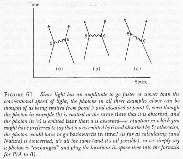
2. For space-like intervals, we have a positive value for I, so Δt² < Δr². Events separated by space-like intervals cannot possibly be causally connected. The photons traveling between point 5 and 6 in the first Feynman diagram are an example, but then photons do have amplitudes to travel faster than light.
3. Finally, for light-like intervals, I = 0, or Δt² = Δr². The points connected by the 45-degree lines in the illustration below (which Feynman uses to introduce his Feynman diagrams) are an example of points connected by light-like intervals.

[Note that we are using the so-called space-like convention (+++–) here for I. There’s also a time-like convention, i.e. with +––– as signs: I = Δt² – Δr² so just check when you would consult other sources on this (which I recommend) and if you’d feel I am not getting the signs right.]

Now, what’s the relevance of this? To calculate P(A to B), we have to add the amplitudes for all possible paths that the photon can take, and not in space, but in spacetime. So we should add all these vectors (or ‘arrows’ as Feynman calls them) – an infinite number of them really. In the meanwhile, you know it amounts to adding complex numbers, and that infinite sums are done by doing integrals, but let’s take a step back: how are vectors added?

Well…That’s easy, you’ll say… It’s the parallelogram rule… Well… Yes. And no. Let me take a step back here to show how adding a whole range of similar amplitudes works.

The illustration below shows a bunch of photons – real or imagined – from a source above a water surface (the sun for example), all taking different paths to arrive at a detector under the water (let’s say some fish looking at the sky from under the water). In this case, we make abstraction of all the photons leaving at different times and so we only look at a bunch that’s leaving at the same point in time. In other words, their stopwatches will be synchronized (i.e. there is no phase shift term in the phase of their wave function) – let’s say at 12 o’clock when they leave the source. [If you think this simplification is not acceptable, well… Think again.]

When these stopwatches hit the retina of our poor fish’s eye (I feel we should put a detector there, instead of a fish), they will stop, and the hand of each stopwatch represents an amplitude: it has a modulus (its length) – which is assumed to be the same because all paths are equally likely (this is one of the first principles of QED) – but their direction is very different. However, by now we are quite familiar with these operations: we add all the ‘arrows’ indeed (or vectors or amplitudes or complex numbers or whatever you want to call them) and get one big final arrow, shown at the bottom – just above the caption. Look at it very carefully.

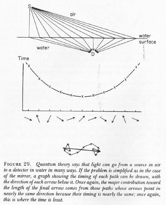
If you look at the so-called contribution made by each of the individual arrows, you can see that it’s the arrows associated with the path of least time and the paths immediately left and right of it that make the biggest contribution to the final arrow. Why? Because these stopwatches arrive around the same time and, hence, their hands point more or less in the same direction. It doesn’t matter what direction – as long as it’s more or less the same.

[As for the calculation of the path of least time, that has to do with the fact that light is slowed down in water. Feynman shows why in his 1985 Lectures on QED, but I cannot possibly copy the whole book here ! The principle is illustrated below.]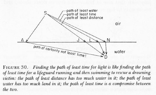  

So, where are we? This digressions go on and on, don’t they? Let’s go back to the main story: we want to calculate P(A to B), remember?

As mentioned above, one of the first principles in QED is that all paths – in spacetime – are equally likely. So we need to add amplitudes for every possible path in spacetime using that Feynman propagator function. You can imagine that will be some kind of integral which you’ll never want to solve. Fortunately, Feynman’s disciples have done that for you already. The results is quite predictable: the grand result is that light has a tendency to travel in straight lines and at the speed of light.

WHAT!? Did Feynman get a Nobel prize for trivial stuff like that?

Yes. The math involved in adding amplitudes over all possible paths not only in space but also in time uses the so-called path integral formulation of quantum mechanics and so that’s got Feynman’s signature on it, and that’s the main reason why he got this award – together with Julian Schwinger and Sin-Itiro Tomonaga: both much less well known than Feynman, but so they shared the burden. Don’t complain about it. Just take a look at the ‘mechanics’ of it.

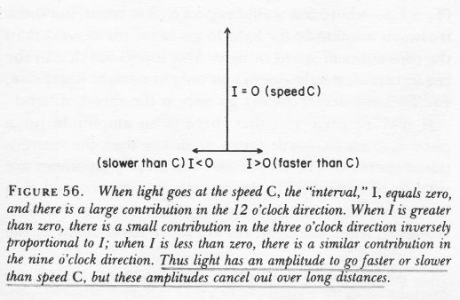
We already mentioned that the propagator has the spacetime interval I in its denominator. Now, the way it works is that, for values of I equal or close to zero, so the paths that are associated with light-like intervals, our propagator function will yield large contributions in the ‘same’ direction (wherever that direction is), but for the spacetime intervals that are very much time- or space-like, the magnitude of our amplitude will be smaller and – worse – our arrow will point in the ‘wrong’ direction. In short, the arrows associated with the time- and space-like intervals don’t add up to much, especially over longer distances. [When distances are short, there are (relatively) few arrows to add, and so the probability distribution will be flatter: in short, the likelihood of having the actual photon travel faster or slower than speed is higher.]

Conclusion

Does this make sense? I am not sure, but I did what I promised to do. I told you how P(A to B) gets calculated; and from the formula for E(A to B), it is obvious that we can then also calculate E(A to B) provided we have a value for n. However, that value n is determined experimentally, just like the value of j, in order to ensure this amplitude theory yields probabilities that match the probabilities we observe in all kinds of crazy experiments that try to prove or disprove the theory; and then we can use these three amplitude formulas “to make the whole world”, as Feynman calls it, except the stuff that goes on inside of nuclei (because that’s the domain of the weak and strong nuclear force) and gravitation, for which we have a law (Newton’s Law) but no real ‘explanation’. [Now, you may wonder if this QED explanation of light is really all that good, but Mr Feynman thinks it is, and so I have no reason to doubt that – especially because there’s surely not anything more convincing lying around as far as I know.]

So what remains to be told? Lots of things, even within the realm of expertise of quantum electrodynamics. Indeed, Feynman applies the basics as described above to a number of real-life phenomena – quite interesting, all of it ! – but, once again, it’s not my goal to copy all of his Lectures here. [I am only hoping to offer some good summaries of key points in some attempt to convince myself that I am getting some of it at least.] And then there is the strong force, and the weak force, and the Higgs field, and so and so on. But that’s all very strange and new territory which I haven’t even started to explore. I’ll keep you posted as I am making my way towards it.

Post scriptum: On the values of j and n

In this post, I promised I would write something about how we can find j and n because I realize it would just amount to copy three of four pages out of that book I mentioned above, and which inspired most of this post. Let me just say something more about that remarkable book, and then quote a few lines on what the author of that book – the great Mr Feynman ! – thinks of the math behind calculating these two constants (the coupling constant j, and the ‘rest mass’ of an ‘ideal’ electron). Now, before I do that, I should repeat that he actually invented that math (it makes use of a mathematical approximation method called perturbation theory) and that he got a Nobel Prize for it.

First, about the book. Feynman’s 1985 Lectures on Quantum Electrodynamics are not like his 1965 Lectures on Physics. The Lectures on Physics are proper courses for undergraduate and even graduate students in physics. This little 1985 book on QED is just a series of four lectures for a lay audience, conceived in honor of Alix G. Mautner. She was a friend of Mr Feynman’s who died a few years before he gave and wrote these ‘lectures’ on QED. She had a degree in English literature and would ask Mr Feynman regularly to explain quantum mechanics and quantum electrodynamics in a way she would understand. While they had known each other for about 22 years, he had apparently never taken enough time to do so, as he writes in his Introduction to these Alix G. Mautner Memorial Lectures: “So here are the lectures I really [should have] prepared for Alix, but unfortunately I can’t tell them to her directly, now.”

The great Richard Phillips Feynman himself died only three years later, in February 1988 – not of one but two rare forms of cancer. He was only 69 years old when he died. I don’t know if he was aware of the cancer(s) that would kill him, but I find his fourth and last lecture in the book, Loose Ends, just fascinating. Here we have a brilliant mind deprecating the math that earned him a Nobel Prize and without which the Standard Model would be unintelligible. I won’t try to paraphrase him. Let me just quote him. [If you want to check the quotes, the relevant pages are page 125 to 131):

The math behind calculating these constants] is a “dippy process” and “having to resort to such hocus-pocus has prevented us from proving that the theory of quantum electrodynamics is mathematically self-consistent“. He adds: “It’s surprising that the theory still hasn’t been proved self-consistent one way or the other by now; I suspect that renormalization [“the shell game that we play to find n and j” as he calls it]  is not mathematically legitimate.” […] Now, Mr Feynman writes this about quantum electrodynamics, not about “the rest of physics” (and so that’s quantum chromodynamics (QCD) – the theory of the strong interactions – and quantum flavordynamics (QFD) – the theory of weak interactions) which, he adds, “has not been checked anywhere near as well as electrodynamics.” 

That’s a pretty damning statement, isn’t it? In one of my other posts (see: The End of the Road to Reality?), I explore these comments a bit. However, I have to admit I feel I really need to get back to math in order to appreciate these remarks. I’ve written way too much about physics anyway now (as opposed to the my first dozen of posts – which were much more math-oriented). So I’ll just have a look at some more stuff indeed (such as perturbation theory), and then I’ll get back blogging. Indeed, I’ve written like 20 posts or so in a few months only – so I guess I should shut up for while now !

In the meanwhile, you’re more than welcome to comment of course !