Re-visiting electron orbitals

Pre-script (dated 26 June 2020): This post got mutilated by the removal of some material by the dark force. You should be able to follow the main story line, however. If anything, the lack of illustrations might actually help you to think things through for yourself. In any case, we now have different views on these concepts as part of our realist interpretation of quantum mechanics, so we recommend you read our recent papers instead of these old blog posts.

Original post:

One of the pieces I barely gave a glance when reading Feynman’s Lectures over the past few years, was the derivation of the non-spherical electron orbitals for the hydrogen atom. It just looked like a boring piece of math – and I thought the derivation of the s-orbitals – the spherically symmetrical ones – was interesting enough already. To some extent, it is – but there is so much more to it. When I read it now, the derivation of those p-, d-, f– etc. orbitals brings all of the weirdness of quantum mechanics together and, while doing so, also provides for a deeper understanding of all of the ideas and concepts we’re trying to get used to. In addition, Feynman’s treatment of the matter is actually much shorter than what you’ll find in other textbooks, because… Well… As he puts it, he takes a shortcut. So let’s try to follow the bright mind of our Master as he walks us through it.

You’ll remember – if not, check it out again – that we found the spherically symmetric solutions for Schrödinger’s equation for our hydrogen atom. Just to be make sure, Schrödinger’s equation is a differential equation – a condition we impose on the wavefunction for our electron – and so we need to find the functional form for the wavefunctions that describe the electron orbitals. [Quantum math is so confusing that it’s often good to regularly think of what it is that we’re actually trying to do. :-)] In fact, that functional form gives us a whole bunch of solutions – or wavefunctions – which are defined by three quantum numbers: n, l, and m. The parameter n corresponds to an energy level (E_n), l is the orbital (quantum) number, and m is the z-component of the angular momentum. But that doesn’t say much. Let’s go step by step.

First, we derived those spherically symmetric solutions – which are referred to as s-states – assuming this was a state with zero (orbital) angular momentum, which we write as l = 0. [As you know, Feynman does not incorporate the spin of the electron in his analysis, which is, therefore, approximative only.] Now what exactly is a state with zero angular momentum? When everything is said and done, we are effectively trying to describe some electron orbital here, right? So that’s an amplitude for the electron to be somewhere, but then we also know it always moves. So, when everything is said and done, the electron is some circulating negative charge, right? So there is always some angular momentum and, therefore, some magnetic moment, right?

Well… If you google this question on Physics Stack Exchange, you’ll get a lot of mumbo jumbo telling you that you shouldn’t think of the electron actually orbiting around. But… Then… Well… A lot of that mumbo jumbo is contradictory. For example, one of the academics writing there does note that, while we shouldn’t think of an electron as some particle, the orbital is still a distribution which gives you the probability of actually finding the electron at some point (x,y,z). So… Well… It is some kind of circulating charge – as a point, as a cloud or as whatever. The only reasonable answer – in my humble opinion – is that l = 0 probably means there is no net circulating charge, so the movement in this or that direction must balance the movement in the other. One may note, in this regard, that the phenomenon of electron capture in nuclear reactions suggests electrons do travel through the nucleus for at least part of the time, which is entirely coherent with the wavefunctions for s-states – shown below – which tell us that the most probable (x, y, z) position for the electron is right at the center – so that’s where the nucleus is. There is also a non-zero probability for the electron to be at the center for the other orbitals (p, d, etcetera).In fact, now that I’ve shown this graph, I should quickly explain it. The three graphs are the spherically symmetric wavefunctions for the first three energy levels. For the first energy level – which is conventionally written as n = 1, not as n = 0 – the amplitude approaches zero rather quickly. For n = 2 and n = 3, there are zero-crossings: the curve passes the r-axis. Feynman calls these zero-crossing radial nodes. To be precise, the number of zero-crossings for these s-states is n − 1, so there’s none for n = 1, one for n = 2, two for n = 3, etcetera.

Now, why is the amplitude – apparently – some real-valued function here? That’s because we’re actually not looking at ψ(r, t) here but at the ψ(r) function which appears in the following break-up of the actual wavefunction ψ(r, t):

ψ(r, t) = e^{−i·(E/ħ)·t}·ψ(r)

So ψ(r) is more of an envelope function for the actual wavefunction, which varies both in space as well as in time. It’s good to remember that: I would have used another symbol, because ψ(r, t) and ψ(r) are two different beasts, really – but then physicists want you to think, right? And Mr. Feynman would surely want you to do that, so why not inject some confusing notation from time to time? 🙂 So for n = 3, for example, ψ(r) goes from positive to negative and then to positive, and these areas are separated by radial nodes. Feynman put it on the blackboard like this:I am just inserting it to compare this concept of radial nodes with the concept of a nodal plane, which we’ll encounter when discussing p-states in a moment, but I can already tell you what they are now: those p-states are symmetrical in one direction only, as shown below, and so we have a nodal plane instead of a radial node. But so I am getting ahead of myself here… 🙂Before going back to where I was, I just need to add one more thing. 🙂 Of course, you know that we’ll take the square of the absolute value of our amplitude to calculate a probability (or the absolute square – as we abbreviate it), so you may wonder why the sign is relevant at all. Well… I am not quite sure either but there’s this concept of orbital parity which you may have heard of.  The orbital parity tells us what will happen to the sign if we calculate the value for ψ for −r rather than for r. If ψ(−r) = ψ(r), then we have an even function – or even orbital parity. Likewise, if ψ(−r) = −ψ(r), then we’ll the function odd – and so we’ll have an odd orbital parity. The orbital parity is always equal to (-1)^l = ±1. The exponent l is that angular quantum number, and +1, or + tout court, means even, and -1 or just − means odd. The angular quantum number for those p-states is l = 1, so that works with the illustration of the nodal plane. 🙂 As said, it’s not hugely important but I might as well mention in passing – especially because we’ll re-visit the topic of symmetries a few posts from now. 🙂

OK. I said I would talk about states with some angular momentum (so l ≠ 0) and so it’s about time I start doing that. As you know, our orbital angular momentum l is measured in units of ħ (just like the total angular momentum J, which we’ve discussed ad nauseam already). We also know that if we’d measure its component along any direction – any direction really, but physicists will usually make sure that the z-axis of their reference frame coincides with, so we call it the z-axis 🙂 – then we will find that it can only have one of a discrete set of values m·ħ = l·ħ, (l-1)·ħ, …, -(l-1)·ħ, –l·ħ. Hence, l just takes the role of our good old quantum number j here, and m is just J_z. Likewise, I’d like to introduce l as the equivalent of J, so we can easily talk about the angular momentum vector. And now that we’re here, why not write m in bold type too, and say that m is the z-component itself – i.e. the whole vector quantity, so that’s the direction and the magnitude.

Now, we do need to note one crucial difference between j and l, or between J and l: our j could be an integer or a half-integer. In contrast, l must be some integer. Why? Well… If l can be zero, and the values of l must be separated by a full unit, then l must be 1, 2, 3 etcetera. 🙂 If this simple answer doesn’t satisfy you, I’ll refer you to Feynman’s, which is also short but more elegant than mine. 🙂 Now, you may or may not remember that the quantum-mechanical equivalent of the magnitude of a vector quantity such as l is to be calculated as √[l·(l+1)]·ħ, so if l = 1, that magnitude will be √2·ħ ≈ 1.4142·ħ, so that’s – as expected – larger than the maximum value for m, which is +1. As you know, that leads us to think of that z-component m as a projection of l. Paraphrasing Feynman, the limited set of values for m imply that the angular momentum is always “cocked” at some angle. For l = 1, that angle is either +45° or, else, −45°, as shown below.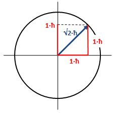What if l = 2? The magnitude of l is then equal to √[2·(2+1)]·ħ = √6·ħ ≈ 2.4495·ħ. How do we relate that to those “cocked” angles? The values of m now range from -2 to +2, with a unit distance in-between. The illustration below shows the angles. [I didn’t mention ħ any more in that illustration because, by now, we should know it’s our unit of measurement – always.]

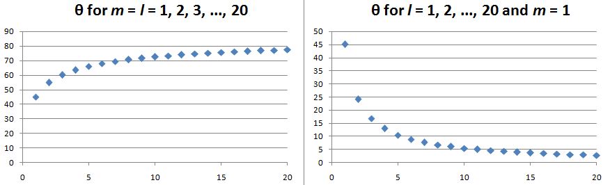
Note we’ve got a bigger circle here (the radius is about 2.45 here, as opposed to a bit more than 1.4 for m = 0). Also note that it’s not a nice cake with perfectly equal pieces. From the graph, it’s obvious that the formula for the angle is the following: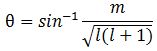It’s simple but intriguing. Needless to say, the sin ⁻¹ function is the inverse sine, also known as the arcsine. I’ve calculated the values for all m for l = 1, 2, 3, 4 and 5 below. The most interesting values are the angles for m = 1 and m = l. As the graphs underneath show, for m = 1, the values start approaching the zero angle for very large l, so there’s not much difference any more between m = ±1 and m = 1 for large values of l. What about the m = l case? Well… Believe it or not, if l becomes really large, then these angles do approach 90°. If you don’t remember how to calculate limits, then just calculate θ for some huge value for l and m. For l = m = 1,000,000, for example, you should find that θ = 89.9427…°. 🙂

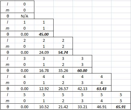
Isn’t this fascinating? I’ve actually never seen this in a textbook – so it might be an original contribution. 🙂 OK. I need to get back to the grind: Feynman’s derivation of non-symmetrical electron orbitals. Look carefully at the illustration below. If m is really the projection of some angular momentum that’s “cocked”, either at a zero-degree or, alternatively, at ±45º (for the l = 1 situation we show here) – a projection on the z-axis, that is – then the value of m (+1, 0 or -1) does actually correspond to some idea of the orientation of the space in which our electron is circulating. For m = 0, that space – think of some torus or whatever other space in which our electron might circulate – would have some alignment with the z-axis. For m = ±1, there is no such alignment. 

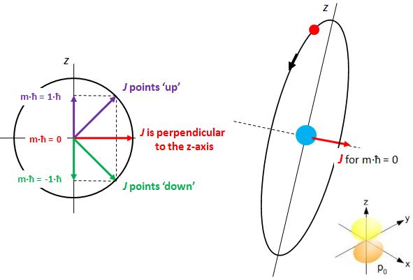
The interpretation is tricky, however, and the illustration on the right-hand side above is surely too much of a simplification: an orbital is definitely not like a planetary orbit. It doesn’t even look like a torus. In fact, the illustration in the bottom right corner, which shows the probability density, i.e. the space in which we are actually likely to find the electron, is a picture that is much more accurate – and it surely does not resemble a planetary orbit or some torus. However, despite that, the idea that, for m = 0, we’d have some alignment of the space in which our electron moves with the z-axis is not wrong. Feynman expresses it as follows:

“Suppose m is zero, then there can be some non-zero amplitude to find the electron on the z-axis at some distance r. We’ll call this amplitude F_l(r).”

You’ll say: so what? And you’ll also say that illustration in the bottom right corner suggests the electron is actually circulating around the z-axis, rather than through it. Well… No. That illustration does not show any circulation. It only shows a probability density. No suggestion of any actual movement or circulation. So the idea is valid: if m = 0, then the implication is that, somehow, the space of circulation of current around the direction of the angular momentum vector (J), as per the well-known right-hand rule, will include the z-axis. So the idea of that electron orbiting through the z-axis for m = 0 is essentially correct, and the corollary is… Well… I’ll talk about that in a moment.

But… Well… So what? What’s so special about that F_l(r) amplitude? What can we do with that? Well… If we would find a way to calculate F_l(r), then we know everything. Huh? Everything? Yes. The reasoning here is quite complicated, so please bear with me as we go through it.

The first thing you need to accept, is rather weird. The thing we said about the non-zero amplitudes to find the electron somewhere on the z-axis for the m = 0 state – which, using Dirac’s bra-ket notation, we’ll write as |l, m = 0〉 – has a very categorical corollary:

The amplitude to find an electron whose state m is not equal to zero on the z-axis (at some non-zero distance r) is zero. We can only find an electron on the z-axis unless the z-component of its angular momentum (m) is zero. 

Now, I know this is hard to swallow, especially when looking at those 45° angles for J in our illustrations, because these suggest the actual circulation of current may also include at least part of the z-axis. But… Well… No. Why not? Well… I have no good answer here except for the usual one which, I admit, is quite unsatisfactory: it’s quantum mechanics, not classical mechanics. So we have to look at the m and −m vectors, which are pointed along the z-axis itself for m = ±1 and, hence, the circulation we’d associate with those momentum vectors (even if they’re the z–component only) is around the z-axis. Not through or on it. I know it’s a really poor argument, but it’s consistent with our picture of the actual electron orbitals – that picture in terms of probability densities, which I copy below. For m = −1, we have the yz-plane as the nodal plane between the two lobes of our distribution, so no amplitude to find the electron on the z-axis (nor would we find it on the y-axis, as you can see). Likewise, for m = +1, we have the xz-plane as the nodal plane. Both nodal planes include the z-axis and, therefore, there’s zero probability on that axis.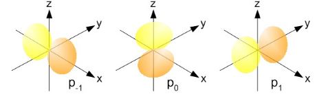 

In addition, you may also want to note the 45° angle we associate with m = ±1 does sort of demarcate the lobes of the distribution by defining a three-dimensional cone and… Well… I know these arguments are rather intuitive, and so you may refuse to accept them. In fact, to some extent, I refuse to accept them. 🙂 Indeed, let me say this loud and clear: I really want to understand this in a better way! 

But… Then… Well… Such better understanding may never come. Feynman’s warning, just before he starts explaining the Stern-Gerlach experiment and the quantization of angular momentum, rings very true here: “Understanding of these matters comes very slowly, if at all. Of course, one does get better able to know what is going to happen in a quantum-mechanical situation—if that is what understanding means—but one never gets a comfortable feeling that these quantum-mechanical rules are “natural.” Of course they are, but they are not natural to our own experience at an ordinary level.” So… Well… What can I say?

It is now time to pull the rabbit out of the hat. To understand what we’re going to do next, you need to remember that our amplitudes – or wavefunctions – are always expressed with regard to a specific frame of reference, i.e. some specific choice of an x-, y– and z-axis. If we change the reference frame – say, to some new set of x’-, y’– and z’-axes – then we need to re-write our amplitudes (or wavefunctions) in terms of the new reference frame. In order to do so, one should use a set of transformation rules. I’ve written several posts on that – including a very basic one, which you may want to re-read (just click the link here).

Look at the illustration below. We want to calculate the amplitude to find the electron at some point in space. Our reference frame is the x, y, z frame and the polar coordinates (or spherical coordinates, I should say) of our point are the radial distance r, the polar angle θ (theta), and the azimuthal angle φ (phi). [The illustration below – which I copied from Feynman’s exposé – uses a capital letter for phi, but I stick to the more usual or more modern convention here.]

In case you wonder why we’d use polar coordinates rather than Cartesian coordinates… Well… I need to refer you to my other post on the topic of electron orbitals, i.e. the one in which I explain how we get the spherically symmetric solutions: if you have radial (central) fields, then it’s easier to solve stuff using polar coordinates – although you wouldn’t think so if you think of that monster equation that we’re actually trying to solve here:

It’s really Schrödinger’s equation for the situation on hand (i.e. a hydrogen atom, with a radial or central Coulomb field because of its positively charged nucleus), but re-written in terms of polar coordinates. For the detail, see the mentioned post. Here, you should just remember we got the spherically symmetric solutions assuming the derivatives of the wavefunction with respect to θ and φ – so that’s the ∂ψ/∂θ and ∂ψ/∂φ in the equation above – were zero. So now we don’t assume these partial derivatives to be zero: we’re looking for states with an angular dependence, as Feynman puts it somewhat enigmatically. […] Yes. I know. This post is becoming very long, and so you are getting impatient. Look at the illustration with the (r, θ, φ) point, and let me quote Feynman on the line of reasoning now:

“Suppose we have the atom in some |l, m〉 state, what is the amplitude to find the electron at the angles θ and φ and the distance r from the origin? Put a new z-axis, say z’, at that angle (see the illustration above), and ask: what is the amplitude that the electron will be at the distance r along the new z’-axis? We know that it cannot be found along z’ unless its z’-component of angular momentum, say m’, is zero. When m’ is zero, however, the amplitude to find the electron along z’ is F_l(r). Therefore, the result is the product of two factors. The first is the amplitude that an atom in the state |l, m〉 along the z-axis will be in the state |l, m’ = 0〉 with respect to the z’-axis. Multiply that amplitude by F_l(r) and you have the amplitude ψ_l,m(r) to find the electron at (r, θ, φ) with respect to the original axes.”

So what is he telling us here? Well… He’s going a bit fast here. 🙂 Worse, I think he may actually not have chosen the right words here, so let me try to rephrase it. We’ve introduced the F_l(r) function above: it was the amplitude, for m = 0, to find the electron on the z-axis at some distance r. But so here we’re obviously in the x’, y’, z’ frame and so F_l(r) is the amplitude for m’ = 0,  it’s the amplitude to find the electron on the z-axis at some distance r along the z’-axis. Of course, for this amplitude to be non-zero, we must be in the |l, m’ = 0〉 state, but are we? Well… |l, m’ = 0〉 actually gives us the amplitude for that. So we’re going to multiply two amplitudes here:

F_l(r)·|l, m’ = 0〉

So this amplitude is the product of two amplitudes as measured in the the x’, y’, z’ frame. Note it’s symmetric: we may also write it as |l, m’ = 0〉·F_l(r). We now need to sort of translate that into an amplitude as measured in the x, y, z frame. To go from x, y, z to x’, y’, z’, we first rotated around the z-axis by the angle φ, and then rotated around the new y’-axis by the angle θ. Now, the order of rotation matters: you can easily check that by taking a non-symmetrical object in your hand and doing those rotations in the two different sequences: check what happens to the orientation of your object. Hence, to go back we should first rotate about the y’-axis by the angle −θ, so our z’-axis folds into the old z-axis, and then rotate about the z-axis by the angle −φ.

Now, we will denote the transformation matrices that correspond to these rotations as R_y’(−θ) and R_z(−φ) respectively. These transformation matrices are complicated beasts. They are surely not the easy rotation matrices that you can use for the coordinates themselves. You can click this link to see how they look like for l = 1. For larger l, there are other formulas, which Feynman derives in another chapter of his Lectures on quantum mechanics. But let’s move on. Here’s the grand result:

The amplitude for our wavefunction ψ_l,m(r) – which denotes the amplitude for (1) the atom to be in the state that’s characterized by the quantum numbers l and m and – let’s not forget – (2) find the electron at r – note the bold type: r = (x, y, z) – would be equal to:

ψ_l,m(r) = 〈l, m|R_z(−φ) R_y’(−θ)|l, m’ = 0〉·F_l(r)

Well… Hmm… Maybe. […] That’s not how Feynman writes it. He writes it as follows:

ψ_l,m(r) = 〈l, 0|R_y(θ) R_z(φ)|l, m〉·F_l(r)

I am not quite sure what I did wrong. Perhaps the two expressions are equivalent. Or perhaps – is it possible at all? – Feynman made a mistake? I’ll find out. [P.S: I re-visited this point in the meanwhile: see the P.S. to this post. :-)] The point to note is that we have some combined rotation matrix R_y(θ) R_z(φ). The elements of this matrix are algebraic functions of θ and φ, which we will write as Y_l,m(θ, φ), so we write:

a·Y_l,m(θ, φ) = 〈l, 0|R_y(θ) R_z(φ)|l, m〉

Or a·Y_l,m(θ, φ) = 〈l, m|R_z(−φ) R_y’(−θ)|l, m’ = 0〉, if Feynman would have it wrong and my line of reasoning above would be correct – which is obviously not so likely. Hence, the ψ_l,m(r) function is now written as:

ψ_l,m(r) = a·Y_l,m(θ, φ)·F_l(r)

The coefficient a is, as usual, a normalization coefficient so as to make sure the surface under the probability density function is 1. As mentioned above, we get these Y_l,m(θ, φ) functions from combining those rotation matrices. For l = 1, and m = -1, 0, +1, they are: A more complete table is given below: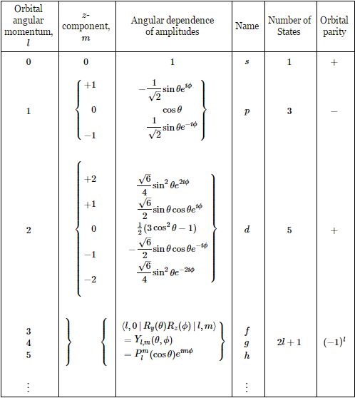So, yes, we’re done. Those equations above give us those wonderful shapes for the electron orbitals, as illustrated below (credit for the illustration goes to an interesting site of the UC Davis school).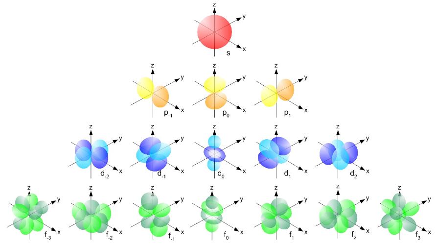But… Hey! Wait a moment! We only have these Y_l,m(θ, φ) functions here. What about F_l(r)?

You’re right. We’re not quite there yet, because we don’t have a functional form for F_l(r). Not yet, that is. Unfortunately, that derivation is another lengthy development – and that derivation actually is just tedious math only. Hence, I will refer you to Feynman for that. 🙂 Let me just insert one more thing before giving you The Grand Equation, and that’s a explanation of how we get those nice graphs. They are so-called polar graphs. There is a nice and easy article on them on the website of the University of Illinois, but I’ll summarize it for you. Polar graphs use a polar coordinate grid, as opposed to the Cartesian (or rectangular) coordinate grid that we’re used to. It’s shown below.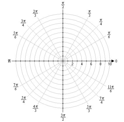 

The origin is now referred to as the pole – like in North or South Pole indeed. 🙂 The straight lines from the pole (like the diagonals, for example, or the axes themselves, or any line in-between) measure the distance from the pole which, in this case, goes from 0 to 10, and we can connect the equidistant points by a series of circles – as shown in the illustration also. These lines from the pole are defined by some angle – which we’ll write as θ to make things easy 🙂 – which just goes from 0 to 2π = 0 and then round and round and round again. The rest is simple: you’re just going to graph a function, or an equation – just like you’d graph y = ax + b in the Cartesian plane – but it’s going to be a polar equation. Referring back to our p-orbitals, we’ll want to graph the cos²θ = ρ equation, for example, because that’s going to show us the shape of that probability density function for l = 1 and m = 0. So our graph is going to connect the (θ, ρ) points for which the angle (θ) and the distance from the pole (ρ) satisfies the cos²θ = ρ equation. There is a really nice widget on the WolframAlpha site that produces those graphs for you. I used it to produce the graph below, which shows the 1.1547·cos²θ = ρ graph (the 1.1547 coefficient is the normalization coefficient a). 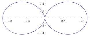Now, you’ll wonder why this is a curve, or a curved line. That widget even calculates its length: it’s about 6.374743 units long. So why don’t we have a surface or a volume here? We didn’t specify any value for ρ, did we? No, we didn’t. The widget calculates those values from the equation. So… Yes. It’s a valid question: where’s the distribution? We were talking about some electron cloud or something, right?

Right. To get that cloud – those probability densities really – we need that F_l(r) function. Our cos²θ = ρ is, once again, just some kind of envelope function: it marks a space but doesn’t fill it, so to speak. 🙂 In fact, I should now give you the complete description, which has all of the possible states of the hydrogen atom – everything! No separate pieces anymore. Here it is. It also includes n. It’s The Grand Equation: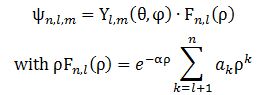The a_k coefficients in the formula for ρF_n,l(ρ) are the solutions to the equation below, which I copied from Feynman’s text on it all. I’ll also refer you to the same text to see how you actually get solutions out of it, and what they then actually represent. 🙂We’re done. Finally!

I hope you enjoyed this. Look at what we’ve achieved. We had this differential equation (a simple diffusion equation, really, albeit in the complex space), and then we have a central Coulomb field and the rather simple concept of quantized (i.e. non-continuous or discrete) angular momentum. Now see what magic comes out of it! We literally constructed the atomic structure out of it, and it’s all wonderfully elegant and beautiful.

Now I think that’s amazing, and if you’re reading this, then I am sure you’ll find it as amazing as I do.

Note: I did a better job in explaining the intricacies of actually representing those orbitals in a later post. I recommend you have a look at it by clicking the link here.

Post scriptum on the transformation matrices:

You must find the explanation for that 〈l, 0|R_y(θ) R_z(φ)|l, m〉·F_l(r) product highly unsatisfactory, and it is. 🙂 I just wanted to make you think – rather than just superficially read through it. First note that F_l(r)·|l, m’ = 0〉 is not a product of two amplitudes: it is the product of an amplitude with a state. A state is a vector in a rather special vector space – a Hilbert space (just a nice word to throw around, isn’t it?). The point is: a state vector is written as some linear combination of base states. Something inside of me tells me we may look at the three p-states as base states, but I need to look into that.

Let’s first calculate the R_y(θ) R_z matrix to see if we get those formulas for the angular dependence of the amplitudes. It’s the product of the R_y(θ) and R_z matrices, which I reproduce below.

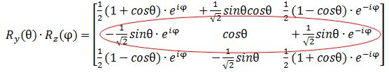Note that this product is non-commutative because… Well… Matrix products generally are non-commutative. 🙂 So… Well… There they are: the second row gives us those functions, so I am wrong, obviously, and Dr. Feynman is right. Of course, he is. He is always right – especially because his Lectures have gone through so many revised editions that all errors must be out by now. 🙂

However, let me – just for fun – also calculate my R_z(−φ) R_y’(−θ) product. I can do so in two steps: first I calculate R_z(φ) R_y’(θ), and then I substitute the angles φ and θ for –φ and –θ, remembering that cos(–α) = cos(α) and sin(–α) = –sin(α). I might have made a mistake, but I got this: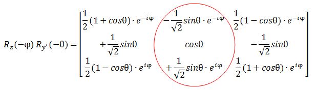The functions look the same but… Well… No. The e^iφ and e^−iφ are in the wrong place (it’s just one minus sign – but it’s crucially different). And then these functions should not be in a column. That doesn’t make sense when you write it all out. So Feynman’s expression is, of course, fully correct. But so how do we interpret that 〈l, 0|R_y(θ) R_z(φ)|l, m〉 expression then? This amplitude probably answers the following question:

Given that our atom is in the |l, m〉 state, what is the amplitude for it to be in the 〈l, 0| state in the x’, y’, z’ frame?

That makes sense – because we did start out with the assumption that our atom was in the the |l, m〉 state, so… Yes. Think about it some more and you’ll see it all makes sense: we can – and should – multiply this amplitude with the F_l(r) amplitude.

OK. Now we’re really done with this. 🙂

Note: As for the 〈 | and  | 〉 symbols to denote a state, note that there’s not much difference: both are state vectors, but a state vector that’s written as an end state – so that’s like 〈 Φ | – is a 1×3 vector (so that’s a column vector), while a vector written as | Φ 〉 is a 3×1 vector (so that’s a row vector). So that’s why 〈l, 0|R_y(θ) R_z(φ)|l, m〉 does give us some number. We’ve got a (1×3)·(3×3)·(3×1) matrix product here – but so it gives us what we want: a 1×1 amplitude. 🙂

Some content on this page was disabled on June 16, 2020 as a result of a DMCA takedown notice from The California Institute of Technology. You can learn more about the DMCA here:

https://en.support.wordpress.com/copyright-and-the-dmca/
Some content on this page was disabled on June 16, 2020 as a result of a DMCA takedown notice from The California Institute of Technology. You can learn more about the DMCA here:

https://en.support.wordpress.com/copyright-and-the-dmca/
Some content on this page was disabled on June 16, 2020 as a result of a DMCA takedown notice from The California Institute of Technology. You can learn more about the DMCA here:

https://en.support.wordpress.com/copyright-and-the-dmca/
Some content on this page was disabled on June 16, 2020 as a result of a DMCA takedown notice from The California Institute of Technology. You can learn more about the DMCA here:

https://en.support.wordpress.com/copyright-and-the-dmca/
Some content on this page was disabled on June 17, 2020 as a result of a DMCA takedown notice from Michael A. Gottlieb, Rudolf Pfeiffer, and The California Institute of Technology. You can learn more about the DMCA here:

https://en.support.wordpress.com/copyright-and-the-dmca/
Some content on this page was disabled on June 17, 2020 as a result of a DMCA takedown notice from Michael A. Gottlieb, Rudolf Pfeiffer, and The California Institute of Technology. You can learn more about the DMCA here:

https://en.support.wordpress.com/copyright-and-the-dmca/