Re-visiting electron orbitals (II)

Pre-script (dated 26 June 2020): Our ideas have evolved into a full-blown realistic (or classical) interpretation of all things quantum-mechanical. In addition, I note the dark force has amused himself by removing some material. So no use to read this. Read my recent papers instead. 🙂

Original post:

I’ve talked about electron orbitals in a couple of posts already – including a fairly recent one, which is why I put the (II) after the title. However, I just wanted to tie up some loose ends here – and do some more thinking about the concept of a definite energy state. What is it really? We know the wavefunction for a definite energy state can always be written as:

ψ(x, t) = e^{−i·(E/ħ)·t}·ψ(x)

Well… In fact, we should probably formally prove that but… Well… Let us just explore this formula in a more intuitive way – for the time being, that is – using those electron orbitals we’ve derived.

First, let me note that ψ(x, t) and ψ(x) are very different functions and, therefore, the choice of the same symbol for both (the Greek psi) is – in my humble opinion – not very fortunate, but then… Well… It is the choice of physicists – as copied in textbooks all over – and so we’ll just have to live with it. Of course, we can appreciate why they choose to use the same symbol – ψ(x) is like a time-independent wavefunction now, so that’s nice – but… Well… You should note that it is not so obvious to write some function as the product of two other functions. To be complete, I’ll be a bit more explicit here: if some function in two variables – say F(x, y) – can be written as the product of two functions in one variable – say f(x) and g(y), so we can write F as F(x, y) = f(x)·g(y) – then we say F is a separable function. For a full overview of what that means, click on this link. And note mathematicians do choose a different symbol for the functions F and g. It would probably be interesting to explore what the conditions for separability actually imply in terms of properties of… Well… The wavefunction and its argument, i.e. the space and time variables. But… Well… That’s stuff for another post. 🙂

Secondly, note that the momentum variable (p) – i.e. the p in our elementary wavefunction a·e^{i·(p·x−E·t)/ħ} has sort of vanished: ψ(x) is a function of the position only. Now, you may think it should be somewhere there – that, perhaps, we can write something like ψ(x) = ψ[x), p(x)]. But… No. The momentum variable has effectively vanished. Look at Feynman’s solutions for the electron orbitals of a hydrogen atom: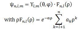The Y_l,m(θ, φ) and F_n,l(ρ) functions here are functions of the (polar) coordinates ρ, θ, φ only. So that’s the position only (these coordinates are polar or spherical coordinates, so ρ is the radial distance, θ is the polar angle, and φ is the azimuthal angle). There’s no idea whatsoever of any momentum in one or the other spatial direction here. I find that rather remarkable. Let’s see how it all works with a simple example.

The functions below are the Y_l,m(θ, φ) for l = 1. Note the symmetry: if we swap θ and φ for -θ and -φ respectively, we get the other function: 2^-1/2·sin(-θ)·e^–i(-φ) = -2^-1/2·sinθ·e^iφ.

To get the probabilities, we need to take the absolute square of the whole thing, including e^−i·(E/ħ), but we know |e^i·δ|² = 1 for any value of δ. Why? Because the absolute square of any complex number is the product of the number with its complex conjugate, so |e^i·δ|² = e^i·δ·e^–i·δ = e^i·0 = 1. So we only have to look at the absolute square of the Y_l,m(θ, φ) and F_n,l(ρ) functions here. The F_n,l(ρ) function is a real-valued function, so its absolute square is just what it is: some real number (I gave you the formula for the a_k coefficients in my post on it, and you shouldn’t worry about them: they’re real too). In contrast, the Y_l,m(θ, φ) functions are complex-valued – most of them are, at least. Unsurprisingly, we find the probabilities are also symmetric:

P = |-2^-1/2·sinθ·e^iφ|² = (-2^-1/2·sinθ·e^iφ)·(-2^-1/2·sinθ·e^–iφ)

= (2^-1/2·sinθ·e^–iφ)·(2^-1/2·sinθ·e^iφ) =  |2^-1/2·sinθ·e^–iφ|² = (1/2)·sin²θ

Of course, for m = 0, the probability is just cos²θ. The graphs below are the polar graphs for the cos²θ and (1/2)·sin²θ functions respectively.

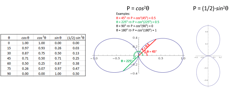These polar graphs are not so easy to interpret, so let me say a few words about them. The points that are plotted combine (a) some radial distance from the center – which I wrote as P because this distance is, effectively, a probability – with (b) the polar angle θ (so that’s one of the  three coordinates). To be precise, the plot gives us, for a given ρ, all of the (θ, P) combinations. It works as follows. To calculate the probability for some ρ and θ (note that φ can be any angle), we must take the absolute square of that ψ_n,l,m, = Y_l,m(θ, φ)·F_n,l(ρ) product. Hence, we must calculate |Y_l,m(θ, φ)·F_n,l(ρ)|² = |F_n,l(ρ)|²·cos²θ for m = 0, and (1/2)·|F_n,l(ρ)|²·sin²θ for m = ±1. Hence, the value of ρ determines the value of F_n,l(ρ), and that F_n,l(ρ) value then determines the shape of the polar graph. The three graphs below – P = cos²θ, P = (1/2)·cos²θ and P = (1/4)·cos²θ – illustrate the idea. Note that we’re measuring θ from the z-axis here, as we should. So that gives us the right orientation of this volume, as opposed to the other polar graphs above, which measured θ from the x-axis. So… Well… We’re getting there, aren’t we? 🙂

Now you’ll have two or three – or even more – obvious questions. The first one is: where is the third lobe? That’s a good question. Most illustrations will represent the p-orbitals as follows: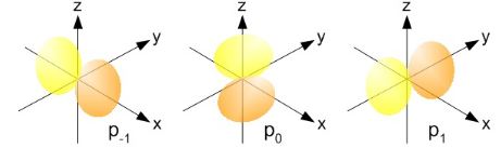Three lobes. Well… Frankly, I am not quite sure here, but the equations speak for themselves: the probabilities only depend on ρ and θ. Hence, the azimuthal angle φ can be anything. So you just need to rotate those P = (1/2)·sin²θ and P = cos²θ curves about the the z-axis. In case you wonder how to do that, the illustration below may inspire you.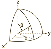The second obvious question is about the size of those lobes. That 1/2 factor must surely matter, right? Well… We still have that F_n,l(ρ) factor, of course, but you’re right: that factor does not depend on the value for m: it’s the same for m = 0 or ± 1. So… Well… Those representations above – with the three lobes, all of the same volume – may not be accurate. I found an interesting site – Atom in a Box – with an app that visualizes the atomic orbitals in a fun and exciting way. Unfortunately, it’s for Mac and iPhone only – but this YouTube video shows how it works. I encourage you to explore it. In fact, I need to explore it – but what I’ve seen on that YouTube video (I don’t have a Mac nor an iPhone) suggests the three-lobe illustrations may effectively be wrong: there’s some asymmetry here – which we’d expect, because those p-orbitals are actually supposed to be asymmetric! In fact, the most accurate pictures may well be the ones below. I took them from Wikimedia Commons. The author explains the use of the color codes as follows: “The depicted rigid body is where the probability density exceeds a certain value. The color shows the complex phase of the wavefunction, where blue means real positive, red means imaginary positive, yellow means real negative and green means imaginary negative.” I must assume he refers to the sign of a and b when writing a complex number as a + i·b

The third obvious question is related to the one above: we should get some cloud, right? Not some rigid body or some surface. Well… I think you can answer that question yourself now, based on what the author of the illustration above wrote: if we change the cut-off value for the probability, then we’ll give a different shape. So you can play with that and, yes, it’s some cloud, and that’s what the mentioned app visualizes. 🙂

The fourth question is the most obvious of all. It’s the question I started this post with: what are those definite energy states? We have uncertainty, right? So how does that play out? Now that is a question I’ll try to tackle in my next post. Stay tuned ! 🙂

Post scriptum: Let me add a few remarks here so as to – hopefully – contribute to an even better interpretation of what’s going on here. As mentioned, the key to understanding is, obviously, the following basic functional form:

ψ(r, t) = e^{−i·(E/ħ)·t}·ψ(r)

Wikipedia refers to the e^{−i·(E/ħ)·t} factor as a time-dependent phase factor which, as you can see, we can separate out because we are looking at a definite energy state here. Note the minus sign in the exponent – which reminds us of the minus sign in the exponent of the elementary  wavefunction, which we wrote as:

 a·e^−i·θ = a·e^{−i·[(E/ħ)·t − (p/ħ)∙x]} = a·e^{i·[(p/ħ)∙x − (E/ħ)·t]} = a·e^{−i·(E/ħ)·t}·e^{i·(p/ħ)∙x}

We know this elementary wavefunction is problematic in terms of interpretation because its absolute square gives us some constant probability P(x, t) = |a·e^{−i·[(E/ħ)·t − (p/ħ)∙x]}|² = a². In other words, at any point in time, our electron is equally likely to be anywhere in space. That is not consistent with the idea of our electron being somewhere at some point in time.

The other question is: what reference frame do we use to measure E and p? Indeed, the value of E and p = (p_x, p_y, p_z) depends on our reference frame: from the electron’s own point of view, it has no momentum whatsoever: p = 0. Fortunately, we do have a point of reference here: the nucleus of our hydrogen atom. And our own position, of course, because you should note, indeed, that both the subject and the object of the observation are necessary to define the Cartesian x = x, y, z – or, more relevant in this context – the polar r = ρ, θ, φ coordinates.

This, then, defines some finite or infinite box in space in which the (linear) momentum (p) of our electron vanishes, and then we just need to solve Schrödinger’s diffusion equation to find the solutions for ψ(r). These solutions are more conveniently written in terms of the radial distance ρ, the polar angle θ, and the azimuthal angle φ:

The functions below are the Y_l,m(θ, φ) functions for l = 1.

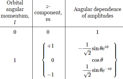
The interesting thing about these Y_l,m(θ, φ) functions is the e^i·φ and/or e^−i·φ factor. Indeed, note the following:

1. Because the sinθ and cosθ factors are real-valued, they only define some envelope for the ψ(r) function.
2. In contrast, the e^i·φ and/or e^−i·φ factor define some phase shift.

Let’s have a look at the physicality of the situation, which is depicted below.

The nucleus of our hydrogen atom is at the center. The polar angle is measured from the z-axis, and we know we only have an amplitude there for m = 0, so let’s look at what that cosθ factor does. If θ = 0°, the amplitude is just what it is, but when θ > 0°, then |cosθ| < 1 and, therefore, the probability P = |F_n,l(ρ)|²·cos²θ will diminish. Hence, for the same radial distance (ρ), we are less likely to find the electron at some angle θ > 0° than on the z-axis itself. Now that makes sense, obviously. You can work out the argument for m = ± 1 yourself, I hope. [The axis of symmetry will be different, obviously!] 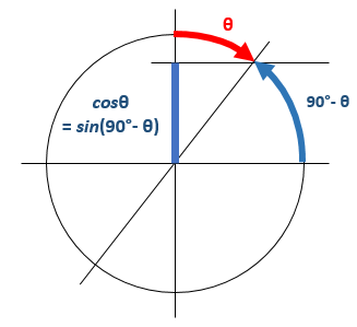In contrast, the e^i·φ and/or e^−i·φ factor work very differently. These just give us a phase shift, as illustrated below. A re-set of our zero point for measuring time, so to speak, and the e^i·φ and/or e^−i·φ factor effectively disappears when we’re calculating probabilities, which is consistent with the fact that this angle clearly doesn’t influence the magnitude of the amplitude fluctuations.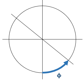So… Well… That’s it, really. I hope you enjoyed this ! 🙂

Some content on this page was disabled on June 16, 2020 as a result of a DMCA takedown notice from The California Institute of Technology. You can learn more about the DMCA here:

https://en.support.wordpress.com/copyright-and-the-dmca/