Pre-scriptum (dated 26 June 2020): These posts on elementary math and physics have not suffered much the attack by the dark force—which is good because I still like them. While my views on the true nature of light, matter and the force or forces that act on them have evolved significantly as part of my explorations of a more realist (classical) explanation of quantum mechanics, I think most (if not all) of the analysis in this post remains valid and fun to read. In fact, I find the simplest stuff is often the best. 🙂
Original post:
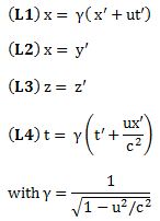
This is my third and final post about special relativity. In the previous posts, I introduced the general idea and the Lorentz transformations. I present these Lorentz transformations once again below, next to their Galilean counterparts. [Note that I continue to assume, for simplicity, that the two reference frames move with respect to each other along the x- axis only, so the y- and z-component of u is zero. It is not all that difficult to generalize to three dimensions (especially not when using vectors) but it makes an intuitive understanding of what’s relativity all about more difficult.]
 As you can see, under a Lorentz transformation, the new ‘primed’ space and time coordinates are a mixture of the ‘unprimed’ ones. Indeed, the new x’ is a mixture of x and t, and the new t’ is a mixture as well. You don’t have that under a Galilean transformation: in the Newtonian world, space and time are neatly separated, and time is absolute, i.e. it is the same regardless of the reference frame. In Einstein’s world – our world – that’s not the case: time is relative, or local as Hendrik Lorentz termed it, and so it’s space-time – i.e. ‘some kind of union of space and time’ as Minkowski termed it – that transforms. In practice, physicists will use so-called four-vectors, i.e. vectors with four coordinates, to keep track of things. These four-vectors incorporate both the three-dimensional space vector as well as the time dimension. However, we won’t go into the mathematical details of that here.
What else is relative? Everything, except the speed of light. Of course, velocity is relative, just like in the Newtonian world, but the equation to go from a velocity as measured in one reference frame to a velocity as measured in the other, is different: it’s not a matter of just adding or subtracting speeds. In addition, besides time, mass becomes a relative concept as well in Einstein’s world, and that was definitely not the case in the Newtonian world.
What about energy? Well… We mentioned that velocities are relative in the Newtonian world as well, so momentum and kinetic energy were relative in that world as well: what you would measure for those two quantities would depend on your reference frame as well. However, here also, we get a different formula now. In addition, we have this weird equivalence between mass and energy in Einstein’s world, about which I should also say something more.
But let’s tackle these topics one by one. We’ll start with velocities.
Relativistic velocity
In the Newtonian world, it was easy. From the Galilean transformation equations above, it’s easy to see that
v’ = dx’/dt’ = d(x – ut)/dt = dx/dt – d(ut)/dt = v – u
So, in the Newtonian world, it’s just a matter of adding/subtracting speeds indeed: if my car goes 100 km/h (v), and yours goes 120 km/h, then you will see my car falling behind at a speed of (minus) 20 km/h. That’s it. In Einstein’s world, it is not so simply. Let’s take the spaceship example once again. So we have a man on the ground (the inertial or ‘unprimed’ reference frame) and a man in the spaceship (the primed reference frame), which is moving away from us with velocity u.
Now, suppose an object is moving inside the spaceship (along the x-axis as well) with a (uniform) velocity vx’, as measured from the point of view of the man inside the spaceship. Then the displacement x’ will be equal to x’ = vx’ t’. To know how that looks from the man on the ground, we just need to use the opposite Lorentz transformations: just replace u by –u everywhere (to the man in the spaceship, it’s like the man on the ground moves away with velocity –u), and note that the Lorentz factor does not change because we’re squaring and (–u)2 = u2. So we get:
Hence, x’ = vx’ t’ can be written as x = γ(vx’ t’ + ut’). Now we should also substitute t’, because we want to measure everything from the point of view of the man on the ground. Now, t = γ(t’ + uvx’ t’/c2). Because we’re talking uniform velocities, vx (i.e. the velocity of the object as measured by the man on the ground) will be equal to x divided by t (so we don’t need to take the time derivative of x), and then, after some simplifying and re-arranging (note, for instance, how the t’ factor miraculously disappears), we get:
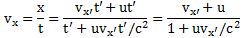
What does this rather complicated formula say? Just put in some numbers:
- Suppose the object is moving at half the speed of light, so 0.5c, and that the spaceship is moving itself also at 0.5c, then we get the rather remarkable result that, from the point of view of the observer on the ground, that object is not going as fast as light, but only at vx = (0.5c + 0.5c)/(1 + 0.5·0.5) = 0.8c.
- Or suppose we’re looking at a light beam inside the spaceship, so something that’s traveling at speed c itself in the spaceship. How does that look to the man on the ground? Just put in the numbers: vx = (0.5c + c)/(1 + 0.5·1) = c ! So the speed of light is not dependent on the reference frame: it looks the same – both to the man in the ship as well as to the man on the ground. As Feynman puts it: “This is good, for it is, in fact, what the Einstein theory of relativity was designed to do in the first place–so it had better work!”
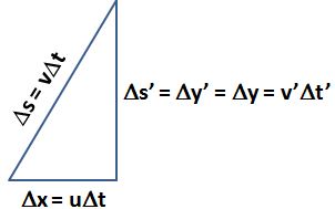
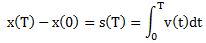
It’s interesting to note that, even if u has no y– or z-component, velocity in the y direction will be affected too. Indeed, if an object is moving upward in the spaceship, then the distance of travel of that object to the man on the ground will appear to be larger. See the triangle below: if that object travels a distance Δs’ = Δy’ = Δy = v’Δt’ with respect to the man in the spaceship, then it will have traveled a distance Δs = vΔt to the man on the ground, and that distance is longer.
 I won’t go through the process of substituting and combining the Lorentz equations (you can do that yourself) but the grand result is the following:
vy = (1/γ)vy’
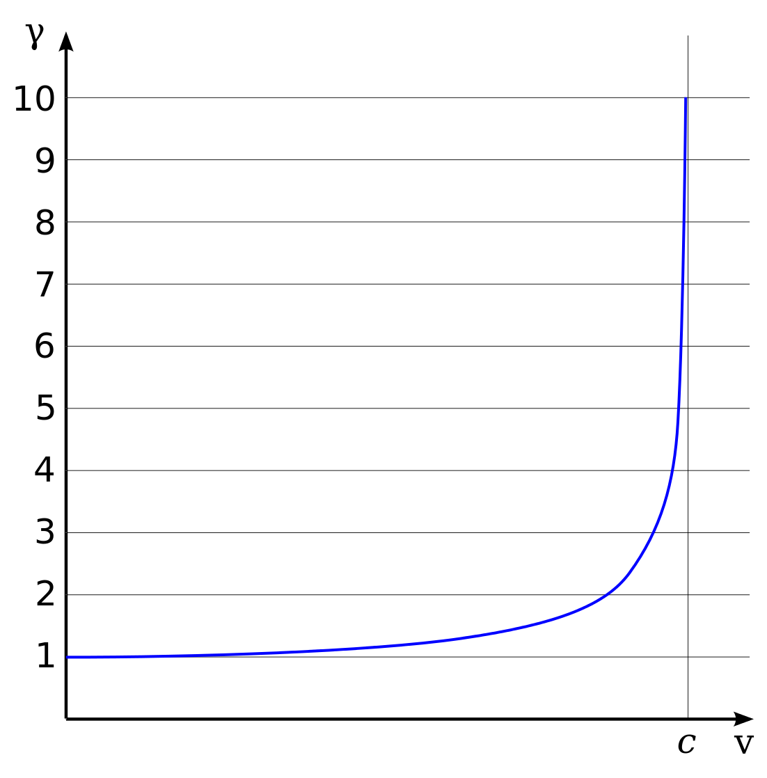
1/γ is the reciprocal of the Lorentz factor, and I’ll leave it to you to work out a few numeric examples. When you do that, you’ll find the rather remarkable result that vy is actually less than vy’. For example, for u = 0.6c, 1/γ will be equal to 0.8, so vy will be 20% less than vy’. How is that possible? The vertical distance is what it is (Δy’ = Δy), and that distance is not affected by the ‘length contraction’ effect (y’ = y). So how can the vertical velocity be smaller? The answer is easy to state, but not so easy to understand: it’s the time dilation effect: time in the spaceship goes slower. Hence, the object will cover the same vertical distance indeed – for both observers – but, from the point of view of the observer on the ground, the object will apparently need more time to cover that distance than the time measured by the man in the spaceship: Δt > Δt’. Hence, the logical conclusion is that the vertical velocity of that object will appear to be less to the observer on the ground.
How much less? The time dilation factor is the Lorentz factor. Hence, Δt = γΔt’. Now, if u = 0.6c, then γ will be equal to 1.25 and Δt = 1.25Δt’. Hence, if that object would need, say, one second to cover that vertical distance, then, from the point of view of the observer on the ground, it would need 1.25 seconds to cover the same distance. Hence, its speed as observed from the ground is indeed only 1/(5/4) = 4/5 = 0.8 of its speed as observed by the man in the spaceship.
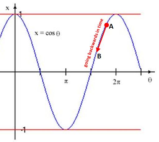
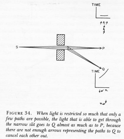
Is that hard to understand? Maybe. You have to think through it. One common mistake is that people think that length contraction and/or time dilation are, somehow, related to the fact that we are looking at things from a distance and that light needs time to reach us. Indeed, on the Web, you can find complicated calculations using the angle of view and/or the line of sight (and tons of trigonometric formulas) as, for example, shown in the drawing below. These have nothing to do with relativity theory and you’ll never get the Lorentz transformation out of them. They are plain nonsense: they are rooted in an inability of these youthful authors to go beyond Galilean relativity. Length contraction and/or time dilation are not some kind of visual trick or illusion. If you want to see how one can derive the Lorentz factor geometrically, you should look for a good description of the Michelson-Morley experiment in a good physics handbook such as, yes :-), Feynman’s Lectures.
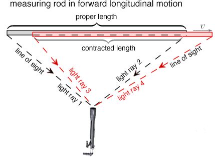
So, I repeat: illustrations that try to explain length contraction and time dilation in terms of line of sight and/or angle of view are useless and will not help you to understand relativity. On the contrary, they will only confuse you. I will let you think through this and move on to the next topic.
Relativistic mass and relativistic momentum
Einstein actually stated two principles in his (special) relativity theory:
- The first is the Principle of Relativity itself, which is basically just the same as Newton’s principle of relativity. So that was nothing new actually: “If a system of coordinates K is chosen such that, in relation to it, physical laws hold good in their simplest form, then the same laws must hold good in relation to any other system of coordinates K’ moving in uniform translation relatively to K.” Hence, Einstein did not change the principle of relativity – quite on the contrary: he re-confirmed it – but he did change Newton’s Laws, as well as the Galilean transformation equations that came with them. He also introduced a new ‘law’, which is stated in the second ‘principle’, and that the more revolutionary one really:
- The Principle of Invariant Light Speed: “Light is always propagated in empty space with a definite velocity [speed] c which is independent of the state of motion of the emitting body.”
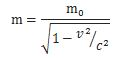
As mentioned above, the most notable change in Newton’s Laws – the only change, in fact – is Einstein’s relativistic formula for mass:
mv = γm0
This formula implies that the inertia of an object, i.e. its mass, also depends on the reference frame of the observer. If the object moves (but velocity is relative as we know: an object will not be moving if we move with it), then its mass increases. This affects its momentum. As you may or may not remember, the momentum of an object is the product of its mass and its velocity. It’s a vector quantity and, hence, momentum has not only a magnitude but also a direction:
pv = mvv = γm0v
As evidenced from the formula above, the momentum formula is a relativistic formula as well, as it’s dependent on the Lorentz factor too. So where do I want to go from here? Well… In this section (relativistic mass and momentum), I just want to show that Einstein’s mass formula is not some separate law or postulate: it just comes with the Lorentz transformation equations (and the above-mentioned consequences in terms of measuring horizontal and vertical velocities).
Indeed, Einstein’s relativistic mass formula can be derived from the momentum conservation principle, which is one of the ‘physical laws’ that Einstein refers to. Look at the elastic collision between two billiard balls below. These balls are equal – same mass and same speed from the point of view of an inertial observer – but not identical: one is red and one is blue. The two diagrams show the collision from two different points of view: left, we have the inertial reference frame, and, right, we have a reference frame that is moving with a velocity equal to the horizontal component of the velocity of the blue ball.

The points to note are the following:
- The total momentum of such elastic collision before and after the collision must be the same.
- Because the two balls have equal mass (in the inertial reference frame at least), the collision will be perfectly symmetrical. Indeed, we may just turn the diagram ‘upside down’ and change the colors of the balls, as we do below, and the values w, u and v (as well as the angle α) are the same.
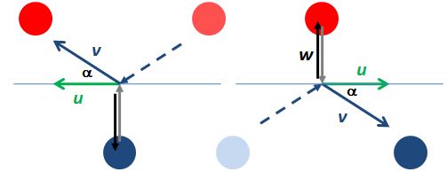
As mentioned above, the velocity of the blue and red ball and, hence, their momentum, will depend on the frame of reference. In the diagram on the left, we’re moving with a velocity equal to the horizontal component of the velocity of the blue ball and, therefore, in this particular frame of reference, the velocity (and the momentum) of the blue ball consists of a vertical component only, which we refer to as w.
From this point of view (i.e. the reference frame moving with, the velocity (and, hence, the momentum) of the red ball will have both a horizontal as well as a vertical component. If we denote the horizontal component by u, then it’s easy to show that the vertical velocity of the red ball must be equal to sin(α)v. Now, because u = cos(α)v, this vertical component will be equal to tan(α)u. But so what is tan(α)u? Now, you’ll say, that is quite evident: tan(α)u must be equal to w, right?
No. That’s Newtonian physics. The red ball is moving horizontally with speed u with respect to the blue ball and, hence, its vertical velocity will not be quite equal to w. Its vertical velocity will be given by the formula which we derived above: vy = (1/γ)vy’, so it will be a little bit slower than the w we see in the diagram on the right which is, of course, the same w as in the diagram on the left. [If you look carefully at my drawing above, then you’ll notice that the w vector is a bit longer indeed.]
Huh? Yes. Just think about it: tan(α)u = (1/γ)w. But then… How can momentum be conserved if these speeds are not the same? Isn’t the momentum conservation principle supposed to conserve both horizontal as well as vertical momentum? It is, and momentum is being conserved. Why? Because of the relativistic mass factor.
Indeed, the change in vertical momentum (Δp) of the blue ball in the diagram on the left or – which amounts to the same – the red ball in the diagram on the right (i.e. the vertically moving ball) is equal to Δpblue = 2mww. [The factor 2 is there because the ball goes down and then up (or vice versa) and, hence, the total change in momentum must be twice the mww amount.] Now, that amount must be equal to Δpred, which is equal to Δpblue = 2mv(1/γ)w. Equating both yields the following grand result:
mv/mw = γ ⇔ mv = γmw
What does this mean? It means that mass of the red ball in the diagram on the left is larger than the mass of the blue ball. So here we have actually derived Einstein’s relativistic mass formula from the momentum conservation principle !
Of course you’ll say: not quite. This formula is not the mu = γm0 formula that we’re used to ! Indeed, it’s not. The blue ball has some velocity w itself, and so the formula links two velocities v and w. However, we can derive mv = γm0 formula as a limit of mv = γmw for w going to zer0. How can w become infinitesimally small? If the angle α becomes infinitesimally small. It’s obvious, then, that v and u will be practically equal. In fact, if w goes to zero, then mw will be equal to m0 in the limiting case, and mv will be equal to mu. So, then, indeed, we get the familiar formula as a limiting case:
mu = γm0
Hmm… You’ll probably find all of this quite fishy. I’d suggest you just think about it. What I presented above, is actually Feynman’s presentation of the subject, but with a bit more verbosity. Let’s move on to the final.
Relativistic energy
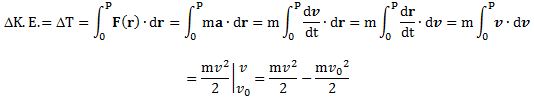
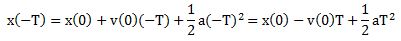
From what I wrote above (and from what I wrote in my two previous posts on this topic), it should be obvious, by now, that energy also depends on the reference frame. Indeed, mass and velocity depend on the reference frame (moving or not), and both appear in the formula for kinetic energy which, as you’ll remember, is
K.E. = mc2 – m0c2 = (m – m0)c2 = γm0c2 – m0c2 = m0c2(γ – 1).
Now, if you go back to the post where I presented that formula, you’ll see that we’re actually talking the change in kinetic energy here: if the mass is at rest, it’s kinetic energy is zero (because m = m0), and it’s only when the mass is moving, that we can observe the increase in mass. [If you wonder how, think about the example of the fast-moving electrons in an electron beam: we see it as an increase in the inertia: applying the same force does no longer yield the same acceleration.]
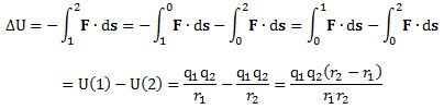
Now, in that same post, I also noted that Einstein added an equivalent rest mass energy (E0 = m0c2) to the kinetic energy above, to arrive at the total energy of an object:
E = E0 + K.E. = mc2
Now, what does this equivalence actually mean? Is mass energy? Can we equate them really? The short answer to that is: yes.
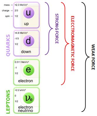
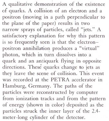
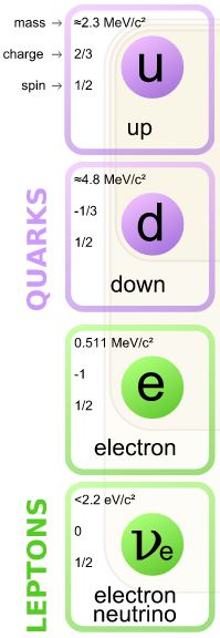
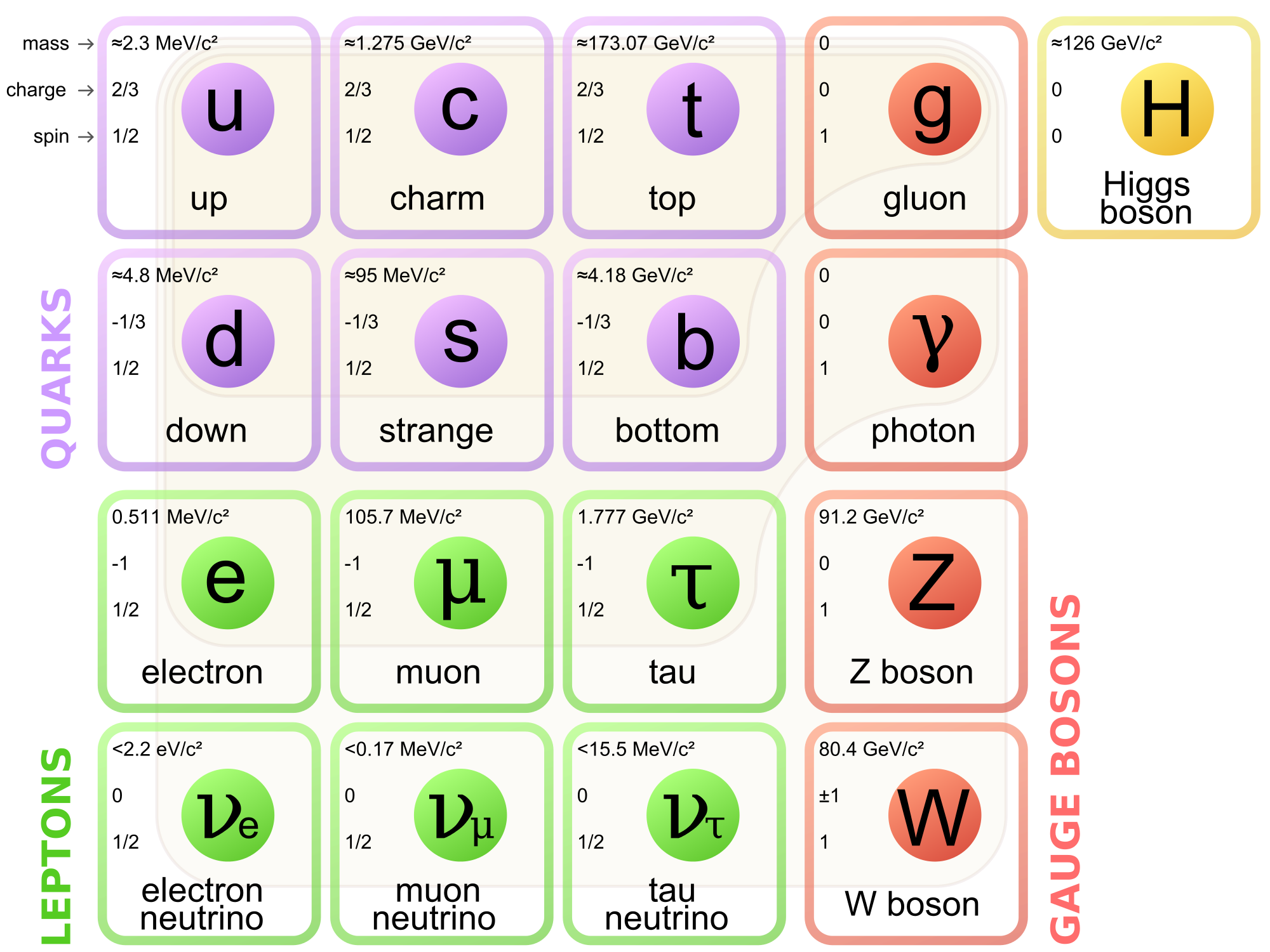
Indeed, in one of my older posts (Loose Ends), I explained that protons and neutrons are made of quarks and, hence, that quarks are the actual matter particles, not protons and neutrons. However, the mass of a proton – which consists of two up quarks and one down quark – is 938 MeV/c2 (don’t worry about the units I am using here: because protons are so tiny, we don’t measure their mass in grams), but the mass figure you get when you add the rest mass of two u‘s and one d, is 9.6 MeV/c2 only: about one percent of 938 ! So where’s the difference?
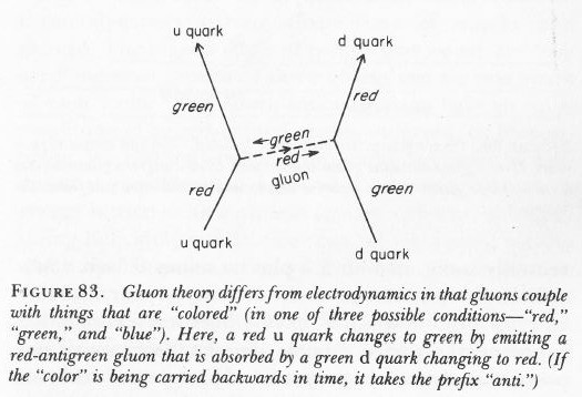
The difference is the equivalent mass (or inertia) of the binding energy between the quarks. Indeed, the so-called ‘mass’ that gets converted into energy when a nuclear bomb explodes is not the mass of quarks. Quarks survive: nuclear power is binding energy between quarks that gets converted into heat and radiation and kinetic energy and whatever else a nuclear explosion unleashes.
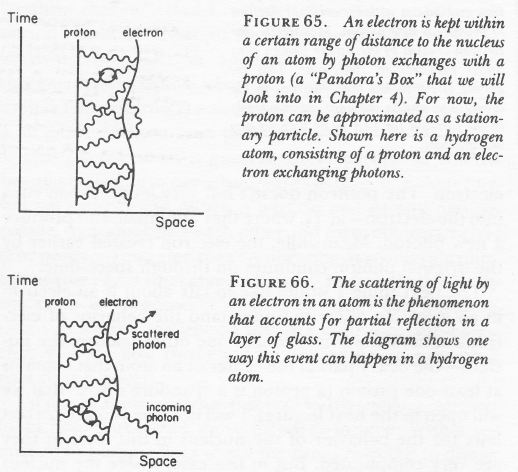
In short, 99% of the ‘mass’ of a proton or an electron is due to the strong force. So that’s ‘potential’ energy that gets unleashed in a nuclear chain reaction. In other words, the rest mass of the proton is actually the inertia of the system of moving quarks and gluons that make up the particle. In such atomic system, even the energy of massless particles (e.g. the virtual photons that are being exchanged between the nucleus and its electron shells) is measured as part of the rest mass of the system. So, yes, mass is energy. As Feynman put it, long before the quark model was confirmed and generally accepted:
“We do not have to know what things are made of inside; we cannot and need not justify, inside a particle, which of the energy is rest energy of the parts into which it is going to disintegrate. It is not convenient and often not possible to separate the total mc2 energy of an object into (1) rest energy of the inside pieces, (2) kinetic energy of the pieces, and (3) potential energy of the pieces; instead we simply speak of the total energy of the particle. We ‘shift the origin’ of energy by adding a constant m0c2 to everything, and say that the total energy of a particle is the mass in motion times c2, and when the object is standing still, the energy is the mass at rest times c2.” (Richard Feynman’s Lectures on Physics, Vol. I, p. 16-9)
So that says it all, I guess, and, hence, that concludes my little ‘series’ on (special) relativity. I hope you enjoyed it.
Post scriptum:
Feynman describes the concept of space-time with a nice analogy: “When we move to a new position, our brain immediately recalculates the true width and depth of an object from the ‘apparent’ width and depth. But our brain does not immediately recalculate coordinates and time when we move at high speed, because we have had no effective experience of going nearly as fast as light to appreciate the fact that time and space are also of the same nature. It is as though we were always stuck in the position of having to look at just the width of something, not being able to move our heads appreciably one way or the other; if we could, we understand now, we would see some of the other man’s time—we would see “behind”, so to speak, a little bit. Thus, we shall try to think of objects in a new kind of world, of space and time mixed together, in the same sense that the objects in our ordinary space-world are real, and can be looked at from different directions. We shall then consider that objects occupying space and lasting for a certain length of time occupy a kind of a “blob” in a new kind of world, and that when we look at this “blob” from different points of view when we are moving at different velocities. This new world, this geometrical entity in which the “blobs” exist by occupying position and taking up a certain amount of time, is called space-time.”
If none of what I wrote could convey the general idea, then I hope the above quote will. 🙂 Apart from that, I should also note that physicists will prefer to re-write the Lorentz transformation equations by measuring time and distance in so-called equivalent units: velocities will be expressed not in km/h but as a ratio of c and, hence, c = 1 (a pure number) and so u will also be a pure number between 0 and 1. That can be done by expressing distance in light-seconds ( a light-second is the distance traveled by light in one second or, alternatively, by expressing time in ‘meter’. Both are equivalent but, in most textbooks, it will be time that will be measured in the ‘new’ units. So how do we express time in meter?
It’s quite simple: we multiply the old seconds with c and then we get: timeexpressed in meters = timeexpressed in seconds multiplied by 3×10⁸ meters per second. Hence, as the ‘second’ the first factor and the ‘per second’ in the second factor cancel out, the dimension of the new time unit will effectively be the meter. Now, if both time and distance are expressed in meter, then velocity becomes a pure number without any dimension, because we are dividing distance expressed in meter by time expressed in meter, and it should be noted that it will be a pure number between 0 and 1 (0 ≤ u ≤ 1), because 1 ‘time second’ = 1/(3×108) ‘time meters’. Also, c itself becomes the pure number 1. The Lorentz transformation equations then become:
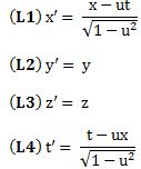
They are easy to remember in this form (cf. the symmetry between x – ut and t – ux) and, if needed, we can always convert back to the old units to recover the original formulas.
I personally think there is no better way to illustrate how space and time are ‘mere shadows’ of the same thing indeed: if we express both time and space in the same dimension (meter), we can see how, as result of that, velocity becomes a dimensionless number between zero and one and, more importantly, how the equations for x’ and t’ then mirror each other nicely. I am not sure what ‘kind of union’ between space and time Minkowski had in mind, but this must come pretty close, no?
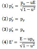
Final note: I noted the equivalence of mass and energy above. In fact, mass and energy can also be expressed in the same units, and we actually do that above already. If we say that an electron has a rest mass of 0.511 MeV/c2 (a bit less than a quarter of the mass of the u quark), then we express the mass in terms of energy. Indeed, the eV is an energy unit and so we’re actually using the m = E/c2 formula when we express mass in such units. Expressing mass and energy in equivalent units allows us to derive similar ‘Lorentz transformation equations’ for the energy and the momentum of an object as measured under an inertial versus a moving reference frame. Hence, energy and momentum also transform like our space-time four-vectors and – likewise – the energy and the momentum itself, i.e. the components of the (four-)vector, are less ‘real’ than the vector itself. However, I think this post has become way too long and, hence, I’ll just jot these four equations down – please note, once again, the nice symmetry between (1) and (2) – but then leave it at that and finish this post. 🙂


 As for the constants in this formula, you know these by now: the speed of light c, the electron charge e, its mass me, and the permittivity of free space εe. For whatever it’s worth (because you should note that, in quantum mechanics, electrons do not have a size: they are treated as point-like particles, so they have a point charge and zero dimension), that’s small. It’s in the femtometer range (1 fm = 1

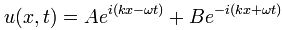

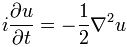

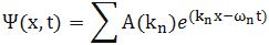
 Now if we plug that in the equation above, we get our time-dependent Schrödinger equation: