In my previous post,I introduced electric motors, generators and transformers. They all work because of Faraday’s flux rule: a changing magnetic flux will produce some circulation of the electric field. The formula for the flux rule is given below:

It is a wonderful thing, really, but not easy to grasp intuitively. It’s one of these equations where I should quote Feynman’s introduction to electromagnetism: “The laws of Newton were very simple to write down, but they had a lot of complicated consequences and it took us a long time to learn about them all. The laws of electromagnetism are not nearly as simple to write down, which means that the consequences are going to be more elaborate and it will take us quite a lot of time to figure them all out.”

Now, among Maxwell’s Laws, this is surely the most complicated one! However, that shouldn’t deter us. 🙂 Recalling Stokes’ Theorem helps to appreciate what the integral on the left-hand side represents:

We’ve got a line integral around some closed loop Γ on the left and, on the right, we’ve got a surface integral over some surface S whose boundary is Γ. The illustration below depicts the geometry of the situation. You know what it all means. If not, I am afraid I have to send you back to square one, i.e. my posts on vector analysis. Yep. Sorry. Can’t keep copying stuff and make my posts longer and longer. 🙂

To understand the flux rule, you should imagine that the loop Γ is some loop of electric wire, and then you just replace C by E, the electric field vector. The circulation of E, which is caused by the change in magnetic flux, is referred to as the electromotive force (emf), and it’s the tangential force (E·ds) per unit charge in the wire integrated over its entire length around the loop, which is denoted by Γ here, and which encloses a surface S.

Now, you can go from the line integral to the surface integral by noting Maxwell’s Law: −∂B/∂t = ∇×E. In fact, it’s the same flux rule really, but in differential form. As for (∇×E)_n, i.e. the component of ∇×E that is normal to the surface, you know that any vector multiplied with the normal unit vector will yield its normal component. In any case, if you’re reading this, you should already be acquainted with all of this. Let’s explore the concept of the electromotive force, and then apply it our first electric circuit. 🙂

Indeed, it’s now time for a small series on circuits, and so we’ll start right here and right now, but… Well… First things first. 🙂

The electromotive force: concept and units

The term ‘force’ in ‘electromotive force’ is actually somewhat misleading. There is a force involved, of course, but the emf is not a force. The emf is expressed in volts. That’s consistent with its definition as the circulation of E: a force times a distance amounts to work, or energy (one joule is one newton·meter), and because E is the force on a unit charge, the circulation of E is expressed in joule per coulomb, so that’s a voltage: 1 volt = 1 joule/coulomb. Hence, on the left-hand side of Faraday’s equation, we don’t have any dimension of time: it’s energy per unit charge, so it’s x joule per coulomb . Full stop.

On the right-hand side, however, we have the time rate of change of the magnetic flux. through the surface S. The magnetic flux is a surface integral, and so it’s a quantity expressed in [B]·m², with [B] the measurement unit for the magnetic field strength. The time rate of change of the flux is then, of course, expressed in [B]·m² per second, i.e. [B]·m²/s. Now what is the unit for the magnetic field strength B, which we denoted by [B]?

Well… [B] is a bit of a special unit: it is not measured as some force per unit charge, i.e. in newton per coulomb, like the electric field strength E. No. [B] is measured in (N/C)/(m/s). Why? Because the magnetic force is not F = qE but F = qv×B. Hence, so as to make the units come out alright, we need to express B in (N·s)/(C·m), which is a unit known as the tesla (1 T = N·s/C·m), so as to honor the Serbian-American genius Nikola Tesla. [I know it’s a bit of short and dumb answer, but the complete answer is quite complicated: it’s got to do with the relativity of the magnetic force, which I explained in another post: both the v in F = qv×B equation as well as the m/s unit in [B] should make you think: whose velocity? In which reference frame? But that’s something I can’t summarize in two lines, so just click the link if you want to know more. I need to get back to the lesson.]

Now that we’re talking units, I should note that the unit of flux also got a special name, the weber, so as to honor one of Germany’s most famous physicists, Wilhelm Eduard Weber: as you might expect, 1 Wb = 1 T·m². But don’t worry about these strange names. Besides the units you know, like the joule and the newton, I’ll only use the volt, which got its name to honor some other physicist, Alessandro Volta, the inventor of the electrical battery. Or… Well… I might mention the watt as well at some point… 🙂

So how does it work? On one side, we have something expressed per second – so that’s per unit time – and on the other we have something that’s expressed per coulomb – so that’s per unit charge. The link between the two is the power, so that’s the time rate of doing work. It’s expressed in joule per second. So… Well… Yes. Here we go: in honor of yet another genius, James Watt, the unit of power got its own special name too: the watt. 🙂 In the argument below, I’ll show that the power that is being generated by a generator, and that is being consumed in the circuit (through resistive heating, for example, or whatever else taking energy out of the circuit) is equal to the emf times the current. For the moment, however, I’ll just assume you believe me. 🙂

We need to look at the whole circuit now, indeed, in which our little generator (i.e. our loop or coil of wire) is just one of the circuit elements. The units come out alright: the power = emf·current product is expressed in volt·coulomb/second = (joule/coulomb)·(coulomb/second) = joule/second. So, yes, it looks OK. But what’s going on really? How does it work, literally?

A short digression: on Ohm’s Law and electric power

Well… Let me first recall the basic concepts involved which, believe it or not, are probably easiest to explain by briefly recalling Ohm’s Law, which you’ll surely remember from your high-school physics classes. It’s quite simple really: we have some resistance in a little circuit, so that’s something that resists the passage of electric current, and then we also have a voltage source. Now, Ohm’s Law tells us that the ratio of (i) the voltage V across the resistance (so that’s between the two points marked as + and −) and (ii) the current I will be some constant. It’s the same as saying that V and I are inversely proportional to each other.  The constant of proportionality is referred to as the resistance itself and, while it’s often looked at as a property of the circuit itself, we may embody it in a circuit element itself: a resistor, as shown below.

So we write R = V/I, and the brief presentation above should remind you of the capacity of a capacitor, which was just another constant of proportionality. Indeed, instead of feeding a resistor (so all energy gets dissipated away), we could charge a capacitor with a voltage source, so that’s a energy storage device, and then we find that the ratio between (i) the charge on the capacitor and (ii) the voltage across the capacitor was a constant too, which we defined as the capacity of the capacitor, and so we wrote C = Q/V. So, yes, another constant of proportionality (there are many in electricity!).

In any case, the point is: to increase the current in the circuit above, you need to increase the voltage, but increasing both amounts to increasing the power that’s being consumed in the circuit, because the power is voltage times current indeed, so P = V·I (or v·i, if I use the small letters that are used in the two animations below). For example, if we’d want to double the current, we’d need to double the voltage, and so we’re quadrupling the power: (2·V)·(2·I) = 2²·V·I. So we have a square-cube law for the power, which we get by substituting V for R·I or by substituting I for V/R, so we can write the power P as P = V²/R = I²·R. This square-cube law says exactly the same: if you want to double the voltage or the current, you’ll actually have to double both and, hence, you’ll quadruple the power. Now let’s look at the animations below (for which credit must go to Wikipedia).

They show how energy is being used in an electric circuit in  terms of power. [Note that the little moving pluses are in line with the convention that a current is defined as the movement of positive charges, so we write I = dQ/dt instead of I = −dQ/dt. That also explains the direction of the field line E, which has been added to show that the power source effectively moves charges against the field and, hence, against the electric force.] What we have here is that, on one side of the circuit, some generator or voltage source will create an emf pushing the charges, and then some load will consume their energy, so they lose their push. So power, i.e. energy per unit time, is supplied, and is then consumed.

Back to the emf…

Now, I mentioned that the emf is a ratio of two terms: the numerator is expressed in joule, and the denominator is expressed in coulomb. So you might think we’ve got some trade-off here—something like: if we double the energy of half of the individual charges, then we still get the same emf. Or vice versa: we could, perhaps, double the number of charges and load them with only half the energy. One thing is for sure: we can’t both.

Hmm… Well… Let’s have a look at this line of reasoning by writing it down more formally.

1. The time rate of change of the magnetic flux generates some emf, which we can and should think of as a property of the loop or the coil of wire in which it is being generated. Indeed, the magnetic flux through it depends on its orientation, its size, and its shape. So it’s really very much like the capacity of a capacitor or the resistance of a conductor. So we write: emf = Δ(flux)/Δt. [In fact, the induced emf tries to oppose the change in flux, so I should add the minus sign, but you get the idea.]
2. For a uniform magnetic field, the flux is equal to the field strength B times the surface area S. [To be precise, we need to take the normal component of B, so the flux is B·S = B·S·cosθ.]  So the flux can change because of a change in B or because of a change in S, or because of both.
3. The emf = Δ(flux)/Δt formula makes it clear that a very slow change in flux (i.e. the same Δ(flux) over a much larger Δt) will generate little emf. In contrast, a very fast change (i.e. the the same Δ(flux) over a much smaller Δt) will produce a lot of emf. So, in that sense, emf is not like the capacity or resistance, because it’s variable: it depends on Δ(flux), as well as on Δt. However, you should still think of it as a property of the loop or the ‘generator’ we’re talking about here.
4. Now, the power that is being produced or consumed in the circuit in which our ‘generator’ is just one of the elements, is equal to the emf times the current. The power is the time rate of change of the energy, and the energy is the work that’s being done in the circuit (which I’ll denote by ΔU), so we write: emf·current = ΔU/Δt.
5. Now, the current is equal to the time rate of change of the charge, so I = ΔQ/Δt. Hence, the emf is equal to emf = (ΔU/Δt)/I = (ΔU/Δt)/(ΔQ/Δt) = ΔU/ΔQ. From this, it follows that: emf = Δ(flux)/Δt = ΔU/ΔQ, which we can re-write as:

Δ(flux) = ΔU·Δt/ΔQ

What this says is the following. For a given amount of change in the magnetic flux (so we treat Δ(flux) as constant in the equation above), we could do more work on the same charge (ΔQ) – we could double ΔU by moving the same charge over a potential difference that’s twice as large, for example – but then Δt must be cut in half. So the same change in magnetic flux can do twice as much work if the change happens in half of the time.

Now, does that mean the current is being doubled? We’re talking the same ΔQ and half the Δt, so… Well? No. The Δt here measures the time of the flux change, so it’s not the dt in I = dQ/dt. For the current to change, we’d need to move the same charge faster, i.e. over a larger distance over the same time. We didn’t say we’d do that above: we only said we’d move the charge across a larger potential difference: we didn’t say we’d change the distance over which they are moved.

OK. That makes sense. But we’re not quite finished. Let’s first try something else, to then come back to where we are right now via some other way. 🙂 Can we change ΔQ? Here we need to look at the physics behind. What’s happening really is that the change in magnetic flux causes an induced current which consists of the free electrons in the Γ loop. So we have electrons moving in and out of our loop, and through the whole circuit really, but so there’s only so many free electrons per unit length in the wire. However, if we would effectively double the voltage, then their speed will effectively increase proportionally, so we’ll have more of them passing through per second. Now that effect surely impacts the current. It’s what we wrote above: all other things being the same, including the resistance, then we’ll also double the current as we double the voltage.

So where is that effect in the flux rule? The answer is: it isn’t there. The circulation of E around the loop is what it is: it’s some energy per unit charge. Not per unit time. So our flux rule gives us a voltage, which tells us that we’re going to have some push on the charges in the wire, but it doesn’t tell us anything about the current. To know the current, we must know the velocity of the moving charges, which we can calculate from the push if we also get some other information (such as the resistance involved, for instance), but so it’s not there in the formula of the flux rule. You’ll protest: there is a Δt on the right-hand side! Yes, that’s true. But it’s not the Δt in the v = Δs/Δt equation for our charges. Full stop.

Hmm… I may have lost you by now. If not, please continue reading. Let me drive the point home by asking another question. Think about the following: we can re-write that Δ(flux) = ΔU·Δt/ΔQ equation above as Δ(flux) = (ΔU/ΔQ)·Δt equation. Now, does that imply that, with the same change in flux, i.e. the same Δ(flux), and, importantly, for the same Δt, we could double both ΔU as well as ΔQ? I mean: (2·ΔU)/(2·ΔQ) = ΔU/ΔQ and so the equation holds, mathematically that is. […] Think about it.

You should shake your head now, and rightly so, because, while the Δ(flux) = (ΔU/ΔQ)·Δt equation suggests that would be possible, it’s totally counter-intuitive. We’re changing nothing in the real world (what happens there is the same change of flux in the same amount of time), but so we’d get twice the energy and twice the charge ?! Of course, we could also put a 3 there, or 20,000, or minus a million. So who decides on what we get? You get the point: it is, indeed, not possible. Again, what we can change is the speed of the free electrons, but not their number, and to change their speed, you’ll need to do more work, and so the reality is that we’re always looking at the same ΔQ, so if we want a larger ΔU, then we’ll need a larger change in flux, or we a shorter Δt during which that change in flux is happening.

So what can we do? We can change the physics of the situation. We can do so in many ways, like we could change the length of the loop, or its shape. One particularly interesting thing to do would be to increase the number of loops, so instead of one loop, we could have some coil with, say, N turns, so that’s N of these Γ loops. So what happens then? In fact, contrary to what you might expect, the ΔQ still doesn’t change as it moves into the coil and then from loop to loop to get out and then through the circuit: it’s still the same ΔQ. But the work that can be done by this current becomes much larger. In fact, two loops give us twice the emf of one loop, and N loops give us N times the emf of one loop. So then we can make the free electrons move faster, so they cover more distance in the same time (and you know work is force times distance), or we can move them across a larger potential difference over the same distance (and so then we move them against a larger force, so it also implies we’re doing more work). The first case is a larger current, while the second is a larger voltage. So what is it going to be?

Think about the physics of the situation once more: to make the charges move faster, you’ll need a larger force, so you’ll have a larger potential difference, i.e. a larger voltage. As for what happens to the current, I’ll explain that below. Before I do, let me talk some more basics.

In the exposé below, we’ll talk about power again, and also about load. What is load? Think about what it is in real life: when buying a battery for a big car, we’ll want a big battery, so we don’t look at the voltage only (they’re all 12-volt anyway). We’ll look at how many ampères it can deliver, and for how long. The starter motor in the car, for example, can suck up like 200 A, but for a very short time only, of course, as the car engine itself should kick in. So that’s why the capacity of batteries is expressed in ampère-hours.

Now, how do we get such large currents, such large loads? Well… Use Ohm’s Law: to get 200 A at 12 V, the resistance of the starter motor will have to as low as 0.06 ohm. So large currents are associated with very low resistance. Think practical: a 240-volt 60 watt light-bulb will suck in 0.25 A, and hence, its internal resistance, is about 960 Ω. Also think of what goes on in your house: we’ve got a lot of resistors in parallel consuming power there. The formula for the total resistance is 1/R_total = 1/R₁ + 1/R₂ + 1/R₃ + … So more appliances is less resistance, so that’s what draws in the larger current.

The point is: when looking at circuits, emf is one thing, but energy and power, i.e. the work done per second, are all that matters really. And so then we’re talking currents, but our flux rule does not say how much current our generator will produce: that depends on the load. OK. We really need to get back to the lesson now.

A circuit with an AC generator

The situation is depicted below. We’ve got a coil of wire of, let’s say, N turns of wire, and we’ll use it to generate an alternating current (AC) in a circuit.

The coil is really like the loop of wire in that primitive electric motor I introduced in my previous post, but so now we use the motor as a generator. To simplify the analysis, we assume we’ll rotate our coil of wire in a uniform magnetic field, as shown by the field lines B.

Now, our coil is not a loop, of course: the two ends of the coil are brought to external connections through some kind of sliding contacts, but that doesn’t change the flux rule: a changing magnetic flux will produce some emf and, therefore, some current in the coil.

OK. That’s clear enough. Let’s see what’s happening really. When we rotate our coil of wire, we change the magnetic flux through it. If S is the area of the coil, and θ is the angle between the magnetic field and the normal to the plane of the coil, then the flux through the coil will be equal to B·S·cosθ. Now, if we rotate the coil at a uniform angular velocity ω, then θ varies with time as θ = ω·t. Now, each turn of the coil will have an emf equal to the rate of change of the flux, i.e. d(B·S·cosθ)/dt. We’ve got N turns of wire, and so the total emf, which we’ll denote by Ɛ (yep, a new symbol), will be equal to:

Now, that’s just a nice sinusoidal function indeed, which will look like the graph below.

When no current is being drawn from the wire, this Ɛ will effectively be the potential difference between the two wires. What happens really is that the emf produces a current in the coil which pushes some charges out to the wire, and so then they’re stuck there for a while, and so there’s a potential difference between them, which we’ll denote by V, and that potential difference will be equal to Ɛ. It has to be equal to Ɛ because, if it were any different, we’d have an equalizing counter-current, of course. [It’s a fine point, so you should think about it.] So we can write:

So what happens when we do connect the wires to the circuit, so we’ve got that closed circuit depicted above (and below)?

Then we’ll have a current I going through the circuit, and Ohm’s Law then tells us that the ratio between (i) the voltage across the resistance in this circuit (we assume the connections between the generator and the resistor itself are perfect conductors) and (ii) the current will be some constant, so we have R = V/I and, therefore:

[To be fully complete, I should note that, when other circuit elements than resistors are involved, like capacitors and inductors, we’ll have a phase difference between the voltage and current functions, and so we should look at the impedance of the circuit, rather than its resistance. For more detail, see the addendum below this post.]

OK. Let’s now look at the power and energy involved.

Energy and power in the AC circuit

You’ll probably have many questions about the analysis above. You should. I do. The most remarkable thing, perhaps, is that this analysis suggests that the voltage doesn’t drop as we connect the generator to the circuit. It should. Why not? Why do the charges at both ends of the wire simply discharge through the circuit? In real life, there surely is such tendency: sudden large changes in loading will effectively produce temporary changes in the voltage. But then it’s like Feynman writes: “The emf will continue to provide charge to the wires as current is drawn from them, attempting to keep the wires always at the same potential difference.”

So how much current is drawn from them? As I explained above, that depends not on the generator but on the circuit, and more in particular on the load, so that’s the resistor in this case. Again, the resistance is the (constant) ratio of the voltage and the current: R = V/I. So think about increasing or decreasing the resistance. If the voltage remains the same, it implies the current must decrease or increase accordingly, because R = V/I implies that I = V/R. So the current is inversely proportional to R, as I explained above when discussing car batteries and lamps and loads. 🙂

Now, I still have to prove that the power provided by our generator is effectively equal to P = Ɛ·I but, if it is, it implies the power that’s being delivered will be inversely proportional to R. Indeed, when Ɛ and/or V remain what they are as we insert a larger resistance in the circuit, then P = Ɛ·I = Ɛ²/R, and so the power that’s being delivered would be inversely proportional to R. To be clear, we’d have a relation between P and R like the one below.

This is somewhat weird. Why? Well… I also have to show you that the power that goes into moving our coil in the magnetic field, i.e. the rate of mechanical work required to rotate the coil against the magnetic forces, is equal to the electric power Ɛ·I, i.e. the rate at which electrical energy is being delivered by the emf of the generator. However, I’ll postpone that for a while and, hence, I’ll just ask you, once again, to take me on my word. 🙂 Now, if that’s true, so if the mechanical power equals the electric power, then that implies that a larger resistance will reduce the mechanical power we need to maintain the angular velocity ω. Think of a practical example: if we’d double the resistance (i.e. we halve the load), and if the voltage stays the same, then the current would be halved, and the power would also be halved. And let’s think about the limit situations: as the resistance goes to infinity, the power that’s being delivered goes to zero, as the current goes to zero, while if the resistance goes to zero, both the current as well as the power would go to infinity!

Well… We actually know that’s also true in real-life: actual generators consume more fuel when the load increases, so when they deliver more power, and much less fuel, so less power, when there’s no load at all. You’ll know that, at least when you’re living in a developing country with a lot of load shedding! 🙂 And the difference is huge: no or just a little load will only consume 10% of what you need when fully loading it. It’s totally in line with what I wrote on the relationship between the resistance and the current that it draws in. So, yes, it does make sense:

An emf does produce more current if the resistance in the circuit is low (so i.e. when the load is high), and the stronger currents do represent greater mechanical forces.

That’s a very remarkable thing. It means that, if we’d put a larger load on our little AC generator, it should require more mechanical work to keep the coil rotating at the same angular velocity ω. But… What changes? The change in flux is the same, the Δt is the same, and so what changes really? What changes is the current going through the coil, and it’s not a change in that ΔQ factor above, but a change in its velocity v.

Hmm… That all looks quite complicated, doesn’t it? It does, so let’s get back to the analysis of what we have here, so we’ll simply assume that we have some dynamic equilibrium obeying that formula above, and so I and R are what they are, and we relate them to Ɛ according to that equation above, i.e.:

Now let me prove those formulas on the power of our generator and in the circuit. We have all these charges in our coil that are receiving some energy. Now, the rate at which they receive energy is F·v.

Huh? Yes. Let me explain: the work that’s being done on a charge along some path is the line integral ∫ F·ds along this path. But the infinitesimal distance ds is equal to v·dt, as ds/dt = v (note that we write s and v as vectors, so the dot product with F gives us the component of F that is tangential to the path). So ∫ F·ds = ∫ (F·v)dt. So the time rate of change of the energy, which is the power, is F·v. Just take the time derivative of the integral. 🙂

Now let’s assume we have n moving charges per unit length of our coil (so that’s in line with what I wrote about ΔQ above), then the power being delivered to any element ds of the coil is (F·v)·n·ds, which can be written as: (F·ds)·n·v. [Why? Because v and ds have the same direction: the direction of both vectors is tangential to the wire, always.] Now all we need to do to find out how much power is being delivered to the circuit by our AC generator is integrate this expression over the coil, so we need to find:

However, the emf (Ɛ) is defined as the line integral ∫ E·ds line, taken around the entire coil, and E = F/q, and the current I is equal to I = q·n·v. So the power from our little AC generator is indeed equal to:

Power = Ɛ·I

So that’s done. Now I need to make good on my other promise, and that is to show that Ɛ·I product is equal to the mechanical power that’s required to rotate the coil in the magnetic field. So how do we do that?

We know there’s going to be some torque because of the current in the coil. It’s formula is given by τ = μ×B. What magnetic field? Well… Let me refer you to my post on the magnetic dipole and its torque: it’s not the magnetic field caused by the current, but the external magnetic field, so that’s the B we’ve been talking about here all along. So… Well… I am not trying to fool you here. 🙂 However, the magnetic moment μ was not defined by that external field, but by the current in the coil and its area. Indeed, μ‘s magnitude was the current times the area, so that’s N·I·S in this case. Of course, we need to watch out because μ is a vector itself and so we need the angle between μ and B to calculate that vector cross product τ = μ×B. However, if you check how we defined the direction of μ, you’ll see it’s normal to the plane of the coil and, hence, the angle between μ and B is the very same θ = ω·t that we started our analysis with. So, to make a long story short, the magnitude of the torque τ is equal to:

τ = (N·I·S)·B·sinθ

Now, we know the torque is also equal to the work done per unit of distance traveled (around the axis of rotation, that is), so τ = dW/dθ. Now dθ = d(ω·t) = ω·dt. So we can now find the work done per unit of time, so that’s the power once more:

dW/dt = ω·τ = ω·(N·I·S)·B·sinθ

But so we found that Ɛ = N·S·B·ω·sinθ, so… Well… We find that:

dW/dt = Ɛ·I

Now, this equation doesn’t sort out our question as to how much power actually goes in and out of the circuit as we put some load on it, but it is what we promised to do: I showed that the mechanical work we’re doing on the coil is equal to the electric energy that’s being delivered to the circuit. 🙂

It’s all quite mysterious, isn’t it? It is. And we didn’t include other stuff that’s relevant here, such as the phenomenon of self-inductance: the varying current in the coil will actually produce its own magnetic field and, hence, in practice, we’d get some “back emf” in the circuit. This “back emf” is opposite to the current when it is increasing, and it is in the direction of the current when it is decreasing. In short, the self-inductance effect causes a current to have ‘inertia’: the inductive effects try to keep the flow constant, just as mechanical inertia tries to keep the velocity of an object constant. But… Well… I left that out. I’ll take about next time because…

[…] Well… It’s getting late in the day, and so I must assume this is sort of ‘OK enough’ as an introduction to what we’ll be busying ourselves with over the coming week. You take care, and I’ll talk to you again some day soon. 🙂

Perhaps one little note, on a question that might have popped up when you were reading all of the above: so how do actual generators keep the voltage up? Well… Most AC generators are, indeed, so-called constant speed devices. You can download some manuals from the Web, and you’ll find things like this: don’t operate at speeds above 4% of the rated speed, or more than 1% below the rated speed. Fortunately, the so-called engine governor will take car of that. 🙂

Addendum: The concept of impedance

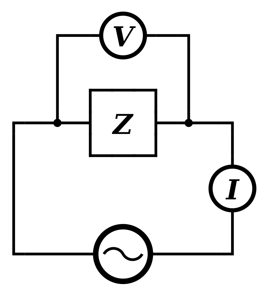
In one of my posts on oscillators, I explain the concept of impedance, which is the equivalent of resistance, but for AC circuits. Just like resistance, impedance also sort of measures the ‘opposition’ that a circuit presents to a current when a voltage is applied, but it’s a complex ratio, as opposed to R = V/I. It’s literally a complex ratio because the impedance has a magnitude and a direction, or a phase as it’s usually referred to. Hence, one will often write the impedance (denoted by Z) using Euler’s formula:

Z = |Z|e^iθ

The illustration below (credit goes to Wikipedia, once again) explains what’s going on. It’s a pretty generic view of the same AC circuit. The truth is: if we apply an alternating current, then the current and the voltage will both go up and down, but the current signal will usually lag the voltage signal, and the phase factor θ tells us by how much. Hence, using complex-number notation, we write:

V = I∗Z = I∗|Z|e^iθ

Now, while that resembles the V = R·I formula, you should note the bold-face type for V and I, and the ∗ symbol I am using here for multiplication. First the ∗ symbol: that’s to make it clear we’re not talking a vector cross product A×B here, but a product of two complex numbers. The bold-face for V and I implies they’re like vectors, or like complex numbers: so they have a phase too and, hence, we can write them as:

• V = |V|e^{i(ωt + θ_V)}
• I = |I|e^{i(ωt + θ_I)}

To be fully complete – you may skip all of this if you want, but it’s not that difficult, nor very long – it all works out as follows. We write:

V = I∗Z = |I|e^{i(ωt + θ_I)}∗|Z|e^iθ = |I||Z|e^{i(ωt + θ_I + θ)} = |V|e^{i(ωt + θ_V)}

Now, this equation must hold for all t, so we can equate the magnitudes and phases and, hence, we get: |V| = |I||Z| and so we get the formula we need, i.e. the phase difference between our function for the voltage and our function for the current.

θ_V = θ_I + θ

Of course, you’ll say: voltage and current are something real, isn’t it? So what’s this about complex numbers? You’re right. I’ve used the complex notation only to simplify the calculus, so it’s only the real part of those complex-valued functions that counts.

Oh… And also note that, as mentioned above, we do not have such lag or phase difference when only resistors are involved. So we don’t need the concept of impedance in the analysis above. With this addendum, I just wanted to be as complete as I can be. 🙂

Some content on this page was disabled on June 16, 2020 as a result of a DMCA takedown notice from The California Institute of Technology. You can learn more about the DMCA here:

https://wordpress.com/support/copyright-and-the-dmca/
Some content on this page was disabled on June 16, 2020 as a result of a DMCA takedown notice from The California Institute of Technology. You can learn more about the DMCA here:

https://wordpress.com/support/copyright-and-the-dmca/
Some content on this page was disabled on June 16, 2020 as a result of a DMCA takedown notice from The California Institute of Technology. You can learn more about the DMCA here:

https://wordpress.com/support/copyright-and-the-dmca/
Some content on this page was disabled on June 16, 2020 as a result of a DMCA takedown notice from The California Institute of Technology. You can learn more about the DMCA here:

https://wordpress.com/support/copyright-and-the-dmca/
Some content on this page was disabled on June 17, 2020 as a result of a DMCA takedown notice from Michael A. Gottlieb, Rudolf Pfeiffer, and The California Institute of Technology. You can learn more about the DMCA here:

https://wordpress.com/support/copyright-and-the-dmca/
Some content on this page was disabled on June 20, 2020 as a result of a DMCA takedown notice from Michael A. Gottlieb, Rudolf Pfeiffer, and The California Institute of Technology. You can learn more about the DMCA here:

https://wordpress.com/support/copyright-and-the-dmca/