My previous post discussed a more formal and “mainstream-compatible” paper on structured oscillatory fields, multipole geometry, and emergent interaction scales.
This new note goes in the opposite direction: radically simplified semi-classical reasoning using only rotating charge, Maxwellian current geometry, coupled oscillations, and elementary rotational dynamics.
Oddly enough, both approaches seem to converge toward similar intuitions about oscillatory structure and geometry in physics.
Perhaps progress sometimes comes not from moving in a straight line, but from oscillating between abstraction and simplicity.
Today I made a major step towards a very different Zitterbewegung model of a proton. With different, I mean different from the usual toroidal or helical model(s). I had a first version of this paper but the hyperlink gives you the updated paper. The update is small but very important: I checked all the formulas with ChatGPT and, hence, consider that as confirmation that I am on the right track. To my surprise, ChatGPT first fed me the wrong formula for an orbital frequency formula. Because I thought it could not be wrong on such simple matters, I asked it to check and double-check. It came with rather convincing geometrical explanations but I finally found an error in its reasoning, and the old formula from an online engineering textbook turned out to be correct.
In any case, I now have a sparring partner – ChatGPT o1 – to further develop the model that we finally settled on. That is a major breakthrough in this realistic interpretation of quantum theory and particle models that I have been trying to develop: the electron model is fine, and so now all that is left is this proton model. And then, of course, a model for a neutron or the deuteron nucleus. That will probably be a retirement project, or something for my next life. 🙂
Post scriptum: I followed up. “A theory’s value lies in its utility and ability to explain phenomena, regardless of whether it’s mainstream or not.” That’s ChatGPT’s conclusion after various explorations and chats with it over the past few weeks: https://lnkd.in/ekAAbvwc. I think I tried to push its limits when discussing problems in physics, leading it to make a rather remarkable distinction between “it’s” perspective and mine (see point 6 of Annex I of https://lnkd.in/eFVAyHn8), but – frankly – it may have no limits. As far as I can see, ChatGPT-o1 is truly amazing: sheer logic. 🙂 hashtag#AIhashtag#ChatGPThashtag#theoryofreality
I had been wanting to update my paper on matter-antimatter pair creation and annihilation for a long time, and I finally did it: here is the new version of it. It was one of my early papers on ResearchGate and, somewhat surprising, it got quite a few downloads (all is relative: I am happy with a few thousand). I actually did not know why, but now I understand: it does take down the last defenses of QCD- and QFT-theorists. As such, I now think this paper is at least as groundbreaking as my paper on de Broglie’s matter-wave (which gets the most reads), or my paper on the proton radius (which gets the most recommendations).
My paper on de Broglie’s matter-wave is important because it explains why and how de Broglie’s bright insight (matter having some frequency and wavelength) was correct, but got the wrong interpretation: the frequencies and wavelengths are orbital frequencies, and the wavelengths are are not to be interpreted as linear distances (not like wavelengths of light) but the quantum-mechanical equivalent of the circumferences of orbital radii. The paper also shows why spin (in this or the opposite direction) should be incorporated into any analysis straight from the start: you cannot just ignore spin and plug it in back later. The paper on the proton radius shows how that works to yield short and concise explanations of the measurable properties of elementary particles (the electron and the proton). The two combined provide the framework: an analysis of matter in terms of pointlike particles does not get us anywhere. We must think of matter as charge in motion, and we must analyze the two- or three-dimensional structure of these oscillations, and use it to also explain interactions between matter-particles (elementary or composite) and light-particles (photons and neutrinos, basically). I have explained these mass-without-mass models too many times now, so I will not dwell on it.
So, how that paper on matter-antimatter pair creation and annihilation fit in? The revision resulted in a rather long and verbose thing, so I will refer you to it and just summarize it very briefly. Let me start by copying the abstract: “The phenomenon of matter-antimatter pair creation and annihilation is usually taken as confirmation that, somehow, fields can condense into matter-particles or, conversely, that matter-particles can somehow turn into lightlike particles (photons and/or neutrinos, which are nothing but traveling fields: electromagnetic or, in the case of the neutrino, some strong field, perhaps). However, pair creation usually involves the presence of a nucleus or other charged particles (such as electrons in experiment #E144). We, therefore, wonder whether pair creation and annihilation cannot be analyzed as part of some nuclear process. To be precise, we argue that the usual nuclear reactions involving protons and neutrons can effectively account for the processes of pair creation and annihilation. We therefore argue that the need to invoke some quantum field theory (QFT) to explain these high-energy processes would need to be justified much better than it currently is.”
Needless to say, the last line above is a euphemism: we think our explanation is complete, and that QFT is plain useless. We wrote the following rather scathing appreciation of it in a footnote of the paper: “We think of Aitchison & Hey’s presentation of [matter-antimatter pair creation and annihilation] in their Gauge Theories in Particle Physics (2012) – or presentations (plural), we should say. It is considered to be an advanced but standard textbook on phenomena like this. However, one quickly finds oneself going through the index and scraping together various mathematical treatments – wondering what they explain, and also wondering how all of the unanswered questions or hypotheses (such as, for example, the particularities of flavor mixing, helicity, the Majorana hypothesis, etcetera) contribute to understanding the nature of the matter at hand. I consider it a typical example of how – paraphrasing Sabine Hossenfelder’s judgment on the state of advanced physics research – physicist do indeed tend to get lost in math.”
That says it all. Our thesis is that charge cannot just appear or disappear: it is not being created out of nothing (or out of fields, we should say). The observations (think of pion production and decay from cosmic rays here) and the results of the experiments (the mentioned #E144 experiment or other high-energy experiments) cannot be disputed, but the mainstream interpretation of what actually happens or might be happening in those chain reactions suffers from what, in daily life, we would refer to as ‘very sloppy accounting’. Let me quote or paraphrase a few more lines from my paper to highlight the problem, and to also introduce my interpretation of things which, as usual, are based on a more structural analysis of what matter actually is:
“Pair creation is most often observed in the presence of a nucleus. The role of the nucleus is usually reduced to that of a heavy mass only: it only appears in the explanation to absorb or provide some kinetic energy in the overall reaction. We instinctively feel the role of the nucleus must be far more important than what is usually suggested. To be specific, we suggest pair creation should (also) be analyzed as being part of a larger nuclear process involving neutron-proton interactions. […]”
“Charge does not get ‘lost’ or is ‘created’, but [can] switch its ‘spacetime’ or ‘force’ signature [when interacting with high-energy (anti)photons or (anti)neutrinos].”
“[The #E144 experiment or other high-energy experiments involving electrons] accounts for the result of the experiment in terms of mainstream QED analysis, and effectively thinks of the pair production being the result of the theoretical ‘Breit-Wheeler’ pair production process from photons only. However, this description of the experiment fails to properly account for the incoming beam of electrons. That, then, is the main weakness of the ‘explanation’: it is a bit like making abstraction of the presence of the nucleus in the pair creation processes that take place near them (which, as mentioned above, account for the bulk of those).”
We will say nothing more about it here because we want to keep our blog post(s) short: read the paper! 🙂 To wrap this up for you, the reader(s) of this post, we will only quote or paraphrase some more ontological or philosophical remarks in it:
“The three-layered structure of the electron (the classical, Compton and Bohr radii of the electron) suggest that charge may have some fractal structure and – moreover – that such fractal structure may be infinite. Why do we think so? If the fractal structure would not be infinite, we would have to acknowledge – logically – that some kind of hard core charge is at the center of the oscillations that make up these particles, and it would be very hard to explain how this can actually disappear.” [Note: This is a rather novel new subtlety in our realist interpretation of quantum physics, so you may want to think about it. Indeed, we were initially not very favorable to the idea of a fractal charge structure because such fractal structure is, perhaps, not entirely consistent with the idea of a Zitterbewegung charge with zero rest mass), we think much more favorably of the hypothesis now.]
“The concept of charge is and remains mysterious. However, in philosophical or ontological terms, I do not think of it as a mystery: at some point, we must, perhaps, accept that the essence of the world is charge, and that:
There is also an antiworld, and that;
It consists of an anticharge that we can fully define in terms of the signature of the force(s) that keep it together, and that;
The two worlds can, quite simply, not co-exist or – at least – not interact with each other without annihilating each other.
Such simple view of things must, of course, feed into cosmological theories: how, then, came these two worlds into being? We offered some suggestions on that in a rather simple paper on cosmology (our one and only paper on the topic), but it is not a terrain that we have explored (yet).”
So, I will end this post in pretty much the same way as the old Looney Tunes or Merrie Melodies cartoons used to end, and that’s by saying: “That’s all Folks.” 🙂
Enjoy life and do not worry too much. It is all under control and, if it is not, then that is OK too. 🙂
In this blog, we talked a lot about the Zitterbewegung model of an electron, which is a model which allows us to think of the elementary wavefunction as representing a radius or position vector. We write:
ψ = r = a·e±iθ = a·[cos(±θ) + i · sin(±θ)]
It is just an application of Parson’s ring current or magneton model of an electron. Note we use boldface to denote vectors, and that we think of the sine and cosine here as vectors too! You should note that the sine and cosine are the same function: they differ only because of a 90-degree phase shift: cosθ = sin(θ + π/2). Alternatively, we can use the imaginary unit (i) as a rotation operator and use the vector notation to write: sinθ = i·cosθ.
In one of our introductory papers (on the language of math), we show how and why this all works like a charm: when we take the derivative with respect to time, we get the (orbital or tangential) velocity (dr/dt = v), and the second-order derivative gives us the (centripetal) acceleration vector (d2r/dt2 = a). The plus/minus sign of the argument of the wavefunction gives us the direction of spin, and we may, perhaps, add a plus/minus sign to the wavefunction as a whole to model matter and antimatter, respectively (the latter assertion is very speculative though, so we will not elaborate that here).
One orbital cycle packs Planck’s quantum of (physical) action, which we can write either as the product of the energy (E) and the cycle time (T), or the momentum (p) of the charge times the distance travelled, which is the circumference of the loop λ in the inertial frame of reference (we can always add a classical linear velocity component when considering an electron in motion, and we may want to write Planck’s quantum of action as an angular momentum vector (h or ħ) to explain what the Uncertainty Principle is all about (statistical uncertainty, nothing ontological), but let us keep things simple as for now):
h = E·T = p·λ
It is important to distinguish between the electron and the charge, which we think of being pointlike: the electron is charge in motion. Charge is just charge: it explains everything and its nature is, therefore, quite mysterious: is it really a pointlike thing, or is there some fractal structure? Of these things, we know very little, but the small anomaly in the magnetic moment of an electron suggests its structure might be fractal. Think of the fine-structure constant here, as the factor which distinguishes the classical, Compton and Bohr radii of the electron: we associate the classical electron radius with the radius of the poinlike charge, but perhaps we can drill down further.
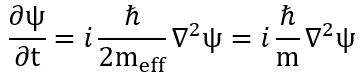
We also showed how the physical dimensions work out in Schroedinger’s wave equation. Let us jot it down to appreciate what it might model, and appreciate why complex numbers come in handy:
Schroedinger’s equation in free space
This is, of course, Schroedinger’s equation in free space, which means there are no other charges around and we, therefore, have no potential energy terms here. The rather enigmatic concept of the effective mass (which is half the total mass of the electron) is just the relativistic mass of the pointlike charge as it whizzes around at lightspeed, so that is the motion which Schroedinger referred to as its Zitterbewegung (Dirac confused it with some motion of the electron itself, further compounding what we think of as de Broglie’s mistaken interpretation of the matter-wave as a linear oscillation: think of it as an orbital oscillation). The 1/2 factor is there in Schroedinger’s wave equation for electron orbitals, but he replaced the effective mass rather subtly (or not-so-subtly, I should say) by the total mass of the electron because the wave equation models the orbitals of an electron pair (two electrons with opposite spin). So we might say he was lucky: the two mistakes together (not accounting for spin, and adding the effective mass of two electrons to get a mass factor) make things come out alright. 🙂
However, we will not say more about Schroedinger’s equation for the time being (we will come back to it): just note the imaginary unit, which does operate like a rotation operator here. Schroedinger’s wave equation, therefore, must model (planar) orbitals. Of course, the plane of the orbital itself may be rotating itself, and most probably is because that is what gives us those wonderful shapes of electron orbitals (subshells). Also note the physical dimension of ħ/m: it is a factor which is expressed in m2/s, but when you combine that with the 1/m2 dimension of the ∇2 operator, then you get the 1/s dimension on both sides of Schroedinger’s equation. [The ∇2 operator is just the generalization of the d2r/dx2 but in three dimensions, so x becomes a vector: x, and we apply the operator to the three spatial coordinates and get another vector, which is why we call ∇2 a vector operator. Let us move on, because we cannot explain each and every detail here, of course!]
We need to talk forces and fields now. This ring current model assumes an electromagnetic field which keeps the pointlike charge in its orbit. This centripetal force must be equal to the Lorentz force (F), which we can write in terms of the electric and magnetic field vectors E and B (fields are just forces per unit charge, so the two concepts are very intimately related):
We use a different imaginary unit here (j instead of i) because the plane in which the magnetic field vector B is going round and round is orthogonal to the plane in which E is going round and round, so let us call these planes the xy– and xz-planes respectively. Of course, you will ask: why is the B-plane not the yz-plane? We might be mistaken, but the magnetic field vector lags the electric field vector, so it is either of the two, and so now you can check for yourself of what we wrote above is actually correct. Also note that we write 1 as a vector (1) or a complex number: 1 = 1 + i·0. [It is also possible to write this: 1 = 1 + i·0 or 1 = 1 + i·0. As long as we think of these things as vectors – something with a magnitude and a direction – it is OK.]
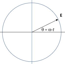
You may be lost in math already, so we should visualize this. Unfortunately, that is not easy. You may to google for animations of circularly polarized electromagnetic waves, but these usually show the electric field vector only, and animations which show bothE and B are usually linearly polarized waves. Let me reproduce the simplest of images: imagine the electric field vector E going round and round. Now imagine the field vector B being orthogonal to it, but also going round and round (because its phase follows the phase of E). So, yes, it must be going around in the xz– or yz-plane (as mentioned above, we let you figure out how the various right-hand rules work together here).
Rotational plane of the electric field vector
You should now appreciate that the E and B vectors – taken together – will also form a plane. This plane is not static: it is not the xy-, yz– or xz-plane, nor is it some static combination of two of these. No! We cannot describe it with reference to our classical Cartesian axes because it changes all the time as a result of the rotation of both the E and B vectors. So how we can describe that plane mathematically?
The Irish mathematician William Rowan Hamilton – who is also known for many other mathematical concepts – found a great way to do just that, and we will use his notation. We could say the plane formed by the E and B vectors is the E–B plane but, in line with Hamilton’s quaternion algebra, we will refer to it as the k-plane. How is it related to what we referred to as the i– and j-planes, or the xy– and xz-plane as we used to say? At this point, we should introduce Hamilton’s notation: he did write i and j in boldface (we do not like that, but you may want to think of it as just a minor change in notation because we are using these imaginary units in a new mathematical space: the quaternion number space), and he referred to them as basic quaternions in what you should think of as an extension of the complex number system. More specifically, he wrote this on a now rather famous bridge in Dublin:
i2 = -1
j2 = -1
k2 = -1
i·j = k
j·i= –k
The first three rules are the ones you know from complex number math: two successive rotations by 90 degrees will bring you from 1 to -1. The order of multiplication in the other two rules ( i·j = k and j·i = –k ) gives us not only the k-plane but also the spin direction. All other rules in regard to quaternions (we can write, for example, this: i ·j·k = -1), and the other products you will find in the Wikipedia article on quaternions) can be derived from these, but we will not go into them here.
Now, you will say, we do not really need that k, do we? Just distinguishing between i and j should do, right? The answer to that question is: yes, when you are dealing with electromagnetic oscillations only! But it is no when you are trying to model nuclear oscillations! That is, in fact, exactly why we need this quaternion math in quantum physics!
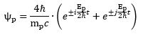
Let us think about this nuclear oscillation. Particle physics experiments – especially high-energy physics experiments – effectively provide evidence for the presence of a nuclear force. To explain the proton radius, one can effectively think of a nuclear oscillation as an orbital oscillation in three rather than just two dimensions. The oscillation is, therefore, driven by two (perpendicular) forces rather than just one, with the frequency of each of the oscillators being equal to ω = E/2ħ = mc2/2ħ.
Each of the two perpendicular oscillations would, therefore, pack one half-unit of ħ only. The ω = E/2ħ formula also incorporates the energy equipartition theorem, according to which each of the two oscillations should pack half of the total energy of the nuclear particle (so that is the proton, in this case). This spherical view of a proton fits nicely with packing models for nucleons and yields the experimentally measured radius of a proton:
Proton radius formula
Of course, you can immediately see that the 4 factor is the same factor 4 as the one appearing in the formula for the surface area of a sphere (A = 4πr2), as opposed to that for the surface of a disc (A = πr2). And now you should be able to appreciate that we should probably represent a proton by a combination of two wavefunctions. Something like this:
Proton wavefunction
What about a wave equation for nuclear oscillations? Do we need one? We sure do. Perhaps we do not need one to model a neutron as some nuclear dance of a negative and a positive charge. Indeed, think of a combination of a proton and what we will refer to as a deep electron here, just to distinguish it from an electron in Schroedinger’s atomic electron orbitals. But we might need it when we are modeling something more complicated, such as the different energy states of, say, a deuteron nucleus, which combines a proton and a neutron and, therefore, two positive charges and one deep electron.
According to some, the deep electron may also appear in other energy states and may, therefore, give rise to a different kind of hydrogen (they are referred to as hydrinos). What do I think of those? I think these things do not exist and, if they do, they cannot be stable. I also think these researchers need to come up with a wave equation for them in order to be credible and, in light of what we wrote about the complications in regard to the various rotational planes, that wave equation will probably have all of Hamilton’s basic quaternions in it. [But so, as mentioned above, I am waiting for them to come up with something that makes sense and matches what we can actually observe in Nature: those hydrinos should have a specific spectrum, and we do not such see such spectrum from, say, the Sun, where there is so much going on so, if hydrinos exist, the Sun should produce them, right? So, yes, I am rather skeptical here: I do think we know everything now and physics, as a science, is sort of complete and, therefore, dead as a science: all that is left now is engineering!]
But, yes, quaternion algebra is a very necessary part of our toolkit. It completes our description of everything! 🙂
Pre-scriptum (6 February 2021): We solved this one. The proton is, effectively, a 3D zbw oscillation (as opposed to the 2D oscillation of the pointlike charge in an electron. See our latest paper on the nuclear force.
Our alternative realist interpretation of quantum physics is pretty complete but one thing that has been puzzling us is the mass density of a proton: why is it so massive as compared to an electron? We simplified things by adding a factor in the Planck-Einstein relation. To be precise, we wrote it as E = 4·h·f. This allowed us to derive the proton radius from the ring current model:
This felt a bit artificial. Writing the Planck-Einstein relation using an integer multiple of h or ħ (E = n·h·f = n·ħ·ω) is not uncommon. You should have encountered this relation when studying the black-body problem, for example, and it is also commonly used in the context of Bohr orbitals of electrons. But why is n equal to 4 here? Why not 2, or 3, or 5 or some other integer? We do not know: all we know is that the proton is very different. A proton is, effectively, not the antimatter counterpart of an electron—a positron. While the proton is much smaller – 459 times smaller, to be precise – its mass is 1,836 times that of the electron. Note that we have the same 1/4 factor here because the mass and Compton radius are inversely proportional:
This doesn’t look all that bad but it feels artificial. In addition, our reasoning involved a unexplained difference – a mysterious but exact SQRT(2) factor, to be precise – between the theoretical and experimentally measured magnetic moment of a proton. In short, we assumed some form factor must explain both the extraordinary mass density as well as this SQRT(2) factor but we were not quite able to pin it down, exactly. A remark on a video on our YouTube channel inspired us to think some more – thank you for that, Andy! – and we think we may have the answer now.
We now think the mass – or energy – of a proton combines two oscillations: one is the Zitterbewegung oscillation of the pointlike charge (which is a circular oscillation in a plane) while the other is the oscillation of the plane itself. The illustration below is a bit horrendous (I am not so good at drawings) but might help you to get the point. The plane of the Zitterbewegung (the plane of the proton ring current, in other words) may oscillate itself between +90 and −90 degrees. If so, the effective magnetic moment will differ from the theoretical magnetic moment we calculated, and it will differ by that SQRT(2) factor.
Hence, we should rewrite our paper, but the logic remains the same: we just have a much better explanation now of why we should apply the energy equipartition theorem.
Mystery solved! 🙂
Post scriptum (9 August 2020): The solution is not as simple as you may imagine. When combining the idea of some other motion to the ring current, we must remember that the speed of light – the presumed tangential speed of our pointlike charge – cannot change. Hence, the radius must become smaller. We also need to think about distinguishing two different frequencies, and things quickly become quite complicated.
I’ve been working across Asia – mainly South Asia – for over 25 years now. You will google the exact meaning but my definition of a wallah is a someone who deals in something: it may be a street vendor, or a handyman, or anyone who brings something new. I remember I was one of the first to bring modern mountain bikes to India, and they called me a gear wallah—because they were absolute fascinated with the number of gears I had. [Mountain bikes are now back to a 2 by 10 or even a 1 by 11 set-up, but I still like those three plateaux in front on my older bikes—and, yes, my collection is becoming way too large but I just can’t do away with it.]
It just makes me wonder: why is the outcome of this 100-year old battle between mainstream hocus-pocus and real physics so undecided?
I’ve come to think of mainstream physicists as peddlers in mysteries—whence the title of my post. It’s a tough conclusion. Physics is supposed to be the King of Science, right? Hence, we shouldn’t doubt it. At the same time, it is kinda comforting to know the battle between truth and lies rages everywhere—including inside of the King of Science.
I thought I’d stop blogging, but I can’t help it: I think you’d find this topic interesting – and my comments are actually too short for a paper or article, so I thought it would be good to throw it out here.
If you follow the weird world of quantum mechanics with some interest, you will have heard the latest news: the ‘puzzle’ of the charge radius of the proton has been solved. To be precise, a more precise electron-proton scattering experiment by the PRad (proton radius) team using the Continuous Electron Beam Accelerator Facility (CEBAF) at Jefferson Lab has now measured the root mean square (rms) charge radius of the proton as[1]:
rp = 0.831 ± 0.007stat ± 0.012syst fm
If a proton would, somehow, have a pointlike elementary (electric) charge in it, and if it it is in some kind of circular motion (as we presume in Zitterbewegung models of elementary particles), then we can establish a simple relation between the magnetic moment (μ) and the radius (a) of the circular current.
Indeed, the magnetic moment is the current (I) times the surface area of the loop (πa2), and the current is just the product of the elementary charge (qe) and the frequency (f), which we can calculate as f = c/2πa, i.e. the velocity of the charge[2] divided by the circumference of the loop. We write:Using the Compton radius of an electron (ae = ħ/mec), this yields the correct magnetic moment for the electron[3]:What radius do we get when applying the a = μ/0.24…´10–10 relation to the (experimentally measured) magnetic moment of a proton? I invite the reader to verify the next calculation using CODATA values:When I first calculated this, I thought: that’s not good enough. I only have the order of magnitude right. However, when multiplying this with √2, we get a value which fits into the 0.831 ± 0.007 interval. To be precise, we get this:
Of course, you will wonder: how can we justify the √2 factor? I am not sure. It is a charge radius. Hence, the electrons will bounce off because of the electromagnetic fields. The magnetic field of the current ring will be some envelope to the current ring itself. We would, therefore, expect the measured charge radius to be larger than the radius of the current ring (a). There are also the intricacies related to the definition of a root mean square (rms) radius.
I feel this cannot be a coincidence: the difference between our ‘theoretical’ value (0.83065 fm) and the last precision measurement (0.831 fm) is only 0.00035 fm, which is only 5% of the statistical standard deviation (0.007 fm). Proton radius solved?
Maybe. Maybe not. The concluding comments of Physics Today were this: “The PRad radius result, about 0.83 fm, agrees with the smaller value from muonic and now electronic hydrogen spectroscopy measurements. With that, it seems the puzzle is resolved, and the discrepancy was likely due to measurement errors. Unfortunately, the conclusion requires no new physics.” (my italics)
I wonder what kind of new physics they are talking about.
Jean Louis Van Belle, 24 January 2020
PS: I did make a paper out of this (see my academia.edu or viXra.org publications), and I shared it with the PRad team at JLAB. Prof. Dr. Ashot Gasparian was kind enough to acknowledge my email and thought “the approach and numbers are interesting.” Let us see what comes out of it. I need to get back to my day job. 🙂
[2]Zitterbewegung models assume an electron consists of a pointlike charge whizzing around some center. The rest mass of the pointlike charge is zero, which is why its velocity is equal to the speed of light. However, because of its motion, it acquires an effective mass – pretty much like a photon, which has mass because of its motion. One can show the effective mass of the pointlike charge – which is a relativistic mass concept – is half the rest mass of the electron: mγ = me/2.
[3] The calculations do away with the niceties of the + or – sign conventions as they focus on the values only. We also invite the reader to add the SI units so as to make sure all equations are consistent from a dimensional point of view. For the values themselves, see the CODATA values on the NIST website (https://physics.nist.gov/cuu/Constants/index.html).