Re-visiting the matter wave (II)

Pre-scriptum (dated 26 June 2020): This post did not suffer too much from the DMCA take-down of some material: only one or two illustrations from Feynman’s Lectures were removed. It is, therefore, still quite readable—even if my views on these  matters have evolved quite a bit as part of my realist interpretation of QM. I have actually re-written Feynman’s first lectures of quantum mechanics to replace de Broglie’s concept of the matter-wave with what I think is a much better description of ‘wavicles’: one that fully captures their duality. That paper has got the same title (Quantum Behavior) as Feynman’s first lecture but you will see it is a totally different animal. 🙂

So you should probably not read the post below but my lecture(s) instead. 🙂 This is the link to the first one, and here you can look at the second one. Both taken together are an alternative treatment of the subject-matter which Feynman’s discusses in Lecture 1 to 9 of his Lectures (I use a big L for his lectures to show the required reverence for all of the Mystery Wallahs—Feynman included). Let me know what you think of them (I mean the lectures here, not the mystery wallahs).

Original post:

My previous post was, once again, littered with formulas – even if I had not intended it to be that way: I want to convey some kind of understanding of what an electron – or any particle at the atomic scale – actually is – with the minimum number of formulas necessary.

We know particles display wave behavior: when an electron beam encounters an obstacle or a slit that is somewhat comparable in size to its wavelength, we’ll observe diffraction, or interference. [I have to insert a quick note on terminology here: the terms diffraction and interference are often used interchangeably, but there is a tendency to use interference when we have more than one wave source and diffraction when there is only one wave source. However, I’ll immediately add that distinction is somewhat artificial. Do we have one or two wave sources in a double-slit experiment? There is one beam but the two slits break it up in two and, hence, we would call it interference. If it’s only one slit, there is also an interference pattern, but the phenomenon will be referred to as diffraction.]

We also know that the wavelength we are talking about it here is not the wavelength of some electromagnetic wave, like light. It’s the wavelength of a de Broglie wave, i.e. a matter wave: such wave is represented by an (oscillating) complex number – so we need to keep track of a real and an imaginary part – representing a so-called probability amplitude Ψ(x, t) whose modulus squared (│Ψ(x, t)│2) is the probability of actually detecting the electron at point x at time t. [The purists will say that complex numbers can’t oscillate – but I am sure you get the idea.]

You should read the phrase above twice: we cannot know where the electron actually is. We can only calculate probabilities (and, of course, compare them with the probabilities we get from experiments). Hence, when the wave function tells us the probability is greatest at point x at time t, then we may be lucky when we actually probe point x at time t and find it there, but it may also not be there. In fact, the probability of finding it exactly at some point x at some definite time t is zero. That’s just a characteristic of such probability density functions: we need to probe some region Δx in some time interval Δt.

If you think that is not very satisfactory, there’s actually a very common-sense explanation that has nothing to do with quantum mechanics: our scientific instruments do not allow us to go beyond a certain scale anyway. Indeed, the resolution of the best electron microscopes, for example, is some 50 picometer (1 pm = 1×10–12 m): that’s small (and resolutions get higher by the year), but so it implies that we are not looking at points – as defined in math that is: so that’s something with zero dimension – but at pixels of size Δx = 50×10–12 m.

The same goes for time. Time is measured by atomic clocks nowadays but even these clocks do ‘tick’, and these ‘ticks’ are discrete. Atomic clocks take advantage of the property of atoms to resonate at extremely consistent frequencies. I’ll say something more about resonance soon – because it’s very relevant for what I am writing about in this post – but, for the moment, just note that, for example, Caesium-133 (which was used to build the first atomic clock) oscillates at 9,192,631,770 cycles per second. In fact, the International Bureau of Standards and Weights re-defined the (time) second in 1967 to correspond to “the duration of 9,192,631,770 periods of the radiation corresponding to the transition between the two hyperfine levels of the ground state of the Caesium-133 atom at rest at a temperature of 0 K.”

Don’t worry about it: the point to note is that when it comes to measuring time, we also have an uncertainty. Now, when using this Caesium-133 atomic clock, this uncertainty would be in the range of ±9.2×10⁻⁹ seconds (so that’s nanoseconds: 1 ns = 1×10⁻⁹ s), because that’s the rate at which this clock ‘ticks’. However, there are other (much more plausible) ways of measuring time: some of the unstable baryons have lifetimes in the range of a few picoseconds only (1 ps = 1×10–12 s) and the really unstable ones – known as baryon resonances – have lifetimes in the 1×10–22 to 1×10–24 s range. This we can only measure because they leave some trace after these particle collisions in particle accelerators and, because we have some idea about their speed, we can calculate their lifetime from the (limited) distance they travel before disintegrating. The thing to remember is that for time also, we have to make do with time pixels  instead of time points, so there is a Δt as well. [In case you wonder what baryons are: they are particles consisting of three quarks, and the proton and the neutron are the most prominent (and most stable) representatives of this family of particles.]  

So what’s the size of an electron? Well… It depends. We need to distinguish two very different things: (1) the size of the area where we are likely to find the electron, and (2) the size of the electron itself. Let’s start with the latter, because that’s the easiest question to answer: there is a so-called classical electron radius re, which is also known as the Thompson scattering length, which has been calculated as:

r_\mathrm{e} = \frac{1}{4\pi\varepsilon_0}\frac{e^2}{m_{\mathrm{e}} c^2} = 2.817 940 3267(27) \times 10^{-15} \mathrm{m}As for the constants in this formula, you know these by now: the speed of light c, the electron charge e, its mass me, and the permittivity of free space εe. For whatever it’s worth (because you should note that, in quantum mechanics, electrons do not have a size: they are treated as point-like particles, so they have a point charge and zero dimension), that’s small. It’s in the femtometer range (1 fm = 1×10–15 m). You may or may not remember that the size of a proton is in the femtometer range as well – 1.7 fm to be precise – and we had a femtometer size estimate for quarks as well: 0.7 m. So we have the rather remarkable result that the much heavier proton (its rest mass is 938 MeV/csas opposed to only 0.511 MeV MeV/c2, so the proton is 1835 times heavier) is 1.65 times smaller than the electron. That’s something to be explored later: for the moment, we’ll just assume the electron wiggles around a bit more – exactly because it’s lighterHere you just have to note that this ‘classical’ electron radius does measure something: it’s something ‘hard’ and ‘real’ because it scatters, absorbs or deflects photons (and/or other particles). In one of my previous posts, I explained how particle accelerators probe things at the femtometer scale, so I’ll refer you to that post (End of the Road to Reality?) and move on to the next question.

The question concerning the area where we are likely to detect the electron is more interesting in light of the topic of this post (the nature of these matter waves). It is given by that wave function and, from my previous post, you’ll remember that we’re talking the nanometer scale here (1 nm = 1×10⁻⁹ m), so that’s a million times larger than the femtometer scale. Indeed, we’ve calculated a de Broglie wavelength of 0.33 nanometer for relatively slow-moving electrons (electrons in orbit), and the slits used in single- or double-slit experiments with electrons are also nanotechnology. In fact, now that we are here, it’s probably good to look at those experiments in detail.

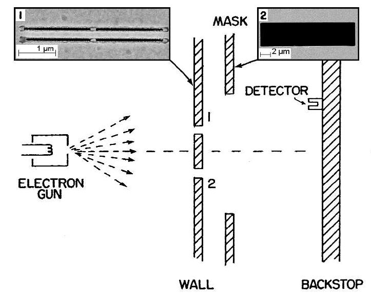
The illustration below relates the actual experimental set-up of a double-slit experiment performed in 2012 to Feynman’s 1965 thought experiment. Indeed, in 1965, the nanotechnology you need for this kind of experiment was not yet available, although the phenomenon of electron diffraction had been confirmed experimentally already in 1925 in the famous Davisson-Germer experiment. [It’s famous not only because electron diffraction was a weird thing to contemplate at the time but also because it confirmed the de Broglie hypothesis only two years after Louis de Broglie had advanced it!]. But so here is the experiment which Feynman thought would never be possible because of technology constraints:

Electron double-slit set-upThe insert in the upper-left corner shows the two slits: they are each 50 nanometer wide (50×10–9 m) and 4 micrometer tall (4×10⁻⁶ m). [The thing in the middle of the slits is just a little support. Please do take a few seconds to contemplate the technology behind this feat: 50 nm is 50 millionths of a millimeter. Try to imagine dividing one millimeter in ten, and then one of these tenths in ten again, and again, and once again, again, and again. You just can’t imagine that, because our mind is used to addition/subtraction and – to some extent – with multiplication/division: our mind can’t deal with with exponentiation really – because it’s not a everyday phenomenon.] The second inset (in the upper-right corner) shows the mask that can be moved to close one or both slits partially or completely.

Now, 50 nanometer is 150 times larger than the 0.33 nanometer range we got for ‘our’ electron, but it’s small enough to show diffraction and/or interference. [In fact, in this experiment (done by Bach, Pope, Liou and Batelaan from the University of Nebraska-Lincoln less than two years ago indeed), the beam consisted of electrons with an (average) energy of 600 eV and a de Broglie wavelength of 50 picometer. So that’s like the electrons used in electron microscopes. 50 pm is 6.6 times smaller than the 0.33 nm wavelength we calculated for our low-energy (70 eV) electron – but then the energy and the fact these electrons are guided in electromagnetic fields explain the difference. Let’s go to the results.

The illustration below shows the predicted pattern next to the observed pattern for the two scenarios:

  1. We first close slit 2, let a lot of electrons go through it, and so we get a pattern described by the probability density function P1 = │Φ12. Here we see no interference but a typical diffraction pattern: the intensity follows a more or less normal (i.e. Gaussian) distribution. We then close slit 1 (and open slit 2 again), again let a lot of electrons through, and get a pattern described by the probability density function P2 = │Φ22. So that’s how we get P1 and P2.
  2. We then open both slits, let a whole electrons through, and get according to the pattern described by probability density function P12 = │Φ122, which we get not from adding the probabilities P1 and P2 (hence, P12 ≠  P1 + P2) – as one would expect if electrons would behave like particles – but from adding the probability amplitudes. We have interference, rather than diffraction.

Predicted interference effectBut so what exactly is interfering? Well… The electrons. But that can’t be, can it?

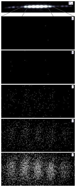
The electrons are obviously particles, as evidenced from the impact they make – one by one – as they hit the screen as shown below. [If you want to know what screen, let me quote the researchers: “The resulting patterns were magnified by an electrostatic quadrupole lens and imaged on a two-dimensional microchannel plate and phosphorus screen, then recorded with a charge-coupled device camera. […] To study the build-up of the diffraction pattern, each electron was localized using a “blob” detection scheme: each detection was replaced by a blob, whose size represents the error in the localization of the detection scheme. The blobs were compiled together to form the electron diffraction patterns.” So there you go.]

Electron blobs

Look carefully at how this interference pattern becomes ‘reality’ as the electrons hit the screen one by one. And then say it: WAW ! 

Indeed, as predicted by Feynman (and any other physics professor at the time), even if the electrons go through the slits one by one, they will interfere – with themselves so to speak. [In case you wonder if these electrons really went through one by one, let me quote the researchers once again: “The electron source’s intensity was reduced so that the electron detection rate in the pattern was about 1 Hz. At this rate and kinetic energy, the average distance between consecutive electrons was 2.3 × 10⁶ meters. This ensures that only one electron is present in the 1 meter long system at any one time, thus eliminating electron-electron interactions.” You don’t need to be a scientist or engineer to understand that, isn’t it?]

While this is very spooky, I have not seen any better way to describe the reality of the de Broglie wave: the particle is not some point-like thing but a matter wave, as evidenced from the fact that it does interfere with itself when forced to move through two slits – or through one slit, as evidenced by the diffraction patterns built up in this experiment when closing one of the two slits: the electrons went through one by one as well!

But so how does it relate to the characteristics of that wave packet which I described in my previous post? Let me sum up the salient conclusions from that discussion:

  1. The wavelength λ of a wave packet is calculated directly from the momentum by using de Broglie‘s second relation: λ = h/p. In this case, the wavelength of the electrons averaged 50 picometer. That’s relatively small as compared to the width of the slit (50 nm) – a thousand times smaller actually! – but, as evidenced by the experiment, it’s small enough to show the ‘reality’ of the de Broglie wave.
  2. From a math point (but, of course, Nature does not care about our math), we can decompose the wave packet in a finite or infinite number of component waves. Such decomposition is referred to, in the first case (finite number of composite waves or discrete calculus) as a Fourier analysis, or, in the second case, as a Fourier transform. A Fourier transform maps our (continuous) wave function, Ψ(x), to a (continuous) wave function in the momentum space, which we noted as φ(p). [In fact, we noted it as Φ(p) but I don’t want to create confusion with the Φ symbol used in the experiment, which is actually the wave function in space, so Ψ(x) is Φ(x) in the experiment – if you know what I mean.] The point to note is that uncertainty about momentum is related to uncertainty about position. In this case, we’ll have pretty standard electrons (so not much variation in momentum), and so the location of the wave packet in space should be fairly precise as well.
  3. The group velocity of the wave packet (vg) – i.e. the envelope in which our Ψ wave oscillates – equals the speed of our electron (v), but the phase velocity (i.e. the speed of our Ψ wave itself) is superluminal: we showed it’s equal to (vp) = E/p =   c2/v = c/β, with β = v/c, so that’s the ratio of the speed of our electron and the speed of light. Hence, the phase velocity will always be superluminal but will approach c as the speed of our particle approaches c. For slow-moving particles, we get astonishing values for the phase velocity, like more than a hundred times the speed of light for the electron we looked at in our previous post. That’s weird but it does not contradict relativity: if it helps, one can think of the wave packet as a modulation of an incredibly fast-moving ‘carrier wave’. 

Is any of this relevant? Does it help you to imagine what the electron actually is? Or what that matter wave actually is? Probably not. You will still wonder: How does it look like? What is it in reality?

That’s hard to say. If the experiment above does not convey any ‘reality’ according to you, then perhaps the illustration below will help. It’s one I have used in another post too (An Easy Piece: Introducing Quantum Mechanics and the Wave Function). I took it from Wikipedia, and it represents “the (likely) space in which a single electron on the 5d atomic orbital of an atom would be found.” The solid body shows the places where the electron’s probability density (so that’s the squared modulus of the probability amplitude) is above a certain value – so it’s basically the area where the likelihood of finding the electron is higher than elsewhere. The hue on the colored surface shows the complex phase of the wave function.

Hydrogen_eigenstate_n5_l2_m1

So… Does this help? 

You will wonder why the shape is so complicated (but it’s beautiful, isn’t it?) but that has to do with quantum-mechanical calculations involving quantum-mechanical quantities such as spin and other machinery which I don’t master (yet). I think there’s always a bit of a gap between ‘first principles’ in physics and the ‘model’ of a real-life situation (like a real-life electron in this case), but it’s surely the case in quantum mechanics! That being said, when looking at the illustration above, you should be aware of the fact that you are actually looking at a 3D representation of the wave function of an electron in orbit. 

Indeed, wave functions of electrons in orbit are somewhat less random than – let’s say – the wave function of one of those baryon resonances I mentioned above. As mentioned in my Not So Easy Piece, in which I introduced the Schrödinger equation (i.e. one of my previous posts), they are solutions of a second-order partial differential equation – known as the Schrödinger wave equation indeed – which basically incorporates one key condition: these solutions – which are (atomic or molecular) ‘orbitals’ indeed – have to correspond to so-called stationary states or standing waves. Now what’s the ‘reality’ of that? 

The illustration below comes from Wikipedia once again (Wikipedia is an incredible resource for autodidacts like me indeed) and so you can check the article (on stationary states) for more details if needed. Let me just summarize the basics:

  1. A stationary state is called stationary because the system remains in the same ‘state’ independent of time. That does not mean the wave function is stationary. On the contrary, the wave function changes as function of both time and space – Ψ = Ψ(x, t) remember? – but it represents a so-called standing wave.
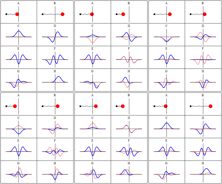
  2. Each of these possible states corresponds to an energy state, which is given through the de Broglie relation: E = hf. So the energy of the state is proportional to the oscillation frequency of the (standing) wave, and Planck’s constant is the factor of proportionality. From a formal point of view, that’s actually the one and only condition we impose on the ‘system’, and so it immediately yields the so-called time-independent Schrödinger equation, which I briefly explained in the above-mentioned Not So Easy Piece (but I will not write it down here because it would only confuse you even more). Just look at these so-called harmonic oscillators below:

QuantumHarmonicOscillatorAnimation

A and B represent a harmonic oscillator in classical mechanics: a ball with some mass m (mass is a measure for inertia, remember?) on a spring oscillating back and forth. In case you’d wonder what the difference is between the two: both the amplitude as well as the frequency of the movement are different. 🙂 A spring and a ball?

It represents a simple system. A harmonic oscillation is basically a resonance phenomenon: springs, electric circuits,… anything that swings, moves or oscillates (including large-scale things such as bridges and what have you – in his 1965 Lectures (Vol. I-23), Feynman even discusses resonance phenomena in the atmosphere in his Lectures) has some natural frequency ω0, also referred to as the resonance frequency, at which it oscillates naturally indeed: that means it requires (relatively) little energy to keep it going. How much energy it takes exactly to keep them going depends on the frictional forces involved: because the springs in A and B keep going, there’s obviously no friction involved at all. [In physics, we say there is no damping.] However, both springs do have a different k (that’s the key characteristic of a spring in Hooke’s Law, which describes how springs work), and the mass m of the ball might be different as well. Now, one can show that the period of this ‘natural’ movement will be equal to t0 = 2π/ω= 2π(m/k)1/2 or that ω= (m/k)–1/2. So we’ve got a A and a B situation which differ in k and m. Let’s go to the so-called quantum oscillator, illustrations C to H.

C to H in the illustration are six possible solutions to the Schrödinger Equation for this situation. The horizontal axis is position (and so time is the variable) – but we could switch the two independent variables easily: as I said a number of times already, time and space are interchangeable in the argument representing the phase (θ) of a wave provided we use the right units (e.g. light-seconds for distance and seconds for time): θ = ωt – kx. Apart from the nice animation, the other great thing about these illustrations – and the main difference with resonance frequencies in the classical world – is that they show both the real part (blue) as well as the imaginary part (red) of the wave function as a function of space (fixed in the x axis) and time (the animation).

Is this ‘real’ enough? If it isn’t, I know of no way to make it any more ‘real’. Indeed, that’s key to understanding the nature of matter waves: we have to come to terms with the idea that these strange fluctuating mathematical quantities actually represent something. What? Well… The spooky thing that leads to the above-mentioned experimental results: electron diffraction and interference. 

Let’s explore this quantum oscillator some more. Another key difference between natural frequencies in atomic physics (so the atomic scale) and resonance phenomena in ‘the big world’ is that there is more than one possibility: each of the six possible states above corresponds to a solution and an energy state indeed, which is given through the de Broglie relation: E = hf. However, in order to be fully complete, I have to mention that, while G and H are also solutions to the wave equation, they are actually not stationary states. The illustration below – which I took from the same Wikipedia article on stationary states – shows why. For stationary states, all observable properties of the state (such as the probability that the particle is at location x) are constant. For non-stationary states, the probabilities themselves fluctuate as a function of time (and space of obviously), so the observable properties of the system are not constant. These solutions are solutions to the time-dependent Schrödinger equation and, hence, they are, obviously, time-dependent solutions.

StationaryStatesAnimationWe can find these time-dependent solutions by superimposing two stationary states, so we have a new wave function ΨN which is the sum of two others:  ΨN = Ψ1  + Ψ2. [If you include the normalization factor (as you should to make sure all probabilities add up to 1), it’s actually ΨN = (2–1/2)(Ψ1  + Ψ2).] So G and H above still represent a state of a quantum harmonic oscillator (with a specific energy level proportional to h), but so they are not standing waves.

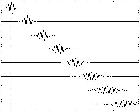
Let’s go back to our electron traveling in a more or less straight path. What’s the shape of the solution for that one? It could be anything. Well… Almost anything. As said, the only condition we can impose is that the envelope of the wave packet – its ‘general’ shape so to say – should not change. That because we should not have dispersion – as illustrated below. [Note that this illustration only represent the real or the imaginary part – not both – but you get the idea.]

dispersion

That being said, if we exclude dispersion (because a real-life electron traveling in a straight line doesn’t just disappear – as do dispersive wave packets), then, inside of that envelope, the weirdest things are possible – in theory that is. Indeed, Nature does not care much about our Fourier transforms. So the example below, which shows a theoretical wave packet (again, the real or imaginary part only) based on some theoretical distribution of the wave numbers of the (infinite number) of component waves that make up the wave packet, may or may not represent our real-life electron. However, if our electron has any resemblance to real-life, then I would expect it to not be as well-behaved as the theoretical one that’s shown below.

example of wave packet

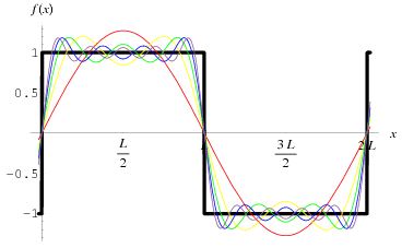
The shape above is usually referred to as a Gaussian wave packet, because of the nice normal (Gaussian) probability density functions that are associated with it. But we can also imagine a ‘square’ wave packet: a somewhat weird shape but – in terms of the math involved – as consistent as the smooth Gaussian wave packet, in the sense that we can demonstrate that the wave packet is made up of an infinite number of waves with an angular frequency ω that is linearly related to their wave number k, so the dispersion relation is ω = ak + b. [Remember we need to impose that condition to ensure that our wave packet will not dissipate (or disperse or disappear – whatever term you prefer.] That’s shown below: a Fourier analysis of a square wave.

Square wave packet

While we can construct many theoretical shapes of wave packets that respect the ‘no dispersion!’ condition, we cannot know which one will actually represent that electron we’re trying to visualize. Worse, if push comes to shove, we don’t know if these matter waves (so these wave packets) actually consist of component waves (or time-independent stationary states or whatever).

[…] OK. Let me finally admit it: while I am trying to explain you the ‘reality’ of these matter waves, we actually don’t know how real these matter waves actually are. We cannot ‘see’ or ‘touch’ them indeed. All that we know is that (i) assuming their existence, and (ii) assuming these matter waves are more or less well-behaved (e.g. that actual particles will be represented by a composite wave characterized by a linear dispersion relation between the angular frequencies and the wave numbers of its (theoretical) component waves) allows us to do all that arithmetic with these (complex-valued) probability amplitudes. More importantly, all that arithmetic with these complex numbers actually yields (real-valued) probabilities that are consistent with the probabilities we obtain through repeated experiments. So that’s what’s real and ‘not so real’ I’d say.

Indeed, the bottom-line is that we do not know what goes on inside that envelope. Worse, according to the commonly accepted Copenhagen interpretation of the Uncertainty Principle (and tons of experiments have been done to try to overthrow that interpretation – all to no avail), we never will.

Some content on this page was disabled on June 20, 2020 as a result of a DMCA takedown notice from Michael A. Gottlieb, Rudolf Pfeiffer, and The California Institute of Technology. You can learn more about the DMCA here:

https://wordpress.com/support/copyright-and-the-dmca/
Some content on this page was disabled on June 20, 2020 as a result of a DMCA takedown notice from Michael A. Gottlieb, Rudolf Pfeiffer, and The California Institute of Technology. You can learn more about the DMCA here:

https://wordpress.com/support/copyright-and-the-dmca/

End of the Road to Reality?

Pre-scriptum (dated 26 June 2020): This post did not suffer from the DMCA take-down of some material. It is, therefore, still quite readable—even if my views on these  matters have evolved quite a bit as part of my realist interpretation of QM. I now think the idea of force-carrying particles (bosons) is quite medieval. Moreover, I think the Higgs particle and other bosons (except for the photon and the neutrino) are just short-lived transients or resonances. Disequilibrium states, in other words. One should not refer to them as particles.

Original post:

Or the end of theoretical physics?

In my previous post, I mentioned the Goliath of science and engineering: the Large Hadron Collider (LHC), built by the European Organization for Nuclear Research (CERN) under the Franco-Swiss border near Geneva. I actually started uploading some pictures, but then I realized I should write a separate post about it. So here we go.

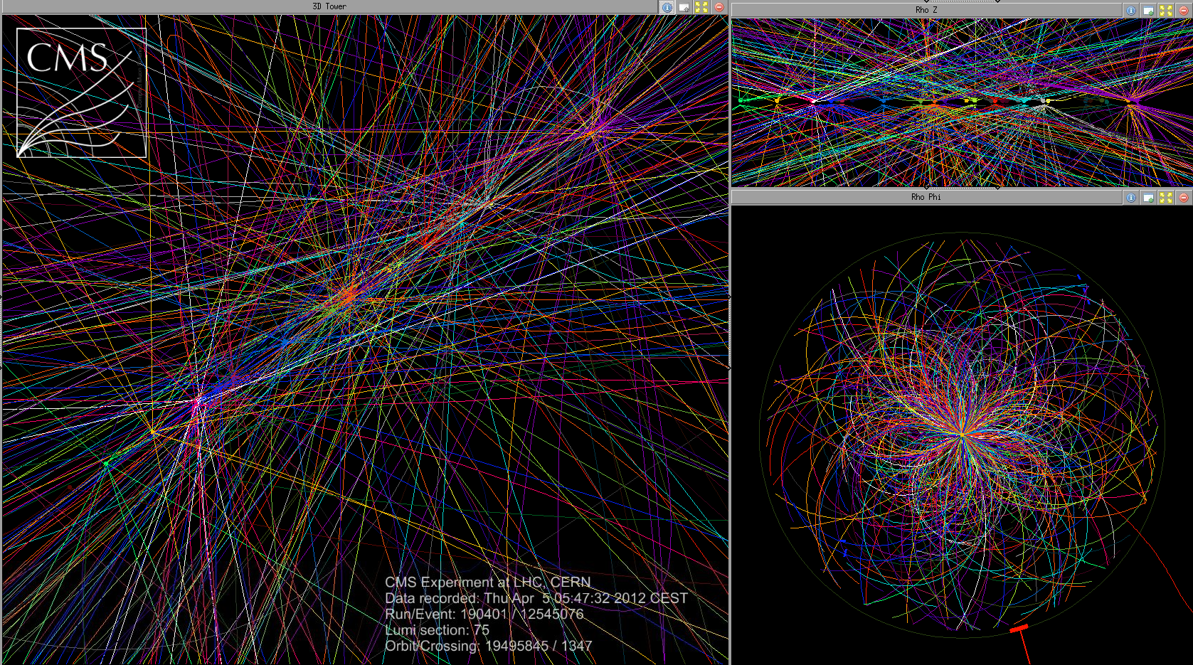
The first image (see below) shows the LHC tunnel, while the other shows (a part of) one of the two large general-purpose particle detectors that are part of this Large Hadron Collider. A detector is the thing that’s used to look at those collisions. This is actually the smallest of the two general-purpose detectors: it’s the so-called CMS detector (the other one is the ATLAS detector), and it’s ‘only’ 21.6 meter long and 15 meter in diameter – and it weighs about 12,500 tons. But so it did detect a Higgs particle – just like the ATLAS detector. [That’s actually not 100% sure but it was sure enough for the Nobel Prize committee – so I guess that should be good enough for us common mortals :-)]

LHC tunnelLHC - CMS detector

image of collision

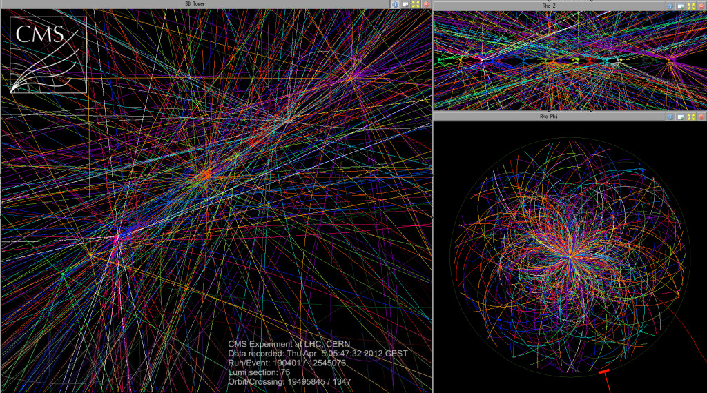
The picture above shows one of these collisions in the CMS detector. It’s not the one with the trace of the Higgs particle though. In fact, I have not found any image that actually shows the Higgs particle: the closest thing to such image are some impressionistic images on the ATLAS site. See http://atlas.ch/news/2013/higgs-into-fermions.html

In case you wonder what’s being scattered here… Well… All kinds of things – but so the original collision is usually between protons (so these are hydrogen ions: Hnuclei), although the LHC can produce other nucleon beams as well (collectively referred to as hadrons). These protons have energy levels of 4 TeV (tera-electronVolt: 1 TeV = 1000 GeV = 1 trillion eV = 1×10¹² eV).

Now, let’s think about scale once again. Remember (from that same previous post) that we calculated a wavelength of 0.33 nanometer (1 nm = 1×10⁻⁹ m, so that’s a billionth of a meter) for an electron. Well, this LHC is actually exploring the sub-femtometer (fm) frontier. One femtometer (fm) is 1×10–15 m so that’s another million times smaller. Yes: so we are talking a millionth of a billionth of a meter. The size of a proton is an estimated 1.7 femtometer indeed and, as you surely know, a proton is a point-like thing occupying a very tiny space, so it’s not like an electron ‘cloud’ swirling around: it’s much smaller. In fact, quarks – three of them make up a proton (or a neutron) – are usually thought of as being just a little bit less than half that size – so that’s about 0.7 fm.

It may also help you to use the value I mentioned for high-energy electrons when I was discussing the LEP (the Large Electron-Positron Collider, which preceded the LHC) – so that was 104.5 GeV – and calculate the associated de Broglie wavelength using E = hf and λ = v/f. The velocity is close to and, hence, if we plug everything in, we get a value close to 1.2×10⁻¹⁵ m indeed, so that’s the femtometer scale indeed. [If you don’t want to calculate anything, then just note we’re going from eV to giga-eV energy levels here, and so our wavelength decreases accordingly: one billion times smaller. Also remember (from the previous posts) that we calculated a wavelength of 0.33×10⁻⁶ m and an associated energy level of 70 eV for a slow-moving electron – i.e. one going at 2200 km per second ‘only’, i.e. less than 1% of the speed of light.]  Also note that, at these energy levels, it doesn’t matter whether or not we include the rest mass of the electron: 0.511 MeV is nothing as compared to the GeV realm. In short, we are talking very very tiny stuff here.

But so that’s the LEP scale. I wrote that the LHC is probing things at the sub-femtometer scale. So how much sub-something is that? Well… Quite a lot: the LHC is looking at stuff at a scale that’s more than a thousand times smaller. Indeed, if collision experiments in the giga-electronvolt (GeV) energy range correspond to probing stuff at the femtometer scale, then tera-electronvolt (TeV) energy levels correspond to probing stuff that’s, once again, another thousand times smaller, so we’re looking at distances of less than a thousandth of a millionth of a billionth of a meter. Now, you can try to ‘imagine’ that, but you can’t really.

So what do we actually ‘see’ then? Well… Nothing much one could say: all we can ‘see’ are traces of point-like ‘things’ being scattered, which then disintegrate or just vanish from the scene – as shown in the image above. In fact, as mentioned above, we do not even have such clear-cut ‘trace’ of a Higgs particle: we’ve got a ‘kinda signal’ only. So that’s it? Yes. But then these images are beautiful, aren’t they? If only to remind ourselves that particle physics is about more than just a bunch of formulas. It’s about… Well… The essence of reality: its intrinsic nature so to say. So… Well…

Let me be skeptical. So we know all of that now, don’t we? The so-called Standard Model has been confirmed by experiment. We now know how Nature works, don’t we? We observe light (or, to be precise, radiation: most notably that cosmic background radiation that reaches us from everywhere) that originated nearly 14 billion years ago  (to be precise: 380,000 years after the Big Bang – but what’s 380,000 years  on this scale?) and so we can ‘see’ things that are 14 billion light-years away. In fact, things that were 14 billion light-years away: indeed, because of the expansion of the universe, they are further away now and so that’s why the so-called observable universe is actually larger. So we can ‘see’ everything we need to ‘see’ at the cosmic distance scale and now we can also ‘see’ all of the particles that make up matter, i.e. quarks and electrons mainly (we also have some other so-called leptons, like neutrinos and muons), and also all of the particles that make up anti-matter of course (i.e. antiquarks, positrons etcetera). As importantly – or even more – we can also ‘see’ all of the ‘particles’ carrying the forces governing the interactions between the ‘matter particles’ – which are collectively referred to as fermions, as opposed to the ‘force carrying’ particles, which are collectively referred to as bosons (see my previous post on Bose and Fermi). Let me quickly list them – just to make sure we’re on the same page:

  1. Photons for the electromagnetic force.
  2. Gluons for the so-called strong force, which explains why positively charged protons ‘stick’ together in nuclei – in spite of their electric charge, which should push them away from each other. [You might think it’s the neutrons that ‘glue’ them together but so, no, it’s the gluons.]
  3. W+, W, and Z bosons for the so-called ‘weak’ interactions (aka as Fermi’s interaction), which explain how one type of quark can change into another, thereby explaining phenomena such as beta decay. [For example, carbon-14 will – through beta decay – spontaneously decay into nitrogen-14. Indeed, carbon-12 is the stable isotope, while carbon-14 has a life-time of 5,730 ± 40 years ‘only’ 🙂 and, hence, measuring how much carbon-14 is left in some organic substance allows us to date it (that’s what (radio)carbon-dating is about). As for the name, a beta particle can refer to an electron or a positron, so we can have β decay (e.g. the above-mentioned carbon-14 decay) as well as βdecay (e.g. magnesium-23 into sodium-23). There’s also alpha and gamma decay but that involves different things. In any case… Let me end this digression within the digression.]
  4. Finally, the existence of the Higgs particle – and, hence, of the associated Higgs field – has been predicted since 1964 already, but so it was only experimentally confirmed (i.e. we saw it, in the LHC) last year, so Peter Higgs – and a few others of course – got their well-deserved Nobel prize only 50 years later. The Higgs field gives fermions, and also the W+, W, and Z bosons, mass (but not photons and gluons, and so that’s why the weak force has such short range – as compared to the electromagnetic and strong forces).

So there we are. We know it all. Sort of. Of course, there are many questions left – so it is said. For example, the Higgs particle does actually not explain the gravitational force, so it’s not the (theoretical) graviton, and so we do not have a quantum field theory for the gravitational force. [Just Google it and you’ll see why: there’s theoretical as well as practical (experimental) reasons for that.] Secondly, while we do have a quantum field theory for all of the forces (or ‘interactions’ as physicists prefer to call them), there are a lot of constants in them (much more than just that Planck constant I introduced in my posts!) that seem to be ‘unrelated and arbitrary.’ I am obviously just quoting Wikipedia here – but it’s true.

Just look at it: three ‘generations’ of matter with various strange properties, four force fields (and some ‘gauge theory’ to provide some uniformity), bosons that have mass (the W+, W, and Z bosons, and then the Higgs particle itself) but then photons and gluons don’t… It just doesn’t look good, and then Feynman himself wrote, just a few years before his death (QED, 1985, p. 128), that the math behind calculating some of these constants (the coupling constant j for instance, or the rest mass n of an electron), which he actually invented (it makes use of a mathematical approximation method called perturbation theory) and for which he got a Nobel Prize, is a “dippy process” and that “having to resort to such hocus-pocus has prevented us from proving that the theory of quantum electrodynamics is mathematically self-consistent“. He adds: “It’s surprising that the theory still hasn’t been proved self-consistent one way or the other by now; I suspect that renormalization [“the shell game that we play to find n and j” as he calls it]  is not mathematically legitimate.” And so he writes this about quantum electrodynamics, not about “the rest of physics” (and so that’s quantum chromodynamics (QCD) – the theory of the strong interactions – and quantum flavordynamics (QFD) – the theory of weak interactions) which, he adds, “has not been checked anywhere near as well as electrodynamics.”

Waw ! That’s a pretty damning statement, isn’t it? In short, all of the celebrations around the experimental confirmation of the Higgs particle cannot hide the fact that it all looks a bit messy. There are other questions as well – most of which I don’t understand so I won’t mention them. To make a long story short, physicists and mathematicians alike seem to think there must be some ‘more fundamental’ theory behind. But – Hey! – you can’t have it all, can you? And, of course, all these theoretical physicists and mathematicians out there do need to justify their academic budget, don’t they? And so all that talk about a Grand Unification Theory (GUT) is probably just what is it: talk. Isn’t it? Maybe.

The key question is probably easy to formulate: what’s beyond this scale of a thousandth of a proton diameter (0.001×10⁻¹⁵ m) – a thousandth of a millionth of a billionth of a meter that is. Well… Let’s first note that this so-called ‘beyond’ is a ‘universe’ which mankind (or let’s just say ‘we’) will never see. Never ever. Why? Because there is no way to go substantially beyond the 4 TeV energy levels that were reached last year – at great cost – in the world’s largest particle collider (the LHC). Indeed, the LHC is widely regarded not only as “the most complex and ambitious scientific project ever accomplished by humanity” (I am quoting a CERN scientist here) but – with a cost of more than 7.5 billion Euro – also as one of the most expensive ones. Indeed, taking into account inflation and all that, it was like the Manhattan project indeed (although scientists loathe that comparison). So we should not have any illusions: there will be no new super-duper LHC any time soon, and surely not during our lifetime: the current LHC is the super-duper thing!

Indeed, when I write ‘substantially‘ above, I really mean substantially. Just to put things in perspective: the LHC is currently being upgraded to produce 7 TeV beams (it was shut down for this upgrade, and it should come back on stream in 2015). That sounds like an awful lot (from 4 to 7 is +75%), and it is: it amounts to packing the kinetic energy of seven flying mosquitos (instead of four previously :-)) into each and every particle that makes up the beam. But that’s not substantial, in the sense that it is very much below the so-called GUT energy scale, which is the energy level above which, it is believed (by all those GUT theorists at least), the electromagnetic force, the weak force and the strong force will all be part and parcel of one and the same unified force. Don’t ask me why (I’ll know when I finished reading Penrose, I hope) but that’s what it is (if I should believe what I am reading currently that is). In any case, the thing to remember is that the GUT energy levels are in the 1016 GeV range, so that’s – sorry for all these numbers – a trillion TeV. That amounts to pumping more than 160,000 Joule in each of those tiny point-like particles that make up our beam. So… No. Don’t even try to dream about it. It won’t happen. That’s science fiction – with the emphasis on fiction. [Also don’t dream about a trillion flying mosquitos packed into one proton-sized super-mosquito either. :-)]

So what?

Well… I don’t know. Physicists refer to the zone beyond the above-mentioned scale (so things smaller than 0.001×10⁻¹⁵ m) as the Great Desert. That’s a very appropriate name I think – for more than one reason. And so it’s this ‘desert’ that Roger Penrose is actually trying to explore in his ‘Road to Reality’. As for me, well… I must admit I have great trouble following Penrose on this road. I’ve actually started to doubt that Penrose’s Road leads to Reality. Maybe it takes us away from it. Huh? Well… I mean… Perhaps the road just stops at that 0.001×10⁻¹⁵ m frontier? 

In fact, that’s a view which one of the early physicists specialized in high-energy physics, Raoul Gatto, referred to as the zeroth scenarioI am actually not quoting Gatto here, but another theoretical physicist: Gerard ‘t Hooft, another Nobel prize winner (you may know him better because he’s a rather fervent Mars One supporter, but so here I am referring to his popular 1996 book In Search of the Ultimate Building Blocks). In any case, Gatto, and most other physicists, including ‘T Hooft (despite the fact ‘T Hooft got his Nobel prize for his contribution to gauge theory – which, together with Feynman’s application of perturbation theory to QED, is actually the backbone of the Standard Model) firmly reject this zeroth scenario. ‘T Hooft himself thinks superstring theory (i.e. supersymmetric string theory – which has now been folded into M-theory or – back to the original term – just string theory – the terminology is quite confusing) holds the key to exploring this desert.

But who knows? In fact, we can’t – because of the above-mentioned practical problem of experimental confirmation. So I am likely to stay on this side of the frontier for quite a while – if only because there’s still so much to see here and, of course, also because I am just at the beginning of this road. 🙂 And then I also realize I’ll need to understand gauge theory and all that to continue on this road – which is likely to take me another six months or so (if not more) and then, only then, I might try to look at those little strings, even if we’ll never see them because… Well… Their theoretical diameter is the so-called Planck length. So what? Well… That’s equal to 1.6×10⁻³⁵ m. So what? Well… Nothing. It’s just that 1.6×10⁻³⁵ m is 1/10 000 000 000 000 000 of that sub-femtometer scale. I don’t even want to write this in trillionths of trillionths of trillionths etcetera because I feel that’s just not making any sense. And perhaps it doesn’t. One thing is for sure: that ‘desert’ that GUT theorists want us to cross is not just ‘Great’: it’s ENORMOUS!

Richard Feynman – another Nobel Prize scientist whom I obviously respect a lot – surely thought trying to cross a desert like that amounts to certain death. Indeed, he’s supposed to have said the following about string theorists, about a year or two before he died (way too young): I don’t like that they’re not calculating anything. I don’t like that they don’t check their ideas. I don’t like that for anything that disagrees with an experiment, they cook up an explanation–a fix-up to say, “Well, it might be true.” For example, the theory requires ten dimensions. Well, maybe there’s a way of wrapping up six of the dimensions. Yes, that’s all possible mathematically, but why not seven? When they write their equation, the equation should decide how many of these things get wrapped up, not the desire to agree with experiment. In other words, there’s no reason whatsoever in superstring theory that it isn’t eight out of the ten dimensions that get wrapped up and that the result is only two dimensions, which would be completely in disagreement with experience. So the fact that it might disagree with experience is very tenuous, it doesn’t produce anything; it has to be excused most of the time. It doesn’t look right.”

Hmm…  Feynman and ‘T Hooft… Two giants in science. Two Nobel Prize winners – and for stuff that truly revolutionized physics. The amazing thing is that those two giants – who are clearly at loggerheads on this one – actually worked closely together on a number of other topics – most notably on the so-called Feynman-‘T Hooft gauge, which – as far as I understand – is the one that is most widely used in quantum field calculations. But I’ll leave it at that here – and I’ll just make a mental note of the terminology here. The Great Desert… Probably an appropriate term. ‘T Hooft says that most physicists think that desert is full of tiny flowers. I am not so sure – but then I am not half as smart as ‘T Hooft. Much less actually. So I’ll just see where the road I am currently following leads me. With Feynman’s warning in mind, I should probably expect the road condition to deteriorate quickly.

Post scriptum: You will not be surprised to hear that there’s a word for 1×10–18 m: it’s called an attometer (with two t’s, and abbreviated as am). And beyond that we have zeptometer (1 zm = 1×10–21 m) and yoctometer (1 ym = 1×10–23 m). In fact, these measures actually represent something: 20 yoctometer is the estimated radius of a 1 MeV neutrino – or, to be precise, its the radius of the cross section, which is “the effective area that governs the probability of some scattering or absorption event.” But so then there are no words anymore. The next measure is the Planck length: 1.62 × 10⁻³⁵ m – but so that’s a trillion (1012) times smaller than a yoctometer. Unimaginable, isn’t it? Literally. 

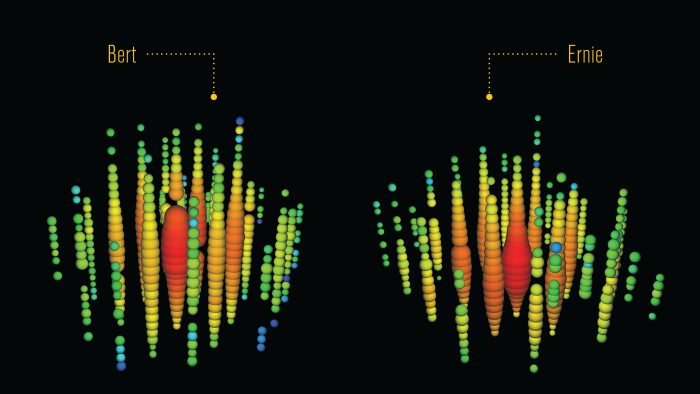
Note: A 1 MeV neutrino? Well… Yes. The estimated rest mass of an (electron) neutrino is tiny: at least 50,000 times smaller than the mass of the electron and, therefore, neutrinos are often assumed to be massless, for all practical purposes that is. However, just like the massless photon, they can carry high energy. High-energy gamma ray photons, for example, are also associated with MeV energy levels. Neutrinos are one of the many particles produced in high-energy particle collisions in particle accelerators, but they are present everywhere: they’re produced by stars (which, as you know, are nuclear fusion reactors). In fact, most neutrinos passing through Earth are produced by our Sun. The largest neutrino detector on Earth is called IceCube. It sits on the South Pole – or under it, as it’s suspended under the Antarctic ice, and it regularly captures high-energy neutrinos in the range of 1 to 10 TeV. Last year (in November 2013), it captured two with energy levels around 1000 TeV – so that’s the peta-electronvolt level (1 PeV = 1×10¹⁵ eV). If you think that’s amazing, it is. But also remember that 1 eV is 1.6×10⁻¹⁹ Joule, so it’s ‘only’ a ten-thousandth of a Joule. In other words, you would need at least ten thousand of them to briefly light up an LED. The PeV pair was dubbed Bert and Ernie and the illustration below (from IceCube’s website) conveys how the detectors sort of lit up when they passed. It was obviously a pretty clear ‘signal’ – but so the illustration also makes it clear that we don’t really ‘see’ at such small scale: we just know ‘something’ happened.

Bert and Ernie

The Uncertainty Principle re-visited: Fourier transforms and conjugate variables

Pre-scriptum (dated 26 June 2020): This post did not suffer from the DMCA take-down of some material. It is, therefore, still quite readable—even if my views on the nature of the Uncertainty Principle have evolved quite a bit as part of my realist interpretation of QM.

Original post:

In previous posts, I presented a time-independent wave function for a particle (or wavicle as we should call it – but so that’s not the convention in physics) – let’s say an electron – traveling through space without any external forces (or force fields) acting upon it. So it’s just going in some random direction with some random velocity v and, hence, its momentum is p = mv. Let me be specific – so I’ll work with some numbers here – because I want to introduce some issues related to units for measurement.

So the momentum of this electron is the product of its mass m (about 9.1×10⁻²⁸ grams) with its velocity v (typically something in the range around 2,200 km/s, which is fast but not even close to the speed of light – and, hence, we don’t need to worry about relativistic effects on its mass here). Hence, the momentum p of this electron would be some 20×10−25 kg·m/s. Huh? Kg·m/s?Well… Yes, kg·m/s or N·s are the usual measures of momentum in classical mechanics: its dimension is [mass][length]/[time] indeed. However, you know that, in atomic physics, we don’t want to work with these enormous units (because we then always have to add these ×10−28 and ×10−25 factors and so that’s a bit of a nuisance indeed). So the momentum p will usually be measured in eV/c, with c representing what it usually represents, i.e. the speed of light. Huh? What’s this strange unit? Electronvolts divided by c? Well… We know that eV is an appropriate unit for measuring energy in atomic physics: we can express eV in Joule and vice versa: 1 eV = 1.6×10⁻¹⁹ Joule, so that’s OK – except for the fact that this Joule is a monstrously large unit at the atomic scale indeed, and so that’s why we prefer electronvolt. But the Joule is a shorthand unit for kg·m2/s2, which is the measure for energy expressed in SI units, so there we are: while the SI dimension for energy is actually [mass][length]2/[time]2, using electronvolts (eV) is fine. Now, just divide the SI dimension for energy, i.e. [mass][length]2/[time]2, by the SI dimension for velocity, i.e. [length]/[time]: we get something expressed in [mass][length]/[time]. So that’s the SI dimension for momentum indeed! In other words, dividing some quantity expressed in some measure for energy (be it Joules or electronvolts or erg or calories or coulomb-volts or BTUs or whatever – there’s quite a lot of ways to measure energy indeed!) by the speed of light (c) will result in some quantity with the right dimensions indeed. So don’t worry about it. Now, 1 eV/c is equivalent to 5.344×10⁻²⁸ kg·m/s, so the momentum of this electron will be 3.75 eV/c.

Let’s go back to the main story now. Just note that the momentum of this electron that we are looking at is a very tiny amount – as we would expect of course.

Time-independent means that we keep the time variable (t) in the wave function Ψ(x, t) fixed and so we only look at how Ψ(x, t) varies in space, with x as the (real) space variable representing position. So we have a simplified wave function Ψ(x) here: we can always put the time variable back in when we’re finished with the analysis. By now, it should also be clear that we should distinguish between real-valued wave functions and complex-valued wave functions. Real-valued wave functions represent what Feynman calls “real waves”, like a sound wave, or an oscillating electromagnetic field. Complex-valued wave functions describe probability amplitudes. They are… Well… Feynman actually stops short of saying that they are not real. So what are they?

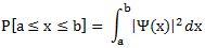
They are, first and foremost complex numbers, so they have a real and a so-called imaginary part (z = a + ib or, if we use polar coordinates, reθ = cosθ + isinθ). Now, you may think – and you’re probably right to some extent – that the distinction between ‘real’ waves and ‘complex’ waves is, perhaps, less of a dichotomy than popular writers – like me 🙂 – suggest. When describing electromagnetic waves, for example, we need to keep track of both the electric field vector E as well as the magnetic field vector B (both are obviously related through Maxwell’s equations). So we have two components as well, so to say, and each of these components has three dimensions in space, and we’ll use the same mathematical tools to describe them (so we will also represent them using complex numbers). That being said, these probability amplitudes usually denoted by Ψ(x), describe something very different. What exactly? Well… By now, it should be clear that that is actually hard to explain: the best thing we can do is to work with them, so they start feeling familiar. The main thing to remember is that we need to square their modulus (or magnitude or absolute value if you find these terms more comprehensible) to get a probability (P). For example, the expression below gives the probability of finding a particle – our electron for example – in in the (space) interval [a, b]:

probability versus amplitude

Of course, we should not be talking intervals but three-dimensional regions in space. However, we’ll keep it simple: just remember that the analysis should be extended to three (space) dimensions (and, of course, include the time dimension as well) when we’re finished (to do that, we’d use so-called four-vectors – another wonderful mathematical invention).

Now, we also used a simple functional form for this wave function, as an example: Ψ(x) could be proportional, we said, to some idealized function eikx. So we can write: Ψ(x) ∝ eikx (∝ is the standard symbol expressing proportionality). In this function, we have a wave number k, which is like the frequency in space of the wave (but then measured in radians because the phase of the wave function has to be expressed in radians). In fact, we actually wrote Ψ(x, t) = (1/x)ei(kx – ωt) (so the magnitude of this amplitude decreases with distance) but, again, let’s keep it simple for the moment: even with this very simple function eikx , things will become complex enough.

We also introduced the de Broglie relation, which gives this wave number k as a function of the momentum p of the particle: k = p/ħ, with ħ the (reduced) Planck constant, i.e. a very tiny number in the neighborhood of 6.582 ×10⁻¹⁶ eV·s. So, using the numbers above, we’d have a value for k equal to 3.75 eV/c divided by 6.582 ×10⁻¹⁶ eV·s. So that’s 0.57×10¹⁶ (radians) per… Hey, how do we do it with the units here? We get an incredibly huge number here (57 with 14 zeroes after it) per second? We should get some number per meter because k is expressed in radians per unit distance, right? Right. We forgot c. We are actually measuring distance here, but in light-seconds instead of meter: k is 0.57×10¹⁶/s. Indeed, a light-second is the distance traveled by light in one second, so that’s s, and if we want k expressed in radians per meter, then we need to divide this huge number 0.57×10¹⁶ (in rad) by 2.998×10⁸ ( in (m/s)·s) and so then we get a much more reasonable value for k, and with the right dimension too: to be precise, k is about 19×106 rad/m in this case. That’s still huge: it corresponds with a wavelength of 0.33 nanometer (1 nm = 10-6 m) but that’s the correct order of magnitude indeed.

[In case you wonder what formula I am using to calculate the wavelength: it’s λ = 2π/k. Note that our electron’s wavelength is more than a thousand times shorter than the wavelength of (visible) light (we humans can see light with wavelengths ranging from 380 to 750 nm) but so that’s what gives the electron its particle-like character! If we would increase their velocity (e.g. by accelerating them in an accelerator, using electromagnetic fields to propel them to speeds closer to and also to contain them in a beam), then we get hard beta rays. Hard beta rays are surely not as harmful as high-energy electromagnetic rays. X-rays and gamma rays consist of photons with wavelengths ranging from 1 to 100 picometer (1 pm = 10–12 m) – so that’s another factor of a thousand down – and thick lead shields are needed to stop them: they are the cause of cancer (Marie Curie’s cause of death), and the hard radiation of a nuclear blast will always end up killing more people than the immediate blast effect. In contrast, hard beta rays will cause skin damage (radiation burns) but they won’t go deeper than that.]

Let’s get back to our wave function Ψ(x) ∝ eikx. When we introduced it in our previous posts, we said it could not accurately describe a particle because this wave function (Ψ(x) = Aeikx) is associated with probabilities |Ψ(x)|2 that are the same everywhere. Indeed,  |Ψ(x)|2 = |Aeikx|2 = A2. Apart from the fact that these probabilities would add up to infinity (so this mathematical shape is unacceptable anyway), it also implies that we cannot locate our electron somewhere in space. It’s everywhere and that’s the same as saying it’s actually nowhere. So, while we can use this wave function to explain and illustrate a lot of stuff (first and foremost the de Broglie relations), we actually need something different if we would want to describe anything real (which, in the end, is what physicists want to do, right?). We already said in our previous posts: real particles will actually be represented by a wave packet, or a wave train. A wave train can be analyzed as a composite wave consisting of a (potentially infinite) number of component waves. So we write:

Composite wave

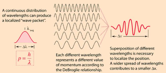
Note that we do not have one unique wave number k or – what amounts to saying the same – one unique value p for the momentum: we have n values. So we’re introducing a spread in the wavelength here, as illustrated below:

Explanation of uncertainty principle

In fact, the illustration above talks of a continuous distribution of wavelengths and so let’s take the continuum limit of the function above indeed and write what we should be writing:

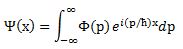
Composite wave - integral

Now that is an interesting formula. [Note that I didn’t care about normalization issues here, so it’s not quite what you’d see in a more rigorous treatment of the matter. I’ll correct that in the Post Scriptum.] Indeed, it shows how we can get the wave function Ψ(x) from some other function Φ(p). We actually encountered that function already, and we referred to it as the wave function in the momentum space. Indeed, Nature does not care much what we measure: whether it’s position (x) or momentum (p), Nature will not share her secrets with us and, hence, the best we can do – according to quantum mechanics – is to find some wave function associating some (complex) probability amplitude with each and every possible (real) value of x or p. What the equation above shows, then, is these wave functions come as a pair: if we have Φ(p), then we can calculate Ψ(x) – and vice versa. Indeed, the particular relation between Ψ(x) and Φ(p) as established above, makes Ψ(x) and Φ(p) a so-called Fourier transform pair, as we can transform Φ(p) into Ψ(x) using the above Fourier transform (that’s how that  integral is called), and vice versa. More in general, a Fourier transform pair can be written as:

Fourier transform pair

Instead of x and p, and Ψ(x) and Φ(p), we have x and y, and f(x) and g(y), in the formulas above, but so that does not make much of a difference when it comes to the interpretation: x and p (or x and y in the formulas above) are said to be conjugate variables. What it means really is that they are not independent. There are quite a few of such conjugate variables in quantum mechanics such as, for example: (1) time and energy (and time and frequency, of course, in light of the de Broglie relation between both), and (2) angular momentum and angular position (or orientation). There are other pairs too but these involve quantum-mechanical variables which I do not understand as yet and, hence, I won’t mention them here. [To be complete, I should also say something about that 1/2π factor, but so that’s just something that pops up when deriving the Fourier transform from the (discrete) Fourier series on which it is based. We can put it in front of either integral, or split that factor across both. Also note the minus sign in the exponent of the inverse transform.]

When you look at the equations above, you may think that f(x) and g(y) must be real-valued functions. Well… No. The Fourier transform can be used for both real-valued as well as complex-valued functions. However, at this point I’ll have to refer those who want to know each and every detail about these Fourier transforms to a course in complex analysis (such as Brown and Churchill’s Complex Variables and Applications (2004) for instance) or, else, to a proper course on real and complex Fourier transforms (they are used in signal processing – a very popular topic in engineering – and so there’s quite a few of those courses around).

The point to note in this post is that we can derive the Uncertainty Principle from the equations above. Indeed, the (complex-valued) functions Ψ(x) and Φ(p) describe (probability) amplitudes, but the (real-valued) functions |Ψ(x)|2 and |Φ(p)|2 describe probabilities or – to be fully correct – they are probability (density) functions. So it is pretty obvious that, if the functions Ψ(x) and Φ(p) are a Fourier transform pair, then |Ψ(x)|2 and |Φ(p)|2 must be related to. They are. The derivation is a bit lengthy (and, hence, I will not copy it from the Wikipedia article on the Uncertainty Principle) but one can indeed derive the so-called Kennard formulation of the Uncertainty Principle from the above Fourier transforms. This Kennard formulation does not use this rather vague Δx and Δp symbols but clearly states that the product of the standard deviation from the mean of these two probability density functions can never be smaller than ħ/2:

σxσ≥ ħ/2

To be sure: ħ/2 is a rather tiny value, as you should know by now, 🙂 but, so, well… There it is.

As said, it’s a bit lengthy but not that difficult to do that derivation. However, just for once, I think I should try to keep my post somewhat shorter than usual so, to conclude, I’ll just insert one more illustration here (yes, you’ve seen that one before), which should now be very easy to understand: if the wave function Ψ(x) is such that there’s relatively little uncertainty about the position x of our electron, then the uncertainty about its momentum will be huge (see the top graphs). Vice versa (see the bottom graphs), precise information (or a narrow range) on its momentum, implies that its position cannot be known.

2000px-Quantum_mechanics_travelling_wavefunctions_wavelength

Does all this math make it any easier to understand what’s going on? Well… Yes and no, I guess. But then, if even Feynman admits that he himself “does not understand it the way he would like to” (Feynman Lectures, Vol. III, 1-1), who am I? In fact, I should probably not even try to explain it, should I? 🙂

So the best we can do is try to familiarize ourselves with the language used, and so that’s math for all practical purposes. And, then, when everything is said and done, we should probably just contemplate Mario Livio’s question: Is God a mathematician? 🙂

Post scriptum:

I obviously cut corners above, and so you may wonder how that ħ factor can be related to σand σ if it doesn’t appear in the wave functions. Truth be told, it does. Because of (i) the presence of ħ in the exponent in our ei(p/ħ)x function, (ii) normalization issues (remember that probabilities (i.e. Ψ|(x)|2 and |Φ(p)|2) have to add up to 1) and, last but not least, (iii) the 1/2π factor involved in Fourier transforms , Ψ(x) and Φ(p) have to be written as follows:

Position and momentum wave functionNote that we’ve also re-inserted the time variable here, so it’s pretty complete now. One more thing we could do is to substitute x for a proper three-dimensional space vector or, better still, introduce four-vectors, which would allow us to also integrate relativistic effects (most notably the slowing of time with motion – as observed from the stationary reference frame) – which become important when, for instance, we’re looking at electrons being accelerated, which is the rule, rather than the exception, in experiments.

Remember (from a previous post) that we calculated that an electron traveling at its usual speed in orbit (2200 km/s, i.e. less than 1% of the speed of light) had an energy of about 70 eV? Well, the Large Electron-Positron Collider (LEP) did accelerate them to speeds close to light, thereby giving them energy levels topping 104.5 billion eV (or 104.5 GeV as it’s written) so they could hit each other with collision energies topping 209 GeV (they come from opposite directions so it’s two times 104.5 GeV). Now, 209 GeV is tiny when converted to everyday energy units: 209 GeV is 33×10–9 Joule only indeed – and so note the minus sign in the exponent here: we’re talking billionths of a Joule here. Just to put things into perspective: 1 Watt is the energy consumption of an LED (and 1 Watt is 1 Joule per second), so you’d need to combine the energy of billions of these fast-traveling electrons to power just one little LED lamp. But, of course, that’s not the right comparison: 104.5 GeV is more than 200,000 times the electron’s rest mass (0.511 MeV), so that means that – in practical terms – their mass (remember that mass is a measure for inertia) increased by the same factor (204,500 times to be precise). Just to give an idea of the effort that was needed to do this: CERN’s LEP collider was housed in a tunnel with a circumference of 27 km. Was? Yes. The tunnel is still there but it now houses the Large Hadron Collider (LHC) which, as you surely know, is the world’s largest and most powerful particle accelerator: its experiments confirmed the existence of the Higgs particle in 2013, thereby confirming the so-called Standard Model of particle physics. [But I’ll see a few things about that in my next post.]

Oh… And, finally, in case you’d wonder where we get the inequality sign in σxσ≥ ħ/2, that’s because – at some point in the derivation – one has to use the Cauchy-Schwarz inequality (aka as the triangle inequality): |z1+ z1| ≤ |z1|+| z1|. In fact, to be fully complete, the derivation uses the more general formulation of the Cauchy-Schwarz inequality, which also applies to functions as we interpret them as vectors in a function space. But I would end up copying the whole derivation here if I add any more to this – and I said I wouldn’t do that. 🙂 […]

An easy piece: introducing quantum mechanics and the wave function

Pre-scriptum (dated 26 June 2020): A quick glance at this piece – so many years after I have written it – tells me it is basically OK. However, it is quite obvious that, in terms of interpreting the math, I have come a very long way. However, I would recommend you go through the piece so as to get the basic math, indeed, and then you may or may not be ready for the full development of my realist or classical interpretation of QM. My manuscript may also be a fun read for you.

Original post:

After all those boring pieces on math, it is about time I got back to physics. Indeed, what’s all that stuff on differential equations and complex numbers good for? This blog was supposed to be a journey into physics, wasn’t it? Yes. But wave functions – functions describing physical waves (in classical mechanics) or probability amplitudes (in quantum mechanics) – are the solution to some differential equation, and they will usually involve complex-number notation. However, I agree we have had enough of that now. Let’s see how it works. By the way, the title of this post – An Easy Piece – is an obvious reference to (some of) Feynman’s 1965 Lectures on Physics, some of which were re-packaged in 1994 (six years after his death that is) in ‘Six Easy Pieces’ indeed – but, IMHO, it makes more sense to read all of them as part of the whole series.

Let’s first look at one of the most used mathematical shapes: the sinusoidal wave. The illustration below shows the basic concepts: we have a wave here – some kind of cyclic thing – with a wavelength λ, an amplitude (or height) of (maximum) A0, and a so-called phase shift equal to φ. The Wikipedia definition of a wave is the following: “a wave is a disturbance or oscillation that travels through space and matter, accompanied by a transfer of energy.” Indeed, a wave transports energy as it travels (oh – I forgot to mention the speed or velocity of a wave (v) as an important characteristic of a wave), and the energy it carries is directly proportional to the square of the amplitude of the wave: E ∝ A2 (this is true not only for waves like water waves, but also for electromagnetic waves, like light).

Cosine wave concepts

Let’s now look at how these variables get into the argument – literally: into the argument of the wave function. Let’s start with that phase shift. The phase shift is usually defined referring to some other wave or reference point (in this case the origin of the x and y axis). Indeed, the amplitude – or ‘height’ if you want (think of a water wave, or the strength of the electric field) – of the wave above depends on (1) the time t (not shown above) and (2) the location (x), but so we will need to have this phase shift φ in the argument of the wave function because at x = 0 we do not have a zero height for the wave. So, as we can see, we can shift the x-axis left or right with this φ. OK. That’s simple enough. Let’s look at the other independent variables now: time and position.

The height (or amplitude) of the wave will obviously vary both in time as well as in space. On this graph, we fixed time (t = 0) – and so it does not appear as a variable on the graph – and show how the amplitude y = A varies in space (i.e. along the x-axis). We could also have looked at one location only (x = 0 or x1 or whatever other location) and shown how the amplitude varies over time at that location only. The graph would be very similar, except that we would have a ‘time distance’ between two crests (or between two troughs or between any other two points separated by a full cycle of the wave) instead of the wavelength λ (i.e. a distance in space). This ‘time distance’ is the time needed to complete one cycle and is referred to as the period of the wave (usually denoted by the symbol T or T– in line with the notation for the maximum amplitude A0). In other words, we will also see time (t) as well as location (x) in the argument of this cosine or sine wave function. By the way, it is worth noting that it does not matter if we use a sine or cosine function because we can go from one to the other using the basic trigonometric identities cos θ = sin(π/2 – θ) and sin θ = cos(π/2 – θ). So all waves of the shape above are referred to as sinusoidal waves even if, in most cases, the convention is to actually use the cosine function to represent them.

So we will have x, t and φ in the argument of the wave function. Hence, we can write A = A(x, t, φ) = cos(x + t + φ) and there we are, right? Well… No. We’re adding very different units here: time is measured in seconds, distance in meter, and the phase shift is measured in radians (i.e. the unit of choice for angles). So we can’t just add them up. The argument of a trigonometric function (like this cosine function) is an angle and, hence, we need to get everything in radians – because that’s the unit we use to measure angles. So how do we do that? Let’s do it step by step.

First, it is worth noting that waves are usually caused by something. For example, electromagnetic waves are caused by an oscillating point charge somewhere, and radiate out from there. Physical waves – like water waves, or an oscillating string – usually also have some origin. In fact, we can look at a wave as a way of transmitting energy originating elsewhere. In the case at hand here – i.e. the nice regular sinusoidal wave illustrated above – it is obvious that the amplitude at some time t = tat some point x = x1 will be the same as the amplitude of that wave at point x = 0 some time ago. How much time ago? Well… The time (t) that was needed for that wave to travel from point x = 0 to point x = xis easy to calculate: indeed, if the wave originated at t = 0 and x = 0, then x1 (i.e. the distance traveled by the wave) will be equal to its velocity (v) multiplied by t1, so we have x1= v.t1 (note that we assume the wave velocity is constant – which is a very reasonable assumption). In other words, inserting x1and t1 in the argument of our cosine function should yield the same value as inserting zero for x and t. Distance and time can be substituted so to say, and that’s we will have something like x – vt or vt – x in the argument in that cosine function: we measure both time and distance in units of distance so to say. [Note that x – vt and –(x-vt) = vt – x are equivalent because cos θ = cos (-θ)]

Does this sound fishy? It shouldn’t. Think about it. In the (electric) field equation for electromagnetic radiation (that’s one of the examples of a wave which I mentioned above), you’ll find the so-called retarded acceleration a(t – x/c) in the argument: that’s the acceleration (a)of the charge causing the electric field at point x to change not at time t but at time t – x/c. So that’s the retarded acceleration indeed: x/c is the time it took for the wave to travel from its origin (the oscillating point charge) to x and so we subtract that from t. [When talking electromagnetic radiation (e.g. light), the wave velocity v is obviously equal to c, i.e. the speed of light, or of electromagnetic radiation in general.] Of course, you will now object that t – x/c is not the same as vt – x, and you are right: we need time units in the argument of that acceleration function, not distance. We can get to distance units if we would multiply the time with the wave velocity v but that’s complicated business because the velocity of that moving point charge is not a constant.

[…] I am not sure if I made myself clear here. If not, so be it. The thing to remember is that we need an input expressed in radians for our cosine function, not time, nor distance. Indeed, the argument in a sine or cosine function is an angle, not some distance. We will call that angle the phase of the wave, and it is usually denoted by the symbol θ  – which we also used above. But so far we have been talking about amplitude as a function of distance, and we expressed time in distance units too – by multiplying it with v. How can we go from some distance to some angle? It is simple: we’ll multiply x – vt with 2π/λ.

Huh? Yes. Think about it. The wavelength will be expressed in units of distance – typically 1 m in the SI International System of Units but it could also be angstrom (10–10 m = 0.1 nm) or nano-meter (10–9 m = 10 Å). A wavelength of two meter (2 m) means that the wave only completes half a cycle per meter of travel. So we need to translate that into radians, which – once again – is the measure used to… well… measure angles, or the phase of the wave as we call it here. So what’s the ‘unit’ here? Well… Remember that we can add or subtract 2π (and any multiple of 2π, i.e. ± 2nπ with n = ±1, ±2, ±3,…) to the argument of all trigonometric functions and we’ll get the same value as for the original argument. In other words, a cycle characterized by a wavelength λ corresponds to the angle θ going around the origin and describing one full circle, i.e. 2π radians. Hence, it is easy: we can go from distance to radians by multiplying our ‘distance argument’ x – vt with 2π/λ. If you’re not convinced, just work it out for the example I gave: if the wavelength is 2 m, then 2π/λ equals 2π/2 = π. So traveling 6 meters along the wave – i.e. we’re letting x go from 0 to 6 m while fixing our time variable – corresponds to our phase θ going from 0 to 6π: both the ‘distance argument’ as well as the change in phase cover three cycles (three times two meter for the distance, and three times 2π for the change in phase) and so we’re fine. [Another way to think about it is to remember that the circumference of the unit circle is also equal to 2π (2π·r = 2π·1 in this case), so the ratio of 2π to λ measures how many times the circumference contains the wavelength.]

In short, if we put time and distance in the (2π/λ)(x-vt) formula, we’ll get everything in radians and that’s what we need for the argument for our cosine function. So our sinusoidal wave above can be represented by the following cosine function:

A = A(x, t) = A0cos[(2π/λ)(x-vt)]

We could also write A = A0cosθ with θ = (2π/λ)(x-vt). […] Both representations look rather ugly, don’t they? They do. And it’s not only ugly: it’s not the standard representation of a sinusoidal wave either. In order to make it look ‘nice’, we have to introduce some more concepts here, notably the angular frequency and the wave number. So let’s do that.

The angular frequency is just like the… well… the frequency you’re used to, i.e. the ‘non-angular’ frequency f,  as measured in cycles per second (i.e. in Hertz). However, instead of measuring change in cycles per second, the angular frequency (usually denoted by the symbol ω) will measure the rate of change of the phase with time, so we can write or define ω as ω = ∂θ/∂t. In this case, we can easily see that ω = –2πv/λ. [Note that we’ll take the absolute value of that derivative because we want to work with positive numbers for such properties of functions.] Does that look complicated? In doubt, just remember that ω is measured in radians per second and then you can probably better imagine what it is really. Another way to understand ω somewhat better is to remember that the product of ω and the period T is equal to 2π, so that’s a full cycle. Indeed, the time needed to complete one cycle multiplied with the phase change per second (i.e. per unit time) is equivalent to going round the full circle: 2π = ω.T. Because f = 1/T, we can also relate ω to f and write ω = 2π.f = 2π/T.

Likewise, we can measure the rate of change of the phase with distance, and that gives us the wave number k = ∂θ/∂x, which is like the spatial frequency of the wave. So it is just like the wavelength but then measured in radians per unit distance. From the function above, it is easy to see that k = 2π/λ. The interpretation of this equality is similar to the ω.T = 2π equality. Indeed, we have a similar equation for k: 2π = k.λ, so the wavelength (λ) is for k what the period (T) is for ω. If you’re still uncomfortable with it, just play a bit with some numerical examples and you’ll be fine.

To make a long story short, this, then, allows us to re-write the sinusoidal wave equation above in its final form (and let me include the phase shift φ again in order to be as complete as possible at this stage):

A(x, t) = A0cos(kx – ωt + φ)

You will agree that this looks much ‘nicer’ – and also more in line with what you’ll find in textbooks or on Wikipedia. 🙂 I should note, however, that we’re not adding any new parameters here. The wave number k and the angular frequency ω are not independent: this is still the same wave (A = A0cos[(2π/λ)(x-vt)]), and so we are not introducing anything more than the frequency and – equally important – the speed with which the wave travels, which is usually referred to as the phase velocity. In fact, it is quite obvious from the ω.T = 2π and the k = 2π/λ identities that kλ = ω.T and, hence, taking into account that λ is obviously equal to λ = v.T (the wavelength is – by definition – the distance traveled by the wave in one period), we find that the phase (or wave) velocity v is equal to the ratio of ω and k, so we have that v = ω/k. So x, t, ω and k could be re-scaled or so but their ratio cannot change: the velocity of the wave is what it is. In short, I am introducing two new concepts and symbols (ω and k) but there are no new degrees of freedom in the system so to speak.

[At this point, I should probably say something about the difference between the phase velocity and the so-called group velocity of a wave. Let me do that in as brief a way as I can manage. Most real-life waves travel as a wave packet, aka a wave train. So that’s like a burst, or an “envelope” (I am shamelessly quoting Wikipedia here…), of “localized wave action that travels as a unit.” Such wave packet has no single wave number or wavelength: it actually consists of a (large) set of waves with phases and amplitudes such that they interfere constructively only over a small region of space, and destructively elsewhere. The famous Fourier analysis (or infamous if you have problems understanding what it is really) decomposes this wave train in simpler pieces. While these ‘simpler’ pieces – which, together, add up to form the wave train – are all ‘nice’ sinusoidal waves (that’s why I call them ‘simple’), the wave packet as such is not. In any case (I can’t be too long on this), the speed with which this wave train itself is traveling through space is referred to as the group velocity. The phase velocity and the group velocity are usually very different: for example, a wave packet may be traveling forward (i.e. its group velocity is positive) but the phase velocity may be negative, i.e. traveling backward. However, I will stop here and refer to the Wikipedia article on group and phase velocity: it has wonderful illustrations which are much and much better than anything I could write here. Just one last point that I’ll use later: regardless of the shape of the wave (sinusoidal, sawtooth or whatever), we have a very obvious relationship relating wavelength and frequency to the (phase) velocity: v = λ.f, or f = v/λ. For example, the frequency of a wave traveling 3 meter per second and wavelength of 1 meter will obviously have a frequency of three cycles per second (i.e. 3 Hz). Let’s go back to the main story line now.]

With the rather lengthy ‘introduction’ to waves above, we are now ready for the thing I really wanted to present here. I will go much faster now that we have covered the basics. Let’s go.

From my previous posts on complex numbers (or from what you know on complex numbers already), you will understand that working with cosine functions is much easier when writing them as the real part of a complex number A0eiθ = A0ei(kx – ωt + φ). Indeed, A0eiθ = A0(cosθ + isinθ) and so the cosine function above is nothing else but the real part of the complex number A0eiθ. Working with complex numbers makes adding waves and calculating interference effects and whatever we want to do with these wave functions much easier: we just replace the cosine functions by complex numbers in all of the formulae, solve them (algebra with complex numbers is very straightforward), and then we look at the real part of the solution to see what is happening really. We don’t care about the imaginary part, because that has no relationship to the actual physical quantities – for physical and electromagnetic waves that is, or for any other problem in classical wave mechanics. Done. So, in classical mechanics, the use of complex numbers is just a mathematical tool.

Now, that is not the case for the wave functions in quantum mechanics: the imaginary part of a wave equation – yes, let me write one down here – such as Ψ = Ψ(x, t) = (1/x)ei(kx – ωt) is very much part and parcel of the so-called probability amplitude that describes the state of the system here. In fact, this Ψ function is an example taken from one of Feynman’s first Lectures on Quantum Mechanics (i.e. Volume III of his Lectures) and, in this case, Ψ(x, t) = (1/x)ei(kx – ωt) represents the probability amplitude of a tiny particle (e.g. an electron) moving freely through space – i.e. without any external forces acting upon it – to go from 0 to x and actually be at point x at time t. [Note how it varies inversely with the distance because of the 1/x factor, so that makes sense.] In fact, when I started writing this post, my objective was to present this example – because it illustrates the concept of the wave function in quantum mechanics in a fairly easy and relatively understandable way. So let’s have a go at it.

First, it is necessary to understand the difference between probabilities and probability amplitudes. We all know what a probability is: it is a real number between o and 1 expressing the chance of something happening. It is usually denoted by the symbol P. An example is the probability that monochromatic light (i.e. one or more photons with the same frequency) is reflected from a sheet of glass. [To be precise, this probability is anything between 0 and 16% (i.e. P = 0 to 0.16). In fact, this example comes from another fine publication of Richard Feynman – QED (1985) – in which he explains how we can calculate the exact probability, which depends on the thickness of the sheet.]

A probability amplitude is something different. A probability amplitude is a complex number (3 + 2i, or 2.6ei1.34, for example) and – unlike its equivalent in classical mechanics – both the real and imaginary part matter. That being said, probabilities and probability amplitudes are obviously related: to be precise, one calculates the probability of an event actually happening by taking the square of the modulus (or the absolute value) of the probability amplitude associated with that event. Huh? Yes. Just let it sink in. So, if we denote the probably amplitude by Φ, then we have the following relationship:

P =|Φ|2

P = probability

Φ = probability amplitude

In addition, where we would add and multiply probabilities in the classical world (for example, to calculate the probability of an event which can happen in two different ways – alternative 1 and alternative 2 let’s say – we would just add the individual probabilities to arrive at the probably of the event happening in one or the other way, so P = P1+ P2), in the quantum-mechanical world we should add and multiply probability amplitudes, and then take the square of the modulus of that combined amplitude to calculate the combined probability. So, formally, the probability of a particle to reach a given state by two possible routes (route 1 or route 2 let’s say) is to be calculated as follows:

Φ = Φ1+ Φ2

and P =|Φ|=|Φ1+ Φ2|2

Also, when we have only one route, but that one route consists of two successive stages (for example: to go from A to C, the particle would have first have to go from A to B, and then from B to C, with different probabilities of stage AB and stage BC actually happening), we will not multiply the probabilities (as we would do in the classical world) but the probability amplitudes. So we have:

Φ = ΦAB ΦBC

and P =|Φ|=|ΦAB ΦBC|2

In short, it’s the probability amplitudes (and, as mentioned, these are complex numbers, not real numbers) that are to be added and multiplied etcetera and, hence, the probability amplitudes act as the equivalent, so to say, in quantum mechanics, of the conventional probabilities in classical mechanics. The difference is not subtle. Not at all. I won’t dwell too much on this. Just re-read any account of the double-slit experiment with electrons which you may have read and you’ll remember how fundamental this is. [By the way, I was surprised to learn that the double-slit experiment with electrons has apparently only been done in 2012 in exactly the way as Feynman described it. So when Feynman described it in his 1965 Lectures, it was still very much a ‘thought experiment’ only – even a 1961 experiment (not mentioned by Feynman) had clearly established the reality of electron interference.]

OK. Let’s move on. So we have this complex wave function in quantum mechanics and, as Feynman writes, “It is not like a real wave in space; one cannot picture any kind of reality to this wave as one does for a sound wave.” That being said, one can, however, get pretty close to ‘imagining’ what it actually is IMHO. Let’s go by the example which Feynman gives himself – on the very same page where he writes the above actually. The amplitude for a free particle (i.e. with no forces acting on it) with momentum p = m to go from location rto location ris equal to

Φ12 = (1/r12)eip.r12/ħ with r12 = rr

I agree this looks somewhat ugly again, but so what does it say? First, be aware of the difference between bold and normal type: I am writing p and v in bold type above because they are vectors: they have a magnitude (which I will denote by p and v respectively) as well as a direction in space. Likewise, r12 is a vector going from r1 to r2 (and rand r2 themselves are space vectors themselves obviously) and so r12 (non-bold) is the magnitude of that vector. Keeping that in mind, we know that the dot product p.r12 is equal to the product of the magnitudes of those vectors multiplied by cosα, with α the angle between those two vectors. Hence, p.r12  .= p.r12.cosα. Now, if p and r12 have the same direction, the angle α will be zero and so cosα will be equal to one and so we just have p.r12 = p.r12 or, if we’re considering a particle going from 0 to some position x, p.r12 = p.r12 = px.

Now we also have Planck’s constant there, in its reduced form ħ = h/2π. As you can imagine, this 2π has something to do with the fact that we need radians in the argument. It’s the same as what we did with x in the argument of that cosine function above: if we have to express stuff in radians, then we have to absorb a factor of 2π in that constant. However, here I need to make an additional digression. Planck’s constant is obviously not just any constant: it is the so-called quantum of action. Indeed, it appears in what may well the most fundamental relations in physics.

The first of these fundamental relations is the so-called Planck relation: E = hf. The Planck relation expresses the wave-particle duality of light (or electromagnetic waves in general): light comes in discrete quanta of energy (photons), and the energy of these ‘wave particles’ is directly proportional to the frequency of the wave, and the factor of proportionality is Planck’s constant.

The second fundamental relation, or relations – in plural – I should say, are the de Broglie relations. Indeed, Louis-Victor-Pierre-Raymond, 7th duc de Broglie, turned the above on its head: if the fundamental nature of light is (also) particle-like, then the fundamental nature of particles must (also) be wave-like. So he boldly associated a frequency f and a wavelength λ with all particles, such as electrons for example – but larger-scale objects, such as billiard balls, or planets, also have a de Broglie wavelength and frequency! The de Broglie relation determining the de Broglie frequency is – quite simply – the re-arranged Planck relation: f = E/h. So this relation relates the de Broglie frequency with energy. However, in the above wave function, we’ve got momentum, not energy. Well… Energy and momentum are obviously related, and so we have a second de Broglie relation relating momentum with wavelength: λ = h/p.

We’re almost there: just hang in there. 🙂 When we presented the sinusoidal wave equation, we introduced the angular frequency (ω)  and the wave number (k), instead of working with f and λ. That’s because we want an argument expressed in radians. Here it’s the same. The two de Broglie equations have a equivalent using angular frequency and wave number: ω = E/ħ and k = p/ħ. So we’ll just use the second one (i.e. the relation with the momentum in it) to associate a wave number with the particle (k = p/ħ).

Phew! So, finally, we get that formula which we introduced a while ago already:  Ψ(x) = (1/x)eikx, or, including time as a variable as well (we made abstraction of time so far):

Ψ(x, t) = (1/x)ei(kx – ωt)

The formula above obviously makes sense. For example, the 1/x factor makes the probability amplitude decrease as we get farther away from where the particle started: in fact, this 1/x or 1/r variation is what we see with electromagnetic waves as well: the amplitude of the electric field vector E varies as 1/r and, because we’re talking some real wave here and, hence, its energy is proportional to the square of the field, the energy that the source can deliver varies inversely as the square of the distance. [Another way of saying the same is that the energy we can take out of a wave within a given conical angle is the same, no matter how far away we are: the energy flux is never lost – it just spreads over a greater and greater effective area. But let’s go back to the main story.]

We’ve got the math – I hope. But what does this equation mean really? What’s that de Broglie wavelength or frequency in reality? What wave are we talking about? Well… What’s reality? As mentioned above, the famous de Broglie relations associate a wavelength λ and a frequency f to a particle with momentum p and energy E, but it’s important to mention that the associated de Broglie wave function yields probability amplitudes. So it is, indeed, not a ‘real wave in space’ as Feynman would put it. It is a quantum-mechanical wave equation.

Huh? […] It’s obviously about time I add some illustrations here, and so that’s what I’ll do. Look at the two cases below. The case on top is pretty close to the situation I described above: it’s a de Broglie wave – so that’s a complex wave – traveling through space (in one dimension only here). The real part of the complex amplitude is in blue, and the green is the imaginary part. So the probability of finding that particle at some position x is the modulus squared of this complex amplitude. Now, this particular wave function ignores the 1/x variation and, hence, the squared modulus of Aei(kx – ωt) is equal to a constant. To be precise, it’s equal to A2 (check it: the squared modulus of a complex number z equals the product of z and its complex conjugate, and so we get Aas a result indeed). So what does this mean? It means that the probability of finding that particle (an electron, for example) is the same at all points! In other words, we don’t know where it is! In the illustration below (top part), that’s shown as the (yellow) color opacity: the probability is spread out, just like the wave itself, so there is no definite position of the particle indeed.

2000px-Propagation_of_a_de_broglie_wave

[Note that the formula in the illustration above (which I took from Wikipedia once again) uses p instead of k as the factor in front of x. While it does not make a big difference from a mathematical point of view (ħ is just a factor of proportionality: k = p/ħ), it does make a big difference from a conceptual point of view and, hence, I am puzzled as to why the author of this article did this. Also, there is some variation in the opacity of the yellow (i.e. the color of our tennis (or ping pong) ball representing our ‘wavicle’) which shouldn’t be there because the probability associated with this particular wave function is a constant indeed: so there is no variation in the probability (when squaring the absolute value of a complex number, the phase factor does not come into play). Also note that, because all probabilities have to add up to 100% (or to 1), a wave function like this is quite problematic. However, don’t worry about it just now: just try to go with the flow.]

By now, I must assume you shook your head in disbelief a couple of time already. Surely, this particle (let’s stick to the example of an electron) must be somewhere, yes? Of course.

The problem is that we gave an exact value to its momentum and its energy and, as a result, through the de Broglie relations, we also associated an exact frequency and wavelength to the de Broglie wave associated with this electron.  Hence, Heisenberg’s Uncertainty Principle comes into play: if we have exact knowledge on momentum, then we cannot know anything about its location, and so that’s why we get this wave function covering the whole space, instead of just some region only. Sort of. Here we are, of course, talking about that deep mystery about which I cannot say much – if only because so many eminent physicists have already exhausted the topic. I’ll just state Feynman once more: “Things on a very small scale behave like nothing that you have any direct experience with. […] It is very difficult to get used to, and it appears peculiar and mysterious to everyone – both to the novice and to the experienced scientist. Even the experts do not understand it the way they would like to, and it is perfectly reasonable that they should not because all of direct, human experience and of human intuition applies to large objects. We know how large objects will act, but things on a small scale just do not act that way. So we have to learn about them in a sort of abstract or imaginative fashion and not by connection with our direct experience.” And, after describing the double-slit experiment, he highlights the key conclusion: “In quantum mechanics, it is impossible to predict exactly what will happen. We can only predict the odds [i.e. probabilities]. Physics has given up on the problem of trying to predict exactly what will happen. Yes! Physics has given up. We do not know how to predict what will happen in a given circumstance. It is impossible: the only thing that can be predicted is the probability of different events. It must be recognized that this is a retrenchment in our ideal of understanding nature. It may be a backward step, but no one has seen a way to avoid it.”

[…] That’s enough on this I guess, but let me – as a way to conclude this little digression – just quickly state the Uncertainty Principle in a more or less accurate version here, rather than all of the ‘descriptions’ which you may have seen of it: the Uncertainty Principle refers to any of a variety of mathematical inequalities asserting a fundamental limit (fundamental means it’s got nothing to do with observer or measurement effects, or with the limitations of our experimental technologies) to the precision with which certain pairs of physical properties of a particle (these pairs are known as complementary variables) such as, for example, position (x) and momentum (p), can be known simultaneously. More in particular, for position and momentum, we have that σxσp ≥ ħ/2 (and, in this formulation, σ is, obviously the standard symbol for the standard deviation of our point estimate for x and p respectively).

OK. Back to the illustration above. A particle that is to be found in some specific region – rather than just ‘somewhere’ in space – will have a probability amplitude resembling the wave equation in the bottom half: it’s a wave train, or a wave packet, and we can decompose it, using the Fourier analysis, in a number of sinusoidal waves, but so we do not have a unique wavelength for the wave train as a whole, and that means – as per the de Broglie equations – that there’s some uncertainty about its momentum (or its energy).

I will let this sink in for now. In my next post, I will write some more about these wave equations. They are usually a solution to some differential equation – and that’s where my next post will connect with my previous ones (on differential equations). Just to say goodbye – as for now that is – I will just copy another beautiful illustration from Wikipedia. See below: it represents the (likely) space in which a single electron on the 5d atomic orbital of a hydrogen atom would be found. The solid body shows the places where the electron’s probability density (so that’s the squared modulus of the probability amplitude) is above a certain value – so it’s basically the area where the likelihood of finding the electron is higher than elsewhere. The hue on the colored surface shows the complex phase of the wave function.

Hydrogen_eigenstate_n5_l2_m1

It is a wonderful image, isn’t it? At the very least, it increased my understanding of the mystery surround quantum mechanics somewhat. I hope it helps you too. 🙂

Post scriptum 1: On the need to normalize a wave function

In this post, I wrote something about the need for probabilities to add up to 1. In mathematical terms, this condition will resemble something like

probability amplitude adding up to some constant

In this integral, we’ve got – once again – the squared modulus of the wave function, and so that’s the probability of find the particle somewhere. The integral just states that all of the probabilities added all over space (Rn) should add up to some finite number (a2). Hey! But that’s not equal to 1 you’ll say. Well… That’s a minor problem only: we can create a normalized wave function ψ out of ψ0 by simply dividing ψ by a so we have ψ = ψ0/a, and then all is ‘normal’ indeed. 🙂

Post scriptum 2: On using colors to represent complex numbers

When inserting that beautiful 3D graph of that 5d atomic orbital (again acknowledging its source: Wikipedia), I wrote that “the hue on the colored surface shows the complex phase of the wave function.” Because this kind of visual representation of complex numbers will pop up in other posts as well (and you’ve surely encountered it a couple of times already), it’s probably useful to be explicit on what it represents exactly. Well… I’ll just copy the Wikipedia explanation, which is clear enough: “Given a complex number z = reiθ, the phase (also known as argument) θ can be represented by a hue, and the modulus r =|z| is represented by either intensity or variations in intensity. The arrangement of hues is arbitrary, but often it follows the color wheel. Sometimes the phase is represented by a specific gradient rather than hue.” So here you go…

Unit circle domain coloring.png

Post scriptum 3: On the de Broglie relations

The de Broglie relations are a wonderful pair. They’re obviously equivalent: energy and momentum are related, and wavelength and frequency are obviously related too through the general formula relating frequency, wavelength and wave velocity: fλ = v (the product of the frequency and the wavelength must yield the wave velocity indeed). However, when it comes to the relation between energy and momentum, there is a little catch. What kind of energy are we talking about? We were describing a free particle (e.g. an electron) traveling through space, but with no (other) charges acting on it – in other words: no potential acting upon it), and so we might be tempted to conclude that we’re talking about the kinetic energy (K.E.) here. So, at relatively low speeds (v), we could be tempted to use the equations p = mv and K.E. = p2/2m = mv2/2 (the one electron in a hydrogen atom travels at less than 1% of the speed of light, and so that’s a non-relativistic speed indeed) and try to go from one equation to the other with these simple formulas. Well… Let’s try it.

f = E/h according to de Broglie and, hence, substituting E with p2/2m and f with v/λ, we get v/λ = m2v2/2mh. Some simplification and re-arrangement should then yield the second de Broglie relation: λ = 2h/mv = 2h/p. So there we are. Well… No. The second de Broglie relation is just λ = h/p: there is no factor 2 in it. So what’s wrong? The problem is the energy equation: de Broglie does not use the K.E. formula. [By the way, you should note that the K.E. = mv2/2 equation is only an approximation for low speeds – low compared to c that is.] He takes Einstein’s famous E = mc2 equation (which I am tempted to explain now but I won’t) and just substitutes c, the speed of light, with v, the velocity of the slow-moving particle. This is a very fine but also very deep point which, frankly, I do not yet fully understand. Indeed, Einstein’s E = mcis obviously something much ‘deeper’ than the formula for kinetic energy. The latter has to do with forces acting on masses and, hence, obeys Newton’s laws – so it’s rather familiar stuff. As for Einstein’s formula, well… That’s a result from relativity theory and, as such, something that is much more difficult to explain. While the difference between the two energy formulas is just a factor of 1/2 (which is usually not a big problem when you’re just fiddling with formulas like this), it makes a big conceptual difference.

Hmm… Perhaps we should do some examples. So these de Broglie equations associate a wave with frequency f and wavelength λ with particles with energy E, momentum p and mass m traveling through space with velocity v: E = hf and p = h/λ. [And, if we would want to use some sine or cosine function as an example of such wave function – which is likely – then we need an argument expressed in radians rather than in units of time or distance. In other words, we will need to convert frequency and wavelength to angular frequency and wave number respectively by using the 2π = ωT = ω/f and 2π = kλ relations, with the wavelength (λ), the period (T) and the velocity (v) of the wave being related through the simple equations f = 1/T and λ = vT. So then we can write the de Broglie relations as: E = ħω and p =  ħk, with ħ = h/2π.]

In these equations, the Planck constant (be it h or ħ) appears as a simple factor of proportionality (we will worry about what h actually is in physics in later posts) – but a very tiny one: approximately 6.626×10⁻³⁴ J·s (Joule is the standard SI unit to measure energy, or work: 1 J = 1 kg·m2/s2), or 4.136×10⁻¹⁵ eV·s when using a more appropriate (i.e. larger) measure of energy for atomic physics: still, 10–15 is only 0.000 000 000 000 001. So how does it work? First note, once again, that we are supposed to use the equivalent for slow-moving particles of Einstein’s famous E = mcequation as a measure of the energy of a particle: E = mv2. We know velocity adds mass to a particle – with mass being a measure for inertia. In fact, the mass of so-called massless particles,  like photons, is nothing but their energy (divided by c2). In other words, they do not have a rest mass, but they do have a relativistic mass m = E/c2, with E = hf (and with f the frequency of the light wave here). Particles, such as electrons, or protons, do have a rest mass, but then they don’t travel at the speed of light. So how does that work out in that E = mvformula which – let me emphasize this point once again – is not the standard formula (for kinetic energy) that we’re used to (i.e. E = mv2/2)? Let’s do the exercise.

For photons, we can re-write E = hf as E = hc/λ. The numerator hc in this expression is 4.136×10⁻¹⁵ eV·s (i.e. the value of the Planck constant h expressed in eV·s) multiplied with 2.998×10⁸ m/s (i.e. the speed of light c) so that’s (more or less) hc ≈ 1.24×10⁻⁶ eV·m. For visible light, the denominator will range from 0.38 to 0.75 micrometer (1 μm = 10–6 m), i.e. 380 to 750 nanometer (1 nm = 10–6 m), and, hence, the energy of the photon will be in the range of 3.263 eV to 1.653 eV. So that’s only a few electronvolt (an electronvolt (eV) is, by definition, the amount of energy gained (or lost) by a single electron as it moves across an electric potential difference of one volt). So that’s 2.6 to 5.2 Joule (1 eV = 1.6×10⁻¹⁹ Joule) and, hence, the equivalent relativistic mass of these photons is E/cor 2.9 to 5.8×10⁻³⁴ kg. That’s tiny – but not insignificant. Indeed, let’s look at an electron now.

The rest mass of an electron is about 9.1×10⁻³¹ kg (so that’s a scale factor of a thousand as compared to the values we found for the relativistic mass of photons). Also, in a hydrogen atom, it is expected to speed around the nucleus with a velocity of about 2.2×10m/s. That’s less than 1% of the speed of light but still quite fast obviously: at this speed (2,200 km per second), it could travel around the earth in less than 20 seconds (a photon does better: it travels not less than 7.5 times around the earth in one second). In any case, the electron’s energy – according to the formula to be used as input for calculating the de Broglie frequency – is 9.1×10⁻³¹ kg multiplied with the square of 2.2×10⁶ m/s, and so that’s about 44×10–19 Joule or about 70 eV (1 eV = 1.6×10⁻¹⁹ Joule). So that’s – roughly – 35 times more than the energy associated with a photon.

The frequency we should associate with 70 eV can be calculated from E = hv/λ (we should, once again, use v instead of c), but we can also simplify and calculate directly from the mass: λ = hv/E = hv/mv2 = h/m(however, make sure you express h in J·s in this case): we get a value for λ equal to 0.33 nanometer, so that’s more than one thousand times shorter than the above-mentioned wavelengths for visible light. So, once again, we have a scale factor of about a thousand here. That’s reasonable, no? [There is a similar scale factor when moving to the next level: the mass of protons and neutrons is about 2000 times the mass of an electron.] Indeed, note that we would get a value of 0.510 MeV if we would apply the E = mc2, equation to the above-mentioned (rest) mass of the electron (in kg): MeV stands for mega-electronvolt, so 0.510 MeV is 510,000 eV. So that’s a few hundred thousand times the energy of a photon and, hence, it is obvious that we are not using the energy equivalent of an electron’s rest mass when using de Broglie’s equations. No. It’s just that simple but rather mysterious E = mvformula. So it’s not mcnor mv2/2 (kinetic energy). Food for thought, isn’t it? Let’s look at the formulas once again.

They can easily be linked: we can re-write the frequency formula as λ = hv/E = hv/mv2 = h/mand then, using the general definition of momentum (p = mv), we get the second de Broglie equation: p = h/λ. In fact, de Broglie‘s rather particular definition of the energy of a particle (E = mv2) makes v a simple factor of proportionality between the energy and the momentum of a particle: v = E/p or E = pv. [We can also get this result in another way: we have h = E/f = pλ and, hence, E/p = fλ = v.]

Again, this is serious food for thought: I have not seen any ‘easy’ explanation of this relation so far. To appreciate its peculiarity, just compare it to the usual relations relating energy and momentum: E =p2/2m or, in its relativistic form, p2c2 = E2 – m02c4 . So these two equations are both not to be used when going from one de Broglie relation to another. [Of course, it works for massless photons: using the relativistic form, we get p2c2 = E2 – 0 or E = pc, and the de Broglie relation becomes the Planck relation: E = hf (with f the frequency of the photon, i.e. the light beam it is part of). We also have p = h/λ = hf/c, and, hence, the E/p = c comes naturally. But that’s not the case for (slower-moving) particles with some rest mass: why should we use mv2 as a energy measure for them, rather than the kinetic energy formula?

But let’s just accept this weirdness and move on. After all, perhaps there is some mistake here and so, perhaps, we should just accept that factor 2 and replace λ = h/p by λ = 2h/p. Why not? 🙂 In any case, both the λ = h/mv and λ = 2h/p = 2h/mv expressions give the impression that both the mass of a particle as well as its velocity are on a par so to say when it comes to determining the numerical value of the de Broglie wavelength: if we double the speed, or the mass, the wavelength gets shortened by half. So, one would think that larger masses can only be associated with extremely short de Broglie wavelengths if they move at a fairly considerable speed. But that’s where the extremely small value of h changes the arithmetic we would expect to see. Indeed, things work different at the quantum scale, and it’s the tiny value of h that is at the core of this. Indeed, it’s often referred to as the ‘smallest constant’ in physics, and so here’s the place where we should probably say a bit more about what h really stands for.

Planck’s constant h describes the tiny discrete packets in which Nature packs energy: one cannot find any smaller ‘boxes’. As such, it’s referred to as the ‘quantum of action’. But, surely, you’ll immediately say that it’s cousin, ħ = h/2π, is actually smaller. Well… Yes. You’re actually right: ħ = h/2π is actually smaller. It’s the so-called quantum of angular momentum, also (and probably better) known as spin. Angular momentum is a measure of… Well… Let’s call it the ‘amount of rotation’ an object has, taking into account its mass, shape and speed. Just like p, it’s a vector. To be precise, it’s the product of a body’s so-called rotational inertia (so that’s similar to the mass m in p = mv) and its rotational velocity (so that’s like v, but it’s ‘angular’ velocity), so we can write L = Iω but we’ll not go in any more detail here. The point to note is that angular momentum, or spin as it’s known in quantum mechanics, also comes in discrete packets, and these packets are multiples of ħ. [OK. I am simplifying here but the idea or principle that I am explaining here is entirely correct.]

But let’s get back to the de Broglie wavelength now. As mentioned above, one would think that larger masses can only be associated with extremely short de Broglie wavelengths if they move at a fairly considerable speed. Well… It turns out that the extremely small value of h upsets our everyday arithmetic. Indeed, because of the extremely small value of h as compared to the objects we are used to ( in one grain of salt alone, we will find about 1.2×10¹⁸ atoms – just write a 1 with 18 zeroes behind and you’ll appreciate this immense numbers somewhat more), it turns out that speed does not matter all that much – at least not in the range we are used to. For example, the de Broglie wavelength associated with a baseball weighing 145 grams and traveling at 90 mph (i.e. approximately 40 m/s) would be 1.1×10⁻³⁴ m. That’s immeasurably small indeed – literally immeasurably small: not only technically but also theoretically because, at this scale (i.e. the so-called Planck scale), the concepts of size and distance break down as a result of the Uncertainty Principle. But, surely, you’ll think we can improve on this if we’d just be looking at a baseball traveling much slower. Well… It does not much get better for a baseball traveling at a snail’s pace – let’s say 1 cm per hour, i.e. 2.7×10⁻⁶ m/s. Indeed, we get a wavelength of 17×10–28 m, which is still nowhere near the nanometer range we found for electrons.  Just to give an idea: the resolving power of the best electron microscope is about 50 picometer (1 pm = ×10–12 m) and so that’s the size of a small atom (the size of an atom ranges between 30 and 300 pm). In short, for all practical purposes, the de Broglie wavelength of the objects we are used to does not matter – and then I mean it does not matter at all. And so that’s why quantum-mechanical phenomena are only relevant at the atomic scale.