The metaphysics of physics

I added a very last paper to my list on ResearchGate. Its title is: what about multi-charge Zitterbewegung models? Indeed, if this local and realist interpretation of quantum mechanics is to break through, then it is logical to wonder about a generalization of a model involving only one charge: think of an electron (e.g., Consa, 2018) or proton model (e.g., Vassallo & Kovacs, 2023) here. With a generalization, we do not mean some unique general solution for all motion, but just what would result from combining 1-charge models into structures with two or more charges. [Just to be sure, we are not talking about electron orbitals here: Schrödinger’s equation models these sufficiently well. No. We are talking about the possible equations of motion of the charges in a neutron, the deuteron nucleus, and a helium-3 or helium-4 nucleus.]

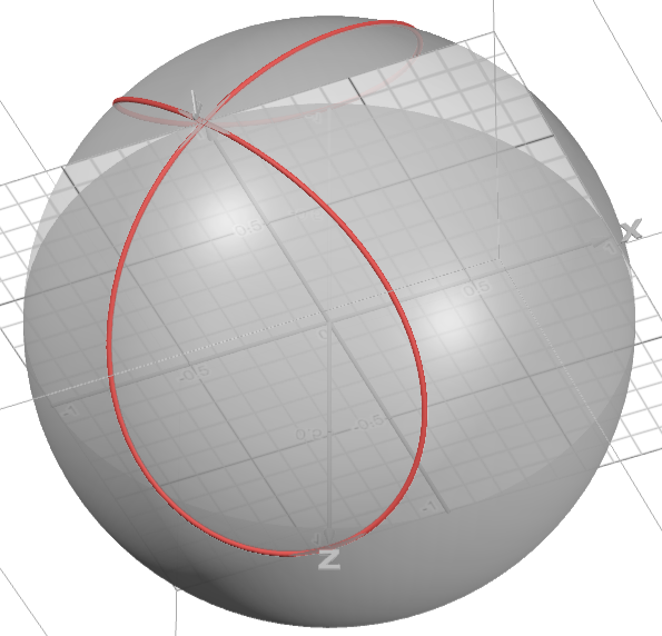
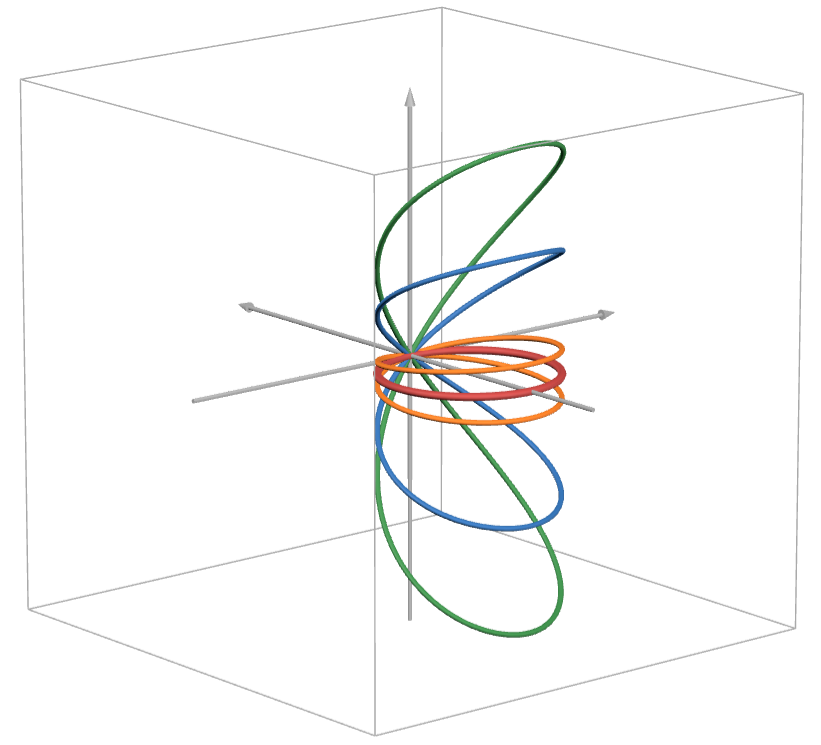
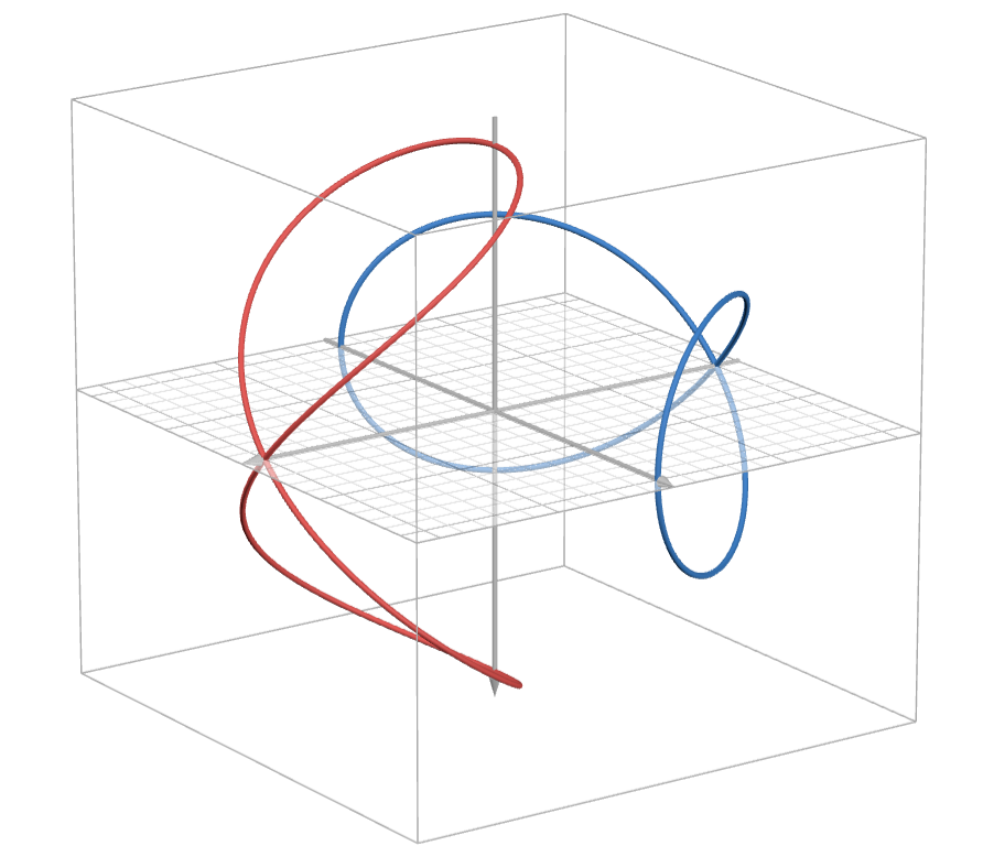
So our question in this paper is this: how do we build the real world from elementary electron and proton particle models? We speculate about that using our own simplified models, which boil down to two geometrical elements: (i) the planar or 2D ring current of the zbw electron, and (ii) the three-dimensional Lissajous trajectory on a sphere which we think might make sense when modeling the orbital of the zbw charge in a proton. Both have the advantage they involve only one frequency rather than the two frequencies (or two modes of oscillation) one sees in helical or toroidal models. Why do we prefer to stick to the idea of one frequency only, even if we readily admit helical or toroidal models are far more precise in terms of generating the experimentally measured value of the magnetic moment of electrons and protons, respectively? The answer is simple: I am just an amateur and so I like to roll with very simple things when trying to tackle something difficult. 🙂

So, go and have a look at our reflections on multi-charge Zitterbewegung models – if only because we also started writing about the history of the Zitterbewegung interpretation and a few other things. To sum it up:

  1. The paper offers a new brief history of how interpretations of the new quantum physics evolved, and why I am with Schrödinger’s Zitterbewegung hypothesis: it just explains the (possible) structure of elementary particles so well.
  2. It speculates about how positive and negative charge may combine in a neutron, and then also about how a deuteron nucleus might look like.
  3. We did not get to specific suggestions for helium-3 and helium-4 nuclei because these depend on how you think about the neutron and the deuteron nucleus. However, I do spell out why and how about I think of a neutron playing the role I think it plays in a nucleus: the glue that holds protons together (so there is no need for quark-gluon theory, I think, even if I do acknowledge the value of some triadic color scheme on top of the classical quantum numbers).
  4. Indeed, despite my aversion of the new metaphysics that crept into physics in the 1970s, I explain why the idea of some color typing (not a color charge but just an extra triadic classification of charge) might still be useful. [I secretly hope this may help me to understand why this color scheme was introduced in the 1970s, because I do not see it as anything more than mathematical factoring of matrix equations describing disequilibrium states – which may be impossible to solve.]

Have a look, even if it is only to appreciate some of the 3D images of what I think as elementary equations of motion (I copy some below). I should do more with these images. Some art, perhaps, using OpenAI’s DALL·E image generator. Who knows: perhaps AI may, one day, solve the n-body problems I write about and, thereby, come up with the ultimate interpretation of quantum mechanics?

That sounds crazy but, from one or two conversations (with real people), it looks like I am not alone with that idea. 🙂 There are good reasons why CERN turned to AI a few years ago: for the time being, they use it to detect anomalies in the jets that come out of high-energy collissions, but – who knows? – perhaps a more advanced AI Logic Theorist programme could simplify the rather messy quark-gluon hypothesis some day?

Because I am disengaging from this field (it is mentally exhausting, and one gets stuck rather quickly), I surely hope so.

Post scriptum

A researcher I was in touch with a few years ago sent me a link to the (virtual) Zitter Institute: https://www.zitter-institute.org/. It is a network and resource center for non-mainstream physicists who succesfully explored – and keep exploring, of course – local/realist interpretations of quantum mechanics by going back to Schrödinger’s original and alternative interpretation of what an electron actually is: a pointlike (but not infinitesimally small) charge orbiting around in circular motion, with:

(i) the trajectory of its motion being determined by the Planck-Einstein relation, and

(ii) an energy – given by Einstein’s mass-energy equivalence relation – which perfectly fits Wheeler’s “mass-without-mass” idea.

I started exploring Schrödinger’s hypothesis myself about ten years ago – as a full-blown alternative to the Bohr-Heisenberg interpretation of quantum mechanics (which I think of as metaphysical humbug, just like Einstein and H.A. Lorentz at the time) – and consistently blogged and published about it: here on this website, and then on viXra, Academia and, since 2020, ResearchGate. So I checked out this new site, and I see the founding members added my blog site as a resource to their project list.

[…]

I am amazingly pleased with that. I mean… My work is much simpler than that of, say, Dr. John G. Williamson (CERN/Philips Research Laboratories/Glasgow University) and Dr. Martin B. van der Mark (Philips Research Laboratories), who created the Quantum Bicycle Society (https://quicycle.com/).

So… Have a look – not at my site (I think I did not finish the work I started) but at the other resources of this new Institute: it looks like this realist and local interpretation of quantum mechanics is no longer non-mainstream… Sweet ! It makes me feel the effort I put into all of this has paid off ! 😉 Moreover, some of my early papers (2018-2020) are listed as useful papers to read. I think that is better than being published in some obscure journal. 🙂

I repeat again: my own research interest has shifted to computer science, logic and artificial intelligence now (you will see recent papers on my RG site are all about that now). It is just so much more fun and it also lines up better with my day job as a freelance IT project manager. So, yes, it is goodbye – but I am happy I can now refer all queries about my particle models and this grand synthesis between old and new quantum mechanics to the Zitter Institute.

It’s really nice: I have been in touch with about half of the founding members of this Institute over the past ten years – casually or in a more sustained way while discussing this or that 2D or 3D model of an electron, proton, or neutron), and they are all great and amazing researchers because they look for truth in science and are very much aware of this weird tendency of modern-day quantum scientists turning their ideas into best-sellers perpetuating myths and mysteries. [I am not only thinking of the endless stream of books from authors like Roger Penrose (the domain for this blog was, originally, reading Penrose rather than reading Feynman) or Graham Greene here, but also of what I now think of rather useless MIT or edX online introductions to quantum physics and quantum math.]

[…]

Looking at the website, I see the engine behind it: Dr. Oliver Consa. I was in touch with him too. He drew my attention to remarkable flip-flop articles such as William Lamb’s anti-photon article (it is an article which everyone should read, I think: unfortunately, you have to pay for it) and remarkable interviews with Freeman Dyson. Talking of the latter (I think of as “the Wolfgang Pauli of the third generation of quantum physicists” because he helped so many others to get a Nobel Prize before he got one – Dyson never got a Nobel Prize, by the way), this is one of these interviews you should watch: just four years before he would die from old age, Freeman Dyson plainly admits QED and QFT is a totally unproductive approach: a “dead end” as Dyson calls it.

So, yes, I am very pleased and happy. It makes me feel my sleepness nights and hard weekend work over the past decade on this has not been in vain ! Paraphrasing Dyson in the above-mentioned video interview, I’d say: “It is the end of the story, and that particular illumination was a very joyful time.” 🙂

Thank you, Dr. Consa. Thank you, Dr. Vassallo, Dr. Burinskii, Dr. Meulenberg, Dr. Kovacs, and – of course – Dr. Hestenes – who single-handedly revived the Zitterbewegung interpretation of quantum mechanics in the 1990s. I am sure I forgot to mention some people. Sorry for that. I will wrap up my post here by saying a few more words about David Hestenes.

I really admire him deeply. Moving away from the topic of high-brow quantum theory, I think his efforts to reform K-12 education in math and physics is even more remarkable than the new space-time algebra (STA) he invented. I am 55 years old and so I know all about the small and pleasant burden to help kids with math and statistics in secondary school and at university: the way teachers now have to convey math and physics to kids now is plain dreadful. I hope it will get better. It has to. If the US and the EU want to keep leading in research, then STEM education (Science, Technology, Engineering, and Mathematics) needs a thorough reform. :-/

Another tainted Nobel Prize…

Last year’s (2022) Nobel Prize in Physics went to Alain Aspect, John Clauser, and Anton Zeilinger for “for experiments with entangled photons, establishing the violation of Bell inequalities and pioneering quantum information science.”

I did not think much of that award last year. Proving that Bell’s No-Go Theorem cannot be right? Great. Finally! I think many scientists – including Bell himself – already knew this theorem was a typical GIGO argument: garbage in, garbage out. As the young Louis de Broglie famously wrote in the introduction of his thesis: hypotheses are worth only as much as the consequences that can be deduced from it, and the consequences of Bell’s Theorem did not make much sense. As I wrote in my post on it, Bell himself did not think much of his own theorem until, of course, he got nominated for a Nobel Prize: it is a bit hard to say you got nominated for a Nobel Prize for a theory you do not believe in yourself, isn’t it? In any case, Bell’s Theorem has now been experimentally disproved. That is – without any doubt – a rather good thing. 🙂 To save the face of the Nobel committee here (why award something that disproves something else that you would have given an award a few decades ago?): Bell would have gotten a Nobel Prize, but he died from brain hemorrhage before, and Nobel Prizes reward the living only.

As for entanglement, I repeat what I wrote many times already: the concept of entanglement – for which these scientists got a Nobel Prize last year – is just a fancy word for the simultaneous conservation of energy, linear and angular momentum (and – if we are talking matter-particles – charge). There is ‘no spooky action at a distance’, as Einstein would derogatorily describe it when the idea was first mentioned to him. So, I do not see why a Nobel Prize should be awarded for rephrasing a rather logical outcome of photon experiments in metamathematical terms.

Finally, the Nobel Prize committee writes that this has made a significant contribution to quantum information science. I wrote a paper on the quantum computing hype, in which I basically ask this question: qubits may or may not be better devices than MOSFETs to store data – they are not, and they will probably never be – but that is not the point. How does quantum information change the two-, three- or n-valued or other rule-based logic that is inherent to the processing of information? I wish the Nobel Prize committee could be somewhat more explicit on that because, when everything is said and done, one of the objectives of the Prize is to educate the general public about the advances of science, isn’t it? :-/

However, all this ranting of mine is, of course, unimportant. We know that it took the distinguished Royal Swedish Science Academy more than 15 years to even recognize the genius of an Einstein, so it was already clear then that their selection criteria were not necessarily rational. [Einstein finally got a well-deserved Nobel Prize, not for relativity theory (strangely enough: if there is one thing on which all physicist are agreed, it is that relativity theory is the bedrock of all of physics, isn’t it?), but for a much less-noted paper on the photoelectric effect – in 1922: 17 years after his annus mirabilis papers had made a killing not only in academic circles but in the headlines of major newspapers as well, and 10 years after a lot of fellow scientists had nominated him for it (1910).]

Again, Mahatma Gandhi never got a Nobel Price for Peace (so Einstein should consider himself lucky to get some Nobel Prize, right?), while Ursula von der Leyen might be getting one for supporting the war with Russia, so I must remind myself of the fact that we do live in a funny world and, perhaps, we should not be trying to make sense of these rather weird historical things. 🙂

Let me turn to the main reason why I am writing this indignant post. It is this: I am utterly shocked by what Dr. John Clauser has done with his newly gained scientific prestige: he joined the CO2 coalition! For those who have never heard of it, it is a coalition of climate change deniers. A bunch of people who:

(1) vehemently deny the one and only consensus amongst all climate scientists, and that is the average temperature on Earth has risen with about two degrees Celsius since the Industrial Revolution, and

(2) say that, if climate change would be real (God forbid!), then we can reverse the trend by easy geo-engineering. We just need to use directed energy or whatever to create more white clouds. If that doesn’t work, then… Well… CO2 makes trees and plants grow, so it will all sort itself out by itself.

[…]

Yes. That is, basically, what Dr. Clauser and all the other scientific advisors of this lobby group – none of which have any credentials in the field they are criticizing (climate science) – are saying, and they say it loud and clearly. That is weird enough, already. What is even weirder, is that – to my surprise – a lot of people are actually buying such nonsense.

Frankly, I have not felt angry for a while, but this thing triggered an outburst of mine on YouTube, in which I state clearly what I think of Dr. Clauser and other eminent scientists who abuse their saint-like Nobel Prize status in society to deceive the general public. Watch my video rant, and think about it for yourself. Now, I am not interested in heated discussions on it: I know the basic facts. If you don’t, I listed them here. Look at the basic graphs and measurements before you would want to argue with me on this, please! To be clear on this: I will not entertain violent or emotional reactions to this post or my video. Moreover, I will delete them here on WordPress and also on my YouTube channel. Yes. For the first time in 10 years or so, I will exercise my right as a moderator of my channels, which is something I have never done before. 🙂

[…]

I will now calm down and write something about the mainstream interpretation of quantum physics again. 🙂 In fact, this morning I woke up with a joke in my head. You will probably think the joke is not very good, but then I am not a comedian and so it is what it is and you can judge for yourself. The idea is that you’d learn something from it. Perhaps. 🙂 So, here we go.

Imagine shooting practice somewhere. A soldier fires at some target with a fine gun, and then everyone looks at the spread of the hits around the bullseye. The quantum physicist says: “See: this is the Uncertainty Principle at work! What is the linear momentum of these bullets, and what is the distance to the target? Let us calculate the standard error.” The soldier looks astonished and says: “No. This gun is no good. One of the engineers should check it.” Then the drill sergeant says this: “The gun is fine. From this distance, all bullets should have hit the bullseye. You are a miserable shooter and you should really practice a lot more.” He then turns to the academic and says: “How did you get in here? I do not understand a word of what you just said and, if I do, it is of no use whatsoever. Please bugger off asap!”

This is a stupid joke, perhaps, but there is a fine philosophical point to it: uncertainty is not inherent to Nature, and it also serves no purpose whatsoever in the science of engineering or in science in general. All in Nature is deterministic. Statistically deterministic, but deterministic nevertheless. We do not know the initial conditions of the system, perhaps, and that translates into seemingly random behavior, but if there is a pattern in that behavior (a diffraction pattern, in the case of electron or photon diffraction), then the conclusion should be that there is no such thing as metaphysical ‘uncertainty’. In fact, if you abandon that principle, then there is no point in trying to discover the laws of the Universe, is there? Because if Nature is uncertain, then there are no laws, right? 🙂

To underscore this point, I will, once again, remind you of what Heisenberg originally wrote about uncertainty. He wrote in German and distinguished three very different ideas of uncertainty:

(1) The precision of our measurements may be limited: Heisenberg originally referred to this as an Ungenauigkeit.

(2) Our measurement might disturb the position and, as such, cause the information to get lost and, as a result, introduce an uncertainty in our knowledge, but not in reality. Heisenberg originally referred to such uncertainty as an Unbestimmtheit.

(3) One may also think the uncertainty is inherent to Nature: that is what Heisenberg referred to as Ungewissheit. There is nothing in Nature – and also nothing in Heisenberg’s writings, really – that warrants the elevation of this Ungewissheit to a dogma in modern physics. Why? Because it is the equivalent of a religious conviction, like God exists or He doesn’t (both are theses we cannot prove: Ryle labeled such hypotheses as ‘category mistakes’).

Indeed, when one reads the proceedings of the Solvay Conferences of the late 1920s, 1930s and immediately after WW II (see my summary of it in https://www.researchgate.net/publication/341177799_A_brief_history_of_quantum-mechanical_ideas), then it is pretty clear that none of the first-generation quantum physicists believed in such dogma and – if they did – that they also thought what I am writing here: that it should not be part of science but part of one’s personal religious beliefs.

So, once again, I repeat that this concept of entanglement – for which John Clauser got a Nobel Prize last year – is in the same category: it is just a fancy word for the simultaneous conservation of energy, linear and angular momentum, and charge. There is ‘no spooky action at a distance’, as Einstein would derogatorily describe it when the idea was first mentioned to him.

Let me end by noting the dishonor of Nobel Prize winner John Clauser once again. Climate change is real: we are right in the middle of it, and it is going to get a lot worse before it gets any better – if it is ever going to get better (which, in my opinion, is a rather big ‘if‘…). So, no matter how many Nobel Prize winners deny it, they cannot change the fact that average temperature on Earth has risen by about 2 degrees Celsius since 1850 already. The question is not: is climate change happening? No. The question now is: how do we adapt to it – and that is an urgent question – and, then, the question is: can we, perhaps, slow down the trend, and how? In short, if these scientists from physics or the medical field or whatever other field they excel in are true and honest scientists, then they would do a great favor to mankind not by advocating geo-engineering schemes to reverse a trend they actually deny is there, but by helping to devise and promote practical measures to allow communities that are affected by natural disaster to better recover from them.

So, I’ll conclude this rant by repeating what I think of all of this. Loud and clear: John Clauser and the other scientific advisors of the CO2 coalition are a disgrace to what goes under the name of ‘science’, and this umpteenth ‘incident’ in the history of science or logical thinking makes me think that it is about time that the Royal Swedish Academy of Sciences does some serious soul-searching when, amongst the many nominations, it selects its candidates for a prestigious award like this. Alfred Nobel – one of those geniuses who regretted his great contribution to science and technology was (also) (ab)used to increase the horrors of war – must have turned too many times in his grave now… :-/

The End of Physics

I wrote a post with this title already, but this time I mean it in a rather personal way: my last paper – with the same title – on ResearchGate sums up rather well whatever I achieved, and also whatever I did not explore any further because time and energy are lacking: I must pay more attention to my day job nowadays. 🙂

I am happy with the RG score all of my writing generated, the rare but heartfelt compliments I got from researchers with far more credentials than myself (such as, for example, Dr. Emmanouil Markoulakis of Nikolaos, which led me to put a paper on RG with a classical explanation of the Lamb shift), various friendly but not necessarily always agreeing commentators (one of them commenting here on this post: a good man!), and, yes, the interaction on my YouTube channel. But so… Well… That is it, then! 🙂

As a farewell, I will just quote from the mentioned paper – The End of Physics (only as a science, of course) – hereunder, and I hope that will help you to do what all great scientists would want you to do, and that is to think things through for yourself. 🙂

Brussels, 22 July 2023

Bohr, Heisenberg, and other famous quantum physicists – think of Richard Feynman, John Stewart Bell, Murray Gell-Mann, and quite a few other Nobel Prize winning theorists[1] – have led us astray. They swapped a rational world view – based on classical electromagnetic theory and statistical determinism – for a mystery world in which anything is possible, but nothing is real.

They invented ‘spooky action at a distance’ (as Einstein derogatorily referred to it), for example. So, what actually explains that long-distance interaction, then? It is quite simple. There is no interaction, and so there is nothing spooky or imaginary or unreal about it: if by measuring the spin state of one photon, we also know the spin state of its twin far away, then it is – quite simply – because physical quantities such as energy and momentum (linear or angular) will be conserved if no other interference is there after the two matter- or light-particles were separated.

Plain conservation laws explain many other things that are being described as ‘plain mysteries’ in quantum physics. The truth is this: there are no miracles or mysteries: everything has a physical cause and can be explained.[2] For example, there is also nothing mysterious about the interference pattern and the trajectory of an electron going through a slit, or one of two nearby slits. An electron is pointlike, but it is not infinitesimally small: it has an internal structure which explains its wave-like properties. Likewise, Mach-Zehnder one-photon interference can easily be explained when thinking of its polarization structure: a circularly polarized photon can be split in two linearly polarized electromagnetic waves, which are photons in their own right. Everything that you have been reading about mainstream quantum physics is, perhaps, not wrong, but it is highly misleading because it is all couched in guru language and mathematical gibberish.

Why is that mainstream physicists keep covering up? I am not sure: it is a strange mix of historical accident and, most probably, the human desire to be original or special, or the need to mobilize money for so-called fundamental research. I also suspect there is a rather deceitful intention to hide truths about what nuclear science should be all about, and that is to understand the enormous energies packed into elementary particles.[3]

The worst of all is that none of the explanations in mainstream quantum physics actually works: mainstream theory does not have a sound theory of signal propagation, for example (click the link to my paper on that or – better, perhaps – this link to our paper on signal propagation), and Schrödinger’s hydrogen model is a model of a hypothetical atom modelling orbitals of equally hypothetical zero-spin electron pairs. Zero-spin electrons do not exist, and real-life hydrogen only has one proton at its center, and one electron orbiting around it. Schrödinger’s equation is relativistically correct – even if all mainstream physicists think it is not – but the equation includes two mistakes that cancel each other out: it confuses the effective mass of an electron in motion with its total mass[4], and the 1/2 factor which is introduced by the m = 2meff substitution also takes care of the doubling of the potential that is needed to make the electron orbitals come out alright.

The worst thing of all is that mainstream quantum physicists never accurately modeled what they should have modeled: the hydrogen atom as a system of a real proton and a real electron (no hypothetical infinitesimally and structureless spin-zero particles). If they had done that, they would also be able to explain why hydrogen atoms come in molecular H2 pairs, and they would have a better theory of why two protons need a neutron to hold together in a helium nucleus. Moreover, they would have been able to explain what a neutron actually is.[5]


[1] James Stewart Bell was nominated for a Nobel Prize, but died from a brain hemorrhage before he could accept the prize for his theorem.

[2] The world of physics – at the micro-scale – is already fascinating enough: why should we invent mysteries?

[3] We do not think these energies can be exploited any time soon. Even nuclear energy is just binding energy between protons and neutrons: a nuclear bomb does not release the energy that is packed into protons. These elementary particles survive the blast: they are the true ‘atoms’ of this world (in the Greek sense of ‘a-tom’, which means indivisible).

[4] Mass is a measure of the inertia to a change in the state of motion of an oscillating charge. We showed how this works by explaining Einstein’s mass-energy equivalence relation and clearly distinguishing the kinetic and potential energy of an electron. Feynman first models an electron in motion correctly, with an equally correct interpretation of the effective mass of an electron in motion, but then substitutes this effective mass by half the electron mass (meff = m/2) in an erroneous reasoning process based on the non-relativistic kinetic energy concept. The latter reasoning also leads to the widespread misconception that Schrödinger’s equation would not be relativistically correct (see the Annexes to my paper on the matter-wave). For the trick it has to do, Schrödinger’s wave equation is correct – and then I mean also relativistically correct. 🙂

[5] A neutron is unstable outside of its nucleus. We, therefore, think it acts as the glue between protons, and it must be a composite particle.

On the quantum computing hype

1. The Wikipedia article on quantum computing describes a quantum computer as “a computer that exploits quantum -mechanical phenomena.” The rest of the article then tries to explain what these quantum-mechanical phenomena actually are.

Unfortunately, the article limits itself to the mainstream interpretation of these and, therefore, suffers from what I perceive to be logical and philosophical errors. Indeed, in the realistic interpretation of quantum mechanics that I have been developing, system wavefunctions are only useful to model our own uncertainty about the system. I subscribe to Hendrik Antoon Lorentz’s judgment at the last Solvay Conference under his leadership: there is no need whatsoever to elevate indeterminism to a philosophical principle. Not in science in general, and not in quantum mechanics in particular. I, therefore, think quantum mechanics cannot offer a substantially new computing paradigm.

Of course, one may argue that, for specific problems, some kind of three- or more-valued logic – rather than the binary or Boolean true/false dichotomy on which most logic circuits are based – may come in handy. However, such logic has already been worked out, and can be accessed using appropriate programming languages. Python and the powerful mathematical tools that come with it (Pandas, NumPy and SciPy) work great with ternary logic using a {true, false, unknown} or a {-1, 0, +1} set of logical values rather than the standard {0, 1} Boolean set. The Wikipedia article on three-valued logic is worth a read and, despite the rather arcane nature of the topic, much better written than the mentioned article: have a look at how operators are used on these three-valued sets in meaningful algebras or logical models, such as that of Kleene, Priest or Lukasiewicz.

2. One may, of course, argue that, even when there is probably no such thing as a new logical quantum computing model or logic, quantum technology may offer distinct advantages when it comes to storage of data about this or that state or, one day, lead to devices with faster clock and/or bus speeds. That appears to be a pipedream too:

  • To keep, say, an electron in this or that spin state, one must create and steady an electromagnetic field – usually one does so in a superconducting environment, which makes actual mechanical devices used for quantum computing (qubits) look like the modern-day equivalent of Babbage’s analytical machine. In my not-so-humble view, such devices will never ever achieve the sheer material performance offered by current nanometer-scale MOSFETs.  

  • As for bus or transmission speeds, quantum theory does not come with a new theory of charge propagation and, most importantly, is fundamentally flawed in its analysis of how signals actually propagate in, say, a lattice structure. I refer to one of my papers here (on electron propagation in a lattice), in which I deconstruct Feynman’s analysis of the concept of the free and effective mass of an electron. Hence, for long-distance transmission of signals, optical fiber cannot be beaten. For short-distance transmission of signals (say, within an electrical circuit, I refer to the above-mentioned nano-technology which continues to revolutionize the chip industry.

Brussels, 4 July 2023

Epilogue: an Easter podcast

I have been thinking on my explanation of dark matter/energy, and I think it is sound. It solves the last asymmetry in my models, and explains all. So, after a hiatus of two years, I bothered to make a podcast on my YouTube channel once again. It talks about everything. Literally everything !

It makes me feel my quest for understanding of matter and energy – in terms of classical concepts and measurements (as depicted below) – has ended. Perhaps I will write more but that would only be to promote the material, which should promote itself if it is any good (which I think it is).

I should, by way of conclusion, say a few final words about Feynman’s 1963 Lectures now. When everything is said and done, it is my reading of them which had triggered this blog about ten years ago. I would now recommend Volume I and II (classical physics and electromagnetic theory) – if only because it gives you all the math you need to understand all of physics – but not Volume III (the lectures on quantum mechanics). They are outdated, and I do find Feynman guilty of promoting rather than explaining the hocus-pocus around all of the so-called mysteries in this special branch of physics.

Quantum mechanics is special, but I do conclude now that it can all be explained in terms of classical concepts and quantities. So, Gell-Mann’s criticism of Richard Feynman is, perhaps, correct: Mr. Feynman did, perhaps, make too many jokes – and it gets annoying because he must have known some of what he suggests does not make sense – even if I would not go as far as Gell-Mann, who says “Feynman was only concerned about himself, his ego, and his own image !” :-/

So, I would recommend my own alternative series of ‘lectures’. Not only are they easier to read, but they also embody a different spirit of writing. Science is not about you, it is about thinking for oneself and deciding on what is truthful and useful, and what is not. So, to conclude, I will end by quoting Ludwig Boltzmann once more:

“Bring forward what is true.

Write it so that it is clear.

Defend it to your last breath.”

Ludwig Boltzmann (1844 – 1906)

Post scriptum: As for the ‘hocus-pocus’ in Feynman’s Lectures, we should, perhaps, point once again to some of our early papers on the flaws in his arguments. We effectively put our finger on the arbitrary wavefunction convention, or the (false) boson-fermion dichotomy, or the ‘time machine’ argument that is inherent to his explanation of the Hamiltonian, and so on. We published these things on Academia.edu before (also) putting our (later) papers ResearchGate, so please check there for the full series. 🙂

Post scriptum (23 April 2023): Also check out this video, which was triggered by someone who thought my models amount to something like a modern aether theory, which it is definitely not the case: https://www.youtube.com/watch?v=X38u2-nXoto. 🙂 I really think it is my last reflection on these topics. I need to focus on my day job, sports, family, etcetera again ! 🙂

Onwards !

It has been ages since I last wrote something here. Regular work took over. I did do an effort, though, to synchronize and reorganize some stuff. And I am no longer shy about it. My stats on ResearchGate and academia.edu show that I am no longer a ‘crackpot theorist’. This is what I wrote about it on my LinkedIn account:

QUOTE

With good work-life balance now, I picked up one of my hobbies again: research into quantum theories. As for now, I only did a much-needed synchronization of papers on academia.edu and ResearchGate. When logging on the former network (which I had not done for quite a while), I found many friendly messages on it. One of them was from a researcher on enzymes: “I have been studying about these particles for around four years. All of the basics. But wat are they exactly? This though inspired me… Thank u so much!” I smiled and relaxed when I read that, telling myself that all those sleepless nights I spent on this were not the waste of time and energy that most of my friends thought it would be. 🙂

Another one was even more inspiring. It was written by another ‘independent’ researcher. Nelda Evans. No further detail in her profile. From the stats, I could see that she had downloaded an older manuscript of mine (https://lnkd.in/ecRKJwxQ). This is what she wrote about it to me: “I spoke to Richard Feynman in person at the Hughes Research Lab in Malibu California in 1967 where the first pulsed laser was invented when some of the students from the UCLA Physics Dept. went to hear him. Afterward I went to talk to him and said “Dr. Feynman, I’ve learned that some unknown scientists were dissatisfied with probability as a final description of Quantum Mechanics, namely Planck, Einstein, Schrodinger, de Broglie, Bohm,…” When I finished my list he immediately said “And Feynman”. We talked about it a little, and he told me “I like what you pick on.”
My guess is that he might have told you something similar.”

That message touched me deeply, because I do feel – from reading his rather famous Lectures on Physics somewhat ‘between the lines’ – that Richard Feynman effectively knew all but that he, somehow, was not allowed to clearly say what it was all about. I wrote a few things about that rather strange historical bias in the interpretation of ‘uncertainty’ and other ‘metaphysical’ concepts that infiltrated the science of quantum mechanics in my last paper: https://lnkd.in/ewZBcfke.

So… Well… I am not a crackpot scientist anymore ! 🙂 The bottom-line is to always follow your instinct when trying to think clearly about some problem or some issue. We should do what Ludwig Boltzmann (1844-1906) told us to do: “Bring forward what is true. Write it so that it is clear. Defend it to your last breath.”

[…] Next ‘thing to do’, is to chat with ChatGPT about my rather straightforward theories. I want to see how ‘intelligent’ it is. I wonder where it will hit its limit in terms of ‘abstract thinking.’ The models I worked on combine advanced geometrical thinking (building ‘realistic’ particle models requires imagining ‘rotations within rotations’, among other things) and formal math (e.g. quaternion algebra). ChatGPT is excellent in both, I was told, but can it combine the two intelligently? 🙂

UNQUOTE

On we go. When the going gets tough, the tough get going. 🙂 For those who want an easy ‘introduction’ to the work (at a K-12 level of understanding of mathematics), I wrote the first pages of what could become a very new K-12 level textbook on physics. Let us see. I do want to see some interest from a publisher first. 🙂

Deep electron orbitals and the essence of quantum physics

After a long break (more than six months), I have started to engage again in a few conversations. I also looked at the 29 papers on my ResearchGate page, and I realize some of them would need to be re-written or re-packaged so as to ensure a good flow. Also, some of the approaches were more productive than others (some did not lead anywhere at all, actually), and I would need to point those out. I have been thinking about how to approach this, and I think I am going to produce an annotated version of these papers, with comments and corrections as mark-ups. Re-writing or re-structuring all of them would require to much work.

The mark-up of those papers is probably going to be based on some ‘quick-fire’ remarks (a succession of thoughts triggered by one and the same question) which come out of the conversation below, so I thank these thinkers for having kept me in the loop of a discussion I had followed but not reacted to. It is an interesting one – on the question of ‘deep electron orbitals’ (read: the orbitals of negative charge inside of a nucleus exist and, if so, how one can model them. If one could solve that question, one would have a theoretical basis for what is referred to as low-energy nuclear reactions. That was known formerly as cold fusion, but that got a bit of a bad name because of a number of crooks spoiling the field, unfortunately.

PS: I leave the family names of my correspondents in the exchange below out so they cannot be bothered. One of them, Jerry, is a former American researcher at SLAC. Andrew – the key researcher on DEPs – is a Canadian astrophysicist, and the third one – Jean-Luc – is a rather prominent French scientist in LENR.]

From: Jean Louis Van Belle
Sent: 18 November 2021 22:51
Subject: Staying engaged (5)

Oh – and needless to say, Dirac’s basic equation can, of course, be expanded using the binomial expansion – just like the relativistic energy-momentum relation, and then one can ‘cut off’ the third-, fourth-, etc-order terms and keep the first and second-order terms only. Perhaps it is equations like that kept you puzzled (I should check your original emails). In any case, this way of going about energy equations for elementary particles is a bit the same as those used in perturbation equations in which – as Dirac complained – one randomly selects terms that seem to make sense and discard others because they do not seem to make sense. Of course, Dirac criticized perturbation theory much more severely than this – and rightly so. 😊 😊 JL

From: Jean Louis Van Belle
Sent: 18 November 2021 22:10
Subject: Staying engaged (4)

Also – I remember you had some questions on an energy equation – not sure which one – but so I found Dirac’s basic equation (based on which he derives the ‘Dirac’ wave equation) is essentially useless because it incorporates linear momentum only. As such, it repeats de Broglie’s mistake, and that is to interpret the ‘de Broglie’ wavelength as something linear. It is not: frequencies, wavelengths are orbital frequencies and orbital circumferences. So anything you would want to do with energy equations that are based on that, lead nowhere – in my not-so-humble opinion, of course. To illustrate the point, compare the relativistic energy-momentum relation and Dirac’s basic equation in his Nobel Prize lecture (I hope the subscripts/superscripts get through your email system so they display correctly):

m02c4 = E2 – p2c2 (see, for example, Feynman-I-16, formula 16-3)

Divide the above by c2 and re-arrange and you get Dirac’s equation: W2/c2 – pr2 – m2/c2 = 0 (see his 1933 Nobel Prize Lecture)

So that cannot lead anywhere. It’s why I totally discard Dirac’s wave equation (it has never yielded any practical explanation of a real-life phenomenon anyway, if I am not mistaken).

Cheers – JL

From: Jean Louis Van Belle
Sent: 18 November 2021 21:49
Subject: Staying engaged (3)

Just on ‘retarded sources’ and ‘retarded fields’ – I have actually tried to think of the ‘force mechanism’ inside of an electron or a proton (what keeps the pointlike charge in this geometric orbit around a center of mass?). I thought long and hard about some kind of model in which we have the charge radiate out a sub-Planck field, and that its ‘retarded effects’ might arrive ‘just in time’ to the other side of the orbital (or whatever other point on the orbital) so as to produce the desired ‘course correction’ might explain it. I discarded it completely: I am now just happy that we have ‘reduced’ the mystery to this ‘Planck-scale quantum-mechanical oscillation’ (in 2D or 3D orbitals) without the need for an ‘aether’, or quantized spacetime, or ‘virtual particles’ actually ‘holding the thing together’.

Also, a description in terms of four-vectors (scalar and vector potential) does not immediately call for ‘retarded time’ variables and all that, so that is another reason why I think one should somehow make the jump from E-B fields to scalar and vector potential, even if the math is hard to visualize. If we want to ‘visualize’ things, Feynman’s discussion of the ‘energy’ and ‘momentum’ flow in https://www.feynmanlectures.caltech.edu/II_27.html might make sense, because I think analyses in terms of Poynting vectors are relativistically current, aren’t they? It is just an intuitive idea…

Cheers – JL

From: Jean Louis Van Belle
Sent: 18 November 2021 21:28
Subject: Staying engaged (2)

But so – in the shorter run – say, the next three-six months, I want to sort out those papers on ResearchGate. The one on the de Broglie’s matter-wave (interpreting the de Broglie wavelength as the circumference of a loop rather than as a linear wavelength) is the one that gets most downloads, and rightly so. The rest is a bit of a mess – mixing all kinds of things I tried, some of which worked, but other things did not. So I want to ‘clean’ that up… 😊 JL

From: Jean Louis Van Belle
Sent: 18 November 2021 21:21
Subject: Staying engaged…

Please do include me in the exchanges, Andrew – even if I do not react, I do read them because I do need some temptation and distraction. As mentioned, I wanted to focus on building a credible n = p + e model (for free neutrons but probably more focused on a Schrodinger-like D = p + e + p Platzwechsel model, because the deuteron nucleus is stable). But so I will not do that the way I studied the zbw model of the electron and proton (I believe that is sound now) – so that’s with not putting in enough sleep. I want to do it slowly now. I find a lot of satisfaction in the fact that I think there is no need for complicated quantum field theories (fields are quantized, but in a rather obvious way: field oscillations – just like matter-particles – pack Planck’s quantum of (physical) action which – depending on whether you freeze time or positions as a variable, expresses itself as a discrete amount of energy or, alternatively, as a discrete amount of momentum), nor is there any need for this ‘ontologization’ of virtual field interactions (sub-Planck scale) – the quark-gluon nonsense.

Also, it makes sense to distinguish between an electromagnetic and a ‘strong’ or ‘nuclear’ force: the electron and proton have different form factors (2D versus 3D oscillations, but that is a bit of a non-relativistic shorthand for what might be the case) but, in addition, there is clearly a much stronger force at play within the proton – whose strength is the same kind of ‘scale’ as the force that gives the muon-electron its rather enormous mass. So that is my ‘belief’ and the ‘heuristic’ models I build (a bit of ‘numerology’ according to Dr Pohl’s rather off-hand remarks) support it sufficiently for me to make me feel at peace about all these ‘Big Questions’.

I am also happy I figured out these inconsistencies around 720-degree symmetries (just the result of a non-rigorous application of Occam’s Razor: if you use all possible ‘signs’ in the wavefunction, then the wavefunction may represent matter as well as anti-matter particles, and these 720-degree weirdness dissolves). Finally, the kind of ‘renewed’ S-matrix programme for analyzing unstable particles (adding a transient factor to wavefunctions) makes sense to me, but even the easiest set of equations look impossible to solve – so I may want to dig into the math of that if I feel like having endless amounts of time and energy (which I do not – but, after this cancer surgery, I know I will only die on some ‘moral’ or ‘mental’ battlefield twenty or thirty years from now – so I am optimistic).

So, in short, the DEP question does intrigue me – and you should keep me posted, but I will only look at it to see if it can help me on that deuteron model. 😊 That is the only ‘deep electron orbital’ I actually believe in. Sorry for the latter note.

Cheers – JL   

From: Andrew
Sent: 16 November 2021 19:05
To: Jean-Luc; Jerry; Jean Louis
Subject: Re: retarded potential?

Dear Jean-Louis,

Congratulations on your new position. I understand your present limitations, despite your incredible ability to be productive. They must be even worse than those imposed by my young kids and my age. Do you wish for us to not include you in our exchanges on our topic? Even with no expectation of your contributing at this point, such emails might be an unwanted temptation and distraction.

Dear Jean-Luc,

Thank you for the Wiki-Links. They are useful. I agree that the 4-vector potential should be considered. Since I am now considering the nuclear potentials as well as the deep orbits, it makes sense to consider the nuclear vector potentials to have an origin in the relativistic Coulomb potentials. I am facing this in my attempts to calculate the deep orbits from contributions to the potential energies that have a vector component, which non-rel Coulomb potentials do not have.

For examples: do we include the losses in Vcb (e.g., from the binding energy BE) when we make the relativistic correction to the potential; or, how do we relativistically treat pseudo potentials such as that of centrifugal force? We know that for equilibrium, the average forces must cancel. However, I’m not sure that it is possible to write out a proper expression for “A” to fit such cases.

Best regards to all,

Andrew

_ _ _

On Fri, Nov 12, 2021 at 1:42 PM Jean-Luc wrote:

Dear all,

I totally agree with the sentence of Jean-Louis, which I put in bold in his message, about vector potential and scalar potential, combined into a 4-vector
potential A
, for representing EM field in covariant formulation. So EM representation by 4-vector A has been very developed, as wished by JL,
in the framework of QED.

We can note the simplicity of Lorentz gauge written by using A.
   https://en.wikipedia.org/wiki/Lorenz_gauge_condition

We can see the reality of vector potential
in the Aharonov-Bohm effect:
    https://en.wikipedia.org/wiki/Aharonov-Bohm_effect.
In fact, we can see that vector potential contains more information than E,B fields.
Best regards

   Jean-Luc
Le 12/11/2021 à 05:43, Jean Louis Van Belle a écrit :

Hi All – I’ve been absent in the discussion, and will remain absent for a while. I’ve been juggling a lot of work – my regular job at the Ministry of Interior (I got an internal promotion/transfer, and am working now on police and security sector reform) plus consultancies on upcoming projects in Nepal. In addition, I am still recovering from my surgery – I got a bad flue (not C19, fortunately) and it set back my auto-immune system, I feel. I have a bit of a holiday break now (combining the public holidays of 11 and 15 November in Belgium with some days off to bridge so I have a rather nice super-long weekend – three in one, so to speak).

As for this thread, I feel like it is not ‘phrasing’ the discussion in the right ‘language’. Thinking of E-fields and retarded potential is thinking in terms of 3D potential, separating out space and time variables without using the ‘power’ of four-vectors (four-vector potential, and four-vector space-time). It is important to remind ourselves that we are measuring fields in continuous space and time (but, again, this is relativistic space-time – so us visualizing a 3D potential at some point in space is what it is: we visualize something because our mind needs that – wants that). The fields are discrete, however: a field oscillation packs one unit of Planck – always – and Planck’s quantum of action combines energy and momentum: we should not think of energy and momentum as truly ‘separate’ (discrete) variables, just like we should not think of space and time as truly ‘separate’ (continuous) variables.

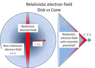
I do not quite know what I want to say here – or how I should further work it out. I am going to re-read my papers. I think I should further develop the last one (https://www.researchgate.net/publication/351097421_The_concepts_of_charge_elementary_ring_currents_potential_potential_energy_and_field_oscillations), in which I write that the vector potential is more real than the electric field and the scalar potential should be further developed, and probably it is the combined scalar and vector potential that are the ’real’ things. Not the electric and magnetic field. Hence, illustrations like below – in terms of discs and cones in space – do probably not go all that far in terms of ‘understanding’ what it is going on… It’s just an intuition…

Cheers – JL

From: Andrew
Sent: 23 September 2021 17:17
To: Jean-Luc; Jerry; Jean Louis
Subject: retarded potential?

Dear Jean-Luc,

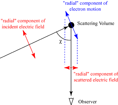
Becasue of the claim that gluons are tubal, I have been looking at the disk-shaped E-field lines of the highly-relativistic electron and comparing it to the retarded potential, which, based on timing, would seem to give a cone rather than a disk (see figure). This makes a difference when we consider a deep-orbiting electron. It even impacts selection of the model for impact of an electron when considering diffraction and interference.

Even if the field appears to be spreading out as a cone, the direction of the field lines are that of a disk from the retarded source. However, how does it interact with the radial field of a stationary charge?

Do you have any thoughts on the matter.

Best regards,

Andrew

_ _ _

On Thu, Sep 23, 2021 at 5:05 AM Jean-Luc wrote:

Dear Andrew, Thank you for the references. Best regards, Jean-Luc

Le 18/09/2021 à 17:32, Andrew a écrit :
> This might have useful thoughts concerning the question of radiation
> decay to/from EDOs.
>
> Quantum Optics Electrons see the quantum nature of light
> Ian S. Osborne
> We know that light is both a wave and a particle, and this duality
> arises from the classical and quantum nature of electromagnetic
> excitations. Dahan et al. observed that all experiments to date in
> which light interacts with free electrons have been described with
> light considered as a wave (see the Perspective by Carbone). The
> authors present experimental evidence revealing the quantum nature of
> the interaction between photons and free electrons. They combine an
> ultrafast transmission electron microscope with a silicon-photonic
> nanostructure that confines and strengthens the interaction between
> the light and the electrons. The “quantum” statistics of the photons
> are imprints onto the propagating electrons and are seen directly in
> their energy spectrum.
> Science, abj7128, this issue p. 1324; see also abl6366, p. 1309

The metaphysics of physics

I realized that my last posts were just some crude and rude soundbites, so I thought it would be good to briefly summarize them into something more coherent. Please let me know what you think of it.

The Uncertainty Principle: epistemology versus physics

Anyone who has read anything about quantum physics will know that its concepts and principles are very non-intuitive. Several interpretations have therefore emerged. The mainstream interpretation of quantum mechanics is referred to as the Copenhagen interpretation. It mainly distinguishes itself from more frivolous interpretations (such as the many-worlds and the pilot-wave interpretations) because it is… Well… Less frivolous. Unfortunately, the Copenhagen interpretation itself seems to be subject to interpretation.

One such interpretation may be referred to as radical skepticism – or radical empiricism[1]: we can only say something meaningful about Schrödinger’s cat if we open the box and observe its state. According to this rather particular viewpoint, we cannot be sure of its reality if we don’t make the observation. All we can do is describe its reality by a superposition of the two possible states: dead or alive. That’s Hilbert’s logic[2]: the two states (dead or alive) are mutually exclusive but we add them anyway. If a tree falls in the wood and no one hears it, then it is both standing and not standing. Richard Feynman – who may well be the most eminent representative of mainstream physics – thinks this epistemological position is nonsensical, and I fully agree with him:

“A real tree falling in a real forest makes a sound, of course, even if nobody is there. Even if no one is present to hear it, there are other traces left. The sound will shake some leaves, and if we were careful enough we might find somewhere that some thorn had rubbed against a leaf and made a tiny scratch that could not be explained unless we assumed the leaf were vibrating.” (Feynman’s Lectures, III-2-6)

So what is the mainstream physicist’s interpretation of the Copenhagen interpretation of quantum mechanics then? To fully answer that question, I should encourage the reader to read all of Feynman’s Lectures on quantum mechanics. But then you are reading this because you don’t want to do that, so let me quote from his introductory Lecture on the Uncertainty Principle: “Making an observation affects the phenomenon. The point is that the effect cannot be disregarded or minimized or decreased arbitrarily by rearranging the apparatus. When we look for a certain phenomenon we cannot help but disturb it in a certain minimum way.” (ibidem)

It has nothing to do with consciousness. Reality and consciousness are two very different things. After having concluded the tree did make a noise, even if no one was there to  hear it, he wraps up the philosophical discussion as follows: “We might ask: was there a sensation of sound? No, sensations have to do, presumably, with consciousness. And whether ants are conscious and whether there were ants in the forest, or whether the tree was conscious, we do not know. Let us leave the problem in that form.” In short, I think we can all agree that the cat is dead or alive, or that the tree is standing or not standing¾regardless of the observer. It’s a binary situation. Not something in-between. The box obscures our view. That’s all. There is nothing more to it.

Of course, in quantum physics, we don’t study cats but look at the behavior of photons and electrons (we limit our analysis to quantum electrodynamics – so we won’t discuss quarks or other sectors of the so-called Standard Model of particle physics). The question then becomes: what can we reasonably say about the electron – or the photon – before we observe it, or before we make any measurement. Think of the Stein-Gerlach experiment, which tells us that we’ll always measure the angular momentum of an electron – along any axis we choose – as either +ħ/2 or, else, as -ħ/2. So what’s its state before it enters the apparatus? Do we have to assume it has some definite angular momentum, and that its value is as binary as the state of our cat (dead or alive, up or down)?

We should probably explain what we mean by a definite angular momentum. It’s a concept from classical physics, and it assumes a precise value (or magnitude) along some precise direction. We may challenge these assumptions. The direction of the angular momentum may be changing all the time, for example. If we think of the electron as a pointlike charge – whizzing around in its own space – then the concept of a precise direction of its angular momentum becomes quite fuzzy, because it changes all the time. And if its direction is fuzzy, then its value will be fuzzy as well. In classical physics, such fuzziness is not allowed, because angular momentum is conserved: it takes an outside force – or torque – to change it. But in quantum physics, we have the Uncertainty Principle: some energy (force over a distance, remember) can be borrowed – so to speak – as long as it’s swiftly being returned – within the quantitative limits set by the Uncertainty Principle: ΔE·Δt = ħ/2.

Mainstream physicists – including Feynman – do not try to think about this. For them, the Stern-Gerlach apparatus is just like Schrödinger’s box: it obscures the view. The cat is dead or alive, and each of the two states has some probability – but they must add up to one – and so they will write the state of the electron before it enters the apparatus as the superposition of the up and down states. I must assume you’ve seen this before:

|ψ〉 = Cup|up〉 + Cdown|down〉

It’s the so-called Dirac or bra-ket notation. Cup is the amplitude for the electron spin to be equal to +ħ/2 along the chosen direction – which we refer to as the z-direction because we will choose our reference frame such that the z-axis coincides with this chosen direction – and, likewise, Cup is the amplitude for the electron spin to be equal to -ħ/2 (along the same direction, obviously). Cup and Cup will be functions, and the associated probabilities will vary sinusoidally – with a phase difference so as to make sure both add up to one.

The model is consistent, but it feels like a mathematical trick. This description of reality – if that’s what it is – does not feel like a model of a real electron. It’s like reducing the cat in our box to the mentioned fuzzy state of being alive and dead at the same time. Let’s try to come up with something more exciting. 😊

[1] Academics will immediately note that radical empiricism and radical skepticism are very different epistemological positions but we are discussing some basic principles in physics here rather than epistemological theories.

[2] The reference to Hilbert’s logic refers to Hilbert spaces: a Hilbert space is an abstract vector space. Its properties allow us to work with quantum-mechanical states, which become state vectors. You should not confuse them with the real or complex vectors you’re used to. The only thing state vectors have in common with real or complex vectors is that (1) we also need a base (aka as a representation in quantum mechanics) to define them and (2) that we can make linear combinations.

The ‘flywheel’ electron model

Physicists describe the reality of electrons by a wavefunction. If you are reading this article, you know how a wavefunction looks like: it is a superposition of elementary wavefunctions. These elementary wavefunctions are written as Ai·exp(-iθi), so they have an amplitude Ai  and an argument θi = (Ei/ħ)·t – (pi/ħ)·x. Let’s forget about uncertainty, so we can drop the index (i) and think of a geometric interpretation of A·exp(-iθ) = A·e–iθ.

Here we have a weird thing: physicists think the minus sign in the exponent (-iθ) should always be there: the convention is that we get the imaginary unit (i) by a 90° rotation of the real unit (1) – but the rotation is counterclockwise rotation. I like to think a rotation in the clockwise direction must also describe something real. Hence, if we are seeking a geometric interpretation, then we should explore the two mathematical possibilities: A·e–iθ and A·e+iθ. I like to think these two wavefunctions describe the same electron but with opposite spin. How should we visualize this? I like to think of A·e–iθ and A·e+iθ as two-dimensional harmonic oscillators:

A·e–iθ = cos(-θ) + i·sin(-θ) = cosθ – i·sinθ

A·e+iθ = cosθ + i·sinθ

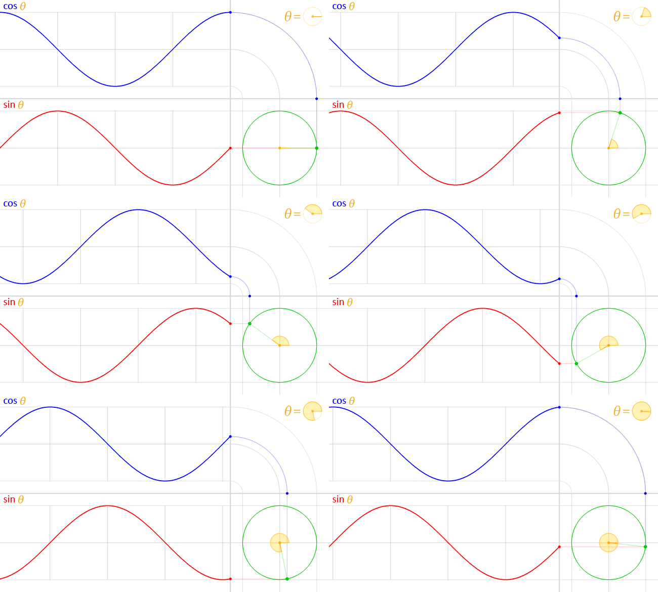
So we may want to imagine our electron as a pointlike electric charge (see the green dot in the illustration below) to spin around some center in either of the two possible directions. The cosine keeps track of the oscillation in one dimension, while the sine (plus or minus) keeps track of the oscillation in a direction that is perpendicular to the first one.

Figure 1: A pointlike charge in orbit

Circle_cos_sin

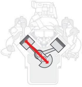
So we have a weird oscillator in two dimensions here, and we may calculate the energy in this oscillation. To calculate such energy, we need a mass concept. We only have a charge here, but a (moving) charge has an electromagnetic mass. Now, the electromagnetic mass of the electron’s charge may or may not explain all the mass of the electron (most physicists think it doesn’t) but let’s assume it does for the sake of the model that we’re trying to build up here. The point is: the theory of electromagnetic mass gives us a very simple explanation for the concept of mass here, and so we’ll use it for the time being. So we have some mass oscillating in two directions simultaneously: we basically assume space is, somehow, elastic. We have worked out the V-2 engine metaphor before, so we won’t repeat ourselves here.

Figure 2: A perpetuum mobile?

V2

Previously unrelated but structurally similar formulas may be related here:

  1. The energy of an oscillator: E = (1/2)·m·a2ω2
  2. Kinetic energy: E = (1/2)·m·v2
  3. The rotational (kinetic) energy that’s stored in a flywheel: E = (1/2)·I·ω2 = (1/2)·m·r2·ω2
  4. Einstein’s energy-mass equivalence relation: E = m·c2

Of course, we are mixing relativistic and non-relativistic formulas here, and there’s the 1/2 factor – but these are minor issues. For example, we were talking not one but two oscillators, so we should add their energies: (1/2)·m·a2·ω2 + (1/2)·m·a2·ω2 = m·a2·ω2. Also, one can show that the classical formula for kinetic energy (i.e. E = (1/2)·m·v2) morphs into E = m·c2 when we use the relativistically correct force equation for an oscillator. So, yes, our metaphor – or our suggested physical interpretation of the wavefunction, I should say – makes sense.

If you know something about physics, then you know the concept of the electromagnetic mass – its mathematical derivation, that is – gives us the classical electron radius, aka as the Thomson radius. It’s the smallest of a trio of radii that are relevant when discussing electrons: the other two radii are the Bohr radius and the Compton scattering radius respectively. The Thomson radius is used in the context of elastic scattering: the frequency of the incident particle (usually a photon), and the energy of the electron itself, do not change. In contrast, Compton scattering does change the frequency of the photon that is being scattered, and also impacts the energy of our electron. [As for the Bohr radius, you know that’s the radius of an electron orbital, roughly speaking – or the size of a hydrogen atom, I should say.]

Now, if we combine the E = m·a2·ω2 and E = m·c2 equations, then a·ω must be equal to c, right? Can we show this? Maybe. It is easy to see that we get the desired equality by substituting the amplitude of the oscillation (a) for the Compton scattering radius r = ħ/(m·c), and ω (the (angular) frequency of the oscillation) by using the Planck relation (ω = E/ħ):     

a·ω = [ħ/(m·c)]·[E/ħ] = E/(m·c) = m·c2/(m·c) = c

We get a wonderfully simple geometric model of an electron here: an electric charge that spins around in a plane. Its radius is the Compton electron radius – which makes sense – and the radial velocity of our spinning charge is the speed of light – which may or may not make sense. Of course, we need an explanation of why this spinning charge doesn’t radiate its energy away – but then we don’t have such explanation anyway. All we can say is that the electron charge seems to be spinning in its own space – that it’s racing along a geodesic. It’s just like mass creates its own space here: according to Einstein’s general relativity theory, gravity becomes a pseudo-force—literally: no real force. How? I am not sure: the model here assumes the medium – empty space – is, somehow, perfectly elastic: the electron constantly borrows energy from one direction and then returns it to the other – so to speak. A crazy model, yes – but is there anything better? We only want to present a metaphor here: a possible visualization of quantum-mechanical models.

However, if this model is to represent anything real, then many more questions need to be answered. For starters, let’s think about an interpretation of the results of the Stern-Gerlach experiment.

Precession

A spinning charge is a tiny magnet – and so it’s got a magnetic moment, which we need to explain the Stern-Gerlach experiment. But it doesn’t explain the discrete nature of the electron’s angular momentum: it’s either +ħ/2 or -ħ/2, nothing in-between, and that’s the case along any direction we choose. How can we explain this? Also, space is three-dimensional. Why would electrons spin in a perfect plane? The answer is: they don’t.

Indeed, the corollary of the above-mentioned binary value of the angular momentum is that the angular momentum – or the electron’s spin – is never completely along any direction. This may or may not be explained by the precession of a spinning charge in a field, which is illustrated below (illustration taken from Feynman’s Lectures, II-35-3).

Figure 3: Precession of an electron in a magnetic fieldprecession

So we do have an oscillation in three dimensions here, really – even if our wavefunction is a two-dimensional mathematical object. Note that the measurement (or the Stein-Gerlach apparatus in this case) establishes a line of sight and, therefore, a reference frame, so ‘up’ and ‘down’, ‘left’ and ‘right’, and ‘in front’ and ‘behind’ get meaning. In other words, we establish a real space. The question then becomes: how and why does an electron sort of snap into place?

The geometry of the situation suggests the logical angle of the angular momentum vector should be 45°. Now, if the value of its z-component (i.e. its projection on the z-axis) is to be equal to ħ/2, then the magnitude of J itself should be larger. To be precise, it should be equal to ħ/√2 ≈ 0.7·ħ (just apply Pythagoras’ Theorem). Is that value compatible with our flywheel model?

Maybe. Let’s see. The classical formula for the magnetic moment is μ = I·A, with I the (effective) current and A the (surface) area. The notation is confusing because I is also used for the moment of inertia, or rotational mass, but… Well… Let’s do the calculation. The effective current is the electron charge (qe) divided by the period (T) of the orbital revolution: : I = qe/T. The period of the orbit is the time that is needed for the electron to complete one loop. That time (T) is equal to the circumference of the loop (2π·a) divided by the tangential velocity (vt). Now, we suggest vt = r·ω = a·ω = c, and the circumference of the loop is 2π·a. For a, we still use the Compton radius a = ħ/(m·c). Now, the formula for the area is A = π·a2, so we get:

μ = I·A = [qe/T]·π·a2 = [qe·c/(2π·a)]·[π·a2] = [(qe·c)/2]·a = [(qe·c)/2]·[ħ/(m·c)] = [qe/(2m)]·ħ

In a classical analysis, we have the following relation between angular momentum and magnetic moment:

μ = (qe/2m)·J

Hence, we find that the angular momentum J is equal to ħ, so that’s twice the measured value. We’ve got a problem. We would have hoped to find ħ/2 or ħ/√2. Perhaps it’s  because a = ħ/(m·c) is the so-called reduced Compton scattering radius…

Well… No.

Maybe we’ll find the solution one day. I think it’s already quite nice we have a model that’s accurate up to a factor of 1/2 or 1/√2. 😊

Post scriptum: I’ve turned this into a small article which may or may not be more readable. You can link to it here. Comments are more than welcome.

Some content on this page was disabled on June 16, 2020 as a result of a DMCA takedown notice from The California Institute of Technology. You can learn more about the DMCA here:

https://wordpress.com/support/copyright-and-the-dmca/

Playing with amplitudes

Pre-script (dated 26 June 2020): This post got mutilated by the removal of some material by the dark force. You should be able to follow the main story line, however. If anything, the lack of illustrations might actually help you to think things through for yourself. In any case, we now have different views on these concepts as part of our realist interpretation of quantum mechanics, so we recommend you read our recent papers instead of these old blog posts.

Original post:

Let’s play a bit with the stuff we found in our previous post. This is going to be unconventional, or experimental, if you want. The idea is to give you… Well… Some ideas. So you can play yourself. 🙂 Let’s go.

Let’s first look at Feynman’s (simplified) formula for the amplitude of a photon to go from point a to point b. If we identify point a by the position vector r1 and point b by the position vector r2, and using Dirac’s fancy bra-ket notation, then it’s written as:

propagator

So we have a vector dot product here: p∙r12 = |p|∙|r12|· cosθ = p∙r12·cosα. The angle here (α) is the angle between the p and r12 vector. All good. Well… No. We’ve got a problem. When it comes to calculating probabilities, the α angle doesn’t matter: |ei·θ/r|2 = 1/r2. Hence, for the probability, we get: P = | 〈r2|r1〉 |2 = 1/r122. Always ! Now that’s strange. The θ = p∙r12/ħ argument gives us a different phase depending on the angle (α) between p and r12. But… Well… Think of it: cosα goes from 1 to 0 when α goes from 0 to ±90° and, of course, is negative when p and r12 have opposite directions but… Well… According to this formula, the probabilities do not depend on the direction of the momentum. That’s just weird, I think. Did Feynman, in his iconic Lectures, give us a meaningless formula?

Maybe. We may also note this function looks like the elementary wavefunction for any particle, which we wrote as:

ψ(x, t) = a·e−i∙θ = a·e−i∙(E∙t − p∙x)/ħ= a·e−i∙(E∙t)/ħ·ei∙(p∙x)/ħ

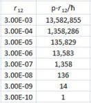
The only difference is that the 〈r2|r1〉 sort of abstracts away from time, so… Well… Let’s get a feel for the quantities. Let’s think of a photon carrying some typical amount of energy. Hence, let’s talk visible light and, therefore, photons of a few eV only – say 5.625 eV = 5.625×1.6×10−19 J = 9×10⁻¹⁹ J. Hence, their momentum is equal to p = E/c = (9×10⁻¹⁹ N·m)/(3×105 m/s) = 3×10⁻²⁴ N·s. That’s tiny but that’s only because newtons and seconds are enormous units at the (sub-)atomic scale. As for the distance, we may want to use the thickness of a playing card as a starter, as that’s what Young used when establishing the experimental fact of light interfering with itself. Now, playing cards in Young’s time were obviously rougher than those today, but let’s take the smaller distance: modern cards are as thin as 0.3 mm. Still, that distance is associated with a value of θ that is equal to 13.6 million. Hence, the density of our wavefunction is enormous at this scale, and it’s a bit of a miracle that Young could see any interference at all ! As shown in the table below, we only get meaningful values (remember: θ is a phase angle) when we go down to the nanometer scale (10−9 m) or, even better, the angstroms scale ((10−9 m). table action

So… Well… Again: what can we do with Feynman’s formula? Perhaps he didn’t give us a propagator function but something that is more general (read: more meaningful) at our (limited) level of knowledge. As I’ve been reading Feynman for quite a while now – like three or four years 🙂 – I think… Well… Yes. That’s it. Feynman wants us to think about it. 🙂 Are you joking again, Mr. Feynman? 🙂 So let’s assume the reasonable thing: let’s assume it gives us the amplitude to go from point a to point b by the position vector along some path r. So, then, in line with what we wrote in our previous post, let’s say p·r (momentum over a distance) is the action (S) we’d associate with this particular path (r) and then see where we get. So let’s write the formula like this:

ψ = a·ei·θ = (1/r)·ei·S/ħ = ei·p∙r/ħ/r

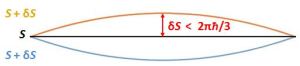
We’ll use an index to denote the various paths: r0 is the straight-line path and ri is any (other) path. Now, quantum mechanics tells us we should calculate this amplitude for every possible path. The illustration below shows the straight-line path and two nearby paths. So each of these paths is associated with some amount of action, which we measure in Planck units: θ = S/ħ. alternative paths

The time interval is given by t = t0 = r0/c, for all paths. Why is the time interval the same for all paths? Because we think of a photon going from some specific point in space and in time to some other specific point in space and in time. Indeed, when everything is said and done, we do think of light as traveling from point a to point b at the speed of light (c). In fact, all of the weird stuff here is all about trying to explain how it does that. 🙂

Now, if we would think of the photon actually traveling along this or that path, then this implies its velocity along any of the nonlinear paths will be larger than c, which is OK. That’s just the weirdness of quantum mechanics, and you should actually not think of the photon actually traveling along one of these paths anyway although we’ll often put it that way. Think of something fuzzier, whatever that may be. 🙂

So the action is energy times time, or momentum times distance. Hence, the difference in action between two paths i and j is given by:

δS = p·rj − p·ri = p·(rj − ri) = p·Δr

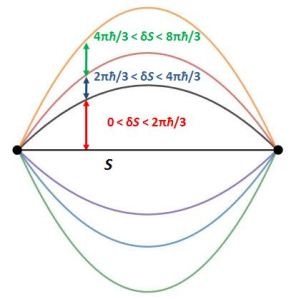
I’ll explain the δS < 2πħ/3 thing in a moment. Let’s first pause and think about the uncertainty and how we’re modeling it. We can effectively think of the variation in S as some uncertainty in the action: δS = ΔS = p·Δr. However, if S is also equal to energy times time (S = E·t), and we insist t is the same for all paths, then we must have some uncertainty in the energy, right? Hence, we can write δS as ΔS = ΔE·t. But, of course, E = E = m·c2 = p·c, so we will have an uncertainty in the momentum as well. Hence, the variation in S should be written as:

δS = ΔS = Δp·Δr

That’s just logical thinking: if we, somehow, entertain the idea of a photon going from some specific point in spacetime to some other specific point in spacetime along various paths, then the variation, or uncertainty, in the action will effectively combine some uncertainty in the momentum and the distance. We can calculate Δp as ΔE/c, so we get the following:

δS = ΔS = Δp·Δr = ΔE·Δr/c = ΔE·Δt with Δt = Δr/c

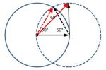
So we have the two expressions for the Uncertainty Principle here: ΔS = Δp·Δr = ΔE·Δt. Just be careful with the interpretation of Δt: it’s just the equivalent of Δr. We just express the uncertainty in distance in seconds using the (absolute) speed of light. We are not changing our spacetime interval: we’re still looking at a photon going from a to b in t seconds, exactly. Let’s now look at the δS < 2πħ/3 thing. If we’re adding two amplitudes (two arrows or vectors, so to speak) and we want the magnitude of the result to be larger than the magnitude of the two contributions, then the angle between them should be smaller than 120 degrees, so that’s 2π/3 rad. The illustration below shows how you can figure that out geometrically.angles 2Hence, if S0 is the action for r0, then S1 = S0 + ħ and S2 = S0 + 2·ħ are still good, but S3 = S0 + 3·ħ is not good. Why? Because the difference in the phase angles is Δθ = S1/ħ − S0/ħ = (S0 + ħ)/ħ − S0/ħ = 1 and Δθ = S2/ħ − S0/ħ = (S0 + 2·ħ)/ħ − S0/ħ = 2 respectively, so that’s 57.3° and 114.6° respectively and that’s, effectively, less than 120°. In contrast, for the next path, we find that Δθ = S3/ħ − S0/ħ = (S0 + 3·ħ)/ħ − S0/ħ = 3, so that’s 171.9°. So that amplitude gives us a negative contribution.

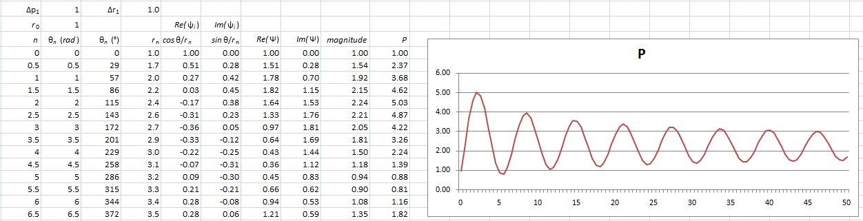
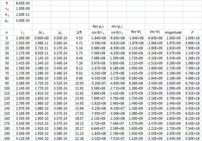
Let’s do some calculations using a spreadsheet. To simplify things, we will assume we measure everything (time, distance, force, mass, energy, action,…) in Planck units. Hence, we can simply write: Sn = S0 + n. Of course, n = 1, 2,… etcetera, right? Well… Maybe not. We are measuring action in units of ħ, but do we actually think action comes in units of ħ? I am not sure. It would make sense, intuitively, but… Well… There’s uncertainty on the energy (E) and the momentum (p) of our photon, right? And how accurately can we measure the distance? So there’s some randomness everywhere. 😦 So let’s leave that question open as for now.

We will also assume that the phase angle for S0 is equal to 0 (or some multiple of 2π, if you want). That’s just a matter of choosing the origin of time. This makes it really easy: ΔSn = Sn − S0 = n, and the associated phase angle θn = Δθn is the same. In short, the amplitude for each path reduces to ψn = ei·n/r0. So we need to add these first and then calculate the magnitude, which we can then square to get a probability. Of course, there is also the issue of normalization (probabilities have to add up to one) but let’s tackle that later. For the calculations, we use Euler’s r·ei·θ = r·(cosθ + i·sinθ) = r·cosθ + i·r·sinθ formula. Needless to say, |r·ei·θ|2 = |r|2·|ei·θ|2 = |r|2·(cos2θ + sin2θ) = r. Finally, when adding complex numbers, we add the real and imaginary parts respectively, and we’ll denote the ψ0 + ψ1 +ψ2 + … sum as Ψ.

Now, we also need to see how our ΔS = Δp·Δr works out. We may want to assume that the uncertainty in p and in r will both be proportional to the overall uncertainty in the action. For example, we could try writing the following: ΔSn = Δpn·Δrn = n·Δp1·Δr1. It also makes sense that you may want Δpn and Δrn to be proportional to Δp1 and Δr1 respectively. Combining both, the assumption would be this:

Δpn = √n·Δp1 and Δrn = √n·Δr1

So now we just need to decide how we will distribute ΔS1 = ħ = 1 over Δp1 and Δr1 respectively. For example, if we’d assume Δp1 = 1, then Δr1 = ħ/Δp1 = 1/1 = 1. These are the calculations. I will let you analyze them. 🙂newnewWell… We get a weird result. It reminds me of Feynman’s explanation of the partial reflection of light, shown below, but… Well… That doesn’t make much sense, does it?

partial reflection

Hmm… Maybe it does. 🙂 Look at the graph more carefully. The peaks sort of oscillate out so… Well… That might make sense… 🙂

Does it? Are we doing something wrong here? These amplitudes should reflect the ones that are reflected in those nice animations (like this one, for example, which is part of that’s part of the Wikipedia article on Feynman’s path integral formulation of quantum mechanics). So what’s wrong, if anything? Well… Our paths differ by some fixed amount of action, which doesn’t quite reflect the geometric approach that’s used in those animations. The graph below shows how the distance r varies as a function of n. geometry

If we’d use a model in which the distance would increase linearly or, preferably, exponentially, then we’d get the result we want to get, right?

Well… Maybe. Let’s try it. Hmm… We need to think about the geometry here. Look at the triangle below. triangle sideIf b is the straight-line path (r0), then ac could be one of the crooked paths (rn). To simplify, we’ll assume isosceles triangles, so a equals c and, hence, rn = 2·a = 2·c. We will also assume the successive paths are separated by the same vertical distance (h = h1) right in the middle, so hb = hn = n·h1. It is then easy to show the following:r formulaThis gives the following graph for rn = 10 and h1 = 0.01.r graph

Is this the right step increase? Not sure. We can vary the values in our spreadsheet. Let’s first build it. The photon will have to travel faster in order to cover the extra distance in the same time, so its momentum will be higher. Let’s think about the velocity. Let’s start with the first path (n = 1). In order to cover the extra distance Δr1, the velocity c1 must be equal to (r0 + Δr1)/t = r0/t + Δr1/t = c + Δr1/t = c0 + Δr1/t. We can write c1 as c1 = c0 + Δc1, so Δc1 = Δr1/t. Now, the ratio of p1  and p0 will be equal to the ratio of c1 and c0 because p1/p0 = (mc1)/mc0) = c1/c0. Hence, we have the following formula for p1:

p1 = p0·c1/c0 = p0·(c0 + Δc1)/c0 = p0·[1 + Δr1/(c0·t) = p0·(1 + Δr1/r0)

For pn, the logic is the same, so we write:

pn = p0·cn/c0 = p0·(c0 + Δcn)/c0 = p0·[1 + Δrn/(c0·t) = p0·(1 + Δrn/r0)

Let’s do the calculations, and let’s use meaningful values, so the nanometer scale and actual values for Planck’s constant and the photon momentum. The results are shown below. original

Pretty interesting. In fact, this looks really good. The probability first swings around wildly, because of these zones of constructive and destructive interference, but then stabilizes. [Of course, I would need to normalize the probabilities, but you get the idea, right?] So… Well… I think we get a very meaningful result with this model. Sweet ! 🙂 I’m lovin’ it ! 🙂 And, here you go, this is (part of) the calculation table, so you can see what I am doing. 🙂newnew

The graphs below look even better: I just changed the h1/r0 ratio from 1/100 to 1/10. The probability stabilizes almost immediately. 🙂 So… Well… It’s not as fancy as the referenced animation, but I think the educational value of this thing here is at least as good ! 🙂great

🙂 This is good stuff… 🙂

Post scriptum (19 September 2017): There is an obvious inconsistency in the model above, and in the calculations. We assume there is a path r1 = , r2, r2,etcetera, and then we calculate the action for it, and the amplitude, and then we add the amplitude to the sum. But, surely, we should count these paths twice, in two-dimensional space, that is. Think of the graph: we have positive and negative interference zones that are sort of layered around the straight-line path, as shown below.zones

In three-dimensional space, these lines become surfaces. Hence, rather than adding one arrow for every δ  having one contribution only, we may want to add… Well… In three-dimensional space, the formula for the surface around the straight-line path would probably look like π·hn·r1, right? Hmm… Interesting idea. I changed my spreadsheet to incorporate that idea, and I got the graph below. It’s a nonsensical result, because the probability does swing around, but it gradually spins out of control: it never stabilizes.revisedThat’s because we increase the weight of the paths that are further removed from the center. So… Well… We shouldn’t be doing that, I guess. 🙂 I’ll you look for the right formula, OK? Let me know when you found it. 🙂

Some content on this page was disabled on June 16, 2020 as a result of a DMCA takedown notice from The California Institute of Technology. You can learn more about the DMCA here:

https://wordpress.com/support/copyright-and-the-dmca/

The energy and 1/2 factor in Schrödinger’s equation

Schrödinger’s equation, for a particle moving in free space (so we have no external force fields acting on it, so V = 0 and, therefore, the Vψ term disappears) is written as:

∂ψ(x, t)/∂t = i·(1/2)·(ħ/meff)·∇2ψ(x, t)

We already noted and explained the structural similarity with the ubiquitous diffusion equation in physics:

∂φ(x, t)/∂t = D·∇2φ(x, t) with x = (x, y, z)

The big difference between the wave equation and an ordinary diffusion equation is that the wave equation gives us two equations for the price of one: ψ is a complex-valued function, with a real and an imaginary part which, despite their name, are both equally fundamental, or essential. Whatever word you prefer. 🙂 That’s also what the presence of the imaginary unit (i) in the equation tells us. But for the rest it’s the same: the diffusion constant (D) in Schrödinger’s equation is equal to (1/2)·(ħ/meff).

Why the 1/2 factor? It’s ugly. Think of the following: If we bring the (1/2)·(ħ/meff) to the other side, we can write it as meff/(ħ/2). The ħ/2 now appears as a scaling factor in the diffusion constant, just like ħ does in the de Broglie equations: ω = E/ħ and k = p/ħ, or in the argument of the wavefunction: θ = (E·t − p∙x)/ħ. Planck’s constant is, effectively, a physical scaling factor. As a physical scaling constant, it usually does two things:

  1. It fixes the numbers (so that’s its function as a mathematical constant).
  2. As a physical constant, it also fixes the physical dimensions. Note, for example, how the 1/ħ factor in ω = E/ħ and k = p/ħ ensures that the ω·t = (E/ħ)·t and k·x = (p/ħ)·x terms in the argument of the wavefunction are both expressed as some dimensionless number, so they can effectively be added together. Physicists don’t like adding apples and oranges.

The question is: why did Schrödinger use ħ/2, rather than ħ, as a scaling factor? Let’s explore the question.

The 1/2 factor

We may want to think that 1/2 factor just echoes the 1/2 factor in the Uncertainty Principle, which we should think of as a pair of relations: σx·σp ≥ ħ/2 and σE·σt ≥ ħ/2. However, the 1/2 factor in those relations only makes sense because we chose to equate the fundamental uncertainty (Δ) in x, p, E and t with the mathematical concept of the standard deviation (σ), or the half-width, as Feynman calls it in his wonderfully clear exposé on it in one of his Lectures on quantum mechanics (for a summary with some comments, see my blog post on it). We may just as well choose to equate Δ with the full-width of those probability distributions we get for x and p, or for E and t. If we do that, we get σx·σp ≥ ħ and σE·σt ≥ ħ.

It’s a bit like measuring the weight of a person on an old-fashioned (non-digital) bathroom scale with 1 kg marks only: do we say this person is x kg ± 1 kg, or x kg ± 500 g? Do we take the half-width or the full-width as the margin of error? In short, it’s a matter of appreciation, and the 1/2 factor in our pair of uncertainty relations is not there because we’ve got two relations. Likewise, it’s not because I mentioned we can think of Schrödinger’s equation as a pair of relations that, taken together, represent an energy propagation mechanism that’s quite similar in its structure to Maxwell’s equations for an electromagnetic wave (as shown below), that we’d insert (or not) that 1/2 factor: either of the two representations below works. It just depends on our definition of the concept of the effective mass.

The 1/2 factor is really a matter of choice, because the rather peculiar – and flexible – concept of the effective mass takes care of it. However, we could define some new effective mass concept, by writing: meffNEW = 2∙meffOLD, and then Schrödinger’s equation would look more elegant:

∂ψ/∂t = i·(ħ/meffNEW)·∇2ψ

Now you’ll want the definition, of course! What is that effective mass concept? Feynman talks at length about it, but his exposé is embedded in a much longer and more general argument on the propagation of electrons in a crystal lattice, which you may not necessarily want to go through right now. So let’s try to answer that question by doing something stupid: let’s substitute ψ in the equation for ψ = a·e−i·[E·t − p∙x]/ħ (which is an elementary wavefunction), calculate the time derivative and the Laplacian, and see what we get. If we do that, the ∂ψ/∂t = i·(1/2)·(ħ/meff)·∇2ψ equation becomes:

−i·a·(E/ħ)·e−i∙(E·t − p∙x)/ħ = −i·a·(1/2)·(ħ/meff)(p2/ħ2)·e−i∙(E·t − p∙x)/ħ 

⇔ E = (1/2)·p2/meff = (1/2)·(m·v)2/meff ⇔ meff = (1/2)·(m/E)·m·v2

⇔ meff = (1/c2)·(m·v2/2) = m·β2/2

Hence, the effective mass appears in this equation as the equivalent mass of the kinetic energy (K.E.) of the elementary particle that’s being represented by the wavefunction. Now, you may think that sounds good – and it does – but you should note the following:

1. The K.E. = m·v2/2 formula is only correct for non-relativistic speeds. In fact, it’s the kinetic energy formula if, and only if, if m ≈ m0. The relativistically correct formula for the kinetic energy calculates it as the difference between (1) the total energy (which is given by the E = m·c2 formula, always) and (2) its rest energy, so we write:

K.E. = E − E0 = mv·c2 − m0·c2 = m0·γ·c2 − m0·c2 = m0·c2·(γ − 1)

2. The energy concept in the wavefunction ψ = a·e−i·[E·t − p∙x]/ħ is, obviously, the total energy of the particle. For non-relativistic speeds, the kinetic energy is only a very small fraction of the total energy. In fact, using the formula above, you can calculate the ratio between the kinetic and the total energy: you’ll find it’s equal to 1 − 1/γ = 1 − √(1−v2/c2), and its graph goes from 0 to 1.

graph

Now, if we discard the 1/2 factor, the calculations above yield the following:

−i·a·(E/ħ)·e−i∙(E·t − p∙x)/ħ = −i·a·(ħ/meff)(p2/ħ2)·e−i∙(E·t − p∙x)/ħ 

⇔ E = p2/meff = (m·v)2/meff ⇔ meff = (m/E)·m·v2

⇔ meff = m·v2/c2 = m·β2

In fact, it is fair to say that both definitions are equally weird, even if the dimensions come out alright: the effective mass is measured in old-fashioned mass units, and the β2 or β2/2 factor appears as a sort of correction factor, varying between 0 and 1 (for β2) or between 0 and 1/2 (for β2/2). I prefer the new definition, as it ensures that meff becomes equal to m in the limit for the velocity going to c. In addition, if we bring the ħ/meff or (1/2)∙ħ/meff factor to the other side of the equation, the choice becomes one between a meffNEW/ħ or a 2∙meffOLD/ħ coefficient.

It’s a choice, really. Personally, I think the equation without the 1/2 factor – and, hence, the use of ħ rather than ħ/2 as the scaling factor – looks better, but then you may argue that – if half of the energy of our particle is in the oscillating real part of the wavefunction, and the other is in the imaginary part – then the 1/2 factor should stay, because it ensures that meff becomes equal to m/2 as v goes to c (or, what amounts to the same, β goes to 1). But then that’s the argument about whether or not we should have a 1/2 factor because we get two equations for the price of one, like we did for the Uncertainty Principle.

So… What to do? Let’s first ask ourselves whether that derivation of the effective mass actually makes sense. Let’s therefore look at both limit situations.

1. For v going to c (or β = v/c going to 1), we do not have much of a problem: meff just becomes the total mass of the particle that we’re looking at, and Schrödinger’s equation can easily be interpreted as an energy propagation mechanism. Our particle has zero rest mass in that case ( we may also say that the concept of a rest mass is meaningless in this situation) and all of the energy – and, therefore, all of the equivalent mass – is kinetic: m = E/c2 and the effective mass is just the mass: meff = m·c2/c2 = m. Hence, our particle is everywhere and nowhere. In fact, you should note that the concept of velocity itself doesn’t make sense in this rather particular case. It’s like a photon (but note it’s not a photon: we’re talking some theoretical particle here with zero spin and zero rest mass): it’s a wave in its own frame of reference, but as it zips by at the speed of light, we think of it as a particle.

2. Let’s look at the other limit situation. For v going to 0 (or β = v/c going to 0), Schrödinger’s equation no longer makes sense, because the diffusion constant goes to zero, so we get a nonsensical equation. Huh? What’s wrong with our analysis?

Well… I must be honest. We started off on the wrong foot. You should note that it’s hard – in fact, plain impossible – to reconcile our simple a·e−i·[E·t − p∙x]/ħ function with the idea of the classical velocity of our particle. Indeed, the classical velocity corresponds to a group velocity, or the velocity of a wave packet, and so we just have one wave here: no group. So we get nonsense. You can see the same when equating p to zero in the wave equation: we get another nonsensical equation, because the Laplacian is zero! Check it. If our elementary wavefunction is equal to ψ = a·e−i·(E/ħ)·t, then that Laplacian is zero.

Hence, our calculation of the effective mass is not very sensical. Why? Because the elementary wavefunction is a theoretical concept only: it may represent some box in space, that is uniformly filled with energy, but it cannot represent any actual particle. Actual particles are always some superposition of two or more elementary waves, so then we’ve got a wave packet (as illustrated below) that we can actually associate with some real-life particle moving in space, like an electron in some orbital indeed. 🙂

wave-packet

I must credit Oregon State University for the animation above. It’s quite nice: a simple particle in a box model without potential. As I showed on my other page (explaining various models), we must add at least two waves – traveling in opposite directions – to model a particle in a box. Why? Because we represent it by a standing wave, and a standing wave is the sum of two waves traveling in opposite directions.

So, if our derivation above was not very meaningful, then what is the actual concept of the effective mass?

The concept of the effective mass

I am afraid that, at this point, I do have to direct you back to the Grand Master himself for the detail. Let me just try to sum it up very succinctly. If we have a wave packet, there is – obviously – some energy in it, and it’s energy we may associate with the classical concept of the velocity of our particle – because it’s the group velocity of our wave packet. Hence, we have a new energy concept here – and the equivalent mass, of course. Now, Feynman’s analysis – which is Schrödinger’s analysis, really – shows we can write that energy as:

E = meff·v2/2

So… Well… That’s the classical kinetic energy formula. And it’s the very classical one, because it’s not relativistic. 😦 But that’s OK for relatively small-moving electrons! [Remember the typical (relative) velocity is given by the fine-structure constant: α = β = v/c. So that’s impressive (about 2,188 km per second), but it’s only a tiny fraction of the speed of light, so non-relativistic formulas should work.]

Now, the meff factor in this equation is a function of the various parameters of the model he uses. To be precise, we get the following formula out of his model (which, as mentioned above, is a model of electrons propagating in a crystal lattice):

meff = ħ2/(2·A·b2 )

Now, the b in this formula is the spacing between the atoms in the lattice. The A basically represents an energy barrier: to move from one atom to another, the electron needs to get across it. I talked about this in my post on it, and so I won’t explain the graph below – because I did that in that post. Just note that we don’t need that factor 2: there is no reason whatsoever to write E0 + 2·A and E0 − 2·A. We could just re-define a new A: (1/2)·ANEW = AOLD. The formula for meff then simplifies to ħ2/(2·AOLD·b2) = ħ2/(ANEW·b2). We then get an Eeff = meff·v2 formula for the extra energy.

energy

Eeff = meff·v2?!? What energy formula is that? Schrödinger must have thought the same thing, and so that’s why we have that ugly 1/2 factor in his equation. However, think about it. Our analysis shows that it is quite straightforward to model energy as a two-dimensional oscillation of mass. In this analysis, both the real and the imaginary component of the wavefunction each store half of the total energy of the object, which is equal to E = m·c2. Remember, indeed, that we compared it to the energy in an oscillator, which is equal to the sum of kinetic and potential energy, and for which we have the T + U = m·ω02/2 formula. But so we have two oscillators here and, hence, twice the energy. Hence, the E = m·c2 corresponds to m·ω02 and, hence, we may think of c as the natural frequency of the vacuum.

Therefore, the Eeff = meff·v2 formula makes much more sense. It nicely mirrors Einstein’s E = m·c2 formula and, in fact, naturally merges into E = m·c2  for v approaching c. But, I admit, it is not so easy to interpret. It’s much easier to just say that the effective mass is the mass of our electron as it appears in the kinetic energy formula, or – alternatively – in the momentum formula. Indeed, Feynman also writes the following formula:

meff·v = p = ħ·k

Now, that is something we easily recognize! 🙂

So… Well… What do we do now? Do we use the 1/2 factor or not?

It would be very convenient, of course, to just stick with tradition and use meff as everyone else uses it: it is just the mass as it appears in whatever medium we happen to look it, which may be a crystal lattice (or a semi-conductor), or just free space. In short, it’s the mass of the electron as it appears to us, i.e. as it appears in the (non-relativistic) kinetic energy formula (K.E. = meff·v2/2), the formula for the momentum of an electron (p = meff·v), or in the wavefunction itself (k = p/ħ = (meff·v)/ħ. In fact, in his analysis of the electron orbitals, Feynman (who just follows Schrödinger here) drops the eff subscript altogether, and so the effective mass is just the mass: meff = m. Hence, the apparent mass of the electron in the hydrogen atom serves as a reference point, and the effective mass in a different medium (such as a crystal lattice, rather than free space or, I should say, a hydrogen atom in free space) will also be different.

The thing is: we get the right results out of Schrödinger’s equation, with the 1/2 factor in it. Hence, Schrödinger’s equation works: we get the actual electron orbitals out of it. Hence, Schrödinger’s equation is true – without any doubt. Hence, if we take that 1/2 factor out, then we do need to use the other effective mass concept. We can do that. Think about the actual relation between the effective mass and the real mass of the electron, about which Feynman writes the following: “The effective mass has nothing to do with the real mass of an electron. It may be quite different—although in commonly used metals and semiconductors it often happens to turn out to be the same general order of magnitude: about 0.1 to 30 times the free-space mass of the electron.” Hence, if we write the relation between meff and m as meff = g(m), then the same relation for our meffNEW = 2∙meffOLD becomes meffNEW = 2·g(m), and the “about 0.1 to 30 times” becomes “about 0.2 to 60 times.”

In fact, in the original 1963 edition, Feynman writes that the effective mass is “about 2 to 20 times” the free-space mass of the electron. Isn’t that interesting? I mean… Note that factor 2! If we’d write meff = 2·m, then we’re fine. We can then write Schrödinger’s equation in the following two equivalent ways:

  1. (meff/ħ)·∂ψ/∂t = i·∇2ψ
  2. (2m/ħ)·∂ψ/∂t = i·∇2ψ

Both would be correct, and it explains why Schrödinger’s equation works. So let’s go for that compromise and write Schrödinger’s equation in either of the two equivalent ways. 🙂 The question then becomes: how to interpret that factor 2? The answer to that question is, effectively, related to the fact that we get two waves for the price of one here. So we have two oscillators, so to speak. Now that‘s quite deep, and I will explore that in one of my next posts.

Let me now address the second weird thing in Schrödinger’s equation: the energy factor. I should be more precise: the weirdness arises when solving Schrödinger’s equation. Indeed, in the texts I’ve read, there is this constant switching back and forth between interpreting E as the energy of the atom, versus the energy of the electron. Now, both concepts are obviously quite different, so which one is it really?

The energy factor E

It’s a confusing point—for me, at least and, hence, I must assume for students as well. Let me indicate, by way of example, how the confusion arises in Feynman’s exposé on the solutions to the Schrödinger equation. Initially, the development is quite straightforward. Replacing V by −e2/r, Schrödinger’s equation becomes:

Eq1

As usual, it is then assumed that a solution of the form ψ (r, t) =  e−(i/ħ)·E·t·ψ(r) will work. Apart from the confusion that arises because we use the same symbol, ψ, for two different functions (you will agree that ψ (r, t), a function in two variables, is obviously not the same as ψ(r), a function in one variable only), this assumption is quite straightforward and allows us to re-write the differential equation above as:

de

To get this, you just need to actually to do that time derivative, noting that the ψ in our equation is now ψ(r), not ψ (r, t). Feynman duly notes this as he writes: “The function ψ(r) must solve this equation, where E is some constant—the energy of the atom.” So far, so good. In one of the (many) next steps, we re-write E as E = ER·ε, with ER = m·e4/2ħ2. So we just use the Rydberg energy (ER ≈ 13.6 eV) here as a ‘natural’ atomic energy unit. That’s all. No harm in that.

Then all kinds of complicated but legitimate mathematical manipulations follow, in an attempt to solve this differential equation—attempt that is successful, of course! However, after all these manipulations, one ends up with the grand simple solution for the s-states of the atom (i.e. the spherically symmetric solutions):

En = −ER/n2 with 1/n2 = 1, 1/4, 1/9, 1/16,…, 1

So we get: En = −13.6 eV, −3.4 eV, −1.5 eV, etcetera. Now how is that possible? How can the energy of the atom suddenly be negative? More importantly, why is so tiny in comparison with the rest energy of the proton (which is about 938 mega-electronvolt), or the electron (0.511 MeV)? The energy levels above are a few eV only, not a few million electronvolt. Feynman answers this question rather vaguely when he states the following:

“There is, incidentally, nothing mysterious about negative numbers for the energy. The energies are negative because when we chose to write V = −e2/r, we picked our zero point as the energy of an electron located far from the proton. When it is close to the proton, its energy is less, so somewhat below zero. The energy is lowest (most negative) for n = 1, and increases toward zero with increasing n.”

We picked our zero point as the energy of an electron located far away from the proton? But we were talking the energy of the atom all along, right? You’re right. Feynman doesn’t answer the question. The solution is OK – well, sort of, at least – but, in one of those mathematical complications, there is a ‘normalization’ – a choice of some constant that pops up when combining and substituting stuff – that is not so innocent. To be precise, at some point, Feynman substitutes the ε variable for the square of another variable – to be even more precise, he writes: ε = −α2. He then performs some more hat tricks – all legitimate, no doubt – and finds that the only sensible solutions to the differential equation require α to be equal to 1/n, which immediately leads to the above-mentioned solution for our s-states.

The real answer to the question is given somewhere else. In fact, Feynman casually gives us an explanation in one of his very first Lectures on quantum mechanics, where he writes the following:

“If we have a “condition” which is a mixture of two different states with different energies, then the amplitude for each of the two states will vary with time according to an equation like a·e−iωt, with ħ·ω = E0 = m·c2. Hence, we can write the amplitude for the two states, for example as:

e−i(E1/ħ)·t and e−i(E2/ħ)·t

And if we have some combination of the two, we will have an interference. But notice that if we added a constant to both energies, it wouldn’t make any difference. If somebody else were to use a different scale of energy in which all the energies were increased (or decreased) by a constant amount—say, by the amount A—then the amplitudes in the two states would, from his point of view, be

e−i(E1+A)·t/ħ and e−i(E2+A)·t/ħ

All of his amplitudes would be multiplied by the same factor e−i(A/ħ)·t, and all linear combinations, or interferences, would have the same factor. When we take the absolute squares to find the probabilities, all the answers would be the same. The choice of an origin for our energy scale makes no difference; we can measure energy from any zero we want. For relativistic purposes it is nice to measure the energy so that the rest mass is included, but for many purposes that aren’t relativistic it is often nice to subtract some standard amount from all energies that appear. For instance, in the case of an atom, it is usually convenient to subtract the energy Ms·c2, where Ms is the mass of all the separate pieces—the nucleus and the electrons—which is, of course, different from the mass of the atom. For other problems, it may be useful to subtract from all energies the amount Mg·c2, where Mg is the mass of the whole atom in the ground state; then the energy that appears is just the excitation energy of the atom. So, sometimes we may shift our zero of energy by some very large constant, but it doesn’t make any difference, provided we shift all the energies in a particular calculation by the same constant.”

It’s a rather long quotation, but it’s important. The key phrase here is, obviously, the following: “For other problems, it may be useful to subtract from all energies the amount Mg·c2, where Mg is the mass of the whole atom in the ground state; then the energy that appears is just the excitation energy of the atom.” So that’s what he’s doing when solving Schrödinger’s equation. However, I should make the following point here: if we shift the origin of our energy scale, it does not make any difference in regard to the probabilities we calculate, but it obviously does make a difference in terms of our wavefunction itself. To be precise, its density in time will be very different. Hence, if we’d want to give the wavefunction some physical meaning – which is what I’ve been trying to do all along – it does make a huge difference. When we leave the rest mass of all of the pieces in our system out, we can no longer pretend we capture their energy.

This is a rather simple observation, but one that has profound implications in terms of our interpretation of the wavefunction. Personally, I admire the Great Teacher’s Lectures, but I am really disappointed that he doesn’t pay more attention to this. 😦

Freewheeling…

In my previous post, I copied a simple animation from Wikipedia to show how one can move from Cartesian to polar coordinates. It’s really neat. Just watch it a few times to appreciate what’s going on here.

Cartesian_to_polarFirst, the function is being inverted, so we go from y = f(x) to x = g(y) with g = f−1. In this case, we know that if y = sin(6x) + 2 (that’s the function above), then x = (1/6)·arcsin(y – 2). [Note the troublesome convention to denote the inverse function by the -1 superscript: it’s troublesome because that superscript is also used for a reciprocal—and f−1 has, obviously, nothing to do with 1/f. In any case, let’s move on.] So we swap the x-axis for the y-axis, and vice versa. In fact, to be precise, we reflect them about the diagonal. In fact, w’re reflecting the whole space here, including the graph of the function. Note that, in three-dimensional space, this reflection can also be looked at as a rotation – again, of all space, including the graph and the axes  – by 180 degrees. The axis of rotation is, obviously, the same diagonal. [I like how the animation visualizes this. Neat! It made me think!]

Of course, if we swap the axes, then the domain and the range of the function get swapped too. Let’s see how that works here: x goes from −π to +π, so that’s one cycle (but one that starts from −π and goes to +π, rather than from 0 to 2π), and, hence, y ranges between 1 and 3. [Whatever its argument, the sine function always yields a value between −1 and +1, but we add 2 to every value it takes, so we get the [1, 3] interval now.] After swapping the x- and y-axis, the angle, i.e. the interval between −π and +π, is now on the vertical axis. That’s clear enough. So far so good. 🙂 The operation that follows, however, is a much more complicated transformation of space and, therefore, much more interesting.

The transformation bends the graph around the origin so its head and tail meet. That’s easy to see. What’s a bit more difficult to understand is how the coordinate axes transform. I had to look at the animation several times – so please do the same. Note how this transformation wraps all of the vertical lines around a circle, and how the radius of those  circles depends on the distance of those lines from the origin (as measured along the horizontal axis). What about the vertical axis? The animation is somewhat misleading here, as it gives the impression we’re first making another circle out of it, which we then sort of shrink—all the way down to a circle with zero radius! So the vertical axis becomes the origin of our new space. However, there’s no shrinking really. What happens is that we also wrap it around a circle—but one with zero radius indeed!

It’s a very weird operation because we’re dealing with a non-linear transformation here (unlike rotation or reflection) and, therefore, we’re not familiar with it. Even weirder is what happens to the horizontal axis: somehow, this axis becomes an infinite disc, so the distance out is now measured from the center outwards. I should figure out the math here, but that’s for later. The point is: the r = sin(6θ) + 2 function in the final graph (i.e. the curve that looks like a petaled flower) is the same as that y = sin(6x) + 2 curve, so y = r and x = θ, and so we can write what’s written above: r(θ) = sin(6·θ) + 2.

You’ll say: nice, but so what? Well… When I saw this animation, my first reaction was: what if the x and y would be time and space respectively? You’ll say: what space? Well… Just space: three-dimensional space. So think of one of the axes as packing three dimensions really, or three directions—like what’s depicted below. Now think of some point-like object traveling through spacetime, as shown below. It doesn’t need to be point-like, of course—just small enough so we can represent its trajectory by a line. You can also think of the movement of its center-of-mass if you don’t like point-like assumptions. 🙂

trajectory

Of course, you’ll immediately say the trajectory above is not kosher, as our object travels back in time in three sections of this ‘itinerary’.

You’re right. Let’s correct that. It’s easy to see how we should correct it. We just need to ensure the itinerary is a well-defined function, which isn’t the case with the function above: for one value of t, we have only one value of x everywhere—except where we allow our particle to travel back in time. So… Well… We shouldn’t allow that. The concept of a well-defined function implies we need to choose one direction in time. 🙂 That’s neat, because this gives us an explanation for the unique direction of time without having to invoke entropy or other macro-concepts. So let’s replace that thing above by something more kosher traveling in spacetime, like the thing below.

trajectory 2Now think of wrapping that around some circle. We’d get something like below. [Don’t worry about the precise shape of the  graph, as I made up a new one. Note the remark on the need to have a well-behaved function applies here too!]

trajectory 4Neat, you’ll say, but so what? All we’ve done so far is show that we can represent some itinerary in spacetime in two different ways. In the first representation, we measure time along some linear axis, while, in the second representation, time becomes some angle—an angle that increases, counter-clockwise. To put it differently: time becomes an angular velocity.

Likewise, the spatial dimension was a linear feature in the first representation, while in the second we think of it as some distance measured from some zero point. Well… In fact… No. That’s not correct. The r above has got nothing to do with the distance traveled: the distance traveled would need to be measured along the curve.

Hmm… What’s the deal here?

Frankly, I am not sure. Now that I look at it once more, I note that the exercise with our graph above involved one cycle of a periodic function only—so it’s really not like some object traveling in spacetime, because that’s not a periodic thing. But… Well… Does that matter all that much? It’s easy to imagine how our new representation would just involve some thing that keeps going around and around, as illustrated below.

trajectory 5

So, in this representation, any movement in spacetime – regular or irregular – does become something periodic. But what is periodic here? My first answer is the simplest and, hence, probably the correct one: it’s just time. Time is the periodic thing here.

Having said that, I immediately thought of something else that’s periodic: the wavefunction that’s associated with this object—any object traveling in spacetime, really—is periodic too. So my guts instinct tells me there’s something here that we might want to explore further. 🙂 Could we replace the function for the trajectory with the wavefunction?

Huh? Yes. The wavefunction also associates each x and t, although the association is a bit more complex—literally, because we’ll associate it with two periodic functions: the real part and the imaginary part of the (complex-valued) wavefunction. But for the rest, no problem, I’d say. Remember our wavefunction, when squared, represents the probability of our object being there. [I should say “absolute-squared” rather than squared, but that sounds so weird.]

But… Yes? Well… Don’t we get in trouble here because the same complex number (i.e. r·eθ = x + i·y) may be related to two points in spacetime—as shown in the example above? My answer is the same: I don’t think so. It’s the same thing: our new representation implies stuff keeps going around and around in it. In fact, that just captures the periodicity of the wavefunction. So… Well… It’s fine. 🙂

The more important question is: what can we do with this new representation? Here I do not have any good answer. Nothing much for the moment. I just wanted to jot it down, because it triggers some deep thoughts—things I don’t quite understand myself, as yet.

First, I like the connection between a regular trajectory in spacetime – as represented by a well-defined function – and the unique direction in time it implies. It’s a simple thing: we know something can travel in any direction in space – forward, backwards, sideways, whatever – but time has one direction only. At least we can see why now: both in Cartesian as well as polar coordinates, we’d want to see a well-behaved function. 🙂 Otherwise we couldn’t work with it.

Another thought is the following. We associate the momentum of a particle with a linear trajectory in spacetime. But what’s linear in curved spacetime? Remember how we struggle to represent – or imagine, I would say – curved spacetime, as evidenced by the fact that most illustrations of curved spacetime represent a two-dimensional space in three-dimensional Cartesian space? Think of the typical illustration, like that rubber surface with the ball deforming it.

That’s why this transformation of a Cartesian coordinate space into a polar coordinate space is such an interesting exercise. We now measure distance along the circle. [Note that we suddenly need to keep track of the number of rotations, which we can do by keeping track of time, as time units become some angle, and linear speed becomes angular speed.] The whole thing underscores, in my view, that’s it’s only our mind that separates time and space: the reality of the object is just its movement or velocity – and that’s one movement.

My guts instinct tells me that this is what the periodicity of the wavefunction (or its component waves, I should say) captures, somehow. If the movement is linear, it’s linear both in space as well in time, so to speak:

  • As a mental construct, time is always linear – it goes in one direction (and we think of the clock being regular, i.e. not slowing down or speeding up) – and, hence, the mathematical qualities of the time variable in the wavefunction are the same as those of the position variable: it’s a factor in one of its two terms. To be precise, it appears as the t in the E·t term in the argument θ = E·t – p·x. [Note the minus sign appears because we measure angles counter-clockwise when using polar coordinates or complex numbers.]
  • The trajectory in space is also linear – whether or not space is curved because of the presence of other masses.

OK. I should conclude here, but I want take this conversation one step further. Think of the two graphs below as representing some oscillation in space. Some object that goes back and forth in space: it accelerates and decelerates—and reverses direction. Imagine the g-forces on it as it does so: if you’d be traveling with that object, you would sure feel it’s going back and forth in space! The graph on the left-hand side is our usual perspective on stuff like this: we measure time using some steadily ticking clock, and so the seconds, minutes, hours, days, etcetera just go by.graph 1

The graph on the right-hand side applies our inversion technique. But, frankly, it’s the same thing: it doesn’t give us any new information. It doesn’t look like a well-behaved function but it actually is. It’s just a matter of mathematical convention: if we’d be used to looking at the y-axis as the independent variable (rather than the dependent variable), the function would be acceptable.

This leads me to the idea I started to explore in my previous post, and that’s to try to think of wavefunctions as oscillations of spacetime, rather than oscillations in spacetime. I inserted the following graph in that post—but it doesn’t say all that much, as it suggests we’re doing the same thing here: we’re just swapping axes. The difference is that the θ in the first graph now combines both time and space. We might say it represents spacetime itself. So the wavefunction projects it into some other ‘space’, i.e. the complex space. And then in the second graph, we reflect the whole thing.

dependent independent

So the idea is the following: our functions sort of project one ‘space’ into another ‘space’. In this case: the wavefunction sort of transforms spacetime – i.e. what we like to think of as the ‘physical’ space – into a complex space – which is purely mathematical.

Hmm… This post is becoming way too long, so I need to wrap it up. Look at the graph below, and note the dimension of the axes. We’re looking at an oscillation once more, but an oscillation of time this time around.

Graph 2

Huh? Yes. Imagine that, for some reason, you don’t feel those g-forces while going up and down in space: it’s the rest of the world that’s moving. You think you’re stationary or—what amounts to the same according to the relativity principle—moving in a straight line at constant velocity. The only way how you could explain the rest of the world moving back and forth, accelerating and decelerating, is that time itself is oscillating: objects reverse their direction for no apparent reason—so that’s time reversal—and they do so a varying speeds, so we’ve got a clock going wild!

You’ll nod your head in agreement now and say: that’s Einstein’s intuition in regard to the gravitational force. There’s no force really: mass just bends spacetime in such a way a planet in orbit follows a straight line, in a curved spacetime continuum. What I am saying here is that there must be ways to think of the electromagnetic force in exactly the same way. If the accelerations and decelerations of an electron moving in some electron would really be due to an electromagnetic force in the classical picture of a force (i.e. something pulling or pushing), then it would radiate energy away. We know it doesn’t do that—because otherwise it would spiral down into the nucleus itself. So I’ve been thinking it must be traveling in its own curved spacetime, but then it’s curved because of the electromagnetic force—obviously, as that’s the force that’s much more relevant at this scale.

The underlying thought is simple enough: if gravity curves spacetime, why can’t we look at the other forces as doing the same? Why can’t we think of any force coming ‘with its own space’, so to say? The difference between the various forces is the curvature – which will, obviously, be much more complex (literally) for the electromagnetic force. Just think of the other forces as curving space in more than one dimension. 🙂

I am sure you’ll think I’ve just gone crazy. Perhaps. In any case, I don’t care too much. As mentioned, because the electromagnetic force is different—we don’t have negative masses attracting positive masses when discussing gravity—it’s going to be a much weirder type of curvature, but… Well… That’s probably why we need those ‘two-dimensional’ complex numbers when discussing quantum mechanics! 🙂 So we’ve got some more mathematical dimensions, but the physical principle behind all forces should be the same, no? All forces are measured using Newton’s Law, so we relate them to the motion of some mass. The principle is simple: if force is related to the change in motion of a mass, then the trajectory in the space that’s related to that force will be linear if the force is not acting.

So… Well… Hmm… What? 

All of what I write above is a bit of a play with words, isn’t it? An oscillation of spacetime—but then spacetime must oscillate in something else, doesn’it? So in what then is it oscillating?

Great question. You’re right. It must be oscillating in something else or, to be precise, we need some other reference space so as to define what we mean by an oscillation of spacetime. That space is going to be some complex mathematical space—and I use complex both in its mathematical as well as in its everyday meaning here (complicated). Think of, for example, that x-axis representing three-dimensional space. We’d have something similar here: dimensions within dimensions.

There’s some great videos on YouTube that illustrate how one can turn a sphere inside out without punching a hole in it. That’s basically what we’re talking about here: it’s more than just switching the range for the domain of a function, which we can do by that reflection – or mirroring – using the 45º line. Conceptually, it’s really like turning a sphere inside out. Think of the surface of the curve connecting the two spaces.

Huh? Yes. But… Well… You’re right. Stuff like this is for the graduate level, I guess. So I’ll let you think about it—and do watch the videos that follow it. 🙂

In any case, I have to stop my wandering about here. Rather than wrapping up, however, I thought of something else yesterday—and so I’ll quickly jot that down as well, so I can re-visit it some other time. 🙂

Some other thinking on the Uncertainty Principle

I wanted to jot down something else too here. Something about the Uncertainty Principle once more. In my previous post, I noted we should think of Planck’s constant as expressing itself in time or in space, as we have two ways of looking at the dimension of Planck’s constant:

  1. [Planck’s constant] = [ħ] = N∙m∙s = (N∙m)∙s = [energy]∙[time]
  2. [Planck’s constant] = [ħ] = N∙m∙s = (N∙s)∙m = [momentum]∙[distance]

The bracket symbols [ and ] mean: ‘the dimension of what’s between the brackets’. Now, this may look like kids stuff, but the idea is quite fundamental: we’re thinking here of some amount of action (ħ, i.e. the quantum of action) expressing itself in time or, alternatively, expressing itself in space, indeed. In the former case, some amount of energy is expended during some time. In the latter case, some momentum is expended over some distance. We also know ħ can be written in terms of fundamental units, which are referred to as Planck units:

ħ = FP∙lP∙tP = Planck force unit × Planck distance unit × Planck time unit

Finally, we thought of the Planck distance unit and the Planck time unit as the smallest units of time and distance possible. As such, they become countable variables, so we’re talking of a trajectory in terms of discrete steps in space and time here, or discrete states of our particle. As such, the E·t and p·x in the argument (θ) of the wavefunction—remember: θ = (E/ħ)·t − (p/ħ)·x—should be some multiple of ħ as well. We may write:

E·t = m·ħ and p·x = n·ħ, with m and n both positive integers

Of course, there’s uncertainty: Δp·Δx ≥ ħ/2 and ΔE·Δt ≥ ħ/2. Now, if Δx and Δt also become countable variables, so Δx and Δt can only take on values like ±1, ±2, ±3, ±4, etcetera, then we can think of trying to model some kind of random walk through spacetime, combining various values for n and m, as well as various values for Δx and Δt. The relation between E and p, and the related difference between m and n, should determine in what direction our particle should be moving even if it can go along different trajectories. In fact, Feynman’s path integral formulation of quantum mechanics tells us it’s likely to move along different trajectories at the same time, with each trajectory having its own amplitude. Feynman’s formulation uses continuum theory, of course, but a discrete analysis – using a random walk approach – should yield the same result because, when everything is said and done, the fact that physics tells us time and space must become countable at some scale (the Planck scale), suggests that continuum theory may not represent reality, but just be an approximation: a limiting situation, in other words.

Hmmm… Interesting… I’ll need to do something more with this. Unfortunately, I have little time over the coming weeks. Again, I am just  writing it down to re-visit it later—probably much later. 😦

The Uncertainty Principle

In my previous post, I showed how Feynman derives Schrödinger’s equation using a historical and, therefore, quite intuitive approach. The approach was intuitive because the argument used a discrete model, so that’s stuff we are well acquainted with—like a crystal lattice, for example. However, now we’re now going to think continuity from the start. Let’s first see what changes in terms of notation.

New notations

Our C(xn, t) = 〈xn|ψ〉 now becomes C(x) = 〈x|ψ〉. This notation does not explicitly show the time dependence but then you know amplitudes like this do vary in space as well as in time. Having said that, the analysis below focuses mainly on their behavior in space, so it does make sense to not explicitly mention the time variable. It’s the usual trick: we look at how stuff behaves in space or, alternatively, in time. So we temporarily ‘forget’ about the other variable. That’s just how we work: it’s hard for our mind to think about these wavefunctions in both dimensions simultaneously although, ideally, we should do that.

Now, you also know that quantum physicists prefer to denote the wavefunction C(x) with some Greek letter: ψ (psi) or φ (phi). Feynman think it’s somewhat confusing because we use the same to denote a state itself, but I don’t agree. I think it’s pretty straightforward. In any case, we write:

ψ(x) = Cψ(x) = C(x) = 〈x|ψ〉

The next thing is the associated probabilities. From your high school math course, you’ll surely remember that we have two types of probability distributions: they are either discrete or, else, continuous. If they’re continuous, then our probability distribution becomes a probability density function (PDF) and, strictly speaking, we should no longer say that the probability of finding our particle at any particular point x at some time t is this or that. That probability is, strictly speaking, zero: if our variable is continuous, then our probability is defined for an interval only, and the P[x] value itself is referred to as a probability density. So we’ll look at little intervals Δx, and we can write the associated probability as:

prob (x, Δx) = |〈x|ψ〉|2Δx = |ψ(x)|2Δx

The idea is illustrated below. We just re-divide our continuous scale in little intervals and calculate the surface of some tiny elongated rectangle now. 🙂

image024

It is also easy to see that, when moving to an infinite set of states, our 〈φ|ψ〉 = ∑〈φ|x〉〈x|ψ〉 (over all x) formula for calculating the amplitude for a particle to go from state ψ to state φ should now be written as an infinite sum, i.e. as the following integral:

amplitude continuous

Now, we know that 〈φ|x〉 = 〈x|φ〉* and, therefore, this integral can also be written as:

integral

For example, if φ(x) =  〈x|φ〉 is equal to a simple exponential, so we can write φ(x) = a·e−iθ, then φ*(x) =  〈φ|x〉 = a·e+iθ.

With that, we’re ready for the plat de résistance, except for one thing, perhaps: we don’t look at spin here. If we’d do that, we’d have to take two sets of base sets: one for up and one for down spin—but we don’t worry about this, for the time being, that is. 🙂

The momentum wavefunction

Our wavefunction 〈x|ψ〉 varies in time as well as in space. That’s obvious. How exactly depends on the energy and the momentum: both are related and, hence, if there’s uncertainty in the momentum, there will be uncertainty in the momentum, and vice versa. Uncertainty in the momentum changes the behavior of the wavefunction in space—through the p = ħk factor in the argument of the wavefunction (θ = ω·t − k·x)—while uncertainty in the energy changes the behavior of the wavefunction in time—through the E = ħω relation. As mentioned above, we focus on the variation in space here. We’ll do so y defining a new state, which is referred to as a state of definite momentum. We’ll write it as mom p, and so now we can use the Dirac notation to write the amplitude for an electron to have a definite momentum equal to p as:

φ(p) = 〈 mom p | ψ 〉

Now, you may think that the 〈x|ψ〉 and 〈mom p|ψ〉 amplitudes should be the same because, surely, we do associate the x state with a definite momentum p, don’t we? Well… No! If we want to localize our wave ‘packet’, i.e. localize our particle, then we’re actually not going to associate it with a definite momentum. See my previous posts: we’re going to introduce some uncertainty so our wavefunction is actually a superposition of more elementary waves with slightly different (spatial) frequencies. So we should just go through the motions here and apply our integral formula to ‘unpack’ this amplitude. That goes as follows:

integral 2

So, as usual, when seeing a formula like this, we should remind ourselves of what we need to solve. Here, we assume we somehow know the ψ(x) = 〈x|ψ〉 wavefunction, so the question is: what do we use for 〈 mom p | x 〉? At this point, Feynman wanders off to start a digression on normalization, which really confuses the picture. When everything is said and done, the easiest thing to do is to just jot down the formula for that 〈mom p | x〉 in the integrand and think about it for a while:

〈mom p | x〉 = e−i(p/ħ)∙x

I mean… What else could it be? This formula is very fundamental, and I am not going to try to explain it. As mentioned above, Feynman tries to ‘explain’ it by some story about probabilities and normalization, but I think his ‘explanation’ just confuses things even more. Really, what else would it be? The formula above really encapsulates what it means if we say that p and x are conjugate variables. [I can already note, of course, that symmetry implies that we can write something similar for energy and time. Indeed, we can define a state of definite energy as 〈E | ψ〉, and then ‘unpack’ it in the same way, and see that one of the two factors in the integrand would be equal to 〈E | t〉 and, of course, we’d associate a similar formula with it:

〈E | t〉 = ei(E/ħ)∙t

But let me get back to the lesson here. We’re analyzing stuff in space now, not in time. Feynman gives a simple example here. He suggests a wavefunction which has the following form:

ψ(x) = K·e−x2/4σ2

The example is somewhat disingenuous because this is not a complex– but real-valued function. In fact, squaring it, and then calculating K applying the normalization condition (all probabilities have to add up to one), yields the normal probability distribution:

prob (x, Δx) = P(x)dx = (2πσ2)−1/2e−x2/2σ2dx

So that’s just the normal distribution for μ = 0, as illustrated below.

720px-Normal_Distribution_PDF

In any case, the integral we have to solve now is:Integral 3

Now, I hate integrals as much as you do (probably more) and so I assume you’re also only interested in the result (if you want the detail: check it in Feynman), which we can write as:

φ(p) = (2πη2)−1/4·e−p2/4η2, with η = ħ/2σ

This formula is totally identical to the ψ(x) = (2πσ2)−1/4·e−x2/4σ2 distribution we started with, except that it’s got another sigma value, which we denoted by η (and that’s not nu but eta), with 

η = ħ/2σ

Just for the record, Feynman refers to η and σ as the ‘half-width’ of the respective distributions. Mathematicians would say they’re the standard deviation. The concept are nearly the same, but not quite. In any case, that’s another thing I’ll let you find our for yourself. 🙂 The point is: η and σ are inversely proportional to each other, and the constant of proportionality is equal to ħ/2.

Now, if we take η and σ as measures of the uncertainty in p and x respectively – which is what they are, obviously ! – then we can re-write that η = ħ/2σ as ησ = ħ/2 or, better still, as the Uncertainty Principle itself:

ΔpΔx = ħ/2

You’ll say: that’s great, but we usually see the Uncertainty Principle written as:

ΔpΔx ≥ ħ/2

So where does that come from? Well… We choose a normal distribution (or the Gaussian distribution, as physicists call it), and so that yields the ΔpΔx = ħ/2 identity. If we’d chosen another one, we’d find a slightly different relation and so… Well… Let me quote Feynman here: “Interestingly enough, it is possible to prove that for any other form of a distribution in x or p, the product ΔpΔx cannot be smaller than the one we have found here, so the Gaussian distribution gives the smallest possible value for the ΔpΔx product.”

This is great. So what about the even more approximate ΔpΔx ≥ ħ formula? Where does that come from? Well… That’s more like a qualitative version of it: it basically says the minimum value of the same product is of the same order as ħ which, as you know, is pretty tiny: it’s about 0.0000000000000000000000000000000006626 J·s. 🙂 The last thing to note is its dimension: momentum is expressed in newton-second and position in meter, obviously. So the uncertainties in them are expressed in the same unit, and so the dimension of the product is N·m·s = J·s. So this dimension combines force, distance and time. That’s quite appropriate, I’d say. The ΔEΔt product obviously does the same. But… Well… That’s it, folks! I enjoyed writing this – and I cannot always say the same of other posts! So I hope you enjoyed reading it. 🙂

Some content on this page was disabled on June 16, 2020 as a result of a DMCA takedown notice from The California Institute of Technology. You can learn more about the DMCA here:

https://wordpress.com/support/copyright-and-the-dmca/
Some content on this page was disabled on June 16, 2020 as a result of a DMCA takedown notice from The California Institute of Technology. You can learn more about the DMCA here:

https://wordpress.com/support/copyright-and-the-dmca/

The de Broglie relations, the wave equation, and relativistic length contraction

Pre-script (dated 26 June 2020): Our ideas have evolved into a full-blown realistic (or classical) interpretation of all things quantum-mechanical. So no use to read this. Read my recent papers instead. 🙂

Original post:

You know the two de Broglie relations, also known as matter-wave equations:

f = E/h and λ = h/p

You’ll find them in almost any popular account of quantum mechanics, and the writers of those popular books will tell you that f is the frequency of the ‘matter-wave’, and λ is its wavelength. In fact, to add some more weight to their narrative, they’ll usually write them in a somewhat more sophisticated form: they’ll write them using ω and k. The omega symbol (using a Greek letter always makes a big impression, doesn’t it?) denotes the angular frequency, while k is the so-called wavenumber.  Now, k = 2π/λ and ω = 2π·f and, therefore, using the definition of the reduced Planck constant, i.e. ħ = h/2π, they’ll write the same relations as:

  1. λ = h/p = 2π/k ⇔ k = 2π·p/h
  2. f = E/h = (ω/2π)

⇒ k = p/ħ and ω = E/ħ

They’re the same thing: it’s just that working with angular frequencies and wavenumbers is more convenient, from a mathematical point of view that is: it’s why we prefer expressing angles in radians rather than in degrees (k is expressed in radians per meter, while ω is expressed in radians per second). In any case, the ‘matter wave’ – even Wikipedia uses that term now – is, of course, the amplitude, i.e. the wave-function ψ(x, t), which has a frequency and a wavelength, indeed. In fact, as I’ll show in a moment, it’s got two frequencies: one temporal, and one spatial. I am modest and, hence, I’ll admit it took me quite a while to fully distinguish the two frequencies, and so that’s why I always had trouble connecting these two ‘matter wave’ equations.

Indeed, if they represent the same thing, they must be related, right? But how exactly? It should be easy enough. The wavelength and the frequency must be related through the wave velocity, so we can write: f·λ = v, with v the velocity of the wave, which must be equal to the classical particle velocity, right? And then momentum and energy are also related. To be precise, we have the relativistic energy-momentum relationship: p·c = mv·v·c = mv·c2·v/c = E·v/c. So it’s just a matter of substitution. We should be able to go from one equation to the other, and vice versa. Right?

Well… No. It’s not that simple. We can start with either of the two equations but it doesn’t work. Try it. Whatever substitution you try, there’s no way you can derive one of the two equations above from the other. The fact that it’s impossible is evidenced by what we get when we’d multiply both equations. We get:

  1. f·λ = (E/h)·(h/p) = E/p
  2. v = f·λ  ⇒ f·λ = v = E/p ⇔ E = v·p = v·(m·v)

⇒ E = m·v2

Huh? What kind of formula is that? E = m·v2? That’s a formula you’ve never ever seen, have you? It reminds you of the kinetic energy formula of course—K.E. = m·v2/2—but… That factor 1/2 should not be there. Let’s think about it for a while. First note that this E = m·v2 relation makes perfectly sense if v = c. In that case, we get Einstein’s mass-energy equivalence (E = m·c2), but that’s besides the point here. The point is: if v = c, then our ‘particle’ is a photon, really, and then the E = h·f is referred to as the Planck-Einstein relation. The wave velocity is then equal to c and, therefore, f·λ = c, and so we can effectively substitute to find what we’re looking for:

E/p = (h·f)/(h/λ) = f·λ = c ⇒ E = p·c 

So that’s fine: we just showed that the de Broglie relations are correct for photons. [You remember that E = p·c relation, no? If not, check out my post on it.] However, while that’s all nice, it is not what the de Broglie equations are about: we’re talking the matter-wave here, and so we want to do something more than just re-confirm that Planck-Einstein relation, which you can interpret as the limit of the de Broglie relations for v = c. In short, we’re doing something wrong here! Of course, we are. I’ll tell you what exactly in a moment: it’s got to do with the fact we’ve got two frequencies really.

Let’s first try something else. We’ve been using the relativistic E = mv·c2 equation above. Let’s try some other energy concept: let’s substitute the E in the f = E/h by the kinetic energy and then see where we get—if anywhere at all. So we’ll use the Ekinetic = m∙v2/2 equation. We can then use the definition of momentum (p = m∙v) to write E = p2/(2m), and then we can relate the frequency f to the wavelength λ using the v = λ∙f formula once again. That should work, no? Let’s do it. We write:

  1. E = p2/(2m)
  2. E = h∙f = h·v/λ

⇒ λ = h·v/E = h·v/(p2/(2m)) = h·v/[m2·v2/(2m)] = h/[m·v/2] = 2∙h/p

So we find λ = 2∙h/p. That is almost right, but not quite: that factor 2 should not be there. Well… Of course you’re smart enough to see it’s just that factor 1/2 popping up once more—but as a reciprocal, this time around. 🙂 So what’s going on? The honest answer is: you can try anything but it will never work, because the f = E/h and λ = h/p equations cannot be related—or at least not so easily. The substitutions above only work if we use that E = m·v2 energy concept which, you’ll agree, doesn’t make much sense—at first, at least. Again: what’s going on? Well… Same honest answer: the f = E/h and λ = h/p equations cannot be related—or at least not so easily—because the wave equation itself is not so easy.

Let’s review the basics once again.

The wavefunction

The amplitude of a particle is represented by a wavefunction. If we have no information whatsoever on its position, then we usually write that wavefunction as the following complex-valued exponential:

ψ(x, t) = a·e−i·[(E/ħ)·t − (p/ħ)∙x] = a·e−i·(ω·t − k∙x) = a·ei(k∙x−ω·t) = a·eiθ = a·(cosθ + i·sinθ)

θ is the so-called phase of our wavefunction and, as you can see, it’s the argument of a wavefunction indeed, with temporal frequency ω and spatial frequency k (if we choose our x-axis so its direction is the same as the direction of k, then we can substitute the k and x vectors for the k and x scalars, so that’s what we’re doing here). Now, we know we shouldn’t worry too much about a, because that’s just some normalization constant (remember: all probabilities have to add up to one). However, let’s quickly develop some logic here. Taking the absolute square of this wavefunction gives us the probability of our particle being somewhere in space at some point in time. So we get the probability as a function of x and t. We write:

P(x ,t) = |a·e−i·[(E/ħ)·t − (p/ħ)∙x]|2 = a2

As all probabilities have to add up to one, we must assume we’re looking at some box in spacetime here. So, if the length of our box is Δx = x2 − x1, then (Δx)·a2 = (x2−x1)·a2 = 1 ⇔ Δx = 1/a2. [We obviously simplify the analysis by assuming a one-dimensional space only here, but the gist of the argument is essentially correct.] So, freezing time (i.e. equating t to some point t = t0), we get the following probability density function:

Capture

That’s simple enough. The point is: the two de Broglie equations f = E/h and λ = h/p give us the temporal and spatial frequencies in that ψ(x, t) = a·e−i·[(E/ħ)·t − (p/ħ)∙x] relation. As you can see, that’s an equation that implies a much more complicated relationship between E/ħ = ω and p/ħ = k. Or… Well… Much more complicated than what one would think of at first.

To appreciate what’s being represented here, it’s good to play a bit. We’ll continue with our simple exponential above, which also illustrates how we usually analyze those wavefunctions: we either assume we’re looking at the wavefunction in space at some fixed point in time (t = t0) or, else, at how the wavefunction changes in time at some fixed point in space (x = x0). Of course, we know that Einstein told us we shouldn’t do that: space and time are related and, hence, we should try to think of spacetime, i.e. some ‘kind of union’ of space and time—as Minkowski famously put it. However, when everything is said and done, mere mortals like us are not so good at that, and so we’re sort of condemned to try to imagine things using the classical cut-up of things. 🙂 So we’ll just an online graphing tool to play with that a·ei(k∙x−ω·t) = a·eiθ = a·(cosθ + i·sinθ) formula.

Compare the following two graps, for example. Just imagine we either look at how the wavefunction behaves at some point in space, with the time fixed at some point t = t0, or, alternatively, that we look at how the wavefunction behaves in time at some point in space x = x0. As you can see, increasing k = p/ħ or increasing ω = E/ħ gives the wavefunction a higher ‘density’ in space or, alternatively, in time.

density 1

density 2That makes sense, intuitively. In fact, when thinking about how the energy, or the momentum, affects the shape of the wavefunction, I am reminded of an airplane propeller: as it spins, faster and faster, it gives the propeller some ‘density’, in space as well as in time, as its blades cover more space in less time. It’s an interesting analogy: it helps—me, at least—to think through what that wavefunction might actually represent.

propeller

So as to stimulate your imagination even more, you should also think of representing the real and complex part of that ψ = a·ei(k∙x−ω·t) = a·eiθ = a·(cosθ + i·sinθ) formula in a different way. In the graphs above, we just showed the sine and cosine in the same plane but, as you know, the real and the imaginary axis are orthogonal, so Euler’s formula a·eiθ = a·(cosθ + i·sinθ) = a·cosθ + i·a·sinθ = Re(ψ) + i·Im(ψ) may also be graphed as follows:
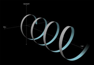
5d_euler_f

The illustration above should make you think of yet another illustration you’ve probably seen like a hundred times before: the electromagnetic wave, propagating through space as the magnetic and electric field induce each other, as illustrated below. However, there’s a big difference: Euler’s formula incorporates a phase shift—remember: sinθ = cos(θ − π/2)—and you don’t have that in the graph below. The difference is much more fundamental, however: it’s really hard to see how one could possibly relate the magnetic and electric field to the real and imaginary part of the wavefunction respectively. Having said that, the mathematical similarity makes one think!

FG02_06

Of course, you should remind yourself of what E and B stand for: they represent the strength of the electric (E) and magnetic (B) field at some point x at some time t. So you shouldn’t think of those wavefunctions above as occupying some three-dimensional space. They don’t. Likewise, our wavefunction ψ(x, t) does not occupy some physical space: it’s some complex number—an amplitude that’s associated with each and every point in spacetime. Nevertheless, as mentioned above, the visuals make one think and, as such, do help us as we try to understand all of this in a more intuitive way.

Let’s now look at that energy-momentum relationship once again, but using the wavefunction, rather than those two de Broglie relations.

Energy and momentum in the wavefunction

I am not going to talk about uncertainty here. You know that Spiel. If there’s uncertainty, it’s in the energy or the momentum, or in both. The uncertainty determines the size of that ‘box’ (in spacetime) in which we hope to find our particle, and it’s modeled by a splitting of the energy levels. We’ll say the energy of the particle may be E0, but it might also be some other value, which we’ll write as En = E0 ± n·ħ. The thing to note is that energy levels will always be separated by some integer multiple of ħ, so ħ is, effectively , the quantum of energy for all practical—and theoretical—purposes. We then super-impose the various wave equations to get a wave function that might—or might not—resemble something like this:
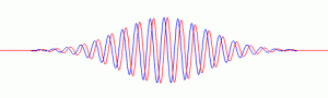
Photon waveWho knows? 🙂 In any case, that’s not what I want to talk about here. Let’s repeat the basics once more: if we write our wavefunction a·e−i·[(E/ħ)·t − (p/ħ)∙x] as a·e−i·[ω·t − k∙x], we refer to ω = E/ħ as the temporal frequency, i.e. the frequency of our wavefunction in time (i.e. the frequency it has if we keep the position fixed), and to k = p/ħ as the spatial frequency (i.e. the frequency of our wavefunction in space (so now we stop the clock and just look at the wave in space). Now, let’s think about the energy concept first. The energy of a particle is generally thought of to consist of three parts:

  1. The particle’s rest energy m0c2, which de Broglie referred to as internal energy (Eint): it includes the rest mass of the ‘internal pieces’, as Feynman puts it (now we call those ‘internal pieces’ quarks), as well as their binding energy (i.e. the quarks’ interaction energy);
  2. Any potential energy it may have because of some field (so de Broglie was not assuming the particle was traveling in free space), which we’ll denote by U, and note that the field can be anything—gravitational, electromagnetic: it’s whatever changes the energy because of the position of the particle;
  3. The particle’s kinetic energy, which we write in terms of its momentum p: m·v2/2 = m2·v2/(2m) = (m·v)2/(2m) = p2/(2m).

So we have one energy concept here (the rest energy) that does not depend on the particle’s position in spacetime, and two energy concepts that do depend on position (potential energy) and/or how that position changes because of its velocity and/or momentum (kinetic energy). The two last bits are related through the energy conservation principle. The total energy is E = mvc2, of course—with the little subscript (v) ensuring the mass incorporates the equivalent mass of the particle’s kinetic energy.

So what? Well… In my post on quantum tunneling, I drew attention to the fact that different potentials , so different potential energies (indeed, as our particle travels one region to another, the field is likely to vary) have no impact on the temporal frequency. Let me re-visit the argument, because it’s an important one. Imagine two different regions in space that differ in potential—because the field has a larger or smaller magnitude there, or points in a different direction, or whatever: just different fields, which corresponds to different values for U1 and U2, i.e. the potential in region 1 versus region 2. Now, the different potential will change the momentum: the particle will accelerate or decelerate as it moves from one region to the other, so we also have a different p1 and p2. Having said that, the internal energy doesn’t change, so we can write the corresponding amplitudes, or wavefunctions, as:

  1. ψ1(θ1) = Ψ1(x, t) = a·e−iθ1 = a·e−i[(Eint + p12/(2m) + U1)·t − p1∙x]/ħ 
  2. ψ2(θ2) = Ψ2(x, t) = a·e−iθ2 = a·e−i[(Eint + p22/(2m) + U2)·t − p2∙x]/ħ 

Now how should we think about these two equations? We are definitely talking different wavefunctions. However, their temporal frequencies ω1 = Eint + p12/(2m) + U1 and ω1 = Eint + p22/(2m) + U2 must be the same. Why? Because of the energy conservation principle—or its equivalent in quantum mechanics, I should say: the temporal frequency f or ω, i.e. the time-rate of change of the phase of the wavefunction, does not change: all of the change in potential, and the corresponding change in kinetic energy, goes into changing the spatial frequency, i.e. the wave number k or the wavelength λ, as potential energy becomes kinetic or vice versa. The sum of the potential and kinetic energy doesn’t change, indeed. So the energy remains the same and, therefore, the temporal frequency does not change. In fact, we need this quantum-mechanical equivalent of the energy conservation principle to calculate how the momentum and, hence, the spatial frequency of our wavefunction, changes. We do so by boldly equating ω1 = Eint + p12/(2m) + U1 and ω2 = Eint + p22/(2m) + U2, and so we write:

ω1 = ω2 ⇔ Eint + p12/(2m) + U1 =  Eint + p22/(2m) + U2 

⇔ p12/(2m) − p22/(2m) = U2 – U1 ⇔ p22 =  (2m)·[p12/(2m) – (U2 – U1)]

⇔ p2 = (p12 – 2m·ΔU )1/2

We played with this in a previous post, assuming that p12 is larger than 2m·ΔU, so as to get a positive number on the right-hand side of the equation for p22, so then we can confidently take the positive square root of that (p12 – 2m·ΔU ) expression to calculate p2. For example, when the potential difference ΔU = U2 – U1 was negative, so ΔU < 0, then we’re safe and sure to get some real positive value for p2.

Having said that, we also contemplated the possibility that p22 = p12 – 2m·ΔU was negative, in which case p2 has to be some pure imaginary number, which we wrote as p2 = i·p’ (so p’ (read: p prime) is a real positive number here). We could work with that: it resulted in an exponentially decreasing factor e−p’·x/ħ that ended up ‘killing’ the wavefunction in space. However, its limited existence still allowed particles to ‘tunnel’ through potential energy barriers, thereby explaining the quantum-mechanical tunneling phenomenon.

This is rather weird—at first, at least. Indeed, one would think that, because of the E/ħ = ω equation, any change in energy would lead to some change in ω. But no! The total energy doesn’t change, and the potential and kinetic energy are like communicating vessels: any change in potential energy is associated with a change in p, and vice versa. It’s a really funny thing. It helps to think it’s because the potential depends on position only, and so it should not have an impact on the temporal frequency of our wavefunction. Of course, it’s equally obvious that the story would change drastically if the potential would change with time, but… Well… We’re not looking at that right now. In short, we’re assuming energy is being conserved in our quantum-mechanical system too, and so that implies what’s described above: no change in ω, but we obviously do have changes in p whenever our particle goes from one region in space to another, and the potentials differ. So… Well… Just remember: the energy conservation principle implies that the temporal frequency of our wave function doesn’t change. Any change in potential, as our particle travels from one place to another, plays out through the momentum.

Now that we know that, let’s look at those de Broglie relations once again.

Re-visiting the de Broglie relations

As mentioned above, we usually think in one dimension only: we either freeze time or, else, we freeze space. If we do that, we can derive some funny new relationships. Let’s first simplify the analysis by re-writing the argument of the wavefunction as:

θ = E·t − p·x

Of course, you’ll say: the argument of the wavefunction is not equal to E·t − p·x: it’s (E/ħ)·t − (p/ħ)∙x. Moreover, θ should have a minus sign in front. Well… Yes, you’re right. We should put that 1/ħ factor in front, but we can change units, and so let’s just measure both E as well as p in units of ħ here. We can do that. No worries. And, yes, the minus sign should be there—Nature choose a clockwise direction for θ—but that doesn’t matter for the analysis hereunder.

The E·t − p·x expression reminds one of those invariant quantities in relativity theory. But let’s be precise here. We’re thinking about those so-called four-vectors here, which we wrote as pμ = (E, px, py, pz) = (E, p) and xμ = (t, x, y, z) = (t, x) respectively. [Well… OK… You’re right. We wrote those four-vectors as pμ = (E, px·c , py·c, pz·c) = (E, p·c) and xμ = (c·t, x, y, z) = (t, x). So what we write is true only if we measure time and distance in equivalent units so we have c = 1. So… Well… Let’s do that and move on.] In any case, what was invariant was not E·t − p·x·c or c·t − x (that’s a nonsensical expression anyway: you cannot subtract a vector from a scalar), but pμ2 = pμpμ = E2 − (p·c)2 = E2 − p2·c2 = E2 − (px2 + py2 + pz2)·c2 and xμ2 = xμxμ = (c·t)2 − x2 = c2·t2 − (x2 + y2 + z2) respectively. [Remember pμpμ and xμxμ are four-vector dot products, so they have that +— signature, unlike the p2 and x2 or a·b dot products, which are just a simple sum of the squared components.] So… Well… E·t − p·x is not an invariant quantity. Let’s try something else.

Let’s re-simplify by equating ħ as well as c to one again, so we write: ħ = c = 1. [You may wonder if it is possible to ‘normalize’ both physical constants simultaneously, but the answer is yes. The Planck unit system is an example.]  then our relativistic energy-momentum relationship can be re-written as E/p = 1/v. [If c would not be one, we’d write: E·β = p·c, with β = v/c. So we got E/p = c/β. We referred to β as the relative velocity of our particle: it was the velocity, but measured as a ratio of the speed of light. So here it’s the same, except that we use the velocity symbol v now for that ratio.]

Now think of a particle moving in free space, i.e. without any fields acting on it, so we don’t have any potential changing the spatial frequency of the wavefunction of our particle, and let’s also assume we choose our x-axis such that it’s the direction of travel, so the position vector (x) can be replaced by a simple scalar (x). Finally, we will also choose the origin of our x-axis such that x = 0 zero when t = 0, so we write: x(t = 0) = 0. It’s obvious then that, if our particle is traveling in spacetime with some velocity v, then the ratio of its position x and the time t that it’s been traveling will always be equal to v = x/t. Hence, for that very special position in spacetime (t, x = v·t) – so we’re talking the actual position of the particle in spacetime here – we get: θ = E·t − p·x = E·t − p·v·t = E·t − m·v·v·t= (E −  m∙v2)·t. So… Well… There we have the m∙v2 factor.

The question is: what does it mean? How do we interpret this? I am not sure. When I first jotted this thing down, I thought of choosing a different reference potential: some negative value such that it ensures that the sum of kinetic, rest and potential energy is zero, so I could write E = 0 and then the wavefunction would reduce to ψ(t) = e−i·m∙v2·t. Feynman refers to that as ‘choosing the zero of our energy scale such that E = 0’, and you’ll find this in many other works too. However, it’s not that simple. Free space is free space: if there’s no change in potential from one region to another, then the concept of some reference point for the potential becomes meaningless. There is only rest energy and kinetic energy, then. The total energy reduces to E = m (because we chose our units such that c = 1 and, therefore, E = mc2 = m·12 = m) and so our wavefunction reduces to:

ψ(t) = a·e−i·m·(1 − v2)·t

We can’t reduce this any further. The mass is the mass: it’s a measure for inertia, as measured in our inertial frame of reference. And the velocity is the velocity, of course—also as measured in our frame of reference. We can re-write it, of course, by substituting t for t = x/v, so we get:

ψ(x) = a·e−i·m·(1/v − v)·x

For both functions, we get constant probabilities, but a wavefunction that’s ‘denser’ for higher values of m. The (1 − v2) and (1/v − v) factors are different, however: these factors becomes smaller for higher v, so our wavefunction becomes less dense for higher v. In fact, for v = 1 (so for travel at the speed of light, i.e. for photons), we get that ψ(t) = ψ(x) = e0 = 1. [You should use the graphing tool once more, and you’ll see the imaginary part, i.e. the sine of the a·(cosθ + i·sinθ) expression, just vanishes, as sinθ = 0 for θ = 0.]

graph

The wavefunction and relativistic length contraction

Are exercises like this useful? As mentioned above, these constant probability wavefunctions are a bit nonsensical, so you may wonder why I wrote what I wrote. There may be no real conclusion, indeed: I was just fiddling around a bit, and playing with equations and functions. I feel stuff like this helps me to understand what that wavefunction actually is somewhat better. If anything, it does illustrate that idea of the ‘density’ of a wavefunction, in space or in time. What we’ve been doing by substituting x for x = v·t or t for t = x/v is showing how, when everything is said and done, the mass and the velocity of a particle are the actual variables determining that ‘density’ and, frankly, I really like that ‘airplane propeller’ idea as a pedagogic device. In fact, I feel it may be more than just a pedagogic device, and so I’ll surely re-visit it—once I’ve gone through the rest of Feynman’s Lectures, that is. 🙂

That brings me to what I added in the title of this post: relativistic length contraction. You’ll wonder why I am bringing that into a discussion like this. Well… Just play a bit with those (1 − v2) and (1/v − v) factors. As mentioned above, they decrease the density of the wavefunction. In other words, it’s like space is being ‘stretched out’. Also, it can’t be a coincidence we find the same (1 − v2) factor in the relativistic length contraction formula: L = L0·√(1 − v2), in which L0 is the so-called proper length (i.e. the length in the stationary frame of reference) and v is the (relative) velocity of the moving frame of reference. Of course, we also find it in the relativistic mass formula: m = mv = m0/√(1−v2). In fact, things become much more obvious when substituting m for m0/√(1−v2) in that ψ(t) = e−i·m·(1 − v2)·t function. We get:

ψ(t) = a·e−i·m·(1 − v2)·t = a·e−i·m0·√(1−v2)·t 

Well… We’re surely getting somewhere here. What if we go back to our original ψ(x, t) = a·e−i·[(E/ħ)·t − (p/ħ)∙x] function? Using natural units once again, that’s equivalent to:

ψ(x, t) = a·e−i·(m·t − p∙x) = a·e−i·[(m0/√(1−v2))·t − (m0·v/√(1−v2)∙x)

= a·e−i·[m0/√(1−v2)]·(t − v∙x)

Interesting! We’ve got a wavefunction that’s a function of x and t, but with the rest mass (or rest energy) and velocity as parameters! Now that really starts to make sense. Look at the (blue) graph for that 1/√(1−v2) factor: it goes from one (1) to infinity (∞) as v goes from 0 to 1 (remember we ‘normalized’ v: it’s a ratio between 0 and 1 now). So that’s the factor that comes into play for t. For x, it’s the red graph, which has the same shape but goes from zero (0) to infinity (∞) as v goes from 0 to 1.

graph 2Now that makes sense: the ‘density’ of the wavefunction, in time and in space, increases as the velocity v increases. In space, that should correspond to the relativistic length contraction effect: it’s like space is contracting, as the velocity increases and, therefore, the length of the object we’re watching contracts too. For time, the reasoning is a bit more complicated: it’s our time that becomes more dense and, therefore, our clock that seems to tick faster.

[…]

I know I need to explore this further—if only so as to assure you I have not gone crazy. Unfortunately, I have no time to do that right now. Indeed, from time to time, I need to work on other stuff besides this physics ‘hobby’ of mine. :-/

Post scriptum 1: As for the E = m·v2 formula, I also have a funny feeling that it might be related to the fact that, in quantum mechanics, both the real and imaginary part of the oscillation actually matter. You’ll remember that we’d represent any oscillator in physics by a complex exponential, because it eased our calculations. So instead of writing A = A0·cos(ωt + Δ), we’d write: A = A0·ei(ωt + Δ) = A0·cos(ωt + Δ) + i·A0·sin(ωt + Δ). When calculating the energy or intensity of a wave, however, we couldn’t just take the square of the complex amplitude of the wave – remembering that E ∼ A2. No! We had to get back to the real part only, i.e. the cosine or the sine only. Now the mean (or average) value of the squared cosine function (or a squared sine function), over one or more cycles, is 1/2, so the mean of A2 is equal to 1/2 = A02. cos(ωt + Δ). I am not sure, and it’s probably a long shot, but one must be able to show that, if the imaginary part of the oscillation would actually matter – which is obviously the case for our matter-wave – then 1/2 + 1/2 is obviously equal to 1. I mean: try to think of an image with a mass attached to two springs, rather than one only. Does that make sense? 🙂 […] I know: I am just freewheeling here. 🙂

Post scriptum 2: The other thing that this E = m·v2 equation makes me think of is – curiously enough – an eternally expanding spring. Indeed, the kinetic energy of a mass on a spring and the potential energy that’s stored in the spring always add up to some constant, and the average potential and kinetic energy are equal to each other. To be precise: 〈K.E.〉 + 〈P.E.〉 = (1/4)·k·A2 + (1/4)·k·A2 = k·A2/2. It means that, on average, the total energy of the system is twice the average kinetic energy (or potential energy). You’ll say: so what? Well… I don’t know. Can we think of a spring that expands eternally, with the mass on its end not gaining or losing any speed? In that case, v is constant, and the total energy of the system would, effectively, be equal to Etotal = 2·〈K.E.〉 = (1/2)·m·v2/2 = m·v2.

Post scriptum 3: That substitution I made above – substituting x for x = v·t – is kinda weird. Indeed, if that E = m∙v2 equation makes any sense, then E − m∙v2 = 0, of course, and, therefore, θ = E·t − p·x = E·t − p·v·t = E·t − m·v·v·t= (E −  m∙v2)·t = 0·t = 0. So the argument of our wavefunction is 0 and, therefore, we get a·e0 = a for our wavefunction. It basically means our particle is where it is. 🙂

Post scriptum 4: This post scriptum – no. 4 – was added later—much later. On 29 February 2016, to be precise. The solution to the ‘riddle’ above is actually quite simple. We just need to make a distinction between the group and the phase velocity of our complex-valued wave. The solution came to me when I was writing a little piece on Schrödinger’s equation. I noticed that we do not find that weird E = m∙v2 formula when substituting ψ for ψ = ei(kx − ωt) in Schrödinger’s equation, i.e. in:

Schrodinger's equation 2

Let me quickly go over the logic. To keep things simple, we’ll just assume one-dimensional space, so ∇2ψ = ∂2ψ/∂x2. The time derivative on the left-hand side is ∂ψ/∂t = −iω·ei(kx − ωt). The second-order derivative on the right-hand side is ∂2ψ/∂x2 = (ik)·(ik)·ei(kx − ωt) = −k2·ei(kx − ωt) . The ei(kx − ωt) factor on both sides cancels out and, hence, equating both sides gives us the following condition:

−iω = −(iħ/2m)·k2 ⇔ ω = (ħ/2m)·k2

Substituting ω = E/ħ and k = p/ħ yields:

E/ħ = (ħ/2m)·p2/ħ2 = m2·v2/(2m·ħ) = m·v2/(2ħ) ⇔ E = m·v2/2

In short: the E = m·v2/2 is the correct formula. It must be, because… Well… Because Schrödinger’s equation is a formula we surely shouldn’t doubt, right? So the only logical conclusion is that we must be doing something wrong when multiplying the two de Broglie equations. To be precise: our v = f·λ equation must be wrong. Why? Well… It’s just something one shouldn’t apply to our complex-valued wavefunction. The ‘correct’ velocity formula for the complex-valued wavefunction should have that 1/2 factor, so we’d write 2·f·λ = v to make things come out alright. But where would this formula come from? The period of cosθ + isinθ is the period of the sine and cosine function: cos(θ+2π) + isin(θ+2π) = cosθ + isinθ, so T = 2π and f = 1/T = 1/2π do not change.

But so that’s a mathematical point of view. From a physical point of view, it’s clear we got two oscillations for the price of one: one ‘real’ and one ‘imaginary’—but both are equally essential and, hence, equally ‘real’. So the answer must lie in the distinction between the group and the phase velocity when we’re combining waves. Indeed, the group velocity of a sum of waves is equal to vg = dω/dk. In this case, we have:

vg = d[E/ħ]/d[p/ħ] = dE/dp

We can now use the kinetic energy formula to write E as E = m·v2/2 = p·v/2. Now, v and p are related through m (p = m·v, so v = p/m). So we should write this as E = m·v2/2 = p2/(2m). Substituting E and p = m·v in the equation above then gives us the following:

dω/dk = d[p2/(2m)]/dp = 2p/(2m) = vg = v

However, for the phase velocity, we can just use the vp = ω/k formula, which gives us that 1/2 factor:

vp = ω/k = (E/ħ)/(p/ħ) = E/p = (m·v2/2)/(m·v) = v/2

Bingo! Riddle solved! 🙂 Isn’t it nice that our formula for the group velocity also applies to our complex-valued wavefunction? I think that’s amazing, really! But I’ll let you think about it. 🙂

Re-visiting uncertainty…

I re-visited the Uncertainty Principle a couple of times already, but here I really want to get at the bottom of the thing? What’s uncertain? The energy? The time? The wavefunction itself? These questions are not easily answered, and I need to warn you: you won’t get too much wiser when you’re finished reading this. I just felt like freewheeling a bit. [Note that the first part of this post repeats what you’ll find on the Occam page, or my post on Occam’s Razor. But these post do not analyze uncertainty, which is what I will be trying to do here.]

Let’s first think about the wavefunction itself. It’s tempting to think it actually is the particle, somehow. But it isn’t. So what is it then? Well… Nobody knows. In my previous post, I said I like to think it travels with the particle, but then doesn’t make much sense either. It’s like a fundamental property of the particle. Like the color of an apple. But where is that color? In the apple, in the light it reflects, in the retina of our eye, or is it in our brain? If you know a thing or two about how perception actually works, you’ll tend to agree the quality of color is not in the apple. When everything is said and done, the wavefunction is a mental construct: when learning physics, we start to think of a particle as a wavefunction, but they are two separate things: the particle is reality, the wavefunction is imaginary.

But that’s not what I want to talk about here. It’s about that uncertainty. Where is the uncertainty? You’ll say: you just said it was in our brain. No. I didn’t say that. It’s not that simple. Let’s look at the basic assumptions of quantum physics:

  1. Quantum physics assumes there’s always some randomness in Nature and, hence, we can measure probabilities only. We’ve got randomness in classical mechanics too, but this is different. This is an assumption about how Nature works: we don’t really know what’s happening. We don’t know the internal wheels and gears, so to speak, or the ‘hidden variables’, as one interpretation of quantum mechanics would say. In fact, the most commonly accepted interpretation of quantum mechanics says there are no ‘hidden variables’.
  2. However, as Shakespeare has one of his characters say: there is a method in the madness, and the pioneers– I mean Werner Heisenberg, Louis de Broglie, Niels Bohr, Paul Dirac, etcetera – discovered that method: all probabilities can be found by taking the square of the absolute value of a complex-valued wavefunction (often denoted by Ψ), whose argument, or phase (θ), is given by the de Broglie relations ω = E/ħ and k = p/ħ. The generic functional form of that wavefunction is:

Ψ = Ψ(x, t) = a·e−iθ = a·e−i(ω·t − k ∙x) = a·e−i·[(E/ħ)·t − (p/ħ)∙x]

That should be obvious by now, as I’ve written more than a dozens of posts on this. 🙂 I still have trouble interpreting this, however—and I am not ashamed, because the Great Ones I just mentioned have trouble with that too. It’s not that complex exponential. That e−iφ is a very simple periodic function, consisting of two sine waves rather than just one, as illustrated below. [It’s a sine and a cosine, but they’re the same function: there’s just a phase difference of 90 degrees.] sine

No. To understand the wavefunction, we need to understand those de Broglie relations, ω = E/ħ and k = p/ħ, and then, as mentioned, we need to understand the Uncertainty Principle. We need to understand where it comes from. Let’s try to go as far as we can by making a few remarks:

  • Adding or subtracting two terms in math, (E/ħ)·t − (p/ħ)∙x, implies the two terms should have the same dimension: we can only add apples to apples, and oranges to oranges. We shouldn’t mix them. Now, the (E/ħ)·t and (p/ħ)·x terms are actually dimensionless: they are pure numbers. So that’s even better. Just check it: energy is expressed in newton·meter (energy, or work, is force over distance, remember?) or electronvolts (1 eV = 1.6×10⁻¹⁹ J = 1.6×10⁻¹⁹ N·m); Planck’s constant, as the quantum of action, is expressed in J·s or eV·s; and the unit of (linear) momentum is 1 N·s = 1 kg·m/s = 1 N·s. E/ħ gives a number expressed per second, and p/ħ a number expressed per meter. Therefore, multiplying E/ħ and p/ħ by t and x respectively gives us a dimensionless number indeed.
  • It’s also an invariant number, which means we’ll always get the same value for it, regardless of our frame of reference. As mentioned above, that’s because the four-vector product pμxμ = E·t − p∙x is invariant: it doesn’t change when analyzing a phenomenon in one reference frame (e.g. our inertial reference frame) or another (i.e. in a moving frame).
  • Now, Planck’s quantum of action h, or ħ – h and ħ only differ in their dimension: h is measured in cycles per second, while ħ is measured in radians per second: both assume we can at least measure one cycle – is the quantum of energy really. Indeed, if “energy is the currency of the Universe”, and it’s real and/or virtual photons who are exchanging it, then it’s good to know the currency unit is h, i.e. the energy that’s associated with one cycle of a photon. [In case you want to see the logic of this, see my post on the physical constants c, h and α.]
  • It’s not only time and space that are related, as evidenced by the fact that t − x itself is an invariant four-vector, E and p are related too, of course! They are related through the classical velocity of the particle that we’re looking at: E/p = c2/v and, therefore, we can write: E·β = p·c, with β = v/c, i.e. the relative velocity of our particle, as measured as a ratio of the speed of light. Now, I should add that the t − x four-vector is invariant only if we measure time and space in equivalent units. Otherwise, we have to write c·t − x. If we do that, so our unit of distance becomes c meter, rather than one meter, or our unit of time becomes the time that is needed for light to travel one meter, then c = 1, and the E·β = p·c becomes E·β = p, which we also write as β = p/E: the ratio of the energy and the momentum of our particle is its (relative) velocity.

Combining all of the above, we may want to assume that we are measuring energy and momentum in terms of the Planck constant, i.e. the ‘natural’ unit for both. In addition, we may also want to assume that we’re measuring time and distance in equivalent units. Then the equation for the phase of our wavefunctions reduces to:

θ = (ω·t − k ∙x) = E·t − p·x

Now, θ is the argument of a wavefunction, and we can always re-scale such argument by multiplying or dividing it by some constant. It’s just like writing the argument of a wavefunction as v·t–x or (v·t–x)/v = t –x/v  with v the velocity of the waveform that we happen to be looking at. [In case you have trouble following this argument, please check the post I did for my kids on waves and wavefunctions.] Now, the energy conservation principle tells us the energy of a free particle won’t change. [Just to remind you, a ‘free particle’ means it’s in a ‘field-free’ space, so our particle is in a region of uniform potential.] So we can, in this case, treat E as a constant, and divide E·t − p·x by E, so we get a re-scaled phase for our wavefunction, which I’ll write as:

φ = (E·t − p·x)/E = t − (p/E)·x = t − β·x

Alternatively, we could also look at p as some constant, as there is no variation in potential energy that will cause a change in momentum, and the related kinetic energy. We’d then divide by p and we’d get (E·t − p·x)/p = (E/p)·t − x) = t/β − x, which amounts to the same, as we can always re-scale by multiplying it with β, which would again yield the same t − β·x argument.

The point is, if we measure energy and momentum in terms of the Planck unit (I mean: in terms of the Planck constant, i.e. the quantum of energy), and if we measure time and distance in ‘natural’ units too, i.e. we take the speed of light to be unity, then our Platonic wavefunction becomes as simple as:

Φ(φ) = a·e−iφ = a·e−i(t − β·x)

This is a wonderful formula, but let me first answer your most likely question: why would we use a relative velocity?Well… Just think of it: when everything is said and done, the whole theory of relativity and, hence, the whole of physics, is based on one fundamental and experimentally verified fact: the speed of light is absolute. In whatever reference frame, we will always measure it as 299,792,458 m/s. That’s obvious, you’ll say, but it’s actually the weirdest thing ever if you start thinking about it, and it explains why those Lorentz transformations look so damn complicated. In any case, this fact legitimately establishes c as some kind of absolute measure against which all speeds can be measured. Therefore, it is only natural indeed to express a velocity as some number between 0 and 1. Now that amounts to expressing it as the β = v/c ratio.

Let’s now go back to that Φ(φ) = a·e−iφ = a·e−i(t − β·x) wavefunction. Its temporal frequency ω is equal to one, and its spatial frequency k is equal to β = v/c. It couldn’t be simpler but, of course, we’ve got this remarkably simple result because we re-scaled the argument of our wavefunction using the energy and momentum itself as the scale factor. So, yes, we can re-write the wavefunction of our particle in a particular elegant and simple form using the only information that we have when looking at quantum-mechanical stuff: energy and momentum, because that’s what everything reduces to at that level.

So… Well… We’ve pretty much explained what quantum physics is all about here. You just need to get used to that complex exponential: e−iφ = cos(−φ) + i·sin(−φ) = cos(φ) −i·sin(φ). It would have been nice if Nature would have given us a simple sine or cosine function. [Remember the sine and cosine function are actually the same, except for a phase difference of 90 degrees: sin(φ) = cos(π/2−φ) = cos(φ+π/2). So we can go always from one to the other by shifting the origin of our axis.] But… Well… As we’ve shown so many times already, a real-valued wavefunction doesn’t explain the interference we observe, be it interference of electrons or whatever other particles or, for that matter, the interference of electromagnetic waves itself, which, as you know, we also need to look at as a stream of photons , i.e. light quanta, rather than as some kind of infinitely flexible aether that’s undulating, like water or air.

However, the analysis above does not include uncertainty. That’s as fundamental to quantum physics as de Broglie‘s equations, so let’s think about that now.

Introducing uncertainty

Our information on the energy and the momentum of our particle will be incomplete: we’ll write E = E0 ± σE, and p = p0 ± σp. Huh? No ΔE or ΔE? Well… It’s the same, really, but I am a bit tired of using the Δ symbol, so I am using the σ symbol here, which denotes a standard deviation of some density function. It underlines the probabilistic, or statistical, nature of our approach.

The simplest model is that of a two-state system, because it involves two energy levels only: E = E0 ± A, with A some constant. Large or small, it doesn’t matter. All is relative anyway. 🙂 We explained the basics of the two-state system using the example of an ammonia molecule, i.e. an NH3 molecule, so it consists on one nitrogen and three hydrogen atoms. We had two base states in this system: ‘up’ or ‘down’, which we denoted as base state | 1 〉 and base state | 2 〉 respectively. This ‘up’ and ‘down’ had nothing to do with the classical or quantum-mechanical notion of spin, which is related to the magnetic moment. No. It’s much simpler than that: the nitrogen atom could be either beneath or, else, above the plane of the hydrogens, as shown below, with ‘beneath’ and ‘above’ being defined in regard to the molecule’s direction of rotation around its axis of symmetry.

Capture

In any case, for the details, I’ll refer you to the post(s) on it. Here I just want to mention the result. We wrote the amplitude to find the molecule in either one of these two states as:

  • C1 = 〈 1 | ψ 〉 = (1/2)·e−(i/ħ)·(E0 − A)·t + (1/2)·e−(i/ħ)·(E0 + A)·t
  • C2 = 〈 2 | ψ 〉 = (1/2)·e−(i/ħ)·(E0 − A)·t – (1/2)·e−(i/ħ)·(E0 + A)·t

That gave us the following probabilities:

graph

If our molecule can be in two states only, and it starts off in one, then the probability that it will remain in that state will gradually decline, while the probability that it flips into the other state will gradually increase.

Now, the point you should note is that we get these time-dependent probabilities only because we’re introducing two different energy levels: E0 + A and E0 − A. [Note they separated by an amount equal to 2·A, as I’ll use that information later.] If we’d have one energy level only – which amounts to saying that we know it, and that it’s something definite – then we’d just have one wavefunction, which we’d write as:

a·e−iθ = a·e−(i/ħ)·(E0·t − p·x) = a·e−(i/ħ)·(E0·t)·e(i/ħ)·(p·x)

Note that we can always split our wavefunction in a ‘time’ and a ‘space’ part, which is quite convenient. In fact, because our ammonia molecule stays where it is, it has no momentum: p = 0. Therefore, its wavefunction reduces to:

a·e−iθ = a·e−(i/ħ)·(E0·t)

As simple as it can be. 🙂 The point is that a wavefunction like this, i.e. a wavefunction that’s defined by a definite energy, will always yield a constant and equal probability, both in time as well as in space. That’s just the math of it: |a·e−iθ|2 = a2. Always! If you want to know why, you should think of Euler’s formula and Pythagoras’ Theorem: cos2θ +sin2θ = 1. Always! 🙂

That constant probability is annoying, because our nitrogen atom never ‘flips’, and we know it actually does, thereby overcoming a energy barrier: it’s a phenomenon that’s referred to as ‘tunneling’, and it’s real! The probabilities in that graph above are real! Also, if our wavefunction would represent some moving particle, it would imply that the probability to find it somewhere in space is the same all over space, which implies our particle is everywhere and nowhere at the same time, really.

So, in quantum physics, this problem is solved by introducing uncertainty. Introducing some uncertainty about the energy, or about the momentum, is mathematically equivalent to saying that we’re actually looking at a composite wave, i.e. the sum of a finite or potentially infinite set of component waves. So we have the same ω = E/ħ and k = p/ħ relations, but we apply them to n energy levels, or to some continuous range of energy levels ΔE. It amounts to saying that our wave function doesn’t have a specific frequency: it now has n frequencies, or a range of frequencies Δω = ΔE/ħ. In our two-state system, n = 2, obviously! So we’ve two energy levels only and so our composite wave consists of two component waves only.

We know what that does: it ensures our wavefunction is being ‘contained’ in some ‘envelope’. It becomes a wavetrain, or a kind of beat note, as illustrated below:

File-Wave_group

[The animation comes from Wikipedia, and shows the difference between the group and phase velocity: the green dot shows the group velocity, while the red dot travels at the phase velocity.]

So… OK. That should be clear enough. Let’s now apply these thoughts to our ‘reduced’ wavefunction

Φ(φ) = a·e−iφ = a·e−i(t − β·x)

Thinking about uncertainty

Frankly, I tried to fool you above. If the functional form of the wavefunction is a·e−(i/ħ)·(E·t − p·x), then we can measure E and p in whatever unit we want, including h or ħ, but we cannot re-scale the argument of the function, i.e. the phase θ, without changing the functional form itself. I explained that in that post for my kids on wavefunctions:, in which I explained we may represent the same electromagnetic wave by two different functional forms:

 F(ct−x) = G(t−x/c)

So F and G represent the same wave, but they are different wavefunctions. In this regard, you should note that the argument of F is expressed in distance units, as we multiply t with the speed of light (so it’s like our time unit is 299,792,458 m now), while the argument of G is expressed in time units, as we divide x by the distance traveled in one second). But F and G are different functional forms. Just do an example and take a simple sine function: you’ll agree that sin(θ) ≠ sin(θ/c) for all values of θ, except 0. Re-scaling changes the frequency, or the wavelength, and it does so quite drastically in this case. 🙂 Likewise, you can see that a·e−i(φ/E) = [a·e−iφ]1/E, so that’s a very different function. In short, we were a bit too adventurous above. Now, while we can drop the 1/ħ in the a·e−(i/ħ)·(E·t − p·x) function when measuring energy and momentum in units that are numerically equal to ħ, we’ll just revert to our original wavefunction for the time being, which equals

Ψ(θ) = a·e−iθ = a·e−i·[(E/ħ)·t − (p/ħ)·x]

Let’s now introduce uncertainty once again. The simplest situation is that we have two closely spaced energy levels. In theory, the difference between the two can be as small as ħ, so we’d write: E = E0 ± ħ/2. [Remember what I said about the ± A: it means the difference is 2A.] However, we can generalize this and write: E = E0 ± n·ħ/2, with n = 1, 2, 3,… This does not imply any greater uncertainty – we still have two states only – but just a larger difference between the two energy levels.

Let’s also simplify by looking at the ‘time part’ of our equation only, i.e. a·e−i·(E/ħ)·t. It doesn’t mean we don’t care about the ‘space part’: it just means that we’re only looking at how our function varies in time and so we just ‘fix’ or ‘freeze’ x. Now, the uncertainty is in the energy really but, from a mathematical point of view, we’ve got an uncertainty in the argument of our wavefunction, really. This uncertainty in the argument is, obviously, equal to:

(E/ħ)·t = [(E0 ± n·ħ/2)/ħ]·t = (E0/ħ ± n/2)·t = (E0/ħ)·t ± (n/2)·t

So we can write:

a·e−i·(E/ħ)·t = a·e−i·[(E0/ħ)·t ± (1/2)·t] = a·e−i·[(E0/ħ)·t]·ei·[±(n/2)·t]

This is valid for any value of t. What the expression says is that, from a mathematical point of view, introducing uncertainty about the energy is equivalent to introducing uncertainty about the wavefunction itself. It may be equal to a·e−i·[(E0/ħ)·t]·ei·(n/2)·t, but it may also be equal to a·e−i·[(E0/ħ)·t]·e−i·(n/2)·t. The phases of the e−i·t/2 and ei·t/2 factors are separated by a distance equal to t.

So… Well…

[…]

Hmm… I am stuck. How is this going to lead me to the ΔE·Δt = ħ/2 principle? To anyone out there: can you help? 🙂

[…]

The thing is: you won’t get the Uncertainty Principle by staring at that formula above. It’s a bit more complicated. The idea is that we have some distribution of the observables, like energy and momentum, and that implies some distribution of the associated frequencies, i.e. ω for E, and k for p. The Wikipedia article on the Uncertainty Principle gives you a formal derivation of the Uncertainty Principle, using the so-called Kennard formulation of it. You can have a look, but it involves a lot of formalism—which is what I wanted to avoid here!

I hope you get the idea though. It’s like statistics. First, we assume we know the population, and then we describe that population using all kinds of summary statistics. But then we reverse the situation: we don’t know the population but we do have sample information, which we also describe using all kinds of summary statistics. Then, based on what we find for the sample, we calculate the estimated statistics for the population itself, like the mean value and the standard deviation, to name the most important ones. So it’s a bit the same here, except that, in quantum mechanics, there may not be any real value underneath: the mean and the standard deviation represent something fuzzy, rather than something precise.

Hmm… I’ll leave you with these thoughts. We’ll develop them further as we will be digging into all much deeper over the coming weeks. 🙂

Post scriptum: I know you expect something more from me, so… Well… Think about the following. If we have some uncertainty about the energy E, we’ll have some uncertainty about the momentum p according to that β = p/E. [By the way, please think about this relationship: it says, all other things being equal (such as the inertia, i.e. the mass, of our particle), that more energy will all go into more momentum. More specifically, note that ∂p/∂p = β according to this equation. In fact, if we include the mass of our particle, i.e. its inertia, as potential energy, then we might say that (1−β)·E is the potential energy of our particle, as opposed to its kinetic energy.] So let’s try to think about that.

Let’s denote the uncertainty about the energy as ΔE. As should be obvious from the discussion above, it can be anything: it can mean two separate energy levels E = E0 ± A, or a potentially infinite set of values. However, even if the set is infinite, we know the various energy levels need to be separated by ħ, at least. So if the set is infinite, it’s going to be a countable infinite set, like the set of natural numbers, or the set of integers. But let’s stick to our example of two values E = E0 ± A only, with A = ħ so E + ΔE = E0 ± ħ and, therefore, ΔE = ± ħ. That implies Δp = Δ(β·E) = β·ΔE = ± β·ħ.

Hmm… This is a bit fishy, isn’t it? We said we’d measure the momentum in units of ħ, but so here we say the uncertainty in the momentum can actually be a fraction of ħ. […] Well… Yes. Now, the momentum is the product of the mass, as measured by the inertia of our particle to accelerations or decelerations, and its velocity. If we assume the inertia of our particle, or its mass, to be constant – so we say it’s a property of the object that is not subject to uncertainty, which, I admit, is a rather dicey assumption (if all other measurable properties of the particle are subject to uncertainty, then why not its mass?) – then we can also write: Δp = Δ(m·v) = Δ(m·β) = m·Δβ. [Note that we’re not only assuming that the mass is not subject to uncertainty, but also that the velocity is non-relativistic. If not, we couldn’t treat the particle’s mass as a constant.] But let’s be specific here: what we’re saying is that, if ΔE = ± ħ, then Δv = Δβ will be equal to Δβ = Δp/m = ± (β/m)·ħ. The point to note is that we’re no longer sure about the velocity of our particle. Its (relative) velocity is now:

β ± Δβ = β ± (β/m)·ħ

But, because velocity is the ratio of distance over time, this introduces an uncertainty about time and distance. Indeed, if its velocity is β ± (β/m)·ħ, then, over some time T, it will travel some distance X = [β ± (β/m)·ħ]·T. Likewise, it we have some distance X, then our particle will need a time equal to T = X/[β ± (β/m)·ħ].

You’ll wonder what I am trying to say because… Well… If we’d just measure X and T precisely, then all the uncertainty is gone and we know if the energy is E0 + ħ or E0 − ħ. Well… Yes and no. The uncertainty is fundamental – at least that’s what’s quantum physicists believe – so our uncertainty about the time and the distance we’re measuring is equally fundamental: we can have either of the two values X = [β ± (β/m)·ħ] T = X/[β ± (β/m)·ħ], whenever or wherever we measure. So we have a ΔX and ΔT that are equal to ± [(β/m)·ħ]·T and X/[± (β/m)·ħ] respectively. We can relate this to ΔE and Δp:

  • ΔX = (1/m)·T·Δp
  • ΔT = X/[(β/m)·ΔE]

You’ll grumble: this still doesn’t give us the Uncertainty Principle in its canonical form. Not at all, really. I know… I need to do some more thinking here. But I feel I am getting somewhere. 🙂 Let me know if you see where, and if you think you can get any further. 🙂

The thing is: you’ll have to read a bit more about Fourier transforms and why and how variables like time and energy, or position and momentum, are so-called conjugate variables. As you can see, energy and time, and position and momentum, are obviously linked through the E·t and p·x products in the E0·t − p·x sum. That says a lot, and it helps us to understand, in a more intuitive way, why the ΔE·Δt and Δp·Δx products should obey the relation they are obeying, i.e. the Uncertainty Principle, which we write as ΔE·Δt ≥ ħ/2 and Δp·Δx ≥ ħ/2. But so proving involves more than just staring at that Ψ(θ) = a·e−iθ = a·e−i·[(E/ħ)·t − (p/ħ)·x] relation.

Having said, it helps to think about how that E·t − p·x sum works. For example, think about two particles, a and b, with different velocity and mass, but with the same momentum, so pa = pb ⇔ ma·va = ma·va ⇔ ma/vb = mb/va. The spatial frequency of the wavefunction  would be the same for both but the temporal frequency would be different, because their energy incorporates the rest mass and, hence, because ma ≠ mb, we also know that Ea ≠ Eb. So… It all works out but, yes, I admit it’s all very strange, and it takes a long time and a lot of reflection to advance our understanding.

The Uncertainty Principle and the stability of atoms

Pre-script (dated 26 June 2020): This post did not suffer too much from the attack on this blog by the the dark force. It remains relevant. 🙂

Original post:

The Model of the Atom

In one of my posts, I explained the quantum-mechanical model of an atom. Feynman sums it up as follows:

“The electrostatic forces pull the electron as close to the nucleus as possible, but the electron is compelled to stay spread out in space over a distance given by the Uncertainty Principle. If it were confined in too small a space, it would have a great uncertainty in momentum. But that means it would have a high expected energy—which it would use to escape from the electrical attraction. The net result is an electrical equilibrium not too different from the idea of Thompson—only is it the negative charge that is spread out, because the mass of the electron is so much smaller than the mass of the proton.”

This explanation is a bit sloppy, so we should add the following clarification: “The wave function Ψ(r) for an electron in an atom does not describe a smeared-out electron with a smooth charge density. The electron is either here, or there, or somewhere else, but wherever it is, it is a point charge.” (Feynman’s Lectures, Vol. III, p. 21-6)

The two quotes are not incompatible: it is just a matter of defining what we really mean by ‘spread out’. Feynman’s calculation of the Bohr radius of an atom in his introduction to quantum mechanics clears all confusion in this regard:

Bohr radius

It is a nice argument. One may criticize he gets the right thing out because he puts the right things in – such as the values of e and m, for example 🙂 − but it’s nice nevertheless!

Mass as a Scale Factor for Uncertainty

Having complimented Feynman, the calculation above does raise an obvious question: why is it that we cannot confine the electron in “too small a space” but that we can do so for the nucleus (which is just one proton in the example of the hydrogen atom here). Feynman gives the answer above: because the mass of the electron is so much smaller than the mass of the proton.

Huh? What’s the mass got to do with it? The uncertainty is the same for protons and electrons, isn’t it?

Well… It is, and it isn’t. 🙂 The Uncertainty Principle – usually written in its more accurate σxσp ≥ ħ/2 expression – applies to both the electron and the proton – of course! – but the momentum p is the product of mass and velocity (p = m·v), and so it’s the proton’s mass that makes the difference here. To be specific, the mass of a proton is about 1836 times that of an electron. Now, as long as the velocities involved are non-relativistic—and they are non-relativistic in this case: the (relative) speed of electrons in atoms is given by the fine-structure constant α = v/c ≈ 0.0073, so the Lorentz factor is very close to 1—we can treat the m in the p = m·v identity as a constant and, hence, we can also write: Δp = Δ(m·v) = m·Δv. So all of the uncertainty of the momentum goes into the uncertainty of the velocity. Hence, the mass acts likes a reverse scale factor for the uncertainty. To appreciate what that means, let me write ΔxΔp = ħ as:

ΔxΔv = ħ/m

It is an interesting point, so let me expand the argument somewhat. We actually use a more general mathematical property of the standard deviation here: the standard deviation of a variable scales directly with the scale of the variable. Hence, we can write: σ(k·x) = k·σ(x), with k > 0. So the uncertainty is, indeed, smaller for larger masses. Larger masses are associated with smaller uncertainties in their position x. To be precise, the uncertainty is inversely proportional to the mass and, hence, the mass number effectively acts like a reverse scale factor for the uncertainty.

Of course, you’ll say that the uncertainty still applies to both factors on the left-hand side of the equation, and so you’ll wonder: why can’t we keep Δx the same and multiply Δv with m, so its product yields ħ again? In other words, why can’t we have a uncertainty in velocity for the proton that is 1836 times larger than the uncertainty in velocity for the electron? The answer to that question should be obvious: the uncertainty should not be greater than the expected value. When everything is said and done, we’re talking a distribution of some variable here (the velocity variable, to be precise) and, hence, that distribution is likely to be the Maxwell-Boltzmann distribution we introduced in previous posts. Its formula and graph are given below:

Formula M-B distribution428px-Maxwell-Boltzmann_distribution_pdf

In statistics (and in probability theory), they call this a chi distribution with three degrees of freedom and a scale parameter which is equal to a = (kT/m)1/2. The formula for the scale parameter shows how the mass of a particle indeed acts as a reverse scale parameter. The graph above shows three graphs for a = 1, 2 and 5 respectively. Note the square root though: quadrupling the mass (keeping kT the same) amounts to going from a = 2 to a = 1, so that’s halving a. Indeed, [kT/(4m)]1/2 = (1/2)(kT/m)1/2. So we can’t just do what we want with Δv (like multiplying it with 1836, as suggested). In fact, the graph and the formulas show that Feynman’s assumption that we can equate p with Δp (i.e. his assumption that “the momenta must be of the order p = ħ/Δx, with Δx the spread in position”), more or less at least, is quite reasonable.

Of course, you are very smart and so you’ll have yet another objection: why can’t we associate a much higher momentum with the proton, as that would allow us to associate higher velocities with the proton? Good question. My answer to that is the following (and it might be original, as I didn’t find this anywhere else). When everything is said and done, we’re talking two particles in some box here: an electron and a proton. Hence, we should assume that the average kinetic energy of our electron and our proton is the same (if not, they would be exchanging kinetic energy until it’s more or less equal), so we write <melectron·v2electron/2> = <mproton·v2proton/2>. We can re-write this as mp/me = 1/1836 = <v2e>/<v2p> and, therefore, <v2e> = 1836·<v2p>. Now, <v2> ≠ <v>2 and, hence, <v> ≠ √<v2>. So the equality does not imply that the expected velocity of the electron is √1836 ≈ 43 times the expected velocity of the proton. Indeed, because of the particularities of the distribution, there is a difference between (a) the most probable speed, which is equal to √2·a ≈ 1.414·a, (b) the root mean square speed, which is equal to √<v2> = √3·a ≈ 1.732·a, and, finally, (c) the mean or expected speed, which is equal to <v> = 2·(2/π)1/2·a ≈ 1.596·a.

However, we are not far off. We could use any of these three values to roughly approximate Δv, as well as the scale parameter a itself: our answers would all be of the same order. However, to keep the calculations simple, let’s use the most probable speed. Let’s equate our electron mass with unity, so the mass of our proton is 1836. Now, such mass implies a scale factor (i.e. a) that’s √1836 ≈ 43 times smaller. So the most probable speed of the proton and, therefore, its spread, would be about √2/√1836 = √(2/1836) ≈ 0.033 that of the electron, so we write: Δvp ≈ 0.033·Δve. Now we can insert this in our ΔxΔv = ħ/m = ħ/1836 identity. We get: ΔxpΔvp = Δxp·√(2/1836)·Δve = ħ/1836. That, in turn, implies that √(2·1836)·Δxp = ħ/Δve, which we can re-write as: Δxp = Δxe/√(2·1836) ≈ Δxe/60. In other words, the expected spread in the position of the proton is about 60 times smaller than the expected spread of the electron. More in general, we can say that the spread in position of a particle, keeping all else equal, is inversely proportional to (2m)1/2. Indeed, in this case, we multiplied the mass with about 1800, and we found that the uncertainty in position went down with a factor 1/60 = 1/√3600. Not bad as a result ! Is it precise? Well… It could be like √3·√m or 2·(2/π)1/2··√m depending on our definition of ‘uncertainty’, but it’s all of the same order. So… Yes. Not bad at all… 🙂
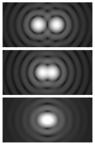
You’ll raise a third objection now: the radius of a proton is measured using the femtometer scale, so that’s expressed in 10−15 m, which is not 60 but a million times smaller than the nanometer (i.e. 10−9 m) scale used to express the Bohr radius as calculated by Feynman above. You’re right, but the 10−15 m number is the charge radius, not the uncertainty in position. Indeed, the so-called classical electron radius is also measured in femtometer and, hence, the Bohr radius is also like a million times that number. OK. That should settle the matter. I need to move on.

Before I do move on, let me relate the observation (i.e. the fact that the uncertainty in regard to position decreases as the mass of a particle increases) to another phenomenon. As you know, the interference of light beams is easy to observe. Hence, the interference of photons is easy to observe: Young’s experiment involved a slit of 0.85 mm (so almost 1 mm) only. In contrast, the 2012 double-slit experiment with electrons involved slits that were 62 nanometer wide, i.e. 62 billionths of a meter! That’s because the associated frequencies are so much higher and, hence, the wave zone is much smaller. So much, in fact, that Feynman could not imagine technology would ever be sufficiently advanced so as to actually carry out the double slit experiment with electrons. It’s an aspect of the same: the uncertainty in position is much smaller for electrons than it is for photons. Who knows: perhaps one day, we’ll be able to do the experiment with protons. 🙂 For further detail, I’ll refer you one of my posts on this.

What’s Explained, and What’s Left Unexplained?

There is another obvious question: if the electron is still some point charge, and going around as it does, why doesn’t it radiate energy? Indeed, the Rutherford-Bohr model had to be discarded because this ‘planetary’ model involved circular (or elliptical) motion and, therefore, some acceleration. According to classical theory, the electron should thus emit electromagnetic radiation, as a result of which it would radiate its kinetic energy away and, therefore, spiral in toward the nucleus. The quantum-mechanical model doesn’t explain this either, does it?

I can’t answer this question as yet, as I still need to go through all Feynman’s Lectures on quantum mechanics. You’re right. There’s something odd about the quantum-mechanical idea: it still involves a electron moving in some kind of orbital − although I hasten to add that the wavefunction is a complex-valued function, not some real function − but it does not involve any loss of kinetic energy due to circular motion apparently!

There are other unexplained questions as well. For example, the idea of an electrical point charge still needs to be re-conciliated with the mathematical inconsistencies it implies, as Feynman points out himself in yet another of his Lectures. :-/

Finally, you’ll wonder as to the difference between a proton and a positron: if a positron and an electron annihilate each other in a flash, why do we have a hydrogen atom at all? Well… The proton is not the electron’s anti-particle. For starters, it’s made of quarks, while the positron is made of… Well… A positron is a positron: it’s elementary. But, yes, interesting question, and the ‘mechanics’ behind the mutual destruction are quite interesting and, hence, surely worth looking into—but not here. 🙂

Having mentioned a few things that remain unexplained, the model does have the advantage of solving plenty of other questions. It explains, for example, why the electron and the proton are actually right on top of each other, as they should be according to classical electrostatic theory, and why they are not at the same time: the electron is still a sort of ‘cloud’ indeed, with the proton at its center.

The quantum-mechanical ‘cloud’ model of the electron also explains why “the terrific electrical forces balance themselves out, almost perfectly, by forming tight, fine mixtures of the positive and the negative, so there is almost no attraction or repulsion at all between two separate bunches of such mixtures” (Richard Feynman, Introduction to Electromagnetism, p. 1-1) or, to quote from one of his other writings, why we do not fall through the floor as we walk:

“As we walk, our shoes with their masses of atoms push against the floor with its mass of atoms. In order to squash the atoms closer together, the electrons would be confined to a smaller space and, by the uncertainty principle, their momenta would have to be higher on the average, and that means high energy; the resistance to atomic compression is a quantum-mechanical effect and not a classical effect. Classically, we would expect that if we were to draw all the electrons and protons closer together, the energy would be reduced still further, and the best arrangement of positive and negative charges in classical physics is all on top of each other. This was well known in classical physics and was a puzzle because of the existence of the atom. Of course, the early scientists invented some ways out of the trouble—but never mind, we have the right way out, now!”

So that’s it, then. Except… Well…

The Fine-Structure Constant

When talking about the stability of atoms, one cannot escape a short discussion of the so-called fine-structure constant, denoted by α (alpha). I discussed it another post of mine, so I’ll refer you there for a more comprehensive overview. I’ll just remind you of the basics:

(1) α is the square of the electron charge expressed in Planck units: α = eP2.

(2) α is the square root of the ratio of (a) the classical electron radius and (b) the Bohr radius: α = √(re /r). You’ll see this more often written as re = α2r. Also note that this is an equation that does not depend on the units, in contrast to equation 1 (above), and 4 and 5 (below), which require you to switch to Planck units. It’s the square of a ratio and, hence, the units don’t matter. They fall away.

(3) α is the (relative) speed of an electron: α = v/c. [The relative speed is the speed as measured against the speed of light. Note that the ‘natural’ unit of speed in the Planck system of units is equal to c. Indeed, if you divide one Planck length by one Planck time unit, you get (1.616×10⁻³⁵ m)/(5.391×10−44 s) = c m/s. However, this is another equation, just like (2), that does not depend on the units: we can express v and c in whatever unit we want, as long we’re consistent and express both in the same units.]

(4) Finally, α is also equal to the product of (a) the electron mass (which I’ll simply write as me here) and (b) the classical electron radius re (if both are expressed in Planck units): α = me·re. [I think that’s, perhaps, the most amazing of all of the expressions for α. If you don’t think that’s amazing, I’d really suggest you stop trying to study physics.]

Note that, from (2) and (4), we also find that:

(5) The electron mass (in Planck units) is equal me = α/re = α/α2r = 1/αr. So that gives us an expression, using α once again, for the electron mass as a function of the Bohr radius r expressed in Planck units.

Finally, we can also substitute (1) in (5) to get:

(6) The electron mass (in Planck units) is equal to me = α/re  = eP2/re. Using the Bohr radius, we get me = 1/αr = 1/eP2r.

In addition, in the mentioned post, I also related α to the so-called coupling constant determining the strength of the interaction between electrons and photons. So… What a magical number indeed ! It suggests some unity that our little model of the atom above doesn’t quite capture. As far as I am concerned, it’s one of the many other ‘unexplained questions’, and one of my key objectives, as I struggle through Feynman’s Lectures, is to understand it all. 🙂 One of the issues is, of course, how to relate this coupling constant to the concept of a gauge, which I briefly discussed in my previous post. In short, I’ve still got a long way to go… 😦

Post Scriptum: The de Broglie relations and the Uncertainty Principle

My little exposé on mass being nothing but a scale factor in the Uncertainty Principle is a good occasion to reflect on the Uncertainty Principle once more. Indeed, what’s the uncertainty about, if it’s not about the mass? It’s about the position in space and velocity, i.e. it’s movement and time. Velocity or speed (i.e. the magnitude of the velocity vector) is, in turn, defined as the distance traveled divided by the time of travel, so the uncertainty is about time as well, as evidenced from the ΔEΔt = h expression of the Uncertainty Principle. But how does it work exactly?

Hmm… Not sure. Let me try to remember the context. We know that the de Broglie relation, λ = h/p, which associates a wavelength (λ) with the momentum (p) of a particle, is somewhat misleading, because we’re actually associating a (possibly infinite) bunch of component waves with a particle. So we’re talking some range of wavelengths (Δλ) and, hence, assuming all these component waves travel at the same speed, we’re also talking a frequency range (Δf). The bottom line is that we’ve got a wave packet and we need to distinguish the velocity of its phase (vp) versus the group velocity (vg), which corresponds to the classical velocity of our particle.

I think I explained that pretty well in one of my previous posts on the Uncertainty Principle, so I’d suggest you have a look there. The mentioned post explains how the Uncertainty Principle relates position (x) and momentum (p) as a Fourier pair, and it also explains that general mathematical property of Fourier pairs: the more ‘concentrated’ one distribution is, the more ‘spread out’ its Fourier transform will be. In other words, it is not possible to arbitrarily ‘concentrate’ both distributions, i.e. both the distribution of x (which I denoted as Ψ(x) as well as its Fourier transform, i.e. the distribution of p (which I denoted by Φ(p)). So, if we’d ‘squeeze’ Ψ(x), then its Fourier transform Φ(p) will ‘stretch out’.

That was clear enough—I hope! But how do we go from ΔxΔp = h to ΔEΔt = h? Why are energy and time another Fourier pair? To answer that question, we need to clearly define what energy and what time we are talking about. The argument revolves around the second de Broglie relation: E = h·f. How do we go from the momentum p to the energy E? And how do we go from the wavelength λ to the frequency f?

The answer to the first question is the energy-mass equivalence: E = mc2, always. This formula is relativistic, as m is the relativistic mass, so it includes the rest mass m0 as well as the equivalent mass of its kinetic energy m0v2/2 + … [Note, indeed, that the kinetic energy – defined as the excess energy over its rest energy – is a rapidly converging series of terms, so only the m0v2/2 term is mentioned.] Likewise, momentum is defined as p = mv, always, with m the relativistic mass, i.e. m = (1−v2/c2)−1/2·m0 = γ·m0, with γ the Lorentz factor. The E = mc2 and p = mv relations combined give us the E/c = m·c = p·c/v or E·v/c = p·c relationship, which we can also write as E/p = c2/v. However, we’ll need to write E as a function of p for the purpose of a derivation. You can verify that E2 − p2c2 = m02c4) and, hence, that E = (p2c2 + m02c4)1/2.

Now, to go from a wavelength to a frequency, we need the wave velocity, and we’re obviously talking the phase velocity here, so we write: vp = λ·f. That’s where the de Broglie hypothesis comes in: de Broglie just assumed the Planck-Einstein relation E = h·ν, in which ν is the frequency of a massless photon, would also be valid for massive particles, so he wrote: E = h·f. It’s just a hypothesis, of course, but it makes everything come out alright. More in particular, the phase velocity vp = λ·f can now be re-written, using both de Broglie relations (i.e. h/p = λ and E/h = f) as vp = (E/h)·(p/h) = E/p = c2/v. Now, because v is always smaller than c for massive particles (and usually very much smaller), we’re talking a superluminal phase velocity here! However, because it doesn’t carry any signal, it’s not inconsistent with relativity theory.

Now what about the group velocity? To calculate the group velocity, we need the frequencies and wavelengths of the component waves. The dispersion relation assumes the frequency of each component wave can be expressed as a function of its wavelength, so f = f(λ). Now, it takes a bit of wave mechanics (which I won’t elaborate on here) to show that the group velocity is the derivative of f with respect to λ, so we write vg = ∂f/∂λ. Using the two de Broglie relations, we get: vg = ∂f/∂λ = ∂(E/h)/∂(p/h) = ∂E/∂p = ∂[p2c2 + m02c4)1/2]/∂p. Now, when you write it all out, you should find that vg = ∂f/∂λ = pc2/E = c2/vp = v, so that’s the classical velocity of our particle once again.

Phew! Complicated! Yes. But so we still don’t have our ΔEΔt = h expression! All of the above tells us how we can associate a range of momenta (Δp) with a range of wavelengths (Δλ) and, in turn, with a frequency range (Δf) which then gives us some energy range (ΔE), so the logic is like:

Δp ⇒ Δλ ⇒ Δf ⇒ ΔE

Somehow, the same sequence must also ‘transform’ our Δx into Δt. I googled a bit, but I couldn’t find any clear explanation. Feynman doesn’t seem to have one in his Lectures either so, frankly, I gave up. What I did do in one of my previous posts, is to give some interpretation. However, I am not quite sure if it’s really the interpretation: there are probably several ones. It must have something to do with the period of a wave, but I’ll let you break your head over it. 🙂 As far as I am concerned, it’s just one of the other unexplained questions I have as I sort of close my study of ‘classical’ physics. So I’ll just make a mental note of it. [Of course, please don’t hesitate to send me your answer, if you’d have one!] Now it’s time to really dig into quantum mechanics, so I should really stay silent for quite a while now! 🙂

Some content on this page was disabled on June 16, 2020 as a result of a DMCA takedown notice from The California Institute of Technology. You can learn more about the DMCA here:

https://wordpress.com/support/copyright-and-the-dmca/

The Uncertainty Principle revisited

Pre-script (dated 26 June 2020): This post has become less relevant (even irrelevant, perhaps) because my views on all things quantum-mechanical have evolved significantly as a result of my progression towards a more complete realist (classical) interpretation of quantum physics. I keep blog posts like these mainly because I want to keep track of where I came from. I might review them one day, but I currently don’t have the time or energy for it. 🙂

Original post:

I’ve written a few posts on the Uncertainty Principle already. See, for example, my post on the energy-time expression for it (ΔE·Δt ≥ h). So why am I coming back to it once more? Not sure. I felt I left some stuff out. So I am writing this post to just complement what I wrote before. I’ll do so by explaining, and commenting on, the ‘semi-formal’ derivation of the so-called Kennard formulation of the Principle in the Wikipedia article on it.

The Kennard inequalities, σxσp ≥ ħ/2 and σEσt ≥ ħ/2, are more accurate than the more general Δx·Δp ≥ h and ΔE·Δt ≥ h expressions one often sees, which are an early formulation of the Principle by Niels Bohr, and which Heisenberg himself used when explaining the Principle in a thought experiment picturing a gamma-ray microscope. I presented Heisenberg’s thought experiment in another post, and so I won’t repeat myself here. I just want to mention that it ‘proves’ the Uncertainty Principle using the Planck-Einstein relations for the energy and momentum of a photon:

E = hf and p = h/λ

Heisenberg’s thought experiment is not a real proof, of course. But then what’s a real proof? The mentioned ‘semi-formal’ derivation looks more impressive, because more mathematical, but it’s not a ‘proof’ either (I hope you’ll understand why I am saying that after reading my post). The main difference between Heisenberg’s thought experiment and the mathematical derivation in the mentioned Wikipedia article is that the ‘mathematical’ approach is based on the de Broglie relation. That de Broglie relation looks the same as the Planck-Einstein relation (p = h/λ) but it’s fundamentally different.

Indeed, the momentum of a photon (i.e. the p we use in the Planck-Einstein relation) is not the momentum one associates with a proper particle, such as an electron or a proton, for example (so that’s the p we use in the de Broglie relation). The momentum of a particle is defined as the product of its mass (m) and velocity (v). Photons don’t have a (rest) mass, and their velocity is absolute (c), so how do we define momentum for a photon? There are a couple of ways to go about it, but the two most obvious ones are probably the following:

  1. We can use the classical theory of electromagnetic radiation and show that the momentum of a photon is related to the magnetic field (we usually only analyze the electric field), and the so-called radiation pressure that results from it. It yields the p = E/c formula which we need to go from E = hf to p = h/λ, using the ubiquitous relation between the frequency, the wavelength and the wave velocity (c = λf). In case you’re interested in the detail, just click on the radiation pressure link).
  2. We can also use the mass-energy equivalence E = mc2. Hence, the equivalent mass of the photon is E/c2, which is relativistic mass only. However, we can multiply that mass with the photon’s velocity, which is c, thereby getting the very same value for its momentum p = c·E/c2 = E/c.

So Heisenberg’s ‘proof’ uses the Planck-Einstein relations, as it analyzes the Uncertainty Principle more as an observer effect: probing matter with light, so to say. In contrast, the mentioned derivation takes the de Broglie relation itself as the point of departure. As mentioned, the de Broglie relations look exactly the same as the Planck-Einstein relationship (E = hf and p = h/λ) but the model behind is very different. In fact, that’s what the Uncertainty Principle is all about: it says that the de Broglie frequency and/or wavelength cannot be determined exactly: if we want to localize a particle, somewhat at least, we’ll be dealing with a frequency range Δf. As such, the de Broglie relation is actually somewhat misleading at first. Let’s talk about the model behind.

A particle, like an electron or a proton, traveling through space, is described by a complex-valued wavefunction, usually denoted by the Greek letter psi (Ψ) or phi (Φ). This wavefunction has a phase, usually denoted as θ (theta) which – because we assume the wavefunction is a nice periodic function – varies as a function of time and space. To be precise, we write θ as θ = ωt – kx or, if the wave is traveling in the other direction, as θ = kx – ωt.

I’ve explained this in a couple of posts already, including my previous post, so I won’t repeat myself here. Let me just note that ω is the angular frequency, which we express in radians per second, rather than cycles per second, so ω = 2πf (one cycle covers 2π rad). As for k, that’s the wavenumber, which is often described as the spatial frequency, because it’s expressed in cycles per meter or, more often (and surely in this case), in radians per meter. Hence, if we freeze time, this number is the rate of change of the phase in space. Because one cycle is, again, 2π rad, and one cycle corresponds to the wave traveling one wavelength (i.e. λ meter), it’s easy to see that k = 2π/λ. We can use these definitions to re-write the de Broglie relations E = hf and p = h/λ as:

E = ħω and p = ħk with h = h/2π

What about the wave velocity? For a photon, we have c = λf and, hence, c = (2π/k)(ω/2π) = ω/k. For ‘particle waves’ (or matter waves, if you prefer that term), it’s much more complicated, because we need to distinguish between the so-called phase velocity (vp) and the group velocity (vg). The phase velocity is what we’re used to: it’s the product of the frequency (the number of cycles per second) and the wavelength (the distance traveled by the wave over one cycle), or the ratio of the angular frequency and the wavenumber, so we have, once again, λf = ω/k = vp. However, this phase velocity is not the classical velocity of the particle that we are looking at. That’s the so-called group velocity, which corresponds to the velocity of the wave packet representing the particle (or ‘wavicle’, if your prefer that term), as illustrated below.

Wave_packet_(dispersion)

The animation below illustrates the difference between the phase and the group velocity even more clearly: the green dot travels with the ‘wavicles’, while the red dot travels with the phase. As mentioned above, the group velocity corresponds to the classical velocity of the particle (v). However, the phase velocity is a mathematical point that actually travels faster than light. It is a mathematical point only, which does not carry a signal (unlike the modulation of the wave itself, i.e. the traveling ‘groups’) and, hence, it does not contradict the fundamental principle of relativity theory: the speed of light is absolute, and nothing travels faster than light (except mathematical points, as you can, hopefully, appreciate now).

Wave_group (1)

The two animations above do not represent the quantum-mechanical wavefunction, because the functions that are shown are real-valued, not complex-valued. To imagine a complex-valued wave, you should think of something like the ‘wavicle’ below or, if you prefer animations, the standing waves underneath (i.e. C to H: A and B just present the mathematical model behind, which is that of a mechanical oscillator, like a mass on a spring indeed). These representations clearly show the real as well as the imaginary part of complex-valued wave-functions.

Photon wave

QuantumHarmonicOscillatorAnimation

With this general introduction, we are now ready for the more formal treatment that follows. So our wavefunction Ψ is a complex-valued function in space and time. A very general shape for it is one we used in a couple of posts already:

Ψ(x, t) ∝ ei(kx – ωt) = cos(kx – ωt) + isin(kx – ωt)

If you don’t know anything about complex numbers, I’d suggest you read my short crash course on it in the essentials page of this blog, because I don’t have the space nor the time to repeat all of that. Now, we can use the de Broglie relationship relating the momentum of a particle with a wavenumber (p = ħk) to re-write our psi function as:

Ψ(x, t) ∝ ei(kx – ωt) = ei(px/ħ – ωt) 

Note that I am using the ‘proportional to’ symbol (∝) because I don’t worry about normalization right now. Indeed, from all of my other posts on this topic, you know that we have to take the absolute square of all these probability amplitudes to arrive at a probability density function, describing the probability of the particle effectively being at point x in space at point t in time, and that all those probabilities, over the function’s domain, have to add up to 1. So we should insert some normalization factor.

Having said that, the problem with the wavefunction above is not normalization really, but the fact that it yields a uniform probability density function. In other words, the particle position is extremely uncertain in the sense that it could be anywhere. Let’s calculate it using a little trick: the absolute square of a complex number equals the product of itself with its (complex) conjugate. Hence, if z = reiθ, then │z│2 = zz* = reiθ·re–iθ = r2eiθ–iθ = r2e0 = r2. Now, in this case, assuming unique values for k, ω, p, which we’ll note as k0, ω0, p0 (and, because we’re freezing time, we can also write t = t0), we should write:

│Ψ(x)│2 = │a0ei(p0x/ħ – ω0t0) │2 = │a0eip0x/ħ e–iω0t0 │2 = │a0eip0x/ħ │2 │e–iω0t0 │2 = a02 

Note that, this time around, I did insert some normalization constant a0 as well, so that’s OK. But so the problem is that this very general shape of the wavefunction gives us a constant as the probability for the particle being somewhere between some point a and another point b in space. More formally, we get the surface for a rectangle when we calculate the probability P[a ≤ X ≤ b] as we should calculate it, which is as follows:

integral

More specifically, because we’re talking one-dimensional space here, we get P[a ≤ X ≤ b] = (b–a)·a02. Now, you may think that such uniform probability makes sense. For example, an electron may be in some orbital around a nucleus, and so you may think that all ‘points’ on the orbital (or within the ‘sphere’, or whatever volume it is) may be equally likely. Or, in another example, we may know an electron is going through some slit and, hence, we may think that all points in that slit should be equally likely positions. However, we know that it is not the case. Measurements show that not all points are equally likely. For an orbital, we get complicated patterns, such as the one shown below, and please note that the different colors represent different complex numbers and, hence, different probabilities.

Hydrogen_eigenstate_n5_l2_m1

Also, we know that electrons going through a slit will produce an interference pattern—even if they go through it one by one! Hence, we cannot associate some flat line with them: it has to be a proper wavefunction which implies, once again, that we can’t accept a uniform distribution.

In short, uniform probability density functions are not what we see in Nature. They’re non-uniform, like the (very simple) non-uniform distributions shown below. [The left-hand side shows the wavefunction, while the right-hand side shows the associated probability density function: the first two are static (i.e. they do not vary in time), while the third one shows a probability distribution that does vary with time.]

StationaryStatesAnimation

I should also note that, even if you would dare to think that a uniform distribution might be acceptable in some cases (which, let me emphasize this, it is not), an electron can surely not be ‘anywhere’. Indeed, the normalization condition implies that, if we’d have a uniform distribution and if we’d consider all of space, i.e. if we let a go to –∞ and b to +∞, then a02 would tend to zero, which means we’d have a particle that is, literally, everywhere and nowhere at the same time.

In short, a uniform probability distribution does not make sense: we’ll generally have some idea of where the particle is most likely to be, within some range at least. I hope I made myself clear here.

Now, before I continue, I should make some other point as well. You know that the Planck constant (h or ħ) is unimaginably small: about 1×10⁻³⁴ J·s (joule-second). In fact, I’ve repeatedly made that point in various posts. However, having said that, I should add that, while it’s unimaginably small, the uncertainties involved are quite significant. Let us indeed look at the value of ħ by relating it to that σxσp ≥ ħ/2 relation.

Let’s first look at the units. The uncertainty in the position should obviously be expressed in distance units, while momentum is expressed in kg·m/s units. So that works out, because 1 joule is the energy transferred (or work done) when applying a force of 1 newton (N) over a distance of 1 meter (m). In turn, one newton is the force needed to accelerate a mass of one kg at the rate of 1 meter per second per second (this is not a typing mistake: it’s an acceleration of 1 m/s per second, so the unit is m/s2: meter per second squared). Hence, 1 J·s = 1 N·m·s = 1 kg·m/s2·m·s = kg·m2/s. Now, that’s the same dimension as the ‘dimensional product’ for momentum and distance: m·kg·m/s = kg·m2/s.

Now, these units (kg, m and s) are all rather astronomical at the atomic scale and, hence, h and ħ are usually expressed in other dimensions, notably eV·s (electronvolt-second). However, using the standard SI units gives us a better idea of what we’re talking about. If we split the ħ = 1×10⁻³⁴ J·s value (let’s forget about the 1/2 factor for now) ‘evenly’ over σx and σp – whatever that means: all depends on the units, of course!  – then both factors will have magnitudes of the order of 1×10⁻¹⁷: 1×10−17 m times 1×10−17 kg·m/s gives us 1×10⁻³⁴ J·s.

You may wonder how this 1×10⁻¹⁷ m compares to, let’s say, the classical electron radius, for example. The classical electron radius is, roughly speaking, the ‘space’ an electron seems to occupy as it scatters incoming light. The idea is illustrated below (credit for the image goes to Wikipedia, as usual). The classical electron radius – or Thompson scattering length – is about 2.818×10⁻¹⁵ m, so that’s almost 300 times our ‘uncertainty’ (1×10⁻¹⁷ m). Not bad: it means that we can effectively relate our ‘uncertainty’ in regard to the position to some actual dimension in space. In this case, we’re talking the femtometer scale (1 fm = 10−15 m), and so you’ve surely heard of this before.

Thomson_scattering_geometry

What about the other ‘uncertainty’, the one for the momentum (1×10⁻¹⁷ kg·m/s)? What’s the typical (linear) momentum of an electron? Its mass, expressed in kg, is about 9.1×10⁻³¹ kg. We also know its relative velocity in an electron: it’s that magical number α = v/c, about which I wrote in some other posts already, so v = αc ≈ 0.0073·3×108 m/s ≈ 2.2×10⁶ m/s. Now, 9.1×10−31 kg times 2.2×106 m/s is about 2×10–26 kg·m/s, so our proposed ‘uncertainty’ in regard to the momentum (1×10⁻¹⁷ kg·m/s) is half a billion times larger than the typical value for it. Now that is, obviously, not so good. [Note that calculations like this are extremely rough. In fact, when one talks electron momentum, it’s usual angular momentum, which is ‘analogous’ to linear momentum, but angular momentum involves very different formulas. If you want to know more about this, check my post on it.]

Of course, now you may feel that we didn’t ‘split’ the uncertainty in a way that makes sense: those –17 exponents don’t work, obviously. So let’s take 1×10–26 kg·m/s for σp, which is half of that ‘typical’ value we calculated. Then we’d have 1×10⁻⁸ m for σx (1×10−8 m times 1×10–26 kg·m/s is, once again, 1×10–34 J·s). But then that uncertainty suddenly becomes a huge number: 1×10⁻⁸ m is 100 angstrom. That’s not the atomic scale but the molecular scale! So it’s huge as compared to the pico- or femto-meter scale (1 pm = 1×10⁻¹² m, 1 fm = 1×10⁻¹⁵ m) which we’d sort of expect to see when we’re talking electrons.

OK. Let me get back to the lesson. Why this digression? Not sure. I think I just wanted to show that the Uncertainty Principle involves ‘uncertainties’ that are extremely relevant: despite the unimaginable smallness of the Planck constant, these uncertainties are quite significant at the atomic scale. But back to the ‘proof’ of Kennard’s formulation. Here we need to discuss the ‘model’ we’re using. The rather simple animation below (again, credit for it has to go to Wikipedia) illustrates it wonderfully.

Sequential_superposition_of_plane_waves

Look at it carefully: we start with a ‘wave packet’ that looks a bit like a normal distribution, but it isn’t, of course. We have negative and positive values, and normal distributions don’t have that. So it’s a wave alright. Of course, you should, once more, remember that we’re only seeing one part of the complex-valued wave here (the real or imaginary part—it could be either). But so then we’re superimposing waves on it. Note the increasing frequency of these waves, and also note how the wave packet becomes increasingly localized with the addition of these waves. In fact, the so-called Fourier analysis, of which you’ve surely heard before, is a mathematical operation that does the reverse: it separates a wave packet into its individual component waves.

So now we know the ‘trick’ for reducing the uncertainty in regard to the position: we just add waves with different frequencies. Of course, different frequencies imply different wavenumbers and, through the de Broglie relationship, we’ll also have different values for the ‘momentum’ associated with these component waves. Let’s write these various values as kn, ωn, and pn respectively, with n going from 0 to N. Of course, our point in time remains frozen at t0. So we get a wavefunction that’s, quite simply, the sum of N component waves and so we write:

Ψ(x) = ∑ anei(pnx/ħ – ωnt0) = ∑ an  eipnx/ħe–iωnt0 = ∑ Aneipnx/ħ

Note that, because of the e–iωnt0, we now have complex-valued coefficients An = ane–iωnt0 in front. More formally, we say that An represents the relative contribution of the mode pn to the overall Ψ(x) wave. Hence, we can write these coefficients A as a function of p. Because Greek letters always make more of an impression, we’ll use the Greek letter Φ (phi) for it. 🙂 Now, we can go to the continuum limit and, hence, transform that sum above into an infinite sum, i.e. an integral. So our wave function then becomes an integral over all possible modes, which we write as:

wave function integral

Don’t worry about that new 1/√2πħ factor in front. That’s, once again, something that has to do with normalization and scales. It’s the integral itself you need to understand. We’ve got that Φ(p) function there, which is nothing but our An coefficient, but for the continuum case. In fact, these relative contributions Φ(p) are now referred to as the amplitude of all modes p, and so Φ(p) is actually another wave function: it’s the wave function in the so-called momentum space.

You’ll probably be very confused now, and wonder where I want to go with an integral like this. The point to note is simple: if we have that Φ(p) function, we can calculate (or derive, if you prefer that word) the Ψ(x) from it using that integral above. Indeed, the integral above is referred to as the Fourier transform, and it’s obviously closely related to that Fourier analysis we introduced above.

Of course, there is also an inverse transform, which looks exactly the same: it just switches the wave functions (Ψ and Φ) and variables (x and p), and then (it’s an important detail!), it has a minus sign in the exponent. Together, the two functions –  as defined by each other through these two integrals – form a so-called Fourier integral pair, also known as a Fourier transform pair, and the variables involved are referred to as conjugate variables. So momentum (p) and position (x) are conjugate variables and, likewise, energy and time are also conjugate variables (but so I won’t expand on the time-energy relation here: please have a look at one of my others posts on that).

Now, I thought of copying and explaining the proof of Kennard’s inequality from Wikipedia’s article on the Uncertainty Principle (you need to click on the show button in the relevant section to see it), but then that’s pretty boring math, and simply copying stuff is not my objective with this blog. More importantly, the proof has nothing to do with physics. Nothing at all. Indeed, it just proves a general mathematical property of Fourier pairs. More specifically, it proves that, the more concentrated one function is, the more spread out its Fourier transform must be. In other words, it is not possible to arbitrarily concentrate both a function and its Fourier transform.

So, in this case, if we’d ‘squeeze’ Ψ(x), then its Fourier transform Φ(p) will ‘stretch out’, and so that’s what the proof in that Wikipedia article basically shows. In other words, there is some ‘trade-off’ between the ‘compaction’ of Ψ(x), on the one hand, and Φ(p), on the other, and so that is what the Uncertainty Principle is all about. Nothing more, nothing less.

But… Yes? What’s all this talk about ‘squeezing’ and ‘compaction’? We can’t change reality, can we? Well… Here we’re entering the philosophical field, of course. How do we interpret the Uncertainty Principle? It surely does look like us trying to measure something has some impact on the wavefunction. In fact, usually, our measurement – of either position or momentum – usually makes the wavefunctions collapse: we suddenly know where the particle is and, hence, ψ(x) seems to collapse into one point. Alternatively, we measure its momentum and, hence, Φ(p) collapses.

That’s intriguing. In fact, even more intriguing is the possibility we may only partially affect those wavefunctions with measurements that are somewhat less ‘drastic’. It seems a lot of research is focused on that (just Google for partial collapse of the wavefunction, and you’ll finds tons of references, including presentations like this one).

Hmm… I need to further study the topic. The decomposition of a wave into its component waves is obviously something that works well in physics—and not only in quantum mechanics but also in much more mundane examples. Its most general application is signal processing, in which we decompose a signal (which is a function of time) into the frequencies that make it up. Hence, our wavefunction model makes a lot of sense, as it mirrors the physics involved in oscillators and harmonics obviously.

Still… I feel it doesn’t answer the fundamental question: what is our electron really? What do those wave packets represent? Physicists will say questions like this don’t matter: as long as our mathematical models ‘work’, it’s fine. In fact, if even Feynman said that nobody – including himself – truly understands quantum mechanics, then I should just be happy and move on. However, for some reason, I can’t quite accept that. I should probably focus some more on that de Broglie relationship, p = h/λ, as it’s obviously as fundamental to my understanding of the ‘model’ of reality in physics as that Fourier analysis of the wave packet. So I need to do some more thinking on that.

The de Broglie relationship is not intuitive. In fact, I am not ashamed to admit that it actually took me quite some time to understand why we can’t just re-write the de Broglie relationship (λ = h/p) as an uncertainty relation itself: Δλ = h/Δp. Hence, let me be very clear on this:

Δx = h/Δp (that’s the Uncertainty Principle) but Δλ ≠ h/Δp !

Let me quickly explain why.

If the Δ symbol expresses a standard deviation (or some other measurement of uncertainty), we can write the following:

p = h/λ ⇒ Δp = Δ(h/λ) = hΔ(1/λ) ≠ h/Δp

So I can take h out of the brackets after the Δ symbol, because that’s one of the things that’s allowed when working with standard deviations. More in particular, one can prove the following:

  1. The standard deviation of some constant function is 0: Δ(k) = 0
  2. The standard deviation is invariant under changes of location: Δ(x + k) = Δ(x + k)
  3. Finally, the standard deviation scales directly with the scale of the variable: Δ(kx) = |k |Δ(x).

However, it is not the case that Δ(1/x) = 1/Δx. However, let’s not focus on what we cannot do with Δx: let’s see what we can do with it. Δx equals h/Δp according to the Uncertainty Principle—if we take it as an equality, rather than as an inequality, that is. And then we have the de Broglie relationship: p = h/λ. Hence, Δx must equal:

Δx = h/Δp = h/[Δ(h/λ)] =h/[hΔ(1/λ)] = 1/Δ(1/λ)

That’s obvious, but so what? As mentioned, we cannot write Δx = Δλ, because there’s no rule that says that Δ(1/λ) = 1/Δλ and, therefore, h/Δp ≠ Δλ. However, what we can do is define Δλ as an interval, or a length, defined by the difference between its lower and upper bound (let’s denote those two values by λa and λb respectively. Hence, we write Δλ = λb – λa. Note that this does not assume we have a continuous range of values for λ: we can have any number of frequencies λn between λa and λb, but so you see the point: we’ve got a range of values λ, discrete or continuous, defined by some lower and upper bound.

Now, the de Broglie relation associates two values pa and pb with λa and λb respectively:  pa = h/λa and pb = h/λb. Hence, we can similarly define the corresponding Δp interval as pa – pb, with pa = h/λa and pb = h/λb. Note that, because we’re taking the reciprocal, we have to reverse the order of the values here: if λb > λa, then pa = h/λa > pb = h/λb. Hence, we can write Δp = Δ(h/λ) = pa – pb = h/λ1 – h/λ2 = h(1/λ1 – 1/λ2) = h[λ2 – λ1]/λ1λ2. In case you have a bit of difficulty, just draw some reciprocal functions (like the ones below), and have fun connecting intervals on the horizontal axis with intervals on the vertical axis using these functions.

graph

Now, h[λ2 – λ1]/λ1λ2) is obviously something very different than h/Δλ = h/(λ2 – λ1). So we can surely not equate the two and, hence, we cannot write that Δp = h/Δλ.

Having said that, the Δx = 1/Δ(1/λ) = λ1λ2/(λ2 – λ1) that emerges here is quite interesting. We’ve got a ratio here, λ1λ2/(λ2 – λ1, which shows that Δx depends only on the upper and lower bounds of the Δλ range. It does not depend on whether or not the interval is discrete or continuous.

The second thing that is interesting to note is Δx depends not only on the difference between those two values (i.e. the length of the interval) but also on their value: if the length of the interval, i.e. the difference between the two frequencies is the same, but their values as such are higher, then we get a higher value for Δx, i.e. a greater uncertainty in the position. Again, this shows that the relation between Δλ and Δx is not straightforward. But so we knew that already, and so I’ll end this post right here and right now. 🙂    

Some content on this page was disabled on June 17, 2020 as a result of a DMCA takedown notice from Michael A. Gottlieb, Rudolf Pfeiffer, and The California Institute of Technology. You can learn more about the DMCA here:

https://wordpress.com/support/copyright-and-the-dmca/

The wave-particle duality revisited

Pre-script (dated 26 June 2020): This post has become less relevant (even irrelevant, perhaps) because my views on all things quantum-mechanical have evolved significantly as a result of my progression towards a more complete realist (classical) interpretation of quantum physics. I keep blog posts like these mainly because I want to keep track of where I came from. I might review them one day, but I currently don’t have the time or energy for it. 🙂

Original post:

As an economist, having some knowledge of what’s around in my field (social science), I think I am well-placed to say that physics is not an easy science. Its ‘first principles’ are complicated, and I am not ashamed to say that, after more than a year of study now, I haven’t reached what I would call a ‘true understanding’ of it.

Sometimes, the teachers are to be blamed. For example, I just found out that, in regard to the question of the wave function of a photon, the answer of two nuclear scientists was plain wrong. Photons do have a de Broglie wave, and there is a fair amount of research and actual experimenting going on trying to measure it. One scientific article which I liked in particular, and I hope to fully understand a year from now or so, is on such ‘direct measurement of the (quantum) wavefunction‘. For me, it drove home the message that these idealized ‘thought experiments’ that are supposed to make autodidacts like me understand things better, are surely instructive in regard to the key point, but confusing in other respects.

A typical example of such idealized thought experiment is the double-slit experiment with ‘special detectors’ near the slits, which may or may not detect a photon, depending on whether or not they’re switched on as well as on their accuracy. Depending on whether or not the detectors are switched on, and their accuracy, we get full interference (a), no interference (b), or a mixture of (a) and (b), as shown in (c) and (d).

set-up photons double-slit photons - results

I took the illustrations from Feynman’s lovely little book, QED – The Strange Theory of Light and Matter, and he surely knows what he’s talking about. Having said that, the set-up raises a key question in regard to these detectors: how do they work, exactly? More importantly, how do they disturb the photons?

I googled for actual double-slit experiments with such ‘special detectors’ near the slits, but only found such experiments for electrons. One of these, a 2010 experiment of an Italian team, suggests that it’s the interaction between the detector and the electron wave that may cause the interference pattern to disappear. The idea is shown below. The electron is depicted as an incoming plane wave, which breaks up as it goes through the slits. The slit on the left has no ‘filter’ (which you may think of as a detector) and, hence, the plane wave goes through as a cylindrical wave. The slit on the right-hand side is covered by a ‘filter’ made of several layers of ‘low atomic number material’, so the electron goes through but, at the same time, the barrier creates a spherical wave as it goes through. The researchers note that “the spherical and cylindrical wave do not have any phase correlation, and so even if an electron passed through both slits, the two different waves that come out cannot create an interference pattern on the wall behind them.” [Needless to say, while being represented as ‘real’ waves here, the ‘waves’ are, in fact, complex-valued psi functions.]

double-slit experiment

In fact, to be precise, there actually still was an interference effect if the filter was thin enough. Let me quote the reason for that: “The thicker the filter, the greater the probability for inelastic scattering. When the electron suffers inelastic scattering, it is localized. This means that its wavefunction collapses and, after the measurement act, it propagates roughly as a spherical wave from the region of interaction, with no phase relation at all with other elastically or inelastically scattered electrons. If the filter is made thick enough, the interference effects cancels out almost completely.”

This, of course, doesn’t solve the mystery. The mystery, in such experiments, is that, when we put detectors, it is either the detector at A or the detector at B that goes off. They should never go off together—”at half strength, perhaps?”, as Feynman puts it. That’s why I used italics when writing “even if an electron passed through both slits.” The electron, or the photon in a similar set-up, is not supposed to do that. As mentioned above, the wavefunction collapses or reduces. Now that’s where these so-called ‘weak measurement’ experiments come in: they indicate the interaction doesn’t have to be that way. It’s not all or nothing: our observations should not necessarily destroy the wavefunction. So, who knows, perhaps we will be able, one day, to show that the wavefunction does go through both slits, as it should (otherwise the interference pattern cannot be explained), and then we will have resolved the paradox.

I am pretty sure that, when that’s done, physicists will also be able to relate the image of a photon as a transient electromagnetic wave (first diagram below), being emitted by an atomic oscillator for a few nanoseconds only (we gave the example for sodium light, for which the decay time was 3.2×10⁻⁸ seconds) with the image of a photon as a de Broglie wave (second diagram below). I look forward to that day. I think it will come soon.

Photon wavePhoton wave

Diffraction and the Uncertainty Principle (II)

Pre-script (dated 26 June 2020): This post did not suffer too much from the attack on this blog by the the dark force. It remains relevant. 🙂

Original post:

In my previous post, I derived and explained the general formula for the pattern generated by a light beam going through a slit or a circular aperture: the diffraction pattern. For light going through an aperture, this generates the so-called Airy pattern. In practice, diffraction causes a blurring of the image, and may make it difficult to distinguish two separate points, as shown below (credit for the image must go to Wikipedia again, I am afraid).

Airy_disk_spacing_near_Rayleigh_criterion

What’s actually going on is that the lens acts as a slit or, if it’s circular (which is usually the case), as an aperture indeed: the wavefront of the transmitted light is taken to be spherical or plane when it exits the lens and interferes with itself, thereby creating the ring-shaped diffraction pattern that we explained in the previous post.

The spatial resolution is also known as the angular resolution, which is quite appropriate, because it refers to an angle indeed: we know the first minimum (i.e. the first black ring) occurs at an angle θ such that sinθ = λ/L, with λ the wavelength of the light and L the lens diameter. It’s good to remind ourselves of the geometry of the situation: below we picture the array of oscillators, and so we know that the first minimum occurs at an angle such that Δ = λ. The second, third, fourth etc minimum occurs at an angle θ such that Δ = 2λ, 3λ, 4λ, etc. However, these secondary minima do not play any role in determining the resolving power of a lens, or a telescope, or an electron microscope, etc, and so you can just forget about them for the time being.

geometry

For small angles (expressed in radians), we can use the so-called small-angle approximation and equate sinθ with θ: the error of this approximation is less than one percent for angles smaller than 0.244 radians (14°), so we have the amazingly simply result that the first minimum occurs at an angle θ such that:

θ = λ/L

Spatial resolution of a microscope: the Rayleigh criterion versus Dawes’ limit 

If we have two point sources right next to each other, they will create two Airy disks, as shown above, which may overlap. That may make it difficult to see them, in a telescope, a microscope, or whatever device. Hence, telescopes, microscopes (using light or electron beams or whatever) have a limited resolving power. How do we measure that?

The so-called Rayleigh criterion regards two point sources as just resolved when the principal diffraction maximum of one image coincides with the first minimum of the other, as shown below. If the distance is greater, the two points are (very) well resolved, and if it is smaller, they are regarded as not resolved. This angle is obviously related to the θ = λ/L angle but it’s not the same: in fact, it’s a slightly wider angle. The analysis involved in calculating the angular resolution in terms of angle, and we use the same symbol θ for it, is quite complicated and so I’ll skip that and just give you the result:

θ = 1.22λ/L

two point sourcesRayleigh criterion

Note that, in this equation, θ stands for the angular resolution, λ for the wavelength of the light being used, and L is the diameter of the (aperture of) the lens. In the first of the three images above, the two points are well separated and, hence, the angle between them is well above the angular resolution. In the second, the angle between just meets the Rayleigh criterion, and in the third the angle between them is smaller than the angular resolution and, hence, the two points are not resolved.

Of course, the Rayleigh criterion is, to some extent, a matter of judgment. In fact, an English 19th century astronomer, named William Rutter Dawes, actually tested human observers on close binary stars of equal brightness, and found they could make out the two stars within an angle that was slightly narrower than the one given by the Rayleigh criterion. Hence, for an optical telescope, you’ll also find the simple θ = λ/L formula, so that’s the formula without the 1.22 factor (of course, λ here is, once again, the wavelength of the observed light or radiation, and L is the diameter of the telescope’s primary lens). This very simple formula allows us, for example, to calculate the diameter of the telescope lens we’d need to build to separate (see) objects in space with a resolution of, for example, 1 arcsec (i.e. 1/3600 of a degree or π/648,000 of a radian). Indeed, if we filter for yellow light only, which has a wavelength of 580 nm, we find L = 580×10−9 m/(π/648,000) = 0.119633×10⁻⁶ m ≈ 12 cm. [Just so you know: that’s about the size of the lens aperture of a good telescope (4 or 6 inches) for amateur astronomers–just in case you’d want one. :-)]

This simplified formula is called Dawes’ limit, and you’ll often see it used instead of Rayleigh’s criterion. However, the fact that it’s exactly the same formula as our formula for the first minimum of the Airy pattern should not confuse you: angular resolution is something different.

Now, after this introduction, let me get to the real topic of this post: Heisenberg’s Uncertainty Principle according to Heisenberg.

Heisenberg’s Uncertainty Principle according to Heisenberg

I don’t know about you but, as a kid, I didn’t know much about waves and fields and all that, and so I had difficulty understanding why the resolving power of a microscope or any other magnifying device depended on the frequency or wavelength. I now know my understanding was limited because I thought the concept of the amplitude of an electromagnetic wave had some spatial meaning, like the amplitude of a water or a sound wave. You know what I mean: this false idea that an electromagnetic wave is something that sort of wriggles through space, just like a water or sound wave wriggle through their medium (water and air respectively). Now I know better: the amplitude of an electromagnetic wave measures field strength and there’s no medium (no aether). So it’s not like a wave going around some object, or making some medium oscillate. I am not ashamed to acknowledge my stupidity at the time: I am just happy I finally got it, because it helps to really understand Heisenberg’s own illustration of his Uncertainty Principle, which I’ll present now.

Heisenberg imagined a gamma-ray microscope, as shown below (I copied this from the website of the American Institute for Physics ). Gamma-ray microscopes don’t exist – they’re hard to produce: you need a nuclear reactor or so 🙂 – but, as Heisenberg saw the development of new microscopes using higher and higher energy beams (as opposed to the 1.5-3 eV light in the visible spectrum) so as to increase the angular resolution and, hence, be able to see smaller things, he imagined one could use, perhaps, gamma-rays for imaging. Gamma rays are the hardest radiation, with frequencies of 10 exaherz and more (or >1019 Hz) and, hence, energies above 100 keV (i.e. 100,000 more than photons in the visible light spectrum, and 1000 times more than the electrons used in an average electron microscope). Gamma rays are not the result of some electron jumping from a higher to a lower energy level: they are emitted in decay processes of atomic nuclei (gamma decay). But I am digressing. Back to the main story line. So Heisenberg imagined we could ‘shine’ gamma rays on an electron and that we could then ‘see’ that electron in the microscope because some of the gamma photons would indeed end up in the microscope after their ‘collision’ with the electron, as shown below.

gammaray

The experiment is described in many places elsewhere but I found these accounts often confusing, and so I present my own here. 🙂

What Heisenberg basically meant to show is that this set-up would allow us to gather precise information on the position of the electron–because we would know where it was–but that, as a result, we’d lose information in regard to its momentum. Why? To put it simply: because the electron recoils as a result of the interaction. The point, of course, is to calculate the exact relationship between the two (position and momentum). In other words: what we want to do is to state the Uncertainty Principle quantitatively, not qualitatively.

Now, the animation above uses the symbol L for the γ-ray wavelength λ, which is confusing because I used L for the diameter of the aperture in my explanation of diffraction above. The animation above also uses a different symbol for the angular resolution: A instead of θ. So let me borrow the diagram used in the Wikipedia article and rephrase the whole situation.

Heisenberg_Microscope

From the diagram above, it’s obvious that, to be scattered into the microscope, the γ-ray photon must be scattered into a cone with angle ε. That angle is obviously related to the angular resolution of the microscope, which is θ = ε/2 = λ/D, with D the diameter of the aperture (i.e. the primary lens). Now, the electron could actually be anywhere, and the scattering angle could be much larger than ε, and, hence, relating D to the uncertainty in position (Δx) is not as obvious as most accounts of this thought experiment make it out to be. The thing is: if the scattering angle is larger than ε, it won’t reach the light detector at the end of the microscope (so that’s the flat top in the diagram above). So that’s why we can equate D with Δx, so we write Δx = ± D/2 = D. To put it differently: the assumption here is basically that this imaginary microscope ‘sees’ an area that is approximately as large as the lens. Using the small-angle approximation (so we write sin(2ε) ≈ 2ε), we can write:

Δx = 2λ/ε

Now, because of the recoil effect, the electron receives some momentum from the γ-ray photon. How much? Well… The situation is somewhat complicated (much more complicated than the Wikipedia article on this very same topic suggests), because the photon keeps some but also gives some of its original momentum. In fact, what’s happening really is Compton scattering: the electron first absorbs the photon, and then emits another with a different energy and, hence, also with different frequency and wavelength. However, what we do now is that the photon’s original momentum was equal to E/c= p = h/λ. That’s just the Planck relation or, if you’d want to look at the photon as a particle, the de Broglie equation.

Now, because we’re doing an analysis in one dimension only (x), we’re only going to look at the momentum in this direction only, i.e. px, and we’ll assume that all of the momentum of the photon before the interaction (or ‘collision’ if you want) was horizontal. Hence, we can write px = h/λ. After the collision, however, this momentum is spread over the electron and the scattered or emitted photon that’s going into the microscope. Let’s now imagine the two extremes:

  1. The scattered photon goes to the left edge of the lens. Hence, its horizontal momentum is negative (because it moves to the left) and the momentum px will be distributed over the electron and the photon such that px = p’x –h(ε/2)/λ’. Why the ε/2 factor? Well… That’s just trigonometry: the horizontal momentum of the scattered photon is obviously only a tiny fraction of its original horizontal momentum, and that fraction is given by the angle ε/2.
  2. The scattered photon goes to the right edge of the lens. In that case, we write px = p”x + h(ε/2)/λ”.

Now, the spread in the momentum of the electron, which we’ll simply write as Δp, is obviously equal to:

Δp = p”x – p’x = px + h(ε/2)/λ” – px + h(ε/2)/λ’ = h(ε/2)/λ” + h(ε/2)/λ’ = h(ε/2)/λ” + h(ε/2)/λ’

That’s a nice formula, but what can we do with it? What we want is a relationship between Δx and Δp, i.e. the position and the momentum of the electron, and of the electron only. That involves another simplification, which is also dealt with very summarily – too summarily in my view – in most accounts of this experiment. So let me spell it out. The angle ε is obviously very small and, hence, we may equate λ’ and λ”. In addition, while these two wavelengths differ from the wavelength of the incoming photon, the scattered photon is, obviously, still a gamma ray and, therefore, we are probably not too far off when substituting both λ’ and λ” for λ, i.e. the frequency of the incoming γ-ray. Now, we can re-write Δx = 2λ/ε as 1/Δx = ε/(2λ). We then get:

Δp = p”x – p’x = hε/2λ” + hε/2λ’ = 2hε/2λ = 2h/Δx

Now that yields ΔpΔx = 2h, which is an approximate expression of Heisenberg’s Uncertainty Principle indeed (don’t worry about the factor 2, as that’s something that comes with all of the approximations).

A final moot point perhaps: it is obviously a thought experiment. Not only because we don’t have gamma-ray microscopes (that’s not relevant because we can effectively imagine constructing one) but because the experiment involves only one photon. A real microscope would organize a proper beam, but that would obviously complicate the analysis. In fact, it would defeat the purpose, because the whole point is to analyze one single interaction here.

The interpretation

Now how should we interpret all of this? Is this Heisenberg’s ‘proof’ of his own Principle? Yes and no, I’d say. It’s part illustration, and part ‘proof’, I would say. The crucial assumptions here are:

  1. We can analyze γ-ray photons, or any photon for that matter, as particles having some momentum, and when ‘colliding’, or interacting, with an electron, the photon will impart some momentum to that electron.
  2. Momentum is being conserved and, hence, the total (linear) momentum before and after the collision, considering both particles–i.e. (1) the incoming ray and the electron before the interaction and (2) the emitted photon and the electron that’s getting the kick after the interaction–must be the same.
  3. For the γ-ray photon, we can relate (or associate, if you prefer that term) its wavelength λ with its momentum p through the Planck relation or, what amounts to the same for photons (because they have no mass), the de Broglie relation.

Now, these assumptions are then applied to an analysis of what we know to be true from experiment, and that’s the phenomenon of diffraction, part of which is the observation that the resolving power of a microscope is limited, and that its resolution is given by the θ = λ/D equation.

Bringing it all together, then gives us a theory which is consistent with experiment and, hence, we then assume the theory is true. Why? Well… I could start a long discourse here on the philosophy of science but, when everything is said and done, we should admit we don’t any ‘better’ theory.

But, you’ll say: what’s a ‘better’ theory? Well… Again, the answer to that question is the subject-matter of philosophers. As for me, I’d just refer to what’s known as Occam’s razor: among competing hypotheses, we should select the one with the fewest assumptions. Hence, while more complicated solutions may ultimately prove correct, the fewer assumptions that are made, the better. Now, when I was a kid, I thought quantum mechanics was very complicated and, hence, describing it here as a ‘simple’ theory sounds strange. But that’s what it is in the end: there’s no better (read: simpler) way to describe, for example, why electrons interfere with each other, and with themselves, when sending them through one or two slits, and so that’s what all these ‘illustrations’ want to show in the end, even if you think there must be simpler way to describe reality. As said, as a kid, I thought so too. 🙂
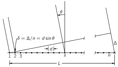
Some content on this page was disabled on June 17, 2020 as a result of a DMCA takedown notice from Michael A. Gottlieb, Rudolf Pfeiffer, and The California Institute of Technology. You can learn more about the DMCA here:

https://wordpress.com/support/copyright-and-the-dmca/
Some content on this page was disabled on June 17, 2020 as a result of a DMCA takedown notice from Michael A. Gottlieb, Rudolf Pfeiffer, and The California Institute of Technology. You can learn more about the DMCA here:
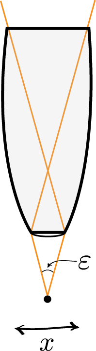
https://wordpress.com/support/copyright-and-the-dmca/