Playing with amplitudes

Pre-script (dated 26 June 2020): This post got mutilated by the removal of some material by the dark force. You should be able to follow the main story line, however. If anything, the lack of illustrations might actually help you to think things through for yourself. In any case, we now have different views on these concepts as part of our realist interpretation of quantum mechanics, so we recommend you read our recent papers instead of these old blog posts.

Original post:

Let’s play a bit with the stuff we found in our previous post. This is going to be unconventional, or experimental, if you want. The idea is to give you… Well… Some ideas. So you can play yourself. 🙂 Let’s go.

Let’s first look at Feynman’s (simplified) formula for the amplitude of a photon to go from point a to point b. If we identify point a by the position vector r₁ and point b by the position vector r₂, and using Dirac’s fancy bra-ket notation, then it’s written as:

So we have a vector dot product here: p∙r₁₂ = |p|∙|r₁₂|· cosθ = p∙r₁₂·cosα. The angle here (α) is the angle between the p and r₁₂ vector. All good. Well… No. We’ve got a problem. When it comes to calculating probabilities, the α angle doesn’t matter: |e^i·θ/r|² = 1/r². Hence, for the probability, we get: P = | 〈r₂|r₁〉 |² = 1/r₁₂². Always ! Now that’s strange. The θ = p∙r₁₂/ħ argument gives us a different phase depending on the angle (α) between p and r₁₂. But… Well… Think of it: cosα goes from 1 to 0 when α goes from 0 to ±90° and, of course, is negative when p and r₁₂ have opposite directions but… Well… According to this formula, the probabilities do not depend on the direction of the momentum. That’s just weird, I think. Did Feynman, in his iconic Lectures, give us a meaningless formula?

Maybe. We may also note this function looks like the elementary wavefunction for any particle, which we wrote as:

ψ(x, t) = a·e^−i∙θ = a·e^{−i∙(E∙t − p∙x)/ħ}= a·e^{−i∙(E∙t)/ħ}·e^{i∙(p∙x)/ħ}

The only difference is that the 〈r₂|r₁〉 sort of abstracts away from time, so… Well… Let’s get a feel for the quantities. Let’s think of a photon carrying some typical amount of energy. Hence, let’s talk visible light and, therefore, photons of a few eV only – say 5.625 eV = 5.625×1.6×10⁻¹⁹ J = 9×10⁻¹⁹ J. Hence, their momentum is equal to p = E/c = (9×10⁻¹⁹ N·m)/(3×10⁵ m/s) = 3×10⁻²⁴ N·s. That’s tiny but that’s only because newtons and seconds are enormous units at the (sub-)atomic scale. As for the distance, we may want to use the thickness of a playing card as a starter, as that’s what Young used when establishing the experimental fact of light interfering with itself. Now, playing cards in Young’s time were obviously rougher than those today, but let’s take the smaller distance: modern cards are as thin as 0.3 mm. Still, that distance is associated with a value of θ that is equal to 13.6 million. Hence, the density of our wavefunction is enormous at this scale, and it’s a bit of a miracle that Young could see any interference at all ! As shown in the table below, we only get meaningful values (remember: θ is a phase angle) when we go down to the nanometer scale (10⁻⁹ m) or, even better, the angstroms scale ((10⁻⁹ m). 

So… Well… Again: what can we do with Feynman’s formula? Perhaps he didn’t give us a propagator function but something that is more general (read: more meaningful) at our (limited) level of knowledge. As I’ve been reading Feynman for quite a while now – like three or four years 🙂 – I think… Well… Yes. That’s it. Feynman wants us to think about it. 🙂 Are you joking again, Mr. Feynman? 🙂 So let’s assume the reasonable thing: let’s assume it gives us the amplitude to go from point a to point b by the position vector along some path r. So, then, in line with what we wrote in our previous post, let’s say p·r (momentum over a distance) is the action (S) we’d associate with this particular path (r) and then see where we get. So let’s write the formula like this:

ψ = a·e^i·θ = (1/r)·e^i·S/ħ = e^i·p∙r/ħ/r

We’ll use an index to denote the various paths: r₀ is the straight-line path and r_i is any (other) path. Now, quantum mechanics tells us we should calculate this amplitude for every possible path. The illustration below shows the straight-line path and two nearby paths. So each of these paths is associated with some amount of action, which we measure in Planck units: θ = S/ħ. 

The time interval is given by t = t₀ = r₀/c, for all paths. Why is the time interval the same for all paths? Because we think of a photon going from some specific point in space and in time to some other specific point in space and in time. Indeed, when everything is said and done, we do think of light as traveling from point a to point b at the speed of light (c). In fact, all of the weird stuff here is all about trying to explain how it does that. 🙂

Now, if we would think of the photon actually traveling along this or that path, then this implies its velocity along any of the nonlinear paths will be larger than c, which is OK. That’s just the weirdness of quantum mechanics, and you should actually not think of the photon actually traveling along one of these paths anyway although we’ll often put it that way. Think of something fuzzier, whatever that may be. 🙂

So the action is energy times time, or momentum times distance. Hence, the difference in action between two paths i and j is given by:

δS = p·r_j − p·r_i = p·(r_j − r_i) = p·Δr

I’ll explain the δS < 2πħ/3 thing in a moment. Let’s first pause and think about the uncertainty and how we’re modeling it. We can effectively think of the variation in S as some uncertainty in the action: δS = ΔS = p·Δr. However, if S is also equal to energy times time (S = E·t), and we insist t is the same for all paths, then we must have some uncertainty in the energy, right? Hence, we can write δS as ΔS = ΔE·t. But, of course, E = E = m·c² = p·c, so we will have an uncertainty in the momentum as well. Hence, the variation in S should be written as:

δS = ΔS = Δp·Δr

That’s just logical thinking: if we, somehow, entertain the idea of a photon going from some specific point in spacetime to some other specific point in spacetime along various paths, then the variation, or uncertainty, in the action will effectively combine some uncertainty in the momentum and the distance. We can calculate Δp as ΔE/c, so we get the following:

δS = ΔS = Δp·Δr = ΔE·Δr/c = ΔE·Δt with Δt = Δr/c

So we have the two expressions for the Uncertainty Principle here: ΔS = Δp·Δr = ΔE·Δt. Just be careful with the interpretation of Δt: it’s just the equivalent of Δr. We just express the uncertainty in distance in seconds using the (absolute) speed of light. We are not changing our spacetime interval: we’re still looking at a photon going from a to b in t seconds, exactly. Let’s now look at the δS < 2πħ/3 thing. If we’re adding two amplitudes (two arrows or vectors, so to speak) and we want the magnitude of the result to be larger than the magnitude of the two contributions, then the angle between them should be smaller than 120 degrees, so that’s 2π/3 rad. The illustration below shows how you can figure that out geometrically.Hence, if S₀ is the action for r₀, then S₁ = S₀ + ħ and S₂ = S₀ + 2·ħ are still good, but S₃ = S₀ + 3·ħ is not good. Why? Because the difference in the phase angles is Δθ = S₁/ħ − S₀/ħ = (S₀ + ħ)/ħ − S₀/ħ = 1 and Δθ = S₂/ħ − S₀/ħ = (S₀ + 2·ħ)/ħ − S₀/ħ = 2 respectively, so that’s 57.3° and 114.6° respectively and that’s, effectively, less than 120°. In contrast, for the next path, we find that Δθ = S₃/ħ − S₀/ħ = (S₀ + 3·ħ)/ħ − S₀/ħ = 3, so that’s 171.9°. So that amplitude gives us a negative contribution.

Let’s do some calculations using a spreadsheet. To simplify things, we will assume we measure everything (time, distance, force, mass, energy, action,…) in Planck units. Hence, we can simply write: S_n = S₀ + n. Of course, n = 1, 2,… etcetera, right? Well… Maybe not. We are measuring action in units of ħ, but do we actually think action comes in units of ħ? I am not sure. It would make sense, intuitively, but… Well… There’s uncertainty on the energy (E) and the momentum (p) of our photon, right? And how accurately can we measure the distance? So there’s some randomness everywhere. 😦 So let’s leave that question open as for now.

We will also assume that the phase angle for S₀ is equal to 0 (or some multiple of 2π, if you want). That’s just a matter of choosing the origin of time. This makes it really easy: ΔS_n = S_n − S₀ = n, and the associated phase angle θ_n = Δθ_n is the same. In short, the amplitude for each path reduces to ψ_n = e^i·n/r₀. So we need to add these first and then calculate the magnitude, which we can then square to get a probability. Of course, there is also the issue of normalization (probabilities have to add up to one) but let’s tackle that later. For the calculations, we use Euler’s r·e^i·θ = r·(cosθ + i·sinθ) = r·cosθ + i·r·sinθ formula. Needless to say, |r·e^i·θ|² = |r|²·|e^i·θ|² = |r|²·(cos²θ + sin²θ) = r. Finally, when adding complex numbers, we add the real and imaginary parts respectively, and we’ll denote the ψ₀ + ψ₁ +ψ₂ + … sum as Ψ.

Now, we also need to see how our ΔS = Δp·Δr works out. We may want to assume that the uncertainty in p and in r will both be proportional to the overall uncertainty in the action. For example, we could try writing the following: ΔS_n = Δp_n·Δr_n = n·Δp₁·Δr₁. It also makes sense that you may want Δp_n and Δr_n to be proportional to Δp₁ and Δr₁ respectively. Combining both, the assumption would be this:

Δp_n = √n·Δp₁ and Δr_n = √n·Δr₁

So now we just need to decide how we will distribute ΔS₁ = ħ = 1 over Δp₁ and Δr₁ respectively. For example, if we’d assume Δp₁ = 1, then Δr₁ = ħ/Δp₁ = 1/1 = 1. These are the calculations. I will let you analyze them. 🙂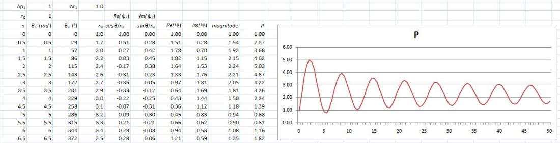Well… We get a weird result. It reminds me of Feynman’s explanation of the partial reflection of light, shown below, but… Well… That doesn’t make much sense, does it?

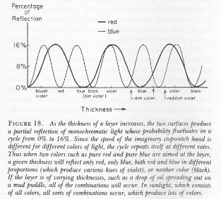
Hmm… Maybe it does. 🙂 Look at the graph more carefully. The peaks sort of oscillate out so… Well… That might make sense… 🙂

Does it? Are we doing something wrong here? These amplitudes should reflect the ones that are reflected in those nice animations (like this one, for example, which is part of that’s part of the Wikipedia article on Feynman’s path integral formulation of quantum mechanics). So what’s wrong, if anything? Well… Our paths differ by some fixed amount of action, which doesn’t quite reflect the geometric approach that’s used in those animations. The graph below shows how the distance r varies as a function of n. 

If we’d use a model in which the distance would increase linearly or, preferably, exponentially, then we’d get the result we want to get, right?

Well… Maybe. Let’s try it. Hmm… We need to think about the geometry here. Look at the triangle below. 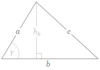If b is the straight-line path (r₀), then ac could be one of the crooked paths (r_n). To simplify, we’ll assume isosceles triangles, so a equals c and, hence, r_n = 2·a = 2·c. We will also assume the successive paths are separated by the same vertical distance (h = h₁) right in the middle, so h_b = h_n = n·h₁. It is then easy to show the following:This gives the following graph for r_n = 10 and h₁ = 0.01.

Is this the right step increase? Not sure. We can vary the values in our spreadsheet. Let’s first build it. The photon will have to travel faster in order to cover the extra distance in the same time, so its momentum will be higher. Let’s think about the velocity. Let’s start with the first path (n = 1). In order to cover the extra distance Δr₁, the velocity c₁ must be equal to (r₀ + Δr₁)/t = r₀/t + Δr₁/t = c + Δr₁/t = c₀ + Δr₁/t. We can write c₁ as c₁ = c₀ + Δc₁, so Δc₁ = Δr₁/t. Now, the ratio of p₁  and p₀ will be equal to the ratio of c₁ and c₀ because p₁/p₀ = (mc₁)/mc₀) = c₁/c₀. Hence, we have the following formula for p₁:

p₁ = p₀·c₁/c₀ = p₀·(c₀ + Δc₁)/c₀ = p₀·[1 + Δr₁/(c₀·t) = p₀·(1 + Δr₁/r₀)

For p_n, the logic is the same, so we write:

p_n = p₀·c_n/c₀ = p₀·(c₀ + Δc_n)/c₀ = p₀·[1 + Δr_n/(c₀·t) = p₀·(1 + Δr_n/r₀)

Let’s do the calculations, and let’s use meaningful values, so the nanometer scale and actual values for Planck’s constant and the photon momentum. The results are shown below.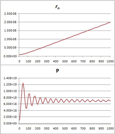 

Pretty interesting. In fact, this looks really good. The probability first swings around wildly, because of these zones of constructive and destructive interference, but then stabilizes. [Of course, I would need to normalize the probabilities, but you get the idea, right?] So… Well… I think we get a very meaningful result with this model. Sweet ! 🙂 I’m lovin’ it ! 🙂 And, here you go, this is (part of) the calculation table, so you can see what I am doing. 🙂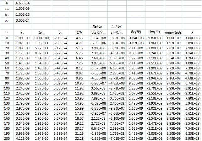

The graphs below look even better: I just changed the h₁/r₀ ratio from 1/100 to 1/10. The probability stabilizes almost immediately. 🙂 So… Well… It’s not as fancy as the referenced animation, but I think the educational value of this thing here is at least as good ! 🙂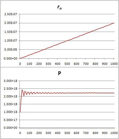

🙂 This is good stuff… 🙂

Post scriptum (19 September 2017): There is an obvious inconsistency in the model above, and in the calculations. We assume there is a path r₁ = , r₂, r₂,etcetera, and then we calculate the action for it, and the amplitude, and then we add the amplitude to the sum. But, surely, we should count these paths twice, in two-dimensional space, that is. Think of the graph: we have positive and negative interference zones that are sort of layered around the straight-line path, as shown below.

In three-dimensional space, these lines become surfaces. Hence, rather than adding one arrow for every δ  having one contribution only, we may want to add… Well… In three-dimensional space, the formula for the surface around the straight-line path would probably look like π·h_n·r₁, right? Hmm… Interesting idea. I changed my spreadsheet to incorporate that idea, and I got the graph below. It’s a nonsensical result, because the probability does swing around, but it gradually spins out of control: it never stabilizes.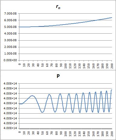That’s because we increase the weight of the paths that are further removed from the center. So… Well… We shouldn’t be doing that, I guess. 🙂 I’ll you look for the right formula, OK? Let me know when you found it. 🙂

Some content on this page was disabled on June 16, 2020 as a result of a DMCA takedown notice from The California Institute of Technology. You can learn more about the DMCA here:

https://en.support.wordpress.com/copyright-and-the-dmca/