Post scriptum note added on 11 July 2016: This is one of the more speculative posts which led to my e-publication analyzing the wavefunction as an energy propagation. With the benefit of hindsight, I would recommend you to immediately read the more recent exposé on the matter that is being presented here, which you can find by clicking on the provided link.
Original post:
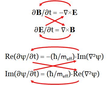
This post is, essentially, a continuation of my previous post, in which I juxtaposed the following images:


Both are the same, and then they’re not. The illustration on the right-hand side is a regular quantum-mechanical wavefunction, i.e. an amplitude wavefunction. You’ve seen that one before. In this case, the x-axis represents time, so we’re looking at the wavefunction at some particular point in space. ]You know we can just switch the dimensions and it would all look the same.] The illustration on the left-hand side looks similar, but it’s not an amplitude wavefunction. The animation shows how the electric field vector (E) of an electromagnetic wave travels through space. Its shape is the same. So it’s the same function. Is it also the same reality?
Yes and no. And I would say: more no than yes—in this case, at least. Note that the animation does not show the accompanying magnetic field vector (B). That vector is equally essential in the electromagnetic propagation mechanism according to Maxwell’s equations, which—let me remind you—are equal to:
- ∂B/∂t = –∇×E
- ∂E/∂t = ∇×B
In fact, I should write the second equation as ∂E/∂t = c2∇×B, but then I assume we measure time and distance in equivalent units, so c = 1.
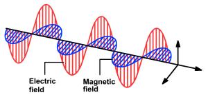
You know that E and B are two aspects of one and the same thing: if we have one, then we have the other. To be precise, B is always orthogonal to E in the direction that’s given by the right-hand rule for the following vector cross-product: B = ex×E, with ex the unit vector pointing in the x-direction (i.e. the direction of propagation). The reality behind is illustrated below for a linearly polarized electromagnetic wave.

The B = ex×E equation is equivalent to writing B= i·E, which is equivalent to:
B = i·E = ei(π/2)·ei(kx − ωt) = cos(kx − ωt + π/2) + i·sin(kx − ωt + π/2)
= −sin((kx − ωt) + i·cos(kx − ωt)
Now, E and B have only two components: Ey and Ez, and By and Bz. That’s only because we’re looking at some ideal or elementary electromagnetic wave here but… Well… Let’s just go along with it. 🙂 It is then easy to prove that the equation above amounts to writing:
- By = cos(kx − ωt + π/2) = −sin(kx − ωt) = −Ez
- Bz = sin(kx − ωt + π/2) = cos(kx − ωt) = Ey
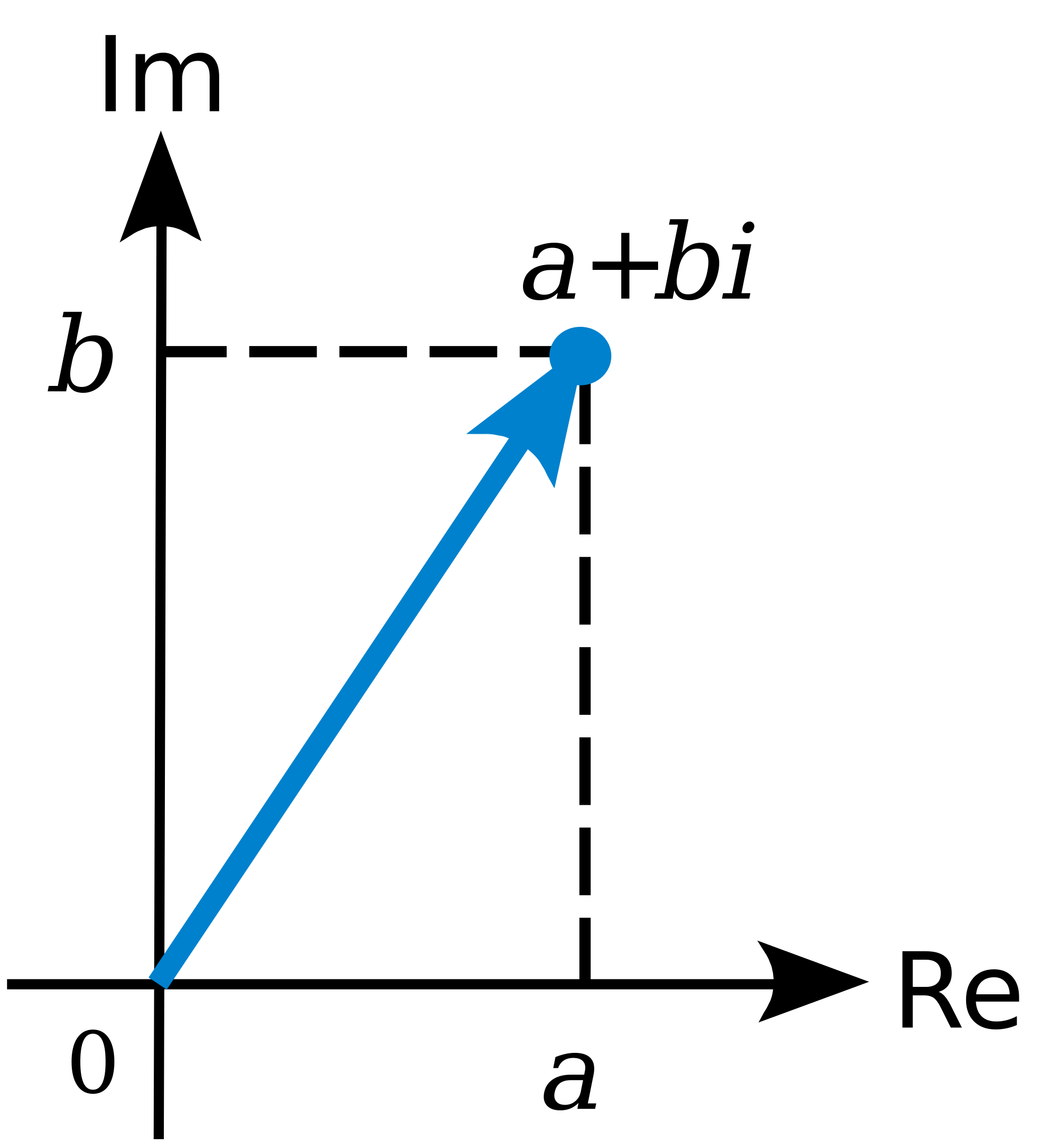
We should now think of Ey and Ez as the real and imaginary part of some wavefunction, which we’ll denote as ψE = ei(kx − ωt). So we write:
E = (Ey, Ez) = Ey + i·Ez = cos(kx − ωt) + i∙sin(kx − ωt) = Re(ψE) + i·Im(ψE) = ψE = ei(kx − ωt)
What about B? We just do the same, so we write:
B = (By, Bz) = By + i·Bz = ψB = i·E = i·ψE = −sin(kx − ωt) + i∙sin(kx − ωt) = − Im(ψE) + i·Re(ψE)
Now we need to prove that ψE and ψB are regular wavefunctions, which amounts to proving Schrödinger’s equation, i.e. ∂ψ/∂t = i·(ħ/m)·∇2ψ, for both ψE and ψB. [Note I use the Schrödinger’s equation for a zero-mass spin-zero particle here, which uses the ħ/m factor rather than the ħ/(2m) factor.] To prove that ψE and ψB are regular wavefunctions, we should prove that:
- Re(∂ψE/∂t) = −(ħ/m)·Im(∇2ψE) and Im(∂ψE/∂t) = (ħ/m)·Re(∇2ψE), and
- Re(∂ψB/∂t) = −(ħ/m)·Im(∇2ψB) and Im(∂ψB/∂t) = (ħ/m)·Re(∇2ψB).
Let’s do the calculations for the second pair of equations. The time derivative on the left-hand side is equal to:
∂ψB/∂t = −iω·iei(kx − ωt) = ω·[cos(kx − ωt) + i·sin(kx − ωt)] = ω·cos(kx − ωt) + iω·sin(kx − ωt)
The second-order derivative on the right-hand side is equal to:
∇2ψB = ∂2ψB/∂x2 = i·k2·ei(kx − ωt) = k2·cos(kx − ωt) + i·k2·sin(kx − ωt)
So the two equations for ψB are equivalent to writing:
- Re(∂ψB/∂t) = −(ħ/m)·Im(∇2ψB) ⇔ ω·cos(kx − ωt) = k2·(ħ/m)·cos(kx − ωt)
- Im(∂ψB/∂t) = (ħ/m)·Re(∇2ψB) ⇔ ω·sin(kx − ωt) = k2·(ħ/m)·sin(kx − ωt)
So we see that both conditions are fulfilled if, and only if, ω = k2·(ħ/m).
Now, we also demonstrated in that post of mine that Maxwell’s equations imply the following:
- ∂By/∂t = –(∇×E)y = ∂Ez/∂x = ∂[sin(kx − ωt)]/∂x = k·cos(kx − ωt) = k·Ey
- ∂Bz/∂t = –(∇×E)z = – ∂Ey/∂x = – ∂[cos(kx − ωt)]/∂x = k·sin(kx − ωt) = k·Ez
Hence, using those By = −Ez and Bz = Ey equations above, we can also calculate these derivatives as:
- ∂By/∂t = −∂Ez/∂t = −∂sin(kx − ωt)/∂t = ω·cos(kx − ωt) = ω·Ey
- ∂Bz/∂t = ∂Ey/∂t = ∂cos(kx − ωt)/∂t = −ω·[−sin(kx − ωt)] = ω·Ez
In other words, Maxwell’s equations imply that ω = k, which is consistent with us measuring time and distance in equivalent units, so the phase velocity is c = 1 = ω/k.
So far, so good. We basically established that the propagation mechanism for an electromagnetic wave, as described by Maxwell’s equations, is fully coherent with the propagation mechanism—if we can call it like that—as described by Schrödinger’s equation. We also established the following equalities:
- ω = k
- ω = k2·(ħ/m)
The second of the two de Broglie equations tells us that k = p/ħ, so we can combine these two equations and re-write these two conditions as:
ω/k = 1 = k·(ħ/m) = (p/ħ)·(ħ/m) = p/m ⇔ p = m
What does this imply? The p here is the momentum: p = m·v, so this condition implies v must be equal to 1 too, so the wave velocity is equal to the speed of light. Makes sense, because we actually are talking light here. 🙂 In addition, because it’s light, we also know E/p = c = 1, so we have – once again – the general E = p = m equation, which we’ll need!
OK. Next. Let’s write the Schrödinger wave equation for both wavefunctions:
- ∂ψE/∂t = i·(ħ/mE)·∇2ψE, and
- ∂ψB/∂t = i·(ħ/mB)·∇2ψB.
Huh? What’s mE and mE? We should only associate one mass concept with our electromagnetic wave, shouldn’t we? Perhaps. I just want to be on the safe side now. Of course, if we distinguish mE and mB, we should probably also distinguish pE and pB, and EE and EB as well, right? Well… Yes. If we accept this line of reasoning, then the mass factor in Schrödinger’s equations is pretty much like the 1/c2 = μ0ε0 factor in Maxwell’s (1/c2)·∂E/∂t = ∇×B equation: the mass factor appears as a property of the medium, i.e. the vacuum here! [Just check my post on physical constants in case you wonder what I am trying to say here, in which I explain why and how c defines the (properties of the) vacuum.]
To be consistent, we should also distinguish pE and pB, and EE and EB, and so we should write ψE and ψB as:
- ψE = ei(kEx − ωEt), and
- ψB = ei(kBx − ωBt).
Huh? Yes. I know what you think: we’re talking one photon—or one electromagnetic wave—so there can be only one energy, one momentum and, hence, only one k, and one ω. Well… Yes and no. Of course, the following identities should hold: kE = kB and, likewise, ωE = ωB. So… Yes. They’re the same: one k and one ω. But then… Well… Conceptually, the two k’s and ω’s are different. So we write:
- pE = EE = mE, and
- pB = EB = mB.
The obvious question is: can we just add them up to find the total energy and momentum of our photon? The answer is obviously positive: E = EE + EB, p = pE + pB and m = mE + mB.
Let’s check a few things now. How does it work for the phase and group velocity of ψE and ψB? Simple:
- vg = ∂ωE/∂kE = ∂[EE/ħ]/∂[pE/ħ] = ∂EE/∂pE = ∂pE/∂pE = 1
- vp = ωE/kE = (EE/ħ)/(pE/ħ) = EE/pE = pE/pE = 1
So we’re fine, and you can check the result for ψB by substituting the subscript E for B. To sum it all up, what we’ve got here is the following:
- We can think of a photon having some energy that’s equal to E = p = m (assuming c = 1), but that energy would be split up in an electric and a magnetic wavefunction respectively: ψE and ψB.
- Schrödinger’s equation applies to both wavefunctions, but the E, p and m in those two wavefunctions are the same and not the same: their numerical value is the same (pE =EE = mE = pB =EB = mB), but they’re conceptually different. They must be: if not, we’d get a phase and group velocity for the wave that doesn’t make sense.
Of course, the phase and group velocity for the sum of the ψE and ψB waves must also be equal to c. This is obviously the case, because we’re adding waves with the same phase and group velocity c, so there’s no issue with the dispersion relation.
So let’s insert those pE =EE = mE = pB =EB = mB values in the two wavefunctions. For ψE, we get:
ψE = ei[kEx − ωEt) = ei[(pE/ħ)·x − (EE/ħ)·t]
You can do the calculation for ψB yourself. Let’s simplify our life a little bit and assume we’re using Planck units, so ħ = 1, and so the wavefunction simplifies to ψE = ei·(pE·x − EE·t). We can now add the components of E and B using the summation formulas for sines and cosines:
1. By + Ey = cos(pB·x − EB·t + π/2) + cos(pE·x − EE·t) = 2·cos[(p·x − E·t + π/2)/2]·cos(π/4) = √2·cos(p·x/2 − E·t/2 + π/4)
2. Bz + Ez = sin(pB·x − EB·t+π/2) + sin(pE·x − EE·t) = 2·sin[(p·x − E·t + π/2)/2]·cos(π/4) = √2·sin(p·x/2 − E·t/2 + π/4)
Interesting! We find a composite wavefunction for our photon which we can write as:
E + B = ψE + ψB = E + i·E = √2·ei(p·x/2 − E·t/2 + π/4) = √2·ei(π/4)·ei(p·x/2 − E·t/2) = √2·ei(π/4)·E
What a great result! It’s easy to double-check, because we can see the E + i·E = √2·ei(π/4)·E formula implies that 1 + i should equal √2·ei(π/4). Now that’s easy to prove, both geometrically (just do a drawing) or formally: √2·ei(π/4) = √2·cos(π/4) + i·sin(π/4ei(π/4) = (√2/√2) + i·(√2/√2) = 1 + i. We’re bang on! 🙂
We can double-check once more, because we should get the same from adding E and B = i·E, right? Let’s try:
E + B = E + i·E = cos(pE·x − EE·t) + i·sin(pE·x − EE·t) + i·cos(pE·x − EE·t) − sin(pE·x − EE·t)
= [cos(pE·x − EE·t) – sin(pE·x − EE·t)] + i·[sin(pE·x − EE·t) – cos(pE·x − EE·t)]
Indeed, we can see we’re going to obtain the same result, because the −sinθ in the real part of our composite wavefunction is equal to cos(θ+π/2), and the −cosθ in its imaginary part is equal to sin(θ+π/2). So the sum above is the same sum of cosines and sines that we did already.
So our electromagnetic wavefunction, i.e. the wavefunction for the photon, is equal to:
ψ = ψE + ψB = √2·ei(p·x/2 − E·t/2 + π/4) = √2·ei(π/4)·ei(p·x/2 − E·t/2)
What about the √2 factor in front, and the π/4 term in the argument itself? No sure. It must have something to do with the way the magnetic force works, which is not like the electric force. Indeed, remember the Lorentz formula: the force on some unit charge (q = 1) will be equal to F = E + v×B. So… Well… We’ve got another cross-product here and so the geometry of the situation is quite complicated: it’s not like adding two forces F1 and F2 to get some combined force F = F1 and F2.
In any case, we need the energy, and we know that its proportional to the square of the amplitude, so… Well… We’re spot on: the square of the √2 factor in the √2·cos product and √2·sin product is 2, so that’s twice… Well… What? Hold on a minute! We’re actually taking the absolute square of the E + B = ψE + ψB = E + i·E = √2·ei(p·x/2 − E·t/2 + π/4) wavefunction here. Is that legal? I must assume it is—although… Well… Yes. You’re right. We should do some more explaining here.
We know that we usually measure the energy as some definite integral, from t = 0 to some other point in time, or over the cycle of the oscillation. So what’s the cycle here? Our combined wavefunction can be written as √2·ei(p·x/2 − E·t/2 + π/4) = √2·ei(θ/2 + π/4), so a full cycle would correspond to θ going from 0 to 4π here, rather than from 0 to 2π. So that explains the √2 factor in front of our wave equation.
Bingo! If you were looking for an interpretation of the Planck energy and momentum, here it is. And, while everything that’s written above is not easy to understand, it’s close to the ‘intuitive’ understanding to quantum mechanics that we were looking for, isn’t it? The quantum-mechanical propagation model explains everything now. 🙂 I only need to show one more thing, and that’s the different behavior of bosons and fermions:
- The amplitudes of identitical bosonic particles interfere with a positive sign, so we have Bose-Einstein statistics here. As Feynman writes it: (amplitude direct) + (amplitude exchanged).
- The amplitudes of identical fermionic particles interfere with a negative sign, so we have Fermi-Dirac statistics here: (amplitude direct) − (amplitude exchanged).
I’ll think about it. I am sure it’s got something to do with that B= i·E formula or, to put it simply, with the fact that, when bosons are involved, we get two wavefunctions (ψE and ψB) for the price of one. The reasoning should be something like this:
I. For a massless particle (i.e. a zero-mass fermion), our wavefunction is just ψ = ei(p·x − E·t). So we have no √2 or √2·ei(π/4) factor in front here. So we can just add any number of them – ψ1 + ψ2 + ψ3 + … – and then take the absolute square of the amplitude to find a probability density, and we’re done.
II. For a photon (i.e. a zero-mass boson), our wavefunction is √2·ei(π/4)·ei(p·x − E·t)/2, which – let’s introduce a new symbol – we’ll denote by φ, so φ = √2·ei(π/4)·ei(p·x − E·t)/2. Now, if we add any number of these, we get a similar sum but with that √2·ei(π/4) factor in front, so we write: φ1 + φ2 + φ3 + … = √2·ei(π/4)·(ψ1 + ψ2 + ψ3 + …). If we take the absolute square now, we’ll see the probability density will be equal to twice the density for the ψ1 + ψ2 + ψ3 + … sum, because
|√2·ei(π/4)·(ψ1 + ψ2 + ψ3 + …)|2 = |√2·ei(π/4)|2·|ψ1 + ψ2 + ψ3 + …)|2 = 2·|ψ1 + ψ2 + ψ3 + …)|2
So… Well… I still need to connect this to Feynman’s (amplitude direct) ± (amplitude exchanged) formula, but I am sure it can be done.
Now, we haven’t tested the complete √2·ei(π/4)·ei(p·x − E·t)/2 wavefunction. Does it respect Schrödinger’s ∂ψ/∂t = i·(1/m)·∇2ψ or, including the 1/2 factor, the ∂ψ/∂t = i·[1/2m)]·∇2ψ equation? [Note we assume, once again, that ħ = 1, so we use Planck units once more.] Let’s see. We can calculate the derivatives as:
- ∂ψ/∂t = −√2·ei(π/4)·e−i∙[p·x − E·t]/2·(i·E/2)
- ∇2ψ = ∂2[√2·ei(π/4)·e−i∙[p·x − E·t]/2]/∂x2 = √2·ei(π/4)·∂[√2·ei(π/4)·e−i∙[p·x − E·t]/2·(i·p/2)]/∂x = −√2·ei(π/4)·e−i∙[p·x − E·t]/2·(p2/4)
So Schrödinger’s equation becomes:
−i·√2·ei(π/4)·e−i∙[p·x − E·t]/2·(i·E/2) = −i·(1/m)·√2·ei(π/4)·e−i∙[p·x − E·t]/2·(p2/4) ⇔ 1/2 = 1/4!?
That’s funny ! It doesn’t work ! The E and m and p2 are OK because we’ve got that E = m = p equation, but we’ve got problems with yet another factor 2. It only works when we use the 2/m coefficient in Schrödinger’s equation.
So… Well… There’s no choice. That’s what we’re going to do. The Schrödinger equation for the photon is ∂ψ/∂t = i·(2/m)·∇2ψ !
It’s a very subtle point. This is all great, and very fundamental stuff! Let’s now move on to Schrödinger’s actual equation, i.e. the ∂ψ/∂t = i·(ħ/2m)·∇2ψ equation.
Post scriptum on the Planck units:
If we measure time and distance in equivalent units, say seconds, we can re-write the quantum of action as:
1.0545718×10⁻³⁴ N·m·s = (1.21×1044 N)·(1.6162×10⁻³⁵ m)·(5.391×10−44 s)
⇔ (1.0545718×10⁻³⁴/2.998×108) N·s2 = (1.21×1044 N)·(1.6162×10⁻³⁵/2.998×108 s)(5.391×10−44 s)
⇔ (1.21×1044 N) = [(1.0545718×10⁻³⁴/2.998×108)]/[(1.6162×10−35/2.998×108 s)(5.391×10−44 s)] N·s2/s2
You’ll say: what’s this? Well… Look at it. We’ve got a much easier formula for the Planck force—much easier than the standard formulas you’ll find on Wikipedia, for example. If we re-interpret the symbols ħ and c so they denote the numerical value of the quantum of action and the speed of light in standard SI units (i.e. newton, meter and second)—so ħ and c become dimensionless, or mathematical constants only, rather than physical constants—then the formula above can be written as:
FP newton = (ħ/c)/[(lP/c)·tP] newton ⇔ FP = ħ/(lP·tP)
Just double-check it: 1.0545718×10⁻³⁴/(1.6162×10−35·5.391×10−44) = 1.21×1044. Bingo!
You’ll say: what’s the point? The point is: our model is complete. We don’t need the other physical constants – i.e. the Coulomb, Boltzmann and gravitational constant – to calculate the Planck units we need, i.e. the Planck force, distance and time units. It all comes out of our elementary wavefunction! All we need to explain the Universe – or, let’s be more modest, quantum mechanics – is two numerical constants (c and ħ) and Euler’s formula (which uses π and e, of course). That’s it.
If you don’t think that’s a great result, then… Well… Then you’re not reading this. 🙂


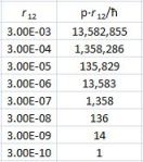
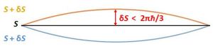
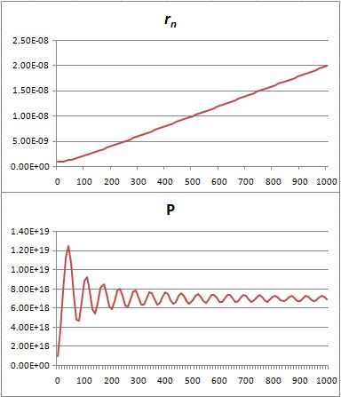
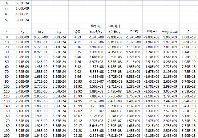
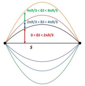
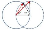 Hence, if S0 is the action for r0, then S1 = S0 + ħ and S2 = S0 + 2·ħ are still good, but S3 = S0 + 3·ħ is not good. Why? Because the difference in the phase angles is Δθ = S1/ħ − S0/ħ = (S0 + ħ)/ħ − S0/ħ = 1 and Δθ = S2/ħ − S0/ħ = (S0 + 2·ħ)/ħ − S0/ħ = 2 respectively, so that’s 57.3° and 114.6° respectively and that’s, effectively, less than 120°. In contrast, for the next path, we find that Δθ = S3/ħ − S0/ħ = (S0 + 3·ħ)/ħ − S0/ħ = 3, so that’s 171.9°. So that amplitude gives us a negative contribution.
 Well… We get a weird result. It reminds me of
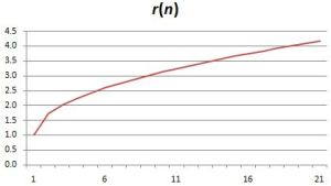
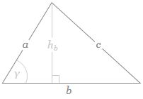 If b is the straight-line path (r0), then ac could be one of the crooked paths (rn). To simplify, we’ll assume isosceles triangles, so a equals c and, hence, rn = 2·a = 2·c. We will also assume the successive paths are separated by the same vertical distance (h = h1) right in the middle, so hb = hn = n·h1. It is then easy to show the following:
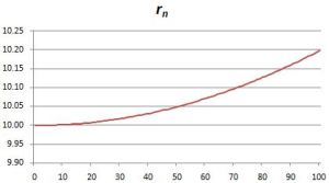

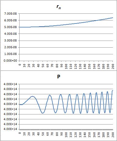 That’s because we increase the weight of the paths that are further removed from the center. So… Well… We shouldn’t be doing that, I guess. 🙂 I’ll you look for the right formula, OK? Let me know when you found it. 🙂