The Complementarity Principle

Pre-script (dated 26 June 2020): This post has become less relevant because my views on all things quantum-mechanical have evolved significantly as a result of my progression towards a more complete realist (classical) interpretation of quantum physics. Hence, we recommend you read our recent papers. I keep blog posts like these mainly because I want to keep track of where I came from. I might review them one day, but I currently don’t have the time or energy for it. 🙂

Original post:

Unlike what you might think when seeing the title of this post, it is not my intention to enter into philosophical discussions here: many authors have been writing about this ‘principle’, most of which–according to eminent physicists–don’t know what they are talking about. So I have no intention to make a fool of myself here too. However, what I do want to do here is explore, in an intuitive way, how the classical and quantum-mechanical explanations of the phenomenon of the diffraction of light are different from each other–and fundamentally so–while, necessarily, having to yield the same predictions. It is in that sense that the two explanations should be ‘complementary’.

The classical explanation

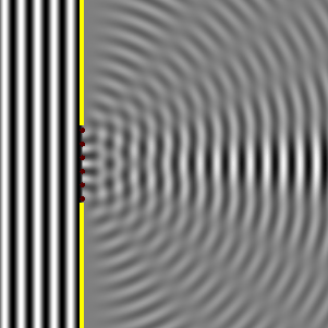
I’ve done a fairly complete analysis of the classical explanation in my posts on Diffraction and the Uncertainty Principle (20 and 21 September), so I won’t dwell on that here. Let me just repeat the basics. The model is based on the so-called Huygens-Fresnel Principle, according to which each point in the slit becomes a source of a secondary spherical wave. These waves then interfere, constructively or destructively, and, hence, by adding them, we get the form of the wave at each point of time and at each point in space behind the slit. The animation below illustrates the idea. However, note that the mathematical analysis does not assume that the point sources are neatly separated from each other: instead of only six point sources, we have an infinite number of them and, hence, adding up the waves amounts to solving some integral (which, as you know, is an infinite sum).

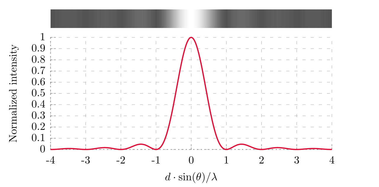
We know what we are supposed to get: a diffraction pattern. The intensity of the light on the screen at the other side depends on (1) the slit width (d), (2) the frequency of the light (λ), and (3) the angle of incidence (θ), as shown below.

One point to note is that we have smaller bumps left and right. We don’t get that if we’d treat the slit as a single point source only, like Feynman does when he discusses the double-slit experiment for (physical) waves. Indeed, look at the image below: each of the slits acts as one point source only and, hence, the intensity curves I₁ and I₂ do not show a diffraction pattern. They are just nice Gaussian “bell” curves, albeit somewhat adjusted because of the angle of incidence (we have two slits above and below the center, instead of just one on the normal itself). So we have an interference pattern on the screen and, now that we’re here, let me be clear on terminology: I am going along with the widespread definition of diffraction being a pattern created by one slit, and the definition of interference as a pattern created by two or more slits. I am noting this just to make sure there’s no confusion.

That should be clear enough. Let’s move on the quantum-mechanical explanation.

The quantum-mechanical explanation

There are several formulations of quantum mechanics: you’ve heard about matrix mechanics and wave mechanics. Roughly speaking, in matrix mechanics “we interpret the physical properties of particles as matrices that evolve in time”, while the wave mechanics approach is primarily based on these complex-valued wave functions–one for each physical property (e.g. position, momentum, energy). Both approaches are mathematically equivalent.

There is also a third approach, which is referred to as the path integral formulation, which  “replaces the classical notion of a single, unique trajectory for a system with a sum, or functional integral, over an infinity of possible trajectories to compute an amplitude” (all definitions here were taken from Wikipedia). This approach is associated with Richard Feynman but can also be traced back to Paul Dirac, like most of the math involved in quantum mechanics, it seems. It’s this approach which I’ll try to explain–again, in an intuitive way only–in order to show the two explanations should effectively lead to the same predictions.

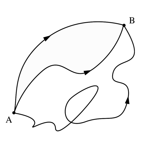
The key to understanding the path integral formulation is the assumption that a particle–and a ‘particle’ may refer to both bosons (e.g. photons) or fermions (e.g. electrons)–can follow any path from point A to B, as illustrated below. Each of these paths is associated with a (complex-valued) probability amplitude, and we have to add all these probability amplitudes to arrive at the probability amplitude for the particle to move from A to B.

You can find great animations illustrating what it’s all about in the relevant Wikipedia article but, because I can’t upload video here, I’ll just insert two illustrations from Feynman’s 1985 QED, in which he does what I try to do, and that is to approach the topic intuitively, i.e. without too much mathematical formalism. So probability amplitudes are just ‘arrows’ (with a length and a direction, just like a complex number or a vector), and finding the resultant or final arrow is a matter of just adding all the little arrows to arrive at one big arrow, which is the probability amplitude, which he denotes as P(A, B), as shown below.

This intuitive approach is great and actually goes a very long way in explaining complicated phenomena, such as iridescence for example (the wonderful patterns of color on an oil film!), or the partial reflection of light by glass (anything between 0 and 16%!). All his tricks make sense. For example, different frequencies are interpreted as slower or faster ‘stopwatches’ and, as such, they determine the final direction of the arrows which, in turn, explains why blue and red light are reflected differently. And so on and son. It all works. […] Up to a point.

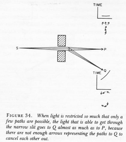
Indeed, Feynman does get in trouble when trying to explain diffraction. I’ve reproduced his explanation below. The key to the argument is the following:

1. If we have a slit that’s very wide, there are a lot of possible paths for the photon to take. However, most of these paths cancel each other out, and so that’s why the photon is likely to travel in a straight line. Let me quote Feynman: “When the gap between the blocks is wide enough to allow many neighboring paths to P and Q, the arrows for the paths to P add up (because all the paths to P take nearly the same time), while the paths to Q cancel out (because those paths have a sizable difference in time). So the photomultiplier at Q doesn’t click.” (QED, p.54)
2. However, “when the gap is nearly closed and there are only a few neighboring paths, the arrows to Q also add up, because there is hardly any difference in time between them, either (see Fig. 34). Of course, both final arrows are small, so there’s not much light either way through such a small hole, but the detector at Q clicks almost as much as the one at P! So when you try to squeeze light too much to make sure it’s going only in a straight line, it refuses to cooperate and begins to spread out.” (QED, p. 55)

This explanation is as simple and intuitive as Feynman’s ‘explanation’ of diffraction using the Uncertainty Principle in his introductory chapter on quantum mechanics (Lectures, I-38-2), which is illustrated below. I won’t go into the detail (I’ve done that before) but you should note that, just like the explanation above, such explanations do not explain the secondary, tertiary etc bumps in the diffraction pattern.

So what’s wrong with these explanations? Nothing much. They’re simple and intuitive, but essentially incomplete, because they do not incorporate all of the math involved in interference. Incorporating the math means doing these integrals for

1. Electromagnetic waves in classical mechanics: here we are talking ‘wave functions’ with some real-valued amplitude representing the strength of the electric and magnetic field; and
2. Probability waves: these are complex-valued functions, with the complex-valued amplitude representing probability amplitudes.

The two should, obviously, yield the same result, but a detailed comparison between the approaches is quite complicated, it seems. Now, I’ve googled a lot of stuff, and I duly note that diffraction of electromagnetic waves (i.e. light) is conveniently analyzed by summing up complex-valued waves too, and, moreover, they’re of the same familiar type: ψ = Ae^i(kx–ωt). However, these analyses also duly note that it’s only the real part of the wave that has an actual physical interpretation, and that it’s only because working with natural exponentials (addition, multiplication, integration, derivation, etc) is much easier than working with sine and cosine waves that such complex-valued wave functions are used (also) in classical mechanics. In fact, note the fine print in Feynman’s illustration of interference of physical waves (Fig. 37-2): he calculates the intensities I₁ and I₂ by taking the square of the absolute amplitudes ĥ₁ and ĥ₂, and the hat indicates that we’re also talking some complex-valued wave function here.

Hence, we must be talking the same mathematical waves in both explanations, aren’t we? In other words, we should get the same psi functions ψ = Ae^i(kx–ωt) in both explanations, don’t we? Well… Maybe. But… Probably not. As far as I know–but I must be wrong–we cannot just re-normalize the E and B vectors in these electromagnetic waves in order to establish an equivalence with probability waves. I haven’t seen that being done (but I readily admit I still have a lot of reading to do) and so I must assume it’s not very clear-cut at all.

So what? Well… I don’t know. So far, I did not find a ‘nice’ or ‘intuitive’ explanation of a quantum-mechanical approach to the phenomenon of diffraction yielding the same grand diffraction equation, referred to as the Fresnel-Kirchoff diffraction formula (see below), or one of its more comprehensible (because simplified) representations, such as the Fraunhofer diffraction formula, or the even easier formula which I used in my own post (you can google them: they’re somewhat less monstrous and–importantly–they work with real numbers only, which makes them easier to understand).

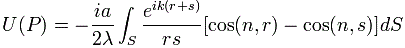[…] That looks pretty daunting, isn’t it? You may start to understand it a bit better by noting that (n, r) and (n, s) are angles, so that’s OK in a cosine function. The other variables also have fairly standard interpretations, as shown below, but… Admit it: ‘easy’ is something else, isn’t it?

So… Where are we here? Well… As said, I trust that both explanations are mathematically equivalent – just like matrix and wave mechanics 🙂 –and, hence, that a quantum-mechanical analysis will indeed yield the same formula. However, I think I’ll only understand physics truly if I’ve gone through all of the motions here.

Well then… I guess that should be some kind of personal benchmark that should guide me on this journey, isn’t it? 🙂 I’ll keep you posted.

Post scriptum: To be fair to Feynman, and demonstrating his talent as a teacher once again, he actually acknowledges that the double-slit thought experiment uses simplified assumptions that do not include diffraction effects when the electrons go through the slit(s). He does so, however, only in one of the first chapters of Vol. III of the Lectures, where he comes back to the experiment to further discuss the first principles of quantum mechanics. I’ll just quote him: “Incidentally, we are going to suppose that the holes 1 and 2 are small enough that when we say an electron goes through the hole, we don’t have to discuss which part of the hole. We could, of course, split each hole into pieces with a certain amplitude that the electron goes to the top of the hole and the bottom of the hole and so on. We will suppose that the hole is small enough so that we don’t have to worry about this detail. That is part of the roughness involved; the matter can be made more precise, but we don’t want to do so at this stage.” So here he acknowledges that he omitted the intricacies of diffraction. I noted this only later. Sorry.

Some content on this page was disabled on June 17, 2020 as a result of a DMCA takedown notice from Michael A. Gottlieb, Rudolf Pfeiffer, and The California Institute of Technology. You can learn more about the DMCA here:

https://en.support.wordpress.com/copyright-and-the-dmca/
Some content on this page was disabled on June 20, 2020 as a result of a DMCA takedown notice from Michael A. Gottlieb, Rudolf Pfeiffer, and The California Institute of Technology. You can learn more about the DMCA here:

https://en.support.wordpress.com/copyright-and-the-dmca/