The complementarity of wave- and particle-like viewpoints on EM wave propagation

In 1995, W.E. Lamb Jr. wrote the following on the nature of the photon: “There is no such thing as a photon. Only a comedy of errors and historical accidents led to its popularity among physicists and optical scientists. I admit that the word is short and convenient. Its use is also habit forming. Similarly, one might find it convenient to speak of the “aether” or “vacuum” to stand for empty space, even if no such thing existed. There are very good substitute words for “photon”, (e.g., “radiation” or “light”), and for “photonics” (e.g., “optics” or “quantum optics”). Similar objections are possible to use of the word “phonon”, which dates from 1932. Objects like electrons, neutrinos of finite rest mass, or helium atoms can, under suitable conditions, be considered to be particles, since their theories then have viable non-relativistic and non-quantum limits.”[1]

The opinion of a Nobel Prize laureate carries some weight, of course, but we think the concept of a photon makes sense. As the electron moves from one (potential) energy state to another – from one atomic or molecular orbital to another – it builds an oscillating electromagnetic field which has an integrity of its own and, therefore, is not only wave-like but also particle-like.

We, therefore, dedicated the fifth chapter of our re-write of Feynman’s Lectures to a dual analysis of EM radiation (and, yes, this post is just an announcement of the paper so you are supposed to click the link to read it). It is, basically, an overview of a rather particular expression of Maxwell’s equations which Feynman uses to discuss the laws of radiation. I wonder how to – possibly – ‘transform’ or ‘transpose’ this framework so it might apply to deep electron orbitals and – possibly – proton-neutron oscillations.

[1] W.E. Lamb Jr., Anti-photon, in: Applied Physics B volume 60, pages 77–84 (1995).

The metaphysics of physics

I realized that my last posts were just some crude and rude soundbites, so I thought it would be good to briefly summarize them into something more coherent. Please let me know what you think of it.

The Uncertainty Principle: epistemology versus physics

Anyone who has read anything about quantum physics will know that its concepts and principles are very non-intuitive. Several interpretations have therefore emerged. The mainstream interpretation of quantum mechanics is referred to as the Copenhagen interpretation. It mainly distinguishes itself from more frivolous interpretations (such as the many-worlds and the pilot-wave interpretations) because it is… Well… Less frivolous. Unfortunately, the Copenhagen interpretation itself seems to be subject to interpretation.

One such interpretation may be referred to as radical skepticism – or radical empiricism[1]: we can only say something meaningful about Schrödinger’s cat if we open the box and observe its state. According to this rather particular viewpoint, we cannot be sure of its reality if we don’t make the observation. All we can do is describe its reality by a superposition of the two possible states: dead or alive. That’s Hilbert’s logic[2]: the two states (dead or alive) are mutually exclusive but we add them anyway. If a tree falls in the wood and no one hears it, then it is both standing and not standing. Richard Feynman – who may well be the most eminent representative of mainstream physics – thinks this epistemological position is nonsensical, and I fully agree with him:

“A real tree falling in a real forest makes a sound, of course, even if nobody is there. Even if no one is present to hear it, there are other traces left. The sound will shake some leaves, and if we were careful enough we might find somewhere that some thorn had rubbed against a leaf and made a tiny scratch that could not be explained unless we assumed the leaf were vibrating.” (Feynman’s Lectures, III-2-6)

So what is the mainstream physicist’s interpretation of the Copenhagen interpretation of quantum mechanics then? To fully answer that question, I should encourage the reader to read all of Feynman’s Lectures on quantum mechanics. But then you are reading this because you don’t want to do that, so let me quote from his introductory Lecture on the Uncertainty Principle: “Making an observation affects the phenomenon. The point is that the effect cannot be disregarded or minimized or decreased arbitrarily by rearranging the apparatus. When we look for a certain phenomenon we cannot help but disturb it in a certain minimum way.” (ibidem)

It has nothing to do with consciousness. Reality and consciousness are two very different things. After having concluded the tree did make a noise, even if no one was there to hear it, he wraps up the philosophical discussion as follows: “We might ask: was there a sensation of sound? No, sensations have to do, presumably, with consciousness. And whether ants are conscious and whether there were ants in the forest, or whether the tree was conscious, we do not know. Let us leave the problem in that form.” In short, I think we can all agree that the cat is dead or alive, or that the tree is standing or not standing¾regardless of the observer. It’s a binary situation. Not something in-between. The box obscures our view. That’s all. There is nothing more to it.

Of course, in quantum physics, we don’t study cats but look at the behavior of photons and electrons (we limit our analysis to quantum electrodynamics – so we won’t discuss quarks or other sectors of the so-called Standard Model of particle physics). The question then becomes: what can we reasonably say about the electron – or the photon – before we observe it, or before we make any measurement. Think of the Stein-Gerlach experiment, which tells us that we’ll always measure the angular momentum of an electron – along any axis we choose – as either +ħ/2 or, else, as -ħ/2. So what’s its state before it enters the apparatus? Do we have to assume it has some definite angular momentum, and that its value is as binary as the state of our cat (dead or alive, up or down)?

We should probably explain what we mean by a definite angular momentum. It’s a concept from classical physics, and it assumes a precise value (or magnitude) along some precise direction. We may challenge these assumptions. The direction of the angular momentum may be changing all the time, for example. If we think of the electron as a pointlike charge – whizzing around in its own space – then the concept of a precise direction of its angular momentum becomes quite fuzzy, because it changes all the time. And if its direction is fuzzy, then its value will be fuzzy as well. In classical physics, such fuzziness is not allowed, because angular momentum is conserved: it takes an outside force – or torque – to change it. But in quantum physics, we have the Uncertainty Principle: some energy (force over a distance, remember) can be borrowed – so to speak – as long as it’s swiftly being returned – within the quantitative limits set by the Uncertainty Principle: ΔE·Δt = ħ/2.

Mainstream physicists – including Feynman – do not try to think about this. For them, the Stern-Gerlach apparatus is just like Schrödinger’s box: it obscures the view. The cat is dead or alive, and each of the two states has some probability – but they must add up to one – and so they will write the state of the electron before it enters the apparatus as the superposition of the up and down states. I must assume you’ve seen this before:

|ψ〉 = C_up|up〉 + C_down|down〉

It’s the so-called Dirac or bra-ket notation. C_up is the amplitude for the electron spin to be equal to +ħ/2 along the chosen direction – which we refer to as the z-direction because we will choose our reference frame such that the z-axis coincides with this chosen direction – and, likewise, C_up is the amplitude for the electron spin to be equal to -ħ/2 (along the same direction, obviously). C_up and C_up will be functions, and the associated probabilities will vary sinusoidally – with a phase difference so as to make sure both add up to one.

The model is consistent, but it feels like a mathematical trick. This description of reality – if that’s what it is – does not feel like a model of a real electron. It’s like reducing the cat in our box to the mentioned fuzzy state of being alive and dead at the same time. Let’s try to come up with something more exciting. 😊

[1] Academics will immediately note that radical empiricism and radical skepticism are very different epistemological positions but we are discussing some basic principles in physics here rather than epistemological theories.

[2] The reference to Hilbert’s logic refers to Hilbert spaces: a Hilbert space is an abstract vector space. Its properties allow us to work with quantum-mechanical states, which become state vectors. You should not confuse them with the real or complex vectors you’re used to. The only thing state vectors have in common with real or complex vectors is that (1) we also need a base (aka as a representation in quantum mechanics) to define them and (2) that we can make linear combinations.

The ‘flywheel’ electron model

Physicists describe the reality of electrons by a wavefunction. If you are reading this article, you know how a wavefunction looks like: it is a superposition of elementary wavefunctions. These elementary wavefunctions are written as A_i·exp(-iθ_i), so they have an amplitude A_i and an argument θ_i = (E_i/ħ)·t – (p_i/ħ)·x. Let’s forget about uncertainty, so we can drop the index (i) and think of a geometric interpretation of A·exp(-iθ) = A·e^–i^θ.

Here we have a weird thing: physicists think the minus sign in the exponent (-iθ) should always be there: the convention is that we get the imaginary unit (i) by a 90° rotation of the real unit (1) – but the rotation is counterclockwise rotation. I like to think a rotation in the clockwise direction must also describe something real. Hence, if we are seeking a geometric interpretation, then we should explore the two mathematical possibilities: A·e^–i^θ and A·e⁺ⁱ^θ. I like to think these two wavefunctions describe the same electron but with opposite spin. How should we visualize this? I like to think of A·e^–i^θ and A·e⁺ⁱ^θ as two-dimensional harmonic oscillators:

A·e^–i^θ = cos(-θ) + i·sin(-θ) = cosθ – i·sinθ

A·e⁺ⁱ^θ = cosθ + i·sinθ

So we may want to imagine our electron as a pointlike electric charge (see the green dot in the illustration below) to spin around some center in either of the two possible directions. The cosine keeps track of the oscillation in one dimension, while the sine (plus or minus) keeps track of the oscillation in a direction that is perpendicular to the first one.

Figure 1: A pointlike charge in orbit

Circle_cos_sin

So we have a weird oscillator in two dimensions here, and we may calculate the energy in this oscillation. To calculate such energy, we need a mass concept. We only have a charge here, but a (moving) charge has an electromagnetic mass. Now, the electromagnetic mass of the electron’s charge may or may not explain all the mass of the electron (most physicists think it doesn’t) but let’s assume it does for the sake of the model that we’re trying to build up here. The point is: the theory of electromagnetic mass gives us a very simple explanation for the concept of mass here, and so we’ll use it for the time being. So we have some mass oscillating in two directions simultaneously: we basically assume space is, somehow, elastic. We have worked out the V-2 engine metaphor before, so we won’t repeat ourselves here.

Figure 2: A perpetuum mobile?

Previously unrelated but structurally similar formulas may be related here:

The energy of an oscillator: E = (1/2)·m·a²ω²
Kinetic energy: E = (1/2)·m·v²
The rotational (kinetic) energy that’s stored in a flywheel: E = (1/2)·I·ω² = (1/2)·m·r²·ω²
Einstein’s energy-mass equivalence relation: E = m·c²

Of course, we are mixing relativistic and non-relativistic formulas here, and there’s the 1/2 factor – but these are minor issues. For example, we were talking not one but two oscillators, so we should add their energies: (1/2)·m·a²·ω² + (1/2)·m·a²·ω² = m·a²·ω². Also, one can show that the classical formula for kinetic energy (i.e. E = (1/2)·m·v²) morphs into E = m·c² when we use the relativistically correct force equation for an oscillator. So, yes, our metaphor – or our suggested physical interpretation of the wavefunction, I should say – makes sense.

If you know something about physics, then you know the concept of the electromagnetic mass – its mathematical derivation, that is – gives us the classical electron radius, aka as the Thomson radius. It’s the smallest of a trio of radii that are relevant when discussing electrons: the other two radii are the Bohr radius and the Compton scattering radius respectively. The Thomson radius is used in the context of elastic scattering: the frequency of the incident particle (usually a photon), and the energy of the electron itself, do not change. In contrast, Compton scattering does change the frequency of the photon that is being scattered, and also impacts the energy of our electron. [As for the Bohr radius, you know that’s the radius of an electron orbital, roughly speaking – or the size of a hydrogen atom, I should say.]

Now, if we combine the E = m·a²·ω² and E = m·c² equations, then a·ω must be equal to c, right? Can we show this? Maybe. It is easy to see that we get the desired equality by substituting the amplitude of the oscillation (a) for the Compton scattering radius r = ħ/(m·c), and ω (the (angular) frequency of the oscillation) by using the Planck relation (ω = E/ħ):

a·ω = [ħ/(m·c)]·[E/ħ] = E/(m·c) = m·c²/(m·c) = c

We get a wonderfully simple geometric model of an electron here: an electric charge that spins around in a plane. Its radius is the Compton electron radius – which makes sense – and the radial velocity of our spinning charge is the speed of light – which may or may not make sense. Of course, we need an explanation of why this spinning charge doesn’t radiate its energy away – but then we don’t have such explanation anyway. All we can say is that the electron charge seems to be spinning in its own space – that it’s racing along a geodesic. It’s just like mass creates its own space here: according to Einstein’s general relativity theory, gravity becomes a pseudo-force—literally: no real force. How? I am not sure: the model here assumes the medium – empty space – is, somehow, perfectly elastic: the electron constantly borrows energy from one direction and then returns it to the other – so to speak. A crazy model, yes – but is there anything better? We only want to present a metaphor here: a possible visualization of quantum-mechanical models.

However, if this model is to represent anything real, then many more questions need to be answered. For starters, let’s think about an interpretation of the results of the Stern-Gerlach experiment.

Precession

A spinning charge is a tiny magnet – and so it’s got a magnetic moment, which we need to explain the Stern-Gerlach experiment. But it doesn’t explain the discrete nature of the electron’s angular momentum: it’s either +ħ/2 or -ħ/2, nothing in-between, and that’s the case along any direction we choose. How can we explain this? Also, space is three-dimensional. Why would electrons spin in a perfect plane? The answer is: they don’t.

Indeed, the corollary of the above-mentioned binary value of the angular momentum is that the angular momentum – or the electron’s spin – is never completely along any direction. This may or may not be explained by the precession of a spinning charge in a field, which is illustrated below (illustration taken from Feynman’s Lectures, II-35-3).

Figure 3: Precession of an electron in a magnetic field

So we do have an oscillation in three dimensions here, really – even if our wavefunction is a two-dimensional mathematical object. Note that the measurement (or the Stein-Gerlach apparatus in this case) establishes a line of sight and, therefore, a reference frame, so ‘up’ and ‘down’, ‘left’ and ‘right’, and ‘in front’ and ‘behind’ get meaning. In other words, we establish a real space. The question then becomes: how and why does an electron sort of snap into place?

The geometry of the situation suggests the logical angle of the angular momentum vector should be 45°. Now, if the value of its z-component (i.e. its projection on the z-axis) is to be equal to ħ/2, then the magnitude of J itself should be larger. To be precise, it should be equal to ħ/√2 ≈ 0.7·ħ (just apply Pythagoras’ Theorem). Is that value compatible with our flywheel model?

Maybe. Let’s see. The classical formula for the magnetic moment is μ = I·A, with I the (effective) current and A the (surface) area. The notation is confusing because I is also used for the moment of inertia, or rotational mass, but… Well… Let’s do the calculation. The effective current is the electron charge (q_e) divided by the period (T) of the orbital revolution: : I = q_e/T. The period of the orbit is the time that is needed for the electron to complete one loop. That time (T) is equal to the circumference of the loop (2π·a) divided by the tangential velocity (v_t). Now, we suggest v_t = r·ω = a·ω = c, and the circumference of the loop is 2π·a. For a, we still use the Compton radius a = ħ/(m·c). Now, the formula for the area is A = π·a², so we get:

μ = I·A = [q_e/T]·π·a² = [q_e·c/(2π·a)]·[π·a²] = [(q_e·c)/2]·a = [(q_e·c)/2]·[ħ/(m·c)] = [q_e/(2m)]·ħ

In a classical analysis, we have the following relation between angular momentum and magnetic moment:

μ = (q_e/2m)·J

Hence, we find that the angular momentum J is equal to ħ, so that’s twice the measured value. We’ve got a problem. We would have hoped to find ħ/2 or ħ/√2. Perhaps it’s because a = ħ/(m·c) is the so-called reduced Compton scattering radius…

Well… No.

Maybe we’ll find the solution one day. I think it’s already quite nice we have a model that’s accurate up to a factor of 1/2 or 1/√2. 😊

Post scriptum: I’ve turned this into a small article which may or may not be more readable. You can link to it here. Comments are more than welcome.

Some content on this page was disabled on June 16, 2020 as a result of a DMCA takedown notice from The California Institute of Technology. You can learn more about the DMCA here:

https://en.support.wordpress.com/copyright-and-the-dmca/

Re-visiting the Complementarity Principle: the field versus the flywheel model of the matter-wave

Note: I have published a paper that is very coherent and fully explains what’s going on. There is nothing magical about it these things. Check it out: The Meaning of the Fine-Structure Constant. No ambiguity. No hocus-pocus.

Jean Louis Van Belle, 23 December 2018

Original post:

This post is a continuation of the previous one: it is just going to elaborate the questions I raised in the post scriptum of that post. Let’s first review the basics once more.

The geometry of the elementary wavefunction

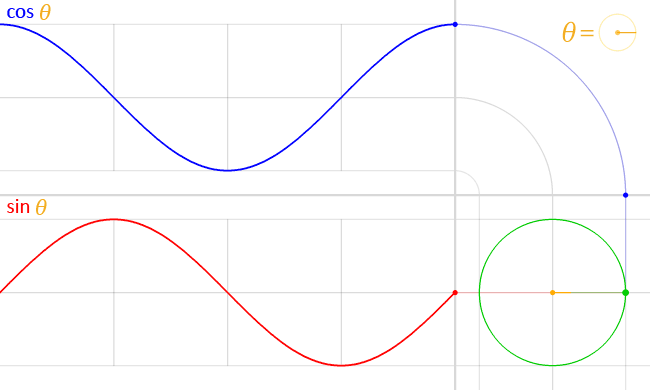
In the reference frame of the particle itself, the geometry of the wavefunction simplifies to what is illustrated below: an oscillation in two dimensions which, viewed together, form a plane that would be perpendicular to the direction of motion—but then our particle doesn’t move in its own reference frame, obviously. Hence, we could be looking at our particle from any direction and we should, presumably, see a similar two-dimensional oscillation. That is interesting because… Well… If we rotate this circle around its center (in whatever direction we’d choose), we get a sphere, right? It’s only when it starts moving, that it loses its symmetry. Now, that is very intriguing, but let’s think about that later.

Circle_cos_sin

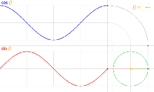
Let’s assume we’re looking at it from some specific direction. Then we presumably have some charge (the green dot) moving about some center, and its movement can be analyzed as the sum of two oscillations (the sine and cosine) which represent the real and imaginary component of the wavefunction respectively—as we observe it, so to speak. [Of course, you’ve been told you can’t observe wavefunctions so… Well… You should probably stop reading this. :-)] We write:

ψ = = a·e^−i∙θ = a·e^{−i∙E·t/ħ} = a·cos(−E∙t/ħ) + i·a·sin(−E∙t/ħ) = a·cos(E∙t/ħ) − i·a·sin(E∙t/ħ)

So that’s the wavefunction in the reference frame of the particle itself. When we think of it as moving in some direction (so relativity kicks in), we need to add the p·x term to the argument (θ = E·t − p∙x). It is easy to show this term doesn’t change the argument (θ), because we also get a different value for the energy in the new reference frame: E_v= γ·E₀ and so… Well… I’ll refer you to my post on this, in which I show the argument of the wavefunction is invariant under a Lorentz transformation: the way E_v and p_v and, importantly, the coordinates x and t relativistically transform ensures the invariance.

In fact, I’ve always wanted to read de Broglie‘s original thesis because I strongly suspect he saw that immediately. If you click this link, you’ll find an author who suggests the same. Having said that, I should immediately add this does not imply there is no need for a relativistic wave equation: the wavefunction is a solution for the wave equation and, yes, I am the first to note the Schrödinger equation has some obvious issues, which I briefly touch upon in one of my other posts—and which is why Schrödinger himself and other contemporaries came up with a relativistic wave equation (Oskar Klein and Walter Gordon got the credit but others (including Louis de Broglie) also suggested a relativistic wave equation when Schrödinger published his). In my humble opinion, the key issue is not that Schrödinger’s equation is non-relativistic. It’s that 1/2 factor again but… Well… I won’t dwell on that here. We need to move on. So let’s leave the wave equation for what it is and go back to our wavefunction.

You’ll note the argument (or phase) of our wavefunction moves clockwise—or counterclockwise, depending on whether you’re standing in front of behind the clock. Of course, Nature doesn’t care about where we stand or—to put it differently—whether we measure time clockwise, counterclockwise, in the positive, the negative or whatever direction. Hence, I’ve argued we can have both left- as well as right-handed wavefunctions, as illustrated below (for p ≠ 0). Our hypothesis is that these two physical possibilities correspond to the angular momentum of our electron being either positive or negative: J_z = +ħ/2 or, else, J_z = −ħ/2. [If you’ve read a thing or two about neutrinos, then… Well… They’re kinda special in this regard: they have no charge and neutrinos and antineutrinos are actually defined by their helicity. But… Well… Let’s stick to trying to describing electrons for a while.]

The line of reasoning that we followed allowed us to calculate the amplitude a. We got a result that tentatively confirms we’re on the right track with our interpretation: we found that a = ħ/m_e·c, so that’s the Compton scattering radius of our electron. All good ! But we were still a bit stuck—or ambiguous, I should say—on what the components of our wavefunction actually are. Are we really imagining the tip of that rotating arrow is a pointlike electric charge spinning around the center? [Pointlike or… Well… Perhaps we should think of the Thomson radius of the electron here, i.e. the so-called classical electron radius, which is equal to the Compton radius times the fine-structure constant: r_Thomson = α·r_Compton ≈ 3.86×10⁻¹³/137.]

So that would be the flywheel model.

In contrast, we may also think the whole arrow is some rotating field vector—something like the electric field vector, with the same or some other physical dimension, like newton per charge unit, or newton per mass unit? So that’s the field model. Now, these interpretations may or may not be compatible—or complementary, I should say. I sure hope they are but… Well… What can we reasonably say about it?

Let us first note that the flywheel interpretation has a very obvious advantage, because it allows us to explain the interaction between a photon and an electron, as I demonstrated in my previous post: the electromagnetic energy of the photon will drive the circulatory motion of our electron… So… Well… That’s a nice physical explanation for the transfer of energy. However, when we think about interference or diffraction, we’re stuck: flywheels don’t interfere or diffract. Only waves do. So… Well… What to say?

I am not sure, but here I want to think some more by pushing the flywheel metaphor to its logical limits. Let me remind you of what triggered it all: it was the mathematical equivalence of the energy equation for an oscillator (E = m·a²·ω²) and Einstein’s formula (E = m·c²), which tells us energy and mass are equivalent but… Well… They’re not the same. So what are they then? What is energy, and what is mass—in the context of these matter-waves that we’re looking at. To be precise, the E = m·a²·ω² formula gives us the energy of two oscillators, so we need a two-spring model which—because I love motorbikes—I referred to as my V-twin engine model, but it’s not an engine, really: it’s two frictionless pistons (or springs) whose direction of motion is perpendicular to each other, so they are in a 90° degree angle and, therefore, their motion is, effectively, independent. In other words: they will not interfere with each other. It’s probably worth showing the illustration just one more time. And… Well… Yes. I’ll also briefly review the math one more time.

V-2 engine

If the magnitude of the oscillation is equal to a, then the motion of these piston (or the mass on a spring) will be described by x = a·cos(ω·t + Δ). Needless to say, Δ is just a phase factor which defines our t = 0 point, and ω is the natural angular frequency of our oscillator. Because of the 90° angle between the two cylinders, Δ would be 0 for one oscillator, and –π/2 for the other. Hence, the motion of one piston is given by x = a·cos(ω·t), while the motion of the other is given by x = a·cos(ω·t–π/2) = a·sin(ω·t). The kinetic and potential energy of one oscillator – think of one piston or one spring only – can then be calculated as:

K.E. = T = m·v²/2 = (1/2)·m·ω²·a²·sin²(ω·t + Δ)
P.E. = U = k·x²/2 = (1/2)·k·a²·cos²(ω·t + Δ)

The coefficient k in the potential energy formula characterizes the restoring force: F = −k·x. From the dynamics involved, it is obvious that k must be equal to m·ω². Hence, the total energy—for one piston, or one spring—is equal to:

E = T + U = (1/2)· m·ω²·a²·[sin²(ω·t + Δ) + cos²(ω·t + Δ)] = m·a²·ω²/2

Hence, adding the energy of the two oscillators, we have a perpetuum mobile storing an energy that is equal to twice this amount: E = m·a²·ω². It is a great metaphor. Somehow, in this beautiful interplay between linear and circular motion, energy is borrowed from one place and then returns to the other, cycle after cycle. However, we still have to prove this engine is, effectively, a perpetuum mobile: we need to prove the energy that is being borrowed or returned by one piston is the energy that is being returned or borrowed by the other. That is easy to do, but I won’t bother you with that proof here: you can double-check it in the referenced post or – more formally – in an article I posted on viXra.org.

It is all beautiful, and the key question is obvious: if we want to relate the E = m·a²·ω² and E = m·c² formulas, we need to explain why we could, potentially, write c as c = a·ω = a·√(k/m). We’ve done that already—to some extent at least. The tangential velocity of a pointlike particle spinning around some axis is given by v = r·ω. Now, the radius r is given by a = ħ/(m·c), and ω = E/ħ = m·c²/ħ, so v is equal to to v = [ħ/(m·c)]·[m·c²/ħ] = c. Another beautiful result, but what does it mean? We need to think about the meaning of the ω = √(k/m) formula here. In the mentioned article, we boldly wrote that the speed of light is to be interpreted as the resonant frequency of spacetime, but so… Well… What do we really mean by that? Think of the following.

Einstein’s E = mc² equation implies the ratio between the energy and the mass of any particle is always the same:

This effectively reminds us of the ω² = C^–¹/L or ω² = k/m formula for harmonic oscillators. The key difference is that the ω²= C^–¹/L and ω² = k/m formulas introduce two (or more) degrees of freedom. In contrast, c²= E/m for any particle, always. However, that is exactly the point: we can modulate the resistance, inductance and capacitance of electric circuits, and the stiffness of springs and the masses we put on them, but we live in one physical space only: our spacetime. Hence, the speed of light (c) emerges here as the defining property of spacetime: the resonant frequency, so to speak. We have no further degrees of freedom here.

Let’s think about k. [I am not trying to avoid the ω²= 1/LC formula here. It’s basically the same concept: the ω²= 1/LC formula gives us the natural or resonant frequency for a electric circuit consisting of a resistor, an inductor, and a capacitor. Writing the formula as ω²= C⁻¹/L introduces the concept of elastance, which is the equivalent of the mechanical stiffness (k) of a spring, so… Well… You get it, right? The ω²= C^–¹/L and ω² = k/m sort of describe the same thing: harmonic oscillation. It’s just… Well… Unlike the ω²= C^–¹/L, the ω² = k/m is directly compatible with our V-twin engine metaphor, because it also involves physical distances, as I’ll show you here.] The k in the ω² = k/m is, effectively, the stiffness of the spring. It is defined by Hooke’s Law, which states that the force that is needed to extend or compress a spring by some distance x is linearly proportional to that distance, so we write: F = k·x.

Now that is interesting, isn’t it? We’re talking exactly the same thing here: spacetime is, presumably, isotropic, so it should oscillate the same in any direction—I am talking those sine and cosine oscillations now, but in physical space—so there is nothing imaginary here: all is real or… Well… As real as we can imagine it to be. 🙂

We can elaborate the point as follows. The F = k·x equation implies k is a force per unit distance: k = F/x. Hence, its physical dimension is newton per meter (N/m). Now, the x in this equation may be equated to the maximum extension of our spring, or the amplitude of the oscillation, so that’s the radius r = a in the metaphor we’re analyzing here. Now look at how we can re-write the c = a·ω = a·√(k/m) equation:

Einstein

In case you wonder about the E = F·a substitution: just remember that energy is force times distance. [Just do a dimensional analysis: you’ll see it works out.] So we have a spectacular result here, for several reasons. The first, and perhaps most obvious reason, is that we can actually derive Einstein’s E = m·c² formula from our flywheel model. Now, that is truly glorious, I think. However, even more importantly, this equation suggests we do not necessarily need to think of some actual mass oscillating up and down and sideways at the same time: the energy in the oscillation can be thought of a force acting over some distance, regardless of whether or not it is actually acting on a particle. Now, that energy will have an equivalent mass which is—or should be, I’d say… Well… The mass of our electron or, generalizing, the mass of the particle we’re looking at.

Huh? Yes. In case you wonder what I am trying to get at, I am trying to convey the idea that the two interpretations—the field versus the flywheel model—are actually fully equivalent, or compatible, if you prefer that term. In Asia, they would say: they are the “same-same but different” 🙂 but, using the language that’s used when discussing the Copenhagen interpretation of quantum physics, we should actually say the two models are complementary.

You may shrug your shoulders but… Well… It is a very deep philosophical point, really. 🙂 As far as I am concerned, I’ve never seen a better illustration of the (in)famous Complementarity Principle in quantum physics because… Well… It goes much beyond complementarity. This is about equivalence. 🙂 So it’s just like Einstein’s equation. 🙂

Post scriptum: If you read my posts carefully, you’ll remember I struggle with those 1/2 factors here and there. Textbooks don’t care about them. For example, when deriving the size of an atom, or the Rydberg energy, even Feynman casually writes that “we need not trust our answer [to questions like this] within factors like 2, π, etcetera.” Frankly, that’s disappointing. Factors like 2, 1/2, π or 2π are pretty fundamental numbers, and so they need an explanation. So… Well… I do loose sleep over them. Let me advance some possible explanation here.

As for Feynman’s model, and the derivation of electron orbitals in general, I think it’s got to do with the fact that electrons do want to pair up when thermal motion does not come into play: think of the Cooper pairs we use to explain superconductivity (so that’s the BCS theory). The 1/2 factor in Schrödinger’s equation also has weird consequences (when you plug in the elementary wavefunction and do the derivatives, you get a weird energy concept: E = m·v², to be precise). This problem may also be solved when assuming we’re actually calculating orbitals for a pair of electrons, rather than orbitals for just one electron only. [We’d get twice the mass (and, presumably, the charge, so… Well… It might work—but I haven’t done it yet. It’s on my agenda—as so many other things, but I’ll get there… One day. :-)]

So… Well… Let’s get back to the lesson here. In this particular context (i.e. in the context of trying to find some reasonable physical interpretation of the wavefunction), you may or may not remember (if not, check my post on it) ‘ll remember I had to use the I = m·r²/2 formula for the angular momentum, as opposed to the I = m·r² formula. I = m·r²/2 (with the 1/2 factor) gives us the angular momentum of a disk with radius r, as opposed to a point mass going around some circle with radius r. I noted that “the addition of this 1/2 factor may seem arbitrary”—and it totally is, of course—but so it gave us the result we wanted: the exact (Compton scattering) radius of our electron.

Now, the arbitrary 1/2 factor may or may be explained as follows. In the field model of our electron, the force is linearly proportional to the extension or compression. Hence, to calculate the energy involved in stretching it from x = 0 to x = a, we need to calculate it as the following integral:

So… Well… That will give you some food for thought, I’d guess. 🙂 If it racks your brain too much—or if you’re too exhausted by this point (which is OK, because it racks my brain too!)—just note we’ve also shown that the energy is proportional to the square of the amplitude here, so that’s a nice result as well… 🙂

Talking food for thought, let me make one final point here. The c² = a²·k/m relation implies a value for k which is equal to k = m·c²/a = E/a. What does this tell us? In one of our previous posts, we wrote that the radius of our electron appeared as a natural distance unit. We wrote that because of another reason: the remark was triggered by the fact that we can write the c/ω ratio as c/ω = a·ω/ω = a. This implies the tangential and angular velocity in our flywheel model of an electron would be the same if we’d measure distance in units of a. Now, the E = a·k = a·F/x (just re-writing…) implies that the force is proportional to the energy— F = (x/a)·E — and the proportionality coefficient is… Well… x/a. So that’s the distance measured in units of a. So… Well… Isn’t that great? The radius of our atom appearing as a natural distance unit does fit in nicely with our geometric interpretation of the wavefunction, doesn’t it? I mean… Do I need to say more?

I hope not because… Well… I can’t explain any better for the time being. I hope I sort of managed to convey the message. Just to make sure, in case you wonder what I was trying to do here, it’s the following: I told you c appears as a resonant frequency of spacetime and, in this post, I tried to explain what that really means. I’d appreciate if you could let me know if you got it. If not, I’ll try again. 🙂 When everything is said and done, one only truly understands stuff when one is able to explain it to someone else, right? 🙂 Please do think of more innovative or creative ways if you can! 🙂

OK. That’s it but… Well… I should, perhaps, talk about one other thing here. It’s what I mentioned in the beginning of this post: this analysis assumes we’re looking at our particle from some specific direction. It could be any direction but… Well… It’s some direction. We have no depth in our line of sight, so to speak. That’s really interesting, and I should do some more thinking about it. Because the direction could be any direction, our analysis is valid for any direction. Hence, if our interpretation would happen to be some true—and that’s a big if, of course—then our particle has to be spherical, right? Why? Well… Because we see this circular thing from any direction, so it has to be a sphere, right?

Well… Yes. But then… Well… While that logic seems to be incontournable, as they say in French, I am somewhat reluctant to accept it at face value. Why? I am not sure. Something inside of me says I should look at the symmetries involved… I mean the transformation formulas for wavefunction when doing rotations and stuff. So… Well… I’ll be busy with that for a while, I guess. 😦

Post scriptum 2: You may wonder whether this line of reasoning would also work for a proton. Well… Let’s try it. Because its mass is so much larger than that of an electron (about 1835 times), the a = ħ/(m·c) formula gives a much smaller radius: 1835 times smaller, to be precise, so that’s around 2.1×10⁻¹⁶ m, which is about 1/4 of the so-called charge radius of a proton, as measured by scattering experiments. So… Well… We’re not that far off, but… Well… We clearly need some more theory here. Having said that, a proton is not an elementary particle, so its mass incorporates other factors than what we’re considering here (two-dimensional oscillations).

The Complementarity Principle

Pre-script (dated 26 June 2020): This post has become less relevant because my views on all things quantum-mechanical have evolved significantly as a result of my progression towards a more complete realist (classical) interpretation of quantum physics. Hence, we recommend you read our recent papers. I keep blog posts like these mainly because I want to keep track of where I came from. I might review them one day, but I currently don’t have the time or energy for it. 🙂

Original post:

Unlike what you might think when seeing the title of this post, it is not my intention to enter into philosophical discussions here: many authors have been writing about this ‘principle’, most of which–according to eminent physicists–don’t know what they are talking about. So I have no intention to make a fool of myself here too. However, what I do want to do here is explore, in an intuitive way, how the classical and quantum-mechanical explanations of the phenomenon of the diffraction of light are different from each other–and fundamentally so–while, necessarily, having to yield the same predictions. It is in that sense that the two explanations should be ‘complementary’.

The classical explanation

I’ve done a fairly complete analysis of the classical explanation in my posts on Diffraction and the Uncertainty Principle (20 and 21 September), so I won’t dwell on that here. Let me just repeat the basics. The model is based on the so-called Huygens-Fresnel Principle, according to which each point in the slit becomes a source of a secondary spherical wave. These waves then interfere, constructively or destructively, and, hence, by adding them, we get the form of the wave at each point of time and at each point in space behind the slit. The animation below illustrates the idea. However, note that the mathematical analysis does not assume that the point sources are neatly separated from each other: instead of only six point sources, we have an infinite number of them and, hence, adding up the waves amounts to solving some integral (which, as you know, is an infinite sum).

We know what we are supposed to get: a diffraction pattern. The intensity of the light on the screen at the other side depends on (1) the slit width (d), (2) the frequency of the light (λ), and (3) the angle of incidence (θ), as shown below.

$Single_Slit_Diffraction_(english)$

One point to note is that we have smaller bumps left and right. We don’t get that if we’d treat the slit as a single point source only, like Feynman does when he discusses the double-slit experiment for (physical) waves. Indeed, look at the image below: each of the slits acts as one point source only and, hence, the intensity curves I₁and I₂ do not show a diffraction pattern. They are just nice Gaussian “bell” curves, albeit somewhat adjusted because of the angle of incidence (we have two slits above and below the center, instead of just one on the normal itself). So we have an interference pattern on the screen and, now that we’re here, let me be clear on terminology: I am going along with the widespread definition of diffraction being a pattern created by one slit, and the definition of interference as a pattern created by two or more slits. I am noting this just to make sure there’s no confusion.

That should be clear enough. Let’s move on the quantum-mechanical explanation.

The quantum-mechanical explanation

There are several formulations of quantum mechanics: you’ve heard about matrix mechanics and wave mechanics. Roughly speaking, in matrix mechanics “we interpret the physical properties of particles as matrices that evolve in time”, while the wave mechanics approach is primarily based on these complex-valued wave functions–one for each physical property (e.g. position, momentum, energy). Both approaches are mathematically equivalent.

There is also a third approach, which is referred to as the path integral formulation, which “replaces the classical notion of a single, unique trajectory for a system with a sum, or functional integral, over an infinity of possible trajectories to compute an amplitude” (all definitions here were taken from Wikipedia). This approach is associated with Richard Feynman but can also be traced back to Paul Dirac, like most of the math involved in quantum mechanics, it seems. It’s this approach which I’ll try to explain–again, in an intuitive way only–in order to show the two explanations should effectively lead to the same predictions.

The key to understanding the path integral formulation is the assumption that a particle–and a ‘particle’ may refer to both bosons (e.g. photons) or fermions (e.g. electrons)–can follow any path from point A to B, as illustrated below. Each of these paths is associated with a (complex-valued) probability amplitude, and we have to add all these probability amplitudes to arrive at the probability amplitude for the particle to move from A to B.

You can find great animations illustrating what it’s all about in the relevant Wikipedia article but, because I can’t upload video here, I’ll just insert two illustrations from Feynman’s 1985 QED, in which he does what I try to do, and that is to approach the topic intuitively, i.e. without too much mathematical formalism. So probability amplitudes are just ‘arrows’ (with a length and a direction, just like a complex number or a vector), and finding the resultant or final arrow is a matter of just adding all the little arrows to arrive at one big arrow, which is the probability amplitude, which he denotes as P(A, B), as shown below.

This intuitive approach is great and actually goes a very long way in explaining complicated phenomena, such as iridescence for example (the wonderful patterns of color on an oil film!), or the partial reflection of light by glass (anything between 0 and 16%!). All his tricks make sense. For example, different frequencies are interpreted as slower or faster ‘stopwatches’ and, as such, they determine the final direction of the arrows which, in turn, explains why blue and red light are reflected differently. And so on and son. It all works. […] Up to a point.

Indeed, Feynman does get in trouble when trying to explain diffraction. I’ve reproduced his explanation below. The key to the argument is the following:

If we have a slit that’s very wide, there are a lot of possible paths for the photon to take. However, most of these paths cancel each other out, and so that’s why the photon is likely to travel in a straight line. Let me quote Feynman: “When the gap between the blocks is wide enough to allow many neighboring paths to P and Q, the arrows for the paths to P add up (because all the paths to P take nearly the same time), while the paths to Q cancel out (because those paths have a sizable difference in time). So the photomultiplier at Q doesn’t click.” (QED, p.54)
However, “when the gap is nearly closed and there are only a few neighboring paths, the arrows to Q also add up, because there is hardly any difference in time between them, either (see Fig. 34). Of course, both final arrows are small, so there’s not much light either way through such a small hole, but the detector at Q clicks almost as much as the one at P! So when you try to squeeze light too much to make sure it’s going only in a straight line, it refuses to cooperate and begins to spread out.” (QED, p. 55)

This explanation is as simple and intuitive as Feynman’s ‘explanation’ of diffraction using the Uncertainty Principle in his introductory chapter on quantum mechanics (Lectures, I-38-2), which is illustrated below. I won’t go into the detail (I’ve done that before) but you should note that, just like the explanation above, such explanations do not explain the secondary, tertiary etc bumps in the diffraction pattern.

$Diffraction of electrons$

So what’s wrong with these explanations? Nothing much. They’re simple and intuitive, but essentially incomplete, because they do not incorporate all of the math involved in interference. Incorporating the math means doing these integrals for

Electromagnetic waves in classical mechanics: here we are talking ‘wave functions’ with some real-valued amplitude representing the strength of the electric and magnetic field; and
Probability waves: these are complex-valued functions, with the complex-valued amplitude representing probability amplitudes.

The two should, obviously, yield the same result, but a detailed comparison between the approaches is quite complicated, it seems. Now, I’ve googled a lot of stuff, and I duly note that diffraction of electromagnetic waves (i.e. light) is conveniently analyzed by summing up complex-valued waves too, and, moreover, they’re of the same familiar type: ψ = Ae^i(kx–ωt). However, these analyses also duly note that it’s only the real part of the wave that has an actual physical interpretation, and that it’s only because working with natural exponentials (addition, multiplication, integration, derivation, etc) is much easier than working with sine and cosine waves that such complex-valued wave functions are used (also) in classical mechanics. In fact, note the fine print in Feynman’s illustration of interference of physical waves (Fig. 37-2): he calculates the intensities I₁and I₂ by taking the square of the absolute amplitudes ĥ₁ and ĥ₂, and the hat indicates that we’re also talking some complex-valued wave function here.

Hence, we must be talking the same mathematical waves in both explanations, aren’t we? In other words, we should get the same psi functions ψ = Ae^i(kx–ωt) in both explanations, don’t we? Well… Maybe. But… Probably not. As far as I know–but I must be wrong–we cannot just re-normalize the E and B vectors in these electromagnetic waves in order to establish an equivalence with probability waves. I haven’t seen that being done (but I readily admit I still have a lot of reading to do) and so I must assume it’s not very clear-cut at all.

So what? Well… I don’t know. So far, I did not find a ‘nice’ or ‘intuitive’ explanation of a quantum-mechanical approach to the phenomenon of diffraction yielding the same grand diffraction equation, referred to as the Fresnel-Kirchoff diffraction formula (see below), or one of its more comprehensible (because simplified) representations, such as the Fraunhofer diffraction formula, or the even easier formula which I used in my own post (you can google them: they’re somewhat less monstrous and–importantly–they work with real numbers only, which makes them easier to understand).

[…] That looks pretty daunting, isn’t it? You may start to understand it a bit better by noting that (n, r) and (n, s) are angles, so that’s OK in a cosine function. The other variables also have fairly standard interpretations, as shown below, but… Admit it: ‘easy’ is something else, isn’t it?

So… Where are we here? Well… As said, I trust that both explanations are mathematically equivalent – just like matrix and wave mechanics 🙂 –and, hence, that a quantum-mechanical analysis will indeed yield the same formula. However, I think I’ll only understand physics truly if I’ve gone through all of the motions here.

Well then… I guess that should be some kind of personal benchmark that should guide me on this journey, isn’t it? 🙂 I’ll keep you posted.

Post scriptum: To be fair to Feynman, and demonstrating his talent as a teacher once again, he actually acknowledges that the double-slit thought experiment uses simplified assumptions that do not include diffraction effects when the electrons go through the slit(s). He does so, however, only in one of the first chapters of Vol. III of the Lectures, where he comes back to the experiment to further discuss the first principles of quantum mechanics. I’ll just quote him: “Incidentally, we are going to suppose that the holes 1 and 2 are small enough that when we say an electron goes through the hole, we don’t have to discuss which part of the hole. We could, of course, split each hole into pieces with a certain amplitude that the electron goes to the top of the hole and the bottom of the hole and so on. We will suppose that the hole is small enough so that we don’t have to worry about this detail. That is part of the roughness involved; the matter can be made more precise, but we don’t want to do so at this stage.” So here he acknowledges that he omitted the intricacies of diffraction. I noted this only later. Sorry.

Some content on this page was disabled on June 17, 2020 as a result of a DMCA takedown notice from Michael A. Gottlieb, Rudolf Pfeiffer, and The California Institute of Technology. You can learn more about the DMCA here:

https://en.support.wordpress.com/copyright-and-the-dmca/
Some content on this page was disabled on June 20, 2020 as a result of a DMCA takedown notice from Michael A. Gottlieb, Rudolf Pfeiffer, and The California Institute of Technology. You can learn more about the DMCA here:

https://en.support.wordpress.com/copyright-and-the-dmca/