Transforming amplitudes for spin-1/2 particles

Pre-script (dated 26 June 2020): This post got mutilated by the removal of some material by the dark force. You should be able to follow the main story line, however. If anything, the lack of illustrations might actually help you to think things through for yourself. In any case, we now have different views on these concepts as part of our realist interpretation of quantum mechanics, so we recommend you read our recent papers instead of these old blog posts.

Original post:

Some say it is not possible to fully understand quantum-mechanical spin. Now, I do agree it is difficult, but I do not believe it is impossible. That’s why I wrote so many posts on it. Most of these focused on elaborating how the classical view of how a rotating charge precesses in a magnetic field might translate into the weird world of quantum mechanics. Others were more focused on the corollary of the quantization of the angular momentum, which is that, in the quantum-mechanical world, the angular momentum is never quite all in one direction only—so that explains some of the seemingly inexplicable randomness in particle behavior.

Frankly, I think those explanations help us quite a bit already but… Well… We need to go the extra mile, right? In fact, that’s drives my search for a geometric (or physical) interpretation of the wavefunction: the extra mile. 🙂

Now, in one of these many posts on spin and angular momentum, I advise my readers – you, that is – to try to work yourself through Feynman’s 6th Lecture on quantum mechanics, which is highly abstract and, therefore, usually skipped. [Feynman himself told his students to skip it, so I am sure that’s what they did.] However, if we believe the physical (or geometric) interpretation of the wavefunction that we presented in previous posts is, somehow, true, then we need to relate it to the abstract math of these so-called transformations between representations. That’s what we’re going to try to do here. It’s going to be just a start, and I will probably end up doing several posts on this but… Well… We do have to start somewhere, right? So let’s see where we get today. 🙂

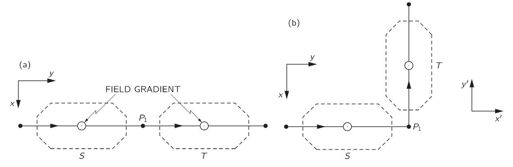
The thought experiment that Feynman uses throughout his Lecture makes use of what Feynman’s refers to as modified or improved Stern-Gerlach apparatuses. They allow us to prepare a pure state or, alternatively, as Feynman puts it, to analyze a state. In theory, that is. The illustration below present a side and top view of such apparatus. We may already note that the apparatus itself—or, to be precise, our perspective of it—gives us two directions: (1) the up direction, so that’s the positive direction of the z-axis, and (2) the direction of travel of our particle, which coincides with the positive direction of the y-axis. [This is obvious and, at the same time, not so obvious, but I’ll talk about that in my next post. In this one, we basically need to work ourselves through the math, so we don’t want to think too much about philosophical stuff.]

Modified Stern-Gerlach

The kind of questions we want to answer in this post are variants of the following basic one: if a spin-1/2 particle (let’s think of an electron here, even if the Stern-Gerlach experiment is usually done with an atomic beam) was prepared in a given condition by one apparatus S, say the +S state, what is the probability (or the amplitude) that it will get through a second apparatus T if that was set to filter out the +T state?

The result will, of course, depend on the angles between the two apparatuses S and T, as illustrated below. [Just to respect copyright, I should explicitly note here that all illustrations are taken from the mentioned Lecture, and that the line of reasoning sticks close to Feynman’s treatment of the matter too.]

basic set-up

We should make a few remarks here. First, this thought experiment assumes our particle doesn’t get lost. That’s obvious but… Well… If you haven’t thought about this possibility, I suspect you will at some point in time. So we do assume that, somehow, this particle makes a turn. It’s an important point because… Well… Feynman’s argument—who, remember, represents mainstream physics—somehow assumes that doesn’t really matter. It’s the same particle, right? It just took a turn, so it’s going in some other direction. That’s all, right? Hmm… That’s where I part ways with mainstream physics: the transformation matrices for the amplitudes that we’ll find here describe something real, I think. It’s not just perspective: something happened to the electron. That something does not only change the amplitudes but… Well… It describes a different electron. It describes an electron that goes in a different direction now. But… Well… As said, these are reflections I will further develop in my next post. 🙂 Let’s focus on the math here. The philosophy will follow later. 🙂 Next remark.

Second, we assume the (a) and (b) illustrations above represent the same physical reality because the relative orientation between the two apparatuses, as measured by the angle α, is the same. Now that is obvious, you’ll say, but, as Feynman notes, we can only make that assumption because experiments effectively confirm that spacetime is, effectively, isotropic. In other words, there is no aether allowing us to establish some sense of absolute direction. Directions are relative—relative to the observer, that is… But… Well… Again, in my next post, I’ll argue that it’s not because directions are relative that they are, somehow, not real. Indeed, in my humble opinion, it does matter whether an electron goes here or, alternatively, there. These two different directions are not just two different coordinate frames. But… Well… Again. The philosophy will follow later. We need to stay focused on the math here.

Third and final remark. This one is actually very tricky. In his argument, Feynman also assumes the two set-ups below are, somehow, equivalent.

equivalent set-up

You’ll say: Huh? If not, say it! Huh? 🙂 Yes. Good. Huh? Feynman writes equivalent—not the same because… Well… They’re not the same, obviously:

In the first set-up (a), T is wide open, so the apparatus is not supposed to do anything with the beam: it just splits and re-combines it.
In set-up (b) the T apparatus is, quite simply, not there, so… Well… Again. Nothing is supposed to happen with our particles as they come out of S and travel to U.

The fundamental idea here is that our spin-1/2 particle (again, think of an electron here) enters apparatus U in the same state as it left apparatus S. In both set-ups, that is! Now that is a very tricky assumption, because… Well… While the net turn of our electron is the same, it is quite obvious it has to take two turns to get to U in (a), while it only takes one turn in (b). And so… Well… You can probably think of other differences too. So… Yes. And no. Same-same but different, right? 🙂

Right. That is why Feynman goes out of his way to explain the nitty-gritty behind: he actually devotes a full page in small print on this, which I’ll try to summarize in just a few paragraphs here. [And, yes, you should check my summary against Feynman’s actual writing on this.] It’s like this. While traveling through apparatus T in set-up (a), time goes by and, therefore, the amplitude would be different by some phase factor δ. [Feynman doesn’t say anything about this, but… Well… In the particle’s own frame of reference, this phase factor depend on the energy, the momentum and the time and distance traveled. Think of the argument of the elementary wavefunction here: θ = (E∙t – p∙x)/ħ).] Now, if we believe that the amplitude is just some mathematical construct—so that’s what mainstream physicists (not me!) believe—then we could effectively say that the physics of (a) and (b) are the same, as Feynman does. In fact, let me quote him here:

“The physics of set-up (a) and (b) should be the same but the amplitudes could be different by some phase factor without changing the result of any calculation about the real world.”

Hmm… It’s one of those mysterious short passages where we’d all like geniuses like Feynman (or Einstein, or whomever) to be more explicit on their world view: if the amplitudes are different, can the physics really be the same? I mean… Exactly the same? It all boils down to that unfathomable belief that, somehow, the particle is real but the wavefunction that describes it, is not. Of course, I admit that it’s true that choosing another zero point for the time variable would also change all amplitudes by a common phase factor and… Well… That’s something that I consider to be not real. But… Well… The time and distance traveled in the T apparatus is the time and distance traveled in the T apparatus, right?

Bon… I have to stay away from these questions as for now—we need to move on with the math here—but I will come back to it later. But… Well… Talking math, I should note a very interesting mathematical point here. We have these transformation matrices for amplitudes, right? Well… Not yet. In fact, the coefficient of these matrices are exactly what we’re going to try to derive in this post, but… Well… Let’s assume we know them already. 🙂 So we have a 2-by-2 matrix to go from S to T, from T to U, and then one to go from S to U without going through T, which we can write as R^ST, R^TU, and R^SU respectively. Adding the subscripts for the base states in each representation, the equivalence between the (a) and (b) situations can then be captured by the following formula:

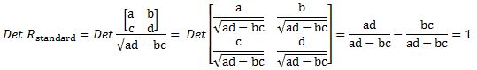
So we have that phase factor here: the left- and right-hand side of this equation is, effectively, same-same but different, as they would say in Asia. 🙂 Now, Feynman develops a beautiful mathematical argument to show that the eⁱ^δ factor effectively disappears if we convert our rotation matrices to some rather special form that is defined as follows:

I won’t copy his argument here, but I’d recommend you go over it because it is wonderfully easy to follow and very intriguing at the same time. [Yes. Simple things can be very intriguing.] Indeed, the calculation below shows that the determinant of these special rotation matrices will be equal to 1.

det is one

So… Well… So what? You’re right. I am being sidetracked here. The point is that, if we put all of our rotation matrices in this special form, the eⁱ^δ factor vanishes and the formula above reduces to:

So… Yes. End of excursion. Let us remind ourselves of what it is that we are trying to do here. As mentioned above, the kind of questions we want to answer will be variants of the following basic one: if a spin-1/2 particle was prepared in a given condition by one apparatus (S), say the +S state, what is the probability (or the amplitude) that it will get through a second apparatus (T) if that was set to filter out the +T state?

We said the result would depend on the angles between the two apparatuses S and T. I wrote: angles—plural. Why? Because a rotation will generally be described by the three so-called Euler angles: α, β and γ. Now, it is easy to make a mistake here, because there is a sequence to these so-called elemental rotations—and right-hand rules, of course—but I will let you figure that out. 🙂

The basic idea is the following: if we can work out the transformation matrices for each of these elemental rotations, then we can combine them and find the transformation matrix for any rotation. So… Well… That fills most of Feynman’s Lecture on this, so we don’t want to copy all that. We’ll limit ourselves to the logic for a rotation about the z-axis, and then… Well… You’ll see. 🙂

So… The z-axis… We take that to be the direction along which we are measuring the angular momentum of our electron, so that’s the direction of the (magnetic) field gradient, so that’s the up-axis of the apparatus. In the illustration below, that direction points out of the page, so to speak, because it is perpendicular to the direction of the x– and the y-axis that are shown. Note that the y-axis is the initial direction of our beam.

rotation about z

Now, because the (physical) orientation of the fields and the field gradients of S and T is the same, Feynman says that—despite the angle—the probability for a particle to be up or down with regard to S and T respectively should be the same. Well… Let’s be fair. He does not only say that: experiment shows it to be true. [Again, I am tempted to interject here that it is not because the probabilities for (a) and (b) are the same, that the reality of (a) and (b) is the same, but… Well… You get me. That’s for the next post. Let’s get back to the lesson here.] The probability is, of course, the square of the absolute value of the amplitude, which we will denote as C₊, C₋, C’₊, and C’₋ respectively. Hence, we can write the following:

Now, the absolute values (or the magnitudes) are the same, but the amplitudes may differ. In fact, they must be different by some phase factor because, otherwise, we would not be able to distinguish the two situations, which are obviously different. As Feynman, finally, admits himself—jokingly or seriously: “There must be some way for a particle to know that it has turned the corner at P₁.” [P₁ is the midway point between S and T in the illustration, of course—not some probability.]

So… Well… We write:

C’₊ = eⁱ^λ ·C₊ and C’₋ = eⁱ^μ ·C₋

Now, Feynman notes that an equal phase change in all amplitudes has no physical consequence (think of re-defining our t 0 = 0 point), so we can add some arbitrary amount to both λ and μ without changing any of the physics . So then we can choose this amount as -(λ + μ)/2. We write:

Now, it shouldn’t you too long to figure out that λ’ is equal to λ’ = λ/2 + μ/2 = −μ’. So… Well… Then we can just adopt the convention that λ = −μ. So our C’₊ = eⁱ^λ ·C₊ and C’₋ = eⁱ^μ ·C₋ equations can now be written as:

C’₊ = eⁱ^λ ·C₊ and C’₋ = e^−iλ·C₋

The absolute values are the same, but the phases are different. Right. OK. Good move. What’s next?

Well… The next assumption is that the phase shift λ is proportional to the angle (α) between the two apparatuses. Hence, λ is equal to λ = m·α, and we can re-write the above as:

C’₊ = eⁱ^mα·C₊ and C’₋ = e^−imα·C₋

Now, this assumption may or may not seem reasonable. Feynman justifies it with a continuity argument, arguing any rotation can be built up as a sequence of infinitesimal rotations and… Well… Let’s not get into the nitty-gritty here. [If you want it, check Feynman’s Lecture itself.] Back to the main line of reasoning. So we’ll assume we can write λ as λ = m·α. The next question then is: what is the value for m? Now, we obviously do get exactly the same physics if we rotate T by 360°, or 2π radians. So we might conclude that the amplitudes should be the same and, therefore, that eⁱ^mα = eⁱ^m·2π has to be equal to one, so C’₊ = C₊ and C’₋ = C₋ . That’s the case if m is equal to 1. But… Well… No. It’s the same thing again: the probabilities (or the magnitudes) have to be the same, but the amplitudes may be different because of some phase factor. In fact, they should be different. If m = 1/2, then we also get the same physics, even if the amplitudes are not the same. They will be each other’s opposite:

same physical state

Huh? Yes. Think of it. The coefficient of proportionality (m) cannot be equal to 1. If it would be equal to 1, and we’d rotate T by 180° only, then we’d also get those C’₊ = −C₊ and C’₋ = −C₋ equations, and so these coefficients would, therefore, also describe the same physical situation. Now, you will understand, intuitively, that a rotation of the T apparatus by 180° will not give us the same physical situation… So… Well… In case you’d want a more formal argument proving a rotation by 180° does not give us the same physical situation, Feynman has one for you. 🙂

I know that, by now, you’re totally tired and bored, and so you only want the grand conclusion at this point. Well… All of what I wrote above should, hopefully, help you to understand that conclusion, which – I quote Feynman here – is the following:

If we know the amplitudes C₊ and C₋ of spin one-half particles with respect to a reference frame S, and we then use new base states, defined with respect to a reference frame T which is obtained from S by a rotation α around the z-axis, the new amplitudes are given in terms of the old by the following formulas:

conclusion

[Feynman denotes our angle α by phi (φ) because… He uses the Euler angles a bit differently. But don’t worry: it’s the same angle.]

What about the amplitude to go from the C₋ to the C’₊ state, and from the C₊ to the C’₋ state? Well… That amplitude is zero. So the transformation matrix is this one:

rotation matrix

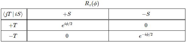
Let’s take a moment and think about this. Feynman notes the following, among other things: “It is very curious to say that if you turn the apparatus 360° you get new amplitudes. [They aren’t really new, though, because the common change of sign doesn’t give any different physics.] But if something has been rotated by a sequence of small rotations whose net result is to return it to the original orientation, then it is possible to define the idea that it has been rotated 360°—as distinct from zero net rotation—if you have kept track of the whole history.”

This is very deep. It connects space and time into one single geometric space, so to speak. But… Well… I’ll try to explain this rather sweeping statement later. Feynman also notes that a net rotation of 720° does give us the same amplitudes and, therefore, cannot be distinguished from the original orientation. Feynman finds that intriguing but… Well… I am not sure if it’s very significant. I do note some symmetries in quantum physics involve 720° rotations but… Well… I’ll let you think about this. 🙂

Note that the determinant of our matrix is equal to a·d − b·c = eⁱ^φ/2·e⁻ⁱ^φ/2 = 1. So… Well… Our rotation matrix is, effectively, in that special form! How comes? Well… When equating λ = −μ, we are effectively putting the transformation into that special form. Let us also, just for fun, quickly check the normalization condition. It requires that the probabilities, in any given representation, add to up to one. So… Well… Do they? When they come out of S, our electrons are equally likely to be in the up or down state. So the amplitudes are 1/√2. [To be precise, they are ±1/√2 but… Well… It’s the phase factor story once again.] That’s normalized: |1/√2|² + |1/√2|² = 1. The amplitudes to come out of the T apparatus in the up or down state are eⁱ^φ/2/√2 and eⁱ^φ/2/√2 respectively, so the probabilities add up to |eⁱ^φ/2/√2|² + |e⁻ⁱ^φ/2/√2|² = … Well… It’s 1. Check it. 🙂

Let me add an extra remark here. The normalization condition will result in matrices whose determinant will be equal to some pure imaginary exponential, like eⁱ^α. So is that what we have here? Yes. We can re-write 1 as 1 = eⁱ^·0 = e⁰, so α = 0. 🙂 Capito? Probably not, but… Well… Don’t worry about it. Just think about the grand results. As Feynman puts it, this Lecture is really “a sort of cultural excursion.” 🙂

Let’s do a practical calculation here. Let’s suppose the angle is, effectively, 180°. So the eⁱ^φ/2 and e⁻ⁱ^φ/2/√2 factors are equal to eⁱ^π/2 = +i and e⁻ⁱ^π/2 = −i, so… Well… What does that mean—in terms of the geometry of the wavefunction? Hmm… We need to do some more thinking about the implications of all this transformation business for our geometric interpretation of he wavefunction, but so we’ll do that in our next post. Let us first work our way out of this rather hellish transformation logic. 🙂 [See? I do admit it is all quite difficult and abstruse, but… Well… We can do this, right?]

So what’s next? Well… Feynman develops a similar argument (I should say same-same but different once more) to derive the coefficients for a rotation of ±90° around the y-axis. Why 90° only? Well… Let me quote Feynman here, as I can’t sum it up more succinctly than he does: “With just two transformations—90° about the y-axis, and an arbitrary angle about the z-axis [which we described above]—we can generate any rotation at all.”

So how does that work? Check the illustration below. In Feynman’s words again: “Suppose that we want the angle α around x. We know how to deal with the angle α α around z, but now we want it around x. How do we get it? First, we turn the axis z down onto x—which is a rotation of +90°. Then we turn through the angle α around x = . Then we rotate −90° about y”. The net result of the three rotations is the same as turning around x by the angle α. It is a property of space.”

full rotation

Besides helping us greatly to derive the transformation matrix for any rotation, the mentioned property of space is rather mysterious and deep. It sort of reduces the degrees of freedom, so to speak. Feynman writes the following about this:

“These facts of the combinations of rotations, and what they produce, are hard to grasp intuitively. It is rather strange, because we live in three dimensions, but it is hard for us to appreciate what happens if we turn this way and then that way. Perhaps, if we were fish or birds and had a real appreciation of what happens when we turn somersaults in space, we could more easily appreciate such things.”

In any case, I should limit the number of philosophical interjections. If you go through the motions, then you’ll find the following elemental rotation matrices:

full set of rotation matrices

What about the determinants of the R_x(φ) and R_y(φ) matrices? They’re also equal to one, so… Yes. A pure imaginary exponential, right? 1 = eⁱ^·0 = e⁰. 🙂

What’s next? Well… We’re done. We can now combine the elemental transformations above in a more general format, using the standardized Euler angles. Again, just go through the motions. The Grand Result is:

euler transformatoin

Does it give us normalized amplitudes? It should, but it looks like our determinant is going to be a much more complicated complex exponential. 🙂 Hmm… Let’s take some time to mull over this. As promised, I’ll be back with more reflections in my next post.

Some content on this page was disabled on June 16, 2020 as a result of a DMCA takedown notice from The California Institute of Technology. You can learn more about the DMCA here:

https://en.support.wordpress.com/copyright-and-the-dmca/
Some content on this page was disabled on June 16, 2020 as a result of a DMCA takedown notice from The California Institute of Technology. You can learn more about the DMCA here:

https://en.support.wordpress.com/copyright-and-the-dmca/
Some content on this page was disabled on June 16, 2020 as a result of a DMCA takedown notice from The California Institute of Technology. You can learn more about the DMCA here:

https://en.support.wordpress.com/copyright-and-the-dmca/
Some content on this page was disabled on June 16, 2020 as a result of a DMCA takedown notice from The California Institute of Technology. You can learn more about the DMCA here:

https://en.support.wordpress.com/copyright-and-the-dmca/
Some content on this page was disabled on June 16, 2020 as a result of a DMCA takedown notice from The California Institute of Technology. You can learn more about the DMCA here:

https://en.support.wordpress.com/copyright-and-the-dmca/
Some content on this page was disabled on June 16, 2020 as a result of a DMCA takedown notice from The California Institute of Technology. You can learn more about the DMCA here:

https://en.support.wordpress.com/copyright-and-the-dmca/
Some content on this page was disabled on June 16, 2020 as a result of a DMCA takedown notice from The California Institute of Technology. You can learn more about the DMCA here:

https://en.support.wordpress.com/copyright-and-the-dmca/
Some content on this page was disabled on June 16, 2020 as a result of a DMCA takedown notice from The California Institute of Technology. You can learn more about the DMCA here:

https://en.support.wordpress.com/copyright-and-the-dmca/
Some content on this page was disabled on June 16, 2020 as a result of a DMCA takedown notice from The California Institute of Technology. You can learn more about the DMCA here:

https://en.support.wordpress.com/copyright-and-the-dmca/
Some content on this page was disabled on June 16, 2020 as a result of a DMCA takedown notice from The California Institute of Technology. You can learn more about the DMCA here:

https://en.support.wordpress.com/copyright-and-the-dmca/
Some content on this page was disabled on June 17, 2020 as a result of a DMCA takedown notice from Michael A. Gottlieb, Rudolf Pfeiffer, and The California Institute of Technology. You can learn more about the DMCA here:

https://en.support.wordpress.com/copyright-and-the-dmca/
Some content on this page was disabled on June 17, 2020 as a result of a DMCA takedown notice from Michael A. Gottlieb, Rudolf Pfeiffer, and The California Institute of Technology. You can learn more about the DMCA here:

https://en.support.wordpress.com/copyright-and-the-dmca/
Some content on this page was disabled on June 17, 2020 as a result of a DMCA takedown notice from Michael A. Gottlieb, Rudolf Pfeiffer, and The California Institute of Technology. You can learn more about the DMCA here:

https://en.support.wordpress.com/copyright-and-the-dmca/

The geometry of the wavefunction (2)

This post further builds on the rather remarkable results we got in our previous posts. Let us start with the basics once again. The elementary wavefunction is written as:

ψ = a·e^{−i[E·t − p∙x]/ħ} = a·cos(p∙x/ħ − E∙t/ħ) + i·a·sin(p∙x/ħ − E∙t/ħ)

Of course, Nature (or God, as Einstein would put it) does not care about our conventions for measuring an angle (i.e. the phase of our wavefunction) clockwise or counterclockwise and, therefore, the ψ = a·eⁱ^{[E·t − p∙x]/ħ} function is also permitted. We know that cos(θ) = cos(−θ) and sinθ = −sin(−θ), so we can write:

ψ = a·eⁱ^{[E·t − p∙x]/ħ} = a·cos(E∙t/ħ − p∙x/ħ) + i·a·sin(E∙t/ħ − p∙x/ħ)

= a·cos(p∙x/ħ − E∙t/ħ) − i·a·sin(p∙x/ħ − E∙t/ħ)

The vectors p and x are the momentum and position vector respectively: p = (p_x, p_y, p_z) and x = (x, y, z). However, if we assume there is no uncertainty about p – not about the direction, and not about the magnitude – then the direction of p can be our x-axis. In this reference frame, x = (x, y, z) reduces to (x, 0, 0), and p∙x/ħ reduces to p∙x/ħ. This amounts to saying our particle is traveling along the x-axis or, if p = 0, that our particle is located somewhere on the x-axis. So we have an analysis in one dimension only then, which facilitates our calculations. The geometry of the wavefunction is then as illustrated below. The x-axis is the direction of propagation, and the y- and z-axes represent the real and imaginary part of the wavefunction respectively.

Now, you will remember that we speculated the two polarizations (left- versus right-handed) should correspond to the two possible values for the quantum-mechanical spin of the wave (+ħ/2 or −ħ/2). We will come back to this at the end of this post. Just focus on the essentials first: the cosine and sine components for the left-handed wave are shown below. Look at it carefully and try to understand. Needless to say, the cosine and sine function are the same, except for a phase difference of π/2: sin(θ) = cos(θ − π/2).

circular polarizaton with components

As for the wave velocity, and its direction of propagation, we know that the (phase) velocity of any waveform F(kx − ωt) is given by v_p = ω/k. In our case, we find that v_p = ω/k = (E/ħ)/(p/ħ) = E/p. Of course, the momentum might also be in the negative x-direction, in which case k would be equal to −p and, therefore, we would get a negative phase velocity: v_p = ω/k = (E/ħ)/(−p/ħ) = −E/p.

As you know, E/ħ = ω gives the frequency in time (expressed in radians per second), while p/ħ = k gives us the wavenumber, or the frequency in space (expressed in radians per meter). [If in doubt, check my post on essential wave math.] Now, you also know that f = ω/2π and λ = 2π/k, which gives us the two de Broglie relations:

E = ħ∙ω = h∙f
p = ħ∙k = h/λ

The frequency in time (oscillations or radians per second) is easy to interpret. A particle will always have some mass and, therefore, some energy, and it is easy to appreciate the fact that the wavefunction of a particle with more energy (or more mass) will have a higher density in time than a particle with less energy.

However, the second de Broglie relation is somewhat harder to interpret. Note that the wavelength is inversely proportional to the momentum: λ = h/p. Hence, if p goes to zero, then the wavelength becomes infinitely long, so we write:

If p → 0 then λ → ∞.

For the limit situation, a particle with zero rest mass (m₀ = 0), the velocity may be c and, therefore, we find that p = m_v∙v = m_c∙c = m∙c (all of the energy is kinetic) and, therefore, p∙c = m∙c² = E, which we may also write as: E/p = c. Hence, for a particle with zero rest mass (m₀ = 0), the wavelength can be written as:

λ = h/p = hc/E = h/mc

Of course, we are talking a photon here. We get the zero rest mass for a photon. In contrast, all matter-particles should have some mass[1] and, therefore, their velocity will never equal c.[2] The question remains: how should we interpret the inverse proportionality between λ and p?

Let us first see what this wavelength λ actually represents. If we look at the ψ = a·cos(p∙x/ħ − E∙t/ħ) − i·a·sin(p∙x/ħ – E∙t/ħ) once more, and if we write p∙x/ħ as Δ, then we can look at p∙x/ħ as a phase factor, and so we will be interested to know for what x this phase factor Δ = p∙x/ħ will be equal to 2π. So we write:

Δ =p∙x/ħ = 2π ⇔ x = 2π∙ħ/p = h/p = λ

So now we get a meaningful interpretation for that wavelength. It is the distance between the crests (or the troughs) of the wave, so to speak, as illustrated below. Of course, this two-dimensional wave has no real crests or troughs: they depend on your frame of reference.

wavelength

So now we know what λ actually represent for our one-dimensional elementary wavefunction. Now, the time that is needed for one cycle is equal to T = 1/f = 2π·(ħ/E). Hence, we can now calculate the wave velocity:

v = λ/T = (h/p)/[2π·(ħ/E)] = E/p

Unsurprisingly, we just get the phase velocity that we had calculated already: v = v_p = E/p. It does not answer the question: what if p is zero? What if we are looking at some particle at rest? It is an intriguing question: we get an infinitely long wavelength, and an infinite phase velocity. Now, we know phase velocities can be superluminal, but they should not be infinite. So what does the mathematical inconsistency tell us? Do these infinitely long wavelengths and infinite wave velocities tell us that our particle has to move? Do they tell us our notion of a particle at rest is mathematically inconsistent?

Maybe. But maybe not. Perhaps the inconsistency just tells us our elementary wavefunction – or the concept of a precise energy, and a precise momentum – does not make sense. This is where the Uncertainty Principle comes in: stating that p = 0, implies zero uncertainty. Hence, the σ_p factor in the σ_p∙σ_x ≤ ħ/2 would be zero and, therefore, σ_p∙σ_x would be zero which, according to the Uncertainty Principle, it cannot be: it can be very small, but it cannot be zero.

It is interesting to note here that σ_p refers to the standard deviation from the mean, as illustrated below. Of course, the distribution may be or may not be normal – we don’t know – but a normal distribution makes intuitive sense, of course. Also, if we assume the mean is zero, then the uncertainty is basically about the direction in which our particle is moving, as the momentum might then be positive or negative.

Standard_deviation_diagram

The question of natural units may pop up. The Uncertainty Principle suggests a numerical value of the natural unit for momentum and distance that is equal to the square root of ħ/2, so that’s about 0.726×10⁻¹⁷ m for the distance unit and 0.726×10⁻¹⁷ N∙s for the momentum unit, as the product of both gives us ħ/2. To make this somewhat more real, we may note that 0.726×10⁻¹⁷ m is the attometer scale (1 am = 1×10⁻¹⁸ m), so that is very small but not unreasonably small.[3]

Hence, we need to superimpose a potentially infinite number of waves with energies and momenta centered on some mean value. It is only then that we get meaningful results. For example, the idea of a group velocity – which should correspond to the classical idea of the velocity of our particle – only makes sense in the context of wave packet. Indeed, the group velocity of a wave packet (v_g) is calculated as follows:

v_g = ∂ω_i/∂k_i = ∂(E_i/ħ)/∂(p_i/ħ) = ∂(E_i)/∂(p_i)

This assumes the existence of a dispersion relation which gives us ω_i as a function of k_i – what amounts to the same – E_i as a function of p_i. How do we get that? Well… There are a few ways to go about it but one interesting way of doing it is to re-write Schrödinger’s equation as the following pair of equations[4]:

Re(∂ψ/∂t) = −[ħ/(2m_eff)]·Im(∇²ψ) ⇔ ω·cos(kx − ωt) = k²·[ħ/(2m_eff)]·cos(kx − ωt)
Im(∂ψ/∂t) = [ħ/(2m_eff)]·Re(∇²ψ) ⇔ ω·sin(kx − ωt) = k²·[ħ/(2m_eff)]·sin(kx − ωt)

These equations imply the following dispersion relation:

ω = ħ·k²/(2m)

Of course, we need to think about the subscripts now: we have ω_i, k_i, but… What about m_eff or, dropping the subscript, about m? Do we write it as m_i? If so, what is it? Well… It is the equivalent mass of E_i obviously, and so we get it from the mass-energy equivalence relation: m_i = E_i/c². It is a fine point, but one most people forget about: they usually just write m. However, if there is uncertainty in the energy, then Einstein’s mass-energy relation tells us we must have some uncertainty in the (equivalent) mass too, and the two will, obviously, be related as follows: σ_m = σ_E/c². We are tempted to do a few substitutions here. Let’s first check what we get when doing the m_i = E_i/c² substitution:

ω_i = ħ·k_i²/(2m_i) = (1/2)∙ħ·k_i²∙c²/E_i = (1/2)∙ħ·k_i²∙c²/(ω_i∙ħ) = (1/2)∙ħ·k_i²∙c²/ω_i

⇔ ω_i²/k_i² = c²/2 ⇔ ω_i/k_i = v_p = c/2 !?

We get a very interesting but nonsensical condition for the dispersion relation here. I wonder what mistake I made. 😦

Let us try another substitution. The group velocity is what it is, right? It is the velocity of the group, so we can write: k_i = p/ħ = m_i ·v_g. This gives us the following result:

ω_i = ħ·(m_i ·v_g)²/(2m_i) = ħ·m_i·v_g²/2

It is yet another interesting condition for the dispersion relation. Does it make any more sense? I am not so sure. That factor 1/2 troubles us. It only makes sense when we drop it. Now you will object that Schrödinger’s equation gives us the electron orbitals – and many other correct descriptions of quantum-mechanical stuff – so, surely, Schrödinger’s equation cannot be wrong. You’re right. It’s just that… Well… When we are splitting in up in two equations, as we are doing here, then we are looking at one of the two dimensions of the oscillation only and, therefore, it’s only half of the mass that counts. Complicated explanation but… Well… It should make sense, because the results that come out make sense. Think of it. So we write this:

Re(∂ψ/∂t) = −(ħ/m_eff)·Im(∇²ψ) ⇔ ω·cos(kx − ωt) = k²·(ħ/m_eff)·cos(kx − ωt)
Im(∂ψ/∂t) = (ħ/m_eff)·Re(∇²ψ) ⇔ ω·sin(kx − ωt) = k²·(ħ/m_eff)·sin(kx − ωt)

We then get the dispersion relation without that 1/2 factor:

ω_i = ħ·k_i²/m_i

The m_i = E_i/c² substitution then gives us the result we sort of expected to see:

ω_i = ħ·k_i²/m_i = ħ·k_i²∙c²/E_i = ħ·k_i²∙c²/(ω_i∙ħ) ⇔ ω_i/k_i = v_p = c

Likewise, the other calculation also looks more meaningful now:

ω_i = ħ·(m_i ·v_g)²/m_i = ħ·m_i·v_g²

Sweet ! 🙂

Let us put this aside for the moment and focus on something else. If you look at the illustrations above, you see we can sort of distinguish (1) a linear velocity – the speed with which those wave crests (or troughs) move – and (2) some kind of circular or tangential velocity – the velocity along the red contour line above. We’ll need the formula for a tangential velocity: v_t = a∙ω.

Now, if λ is zero, then v_t = a∙ω = a∙E/ħ is just all there is. We may double-check this as follows: the distance traveled in one period will be equal to 2πa, and the period of the oscillation is T = 2π·(ħ/E). Therefore, v_t will, effectively, be equal to v_t = 2πa/(2πħ/E) = a∙E/ħ. However, if λ is non-zero, then the distance traveled in one period will be equal to 2πa + λ. The period remains the same: T = 2π·(ħ/E). Hence, we can write:

For an electron, we did this weird calculation. We had an angular momentum formula (for an electron) which we equated with the real-life +ħ/2 or −ħ/2 values of its spin, and we got a numerical value for a. It was the Compton radius: the scattering radius for an electron. Let us write it out:

Using the right numbers, you’ll find the numerical value for a: 3.8616×10⁻¹³ m. But let us just substitute the formula itself here:

This is fascinating ! And we just calculated that v_p is equal to c. For the elementary wavefunction, that is. Hence, we get this amazing result:

v_t = 2c

This tangential velocity is twice the linear velocity !

Of course, the question is: what is the physical significance of this? I need to further look at this. Wave velocities are, essentially, mathematical concepts only: the wave propagates through space, but nothing else is really moving. However, the geometric implications are obviously quite interesting and, hence, need further exploration.

One conclusion stands out: all these results reinforce our interpretation of the speed of light as a property of the vacuum – or of the fabric of spacetime itself. 🙂

[1] Even neutrinos should have some (rest) mass. In fact, the mass of the known neutrino flavors was estimated to be smaller than 0.12 eV/c². This mass combines the three known neutrino flavors.

[2] Using the Lorentz factor (γ), we can write the relativistically correct formula for the kinetic energy as KE = E − E₀ = m_vc² − m₀c² = m₀γc² − m₀c² = m₀c²(γ − 1). As v approaches c, γ approaches infinity and, therefore, the kinetic energy would become infinite as well.

[3] It is, of course, extremely small, but 1 am is the current sensitivity of the LIGO detector for gravitational waves. It is also thought of as the upper limit for the length of an electron, for quarks, and for fundamental strings in string theory. It is, in any case, 1,000,000,000,000,000,000 times larger than the order of magnitude of the Planck length (1.616229(38)×10⁻³⁵ m).

[4] The m_eff is the effective mass of the particle, which depends on the medium. For example, an electron traveling in a solid (a transistor, for example) will have a different effective mass than in an atom. In free space, we can drop the subscript and just write m_eff = m. As for the equations, they are easily derived from noting that two complex numbers a + i∙b and c + i∙d are equal if, and only if, their real and imaginary parts are the same. Now, the ∂ψ/∂t = i∙(ħ/m_eff)∙∇²ψ equation amounts to writing something like this: a + i∙b = i∙(c + i∙d). Now, remembering that i² = −1, you can easily figure out that i∙(c + i∙d) = i∙c + i²∙d = − d + i∙c.

The geometry of the wavefunction

Pre-script (dated 26 June 2020): Our ideas have evolved into a full-blown realistic (or classical) interpretation of all things quantum-mechanical. In addition, I note the dark force has amused himself by removing some material. So no use to read this. Read my recent papers instead. 🙂

Original post:

My posts and article on the wavefunction as a gravitational wave are rather short on the exact geometry of the wavefunction, so let us explore that a bit here. By now, you know the formula for the elementary wavefunction by heart:

ψ = a·e^{−i[E·t − p∙x]/ħ} = a·cos(p∙x/ħ − E∙t/ħ) + i·a·sin(p∙x/ħ − E∙t/ħ)

If we assume the momentum p is all in the x-direction, then the p and x vectors will have the same direction, and p∙x/ħ reduces to p∙x/ħ. This amounts to saying our particle is traveling along the x-axis. The geometry of the wavefunction is illustrated below. The x-axis is the direction of propagation, and the y- and z-axes represent the real and imaginary part of the wavefunction respectively.

Note that, when applying the right-hand rule for the axes, the vertical axis is the y-axis, not the z-axis. Hence, we may associate the vertical axis with the cosine component, and the horizontal axis with the sine component. If the origin is the (x, t) = (0, 0) point, then cos(θ) = cos(0) = 1 and sin(θ) = sin(0) = 0. This is reflected in both illustrations, which show a left- and a right-handed wave respectively. I am convinced these correspond to the two possible values for the quantum-mechanical spin of the wave: +ħ/2 or −ħ/2. But… Well… Who am I? The cosine and sine components are shown below. Needless to say, the cosine and sine function are the same, except for a phase difference of π/2: sin(θ) = cos(θ − π/2) circular polarizaton with components

Surely, Nature doesn’t care a hoot about our conventions for measuring the phase angle clockwise or counterclockwise and therefore, the ψ = a·eⁱ^{[E·t − p∙x]/ħ} function should, effectively, also be permitted. We know that cos(θ) = cos(–θ) and sinθ = –sin(–θ), so we can write:

ψ = a·eⁱ^{[E·t − p∙x]/ħ} = a·cos(E∙t/ħ − p∙x/ħ) + i·a·sin(E∙t/ħ − p∙x/ħ)

= a·cos(p∙x/ħ − E∙t/ħ) − i·a·sin(p∙x/ħ − E∙t/ħ)

E/ħ = ω gives the frequency in time (expressed in radians per second), while p/ħ = k gives us the wavenumber, or the frequency in space (expressed in radians per meter). Of course, we may write: f = ω/2π and λ = 2π/k, which gives us the two de Broglie relations:

E = ħ∙ω = h∙f
p = ħ∙k = h/λ

The frequency in time is easy to interpret (a particle will always have some mass and, therefore, some energy), but the wavelength is inversely proportional to the momentum: λ = h/p. Hence, if p goes to zero, then the wavelength becomes infinitely long: if p → 0, then λ → ∞. For the limit situation, a particle with zero rest mass (m₀ = 0), the velocity may be c and, therefore, we find that p = m_v∙v = m∙c and, therefore, p∙c = m∙c² = E, which we may also write as: E/p = c. Hence, for a particle with zero rest mass, the wavelength can be written as:

λ = h/p = hc/E = h/mc

However, we argued that the physical dimension of the components of the wavefunction may be usefully expressed in N/kg units (force per unit mass), while the physical dimension of the electromagnetic wave are expressed in N/C (force per unit charge). This, in fact, explains the dichotomy between bosons (photons) and fermions (spin-1/2 particles). Hence, all matter-particles should have some mass.[1] But how we interpret the inverse proportionality between λ and p?

We should probably first ask ourselves what wavelength we are talking about. The wave only has a phase velocity here, which is equal to v_p = ω/k = (E/ħ)/(p/ħ) = E/p. Of course, we know that, classically, the momentum will be equal to the group velocity times the mass: p = m·v_g. However, when p is zero, we have a division by zero once more: if p → 0, then v_p = E/p → ∞. Infinite wavelengths and infinite phase velocities probably tell us that our particle has to move: our notion of a particle at rest is mathematically inconsistent. If we associate this elementary wavefunction with some particle, and if we then imagine it to move, somehow, then we get an interesting relation between the group and the phase velocity:

v_p = ω/k = E/p = E/(m·v_g) = (m·c²)/(m·v_g) = c²/v_g

We can re-write this as v_p·v_g = c², which reminds us of the relationship between the electric and magnetic constant (1/ε₀)·(1/μ₀) = c². But what is the group velocity of the elementary wavefunction? Is it a meaningful concept?

The phase velocity is just the ratio of ω/k. In contrast, the group velocity is the derivative of ω with respect to k. So we need to write ω as a function of k. Can we do that even if we have only one wave? We do not have a wave packet here, right? Just some hypothetical building block of a real-life wavefunction, right? Right. So we should introduce uncertainty about E and p and build up the wave packet, right? Well… Yes. But let’s wait with that, and see how far we can go in our interpretation of this elementary wavefunction. Let’s first get that ω = ω(k) relation. You’ll remember we can write Schrödinger’s equation – the equation that describes the propagation mechanism for matter-waves – as the following pair of equations:

Re(∂ψ/∂t) = −[ħ/(2m)]·Im(∇²ψ) ⇔ ω·cos(kx − ωt) = k²·[ħ/(2m)]·cos(kx − ωt)
Im(∂ψ/∂t) = [ħ/(2m)]·Re(∇²ψ) ⇔ ω·sin(kx − ωt) = k²·[ħ/(2m)]·sin(kx − ωt)

This tells us that ω = ħ·k²/(2m). Therefore, we can calculate ∂ω/∂k as:

∂ω/∂k = ħ·k/m = p/m = v_g

We learn nothing new. We are going round and round in circles here, and we always end up with a tautology: as soon as we have a non-zero momentum, we have a mathematical formula for the group velocity – but we don’t know what it represents – and a finite wavelength. In fact, using the p = ħ∙k = h/λ relation, we can write one as a function of the other:

λ = h/p = h/mv_g ⇔ v_g = h/mλ

What does this mean? It resembles the c = h/mλ relation we had for a particle with zero rest mass. Of course, it does: the λ = h/mc relation is, once again, a limit for v_g going to c. By the way, it is interesting to note that the v_p·v_g = c² relation implies that the phase velocity is always superluminal. That’ easy to see when you re-write the equation in terms of relative velocities: (v_p/c)·(v_g/c) = β_phase·β_group = 1. Hence, if β_group < 1, then β_phase > 1.

So what is the geometry, really? Let’s look at the ψ = a·cos(p∙x/ħ – E∙t/ħ) – i·a·sin(p∙x/ħ – E∙t/ħ) formula once more. If we write p∙x/ħ as Δ, then we will be interested to know for what x this phase factor will be equal to 2π. So we write:

Δ =p∙x/ħ = 2π ⇔ x = 2π∙ħ/p = h/p = λ

So now we get a meaningful interpretation for that wavelength: it’s that distance between the crests of the wave, so to speak, as illustrated below.

wavelength

Can we now find a meaningful (i.e. geometric) interpretation for the group and phase velocity? If you look at the illustration above, you see we can sort of distinguish (1) a linear velocity (the speed with which those wave crests move) and (2) some kind of circular or tangential velocity (the velocity along the red contour line above). We’ll probably need the formula for the tangential velocity: v = a∙ω. If p = 0 (so we have that weird infinitesimally long wavelength), then we have two velocities:

The tangential velocity around the a·eⁱ^·E·t circle, so to speak, and that will just be equal to v = a∙ω = a∙E/ħ.
The red contour line sort of gets stretched out, like infinitely long, and the velocity becomes… What does it do? Does it go to ∞ , or to c?

Let’s think about this. For a particle at rest, we had this weird calculation. We had an angular momentum formula (for an electron) which we equated with the real-life +ħ/2 or −ħ/2 values of its spin. And so we got a numerical value for a. It was the Compton radius: the scattering radius for an electron. Let me copy it once again:

Compton radius formula

Just to bring this story a bit back to Earth, you should note the calculated value: a = 3.8616×10⁻¹³ m. We did then another weird calculation. We said all of the energy of the electron had to be packed in this cylinder that might of might not be there. The point was: the energy is finite, so that elementary wavefunction cannot have an infinite length in space. Indeed, assuming that the energy was distributed uniformly, we jotted down this formula, which reflects the formula for the volume of a cylinder:

E = π·a²·l ⇔ l = E/(π·a²)

Using the value we got for the Compton scattering radius (a = 3.8616×10⁻¹³ m), we got an astronomical value for l. Let me write it out:

l = (8.19×10⁻¹⁴)/(π·14.9×10⁻²⁶) ≈ 0.175×10¹² m

It is, literally, an astronomical value: 0.175×10¹² m is 175 million kilometer, so that’s like the distance between the Sun and the Earth. We wrote, jokingly, that such space is too large to look for an electron and, hence, that we should really build a proper packet by making use of the Uncertainty Principle: allowing for uncertainty in the energy should, effectively, reduce the uncertainty in position.

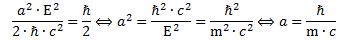
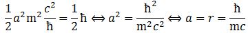
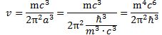
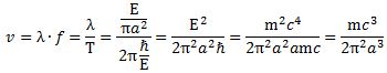
But… Well… What if we use that value as the value for λ? We’d get that linear velocity, right? Let’s try it. The period is equal to T = T = 2π·(ħ/E) = h/E and λ = E/(π·a²), so we write: formula for v We can write this as a function of m and the c and ħ constants only: velocitiy 2

A weird formula but not necessarily nonsensical: we get a finite speed. Now, if the wavelength becomes somewhat less astronomical, we’ll get different values of course. I have a strange feeling that, with these formula, we should, somehow, be able to explain relativistic length contraction. But I will let you think about that as for now. Here I just wanted to show the geometry of the wavefunction a bit more in detail.

[1] The discussions on the mass of neutrinos are interesting in this regard. Scientists all felt the neutrino had to have some (rest) mass, so my instinct on this is theirs. In fact, only recently experimental confirmation came in, and the mass of the known neutrino flavors was estimated to be something like 0.12 eV/c². This mass combines the three known neutrino flavors. To understand this number, you should note it is the same order of magnitude of the equivalent mass of low-energy photons, like infrared or microwave radiation.