Pre-script (dated 26 June 2020): Our ideas have evolved into a full-blown realistic (or classical) interpretation of all things quantum-mechanical. In addition, I note the dark force has amused himself by removing some material. So no use to read this. Read my recent papers instead. 🙂
Original post:
This title sounds very exciting. It is – or was, I should say – one of these things I thought I would never ever understand, until I started studying physics, that is. 🙂
Having said that, there is – incidentally – nothing very special about the Aharonov-Bohm effect. As Feynman puts it: “The theory was known from the beginning of quantum mechanics in 1926. […] The implication was there all the time, but no one paid attention to it.”
To be fair, he also admits the experiment itself – proving the effect – is “very, very difficult”, which is why the first experiment that claimed to confirm the predicted effect was set up in 1960 only. In fact, some claim the results of that experiment were ambiguous, and that it was only in 1986, with the experiment of Akira Tonomura, that the Aharonov-Bohm effect was unambiguously demonstrated. So what is it about?
In essence, it proves the reality of the vector potential—and of the (related) magnetic field. What do we mean with a real field? To put it simply, a real field cannot act on some particle from a distance through some kind of spooky ‘action-at-a-distance’: real fields must be specified at the position of the particle itself and describe what happens there. Now you’ll immediately wonder: so what’s a non-real field? Well… Some field that does act through some kind of spooky ‘action-at-a-distance.’ As for an example… Well… I can’t give you one because we’ve only been discussing real fields so far. 🙂
So it’s about what a magnetic (or an electric) field does in terms influencing motion and/or quantum-mechanical amplitudes. In fact, we discussed this matter quite a while ago (check my 2015 post on it). Now, I don’t want to re-write that post, but let me just remind you of the essentials. The two equations for the magnetic field (B) in Maxwell’s set of four equations (the two others specify the electric field E) are: (1) ∇•B = 0 and (2) c2∇×B = j/ε0 + ∂E/ ∂t. Now, you can temporarily forget about the second equation, but you should note that the ∇•B = 0 equation is always true (unlike the ∇×E = 0 expression, which is true for electrostatics only, when there are no moving charges). So it says that the divergence of B is zero, always.
Now, from our posts on vector calculus, you may or may not remember that the divergence of the curl of a vector field is always zero. We wrote: div (curl A) = ∇•(∇×A) = 0, always. Now, there is another theorem that we can now apply, which says the following: if the divergence of a vector field, say D, is zero – so if ∇•D = 0, then D will be the curl of some other vector field C, so we can write: D = ∇×C. When we now apply this to our ∇•B = 0 equation, we can confidently state the following:
If ∇•B = 0, then there is an A such that B = ∇×A
We can also write this as follows: ∇·B = ∇·(∇×A) = 0 and, hence, B = ∇×A. Now, it’s this vector field A that is referred to as the (magnetic) vector potential, and so that’s what we want to talk about here. As a start, it may be good to write out all of the components of our B = ∇×A vector:
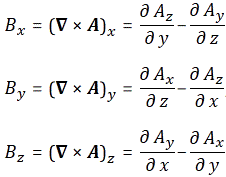
In that 2015 post, I answered the question as to why we’d need this new vector field in a way that wasn’t very truthful: I just said that, in many situations, it would be more convenient – from a mathematical point of view, that is – to first find A, and then calculate the derivatives above to get B.
Now, Feynman says the following about this argument in his Lecture on the topic: “It is true that in many complex problems it is easier to work with A, but it would be hard to argue that this ease of technique would justify making you learn about one more vector field. […] We have introduced A because it does have an important physical significance: it is a real physical field.” Let us follow his argument here.
Quantum-mechanical interference effects
Let us first remind ourselves of the quintessential electron interference experiment illustrated below. [For a much more modern rendering of this experiment, check out the Tout Est Quantique video on it. It’s much more amusing than my rather dry exposé here, but it doesn’t give you the math.]

We have electrons, all of (nearly) the same energy, which leave the source – one by one – and travel towards a wall with two narrow slits. Beyond the wall is a backstop with a movable detector which measures the rate, which we call I, at which electrons arrive at a small region of the backstop at the distance x from the axis of symmetry. The rate (or intensity) I is proportional to the probability that an individual electron that leaves the source will reach that region of the backstop. This probability has the complicated-looking distribution shown in the illustration, which we understand is due to the interference of two amplitudes, one from each slit. So we associate the two trajectories with two amplitudes, which Feynman writes as A1eiΦ1 and A2eiΦ2 respectively.
As usual, Feynman abstracts away from the time variable here because it is, effectively, not relevant: the interference pattern depends on distances and angles only. Having said that, for a good understanding, we should – perhaps – write our two wavefunctions as A1ei(ωt + Φ1) and A2ei(ωt + Φ2) respectively. The point is: we’ve got two wavefunctions – one for each trajectory – even if it’s only one electron going through the slit: that’s the mystery of quantum mechanics. 🙂 We need to add these waves so as to get the interference effect:
R = A1ei(ωt + Φ1) + A2ei(ωt + Φ2) = [A1eiΦ1 + A2eiΦ2]·eiωt
Now, we know we need to take the absolute square of this thing to get the intensity – or probability (before normalization). The absolute square of a product, is the product of the absolute squares of the factors, and we also know that the absolute square of any complex number is just the product of the same number with its complex conjugate. Hence, the absolute square of the eiωt factor is equal to |eiωt|2 = eiωt∙e–iωt = e0 = 1. So the time-dependent factor doesn’t matter: that’s why we can always abstract away from it. Let us now take the absolute square of the [A1eiΦ1 + A2eiΦ2] factor, which we can write as:
|R|2 = |A1eiΦ1 + A2eiΦ2|2 = (A1eiΦ1 + A2eiΦ2)·(A1e–iΦ1 + A2e–iΦ2)
= A12 + A22 + 2·A1·A2·cos(Φ1−Φ2) = A12 + A22 + 2·A1·A2·cosδ with δ = Φ1−Φ2
OK. This is probably going a bit quick, but you should be able to figure it out, especially when remembering that eiΦ + e–iΦ = 2·cosΦ and cosΦ = cos(−Φ). The point to note is that the intensity is equal to the sum of the intensities of both waves plus a correction factor, which is equal to 2·A1·A2·cos(Φ1−Φ2) and, hence, ranges from −2·A1·A2 to +2·A1·A2. Now, it takes a bit of geometrical wizardry to be able to write the phase difference δ = Φ1−Φ2 as
δ = 2π·a/λ = 2π·(x/L)·d/λ
—but it can be done. 🙂 Well… […] OK. 🙂 Let me quickly help you here by copying another diagram from Feynman – one he uses to derive the formula for the phase difference on arrival between the signals from two oscillators. A1 and A2 are equal here (A1 = A2 = A) so that makes the situation below somewhat simpler to analyze. However, instead, we have the added complication of a phase difference (α) at the origin – which Feynman refers to as an intrinsic relative phase.
When we apply the geometry shown above to our electron passing through the slits, we should, of course, equate α to zero. For the rest, the picture is pretty similar as the two-slit picture. The distance a in the two-slit – i.e. the difference in the path lengths for the two trajectories of our electron(s) – is, obviously, equal to the d·sinθ factor in the oscillator picture. Also, because L is huge as compared to x, we may assume that trajectory 1 and 2 are more or less parallel and, importantly, that the triangles in the picture – small and large – are rectangular. Now, trigonometry tells us that sinθ is equal to the ratio of the opposite side of the triangle and the hypotenuse (i.e. the longest side of the rectangular triangle). The opposite side of the triangle is x and, because x is very, very small as compared to L, we may approximate the length of the hypotenuse with L. [I know—a lot of approximations here, but… Well… Just go along with it as for now…] Hence, we can equate sinθ to x/L and, therefore, a = d·x/L. Now we need to calculate the phase difference. How many wavelengths do we have in a? That’s simple: a/λ, i.e. the total distance divided by the wavelength. Now these wavelengths correspond to 2π·a/λ radians (one cycle corresponds to one wavelength which, in turn, corresponds to 2π radians). So we’re done. We’ve got the formula: δ = Φ1−Φ2 = 2π·a/λ = 2π·(x/L)·d/λ.
Huh? Yes. Just think about it. I need to move on. The point is: when x is equal to zero, the two waves are in phase, and the probability will have a maximum. When δ = π, then the waves are out of phase and interfere destructively (cosπ = −1), so the intensity (and, hence, the probability) reaches a minimum.
So that’s pretty obvious – or should be pretty obvious if you’ve understood some of the basics we presented in this blog. We now move to the non-standard stuff, i.e. the Aharonov-Bohm effect(s).
Interference in the presence of an electromagnetic field
In essence, the Aharonov-Bohm effect is nothing special: it is just a law – two laws, to be precise – that tells us how the phase of our wavefunction changes because of the presence of a magnetic and/or electric field. As such, it is not very different from previous analyses and presentations, such as those showing how amplitudes are affected by a potential − such as an electric potential, or a gravitational field, or a magnetic field − and how they relate to a classical analysis of the situation (see, for example, my November 2015 post on this topic). If anything, it’s just a more systematic approach to the topic and – importantly – an approach centered around the use of the vector potential A (and the electric potential Φ). Let me give you the formulas:
The first formula tells us that the phase of the amplitude for our electron (or whatever charged particle) to arrive at some location via some trajectory is changed by an amount that is equal to the integral of the vector potential along the trajectory times the charge of the particle over Planck’s constant. I know that’s quite a mouthful but just read it a couple of times.
The second formula tells us that, if there’s an electrostatic field, it will produce a phase change given by the negative of the time integral of the (scalar) potential Φ.
These two expressions – taken together – tell us what happens for any electromagnetic field, static or dynamic. In fact, they are really the (two) law(s) replacing the F = q(E + v×B) expression in classical mechanics.
So how does it work? Let me further follow Feynman’s treatment of the matter—which analyzes what happens when we’d have some magnetic field in the two-slit experiment (so we assume there’s no electric field: we only look at some magnetic field). We said Φ1 was the phase of the wave along trajectory 1, and Φ2 was the phase of the wave along trajectory 2. Without magnetic field, that is, so B = 0. Now, the (first) formula above tells us that, when the field is switched on, the new phases will be the following:
Hence, the phase difference δ = Φ1−Φ2 will now be equal to:
Now, we can combine the two integrals into one that goes forward along trajectory 1 and comes back along trajectory 2. We’ll denote this path as 1-2 and write the new integral as follows:
Note that we’re using a notation here which suggests that the 1-2 path is closed, which is… Well… Yet another approximation of the Master. In fact, his assumption that the new 1-2 path is closed proves to be essential in the argument that follows the one we presented above, in which he shows that the inherent arbitrariness in our choice of a vector potential function doesn’t matter, but… Well… I don’t want to get too technical here.
Let me conclude this post by noting we can re-write our grand formula above in terms of the flux of the magnetic field B:
So… Well… That’s it, really. I’ll refer you to Feynman’s Lecture on this matter for a detailed description of the 1960 experiment itself, which involves a magnetized iron whisker that acts like a tiny solenoid—small enough to match the tiny scale of the interference experiment itself. I must warn you though: there is a rather long discussion in that Lecture on the ‘reality’ of the magnetic and the vector potential field which – unlike Feynman’s usual approach to discussions like this – is rather philosophical and partially misinformed, as it assumes there is zero magnetic field outside of a solenoid. That’s true for infinitely long solenoids, but not true for real-life solenoids: if we have some A, then we must also have some B, and vice versa. Hence, if the magnetic field (B) is a real field (in the sense that it cannot act on some particle from a distance through some kind of spooky ‘action-at-a-distance’), then the vector potential A is an equally real field—and vice versa. Feynman admits as much as he concludes his rather lengthy philosophical excursion with the following conclusion (out of which I already quoted one line in my introduction to this post):
“This subject has an interesting history. The theory we have described was known from the beginning of quantum mechanics in 1926. The fact that the vector potential appears in the wave equation of quantum mechanics (called the Schrödinger equation) was obvious from the day it was written. That it cannot be replaced by the magnetic field in any easy way was observed by one man after the other who tried to do so. This is also clear from our example of electrons moving in a region where there is no field and being affected nevertheless. But because in classical mechanics A did not appear to have any direct importance and, furthermore, because it could be changed by adding a gradient, people repeatedly said that the vector potential had no direct physical significance—that only the magnetic and electric fields are “real” even in quantum mechanics. It seems strange in retrospect that no one thought of discussing this experiment until 1956, when Bohm and Aharonov first suggested it and made the whole question crystal clear. The implication was there all the time, but no one paid attention to it. Thus many people were rather shocked when the matter was brought up. That’s why someone thought it would be worthwhile to do the experiment to see if it was really right, even though quantum mechanics, which had been believed for so many years, gave an unequivocal answer. It is interesting that something like this can be around for thirty years but, because of certain prejudices of what is and is not significant, continues to be ignored.”
Well… That’s it, folks! Enough for today! 🙂
Some content on this page was disabled on June 16, 2020 as a result of a DMCA takedown notice from The California Institute of Technology. You can learn more about the DMCA here:
https://wordpress.com/support/copyright-and-the-dmca/
Some content on this page was disabled on June 16, 2020 as a result of a DMCA takedown notice from The California Institute of Technology. You can learn more about the DMCA here:
https://wordpress.com/support/copyright-and-the-dmca/
Some content on this page was disabled on June 16, 2020 as a result of a DMCA takedown notice from The California Institute of Technology. You can learn more about the DMCA here:
https://wordpress.com/support/copyright-and-the-dmca/
Some content on this page was disabled on June 16, 2020 as a result of a DMCA takedown notice from The California Institute of Technology. You can learn more about the DMCA here:
https://wordpress.com/support/copyright-and-the-dmca/
Some content on this page was disabled on June 16, 2020 as a result of a DMCA takedown notice from The California Institute of Technology. You can learn more about the DMCA here:
https://wordpress.com/support/copyright-and-the-dmca/
Some content on this page was disabled on June 16, 2020 as a result of a DMCA takedown notice from The California Institute of Technology. You can learn more about the DMCA here:
https://wordpress.com/support/copyright-and-the-dmca/
Some content on this page was disabled on June 16, 2020 as a result of a DMCA takedown notice from The California Institute of Technology. You can learn more about the DMCA here:
https://wordpress.com/support/copyright-and-the-dmca/
Some content on this page was disabled on June 16, 2020 as a result of a DMCA takedown notice from The California Institute of Technology. You can learn more about the DMCA here:
https://wordpress.com/support/copyright-and-the-dmca/
Some content on this page was disabled on June 16, 2020 as a result of a DMCA takedown notice from The California Institute of Technology. You can learn more about the DMCA here:
https://wordpress.com/support/copyright-and-the-dmca/





