Quantum math: the rules – all of them! :-)

Pre-script (dated 26 June 2020): Our ideas have evolved into a full-blown realistic (or classical) interpretation of all things quantum-mechanical. In addition, I note the dark force has amused himself by removing some material. So no use to read this. Read my recent papers instead. 🙂

Original post:

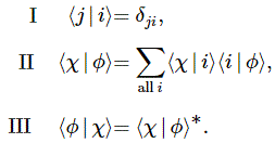
In my previous post, I made no compromise, and used all of the rules one needs to calculate quantum-mechanical stuff:

However, I didn’t explain them. These rules look simple enough, but let’s analyze them now. They’re simple and not at the same time, indeed.

[I] The first equation uses the Kronecker delta, which sounds fancy but it’s just a simple shorthand: δ_ij= δ_jiis equal to 1 if i = j, and zero if i ≠ j, with i and j representing base states. Equation (I) basically says that base states are all different. For example, the angular momentum in the x-direction of a spin-1/2 particle – think of an electron or a proton – is either +ħ/2 or −ħ/2, not something in-between, or some mixture. So 〈 +x | +x 〉 = 〈 −x | −x 〉 = 1 and 〈 +x | −x 〉 = 〈 −x | +x 〉 = 0.

We’re talking base states here, of course. Base states are like a coordinate system: we settle on an x-, y- and z-axis, and a unit, and any point is defined in terms of an x-, y– and z-number. It’s the same here, except we’re talking ‘points’ in four-dimensional spacetime. To be precise, we’re talking constructs evolving in spacetime. To be even more precise, we’re talking amplitudes with a temporal as well as a spatial frequency, which we’ll often represent as:

a·e^−i·θ= e^{−i·(ω·t − k ∙x)} = a·e^{−(i/ħ)·(E·t − p∙x)}

The coefficient in front (a) is just a normalization constant, ensuring all probabilities add up to one. It may not be a constant, actually: perhaps it just ensure our amplitude stays within some kind of envelope, as illustrated below.

As for the ω = E/ħ and k = p/ħ identities, these are the de Broglie equations for a matter-wave, which the young Comte jotted down as part of his 1924 PhD thesis. He was inspired by the fact that the E·t − p∙x factor is an invariant four-vector product (E·t − p∙x = p_μx_μ) in relativity theory, and noted the striking similarity with the argument of any wave function in space and time (ω·t − k ∙x) and, hence, couldn’t resist equating both. Louis de Broglie was inspired, of course, by the solution to the blackbody radiation problem, which Max Planck and Einstein had convincingly solved by accepting that the ω = E/ħ equation holds for photons. As he wrote it:

“When I conceived the first basic ideas of wave mechanics in 1923–24, I was guided by the aim to perform a real physical synthesis, valid for all particles, of the coexistence of the wave and of the corpuscular aspects that Einstein had introduced for photons in his theory of light quanta in 1905.” (Louis de Broglie, quoted in Wikipedia)

Looking back, you’d of course want the phase of a wavefunction to be some invariant quantity, and the examples we gave our previous post illustrate how one would expect energy and momentum to impact its temporal and spatial frequency. But I am digressing. Let’s look at the second equation. However, before we move on, note that minus sign in the exponent of our wavefunction: a·e^−i·θ. The phase turns counter-clockwise. That’s just the way it is. I’ll come back to this.

[II] The φ and χ symbols do not necessarily represent base states. In fact, Feynman illustrates this law using a variety of examples including both polarized as well as unpolarized beams, or ‘filtered’ as well as ‘unfiltered’ states, as he calls it in the context of the Stern-Gerlach apparatuses he uses to explain what’s going on. Let me summarize his argument here.

I discussed the Stern-Gerlach experiment in my post on spin and angular momentum, but the Wikipedia article on it is very good too. The principle is illustrated below: a inhomogeneous magnetic field – note the direction of the gradient ∇B = (∂B/∂x, ∂B/∂y, ∂B/∂z) – will split a beam of spin-one particles into three beams. [Matter-particles with spin one are rather rare (Lithium-6 is an example), but three states (rather than two only, as we’d have when analyzing spin-1/2 particles, such as electrons or protons) allow for more play in the analysis. 🙂 In any case, the analysis is easily generalized.]

The splitting of the beam is based, of course, on the quantized angular momentum in the z-direction (i.e. the direction of the gradient): its value is either ħ, 0, or −ħ. We’ll denote these base states as +, 0 or −, and we should note they are defined in regard to an apparatus with a specific orientation. If we call this apparatus S, then we can denote these base states as +S, 0S and −S respectively.

The interesting thing in Feynman’s analysis is the imagined modified Stern-Gerlach apparatus, which – I am using Feynman‘s words here 🙂 – “puts Humpty Dumpty back together.” It looks a bit monstruous, but it’s easy enough to understand. Quoting Feynman once more: “It consists of a sequence of three high-gradient magnets. The first one (on the left) is just the usual Stern-Gerlach magnet and splits the incoming beam of spin-one particles into three separate beams. The second magnet has the same cross section as the first, but is twice as long and the polarity of its magnetic field is opposite the field in magnet $1$ . The second magnet pushes in the opposite direction on the atomic magnets and bends their paths back toward the axis, as shown in the trajectories drawn in the lower part of the figure. The third magnet is just like the first, and brings the three beams back together again, so that leaves the exit hole along the axis.”

Now, we can use this apparatus as a filter by inserting blocking masks, as illustrated below.

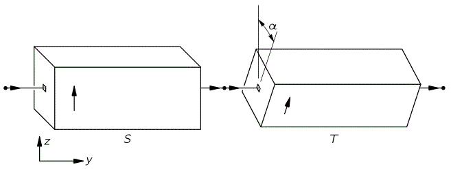
But let’s get back to the lesson. What about the second ‘Law’ of quantum math? Well… You need to be able to imagine all kinds of situations now. The rather simple set-up below is one of them: we’ve got two of these apparatuses in series now, S and T, with T tilted at the angle α with respect to the first.

I know: you’re getting impatient. What about it? Well… We’re finally ready now. Let’s suppose we’ve got three apparatuses in series, with the first and the last one having the very same orientation, and the one in the middle being tilted. We’ll denote them by S, T and S’ respectively. We’ll also use masks: we’ll block the 0 and − state in the S-filter, like in that illustration above. In addition, we’ll block the + and − state in the T apparatus and, finally, the 0 and − state in the S’ apparatus. Now try to imagine what happens: how many particles will get through?

[…]

Just try to think about it. Make some drawing or something. Please!

[…]

OK… The answer is shown below. Despite the filtering in S, the +S particles that come out do have an amplitude to go through the 0T-filter, and so the number of atoms that come out will be some fraction (α) of the number of atoms (N) that came out of the +S-filter. Likewise, some other fraction (β) will make it through the +S’-filter, so we end up with βαN particles.

Now, I am sure that, if you’d tried to guess the answer yourself, you’d have said zero rather than βαN but, thinking about it, it makes sense: it’s not because we’ve got some angular momentum in one direction that we have none in the other. When everything is said and done, we’re talking components of the total angular momentum here, don’t we? Well… Yes and no. Let’s remove the masks from T. What do we get?

[…]

Come on: what’s your guess? N?

[…] You’re right. It’s N. Perfect. It’s what’s shown below.

Now, that should boost your confidence. Let’s try the next scenario. We block the 0 and − state in the S-filter once again, and the + and − state in the T apparatus, so the first two apparatuses are the same as in our first example. But let’s change the S’ apparatus: let’s close the + and − state there now. Now try to imagine what happens: how many particles will get through?

[…]

Come on! You think it’s a trap, isn’t it? It’s not. It’s perfectly similar: we’ve got some other fraction here, which we’ll write as γαN, as shown below.

Next scenario: S has the 0 and − gate closed once more, and T is fully open, so it has no masks. But, this time, we set S’ so it filters the 0-state with respect to it. What do we get? Come on! Think! Please!

[…]

The answer is zero, as shown below.

Does that make sense to you? Yes? Great! Because many think it’s weird: they think the T apparatus must ‘re-orient’ the angular momentum of the particles. It doesn’t: if the filter is wide open, then “no information is lost”, as Feynman puts it. Still… Have a look at it. It looks like we’re opening ‘more channels’ in the last example: the S and S’ filter are the same, indeed, and T is fully open, while it selected for 0-state particles before. But no particles come through now, while with the 0-channel, we had γαN.

Hmm… It actually is kinda weird, won’t you agree? Sorry I had to talk about this, but it will make you appreciate that second ‘Law’ now: we can always insert a ‘wide-open’ filter and, hence, split the beams into a complete set of base states − with respect to the filter, that is − and bring them back together provided our filter does not produce any unequal disturbances on the three beams. In short, the passage through the wide-open filter should not result in a change of the amplitudes. Again, as Feynman puts it: the wide-open filter should really put Humpty-Dumpty back together again. If it does, we can effectively apply our ‘Law’:

For an example, I’ll refer you to my previous post. This brings me to the third and final ‘Law’.

[III] The amplitude to go from state φ to state χ is the complex conjugate of the amplitude to to go from state χ to state φ:

〈 χ | φ 〉 = 〈 φ | χ 〉*

This is probably the weirdest ‘Law’ of all, even if I should say, straight from the start, we can actually derive it from the second ‘Law’, and the fact that all probabilities have to add up to one. Indeed, a probability is the absolute square of an amplitude and, as we know, the absolute square of a complex number is also equal to the product of itself and its complex conjugate:

|z|²= |z|·|z| = z·z*

[You should go through the trouble of reviewing the difference between the square and the absolute square of a complex number. Just write z as a + ib and calculate (a + ib)²= a² + 2abi + b², as opposed to |z|²= a² + b². Also check what it means when writing z as r·e^iθ= r·(cosθ + i·sinθ).]

Let’s applying the probability rule to a two-filter set-up, i.e. the situation with the S and the tilted T filter which we described above, and let’s assume we’ve got a pure beam of +S particles entering the wide-open T filter, so our particles can come out in either of the three base states with respect to T. We can then write:

〈 +T | +S 〉²+ 〈 0T | +S 〉²+ 〈 −T | +S 〉²= 1

⇔ 〈 +T | +S 〉〈 +T | +S 〉* + 〈 0T | +S 〉〈 0T | +S 〉* + 〈 −T | +S 〉〈 −T | +S 〉* = 1

Of course, we’ve got two other such equations if we start with a 0S or a −S state. Now, we take the 〈 χ | φ 〉 = ∑ 〈 χ | i 〉〈 i | φ 〉 ‘Law’, and substitute χ and φ for +S, and all i states for the base states with regard to T. We get:

〈 +S | +S 〉 = 1 = 〈 +S | +T 〉〈 +T | +S 〉 + 〈 +S | 0T 〉〈 0T | +S 〉 + 〈 +S | –T 〉〈 −T | +S 〉

These equations are consistent only if:

〈 +S | +T 〉 = 〈 +T | +S 〉*,

〈 +S | 0T 〉 = 〈 0T | +S 〉*,

〈 +S | −T 〉 = 〈 −T | +S 〉*,

which is what we wanted to prove. One can then generalize to any state φ and χ. However, proving the result is one thing. Understanding it is something else. One can write down a number of strange consequences, which all point to Feynman‘s rather enigmatic comment on this ‘Law’: “If this Law were not true, probability would not be ‘conserved’, and particles would get ‘lost’.” So what does that mean? Well… You may want to think about the following, perhaps. It’s obvious that we can write:

|〈 φ | χ 〉|²= 〈 φ | χ 〉〈 φ | χ 〉* = 〈 χ | φ 〉*〈 χ | φ 〉 = |〈 χ | φ 〉|²

This says that the probability to go from the φ-state to the χ-state is the same as the probability to go from the χ-state to the φ-state.

Now, when we’re talking base states, that’s rather obvious, because the probabilities involved are either 0 or 1. However, if we substitute for +S and −T, or some more complicated states, then it’s a different thing. My guts instinct tells me this third ‘Law’ – which, as mentioned, can be derived from the other ‘Laws’ – reflects the principle of reversibility in spacetime, which you may also interpret as a causality principle, in the sense that, in theory at least (i.e. not thinking about entropy and/or statistical mechanics), we can reverse what’s happening: we can go back in spacetime.

In this regard, we should also remember that the complex conjugate of a complex number in polar form, i.e. a complex number written as r·e^iθ, is equal to r·e^−iθ, so the argument in the exponent gets a minus sign. Think about what this means for our a·e^−i·θ= e^{−i·(ω·t − k ∙x)} = a·e^{−(i/ħ)·(E·t − p∙x)}function. Taking the complex conjugate of this function amounts to reversing the direction of t and x which, once again, evokes that idea of going back in spacetime.

I feel there’s some more fundamental principle here at work, on which I’ll try to reflect a bit more. Perhaps we can also do something with that relationship between the multiplicative inverse of a complex number and its complex conjugate, i.e. z⁻¹= z*/|z|². I’ll check it out. As for now, however, I’ll leave you to do that, and please let me know if you’ve got any inspirational ideas on this. 🙂

So… Well… Goodbye as for now. I’ll probably talk about the Hamiltonian in my next post. I think we really did a good job in laying the groundwork for the really hardcore stuff, so let’s go for that now. 🙂

Post Scriptum: On the Uncertainty Principle and other rules

After writing all of the above, I realized I should add some remarks to make this post somewhat more readable. First thing: not all of the rules are there—obviously! Most notably, I didn’t say anything about the rules for adding or multiplying amplitudes, but that’s because I wrote extensively about that already, and so I assume you’re familiar with that. [If not, see my page on the essentials.]

Second, I didn’t talk about the Uncertainty Principle. That’s because I didn’t have to. In fact, we don’t need it here. In general, all popular accounts of quantum mechanics have an excessive focus on the position and momentum of a particle, while the approach in this and my previous post is quite different. Of course, it’s Feynman’s approach to QM really. Not ‘mine’. 🙂 All of the examples and all of the theory he presents in his introductory chapters in the Third Volume of Lectures, i.e. the volume on QM, are related to things like:

What is the amplitude for a particle to go from spin state +S to spin state −T?
What is the amplitude for a particle to be scattered, by a crystal, or from some collision with another particle, in the θ direction?
What is the amplitude for two identical particles to be scattered in the same direction?
What is the amplitude for an atom to absorb or emit a photon? [See, for example, Feynman’s approach to the blackbody radiation problem.]
What is the amplitude to go from one place to another?

In short, you read Feynman, and it’s only at the very end of his exposé, that he starts talking about the things popular books start with, such as the amplitude of a particle to be at point (x, t) in spacetime, or the Schrödinger equation, which describes the orbital of an electron in an atom. That’s where the Uncertainty Principle comes in and, hence, one can really avoid it for quite a while. In fact, one should avoid it for quite a while, because it’s now become clear to me that simply presenting the Uncertainty Principle doesn’t help all that much to truly understand quantum mechanics.

Truly understanding quantum mechanics involves understanding all of these weird rules above. To some extent, that involves dissociating the idea of the wavefunction with our conventional ideas of time and position. From the questions above, it should be obvious that ‘the’ wavefunction does actually not exist: we’ve got a wavefunction for anything we can and possibly want to measure. That brings us to the question of the base states: what are they?

Feynman addresses this question in a rather verbose section of his Lectures titled: What are the base states of the world? I won’t copy it here, but I strongly recommend you have a look at it. 🙂

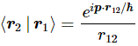
I’ll end here with a final equation that we’ll need frequently: the amplitude for a particle to go from one place (r₁) to another (r₂). It’s referred to as a propagator function, for obvious reasons—one of them being that physicists like fancy terminology!—and it looks like this:

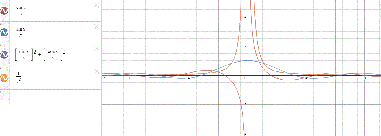
The shape of the e^{(i/ħ)·(p∙r₁₂)}function is now familiar to you. Note the r₁₂in the argument, i.e. the vector pointing from r₁ to r₂. The p∙r₁₂ dot product equals |p|∙|r₁₂|·cosθ = p∙r₁₂·cosθ, with θ the angle between p and r₁₂. If the angle is the same, then cosθ is equal to 1. If the angle is π/2, then it’s 0, and the function reduces to 1/r₁₂. So the angle θ, through the cosθ factor, sort of scales the spatial frequency. Let me try to give you some idea of how this looks like by assuming the angle between p and r₁₂ is the same, so we’re looking at the space in the direction of the momentum only and |p|∙|r₁₂|·cosθ = p∙r₁₂. Now, we can look at the p/ħ factor as a scaling factor, and measure the distance x in units defined by that scale, so we write: x = p∙r₁₂/ħ. The function then reduces to (ħ/p)·e^i∙x/x = (ħ/p)·cos(x)/x + i·(ħ/p)·sin(x)/x, and we just need to square this to get the probability. All of the graphs are drawn hereunder: I’ll let you analyze them. [Note that the graphs do not include the ħ/p factor, which you may look at as yet another scaling factor.] You’ll see – I hope! – that it all makes perfect sense: the probability quickly drops off with distance, both in the positive as well as in the negative x-direction, while it’s going to infinity when very near. [Note that the absolute square, using cos(x)/x and sin(x)/xyields the same graph as squaring 1/x—obviously!]

Some content on this page was disabled on June 16, 2020 as a result of a DMCA takedown notice from The California Institute of Technology. You can learn more about the DMCA here:

https://wordpress.com/support/copyright-and-the-dmca/
Some content on this page was disabled on June 16, 2020 as a result of a DMCA takedown notice from The California Institute of Technology. You can learn more about the DMCA here:

https://wordpress.com/support/copyright-and-the-dmca/
Some content on this page was disabled on June 16, 2020 as a result of a DMCA takedown notice from The California Institute of Technology. You can learn more about the DMCA here:

https://wordpress.com/support/copyright-and-the-dmca/
Some content on this page was disabled on June 16, 2020 as a result of a DMCA takedown notice from The California Institute of Technology. You can learn more about the DMCA here:

https://wordpress.com/support/copyright-and-the-dmca/
Some content on this page was disabled on June 16, 2020 as a result of a DMCA takedown notice from The California Institute of Technology. You can learn more about the DMCA here:

https://wordpress.com/support/copyright-and-the-dmca/
Some content on this page was disabled on June 16, 2020 as a result of a DMCA takedown notice from The California Institute of Technology. You can learn more about the DMCA here:

https://wordpress.com/support/copyright-and-the-dmca/
Some content on this page was disabled on June 16, 2020 as a result of a DMCA takedown notice from The California Institute of Technology. You can learn more about the DMCA here:

https://wordpress.com/support/copyright-and-the-dmca/
Some content on this page was disabled on June 16, 2020 as a result of a DMCA takedown notice from The California Institute of Technology. You can learn more about the DMCA here:

https://wordpress.com/support/copyright-and-the-dmca/

Working with amplitudes

Note (22 May 2020): I am in the process of reviewing many of my posts—including the one below—as a result of my realist interpretation of quantum mechanics, which is based on the ring current model of an electron. It is a delicate exercise because I would like to keep track of the old posts. Perhaps I should copy all of them to some new site. Any case, the point is: I would significantly rephrase some of the below because I now believe spin is very real in quantum mechanics as well.

Original post:

Don’t worry: I am not going to introduce the Hamiltonian matrix—not yet, that is. But this post is going a step further than my previous ones, in the sense that it will be more abstract. At the same time, I do want to stick to real physical examples so as to illustrate what we’re doing when working with those amplitudes. The example that I am going to use involves spin. So let’s talk about that first.

Spin, angular momentum and the magnetic moment

You know spin: it allows experienced pool players to do the most amazing tricks with billiard balls, making a joke of what a so-called elastic collision is actually supposed to look like. So it should not come as a surprise that spin complicates the analysis in quantum mechanics too. We dedicated several posts to that (see, for example, my post on spin and angular momentum in quantum physics) and I won’t repeat these here. Let me just repeat the basics:

1. Classical and quantum-mechanical spin do share similarities: the basic idea driving the quantum-mechanical spin model is that of a electric charge – positive or negative – spinning about its own axis (this is often referred to as intrinsic spin) as well as having some orbital motion (presumably around some other charge, like an electron in orbit with a nucleus at the center). This intrinsic spin, and the orbital motion, give our charge some angular momentum (J) and, because it’s an electric charge in motion, there is a magnetic moment (μ). To put things simply: the classical and quantum-mechanical view of things converge in their analysis of atoms or elementary particles as tiny little magnets. Hence, when placed in an external magnetic field, there is some interaction – a force – and their potential and/or kinetic energy changes. The whole system, in fact, acquires extra energy when placed in an external magnetic field.

Note: The formula for that magnetic energy is quite straightforward, both in classical as well as in quantum physics, so I’ll quickly jot it down: U = −μ•B = −|μ|·|B|·cosθ = −μ·B·cosθ. So it’s just the scalar product of the magnetic moment and the magnetic field vector, with a minus sign in front so as to get the direction right. [θ is the angle between the μ and B vectors and determines whether U as a whole is positive or negative.

2. The classical and quantum-mechanical view also diverge, however. They diverge, first, because of the quantum nature of spin in quantum mechanics. Indeed, while the angular momentum can take on any value in classical mechanics, that’s not the case in quantum mechanics: in whatever direction we measure, we get a discrete set of values only. For example, the angular momentum of a proton or an electron is either −ħ/2 or +ħ/2, in whatever direction we measure it. Therefore, they are referred to as spin-1/2 particles. All elementary fermions, i.e. the particles that constitute matter (as opposed to force-carrying particles, like photons), have spin 1/2.

Note: Spin-1/2 particles include, remarkably enough, neutrons too, which has the same kind of magnetic moment that a rotating negative charge would have. The neutron, in other words, is not exactly ‘neutral’ in the magnetic sense. One can explain this by noting that a neutron is not ‘elementary’, really: it consists of three quarks, just like a proton, and, therefore, it may help you to imagine that the electric charges inside are, somehow, distributed unevenly—although physicists hate such simplifications. I am noting this because the famous Stern-Gerlach experiment, which established the quantum nature of particle spin, used silver atoms, rather than protons or electrons. More in general, we’ll tend to forget about the electric charge of the particles we’re describing, assuming, most of the time, or tacitly, that they’re neutral—which helps us to sort of forget about classical theory when doing quantum-mechanical calculations!

3. The quantum nature of spin is related to another crucial difference between the classical and quantum-mechanical view of the angular momentum and the magnetic moment of a particle. Classically, the angular momentum and the magnetic moment can have any direction.

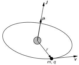
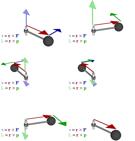
Note: I should probably briefly remind you that J is a so-called axial vector, i.e. a vector product (as opposed to a scalar product) of the radius vector r and the (linear) momentum vector p = m·v, with v the velocity vector, which points in the direction of motion. So we write: J = r×p = r×m·v = |r|·|p|·sinθ·n. The n vector is the unit vector perpendicular to the plane containing r and p (and, hence, v, of course) given by the right-hand rule. I am saying this to remind you that the direction of the magnetic moment and the direction of motion are not the same: the simple illustration below may help to see what I am talking about.]

Back to quantum mechanics: the image above doesn’t work in quantum mechanics. We do not have an unambiguous direction of the angular momentum and, hence, of the magnetic moment. That’s where all of the weirdness of the quantum-mechanical concept of spin comes out, really. I’ll talk about that when discussing Feynman’s ‘filters’ – which I’ll do in a moment – but here I just want to remind you of the mathematical argument that I presented in the above-mentioned post. Just like in classical mechanics, we’ll have a maximum (and, hence, also a minimum) value for J, like +ħ, 0 and +ħ for a Lithium-6 nucleus. [I am just giving this rather special example of a spin-1 article so you’re reminded we can have particles with an integer spin number too!] So, when we measure its angular momentum in any direction really, it will take on one of these three values: +ħ, 0 or +ħ. So it’s either/or—nothing in-between. Now that leads to a funny mathematical situation: one would usually equate the maximum value of a quantity like this to the magnitude of the vector, which is equal to the (positive) square root of J² = J•J = J_x² + J_y² + J_z², with J_x, J_y and J_z the components of J in the x-, y- and z-direction respectively. But we don’t have continuity in quantum mechanics, and so the concept of a component of a vector needs to be carefully interpreted. There’s nothing definite there, like in classical mechanics: all we have is amplitudes, and all we can do is calculate probabilities, or expected values based on those amplitudes.

Huh? Yes. In fact, the concept of the magnitude of a vector itself becomes rather fuzzy: all we can do really is calculate its expected value. Think of it: in the classical world, we have a J² = J•J product that’s independent of the direction of J. For example, if J is all in the x-direction, then J_yand J_zwill be zero, and J² = J_x². If it’s all in the y-direction, then J_xand J_zwill be zero and all of the magnitude of J will be in the y-direction only, so we write: J² = J_y². Likewise, if J does not have any z-component, then our J•J product will only include the x- and y-components: J•J = J_x² + J_y². You get the idea: the J² = J•J product is independent of the direction of J exactly because, in classical mechanics, J actually has a precise and unambiguous magnitude and direction and, therefore, actually has a precise and unambiguous component in each direction. So we’d measure J_x, J_y, and J_zand, regardless of the actual direction of J, we’d find its magnitude |J| = J = +√J² = +(J_x² + J_y² + J_z²)^1/2.

In quantum mechanics, we just don’t have quantities like that. We say that J_x,J_yand J_zhave an amplitude to take on a value that’s equal to +ħ, 0 or +ħ (or whatever other value is allowed by the spin number of the system). Now that we’re talking spin numbers, please note that this characteristic number is usually denoted by j, which is a bit confusing, but so be it. So j can be 0, 1/2, 1, 3/2, etcetera, and the number of ‘permitted values’ is 2j + 1 values, with each value being separated by an amount equal to ħ. So we have 1, 2, 3, 4, 5 etcetera possible values for J_x,J_yand J_zrespectively. But let me get back to the lesson. We just can’t do the same thing in quantum mechanics. For starters, we can’t measure J_x, J_y, and J_zsimultaneously: our Stern-Gerlach apparatus has a certain orientation and, hence, measures one component of J only. So what can we do?

Frankly, we can only do some math here. The wave-mechanical approach does allow to think of the expected value of J² = J•J = J_x² + J_y² + J_z² value, so we write:

E[J²] = E[J•J] = E[J_x² + J_y² + J_z²] = ?

[Feynman’s use of the 〈 and 〉 brackets to denote an expected value is hugely confusing, because these brackets are also used to denote an amplitude. So I’d rather use the more commonly used E[X] notation.] Now, it is a rather remarkable property, but the expected value of the sum of two or more random variables is equal to the sum of the expected values of the variables, even if those variables may not be independent. So we can confidently use the linearity property of the expected value operator and write:

E[J_x²+ J_y² + J_z²] = E[J_x²] + E[J_x²] + E[J_x²]

Now we need something else. It’s also just part of the quantum-mechanical approach to things and so you’ll just have to accept it. It sounds rather obvious but it’s actually quite deep: if we measure the x-, y- or z-component of the angular momentum of a random particle, then each of the possible values is equally likely to occur. So that means, in our case, that the +ħ, 0 or +ħ values are equally likely, so their likelihood is one into three, i.e. 1/3. Again, that sounds obvious but it’s not. Indeed, please note, once again, that we can’t measure J_x, J_y, and J_zsimultaneously, so the ‘or’ in x-, y- or z-component is an exclusive ‘or’. Of course, I must add this equipartition of likelihoods is valid only because we do not have a preferred direction for J: the particles in our beam have random ‘orientations’. Let me give you the lingo for this: we’re looking at an unpolarized beam. You’ll say: so what? Well… Again, think about what we’re doing here: we may of may not assume that the J_x, J_y, and J_zvariables are related. In fact, in classical mechanics, they surely are: they’re determined by the magnitude and direction of J. Hence, they are not random at all ! But let me continue, so you see what comes out.

Because the +ħ, 0 and +ħ values are equally, we can write: E[J_x²] = ħ²/3 + 0/3 + (−ħ)²/3 = [ħ² + 0 + (−ħ)²]/3 = 2ħ²/3. In case you wonder, that’s just the definition of the expected value operator: E[X] = p₁x₁+ p₂x₂+ … = ∑p_ix_i, with p_i the likelihood of the possible value x_i. So we take a weighted average with the respective probabilities as the weights. However, in this case, with an unpolarized beam, the weighted average becomes a simple average.

Now, E[J_y²] and E[J_z²] are – rather unsurprisingly – also equal to 2ħ²/3, so we find that E[J²] = E[J_x²] + E[J_x²] + E[J_x²] = 3·(2ħ²/3) = 2ħ²and, therefore, we’d say that the magnitude of the angular momentum is equal to |J| = J = +√2·ħ ≈ 1.414·ħ. Now that value is not equal to the maximum value of our x-, y-, z-component of J, or the component of J in whatever direction we’d want to measure it. That maximum value is ħ, without the √2 factor, so that’s some 40% less than the magnitude we’ve just calculated!

Now, you’ve probably fallen asleep by now but, what this actually says, is that the angular momentum, in quantum mechanics, is never completely in any direction. We can state this in another way: it implies that, in quantum mechanics, there’s no such thing really as a ‘definite’ direction of the angular momentum.

[…]

OK. Enough on this. Let’s move on to a more ‘real’ example. Before I continue though, let me generalize the results above:

[I] A particle, or a system, will have a characteristic spin number: j. That number is always an integer or a half-integer, and it determines a discrete set of possible values for the component of the angular momentum J in any direction.

[II] The number of values is equal to 2j + 1, and these values are separated by ħ, which is why they are usually measured in units of ħ, i.e. Planck’s reduced constant: ħ ≈ 1×10⁻³⁴J·s, so that’s tiny but real. 🙂 [It’s always good to remind oneself that we’re actually trying to describe reality.] For example, the permitted values for a spin-3/2 particle are +3ħ/2, +ħ/2, −ħ/2 and −3ħ/2 or, measured in units of ħ, +3/2, +1/2, −1/2 and −3/2. When discussing spin-1/2 particles, we’ll often refer to the two possible states as the ‘up’ and the ‘down’ state respectively. For example, we may write the amplitude for an electron or a proton to have a angular momentum in the x-direction equal to +ħ/2 or −ħ/2 as 〈+x〉 and 〈−x〉 respectively. [Don’t worry too much about it right now: you’ll get used to the notation quickly.]

[III] The classical concepts of angular momentum, and the related magnetic moment, have their limits in quantum mechanics. The magnitude of a vector quantity like angular momentum is generally not equal to the maximum value of the component of that quantity in any direction. The general rule is:

J²= j·(j+1)ħ² > j²·ħ²

So the maximum value of any component of J in whatever direction (i.e. j·ħ) is smaller than the magnitude of J (i.e. √[ j·(j+1)]·ħ). This implies we cannot associate any precise and unambiguous direction with quantities like the angular momentum J or the magnetic moment μ. As Feynman puts it:

“That the energy of an atom [or a particle] in a magnetic field can have only certain discrete energies is really not more surprising than the fact that atoms in general have only certain discrete energy levels—something we mentioned often in Volume I. Why should the same thing not hold for atoms in a magnetic field? It does. But it is the attempt to correlate this with the idea of an oriented magnetic moment that brings out some of the strange implications of quantum mechanics.”

**A real example: the disintegration of a muon in a magnetic field**

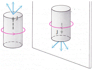
I talked about muon integration before, when writing a much more philosophical piece on symmetries in Nature and time reversal in particular. I used the illustration below. We’ve got an incoming muon that’s being brought to rest in a block of material, and then, as muons do, it disintegrates, emitting an electron and two neutrinos. As you can see, the decay direction is (mostly) in the direction of the axial vector that’s associated with the spin direction, i.e. the direction of the grey dashed line. However, there’s some angular distribution of the decay direction, as illustrated by the blue arrows, that are supposed to visualize the decay products, i.e. the electron and the neutrinos.

This disintegration process is very interesting from a more philosophical side. The axial vector isn’t ‘real’: it’s a mathematical concept—a pseudovector. A pseudo- or axial vector is the product of two so-called true vectors, aka as polar vectors. Just look back at what I wrote about the angular momentum: the J in the J = r×p = r×m·v formula is such vector, and its direction depends on the spin direction, which is clockwise or counter-clockwise, depending from what side you’re looking at it. Having said that, who’s to judge if the product of two ‘true’ vectors is any less ‘true’ than the vectors themselves? 🙂

The point is: the disintegration process does not respect what is referred to as P-symmetry. That’s because our mathematical conventions (like all of these right-hand rules that we’ve introduced) are unambiguous, and they tell us that the pseudovector in the mirror image of what’s going on, has the opposite direction. It has to, as per our definition of a vector product. Hence, our fictitious muon in the mirror should send its decay products in the opposite direction too! So… Well… The mirror image of our muon decay process is actually something that’s not going to happen: it’s physically impossible. So we’ve got a process in Nature here that doesn’t respect ‘mirror’ symmetry. Physicists prefer to call it ‘P-symmetry’, for parity symmetry, because it involves a flip of sign of all space coordinates, so there’s a parity inversion indeed. So there’s processes in Nature that don’t respect it but, while that’s all very interesting, it’s not what I want to write about. [Just check that post of mine if you’d want to read more.] Let me, therefore, use another illustration—one that’s more to the point in terms of what we do want to talk about here:

So we’ve got the same muon here – well… A different one, of course! 🙂 – entering that block (A) and coming to a grinding halt somewhere in the middle, and then it disintegrates in a few micro-seconds, which is an eternity at the atomic or sub-atomic scale. It disintegrates into an electron and two neutrinos, as mentioned above, with some spread in the decay direction. [In case you wonder where we can find muons… Well… I’ll let you look it up yourself.] So we have:

Now it turns out that the presence of a magnetic field (represented by the B arrows in the illustration above) can drastically change the angular distribution of decay directions. That shouldn’t surprise us, of course, but how does it work, exactly? Well… To simplify the analysis, we’ve got a polarized beam here: the spin direction of all muons before they enter the block and/or the magnetic field, i.e. at time t = 0, is in the +x-direction. So we filtered them just, before they entered the block. [I will come back to this ‘filtering’ process.] Now, if the muon’s spin would stay that way, then the decay products – and the electron in particular – would just go straight, because all of the angular momentum is in that direction. However, we’re in the quantum-mechanical world here, and so things don’t stay the same. In fact, as we explained, there’s no such things as a definite angular momentum: there’s just an amplitude to be in the +x state, and that amplitude changes in time and in space.

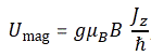
How exactly? Well… We don’t know, but we can apply some clever tricks here. The first thing to note is that our magnetic field will add to the energy of our muon. So, as I explained in my previous post, the magnetic field adds to the E in the exponent of our complex-valued wavefunction a·e^{−(i/ħ)(E·t − p∙x)}. In our example, we’ve got a magnetic field in the z-direction only, so that U = −μ•B reduces to U = −μ_z·B, and we can re-write our wavefunction as:

a·e^{−(i/ħ)[(E+U)·t − p∙x]} = a·e^{−(i/ħ)(E·t − p∙x)}·e^{(i/ħ)(μ_z·B·t)}

Of course, the magnetic field only acts from t = 0 to when the muon disintegrates, which we’ll denote by the point t = τ. So what we get is that the probability amplitude of a particle that’s been in a uniform magnetic field changes by a factor e⁽ⁱ^/ħ)(μ^_z^·B·τ). Note that it’s a factor indeed: we use it to multiply. You should also note that this is a complex exponential, so it’s a periodic function, with its real and imaginary part oscillating between zero and one. Finally, we know that μ_z can take on only certain values: for a spin-1/2 particle, they are plus or minus some number, which we’ll simply denote as μ, so that’s without the subscript, so our factor becomes:

e^{(i/ħ)(±μ·B·t)}

[The plus or minus sign needs to be explained here, so let’s do that quickly: we have two possible states for a spin-1/2 particle, one ‘up’, and the other ‘down’. But then we also know that the phase of our complex-valued wave function turns clockwise, which is why we have a minus sign in the exponent of our e^−iθexpression. In short, for the ‘up’ state, we should take the positive value, i.e. +μ, but the minus sign in the exponent of our e^−iθfunction makes it negative again, so our factor is e^{−(i/ħ)(μ·B·t)}for the ‘up’ state, and e^{+(i/ħ)(μ·B·t)}for the ‘down’ state.]

OK. We get that, but that doesn’t get us anywhere—yet. We need another trick first. One of the most fundamental rules in quantum-mechanics is that we can always calculate the amplitude to go from one state, say φ (read: ‘phi’), to another, say χ (read: ‘khi’), if we have a complete set of so-called base states, which we’ll denote by the index i or j (which you shouldn’t confuse with the imaginary unit, of course), using the following formula:

〈 χ | φ 〉 = ∑ 〈 χ | i 〉〈 i | φ 〉

I know this is a lot to swallow, so let me start with the notation. You should read 〈 χ | φ 〉 from right to left: it’s the amplitude to go from state φ to state χ. This notation is referred to as the bra-ket notation, or the Dirac notation. [Dirac notation sounds more scientific, doesn’t it?] The right part, i.e. | φ 〉, is the bra, and the left part, i.e. 〈 χ | is the ket. In our example, we wonder what the amplitude is for our muon staying in the +x state. Because that amplitude is time-dependent, we can write it as A₊(τ) = 〈 +x at time t = τ | +x at time t = 0 〉 = 〈 +x at t = τ | +x at t = 0 〉or, using a very misleading shorthand, 〈 +x | +x 〉. [The shorthand is misleading because the +x in the ket obviously means something else than the +x in the bra.]

But let’s apply the rule. We’ve got two states with respect to each coordinate axis only here. For example, in respect to the z-axis, the spin values are +z and −z respectively. [As mentioned above, we actually mean that the angular momentum in this direction is either +ħ/2 or −ħ/2, aka as ‘up’ or ‘down’ respectively, but then quantum theorists seem to like all kinds of symbols better, so we’ll use the +z and −z notations for these two base states here. So now we can use our rule and write:

A₊(t) = 〈 +x | +x 〉 = 〈 +x | +z 〉〈 +z | +x 〉 + 〈 +x | −z 〉〈 −z | +x 〉

You’ll say this doesn’t help us any further, but it does, because there is another set of rules, which are referred to as transformation rules, which gives us those 〈 +z | +x 〉 and 〈 −z | +x 〉 amplitudes. They’re real numbers, and it’s the same number for both amplitudes.

〈 +z | +x 〉 = 〈 −z | +x 〉 = 1/√2

This shouldn’t surprise you too much: the square root disappears when squaring, so we get two equal probabilities – 1/2, to be precise – that add up to one which – you guess it – they have to add up to because of the normalization rule: the sum of all probabilities has to add up to one, always. [I can feel your impatience, but just hang in here for a while, as I guide you through what is likely to be your very first quantum-mechanical calculation.] Now, the 〈 +z | +x 〉 = 〈 −z | +x 〉 = 1/√2 amplitudes are the amplitudes at time t = 0, so let’s be somewhat less sloppy with our notation and write 〈 +z | +x 〉 as C₊(0) and 〈 −z | +x 〉 as C₋(0), so we write:

〈 +z | +x 〉 = C₊(0) = 1/√2

〈 −z | +x 〉 = C₋(0) = 1/√2

Now we know what happens with those amplitudes over time: that e^{(i/ħ)(±μ·B·t)} factor kicks in, and so we have:

C₊(t) = C₊(0)·e^{−(i/ħ)(μ·B·t)} = e^{−(i/ħ)(μ·B·t)}/√2

C₋(t) = C₋(0)·e^{+(i/ħ)(μ·B·t)} = e^{+(i/ħ)(μ·B·t)}/√2

As for the plus and minus signs, see my remark on the tricky ± business in regard to μ. To make a long story somewhat shorter :-), our expression for A₊(t) = 〈 +x at t | +x 〉 now becomes:

A₊(t) = 〈 +x | +z 〉·C₊(t) + 〈 +x | −z 〉·C₋(t)

Now, you wouldn’t be too surprised if I’d just tell you that the 〈 +x | +z 〉 and 〈 +x | −z 〉 amplitudes are also real-valued and equal to 1/√2, but you can actually use yet another rule we’ll generalize shortly: the amplitude to go from state φ to state χ is the complex conjugate of the amplitude to to go from state χ to state φ, so we write 〈 χ | φ 〉 = 〈 φ | χ 〉*, and therefore:

〈 +x | +z 〉 = 〈 +z | +x 〉* = (1/√2)* = (1/√2)

〈 +x | −z 〉 = 〈 −z | +x 〉* = (1/√2)* = (1/√2)

So our expression for A₊(t) = 〈 +x at t | +x 〉 now becomes:

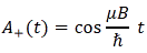
A₊(t) = e^{−(i/ħ)(μ·B·t)}/2 + e^{(i/ħ)(μ·B·t)}/2

That’s the sum of a complex-valued function and its complex conjugate, and we’ve shown more than once (see my page on the essentials, for example) that such sum reduces to the sum of the real parts of the complex exponentials. [You should not expect any explanation of Euler’s e^iθ = cosθ + i·sinθ rule at this level of understanding.] In short, we get the following grand result:

The big question, of course: what does this actually mean? 🙂 Well… Just square this thing and you get the probabilities shown below. [Note that the period of a squared cosine function is π, instead of 2π, which you can easily verify using an online graphing tool.]

Because you’re tired of this business, you probably don’t realize what we’ve just done. It’s spectacular and mundane at the same time. Let me quote Feynman to summarize the results:

“We find that the chance of catching the decay electron in the electron counter varies periodically with the length of time the muon has been sitting in the magnetic field. The frequency depends on the magnetic moment $μ$ . The magnetic moment of the muon has, in fact, been measured in just this way.”

As far as I am concerned, the key result is that we’ve learned how to work with those mysterious amplitudes, and the wavefunction, in a practical way, thereby using all of the theoretical rules of the quantum-mechanical approach to real-life physical situations. I think that’s a great leap forward, and we’ll re-visit those rules in a more theoretical and philosophical démarche in the next post. As for the example itself, Feynman takes it much further, but I’ll just copy the Grand Master here:

Huh? Well… I am afraid I have to leave it at this, as I discussed the precession of ‘atomic’ magnets elsewhere (see my post on precession and diamagnetism), which gives you the same formula: ω_p= μ·B/J (just substitute J for ±ħ/2). However, the derivation above approaches it from an entirely different angle, which is interesting. Of course, all fits. 🙂 However, I’ll let you do your own homework now. I hope to see you tomorrow for the mentioned theoretical discussion. Have a nice evening, or weekend – or whatever ! 🙂

Some content on this page was disabled on June 16, 2020 as a result of a DMCA takedown notice from The California Institute of Technology. You can learn more about the DMCA here:

https://wordpress.com/support/copyright-and-the-dmca/
Some content on this page was disabled on June 16, 2020 as a result of a DMCA takedown notice from The California Institute of Technology. You can learn more about the DMCA here:

https://wordpress.com/support/copyright-and-the-dmca/
Some content on this page was disabled on June 16, 2020 as a result of a DMCA takedown notice from The California Institute of Technology. You can learn more about the DMCA here:

https://wordpress.com/support/copyright-and-the-dmca/
Some content on this page was disabled on June 16, 2020 as a result of a DMCA takedown notice from The California Institute of Technology. You can learn more about the DMCA here:

https://wordpress.com/support/copyright-and-the-dmca/

Quantum mechanics and forces: the classical limit

Original post:

This post continues along the same line as the two previous ones: the objective is to get a better ‘feel’ for those weird amplitudes by showing how they are being affected by a potential − such as an electric potential, or a gravitational field, or a magnetic field − and how they relate to a classical analysis of a situation. It’s what Feynman tries to do too. The best example of such ‘familiarization exercises’, by far, is the comparison between a classical analysis of a force field, and the quantum-mechanical one, so let’s quickly go through that.

The classical situation is depicted below. We’ve got a particle moving in the x-direction and entering a region where the potential − again, think of an electrostatic field, for example, as it probably inspires the V (for voltage, I assume) – varies in the y-direction. As you know, the potential (energy) is measured by doing work against the force, and the work done by the force is the W = ∫F•ds integral along the path. Conversely, one can differentiate both sides of that W = ∫F•ds equation to get the force, so we can write: F = dW/ds. That explains the F = −∂V/∂y expression in the illustration below. Again, think of a positively charged particle that’s being attracted from a high or positive voltage (high V) to a lower or negative voltage.

As a result of the force, the particle is being accelerated transversely, i.e. in the y-direction, and so it adds some momentum in the y-direction (p_y) to the initial momentum p, which is all in the x-direction (p = p_x). Of course, the force only acts as the particle is passing through the area, so that’s during a time interval that’s equal to w/v, with w being the ‘width’ of the area. Now, the vertical momentum builds from 0 to p_y, and we can calculate p_y using Newton’s Law: F = m·a = m·(dv/dt) = d(m·v)/dt = dp/dt. It goes as follows:

We can then use a simple trigonometric formula to find the angle of deflection δθ:

Done! Now we need to show we get the same result with our quantum-mechanical approach or, at the very least, show how our quantum-mechanical approach actually works.

Of course, the assumption is that everything is on a very large scale as compared with the wavelength of our probability amplitudes. We then know that the presence of a potential V will just add to the energy E that we are to use in our wavefunction. Hence, in any small region, the amplitude will vary as:

a·e^{−(i/ħ)[(E_int+ p²/(2m) + V)·t − p∙x]}

Now, in the previous post, we explained that the energy conservation principle does not have any impact on the temporal variation of the wavefunction. Hence, E_int+ p²/(2m) + V effectively remains constant, and the effect of a changing V is on p, and works out through the −p∙x term in the exponent of our complex-valued wave function. To be specific, in a region where V is larger, p will be smaller and, therefore, we’ll have a larger wavelength λ = h/p. [Sorry if you can’t follow here: please do check out what I wrote in my two previous posts. It’s not that difficult.]

The illustration below shows how it works. The wavelength is the distance between successive wave nodes, which you should think of as surfaces where the phase of the amplitude is zero, or as wavefronts. So we’ve got a change in the angle of the wave nodes as well. How does that come about? Look at the two paths a and b: there’s a difference in potential between them, which we denote by ΔV, and which can be approximated as ΔV = (∂V/∂y)·D, with D the separation between the two paths.

Now, if E_int+ p²/(2m) + V is a constant, then ΔV must be equal to −Δ[p²/(2m)]. Now what can we do with that? We’re talking a differential really, so we should apply the Δf(x) = [df(x)/dx]·Δx formula, which gives us:

Δ[p²/(2m)] = (p/m)·Δp = −ΔV ⇔ Δp = −(m/p)·ΔV

[Note that the d[f(x)] = [df(x)/dx]·dx formula is an interesting one: you’ll surely have come across something like Δ[1/λ], and wondered what you could do with that. Now you know: Δ[1/λ] = Δλ/λ².]

Now, we’re interested in Δx, so how can we get some equation for that? Here we need to use the wavenumber k, and the derivation is not so easy—unfortunately! The (p/m)·Δp = −ΔV equation tells us that the wave number will be different along the two paths, and we can write the difference as Δk = Δ(p/ħ) = Δp/ħ. Now, we also now that the wavenumber is expressed in radians per unit distance. In addition, we also know that the wavenumber is the derivative of the phase with respect to distance, so we can approximately calculate the amount by which the phase on path b is ‘ahead’ of the phase on path a as the wave leaves the area, as:

Δ(phase) = Δk·w

Now, Δk = Δp/ħ, so Δ(phase) = Δp·w/ħ = −[m/(p·ħ)]·ΔV·w. Now, along path b, we will have some wavenumber k which, as per the definition of k, is equal to the derivative of the phase with respect to distance, so the ratio of the change in phase along path and the incremental distance Δx should equal the wave number k along path b, so we can write:

Δ(phase)/Δx = k ⇔ Δx = k·Δ(phase) = (λ/2π)·Δ(phase) = (ħ/p)·Δ(phase)

Combining that with Δ(phase) = −[m/(p·ħ)]·ΔV·w identity, we get:

Δx = −(ħ/p)·[m/(p·ħ)]·ΔV·w = −[m/p²]·ΔV·w

Phew! Just hang in there. We’re not done yet. I need to refer to the illustration now to show that Δx can also be approximated by D·δθ, so we write: Δx = D·δθ. [Again: it’s just plain triangle geometry, and the small angle approximation.] Combining both formulas for Δx yields:

δθ = −[m/p²]·ΔV·w/D

Now we can replace p/m by v and use our ΔV = (∂V/∂y)·D approximation to replace ΔV/D by (∂V/∂y), so we get:

δθ = −[1/(p·v)]·(∂V/∂y)·w = −[w/(p·v)]·(∂V/∂y)

So we get the very same equation for δθ as the one we got when applying classical mechanics. That’s a great result—also I have to admit that the differential analysis here was very painful and, hence, difficult to reproduce. In any case, what you should be interested in, is the result: as Feynman summarizes it,

“We get the same particle motions we get from Newton’s $F= m\cdota law$ , provided we assume that a potential contributes a phase to the probability amplitude equal to $V\cdott/ħ$ . Hence, in the classical limit, quantum mechanics agrees with Newtonian mechanics.”

However, he also cautions that “the result we have just got is correct only if the potential variations are slow and smooth”, which actually defines what is referred to as the “classical limit”.

Let me, to conclude this post, present another example out of Feynman’s ‘illustrations’ of what a field or a potential does with amplitudes. Trust me: we’ll need it later. As Feynman is really succinct here, I will just copy it. The quote describes what happens in a magnetic field, as opposed to the electrostatic field which I mentioned above. Just read it: it’s easy. [If it’s too small, just click on it, and the text size will be OK.] However, while it’s easy to understand, the consequences, on which I’ll write a separate post, are quite deep.

So… Well… That’s really it for today. 🙂

Some content on this page was disabled on June 16, 2020 as a result of a DMCA takedown notice from The California Institute of Technology. You can learn more about the DMCA here:

https://wordpress.com/support/copyright-and-the-dmca/
Some content on this page was disabled on June 16, 2020 as a result of a DMCA takedown notice from The California Institute of Technology. You can learn more about the DMCA here:

https://wordpress.com/support/copyright-and-the-dmca/
Some content on this page was disabled on June 16, 2020 as a result of a DMCA takedown notice from The California Institute of Technology. You can learn more about the DMCA here:

https://wordpress.com/support/copyright-and-the-dmca/

Amplitudes, wavefunctions and relativity – or the de Broglie equation re-visited

Original post:

My previous posts were rather technical and, hence, I thought I’d re-visit a topic on which I’ve written before – but represent it from another angle: the de Broglie equation. You know it by heart: it associates a wavelength (λ) with the momentum (p) of a particle: λ = h/p. It’s a simple relationship: the wavelength and the momentum are inversely proportional, and the constant of proportionality is Planck’s constant. It’s an equation you’ll find in all of the popular accounts of quantum mechanics. However, I am of the opinion that the equation may actually not help novices to understand what quantum mechanics is all about—at least not in an initial approach.

One barrier to a proper understanding is that the de Broglie relation is always being presented as the twin of the Planck-Einstein relation for photons, which relates the energy (E) of a photon to its frequency (n): E = h∙ν = ħ∙ω [i]. It’s only natural, then, to try to relate the two equations, as momentum and energy are obviously related one to anotyher. But how exactly? What energy concept should we use? Potential energy? Kinetic energy? Should we include the equivalent energy of the rest mass?

One quickly gets into trouble here. For example, one can try the kinetic energy, K.E. = m∙v²/2 and use the definition of momentum (p = m∙v) to write E = p²/(2m), and then relate the frequency ν to the wavelength λ using the general rule that the traveling speed of a wave is equal to the product of its wavelength and its frequency (v = λ∙ν). But if E = p²/(2m) and ν = v/λ, we get:

p²/(2m) = h∙v/λ ⇔ λ = 2∙h/p

So that is almost right, but not quite: that factor 2 should not be there. In fact, it’s easy to see that we’d get de Broglie’s equation if we’d use E = m∙v² rather than E = m∙v²/2. But E = m∙v²? How could we possibly justify the use of that formula? There’s something weird here—something deep, but I will probably die before I figure out exactly what. 🙂

Note: I should make a reference to the argument of the wavefunction here: E·t −p·x. [The argument of the wavefunction has a 1/ħ factor in front, but we assume we measure both E as well as p in units of ħ here.] So that’s an invariant quantity, i.e. it doesn’t change under a relativistic transformation of the reference frame. Now, if we measure time and distance in equivalent units, so c = 1, then we can show that E/p = 1/v. [Remember: if c would not be one, we’d write: E·β = p·c, with β = v/c, i.e. the relative velocity of our particle, as measured as a ratio of the speed of light.] As E·t − p·x, is an invariant quantity, it’s some constant that’s characteristic of the particle. But x and t change as the clock is tick. Well… Yes. But if we believe the particle is somehow real, and its velocity is v, then the ratio of the real position x and the time t should be equal to v = x/t. Hence, for these very special positions x, i.e. the real position of the particle, we can equate E·t −p·x to E·t −p·v·t = E·t −m·v·v·t = (E − m∙v²)·t. So there we have the m∙v² factor. There must be something very deep about it, but, as mentioned above, I will probably die before I figure out exactly what. 🙂

The second problem is the interpretation of λ. Of course, λ is just a length in space, which we can relate to the spatial frequency or wavenumber k = 2π/λ [ii]. And, of course, the frequency and the wavelength are, once again, related through the traveling speed of the wave: v = λ∙ν. But then, when you think about it, it’s actually not that simple: the wavefunction of a particle is much more complicated. For starters, you should think of it as a wave packet, or wavetrain, i.e. a composite wave: a sum of a potentially infinite number of elementary waves. So we do not have a simple periodic phenomenon here: we need to distinguish the so-called group velocity from the phase velocity, and we’re also talking a complex-valued wavefunction, so it’s all quite different from what we’re used to.

But back to the energy concept. We have Einstein’s E = m∙c² = m₀∙γ∙c² equation, of course, from which the relativistically correct momentum-energy relationship can be derived [iii]:

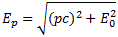
E_pis the energy of a particle with momentum p, and the relationship establishes a one-to-one relationship between the energy and the momentum of a particle [iv], with the rest mass (or rest energy) E₀² = m₀∙c² appearing as a constant (the rest mass does not depend on the reference frame – per definition). However, you can try this formula too, but it will not give you the de Broglie relation. In short, it doesn’t help us in terms of understanding what the de Broglie relation is all about.

So how did this young nobleman, back in 1924, as he was writing his PhD thesis, get this λ = h/p or – using the wavenumber – the k = p/ħ equation?

Well… The relativity theory had been around for quite a while and, amongst other things (including the momentum-energy relationship above), it had also established the invariance of the four-vector product p_μx_μ = E∙t – p∙x = p_μ‘x_μ‘ = E’∙t’ – p’∙x’.

Now, any regular sinusoidal wave is associated with a phase θ = ωt – k∙x, and then quantum theory had associated a complex-valued wavefunction Ψ(θ) = Ψ(ωt – k∙x) with a particle, and so the young count, Louis de Broglie, saw the mathematical similarity between the E∙t – p∙x and ωt – k∙x expressions, and then just took the bold step of substituting ω and k for E/ħ and p/ħ respectively in the Ψ(ωt – k∙x) function. That’s it really: as the laws of physics should look the same, regardless of our frame of reference, he realized the argument of the wavefunction needed to be some invariant quantity, and so that’s what he gets through this substitution.

Of course, the substitution makes sense: it has to. To show why, let’s consider the limiting situation of a particle with zero momentum – so it’s at rest, really – but assuming that the probability of finding it at some point in space, at some point of time is equally distributed over space and time. So we have the rather nonsensical but oft-used wavefunction:

Ψ(θ) = Ψ(x, t) = a·e^iθ = a·e^{i(ωt – k∙x)}

Taking the absolute square of this yields a constant probability equal to a²indeed. The equation is non-sensical or – to put it more politely – a limiting case only because it assumes perfect knowledge about the particle’s momentum p (we said it was zero, exactly) and, hence, about its energy. So we don’t need to worry about any Δ here: Δp = ΔE = 0 and E_p= E₀. As mentioned, we know that doesn’t make much sense, and that a particle in free space will actually be represented by a wave train with a group velocity v (i.e. the classical speed of the particle) and a phase velocity, and so that’s where the modeling of uncertainty comes in, but let’s just go along with the example now. [Note that, while p = 0, that does not imply that E₀ is equal to zero. Indeed, there’s energy in the rest mass and possibly potential energy too!]

Now, if we substitute ω and k for E/ħ and p/ħ respectively – note that we did away with the bold-face k and x, so we’ve reduced the analysis to one dimension (x) only – we get:

Ψ(θ) = Ψ(x, t) = a·e^iθ = a·e^{i(E₀t – p∙x)/ħ}= a·e^i(E₀/ħ)t

What this means is that the phase θ = (E₀/ħ)·t does not depend on x: it only varies in time. Hence, the diagram below – don’t look at the x’ and t’ right now: that’s another reference frame that we’ll introduce in a moment – shows equal-phase lines parallel to the x-axis and, because of the θ = (E₀/ħ)·t equation, they’re equally spaced in time, i.e. in the t-coordinate.

Of course, a particle at rest in one reference frame – let’s say S – will appear to be moving in another – which we’ll denote as S’, so we have the primed coordinates x’ and t’, which are related to the x and t by the Lorentz transformation rules. It’s easy to see that the points of equal phase have a different spacing along the t’-axis, so the frequency in time must be different. Indeed, we’ll write that frequency as ω’ = E_p‘/ħ in the S’ reference frame.

Likewise, we see that the phase now does vary in space, so the probability amplitude does vary in space now, as the particle’s momentum in the primed reference frame is no longer zero: if we write it as p’, then we can write that θ = (E₀/ħ)·t = (E_p‘/ħ)·t − (p/ħ)∙x = (E_p‘/ħ)·t − (p/ħ)∙x. Therefore, our wavefunction becomes:

Ψ(θ) = Ψ(x, t) = a·e^iθ = a·e^i(E₀/ħ)t= Ψ(x’, t’) = a·e^{i(E_p‘·t’ − p’∙x’)/ħ}

We could introduce yet another reference frame, and we’d get similar results. The point is: the k in our Ψ(θ) = Ψ(x, t) = a·e^iθ = a·e^{i(ωt – k∙x)}equation is, effectively, equal to k = p/ħ, and that identity holds in any reference frame.

Now, none of what I wrote above actually proves the de Broglie relation: it merely explains it. When everything is said and done, the de Broglie relation is a hypothesis, but it is an important one—and it does fit into the overall quantum-mechanical or wave-mechanical approach, that physicists take for granted nowadays.

So that’s it, really. I have nothing more to write but I should, perhaps, just remind you about what I said about a ‘particle wave’: we should look at it as some composite wave. Indeed, there will be uncertainty, and the uncertainty in E implies a frequency range Δω = Δ(E/ħ) = ΔE/ħ. Likewise, the momentum will be unknown, and so we’ll have a spread in the wavenumber k as well. We write: Δk = Δ(p/ħ) = Δp/ħ. We can try to reduce this uncertainty, but the Uncertainty Principle gives us the limits: the Δp·Δx and/or the ΔE·Δt products cannot be smaller than ħ/2.

So we’ll have a potentially infinite number of waves with slightly different values for ω and k, whose sum may be visualized as a complex-valued traveling wavetrain, like the lump below.

All of the component waves necessarily need to travel at the same speed, and this speed, which is the ratio of ω and k, will be equal to the so-called phase velocity of the wave (v_p), which we can calculate as v_p= ω/k = (E/ħ)/(p/ħ) = E/p = (m·c²)/(m·v) = c²/v. This speed is superluminal (c²/v = c/β, with β = v/c < 1), but that is not in contradiction with special relativity because the phase velocity carries no ‘signal’ or ‘information’. As for the group velocity (v_g), we can effectively see that this is equal to the classical velocity of our ‘particle’ by noting that:

v_g= dω/dk = d(E/ħ)/d(p/ħ) = dE/dp = d[(p²/(2m)]/dp = p/m = v.

You may think there’s some cheating here, as we equate E with the kinetic energy only. You’re right: the total energy should also include potential energy and rest energy, so E is a sum, but then rest energy and potential energy are treated as constants and, hence, it’s only the kinetic energy that matters when taking the derivative with respect to p, and so that’s why get the result we get, which makes perfect sense.

I wanted this to be a very short post, and so I will effectively end it here. I hope you enjoyed it. It actually sets the stage for a more interesting discussion, and that’s a discussion on how a change in potential energy effectively changes the phase and, hence, the amplitude. But so that’s for next time. I also need to devote a separate post on a discussion of the wave-mechanical framework in general, with a particular focus on the math behind. So… Well… Yes, the next posts are likely to be somewhat more technical again.

[i] I should make a note on notations here, and also insert some definitions. I will denote a frequency by ν (nu), rather than by f, so as to not cause confusion with any function f. A frequency is expressed in cycles per second, while the angular frequency ω is expressed in radians per second. One cycle covers 2π radians and, therefore, we can write: ν = ω/2π. Hence, h∙ν = h∙ω/2π = ħ∙ω. Both ν as well as ω measure the time-rate of change of the phase, as opposed to k, i.e. the spatial frequency of the wave, which depends on the speed of wave. I will also use the symbol v for the speed of a wave, although that is hugely confusing, because I will also use it to denote the classical velocity of the particle. However, I find the conventional use of the symbol of c even more confusing, because this symbol is also used for the speed of light, and the speed of a wave is not necessarily equal to the speed of light. In fact, both the group as well as the phase velocity of a particle wave are very different from the speed of light. The speed of a wave and the speed of light only coincide for electromagnetic waves and, even then, it should be noted that photons also have amplitudes to travel faster or slower than the speed of light.

[ii] Note that the de Broglie relation can be re-written as k = p/ħ, with ħ = h/2π. Indeed, λ = 2π/k and, hence, we get: λ = h/p ⇔ 2π/k = h/p ⇔ p = ħ∙k ⇔ k = p/ħ.

[iii] One gets the equation by equating m to m = m₀γ (γ is the Lorentz factor) in the E² = (mc²)² equation, and re-arranging.

[iv] Note that this energy formula does not include any potential energy: it is (equivalent) rest mass plus kinetic energy only.

Some content on this page was disabled on June 16, 2020 as a result of a DMCA takedown notice from The California Institute of Technology. You can learn more about the DMCA here:

https://wordpress.com/support/copyright-and-the-dmca/

Atomic magnets: precession and diamagnetism

This and the next posts will further build on the concepts introduced in my previous post on particle spin. This post in particular will focus on some of the math we’ll need to understand what quantum mechanics is all about. The first topic is about the quantum-mechanical equivalent of the phenomenon of precession. The other topics are… Well… You’ll see… 🙂

The Larmor frequency

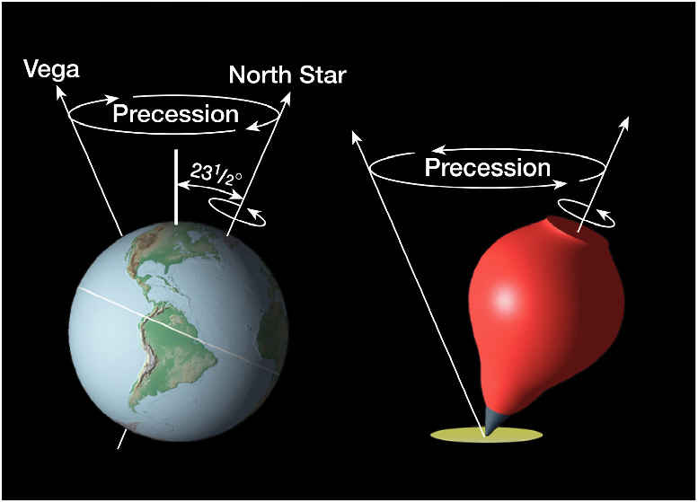
The motion of a spinning object in a force field is quite complicated. In our post on gyroscopes, we introduced the concepts of precession and nutation. The concept of precession is illustrated below for the Earth as well as for a spinning top. In both cases, the external force is just gravity.

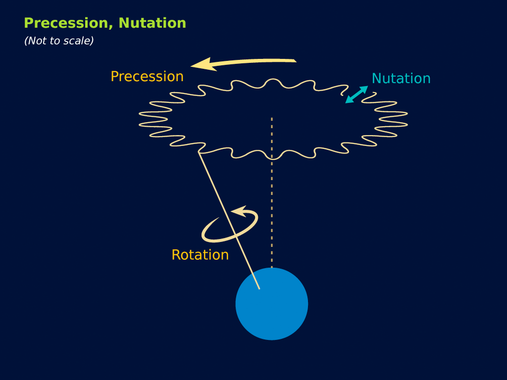
Nutation is an additional movement: on top of the precessional movement, a spinning object may wobble, as illustrated below.

There seems to be no analog for nutation in quantum mechanics. In fact, the terms nutation and precession seem to be used interchangeably in quantum physics, although they are very different in classical physics. But let’s not complicate things and, hence, talk about the phenomenon of precession only.

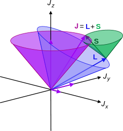
We will not re-explain the phenomenon of precession here but just remind you that the phenomenon can be described in terms of (a) the angle between the symmetry axis and the momentum vector, which we’ll denote by θ, and (b) the angular velocity of the precession, which we’ll denote by ω_p= dφ/dt, as shown below. The J in the illustration below is the angular momentum of the object. Hence, if we’d imagine it to be an electron, then J would be the spin angular momentum only, not its orbital angular momentum—although the analysis would obviously be valid for the orbital and/or total angular momentum as well.

OK. Let’s look at what’s going on. The angular displacement – which is also, rather confusingly, referred to as the angle of precession – in the time interval Δt is, obviously, equal to Δφ = ω_p·Δt. Now, looking at the geometry of the situation, and using the small-angle approximation for the sine, one can also see that ΔJ ≈ (J·sinθ)·(ω_p·Δt). In fact, going to the limit (i.e. for infinitesimally small Δφ and ΔJ), we can write:

dJ/dt = ω_p·J·sinθ

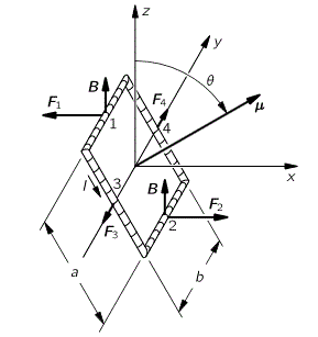
But the angular momentum cannot change if there’s no torque. In fact, the time rate of change of the angular momentum is equal to the torque. [You should look this up but, if you don’t want to do that, note that this is just the equivalent, for rotational motion, of the F = dp/dt law for linear motion.] Now, in my post on magnetic dipoles, I showed that the torque τ on a loop of current with magnetic moment μ in an external magnetic field B is equal to τ = μ×B. So the magnitude of the torque is equal to |τ| = |μ|·|B|·sinθ = μ·B·sinθ. Therefore, ω_p·J·sinθ = μ·B·sinθ and, hence,

ω_p= μ·B/J

However, from the general μ/J = –g·(q_e/2m) equation we derived in our previous post, we know that μ/J – for an atomic magnet, that is – must be equal to μ/J = g·q_e/2m. So we get the formula we wanted to get here:

ω_p= g·(q_e/2m)·B

This equation says that the angular velocity of the precession is proportional to the magnitude of the external magnetic field, and that the constant of proportionality is equal to g·(q_e/2m). It’s good to do the math and actually calculate the precession frequency f_p = ω_p/2π. It’s easy. We had calculated q_e/2m already: it was equal to 1.6×10⁻¹⁹ C divided by 2·9.1×10⁻³¹kg, so that’s 0.0879×10¹² C/kg or 0.0879×10¹²(C·m)/(N·s²), more or less. 🙂 Now, g is dimensionless, and B is expressed in tesla: 1 T = (N·s)/(C·m), so we get the s⁻¹ dimension we want for a frequency. For g = 2 (so we look at the spin of the electron itself only), we get:

f_p = ω_p/2π = 2·0.0879×10¹²/2π ≈ 28×10⁹= 28 gigacycles per tesla = 28 GHz/T

This is a number expressed per unit of the magnetic field strength B. Note that you’ll often see this number expressed as 1.4 megacycles per gauss, using the older gauss unit for magnetic field strength: 1 tesla = 10,000 gauss. For a nucleus, we get a somewhat less impressive number because the proton (or neutron) mass is so much bigger: it’s a number expressed in megacycles per tesla, indeed, and for a proton (i.e. a hydrogen nucleus), it’s about 42.58 MHz/T.

Now, you may wonder about the numbers here. Are they astronomical? Maybe. Maybe not. It’s probably good to note that the strength of the magnetic field in medical MRI systems (magnetic resonance imaging systems) is only 1.5 to 3 tesla, so it’s a rather large unit. You should also note that the clock speed of the CPU in your laptop – so that’s the speed at which it executes instructions – is measured in GHz too, so perhaps it’s not so astronomic. I’ll let you judge. 🙂

So… Well… That’s all nice. The key question, of course, is whether or not this classical view of the electron spinning around a proton is accurate, quantum-mechanically, that is. I’ll let Feynman answer that question provisionally:

“According to the classical theory, then, the electron orbits—and spins—in an atom should precess in a magnetic field. Is it also true quantum-mechanically? It is essentially true, but the meaning of the “precession” is different. In quantum mechanics one cannot talk about the direction of the angular momentum in the same sense as one does classically; nevertheless, there is a very close analogy—so close that we continue to call it precession.”

To distinguish classical and quantum-mechanical precession, quantum-mechanical precession is usually referred to as Larmor precession, and the frequencies above are often referred to as Larmor frequencies. However, I should note that, technically speaking, the term Larmor frequency is actually reserved for the frequency I’ll describe in the next section. I should also note that the ω_p= g·(q_e/2m)·B is usually written, quite simply, as ω_p= γ·B. Of course, the gamma is not the Lorentz factor here, but the so-called gyromagnetic ratio (aka as the magnetogyric ratio): γ = g·(q_e/2m). Oh—just so you know: Sir Joseph Larmor was a British physicists and, yes, he developed all of the stuff we’re talking about here. 🙂

At this point, you may wonder if and why all of the above is relevant. Well… There’s more than one answer to this question, but I’d recommend you start with reading the Wikipedia article on NMR spectroscopy. 🙂 And then you should also read Feynman’s exposé on the Rabi atomic or molecular beam method for determining the precession frequency. It’s really fascinating stuff, but you are sufficiently armed now to read those things for yourself, and so I’ll just move on. Indeed, there’s something else I need to talk about here, and that’s Larmor’s Theorem.

Larmor’s Theorem

We’ve been talking single electrons only so far. Now, you may fear that things become quite complicated when many electrons are involved and… Well… That’s true, of course. And then you may also think that things become even more complicated when external fields are involved, like that external magnetic field we introduced above, and that led our electrons to precess at extraordinary frequencies. Well… That’s not true. Here we get some help: Larmor proved a theorem that basically says that, if we can work out the motions of the electrons without the external field, the solution for the motions with the external field is the no-field solution with an added rotation about the axis of the field. More specifically, for an external magnetic field, the added rotation will have an angular frequency equal to:

ω_L= (q_e/2m)·B

So that’s the same formula as we found for the angular velocity of the precession if g = 1, so that’s very easy to remember. The ω_L frequency, which is the precession frequency for g = 1, is referred to as the Larmor frequency. The proof of the above is remarkably easy, but… Well… I don’t want to copy Feynman here, so I’ll just refer you to the relevant Lecture on it. 🙂

Diamagnetism

I guess it’s about time we relate all of what we learned so far to properties of matter we can relate to, and so that’s what I’ll do here. We’re not going to talk about ferromagnetism here, i.e. the mechanism through which iron, nickel and cobalt and most of their alloys become permanent magnets. That’s quite peculiar and so we will not discuss it here. Here we’ll talk about the very weak quantum-mechanical magnetic effect – a thousand to a million times less than the effects in ferromagnetic materials – that occurs in all materials when placed in an external magnetic field.

While the effect is there in all materials, it’s stronger for some than for others. In fact, it’s usually so weak it is hard to detect, and so it’s usually demonstrated using elements for which the diamagnetic effect is somewhat stronger, like bismuth or antimony. The effect is demonstrated by suspending a piece of material in a non-uniform field, as illustrated below. The diamagnetic effect will cause a small displacement of the material, away from the high-field region, i.e. away from the pointed pole.

I should immediately add that some materials, like aluminium, will actually be attracted to the pointed pole, but that’s because of yet another effect that not all materials share: paramagnetism. I’ll talk about that in another post, together with ferromagnetism. So… Diamagnetism: what is it?

The illustration below shows our spinning electron (q) once again. It also shows a magnetic field B but, unlike our analysis above, or the analysis in our previous post, we assume the external magnetic field is not just there. We assume it changes, because it’s been turned on or off—hopefully slowly: if not, we’d have eddy-current forces causing potentially strong impulses.

But so we’ve got some change in the magnetic flux , and so we know, because of Faraday or Maxwell – you choose 🙂 – that we’ll have some circulation of E, i.e. the electric field. The magnetic flux is B times the surface area, and the circulation is the average tangential component E times the length of the path. Because our model of the orbiting electron is so nice and symmetric, we can write Faraday’s Law here as:

E·2π·r = −d(B·π·r²)/dt ⇔ E = −(r/2)·dB/dt

A field implies a force and, therefore, a torque on the electron. The torque is equal to the force times the lever arm, so it’s equal to (−q_e·E)·r = −q_e·E·r. Of course, the torque is also equal to the rate of the change of the angular momentum, so dJ/dt must equal:

dJ/dt = −q_e·E·r = q_e·(r/2)·(dB/dt)·r = (q_e·r²/2)·(dB/dt)

Now, the assumption is that the field goes from zero to B, so ΔB = B. Therefore, ΔJ must be equal to:

ΔJ = (q_e·r²/2)·B

You should, in fact, derive this more formally, by integrating—but let’s keep things as simple as we can. 🙂 What does this formula say, really? It’s the extra angular momentum from the ‘twist’ that’s given to the electrons as the field is turned on. Now, this added angular momentum makes an extra magnetic moment which, because it is an orbital motion, is just q_e $/2m$ times the angular momentum that’s already there. But more angular momentum means the magnetic moment has changed, according to the μ = (q_e/2m)·J formula we derived in our previous post, so we have:

Δμ = –(q_e/2m)·ΔJ

The minus sign is there because of Lenz’ law: the added momentum is opposite to the magnetic field—and, yes, I know: it’s hard to keep track of all of the conventions involved here. In any case, we get the following grand equation:

So we found that the induced magnetic moment is directly proportional to the magnetic field $B,$ and opposing it. Now that is what explains why our piece of bismuth does what it does in that non-uniform magnetic field. Of course, you’ll say: why is stronger for bismuth than for other materials? And what about aluminium, or paramagnetism in general? Well… Good questions, but we’ll tackle them in the next posts. 🙂

Let me conclude this post by copying Feynman’s little exposé on why the phenomenon of diamagnetism is so particular. In fact, he notes that, because we’re talking a piece of material here that can’t spin – so it’s held in place, so to say – we should have “no magnetic effects whatsoever”. The reasoning is as follows:

This is very interesting indeed. This classical theorem basically says that the energy of a system should not be affected by the presence of a magnetic field. However, we know magnetic effects, such as the diamagnetic effect, are there, so these effects are referred to as ‘quantum-mechanical’ effects indeed: they cannot be explained using classical theory only, even if all of what we wrote above used classical theory only.

I should also note another point: why do we need a non-homogeneous field? Well… The situation is comparable to what we wrote on the Stern-Gerlach experiment. If we would have a homogeneous magnetic field, then we would only have a torque on all of the atomic magnets, but no net force in one or the other direction. There’s something else here too: you may think that the forces pointing towards and away from the pointed tip should cancel each other out, so there should actually be no net movement of the material at all! Feynman’s analysis works for one atom, indeed, but does it still make sense if we look at the whole piece of material? It does, because we’re talking an induced magnetic moment that’s opposing the field, regardless of the orientation of the magnetic moment of the individual atoms in the piece of material. So, even if the individual atoms have opposite momenta, the extra induced magnetic moment will point in the same direction for all. So that solves that issue. However, it does not address Feynman’s own critical remark in regard to the supposed ‘impossibility’ of diamagnetism in classical mechanics.

But I’ll let you think about this, and sign off for today. 🙂 I hope you enjoyed this post.

Some content on this page was disabled on June 16, 2020 as a result of a DMCA takedown notice from The California Institute of Technology. You can learn more about the DMCA here:

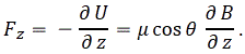
https://wordpress.com/support/copyright-and-the-dmca/
Some content on this page was disabled on June 16, 2020 as a result of a DMCA takedown notice from The California Institute of Technology. You can learn more about the DMCA here:

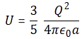
https://wordpress.com/support/copyright-and-the-dmca/
Some content on this page was disabled on June 16, 2020 as a result of a DMCA takedown notice from The California Institute of Technology. You can learn more about the DMCA here:

https://wordpress.com/support/copyright-and-the-dmca/
Some content on this page was disabled on June 16, 2020 as a result of a DMCA takedown notice from The California Institute of Technology. You can learn more about the DMCA here:

https://wordpress.com/support/copyright-and-the-dmca/

Spin and angular momentum in quantum mechanics

Note: A few years after writing the post below, I published a paper on the anomalous magnetic moment which makes (some of) what is written below irrelevant. It gives a clean classical explanation for it. Have a look by clicking on the link here !

Original blog post:

Feynman starts his Volume of Lectures on quantum mechanics (so that’s Volume III of the whole series) with the rules we already know, so that’s the ‘special’ math involving probability amplitudes, rather than probabilities. However, these introductory chapters assume theoretical zero-spin particles, which means they don’t have any angular momentum. While that makes it much easier to understand the basics of quantum math, real elementary particles do have angular momentum, which makes the analysis much more complicated. Therefore, Feynman makes it very clear, after his introductory chapters, that he expects all prospective readers of his third volume to first work their way through chapter 34 and 35 of the second volume, which discusses the angular momentum of elementary particles from both a classical as well as a quantum-mechanical perspective. So that’s what we will do here. I have to warn you, though: while the mentioned two chapters are more generous with text than other textbooks on quantum mechanics I’ve looked at, the matter is still quite hard to digest. By way of introduction, Feynman writes the following:

“The behavior of matter on a small scale—as we have remarked many times—is different from anything that you are used to and is very strange indeed. Understanding of these matters comes very slowly, if at all. One never gets a comfortable feeling that these quantum-mechanical rules are ‘natural’. Of course they are, but they are not natural to our own experience at an ordinary level. The attitude that we are going to take with regard to this rule about angular momentum is quite different from many of the other things we have talked about. We are not going to try to ‘explain’ it but tell you what happens.”

I personally feel it’s not all as mysterious as Feynman claims it to be, but I’ll let you judge for yourself. So let’s just go for it and see what comes out. 🙂

Atomic magnets and the g-factor

When discussing electromagnetic radiation, we introduced the concept of atomic oscillators. It was a very useful model to help us understand what’s supposed to be going on. Now we’re going to introduce atomic magnets. It is based on the classical idea of an electron orbiting around a proton. Of course, we know this classical idea is wrong: we don’t have nice circular electron orbitals, and our discussion on the radius of an the electron in our previous post makes it clear that the idea of the electron itself is rather fuzzy. Nevertheless, the classical concepts used to analyze rotation are also used, mutatis mutandis, in quantum mechanics. Mutatis mutandis means: with necessary alterations. So… Well… Let’s go for it. 🙂 The basic idea is the following: an electron in a circular orbit is a circular current and, hence, it causes a magnetic field, i.e. a magnetic flux through the area of the loop—as illustrated below.

As such, we’ll have a magnetic (dipole) moment, and you may want to review my post(s) on that topic so as to ensure you understand what follows. The magnetic moment (μ) is the product of the current (I) and the area of the loop (π·r²), and its conventional direction is given by the μ vector in the illustration below, which also shows the other relevant scalar and/or vector quantities, such as the velocity v and the orbital angular momentum J. The orbital angular momentum is to be distinguished from the spin angular momentum, which results from the spin around its own axis. So the spin angular momentum – which is often referred to as the spin tout court – is not depicted below, and will only be discussed in a few minutes.

Let me interject something on notation here. Feynman’s always uses J, for whatever momentum. That’s not so usual. Indeed, if you’d google a bit, you’ll see the convention is to use S and L respectively to distinguish spin and orbital angular momentum respectively. If we’d use S and L, we can write the total angular momentum as J = S + L, and the illustration below shows how the S and L vectors are to be added. It looks a bit complicated, so you can skip this for now and come back to it later. But just try to visualize things:

The L vector is moving around, so that assumes the orbital plane is moving around too. That happens when we’d put our atomic system in a magnetic field. We’ll come back to that. In what follows, we’ll assume the orbital plane is not moving.
The S vector here is also moving, which also assumes the axis of rotation is not steady. What’s going on here is referred to as precession, and we discussed it when presenting the math one needs to understand gyroscopes.
Adding S and L yields J, the total angular momentum. Unsurprisingly, this vector wiggles around too. Don’t worry about the magnitudes of the vectors here. Also, in case you’d wonder why the axis of symmetry for the movement of the J vector happens to be the J_z axis, the answer is simple: we chose the coordinate system so as to ensure that was the case.

But I am digressing. I just inserted the illustration above to give you an inkling of where we’re going with this. Indeed, what’s shown above will make it easier for you to see how we can generalize the analysis that we’ll do now, which is an analysis of the orbital angular momentum and the related magnetic moment only. Let me copy the illustration we started with once more, so you don’t have to scroll up to see what we’re talking about.

So we have a charge orbiting around some center. It’s a classical analysis, and so it’s really like a planet around the Sun, except that we should remember that likes repel, and opposites attract, so we’ve got a minus sign in the force law here.

Let’s go through the math. The magnetic moment is the current times the area of the loop. As the velocity is constant, the current is just the charge q times the frequency of rotation. The frequency of rotation is, of course, the velocity (i.e. the distance traveled per second) divided by the circumference of the orbit (i.e. 2π·r). Hence, we write: I = (q_e·v)/(2π·r) and, therefore: μ = (q_e/·v)·π·r²)/(2π·r) = q_e·v·r/2. Note that, as per the convention, current is defined as a flow of positive charges, so the illustration above actually assumes we’re talking some proton in orbit, so q = q_e would be the elementary charge +1. If we’d be talking an electron, then its charge is to be denoted as –q_e(minus q_e, i.e. −1), and we’d need to reverse the direction of μ, which we’ll do in a moment. However, to simplify the discussion, you should just think of some positive charge orbiting the way it does in the illustration above.

OK. That’s all there’s to say about the magnetic moment—for the time being, that is. Let’s think about the angular momentum now. It’s orbital angular momentum here, and so that’s the type of angular momentum we discussed in our post on gyroscopes. We denoted it as L indeed – i.e. not as J, but that’s just a matter of conventions – and we noted that L could be calculated as the vector cross product of the position vector r and the momentum vector p, as shown in the animation below, which also shows the torque vector τ.

The angular momentum L changes in the animation above. In our J case above, it doesn’t. Also, unlike what’s happening with the angular momentum of that swinging ball above, the magnitude of our J doesn’t change. It remains constant, and it’s equal to |J| = J = |r×p| = |r|·|p|·sinθ = r·p = r·m·v. One should note this is a non-relativistic formula, but as the relative velocity of an electron v/c is equal to the fine-structure constant, so that’s α ≈ 0.0073 (see my post on the fine-structure constant if you wonder where this formula comes from), it’s OK to not include the Lorentz factor in our formulas as for now.

Now, as I mentioned already, the illustration we’re using to explain μ and J is somewhat unreal because it assumes a positive charge q, and so μ and J point in the same direction in this case, which is not the case if we’d be talking an actual atomic system with an electron orbiting around a proton. But let’s go along with it as for now and so we’ll put the required minus sign in later. We can combine the J = r·m·v and μ = q·v·r/2 formulas to write:

μ = (q/2m)·J or μ/J = (q/2m) (electron orbit)

In other words, the ratio of the magnetic moment and the angular moment depends on (1) the charge (q) and (2) the mass of the charge, and on those two variables only. So the ratio does not depend on the velocity v nor on the radius r. It can be noted that the q/2m factor is often referred to as the gyromagnetic factor (not to be confused with the g-factor, which we’ll introduce shortly). It’s good to do a quick dimensional check of this relation: the magnetic moment is expressed in ampère per second times the loop area, so that’s (C/s)·m². On the right-hand side, we have the dimension of the gyromagnetic factor, which is C/kg, times the dimension of the angular momentum, which is m·kg·m/s, so we have the same units on both sides: C·m²/s, which is often written as joule per tesla (J/T): the joule is the energy unit (1 J = 1 N·m), and the tesla measures the strength of the magnetic field (1 T = 1 (N·s)/(C·m). OK. So that works out.

So far, so good. The story is a little bit different for the spin angular momentum and the spin magnetic moment. The formula is the following:

μ = (q/m)·J (electron spin)

This formula says that the μ/J ratio is twice what it is for the orbital motion of the electron. Why is that? Feynman says “the reasons are pure quantum-mechanical—there is no classical explanation.” So I’d suggest we just leave that question open for the moment and see if we’re any wiser once we’ve worked ourselves through all of his Lectures on quantum physics. 🙂 Let’s just go along with it as for now.

Now, we can write both formulas – i.e. the formula for the spin and the orbital angular momentum – in a more general way using the format below:

μ = –g·(q_e/2m_e)·J

Why the minus sign? Well… I wanted to get the sign right this time. Our model assumed some positive charge in orbit, but so we want a formula for a atomic system, and so our circling charge should be an electron. So the formula above is the formula for a electron, and the direction of the magnetic moment and of the angular motion will be opposite for electrons: it just replaces q by –q_e. The format above also applies to any atomic system: as Feynman writes, “For an isolated atom, the direction of the magnetic moment will always be exactly opposite to the direction of the angular momentum.” So the $g-factor will be$ characteristic of the state of the atom. It will be $1$ for a pure orbital moment, $2$ for a pure spin moment, or some other number in-between for a complicated system like an atom, indeed.

You may have one last question: why q_e/2m instead of q_e/m in the middle? Well… If we’d take q_e/m, then g would be 1/2 for the orbital angular momentum, and the initial idea with g was that it would be some integer (we’ll quickly see that’s an idea only). So… Well… It’s just one more convention. Of course, conventions are not always respected so sometimes you’ll see the expression above written without the minus sign, so you may see it as μ = g·(q_e/2m_e)·J. In that case, the g-factor for our example involving the spin angular momentum and the spin magnetic moment, will obviously have to be written as minus 2.

Of course, it’s easy to see that the formula for the spin of a proton will look the same, except that we should take the mass of the proton in the formula, so that’s m_pinstead of m_e. Having said that, the elementary charge remains what it is, but so we write it without the minus sign here. To make a long story short, the formula for the proton is:

μ = g·(q_e/2m_p)·J

OK. That’s clear enough. For electrons, the g-factor is referred to as the Landé g-factor, while the g-factor for protons or, more generally, for any spinning nucleus, is referred to as the nuclear g-factor. Now, you may or may not be surprised, but there’s a g-factor for neutrons too, despite the fact that they do not carry a net charge: the explanation for it must have something to do with the quarks that make up the neutron but that’s a complicated matter which we will not get into here. Finally, there is a g-factor for a whole atom, or a whole atomic system, and that’s referred to as… Well… Just the g-factor. 🙂 It’s, obviously, a number that’s characteristic of the state of the atom.

So… This was a big step forward. We’ve got all of the basics on that ‘magical’ spin number here, and so I hope it’s somewhat less ‘magical’ now. 🙂 Let me just copy the values of the g-factor for some elementary particles. It also shows how hard physicists have been trying to narrow down the uncertainty in the measurement. Quite impressive! The table comes from the Wikipedia article on it. I hope the explanations above will now enable you to read and understand that. 🙂

Let’s now move on to the next topic.

Spin numbers and states

Of course, we’re talking quantum mechanics and, therefore, J can only take on a finite number of values. While that’s weird – as weird as other quantum-mechanical things, such as the boson-fermion math, for example – it should not surprise us. As we will see in a moment, the values of J will determine the magnetic energy our system will acquire when we put in some magnetic field and, as Feynman writes: “That the energy of an atom in the magnetic field can have only certain discrete energies is really not more surprising than the fact that atoms in general have only certain discrete energy levels. Why should the same thing not hold for atoms in a magnetic field? It does. It is just correlation of this with the idea of an oriented magnetic moment that brings out some of the strange implications of quantum mechanics.” Yep. That’s true. We’ll talk about that later.

Of course, you’ll probably want some ‘easier’ explanation. I am afraid I can’t give you that. All I can say is that, perhaps, you should think of our discussion on the fine-structure constant, which made it clear that the various radii of the electron, its velocity and its mass and/or energy are all related one to another and, hence, that they can only take on certain values. Indeed, of all the relations we discussed, there’s two you should always remember. The first relationship is the U= (e²/r) = α/r. So that links the energy (which we can express in equivalent mass units), the electron charge and its radius. The second thing you should remember is that the Bohr radius and the classical electron radius are also related through α: α r_e/r = α². So you may want to think of the different values for J as being associated with different ‘orbitals’, so to speak. But that’s a very crude way of thinking about it, so I’d say: just accept the fact and see where it leads us. You’ll see, in a few moments from now, that the whole thing is not unlike the quantum-mechanical explanation of the blackbody radiation problem, which assumes that the permitted energy levels (or states) are equally spaced and h·f apart, with f the frequency of the light that’s being absorbed and/or emitted. So the atom takes up energies only h·f at a time. Here we’ve got something similar: the energy levels that we’ll associate with the discrete values of J – or J‘s components , I should say – will also be equally spaced. Let me show you how it works, as that will make things somewhat more clear.

If we have an object with a given total angular momentum J in classical mechanics, then any of its components x, y or z, could take on any value from +J to −J. That’s not the case here. The rule is that the ‘system’ – the atom, the nucleus, or anything really – will have a characteristic number, which is referred to as the ‘spin’ of the system and, somewhat confusingly, it’s denoted by j (as you can, it’s extremely important, indeed, to distinguish capital letters (like J) from small letters (like j) if you want to keep track of what we’re explaining here). Now, if we have that characteristic spin number j, then any component of J (think of the z-direction, for example) can take on only (one of) the following values:

Note that we will always have 2j + 1 values. For example, if j = 3/2, we’ll have 2·(3/2) + 1 = 4 permitted values, and in the extreme case where j is zero, we’ll still have 2·0 + 1 = 1 permitted value: zero itself. So that basically says we have no angular momentum. […] OK. That should be clear enough, but let’s pause here for a moment and analyze this—just to make sure we ‘get’ this indeed. What’s being written here? What are those numbers? Let’s do a quick dimensional analysis first. Because j, j − 1, j − 2, etcetera are pure numbers, it’s only the dimension of ħ that we need to look at. We know ħ: it’s the Planck constant h, which is expressed in joule·second, i.e. J·s = N·m·s, divided by 2π. That makes sense, because we get the same dimension for the angular momentum. Indeed, the L or J = r·m·v formula also gives us the dimension of physical action, i.e. N·m·s. Just check it: [r]·[m]·[v] = m·kg·m/s = m·(N·s²/m)·m/s = N·m·s. Done!

So we’ve got some kind of unit of action once more here, even if it’s not h but ħ = h/2π. That makes it a quantum of action expressed for a radian, so that’s a unit of length, rather than for a full cycle. Just so you know, ħ = h/2π is 1×10⁻³⁴ J·s ≈ 6.6×10⁻¹⁶ eV·s, and we could chose to express the components of J in terms of h by multiplying the whole thing with 2π. That would boil down to saying that our unit length is not unity but the unit circle, which is 2π times unity. Huh? Just think about it: h is a fundamental unit linked to one full cycle of something, so it all makes sense. Before we move on, you may want to compare the value of h or ħ with the energy of a photon, which is 1.6 to 3.2 eV in the visible light spectrum, but you should note that energy does not have the time dimension, and a second is an eternity in quantum physics, so the comparison is a bit tricky. So… […] Well… Let’s just move on. What about those coefficients? What constraints are there?

Well… The constraint is that the difference between +j and −j must be some integer, so +j−(−j) = 2j must be an integer. That implies that the spin number j is always an integer or a half-integer, depending on whether j is even or odd. Let’s do a few examples:

A lithium (Li-7) nucleus has spin j = 3/2 and, therefore, the permitted values for the angular momentum around any axis (the z-axis, for example) are: 3/2, 3/2−1=1/2, 3/2−2=−1/2, and −3/2—all times ħ of course! Note that the difference between +j and –j is 3, and each ‘step’ between those two levels is ħ, as we’d like it to be.
The nucleus of the much rarer Lithium-6 isotope is one of the few stable nuclei that has spin j = 1, so the permitted values are 1, 0 and −1. Again, all needs to be multiplied with ħ to get the actual value for the J-component that we’re looking at. So each step is ‘one’ again, and the total difference (between +j and –j) is 2.]
An electron is a spin-1/2 particle, and so there are only two permitted values: +ħ/2 and −ħ/2. So there is just one ‘step’ and it’s equal to the whole difference between +j and –j. In fact, this is the most common situation, because we’ll be talking elementary fermions most of the time.
Photons are an example of spin-1 ‘particles’, and ‘particles’ with integer spin are referred to as bosons. In this regard, you may heard of superfluid Helium-4, which is caused by Bose-Einstein condensation near the zero temperature point, and demonstrates the integer spin number of Helium-4, so it resembles Lithium-6 in this regard.

The four ‘typical’ examples makes it clear that the actual situations that we’ll be analyzing will usually be quite simple: we’ll only have 2, 3 or 4 permitted values only. As mentioned, there is this fundamental dichotomy between fermions and bosons. Fermions have half-integer spin, and all elementary fermions, such as protons, neutrons, electrons, neutrinos and quarks are spin-1/2 particles. [Note that a proton and a neutron are, strictly speaking, not elementary, as their constituent parts are quarks.] Bosons have integer spin, and the bosons we know of are spin-one particles, (except for the newly discovered Higgs boson, which is an actual spin-zero particle). The photon is an example, but the helium nucleus (He-4) also has spin one, which – as mentioned above – gives rise to superfluidity when its cooled near the absolute zero point.

In any case, to make a long story short, in practice, we’ll be dealing almost exclusively with spin-1, spin-1/2 particles and, occasionally, with spin-3/2 particles. In addition, to analyze simple stuff, we’ll often pretend particles do not have any spin, so our ‘theoretical’ particles will often be spin zero. That’s just to simplify stuff.

We now need to learn how to do a bit of math with all of this. Before we do so, let me make some additional remarks on these permitted values. Regardless of whether or not J is ‘wobbling’ or moving or not – let me be clear: J is not moving in the analysis above, but we’ll discuss the phenomenon of precession in the next post, and that will involve a J like that J circling around the J_z axis, so I am just preparing the terrain here – J‘s magnitude will always be some constant, which we denoted by |J| = J.

Now there’s something really interesting here, which again distinguishes classical mechanics from quantum mechanics. As mentioned, in classical mechanics, any of J‘s components J_x, J_y or J_z, could take on any value from +J to −J and, therefore, the maximum value of any component of J – say J_z – would be equal to J. To be precise, J would be the value of the component of J in the direction of J itself. So, in classical mechanics, we’d write: |J| = +√(J·J) = +√J² $=$ J, and it would be the maximum value of any component of J. But so we said that, if the spin number of J is j, then the maximum value of any component of J was equal to j·ħ. So, naturally, one would think that J = |J| = +√(J·J) = +√J²= j·ħ.

However, that’s not the case in quantum mechanics: the maximum value of any component of J is not J = j·ħ but the square root of j·(j+1)·ħ.

Huh? Yes. Let me spell it out: |J| = +√(J·J) = +√J²≠ jħ. Indeed, quantum math has many particularities, and this is one of them. The magnitude of J is not equal to the largest possible value of any component of J:

J‘s magnitude is not jħ but √(j(j+1)ħ).

As for the proof of this, let me simplify my life and just copy Feynman here:

The formula can be easily generalized for j ≠ 3/2. Also note that we used a fact that we didn’t mention as yet: all possible values of the z-component (or of whatever component) of J are equally likely.

Now, the result is fascinating, but the implications are even better. Let me paraphrase Feynman as he relates them:

From what we have so far, we can get another interesting and somewhat surprising conclusion. In certain classical calculations the quantity that appears in the final result is the square of the magnitude of the angular momentum $J$ —in other words, $J \cdot J$ = J². It turns out that it is often possible to guess at the correct quantum-mechanical formula by using the classical calculation and the following simple rule: Replace J² $= J \cdot J$ by $j(j+1)ħ$ . This rule is commonly used, and usually gives the correct result.
The second implication is the one we announced already: although we would think classically that the largest possible value of the any component of $J$ is just the magnitude of $J,$ quantum-mechanically the maximum of any component of J is always less than that, because j $ħ is always less than \sqrt(j(j+1)ħ). For example, for j = 3/2 = 1.5, we have j(j+1) = (3/2)\cdot(5/2) = 15/4 = 3.75. Now, the square root of this value is \sqrt3.75 \approx 1.9365, so the magnitude of J is about 30% larger than the maximum value of any of J ‘s components. That’s a pretty spectacular difference, obviously!$

$The second point is quite deep: it implies that the$ angular momentum is ‘never completely along any direction’. Why? Well… Think of it: “any of J‘s components” also includes the component in the direction of J itself! But if the maximum value of that component is 30% less than the magnitude of J, what does that mean really? All we can say is that it implies that the concept of the direction of the magnitude itself is actually quite fuzzy in quantum mechanics! Of course, that’s got to do with the Uncertainty Principle, and so we’ll come back to this later.

In fact, if you look at the math, you may think: what’s that business with those average or expected values? A magnitude is a magnitude, isn’t it? It’s supposed to be calculated from the actual values of J_x, J_y and J_z, not from some average that’s based on the (equal) likelihoods of the permitted values. You’re right. Feynman’s derivation here is quantum-mechanical from the start and, therefore, we get a quantum-mechanical result indeed: the magnitude of J is calculated as the magnitude of a quantum-mechanical variable in the derivation above, not as the magnitude of a classical variable.

[…] OK. On to the next.

The magnetic energy of atoms

Before we start talking about this topic, we should, perhaps, relate the angular momentum to the magnetic moment once again. We can do that using the μ = (q/2m)·J and/or μ = (q/m)·J formula (so that’s the simple formulas for the orbital and spin angular momentum respectively) or, else, by using the more general μ = – g·(q/2m)·J formula.

Let’s use the simpler μ = (q_e/2m)·J formula, which is the one for the orbital angular momentum. What’s q_e/2m? It should be equal to 1.6×10⁻¹⁹ C divided by 2·9.1×10⁻³¹kg, so that’s about 0.0879×10¹² C/kg, or 0.0879×10¹²(C·m)/(N·s²). Now we multiply by ħ/2 ≈ 0.527×10⁻³⁴ J·s. We get something like 0.0463×10⁻²²m²·C/s or J/T. These numbers are ridiculously small, so they’re usually measured in terms of a so-called natural unit: the Bohr magneton, which I’ll explain in a moment but so here we’re interested in its value only, which is μ_B = 9.274×10⁻²⁴J/T. Hence, μ/μ_B = 0.5 = 1/2. What a nice number!

Hmm… This cannot be a coincidence… […] You’re right. It isn’t. To get the full picture, we need to include the spin angular momentum, so we also need to see what the μ = (q/m)·J will yield. That’s easy, of course, as it’s twice the value of (q/2m)·J, so μ/μ_B = 1, and so the total is equal to 3/2. So the magnetic moment of an electron has the same value (when expressed in terms of the Bohr magneton) as the spin (when expressed in terms of ħ). Now that’s just sweet!

Yes, it is. All our definitions and formulas were formulated so as to make it sweet. Having said that, we do have a tiny little problem. If we use the general μ = −g·(q/2m)·J to write the result we found for the spin of the electron only (so we’re not looking at the orbital momentum here), then we’d write: μ = 2·(q/2m)·J = (q/m)·J and, hence, the g-factor here is −2. Yes. We know that. You told me so already. What’s the issue? Well… The problem is: experiments reveal the actual value of g is not exactly −2: it’s −2.00231930436182(52) instead, with the last two digits (in brackets) the uncertainty in the current measurements. Just check it for yourself on the NIST website. 🙂 [Please do check it: it brings some realness to this discussion.]

Hmm…. The accuracy of the measurement suggests we should take it seriously, even if we’re talking a difference of 0.1% only. We should. It can be explained, of course: it’s something quantum-mechanical. However, we’ll talk about this later. As for now, just try to understand the basics here. It’s complicated enough already, and so we’ll stay away from the nitty-gritty as long as we can.

Let’s now get back to the magnetic energy of our atoms. From our discussion on the torque on a magnetic dipole in an external magnetic field, we know that our magnetic atoms will have some extra magnetic energy when placed in an external field. So now we have an external magnetic field B, and we derived the formula for the energy is

U_mag= −μ·B·cosθ = −μ·B

I won’t explain the whole thing once again, but it might help to visualize the situation, which we do below. The loop here is not circular but square, and it’s a current-carrying wire instead of an electron in orbit, but I hope you get the point.

We need to chose some coordinate system to calculate stuff and so we’ll just choose our z-axis along the direction of the external magnetic field B so as to simplify those calculations. If we do that, we can just take the z-component of μ and then combine the interim result with our general μ = – g·(q/2m)·J formula, so we write:

U_mag= −μ_z·B = g·(q/2m)·J_z·B

Now, we know that the maximum value of J_z is equal to j·ħ, and so the maximum value of U_magwill be equal g(q/2m)jħB. Let’s now simplify this expression by choosing some natural unit, and that’s the unit we introduced already above: the Bohr magneton. It’s equal to (q_eħ)/(2m_e) and its value is μ_B ≈ 9.274×10⁻²⁴J/T. So we get the result we wanted, and that is:

Let me make a few remarks here. First on that magneton: you should note there’s also something which is known as the nuclear magneton which, you guessed it, is calculated using the proton charge and the proton mass: μ_N = (q_pħ)/(2m_p) ≈ 5.05×10⁻²⁷J/T. My second remark is a question: what does that formula mean, really? Well… Let me quote Feynman on that. The formula basically says the following:

“The energy of an atomic system is changed when it is put in a magnetic field by an amount that is proportional to the field, and proportional to J_z. We say that the energy of an atomic system is ‘split’ into $2 j + 1$ ‘levels’ by a magnetic field. For instance, an atom whose energy is U₀ outside a magnetic field and whose $j$ is $3/2$ , will have four possible energies when placed in a field. We can show these energies by an energy-level diagram like that drawn below. Any particular atom can have only one of the four possible energies in any given field B. That is what quantum mechanics says about the behavior of an atomic system in a magnetic field.”

Of course, the simplest ‘atomic’ system is a single electron, which has spin 1/2 only (like most fermions really: the example in the diagram above, with spin 3/2, would be that Li-7 system or something similar). If the spin is 1/2, then there are only two energy levels, with J_z = ±ħ/2 and, as we mentioned already, the g-factor for an electron is −2 (again, the use of minus signs (or not) is quite confusing: I am sorry for that), and so our formula above becomes very simple:

U_mag= ± μ_B·B

The graph above becomes the graph below, and we can now speak more loosely and say that the electron either has its spin ‘up’ (so that’s along the field), or ‘down’ (so that’s opposite the field).

By now, you’re probably tired of the math and you’ll wonder: how can we prove all of this permitted value business? Well… That question leads me to the last topic of my post: the Stern-Gerlach experiment.

The Stern-Gerlach experiment

Here again, I can just copy straight of out of Feynman, and so I hope you’ll forgive me if I just do that, as I don’t think there’s any advantage to me trying to summarize what he writes on it:

“The fact that the angular momentum is quantized is such a surprising thing that we will talk a little bit about it historically. It was a shock from the moment it was discovered (although it was expected theoretically). It was first observed in an experiment done in 1922 by Stern and Gerlach. If you wish, you can consider the experiment of Stern-Gerlach as a direct justification for a belief in the quantization of angular momentum. Stern and Gerlach devised an experiment for measuring the magnetic moment of individual silver atoms. They produced a beam of silver atoms by evaporating silver in a hot oven and letting some of them come out through a series of small holes. This beam was directed between the pole tips of a special magnet, as shown in the illustration below. Their idea was the following. If the silver atom has a magnetic moment $μ$ , then in a magnetic field $B$ it has an energy $-μ z B$ , where $z$ is the direction of the magnetic field. In the classical theory, μ_z would be equal to the magnetic moment times the cosine of the angle between the moment and the magnetic field, so the extra energy in the field would be

ΔU = −μ·B·cosθ

Of course, as the atoms come out of the oven, their magnetic moments would point in every possible direction, so there would be all values of $θ$ . Now if the magnetic field varies very rapidly with $z$ —if there is a strong field gradient—then the magnetic energy will also vary with position, and there will be a force on the magnetic moments whose direction will depend on whether cosine $θ$ is positive or negative. The atoms will be pulled up or down by a force proportional to the derivative of the magnetic energy; from the principle of virtual work,

Stern and Gerlach made their magnet with a very sharp edge on one of the pole tips in order to produce a very rapid variation of the magnetic field. The beam of silver atoms was directed right along this sharp edge, so that the atoms would feel a vertical force in the inhomogeneous field. A silver atom with its magnetic moment directed horizontally would have no force on it and would go straight past the magnet. An atom whose magnetic moment was exactly vertical would have a force pulling it up toward the sharp edge of the magnet. An atom whose magnetic moment was pointed downward would feel a downward push. Thus, as they left the magnet, the atoms would be spread out according to their vertical components of magnetic moment. In the classical theory all angles are possible, so that when the silver atoms are collected by deposition on a glass plate, one should expect a smear of silver along a vertical line. The height of the line would be proportional to the magnitude of the magnetic moment. The abject failure of classical ideas was completely revealed when Stern and Gerlach saw what actually happened. They found on the glass plate two distinct spots. The silver atoms had formed two beams.

That a beam of atoms whose spins would apparently be randomly oriented gets split up into two separate beams is most miraculous. How does the magnetic moment know that it is only allowed to take on certain components in the direction of the magnetic field? Well, that was really the beginning of the discovery of the quantization of angular momentum, and instead of trying to give you a theoretical explanation, we will just say that you are stuck with the result of this experiment just as the physicists of that day had to accept the result when the experiment was done. It is an experimental fact that the energy of an atom in a magnetic field takes on a series of individual values. For each of these values the energy is proportional to the field strength. So in a region where the field varies, the principle of virtual work tells us that the possible magnetic force on the atoms will have a set of separate values; the force is different for each state, so the beam of atoms is split into a small number of separate beams. From a measurement of the deflection of the beams, one can find the strength of the magnetic moment.”

I should note one point which Feynman hardly addresses in the analysis above: why do we need a non-homogeneous field? Well… Think of it. The individual silver atoms are not like electrons in some electric field. They are tiny little magnets, and magnets do not behave like electrons. Remember we said there’s no such thing as a magnetic charge? So that applies here. If the silver atoms are tiny magnets, with a magnetic dipole moment, then the only thing they will do is turn, so as to minimize their energy U = −μBcosθ.

That energy is minimized when μ and B are at right angles of each other, so as to make the cosθ factor zero, which happens when θ = π/2. Hence, in a homogeneous magnetic field, we will have a torque on the loop of current – think of our electron(s) in orbit here – but no net force pulling it in this or that direction as a whole. So the atoms would just rotate but not move in our classical analysis here.

To make the atoms themselves move towards or away one of the poles (with or without a sharp tip), the magnetic field must be non-homogeneous, so as to ensure that the force that’s pulling on one side of the loop of current is slightly different from the force that’s pulling (in the opposite direction) on the other side of the loop of current. So that’s why the field has to be non-homogeneous (or inhomogeneous as Feynman calls it), and so that’s why one pole needs to have a sharply pointed tip.

As for the force formula, it’s crucial to remember that energy (or work) is force times distance. To be precise, it’s the ∫F∙ds integral. This integral will have a minus sign in front when we’re doing work against the force, so that’s when we’re increasing the potential energy of an object. Conversely, we’ll just take the positive value when we’re converting potential energy into kinetic energy. So that explains the F = −∂U/∂z formula above. In fact, in the analysis above, Feynman assumes the magnetic moment doesn’t turn at all. That’s pretty obvious from the F_z = −∂U/∂z = −μ∙cosθ∙∂B/∂z formula, in which μ is clearly being treated as a constant. So the F_z in this formula is a net force in the z-direction, and it’s crucially dependent on the variation of the magnetic field in the z-direction. If the field would not be varying, ∂B/∂z would be zero and, therefore, we would not have any net force in the z-direction. As mentioned above, we would only have a torque.

Well… This sort of covers all of what we wanted to cover today. 🙂 I hope you enjoyed it.

Some content on this page was disabled on June 16, 2020 as a result of a DMCA takedown notice from The California Institute of Technology. You can learn more about the DMCA here:

https://wordpress.com/support/copyright-and-the-dmca/
Some content on this page was disabled on June 16, 2020 as a result of a DMCA takedown notice from The California Institute of Technology. You can learn more about the DMCA here:

https://wordpress.com/support/copyright-and-the-dmca/
Some content on this page was disabled on June 16, 2020 as a result of a DMCA takedown notice from The California Institute of Technology. You can learn more about the DMCA here:

https://wordpress.com/support/copyright-and-the-dmca/

Taking the magic out of God’s number: some additional reflections

Note: I have published a paper that is very coherent and fully explains this so-called God-given number. There is nothing magical about it. It is just a scaling constant. Check it out: The Meaning of the Fine-Structure Constant. No ambiguity. No hocus-pocus.

Jean Louis Van Belle, 23 December 2018

Original post:

In my previous post, I explained why the fine-structure constant α is not a ‘magical’ number, even if it relates all fundamental properties of the electron: its mass, its energy, its charge, its radius, its photon scattering cross-section (i.e. the Bohr radius, or the size of the atom really) and, finally, the coupling constant for photon-electron interactions. The key to such understanding of α was the model of an electron as a tiny ball of charge. As such, we have two energy formulas for it. One is the energy that’s needed to assemble the charge from infinitely dispersed infinitesimal charges, which we denoted as U_elec. The other formula is the energy of the field of the tiny ball of charge, which we denoted as E_elec.

The formula for E_elec is calculated using the formula for the field momentum of a moving charge and, using the m = E/c²mas-energy equivalence relationship, is equivalent to the electromagnetic mass. We went through the derivation in our previous post, so let me just jot down the result:

The second formula depends on what ball of charge we’re thinking of, because the formulas for a charged sphere and a spherical shell of charge are different: both have the same structure as the relationship above (so the energy is also proportional to the square of the electron charge and inversely proportional to the radius a), but the constant of proportionality is different. For a sphere of charge, we write:

For a spherical shell of charge we write:

shell

To compare the formulas, you need to note that the square of the electron charge e in the formula for the field energy is equal to e²= q_e²/4πε₀= k_e·q_e². So we multiply the square of the actual electron charge by the Coulomb constant k_e= 1/4πε₀. As you can see, the three formulas have exactly the same form then. It’s just the proportionality constant that’s different: it’s 2/3, 3/5 and 1/2 respectively. It’s interesting to quickly reflect on the dimensions here: [k_e] ≈ 9×10⁹N·m²/C², so e² is expressed in N·m². That makes the units come out alright, as we divide by a (so that’s in meter) and so we get the energy in joule (which is newton·meter). In fact, now that we’re here, let’s quickly calculate the value of e²: it’s that k_e·q_e² product, so it’s equal to 2.3×10⁻²⁸N·m². We can quickly check this value because we know that the classical electron radius is equal to:

So we divide 2.3×10⁻²⁸N·m²by m_ec_²≈ 8.2×10⁻¹⁴J, so we get r₀≈ 2.82×10⁻¹⁵m. So we’re spot on! Why did I do this check? Not really to check what I wrote. It’s more to show what’s going on. We’ve got yet another formula relating the energy and the radius of an electron here, so now we have three. In fact we have more because the formula for U_elec depends on the finer details of our model for the electron (sphere versus shell, uniform versus non-uniform distribution):

E_elec= (2/3)·(e²/a): This is the formula for the energy of the field, so we may all it is external energy.
U_elec= (3/5)·(e²/a), or U_elec= (1/2)·(e²/a): This is the energy needed to assemble our electron, so we might, perhaps, call it its internal energy. The first formula assumes our electron is a uniformly charged sphere. The second assumes all charges sit on the surface of the sphere. If we drop the assumption of the charge having to be uniformly distributed, we’ll find yet another formula.
m_ec²= e²/r₀: This is the energy associated with the so-called classical electron radius (r₀) and the electron’s rest mass (m_e).

In our previous posts, we assumed the last equation was the right one. Why? Because it’s the one that’s been verified experimentally. The discrepancies between the various proportionality coefficients – i.e. the difference between 2/3 and 1, basically – are to be explained because of the binding forces within the electron, without which the electron would just ‘explode’, as the French physicist and polymath Henri Poincaré famously put it. Indeed, if the electron is a little ball of negative charge, the repulsive forces between its parts should rip it apart. So we will not say anything more about this. You can have fun yourself by googling all the various theories that try to model these binding forces. [I may do the same some day, but now I’ve got other priorities: I want to move to Feynman’s third volume of Lectures, which is devoted to quantum physics only, so I look very much forward to that.]

In this post, I just wanted to reflect once more on what constants are really fundamental and what constants are somewhat less fundamental. From all what I wrote in my previous post, I said there were three:

The fine-structure constant α, which is a dimensionless number.
Planck’s constant h, whose dimension is joule·second, so that’s the dimension of action.
The speed of light c, whose dimension is that of a velocity.

The three are related through the following expression:

This is an interesting expression. Let’s first check its dimension. We already explained that e_² is expressed in N·m². That’s rather strange, because it means the dimension of e itself is N^1/2·m: what’s the square root of a force of one newton? In fact, to interpret the formula above, it’s probably better to re-write e²as e²= q_e²/4πε₀= k_e·q_e². That shows you how the electron charge and Coulomb’s constant are related. Of course, they are part and parcel of one and the same force law: Coulomb’s law. We don’t need anything else, except for relativity theory, because we need to explain the magnetic force as well—and that we can do because magnetism is just a relativistic effect. Think of the field momentum indeed: the magnetic field comes into play only when we start to move our electron. The relativity effect is captured by c in that formula for α above. As for ħ, ħ = h/2π comes with the E = h·f equation, which links us to the electron’s Compton wavelength λ through the de Broglie relation λ = h/p.

The point is: we should probably not look at α as a ‘fundamental physical constant’. It’s e² that’s the third fundamental constant, besides h and c. Indeed, it’s from e² that all the rest follows: the electron’s internal energy, its external energy, and its radius, and then all the rest by combining stuff with other stuff.

Now, we took the magic out of α by doing what we did in the previous posts, and that’s to combine stuff with other stuff, and so now you may think I am putting the magic back in with that formula for α, which seems to define α in terms of the three mentioned ‘fundamental’ constants. That’s not the case: this relation comes out of all of the other relationships we found, and so it’s nothing new really. It’s actually not a definition of α: it just does what it does, and that’s to relate α to the ‘fundamental’ physical constants behind.

So… No new magic. In fact, I want to close this post by taking away even more of the magic. If you read my previous post, I said that α was ‘God’s cut-off factor’ 🙂 ensuring our energy functions do not blow up, but I also said it was impossible to say why he chose 0.00729735256 as the cut-off factor. The question is actually easily answered by thinking about those two formulas we had for the internal and external energy respectively. Let’s re-write them in natural units and, temporarily, two different subscripts for α, so we write:

E_elec= α_e/r₀: This is the formula for the energy of the field.
U_elec= α_u/r₀: This is the energy needed to assemble our electron.

Both energies are determined by the above-mentioned laws, i.e. Coulomb’s Law and the theory of relativity, so α has got nothing to do what that. However, both energies have to be the same, and so α_ehas to be equal to α_u. In that sense, α is, quite simply, a proportionality constant that achieves that equality. Now that explains why we can derive α from the three other constants which, as mentioned above, are probably more fundamental. In fact, we’ve got only three degrees of freedom here, so if we chose c, h and e as ‘fundamental’, then α isn’t any more.

The underlying deep question behind it all is why those two energies should be equal. Why would our electron have some internal energy if it’s elementary? The answer to that question is: because it has some non-zero radius, and it has some non-zero radius because we don’t want our formula for the field energy (or the field momentum) to blow up. Now, if it has some radius, then it has to have some internal energy.

You’ll say: that makes sense, but it doesn’t answer the question. Why would it have internal energy, with or without a zero radius? If an electron is an elementary particle, then it’s really elementary, isn’t? And so then we shouldn’t try to ‘assemble’ it from an infinite number of infinitesimally small charges. You’re right, and here we can also note that the fact that the electron doesn’t blow up is firm evidence it’s very elementary indeed.

I should also note that Feynman actually doesn’t talk about the energy that’s needed to assemble a charge: he gets his U_elec= (1/2)·(e²/a) by calculating the external field energy for a spherical shell of charge, and he sticks to it—presumably because it’s the same field for a uniform or non-uniform sphere of charge. He only notes there has to be some radius because, if not, the formula he uses blows up, indeed. So – who knows? – perhaps he doesn’t quite believe that formula for the internal energy is relevant either.

So perhaps there is no internal energy indeed. Perhaps there’s just the energy of the field. So… Well… I can’t say much about this… Except… Well… Perhaps just one more thing. Let me note something that, I hope, you noticed as well: the k_e·q_e²is the numerator in Coulomb’s Law itself. You also know that energy equals force times distance. So if we divide both sides by r₀, we get Coulomb’s Law itself F_elec= k_e·q_e²/r₀². The only thing is: what’s the distance? It’s one charge only, and there is no distance between one charge, is there? Well… Yes and no. I have been thinking that the requirement of the internal and external energies being equal resembles the statement that the forces between two charges are equal and opposite. That ties in with the idea of the internal energy itself: remember we were basically talking forces between infinitesimally small elements of charge within the electron itself? So r₀ is, perhaps, some average distance or so. There must be some way of thinking of it like that. But… Well… Which one exactly?

This kind of reflection may not make sense. Who knows? I obviously need to think all of this through and so this post is, indeed, just a bunch of reflections for which I will have more time later—hopefully. 🙂 Perhaps we’re all just pushing the matter too far. Perhaps we should just accept that the external energy has that 2/3 factor but that the actual energy of the electron should also include the equivalent energy of some binding force that holds the electron together. Well… In any case. That’s all I am going to do on this extremely complicated matter. It’s time to move indeed! So the point to take home here is probably just this:

When calculating the radius of an electron using classical theory, we get in trouble: not only do we find different radii, but the radii that we find do not respect the E = m_ec²law. It’s only the m_ec²= e²/r₀ that’s relativistically correct.
That suggests the electron also has some non-electric mass, which are referred to as ‘binding forces’ or ‘Poincaré stresses’, but which remain to be explained convincingly.
All of this shouldn’t surprise us: for all we know, the electron is something fuzzy. 🙂

So my next posts will focus on the ‘essentials’ preparing for Feynman’s Volume on quantum mechanics. Those ‘essentials’ will still involve some classical stuff but, as you will see, even more contradictions, that – hopefully! – will then be solved in the quantum-mechanical picture of it all. 🙂

Some content on this page was disabled on June 16, 2020 as a result of a DMCA takedown notice from The California Institute of Technology. You can learn more about the DMCA here:

https://wordpress.com/support/copyright-and-the-dmca/
Some content on this page was disabled on June 20, 2020 as a result of a DMCA takedown notice from Michael A. Gottlieb, Rudolf Pfeiffer, and The California Institute of Technology. You can learn more about the DMCA here:

https://wordpress.com/support/copyright-and-the-dmca/
Some content on this page was disabled on June 20, 2020 as a result of a DMCA takedown notice from Michael A. Gottlieb, Rudolf Pfeiffer, and The California Institute of Technology. You can learn more about the DMCA here:

https://wordpress.com/support/copyright-and-the-dmca/