I re-visited the Uncertainty Principle a couple of times already, but here I really want to get at the bottom of the thing? What’s uncertain? The energy? The time? The wavefunction itself? These questions are not easily answered, and I need to warn you: you won’t get too much wiser when you’re finished reading this. I just felt like freewheeling a bit. [Note that the first part of this post repeats what you’ll find on the Occam page, or my post on Occam’s Razor. But these post do not analyze uncertainty, which is what I will be trying to do here.]
Let’s first think about the wavefunction itself. It’s tempting to think it actually is the particle, somehow. But it isn’t. So what is it then? Well… Nobody knows. In my previous post, I said I like to think it travels with the particle, but then doesn’t make much sense either. It’s like a fundamental property of the particle. Like the color of an apple. But where is that color? In the apple, in the light it reflects, in the retina of our eye, or is it in our brain? If you know a thing or two about how perception actually works, you’ll tend to agree the quality of color is not in the apple. When everything is said and done, the wavefunction is a mental construct: when learning physics, we start to think of a particle as a wavefunction, but they are two separate things: the particle is reality, the wavefunction is imaginary.
But that’s not what I want to talk about here. It’s about that uncertainty. Where is the uncertainty? You’ll say: you just said it was in our brain. No. I didn’t say that. It’s not that simple. Let’s look at the basic assumptions of quantum physics:
- Quantum physics assumes there’s always some randomness in Nature and, hence, we can measure probabilities only. We’ve got randomness in classical mechanics too, but this is different. This is an assumption about how Nature works: we don’t really know what’s happening. We don’t know the internal wheels and gears, so to speak, or the ‘hidden variables’, as one interpretation of quantum mechanics would say. In fact, the most commonly accepted interpretation of quantum mechanics says there are no ‘hidden variables’.
- However, as Shakespeare has one of his characters say: there is a method in the madness, and the pioneers– I mean Werner Heisenberg, Louis de Broglie, Niels Bohr, Paul Dirac, etcetera – discovered that method: all probabilities can be found by taking the square of the absolute value of a complex-valued wavefunction (often denoted by Ψ), whose argument, or phase (θ), is given by the de Broglie relations ω = E/ħ and k = p/ħ. The generic functional form of that wavefunction is:
Ψ = Ψ(x, t) = a·e−iθ = a·e−i(ω·t − k ∙x) = a·e−i·[(E/ħ)·t − (p/ħ)∙x]
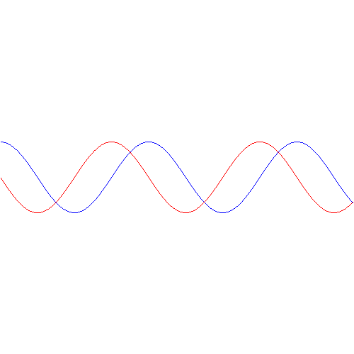
That should be obvious by now, as I’ve written more than a dozens of posts on this. 🙂 I still have trouble interpreting this, however—and I am not ashamed, because the Great Ones I just mentioned have trouble with that too. It’s not that complex exponential. That e−iφ is a very simple periodic function, consisting of two sine waves rather than just one, as illustrated below. [It’s a sine and a cosine, but they’re the same function: there’s just a phase difference of 90 degrees.] 
No. To understand the wavefunction, we need to understand those de Broglie relations, ω = E/ħ and k = p/ħ, and then, as mentioned, we need to understand the Uncertainty Principle. We need to understand where it comes from. Let’s try to go as far as we can by making a few remarks:
- Adding or subtracting two terms in math, (E/ħ)·t − (p/ħ)∙x, implies the two terms should have the same dimension: we can only add apples to apples, and oranges to oranges. We shouldn’t mix them. Now, the (E/ħ)·t and (p/ħ)·x terms are actually dimensionless: they are pure numbers. So that’s even better. Just check it: energy is expressed in newton·meter (energy, or work, is force over distance, remember?) or electronvolts (1 eV = 1.6×10⁻¹⁹ J = 1.6×10⁻¹⁹ N·m); Planck’s constant, as the quantum of action, is expressed in J·s or eV·s; and the unit of (linear) momentum is 1 N·s = 1 kg·m/s = 1 N·s. E/ħ gives a number expressed per second, and p/ħ a number expressed per meter. Therefore, multiplying E/ħ and p/ħ by t and x respectively gives us a dimensionless number indeed.
- It’s also an invariant number, which means we’ll always get the same value for it, regardless of our frame of reference. As mentioned above, that’s because the four-vector product pμxμ = E·t − p∙x is invariant: it doesn’t change when analyzing a phenomenon in one reference frame (e.g. our inertial reference frame) or another (i.e. in a moving frame).
- Now, Planck’s quantum of action h, or ħ – h and ħ only differ in their dimension: h is measured in cycles per second, while ħ is measured in radians per second: both assume we can at least measure one cycle – is the quantum of energy really. Indeed, if “energy is the currency of the Universe”, and it’s real and/or virtual photons who are exchanging it, then it’s good to know the currency unit is h, i.e. the energy that’s associated with one cycle of a photon. [In case you want to see the logic of this, see my post on the physical constants c, h and α.]
- It’s not only time and space that are related, as evidenced by the fact that t − x itself is an invariant four-vector, E and p are related too, of course! They are related through the classical velocity of the particle that we’re looking at: E/p = c2/v and, therefore, we can write: E·β = p·c, with β = v/c, i.e. the relative velocity of our particle, as measured as a ratio of the speed of light. Now, I should add that the t − x four-vector is invariant only if we measure time and space in equivalent units. Otherwise, we have to write c·t − x. If we do that, so our unit of distance becomes c meter, rather than one meter, or our unit of time becomes the time that is needed for light to travel one meter, then c = 1, and the E·β = p·c becomes E·β = p, which we also write as β = p/E: the ratio of the energy and the momentum of our particle is its (relative) velocity.
Combining all of the above, we may want to assume that we are measuring energy and momentum in terms of the Planck constant, i.e. the ‘natural’ unit for both. In addition, we may also want to assume that we’re measuring time and distance in equivalent units. Then the equation for the phase of our wavefunctions reduces to:
θ = (ω·t − k ∙x) = E·t − p·x
Now, θ is the argument of a wavefunction, and we can always re-scale such argument by multiplying or dividing it by some constant. It’s just like writing the argument of a wavefunction as v·t–x or (v·t–x)/v = t –x/v with v the velocity of the waveform that we happen to be looking at. [In case you have trouble following this argument, please check the post I did for my kids on waves and wavefunctions.] Now, the energy conservation principle tells us the energy of a free particle won’t change. [Just to remind you, a ‘free particle’ means it’s in a ‘field-free’ space, so our particle is in a region of uniform potential.] So we can, in this case, treat E as a constant, and divide E·t − p·x by E, so we get a re-scaled phase for our wavefunction, which I’ll write as:
φ = (E·t − p·x)/E = t − (p/E)·x = t − β·x
Alternatively, we could also look at p as some constant, as there is no variation in potential energy that will cause a change in momentum, and the related kinetic energy. We’d then divide by p and we’d get (E·t − p·x)/p = (E/p)·t − x) = t/β − x, which amounts to the same, as we can always re-scale by multiplying it with β, which would again yield the same t − β·x argument.
The point is, if we measure energy and momentum in terms of the Planck unit (I mean: in terms of the Planck constant, i.e. the quantum of energy), and if we measure time and distance in ‘natural’ units too, i.e. we take the speed of light to be unity, then our Platonic wavefunction becomes as simple as:
Φ(φ) = a·e−iφ = a·e−i(t − β·x)
This is a wonderful formula, but let me first answer your most likely question: why would we use a relative velocity?Well… Just think of it: when everything is said and done, the whole theory of relativity and, hence, the whole of physics, is based on one fundamental and experimentally verified fact: the speed of light is absolute. In whatever reference frame, we will always measure it as 299,792,458 m/s. That’s obvious, you’ll say, but it’s actually the weirdest thing ever if you start thinking about it, and it explains why those Lorentz transformations look so damn complicated. In any case, this fact legitimately establishes c as some kind of absolute measure against which all speeds can be measured. Therefore, it is only natural indeed to express a velocity as some number between 0 and 1. Now that amounts to expressing it as the β = v/c ratio.
Let’s now go back to that Φ(φ) = a·e−iφ = a·e−i(t − β·x) wavefunction. Its temporal frequency ω is equal to one, and its spatial frequency k is equal to β = v/c. It couldn’t be simpler but, of course, we’ve got this remarkably simple result because we re-scaled the argument of our wavefunction using the energy and momentum itself as the scale factor. So, yes, we can re-write the wavefunction of our particle in a particular elegant and simple form using the only information that we have when looking at quantum-mechanical stuff: energy and momentum, because that’s what everything reduces to at that level.
So… Well… We’ve pretty much explained what quantum physics is all about here. You just need to get used to that complex exponential: e−iφ = cos(−φ) + i·sin(−φ) = cos(φ) −i·sin(φ). It would have been nice if Nature would have given us a simple sine or cosine function. [Remember the sine and cosine function are actually the same, except for a phase difference of 90 degrees: sin(φ) = cos(π/2−φ) = cos(φ+π/2). So we can go always from one to the other by shifting the origin of our axis.] But… Well… As we’ve shown so many times already, a real-valued wavefunction doesn’t explain the interference we observe, be it interference of electrons or whatever other particles or, for that matter, the interference of electromagnetic waves itself, which, as you know, we also need to look at as a stream of photons , i.e. light quanta, rather than as some kind of infinitely flexible aether that’s undulating, like water or air.
However, the analysis above does not include uncertainty. That’s as fundamental to quantum physics as de Broglie‘s equations, so let’s think about that now.
Introducing uncertainty
Our information on the energy and the momentum of our particle will be incomplete: we’ll write E = E0 ± σE, and p = p0 ± σp. Huh? No ΔE or ΔE? Well… It’s the same, really, but I am a bit tired of using the Δ symbol, so I am using the σ symbol here, which denotes a standard deviation of some density function. It underlines the probabilistic, or statistical, nature of our approach.
The simplest model is that of a two-state system, because it involves two energy levels only: E = E0 ± A, with A some constant. Large or small, it doesn’t matter. All is relative anyway. 🙂 We explained the basics of the two-state system using the example of an ammonia molecule, i.e. an NH3 molecule, so it consists on one nitrogen and three hydrogen atoms. We had two base states in this system: ‘up’ or ‘down’, which we denoted as base state | 1 〉 and base state | 2 〉 respectively. This ‘up’ and ‘down’ had nothing to do with the classical or quantum-mechanical notion of spin, which is related to the magnetic moment. No. It’s much simpler than that: the nitrogen atom could be either beneath or, else, above the plane of the hydrogens, as shown below, with ‘beneath’ and ‘above’ being defined in regard to the molecule’s direction of rotation around its axis of symmetry.

In any case, for the details, I’ll refer you to the post(s) on it. Here I just want to mention the result. We wrote the amplitude to find the molecule in either one of these two states as:
- C1 = 〈 1 | ψ 〉 = (1/2)·e−(i/ħ)·(E0 − A)·t + (1/2)·e−(i/ħ)·(E0 + A)·t
- C2 = 〈 2 | ψ 〉 = (1/2)·e−(i/ħ)·(E0 − A)·t – (1/2)·e−(i/ħ)·(E0 + A)·t
That gave us the following probabilities:

If our molecule can be in two states only, and it starts off in one, then the probability that it will remain in that state will gradually decline, while the probability that it flips into the other state will gradually increase.
Now, the point you should note is that we get these time-dependent probabilities only because we’re introducing two different energy levels: E0 + A and E0 − A. [Note they separated by an amount equal to 2·A, as I’ll use that information later.] If we’d have one energy level only – which amounts to saying that we know it, and that it’s something definite – then we’d just have one wavefunction, which we’d write as:
a·e−iθ = a·e−(i/ħ)·(E0·t − p·x) = a·e−(i/ħ)·(E0·t)·e(i/ħ)·(p·x)
Note that we can always split our wavefunction in a ‘time’ and a ‘space’ part, which is quite convenient. In fact, because our ammonia molecule stays where it is, it has no momentum: p = 0. Therefore, its wavefunction reduces to:
a·e−iθ = a·e−(i/ħ)·(E0·t)
As simple as it can be. 🙂 The point is that a wavefunction like this, i.e. a wavefunction that’s defined by a definite energy, will always yield a constant and equal probability, both in time as well as in space. That’s just the math of it: |a·e−iθ|2 = a2. Always! If you want to know why, you should think of Euler’s formula and Pythagoras’ Theorem: cos2θ +sin2θ = 1. Always! 🙂
That constant probability is annoying, because our nitrogen atom never ‘flips’, and we know it actually does, thereby overcoming a energy barrier: it’s a phenomenon that’s referred to as ‘tunneling’, and it’s real! The probabilities in that graph above are real! Also, if our wavefunction would represent some moving particle, it would imply that the probability to find it somewhere in space is the same all over space, which implies our particle is everywhere and nowhere at the same time, really.
So, in quantum physics, this problem is solved by introducing uncertainty. Introducing some uncertainty about the energy, or about the momentum, is mathematically equivalent to saying that we’re actually looking at a composite wave, i.e. the sum of a finite or potentially infinite set of component waves. So we have the same ω = E/ħ and k = p/ħ relations, but we apply them to n energy levels, or to some continuous range of energy levels ΔE. It amounts to saying that our wave function doesn’t have a specific frequency: it now has n frequencies, or a range of frequencies Δω = ΔE/ħ. In our two-state system, n = 2, obviously! So we’ve two energy levels only and so our composite wave consists of two component waves only.
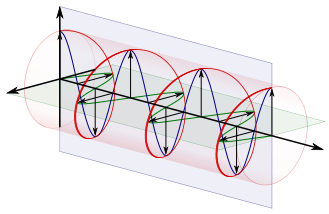
We know what that does: it ensures our wavefunction is being ‘contained’ in some ‘envelope’. It becomes a wavetrain, or a kind of beat note, as illustrated below:

[The animation comes from Wikipedia, and shows the difference between the group and phase velocity: the green dot shows the group velocity, while the red dot travels at the phase velocity.]
So… OK. That should be clear enough. Let’s now apply these thoughts to our ‘reduced’ wavefunction
Φ(φ) = a·e−iφ = a·e−i(t − β·x)
Thinking about uncertainty
Frankly, I tried to fool you above. If the functional form of the wavefunction is a·e−(i/ħ)·(E·t − p·x), then we can measure E and p in whatever unit we want, including h or ħ, but we cannot re-scale the argument of the function, i.e. the phase θ, without changing the functional form itself. I explained that in that post for my kids on wavefunctions:, in which I explained we may represent the same electromagnetic wave by two different functional forms:
F(ct−x) = G(t−x/c)
So F and G represent the same wave, but they are different wavefunctions. In this regard, you should note that the argument of F is expressed in distance units, as we multiply t with the speed of light (so it’s like our time unit is 299,792,458 m now), while the argument of G is expressed in time units, as we divide x by the distance traveled in one second). But F and G are different functional forms. Just do an example and take a simple sine function: you’ll agree that sin(θ) ≠ sin(θ/c) for all values of θ, except 0. Re-scaling changes the frequency, or the wavelength, and it does so quite drastically in this case. 🙂 Likewise, you can see that a·e−i(φ/E) = [a·e−iφ]1/E, so that’s a very different function. In short, we were a bit too adventurous above. Now, while we can drop the 1/ħ in the a·e−(i/ħ)·(E·t − p·x) function when measuring energy and momentum in units that are numerically equal to ħ, we’ll just revert to our original wavefunction for the time being, which equals
Ψ(θ) = a·e−iθ = a·e−i·[(E/ħ)·t − (p/ħ)·x]
Let’s now introduce uncertainty once again. The simplest situation is that we have two closely spaced energy levels. In theory, the difference between the two can be as small as ħ, so we’d write: E = E0 ± ħ/2. [Remember what I said about the ± A: it means the difference is 2A.] However, we can generalize this and write: E = E0 ± n·ħ/2, with n = 1, 2, 3,… This does not imply any greater uncertainty – we still have two states only – but just a larger difference between the two energy levels.
Let’s also simplify by looking at the ‘time part’ of our equation only, i.e. a·e−i·(E/ħ)·t. It doesn’t mean we don’t care about the ‘space part’: it just means that we’re only looking at how our function varies in time and so we just ‘fix’ or ‘freeze’ x. Now, the uncertainty is in the energy really but, from a mathematical point of view, we’ve got an uncertainty in the argument of our wavefunction, really. This uncertainty in the argument is, obviously, equal to:
(E/ħ)·t = [(E0 ± n·ħ/2)/ħ]·t = (E0/ħ ± n/2)·t = (E0/ħ)·t ± (n/2)·t
So we can write:
a·e−i·(E/ħ)·t = a·e−i·[(E0/ħ)·t ± (1/2)·t] = a·e−i·[(E0/ħ)·t]·ei·[±(n/2)·t]
This is valid for any value of t. What the expression says is that, from a mathematical point of view, introducing uncertainty about the energy is equivalent to introducing uncertainty about the wavefunction itself. It may be equal to a·e−i·[(E0/ħ)·t]·ei·(n/2)·t, but it may also be equal to a·e−i·[(E0/ħ)·t]·e−i·(n/2)·t. The phases of the e−i·t/2 and ei·t/2 factors are separated by a distance equal to t.
So… Well…
[…]
Hmm… I am stuck. How is this going to lead me to the ΔE·Δt = ħ/2 principle? To anyone out there: can you help? 🙂
[…]
The thing is: you won’t get the Uncertainty Principle by staring at that formula above. It’s a bit more complicated. The idea is that we have some distribution of the observables, like energy and momentum, and that implies some distribution of the associated frequencies, i.e. ω for E, and k for p. The Wikipedia article on the Uncertainty Principle gives you a formal derivation of the Uncertainty Principle, using the so-called Kennard formulation of it. You can have a look, but it involves a lot of formalism—which is what I wanted to avoid here!
I hope you get the idea though. It’s like statistics. First, we assume we know the population, and then we describe that population using all kinds of summary statistics. But then we reverse the situation: we don’t know the population but we do have sample information, which we also describe using all kinds of summary statistics. Then, based on what we find for the sample, we calculate the estimated statistics for the population itself, like the mean value and the standard deviation, to name the most important ones. So it’s a bit the same here, except that, in quantum mechanics, there may not be any real value underneath: the mean and the standard deviation represent something fuzzy, rather than something precise.
Hmm… I’ll leave you with these thoughts. We’ll develop them further as we will be digging into all much deeper over the coming weeks. 🙂
Post scriptum: I know you expect something more from me, so… Well… Think about the following. If we have some uncertainty about the energy E, we’ll have some uncertainty about the momentum p according to that β = p/E. [By the way, please think about this relationship: it says, all other things being equal (such as the inertia, i.e. the mass, of our particle), that more energy will all go into more momentum. More specifically, note that ∂p/∂p = β according to this equation. In fact, if we include the mass of our particle, i.e. its inertia, as potential energy, then we might say that (1−β)·E is the potential energy of our particle, as opposed to its kinetic energy.] So let’s try to think about that.
Let’s denote the uncertainty about the energy as ΔE. As should be obvious from the discussion above, it can be anything: it can mean two separate energy levels E = E0 ± A, or a potentially infinite set of values. However, even if the set is infinite, we know the various energy levels need to be separated by ħ, at least. So if the set is infinite, it’s going to be a countable infinite set, like the set of natural numbers, or the set of integers. But let’s stick to our example of two values E = E0 ± A only, with A = ħ so E + ΔE = E0 ± ħ and, therefore, ΔE = ± ħ. That implies Δp = Δ(β·E) = β·ΔE = ± β·ħ.
Hmm… This is a bit fishy, isn’t it? We said we’d measure the momentum in units of ħ, but so here we say the uncertainty in the momentum can actually be a fraction of ħ. […] Well… Yes. Now, the momentum is the product of the mass, as measured by the inertia of our particle to accelerations or decelerations, and its velocity. If we assume the inertia of our particle, or its mass, to be constant – so we say it’s a property of the object that is not subject to uncertainty, which, I admit, is a rather dicey assumption (if all other measurable properties of the particle are subject to uncertainty, then why not its mass?) – then we can also write: Δp = Δ(m·v) = Δ(m·β) = m·Δβ. [Note that we’re not only assuming that the mass is not subject to uncertainty, but also that the velocity is non-relativistic. If not, we couldn’t treat the particle’s mass as a constant.] But let’s be specific here: what we’re saying is that, if ΔE = ± ħ, then Δv = Δβ will be equal to Δβ = Δp/m = ± (β/m)·ħ. The point to note is that we’re no longer sure about the velocity of our particle. Its (relative) velocity is now:
β ± Δβ = β ± (β/m)·ħ
But, because velocity is the ratio of distance over time, this introduces an uncertainty about time and distance. Indeed, if its velocity is β ± (β/m)·ħ, then, over some time T, it will travel some distance X = [β ± (β/m)·ħ]·T. Likewise, it we have some distance X, then our particle will need a time equal to T = X/[β ± (β/m)·ħ].
You’ll wonder what I am trying to say because… Well… If we’d just measure X and T precisely, then all the uncertainty is gone and we know if the energy is E0 + ħ or E0 − ħ. Well… Yes and no. The uncertainty is fundamental – at least that’s what’s quantum physicists believe – so our uncertainty about the time and the distance we’re measuring is equally fundamental: we can have either of the two values X = [β ± (β/m)·ħ] T = X/[β ± (β/m)·ħ], whenever or wherever we measure. So we have a ΔX and ΔT that are equal to ± [(β/m)·ħ]·T and X/[± (β/m)·ħ] respectively. We can relate this to ΔE and Δp:
- ΔX = (1/m)·T·Δp
- ΔT = X/[(β/m)·ΔE]
You’ll grumble: this still doesn’t give us the Uncertainty Principle in its canonical form. Not at all, really. I know… I need to do some more thinking here. But I feel I am getting somewhere. 🙂 Let me know if you see where, and if you think you can get any further. 🙂
The thing is: you’ll have to read a bit more about Fourier transforms and why and how variables like time and energy, or position and momentum, are so-called conjugate variables. As you can see, energy and time, and position and momentum, are obviously linked through the E·t and p·x products in the E0·t − p·x sum. That says a lot, and it helps us to understand, in a more intuitive way, why the ΔE·Δt and Δp·Δx products should obey the relation they are obeying, i.e. the Uncertainty Principle, which we write as ΔE·Δt ≥ ħ/2 and Δp·Δx ≥ ħ/2. But so proving involves more than just staring at that Ψ(θ) = a·e−iθ = a·e−i·[(E/ħ)·t − (p/ħ)·x] relation.
Having said, it helps to think about how that E·t − p·x sum works. For example, think about two particles, a and b, with different velocity and mass, but with the same momentum, so pa = pb ⇔ ma·va = ma·va ⇔ ma/vb = mb/va. The spatial frequency of the wavefunction would be the same for both but the temporal frequency would be different, because their energy incorporates the rest mass and, hence, because ma ≠ mb, we also know that Ea ≠ Eb. So… It all works out but, yes, I admit it’s all very strange, and it takes a long time and a lot of reflection to advance our understanding.


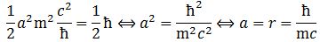
 We can write this as a function of m and the c and ħ constants only: