Electric circuits (1): the circuit elements

OK. No escape. It’s part of physics. I am not going to go into the nitty-gritty of it all (because this is a blog about physics, not about engineering) but it’s good to review the basics, which are, essentially, Kirchoff’s rules. Just for the record, Gustav Kirchhoff was a German genius who formulated these circuit laws while he was still a student, when he was like 20 years old or so. He did it as a seminar exercise 170 years ago, and then turned it into doctoral dissertation. Makes me think of that Dire Straits song—That’s the way you do it—Them guys ain’t dumb. 🙂

So this post is, in essence, just an ‘explanation’ of Feynman’s presentation of Kirchoff’s rules, so I am writing this post basically for myself, so as to ensure I am not missing anything. To be frank, Feynman’s use of notation when working with complex numbers is confusing at times and so, yes, I’ll do some ‘re-writing’ here. The nice thing about Feynman’s presentation of electrical circuits is that he sticks to Maxwell’s Laws when describing all ideal circuit elements, so he keeps using line integrals of the electric field E around closed paths (that’s what a circuit is, indeed) to describe the so-called passive circuit elements, and he also recapitulates the idea of the electromotive force when discussing the so-called active circuit element, so that’s the generator. That’s nice, because it links it all with what we’ve learned so far, i.e. the fundamentals as expressed in Maxwell’s set of equations. Having said that, I won’t make that link here in this post, because I feel it makes the whole approach rather heavy.

OK. Let’s go for it. Let’s first recall the concept of impedance.

The impedance concept

There are three ideal (passive) circuit elements: the resistor, the capacitor and the inductor. Real circuit elements usually combine characteristics of all of them, even if they are designed to work like ideal circuit elements. Collectively, these ideal (passive) circuit elements are referred to as impedances, because… Well… Because they have some impedance. In fact, you should note that, if we reserve the terms ending with -ance for the property of the circuit elements, and those ending on -or for the objects themselves, then we should call them impedors. However, that term does not seem to have caught on.

You already know what impedance is. I explained it before, notably in my post on the intricacies related to self- and mutual inductance. Impedance basically extends the concept of resistance, as we know it from direct current (DC) circuits, to alternating current (AC) circuits. To put it simply, when AC currents are involved – so when the flow of charge periodically changes reverses direction – then it’s likely that, because of the properties of the circuit, the current signal will lag the voltage signal, and so we’ll have some phase difference telling us by how much. So, resistance is just a simple real number R – it’s the ratio between (1) the voltage that is being applied across the resistor and (2) the current through it, so we write R = V/I – and it’s got a magnitude only, but impedance is a ‘number’ that has both a magnitude as well as phase, so it’s a complex number, or a vector.

In engineering, such ‘numbers’ with a magnitude as well as a phase are referred to as phasors. A phasor represents voltages, currents and impedances as a phase vector (note the bold italics: they explain how we got the pha-sor term). It’s just a rotating vector really. So a phasor has a varying magnitude (A) and phase (φ) , which is determined by (1) some maximum magnitude A₀, (2) some angular frequency ω and (3) some initial phase (θ). So we can write the amplitude A as:

A = A(φ) = A₀·cos(φ) = A₀·cos(ωt + θ)

As usual, Wikipedia has a nice animation for it:

In case you wonder why I am using a cosine rather than a sine function, the answer is that it doesn’t matter: the sine and the cosine are the same function except for a π/2 phase difference: just rotate the animation above by 90 degrees, or think about the formula: sinφ = cos(φ−π/2). 🙂

So A = A₀·cos(ωt + θ) is the amplitude. It could be the voltage, or the current, or whatever real variable. The phase vector itself is represented by a complex number, i.e. a two-dimensional number, so to speak, which we can write as all of the following:

A = A₀·e^iφ = A₀·cosφ + i·A₀·sinφ = A₀·cos(ωt+θ) + i·A₀·sin(ωt+θ)

= A₀·e^i(ωt+θ)= A₀·e^iθ·e^iωt= A₀·e^iωtwith A₀= A₀·e^iθ

That’s just Euler’s formula, and I am afraid I have to refer you to my page on the essentials if you don’t get this. I know what you are thinking: why do we need the vector notation? Why can’t we just be happy with the A = A₀·cos(ωt+θ) formula? The truthful answer is: it’s just to simplify calculations: it’s easier to work with exponentials than with cosines or sines. For example, writing e^{i(ωt + θ)}= e^iθ·e^iωtis easier than writing cos(ωt + θ) = … […] Well? […] Hmm… 🙂

See! You’re stuck already. You’d have to use the cos(α+β) = cosα·cosβ − sinα·sinβ formula: you’d get the same results (just do it for the simple calculation of the impedance below) but it takes a lot more time, and it’s easier to make mistake. Having said why complex number notation is great, I also need to warn you. There are a few things you have to watch out for. One of these things is notation. The other is the kind of mathematical operations we can do: it’s usually alright but we need to watch out with the i² = –1 thing when multiplying complex numbers. However, I won’t talk about that here because it would only confuse you even more. 🙂

Just for the notation, let me note that Feynman would write A₀as A₀ with the little hat or caret symbol (∧) on top of it, so as to indicate the complex coefficient is not a variable. So he writes A₀as Â₀ = A₀·e^iθ. However, I find that confusing and, hence, I prefer using bold-type for any complex number, variable or not. The disadvantage is that we need to remember that the coefficient in front of the exponential is not a variable: it’s a complex number alright, but not a variable. Indeed, do look at that A₀= A₀·e^iθ equality carefully: A₀is a specific complex number that captures the initial phase θ. So it’s not the magnitude of the phasor itself, i.e. |A| = A₀. In fact, magnitude, amplitude, phase… We’re using a lot confusing terminology here, and so that’s why you need to ‘get’ the math.

The impedance is not a variable either. It’s some constant. Having said that, this constant will depend on the angular frequency ω. So… Well… Just think about this as you continue to read. 🙂 So the impedance is some number, just like resistance, but it’s a complex number. We’ll denote it by Z and, using Euler’s formula once again, we’ll write it as:

Z = |Z|eⁱ^θ= V/I = |V|eⁱ^{(ωt +}^θ_V⁾/|I|eⁱ^{(ωt +}^θ_I⁾= [|V|/|I|]·eⁱ⁽^θ_V⁻^θ_I⁾

So, as you can see, it is, literally, some complex ratio, just like R = V/I was some real ratio: it is a complex ratio because it has a magnitude and a direction, obviously. Also please do note that, as I mentioned already, the impedance is, in general, some function of the frequency ω, as evidenced by the ωt term in the exponential, but so we’re not looking at ω as a variable: V and I are variables and, as such, they depend on ω, but so you should look at ω as some parameter. I know I should, perhaps, not be so explicit on what’s going on, but I want to make sure you understand.

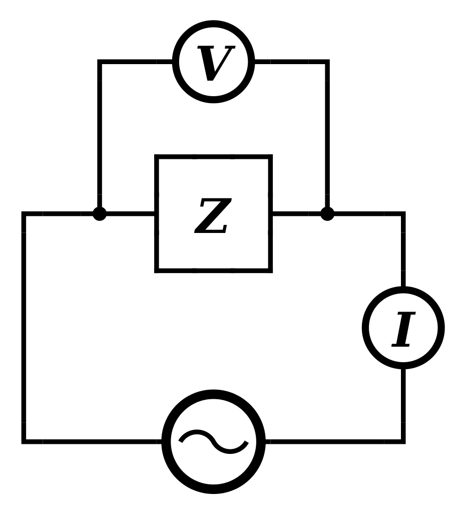
So what’s going on? The illustration below (credit goes to Wikipedia, once again) explains. It’s a pretty generic view of a very simple AC circuit. So we don’t care what the impedance is: it might be an inductor or a capacitor, or a combination of both, but we don’t care: we just call it an impedance, or an impedor if you want. 🙂 The point is: if we apply an alternating current, then the current and the voltage will both go up and down, but the current signal will lag the voltage signal, and some phase factor θ tells us by how much, so θ will be the phase difference.

Now, we’re dividing one complex number by another in that Z = V/I formula above, and dividing one complex number by another is not all that straightforward, so let me re-write that formula for Z above as:

V = I∗Z = I∗|Z|eⁱ^θ

Now, while that V = I∗Z formula resembles the V = I·R formula, you should note the bold-face type for V and I, and the ∗ symbol I am using here for multiplication. The bold-face for V and I implies they’re vectors, or complex numbers. As for the ∗ symbol, that’s to make it clear we’re not talking a vector cross product A×B here, but a product of two complex numbers. [It’s obviously not a vector dot product either, because a vector dot product yields a real number, not some other vector.]

Now we write V and I as you’d expect us to write them:

V = |V|eⁱ^{(ωt +}^θ_V⁾= V₀·eⁱ^{(ωt +}^θ_V⁾
I = |I|eⁱ^{(ωt +}^θ_I⁾= I₀·eⁱ^{(ωt +}^θ_I⁾

θ_V and θ_Iare, obviously, the so-called initial phase of the voltage and the current respectively. These ‘initial’ phases are not independent: we’re talking a phase difference really, between the voltage and the current signal, and it’s determined by the properties of the circuit. In fact, that’s the whole point here: the impedance is a property of the circuit and determines how the current signal varies as a function of the voltage signal. In fact, we’ll often choose the t = 0 point such that θ_Vand so then we need to find θ_I. […] OK. Let’s get on with it. Writing out all of the factors in the V = I∗Z = I∗|Z|eⁱ^θ equation yields:

V = |V|eⁱ^{(ωt +}^θ_V⁾= I∗Z = |I|eⁱ^{(ωt +}^θ_I⁾∗|Z|eⁱ^θ= |I||Z|eⁱ^{(ωt +}^θ_I^+ θ)

Now, this equation must hold for all values of t, so we can equate the magnitudes and phases and, hence, the following equalities must hold:

|V| = |I||Z| ⇔ |Z| = |V|/|I|
ωt + θ_V = ωt + θ_I+ θ ⇔ θ = θ_V − θ_I

Done!

Of course, you’ll complain once again about those complex numbers: voltage and current are something real, isn’t it? And so what is really about this complex numbers? Well… I can just say what I said already. You’re right. I’ve used the complex notation only to simplify the calculus, so it’s only the real part of those complex-valued functions that counts.

OK. We’re done with impedance. We can now discuss the impedors, including resistors (for which we won’t have such lag or phase difference, but the concept of impedance applies nevertheless).

Before I start, however, you should think about what I’ve done above: I explained the concept of impedance, but I didn’t do much with it. The real-life problem will usually be that you get the voltage as a function of time, and then you’ll have to calculate the impedance of a circuit and, then, the current as a function of time. So I just showed the fundamental relations but, in real life, you won’t know what θ and θ_I could possibly be. Well… Let me correct that statement: we’ll give you formulas for θ as we discuss the various circuit elements and their impedance below, and so then you can use these formulas to calculate θ_I. 🙂

Resistors

Let’s start with what seems to be the easiest thing: a resistor. A real resistor is actually not easy to understand, because it requires us to understand the properties of real materials. Indeed, it may or may not surprise you, but the linear relation between the voltage and the current for real materials is only approximate. Also, the way resistors dissipate energy is not easy to understand. Indeed, unlike inductors and capacitors, i.e. the other two passive components of an electrical circuit, a resistor does not store but dissipates energy, as shown below.

It’s a nice animation (credit for it has to go to Wikipedia once more), as it shows how energy is being used in an electric circuit. Note that the little moving pluses are in line with the convention that a current is defined as the movement of positive charges, so we write I = dQ/dt instead of I = −dQ/dt. That also explains the direction of the field line E, which has been added to show that the charges move with the field that is being generated by the power source (which is not shown here). So, what we have here is that, on one side of the circuit, some generator or voltage source will create an emf pushing the charges, and so the animation shows how some load – i.e. the resistor in this case – will consume their energy, so they lose their push (as shown by the change in color from yellow to black). So power, i.e.energy per unit time, is supplied, and is then consumed.

To increase the current in the circuit above, you need to increase the voltage, but increasing both amounts to increasing the power that’s being consumed in the circuit. Electric power is voltage times current, so P = V·I (or v·i, if I use the small letters that are used in the two animations below). Now, Ohm’s Law (I = V/R) says that, if we’d want to double the current, we’d need to double the voltage, and so we’re quadrupling the power then: P₂ = V₂·I₂= (2·V₁)·(2·I₁) = 4·V₁·I₁= 2²·P₁. So we have a square-cube law for the power, which we get by substituting V for R·I or by substituting I for V/R, so we can write the power P as P = V²/R = I²·R. This square-cube law says exactly the same: if you want to double the voltage or the current, you’ll actually have to double both and, hence, you’ll quadruple the power.

But back to the impedance: Ohm’s Law is the Z = V/I law for resistors, but we can simplify it because we know the voltage across the resistor and the current that’s going through are in phase. Hence, θ_V and θ_Iare identical and, therefore, the θ = θ_V− θ_Iin Z = |Z|eⁱ^θis equal to zero and, hence, Z = |Z|. Now, |Z| = |V|/|I| = V₀/I₀. So the impedance Z is just some real number R = V₀/I₀, which we can also write as:

R = V₀/I₀= (V₀·eⁱ^{(ωt + α}⁾)/(I₀·eⁱ^{(ωt + α}⁾) = V(t)/I(t), with α = θ_V = θ_I

The equation above goes from R = V₀/I₀to R = V(t)/I(t) = V/I. It’s note the same thing: the second equation says that, at any point in time, the voltage and the current will be proportional to each other, with R or its reciprocal as the proportionality constant. In any case, we have our formula for Z here:

Z = R = V/I = V₀/I₀

So that’s simple. Before we move to the next, let me note that the resistance of a real resistor may depend on its temperature, so in real-life applications one will want to keep its temperature as stable as possible. That’s why real-life resistors have power ratings and recommended operating temperatures. The image below illustrates how so-called heat-sink resistors can be mounted on a heat sink with a simple spring clip so as to ensure the dissipated heat is transported away. These heat-sink resistors are rather small (10 by 15 mm only) but are rated for 35 watt – so that’s quite a lot for such small thing – if correctly mounted.

As mentioned, the linear relation between the voltage and the current is only approximate, and the observed relation is also there only for frequencies that are not ‘too high’ because, if the frequency becomes very high, the free electrons will start radiating energy away, as they produce electromagnetic radiation. So one always needs to look at the tolerances of real-life resistors, which may be ± 5%, ± 10%, or whatever. In any case… On to the next.

Capacitors (condensers)

We talked at length about capacitors (aka condensers) in our post explaining capacitance or, the more widely used term, capacity: the capacity of a capacitor is the observed proportionality between (1) the voltage (V) across and (2) the charge (Q) on the capacitor, so we wrote it as:

C = Q/V

Now, it’s easy to confuse the C here with the C for coulomb, which I’ll also use in a moment, and so… Well… Just don’t! 🙂 The meaning of the symbol is usually obvious from the context.

As for the explanation of this relation, it’s quite simple: a capacitor consists of two separate conductors in space, with positive charge on one, and an equal and opposite (i.e. negative) charge on the other. Now, the logic of the superposition of fields implies that, if we double the charges, we will also double the fields, and so the work one needs to do to carry a unit charge from one conductor to the other is also doubled! So that’s why the potential difference between the conductors is proportional to the charge.

The C = Q/V formula actually measures the ability of the capacitor to store electric charge and, therefore, to store energy, so that’s why the term capacity is really quite appropriate. I’ll let you google a few illustrations like the one below, that shows how a capacitor is actually being charged in a circuit. Usually, some resistance will be there in the circuit, so as to limit the current when it’s connected to the voltage source and, therefore, as you can see, the R times C factor (R·C) determines how fast or how slow the capacitor charges and/or discharges. Also note that the current is equal to the time rate of change of the charge: I = dQ/dt.

In the above-mentioned post, we also give a few formulas for the capacity of specific types of condensers. For example, for a parallel-plate condenser, the formula was C = ε₀A/d. We also mentioned its unit, which is is coulomb/volt, obviously, but – in honor of Michael Faraday, who gave us Faraday’s Law, and many other interesting formulas – it’s referred to as the farad: 1 F = 1 C/V. The C here is coulomb, of course. Sorry we have to use C to denote two different things but, as I mentioned, the meaning of the symbol is usually clear from the context.

We also talked about how dielectrics actually work in that post, but we did not talk about the impedance of a capacitor, so let’s do that now. The calculation is pretty straightforward. Its interpretation somewhat less so. But… Well… Let’s go for it.

It’s the current that’s charging the condenser (sorry I keep using both terms interchangeably), and we know that the current is the time rate of change of the charge (I = dQ/dt). Now, you’ll remember that, in general, we’d write a phasor A as A = A₀·e^iωtwith A₀= A₀·e^iθ, so A₀is a complex coefficient incorporating the initial phase, which we wrote as θ_Vand θ_Ifor the voltage and for the current respectively. So we’ll represent the voltage and the current now using that notation, so we write: V = V₀·e^iωtand I = I₀·e^iωt. So let’s now use that C = Q/V by re-writing it as Q = C·V and, because C is some constant, we can write:

I = dQ/dt = d(C·V)/dt = C·dV/dt

Now, what’s dV/dt? Oh… You’ll say: V is the magnitude of V, so it’s equal to |V| = |V₀·e^iωt| = |V₀|·|e^iωt| = |V₀| = |V₀·e^iθ| = |V₀|·|e^iθ| = |V₀| = V₀. So… Well… What? V₀ is some constant here! It’s the maximum amplitude of V, so… Well… It’s time derivative is zero: dV₀/dt = 0.

Yes. Indeed. We did something very wrong here! You really need to watch out with this complex-number notation, and you need to think about what you’re doing. V is not the magnitude of V but its (varying) amplitude. So it’s the real voltage V that varies with time: it’s equal to V₀·cos(ωt + θ_V), which is the real part of our phasor V. Huh? Yes. Just hang in for a while. I know it’s difficult and, frankly, Feynman doesn’t help us very much here. Let’s take one step back and so – you will see why I am doing this in a moment – let’s calculate the time derivative of our phasor V, instead of the time derivative of our real voltage V. So we calculate dV/dt, which is equal to:

dV/dtd(V₀·e^iωt)/dt = V₀·d(e^iωt)/dt = V₀·(iω)·e^iωt = iω·V₀·e^iωt = iω·V

Remarkable result, isn’t it? We take the time derivative of our phasor, and the result is the phasor itself multiplied with iω. Well… Yes. It’s a general property of exponentials, but still… Remarkable indeed! We’d get the same with I, but we don’t need that for the moment. What we do need to do is go from our I = C·dV/dt relation, which connects the real parts of I and V one to another, to the I = C·dV/dt relation, which relates the (complex) phasors. So we write:

I = C·dV/dt ⇔ I = C·dV/dt

Can we do that? Just like that? We just replace I and V by I and V? Yes, we can. Why? Well… We know that I is the real part of I and so we can write I = Re(I)+ Im(I)·i = I + Im(I)·i, and then we can write the right-hand side of the equation as C·dV/dt = Re(C·dV/dt)+ Im(C·dV/dt)·i. Now, two complex numbers are equal if, and only if, their real and imaginary parts are the same, so… Well… Write it all out, if you want, using Euler’s formula, and you’ll see it all makes sense indeed.

So what do we get? The I = C·dV/dt gives us:

I = C·dV/dt = C·(iω)·V

That implies that I/V = C·(iω) and, hence, we get – finally! – what we need to get:

Z = V/I = 1/(iωC)

This is a grand result and, while I am sorry I made you suffer for it, I think it did a good job here because, if you’d check Feynman on it, you’ll see he – or, more probably, his assistants, – just skate over this without bothering too much about mathematical rigor. OK. All that’s left now is to interpret this ‘number’ Z = 1/(iωC). It is a purely imaginary number, and it’s a constant indeed, albeit a complex constant. It can be re-written as:

Z = 1/(iωC) = i^-1/(ωC) = –i/(ωC) = (1/ωC)·e^−i·π/2

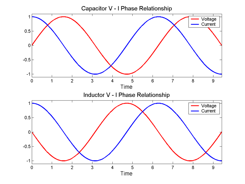
[Sorry. I can’t be more explicit here. It’s just of the wonders of complex numbers: i^-1= –i. Just check one my posts on complex numbers for more detail.] Now, a –i factor corresponds to a rotation of minus 90 degrees, and so that gives you the true meaning of what’s usually said about a circuit with a capacitor: the voltage across the capacitor will lag the current with a phase difference equal to π/2, as shown below. Of course, as it’s the voltage driving the current, we should say it’s the current that is lagging with a phase difference of 3π/2, rather than stating it the other way around! Indeed, i^-1= –i = –1·i = i²·i = i³, so that amounts to three ‘turns’ of the phase in the counter-clockwise direction, which is the direction in which our ωt angle is ‘turning’.

It is a remarkable result, though. The illustration above assumes the maximum amplitude of the voltage and the current are the same, so |Z| = |V|/|I| = 1, but what if they are not the same? What are the real bits then? I can hear you, indeed: “To hell with the bold-face letters: what’s V and I? What’s the real thing?”

Well… V and I are the real bits of V = |V|eⁱ^(ωt+^θ_V⁾= V₀·eⁱ^(ωt+^θ_V⁾and of I = |I|eⁱ^(ωt+^θ_I⁾= I₀·eⁱ^{(ωt+θ_V−θ}⁾ = I₀·eⁱ^(ωt−^θ⁾= I₀·eⁱ^(ωt+^π/2⁾respectively so, assuming θ_V= 0 (as mentioned above, that’s just a matter of choosing a convenient t = 0 point), we get:

V = V₀·cos(ωt)
I = I₀·cos(ωt + π/2)

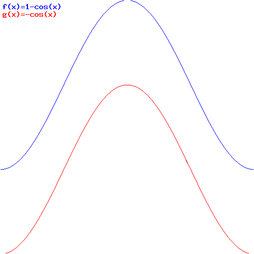
So the π/2 phase difference is there (you need to watch out with the signs, of course: θ = −π/2, but so it’s the current that seems to lead here) but the V₀/I₀ratio doesn’t have to be one, so the real voltage and current could look like something below, where the maximum amplitude of the current is only half of the maximum amplitude of the voltage.

So let’s analyze this quickly: the V₀/I₀ratio is equal to |Z| = |V|/|I| = V₀/I₀= 1/ωC = (1/ω)(1/C) (note that it’s not equal to V/I = V(t)/I(t), which is a ratio that doesn’t make sense because I(t) goes through zero as the current switches direction). So what? Well… It means the ratio is inversely proportional to both the frequency ω as well as the capacity C, as shown below. Think about this: if ω goes to zero, V₀/I₀goes to ∞, which means that, for a given voltage, the current must go to zero. That makes sense, because we’re talking DC current when ω → 0, and the capacitor charges itself and then that’s it: no more currents. Now, if C goes to zero, so we’re talking capacitors with hardly any capacity, we’ll also get tiny currents. Conversely, for large C, we’ll get huge currents, as the capacitor can take pretty much any charge you throw at it, so that makes for small V₀/I₀ratios. The most interesting thing to consider is ω going to infinity, as the V₀/I₀ratio is also quite small then. What happens? The capacitor doesn’t get the time to charge, and so it’s always in this state where it has large currents flowing in and out of it, as it can’t build the voltage that would counter the electromotive force that’s being supplied by the voltage source.

OK. That’s it. Le’s discuss the last (passive) element.

Inductors

We’ve spoiled the party a bit with that illustration above, as it gives the phase difference for an inductor already:

Z = iωL = ωL·e^i·π/2, with L the inductance of the coil

So, again assuming that θ_V= 0, we can calculate I as:

I = |I|eⁱ^(ωt+^θ_I⁾= I₀·eⁱ^{(ωt+θ_V−θ}⁾ = I₀·eⁱ^(ωt−^θ⁾= I₀·eⁱ^(ωt−^π/2⁾

Of course, you’ll want to relate this, once again, to the real voltage and the real current, so let’s write the real parts of our phasors:

V = V₀·cos(ωt)
I = I₀·cos(ωt − π/2)

Just to make sure you’re not falling asleep as you’re reading, I’ve made another graph of how things could look like. So now’s it’s the current signal that’s lagging the voltage signal with a phase difference equal to θ = π/2.

Also, to be fully complete, I should show you how the V₀/I₀ratio now varies with L and ω. Indeed, here also we can write that |Z| = |V|/|I| = V₀/I₀, but so here we find that V₀/I₀ = ωL, so we have a simple linear proportionality here! For example, for a given voltage V₀, we’ll have smaller currents as ω increases, so that’s the opposite of what happens with our ideal capacitors. I’ll let you think about that… 🙂

Now how do we get that Z = iωL formula? In my post on inductance, I explained what an inductor is: a coil of wire, basically. Its defining characteristic is that a changing current will cause a changing magnetic field in it and, hence, some change in the flux of the magnetic field. Now, Faraday’s Law tells us that that will cause some circulation of the electric field in the coil, which amounts to an induced potential difference which is referred to as the electromotive force (emf). Now, it turns out that the induced emf is proportional to the change in current. So we’ve got another constant of proportionality here, so it’s like how we defined resistance, or capacitance. So, in many ways, the inductance is just another proportionality coefficient. If we denote it by L – the symbol is said to honor the Russian phyicist Heinrich Lenz, whom you know from Lenz’ Law – then we define it as:

L = −Ɛ/(dI/dt)

The dI/dt factor is, obviously, the time rate of change of the current, and the negative sign indicates that the emf opposes the change in current, so it will tend to cause an opposing current. However, the power of our voltage source will ensure the current does effectively change, so it will counter the ‘back emf’ that’s being generated by the inductor. To be precise, the voltage across the terminals of our inductor, which we denote by V, will be equal and opposite to Ɛ, so we write:

V = −Ɛ = L·(dI/dt)

Now, this very much resembles the I = C·dV/dt relation we had for capacitors, and it’s completely analogous indeed: we just need to switch the I and V, and C and L symbols. So we write:

V = L·dI/dt⇔ V = L·dI/dt

Now, dI/dt is a similar time derivative as dV/dt. We calculate it as:

dI/dtd(I₀·e^iωt)/dt = I₀·d(e^iωt)/dt = I₀·(iω)·e^iωt = iω·I₀·e^iωt = iω·I

So we get what we want and have to get:

V = L·dI/dt = iωL·I

Now, Z = V/I, so Z = iωL indeed!

Summary of conclusions

Let’s summarize what we found:

For a resistor, we have Z(resistor) = Z_R= R = V/I = V₀/I₀
For an capacitor, we have Z(capacitor) = Z_C= 1/(iωC) = –i/(ωC)
For an inductor, we have Z(inductance) = Z_L= iωL

Note that the impedance of capacitors decreases as frequency increases, while for inductors, it’s the other way around. We explained that by making you think of the currents: for a given voltage, we’ll have large currents for high frequencies, and, hence, a small V₀/I₀ratio. Can you think of what happens with an inductor? It’s not so easy, so I’ll refer you to the addendum below for some more explanation.

Let me also note that, as you can see, the impedance of (ideal) inductors and capacitors is a pure imaginary number, so that’s a complex number which has no real part. In engineering, the imaginary part of the impedance is referred to as the reactance, so engineers will say that ideal capacitors and inductors have a purely imaginary reactive impedance.

However, in real life, the impedance will usually have both a real as well as an imaginary part, so it will be some kind of mix, so to speak. The real part is referred to as the ‘resistance’ R, and the ‘imaginary’ part is referred to as the ‘reactance’ X. The formula for both is given below:

But here I have to end my post on circuit elements. It’s become quite long, so I’ll discuss Kirchoff’s rules in my next post.

Addendum: Why is V = − Ɛ?

Inductors are not easy to understand—intuitively, that is. That’s why I spent so much time writing on them in my other post on them, to which I should be referring you here. But let me recapitulate the key points. The key idea is that we’re pumping energy into an inductor when applying a current and, as you know, the time rate of change is power: P = dW/dt, so we’re talking power here too, which is voltage times current: P = dW/dt = V·I. The illustration below shows what happens when an alternating current is applied to the circuit with the inductor. So the assumption is that the current goes in one and then in the other direction, so I > 0, and then I < 0, etcetera. We’re also assuming some nice sinusoidal curve for the current here (i.e. the blue curve), and so we get what we get for U (i.e. the red curve), which is the energy that’s stored in the inductor really, as it tries to resist the changing current: the energy goes up and down between zero and some maximum amplitude that’s determined by the maximum current.

So, yes, building up current requires energy from some external source, which is used to overcome the ‘back emf’ in the inductor, and that energy is stored in the inductor itself. [If you still wonder why it’s stored in the inductor, think about the other question: where else would it be stored?] How is stored? Look at the graph and think: it’s stored as kinetic energy of the charges, obviously. That explains why the energy is zero when the current is zero, and why the energy maxes out when the current maxes out. So, yes, it all makes sense! 🙂

Let me give another example. The graph below assumes the current builds up to some maximum. As it reaches its maximum, the stored energy will also max out. This example assumes direct current, so it’s a DC circuit: the current builds up, but then stabilizes at some maximum that we can find by applying Ohm’s Law to the resistance of the circuit: I = V/R. Resistance? But we were talking an ideal inductor? We are. If there’s no other resistance in the circuit, we’ll have a short-circuit, so the assumption is that we do have some resistance in the circuit and, therefore, we should also think of some energy loss to heat from the current in the resistance. If not, well… Your power source will obviously soon reach its limits. 🙂

So what’s going on then? We have some changing current in the coil but, obviously, some kind of inertia also: the coil itself opposes the change in current through the ‘back emf’. Now, it requires energy, or power, to overcome the inertia, so that’s the power that comes from our voltage source: it will offset the ‘back emf’, so we may effectively think of a little circuit with an inductor and a voltage source, as shown below.

But why do we write V = − Ɛ? Our voltage source can have any voltage, can’t it? Yes. Sure. But so the coil will always provide an emf that’s exactly the opposite of this voltage. Think of it: we have some voltage that’s being applied across the terminals of the inductor, and so we’ll have some current. A current that’s changing. And it’s that current will generate an emf that’s equal to Ɛ = –L·(dI/dt). So don’t think of Ɛ as some constant: it’s the self-inductance coefficient L that’s constant, but I (and, hence, dI/dt) and V are variable.

The point is: we cannot have any potential difference in a perfect conductor, which is what the terminals are: any potential difference, i.e. any electric field really, would cause huge currents. In other words, the voltage V and the emf Ɛ have to cancel each other out, all of the time. If not, we’d have huge currents in the wires re-establishing the V = −Ɛ equality.

Let me use Feynman’s argument here. Perhaps that will work better. 🙂 Our ideal inductor is shown below: it’s shielded by some metal box so as to ensure it does not interact with the rest of the circuit. So we have some current I, which we assume to be an AC current, and we know some voltage is needed to cause that current, so that’s the potential difference V between the terminals.

The total circulation of E – around the whole circuit – can be written as the sum of two parts:

Now, we know circulation of E can only be caused by some changing magnetic field, which is what’s going on in the inductor:

So this change in the magnetic flux is what it causing the ‘back emf’, and so the integral on the left is, effectively, equal to Ɛ, not minus Ɛ but +Ɛ. Now, the second integral is equal to V, because that’s the voltage V between the two terminals a and b. So the whole integral is equal to 0 = Ɛ + V and, therefore, we have that:

V = − Ɛ = L·dI/dt

Some content on this page was disabled on June 16, 2020 as a result of a DMCA takedown notice from The California Institute of Technology. You can learn more about the DMCA here:

https://en.support.wordpress.com/copyright-and-the-dmca/
Some content on this page was disabled on June 16, 2020 as a result of a DMCA takedown notice from The California Institute of Technology. You can learn more about the DMCA here:

https://en.support.wordpress.com/copyright-and-the-dmca/

An introduction to electric circuits

In my previous post,I introduced electric motors, generators and transformers. They all work because of Faraday’s flux rule: a changing magnetic flux will produce some circulation of the electric field. The formula for the flux rule is given below:

It is a wonderful thing, really, but not easy to grasp intuitively. It’s one of these equations where I should quote Feynman’s introduction to electromagnetism: “The laws of Newton were very simple to write down, but they had a lot of complicated consequences and it took us a long time to learn about them all. The laws of electromagnetism are not nearly as simple to write down, which means that the consequences are going to be more elaborate and it will take us quite a lot of time to figure them all out.”

Now, among Maxwell’s Laws, this is surely the most complicated one! However, that shouldn’t deter us. 🙂 Recalling Stokes’ Theorem helps to appreciate what the integral on the left-hand side represents:

We’ve got a line integral around some closed loop Γ on the left and, on the right, we’ve got a surface integral over some surface S whose boundary is Γ. The illustration below depicts the geometry of the situation. You know what it all means. If not, I am afraid I have to send you back to square one, i.e. my posts on vector analysis. Yep. Sorry. Can’t keep copying stuff and make my posts longer and longer. 🙂

To understand the flux rule, you should imagine that the loop Γ is some loop of electric wire, and then you just replace C by E, the electric field vector. The circulation of E, which is caused by the change in magnetic flux, is referred to as the electromotive force (emf), and it’s the tangential force (E·ds) per unit charge in the wire integrated over its entire length around the loop, which is denoted by Γ here, and which encloses a surface S.

Now, you can go from the line integral to the surface integral by noting Maxwell’s Law: −∂B/∂t = ∇×E. In fact, it’s the same flux rule really, but in differential form. As for (∇×E)_n, i.e. the component of ∇×E that is normal to the surface, you know that any vector multiplied with the normal unit vector will yield its normal component. In any case, if you’re reading this, you should already be acquainted with all of this. Let’s explore the concept of the electromotive force, and then apply it our first electric circuit. 🙂

Indeed, it’s now time for a small series on circuits, and so we’ll start right here and right now, but… Well… First things first. 🙂

The electromotive force: concept and units

The term ‘force’ in ‘electromotive force’ is actually somewhat misleading. There is a force involved, of course, but the emf is not a force. The emf is expressed in volts. That’s consistent with its definition as the circulation of E: a force times a distance amounts to work, or energy (one joule is one newton·meter), and because E is the force on a unit charge, the circulation of E is expressed in joule per coulomb, so that’s a voltage: 1 volt = 1 joule/coulomb. Hence, on the left-hand side of Faraday’s equation, we don’t have any dimension of time: it’s energy per unit charge, so it’s x joule per coulomb . Full stop.

On the right-hand side, however, we have the time rate of change of the magnetic flux. through the surface S. The magnetic flux is a surface integral, and so it’s a quantity expressed in [B]·m², with [B] the measurement unit for the magnetic field strength. The time rate of change of the flux is then, of course, expressed in [B]·m²per second, i.e. [B]·m²/s. Now what is the unit for the magnetic field strength B, which we denoted by [B]?

Well… [B] is a bit of a special unit: it is not measured as some force per unit charge, i.e. in newton per coulomb, like the electric field strength E. No. [B] is measured in (N/C)/(m/s). Why? Because the magnetic force is not F = qE but F = qv×B. Hence, so as to make the units come out alright, we need to express B in (N·s)/(C·m), which is a unit known as the tesla (1 T = N·s/C·m), so as to honor the Serbian-American genius Nikola Tesla. [I know it’s a bit of short and dumb answer, but the complete answer is quite complicated: it’s got to do with the relativity of the magnetic force, which I explained in another post: both the v in F = qv×B equation as well as the m/s unit in [B] should make you think: whose velocity? In which reference frame? But that’s something I can’t summarize in two lines, so just click the link if you want to know more. I need to get back to the lesson.]

Now that we’re talking units, I should note that the unit of flux also got a special name, the weber, so as to honor one of Germany’s most famous physicists, Wilhelm Eduard Weber: as you might expect, 1 Wb = 1 T·m². But don’t worry about these strange names. Besides the units you know, like the joule and the newton, I’ll only use the volt, which got its name to honor some other physicist, Alessandro Volta, the inventor of the electrical battery. Or… Well… I might mention the watt as well at some point… 🙂

So how does it work? On one side, we have something expressed per second – so that’s per unit time – and on the other we have something that’s expressed per coulomb – so that’s per unit charge. The link between the two is the power, so that’s the time rate of doing work. It’s expressed in joule per second. So… Well… Yes. Here we go: in honor of yet another genius, James Watt, the unit of power got its own special name too: the watt. 🙂 In the argument below, I’ll show that the power that is being generated by a generator, and that is being consumed in the circuit (through resistive heating, for example, or whatever else taking energy out of the circuit) is equal to the emf times the current. For the moment, however, I’ll just assume you believe me. 🙂

We need to look at the whole circuit now, indeed, in which our little generator (i.e. our loop or coil of wire) is just one of the circuit elements. The units come out alright: the power = emf·current product is expressed in volt·coulomb/second = (joule/coulomb)·(coulomb/second) = joule/second. So, yes, it looks OK. But what’s going on really? How does it work, literally?

A short digression: on Ohm’s Law and electric power

Well… Let me first recall the basic concepts involved which, believe it or not, are probably easiest to explain by briefly recalling Ohm’s Law, which you’ll surely remember from your high-school physics classes. It’s quite simple really: we have some resistance in a little circuit, so that’s something that resists the passage of electric current, and then we also have a voltage source. Now, Ohm’s Law tells us that the ratio of (i) the voltage V across the resistance (so that’s between the two points marked as + and −) and (ii) the current I will be some constant. It’s the same as saying that V and I are inversely proportional to each other. The constant of proportionality is referred to as the resistance itself and, while it’s often looked at as a property of the circuit itself, we may embody it in a circuit element itself: a resistor, as shown below.

So we write R = V/I, and the brief presentation above should remind you of the capacity of a capacitor, which was just another constant of proportionality. Indeed, instead of feeding a resistor (so all energy gets dissipated away), we could charge a capacitor with a voltage source, so that’s a energy storage device, and then we find that the ratio between (i) the charge on the capacitor and (ii) the voltage across the capacitor was a constant too, which we defined as the capacity of the capacitor, and so we wrote C = Q/V. So, yes, another constant of proportionality (there are many in electricity!).

In any case, the point is: to increase the current in the circuit above, you need to increase the voltage, but increasing both amounts to increasing the power that’s being consumed in the circuit, because the power is voltage times current indeed, so P = V·I (or v·i, if I use the small letters that are used in the two animations below). For example, if we’d want to double the current, we’d need to double the voltage, and so we’re quadrupling the power: (2·V)·(2·I) = 2²·V·I. So we have a square-cube law for the power, which we get by substituting V for R·I or by substituting I for V/R, so we can write the power P as P = V²/R = I²·R. This square-cube law says exactly the same: if you want to double the voltage or the current, you’ll actually have to double both and, hence, you’ll quadruple the power. Now let’s look at the animations below (for which credit must go to Wikipedia).

They show how energy is being used in an electric circuit in terms of power. [Note that the little moving pluses are in line with the convention that a current is defined as the movement of positive charges, so we write I = dQ/dt instead of I = −dQ/dt. That also explains the direction of the field line E, which has been added to show that the power source effectively moves charges against the field and, hence, against the electric force.] What we have here is that, on one side of the circuit, some generator or voltage source will create an emf pushing the charges, and then some load will consume their energy, so they lose their push. So power, i.e. energy per unit time, is supplied, and is then consumed.

Back to the emf…

Now, I mentioned that the emf is a ratio of two terms: the numerator is expressed in joule, and the denominator is expressed in coulomb. So you might think we’ve got some trade-off here—something like: if we double the energy of half of the individual charges, then we still get the same emf. Or vice versa: we could, perhaps, double the number of charges and load them with only half the energy. One thing is for sure: we can’t both.

Hmm… Well… Let’s have a look at this line of reasoning by writing it down more formally.

The time rate of change of the magnetic flux generates some emf, which we can and should think of as a property of the loop or the coil of wire in which it is being generated. Indeed, the magnetic flux through it depends on its orientation, its size, and its shape. So it’s really very much like the capacity of a capacitor or the resistance of a conductor. So we write: emf = Δ(flux)/Δt. [In fact, the induced emf tries to oppose the change in flux, so I should add the minus sign, but you get the idea.]
For a uniform magnetic field, the flux is equal to the field strength B times the surface area S. [To be precise, we need to take the normal component of B, so the flux is B·S = B·S·cosθ.] So the flux can change because of a change in B or because of a change in S, or because of both.
The emf = Δ(flux)/Δt formula makes it clear that a very slow change in flux (i.e. the same Δ(flux) over a much larger Δt) will generate little emf. In contrast, a very fast change (i.e. the the same Δ(flux) over a much smaller Δt) will produce a lot of emf. So, in that sense, emf is not like the capacity or resistance, because it’s variable: it depends on Δ(flux), as well as on Δt. However, you should still think of it as a property of the loop or the ‘generator’ we’re talking about here.
Now, the power that is being produced or consumed in the circuit in which our ‘generator’ is just one of the elements, is equal to the emf times the current. The power is the time rate of change of the energy, and the energy is the work that’s being done in the circuit (which I’ll denote by ΔU), so we write: emf·current = ΔU/Δt.
Now, the current is equal to the time rate of change of the charge, so I = ΔQ/Δt. Hence, the emf is equal to emf = (ΔU/Δt)/I = (ΔU/Δt)/(ΔQ/Δt) = ΔU/ΔQ. From this, it follows that: emf = Δ(flux)/Δt = ΔU/ΔQ, which we can re-write as:

Δ(flux) = ΔU·Δt/ΔQ

What this says is the following. For a given amount of change in the magnetic flux (so we treat Δ(flux) as constant in the equation above), we could do more work on the same charge (ΔQ) – we could double ΔU by moving the same charge over a potential difference that’s twice as large, for example – but then Δt must be cut in half. So the same change in magnetic flux can do twice as much work if the change happens in half of the time.

Now, does that mean the current is being doubled? We’re talking the same ΔQ and half the Δt, so… Well? No. The Δt here measures the time of the flux change, so it’s not the dt in I = dQ/dt. For the current to change, we’d need to move the same charge faster, i.e. over a larger distance over the same time. We didn’t say we’d do that above: we only said we’d move the charge across a larger potential difference: we didn’t say we’d change the distance over which they are moved.

OK. That makes sense. But we’re not quite finished. Let’s first try something else, to then come back to where we are right now via some other way. 🙂 Can we change ΔQ? Here we need to look at the physics behind. What’s happening really is that the change in magnetic flux causes an induced current which consists of the free electrons in the Γ loop. So we have electrons moving in and out of our loop, and through the whole circuit really, but so there’s only so many free electrons per unit length in the wire. However, if we would effectively double the voltage, then their speed will effectively increase proportionally, so we’ll have more of them passing through per second. Now that effect surely impacts the current. It’s what we wrote above: all other things being the same, including the resistance, then we’ll also double the current as we double the voltage.

So where is that effect in the flux rule? The answer is: it isn’t there. The circulation of E around the loop is what it is: it’s some energy per unit charge. Not per unit time. So our flux rule gives us a voltage, which tells us that we’re going to have some push on the charges in the wire, but it doesn’t tell us anything about the current. To know the current, we must know the velocity of the moving charges, which we can calculate from the push if we also get some other information (such as the resistance involved, for instance), but so it’s not there in the formula of the flux rule. You’ll protest: there is a Δt on the right-hand side! Yes, that’s true. But it’s not the Δt in the v = Δs/Δt equation for our charges. Full stop.

Hmm… I may have lost you by now. If not, please continue reading. Let me drive the point home by asking another question. Think about the following: we can re-write that Δ(flux) = ΔU·Δt/ΔQ equation above as Δ(flux) = (ΔU/ΔQ)·Δt equation. Now, does that imply that, with the same change in flux, i.e. the same Δ(flux), and, importantly, for the same Δt, we could double both ΔU as well as ΔQ? I mean: (2·ΔU)/(2·ΔQ) = ΔU/ΔQ and so the equation holds, mathematically that is. […] Think about it.

You should shake your head now, and rightly so, because, while the Δ(flux) = (ΔU/ΔQ)·Δt equation suggests that would be possible, it’s totally counter-intuitive. We’re changing nothing in the real world (what happens there is the same change of flux in the same amount of time), but so we’d get twice the energy and twice the charge ?! Of course, we could also put a 3 there, or 20,000, or minus a million. So who decides on what we get? You get the point: it is, indeed, not possible. Again, what we can change is the speed of the free electrons, but not their number, and to change their speed, you’ll need to do more work, and so the reality is that we’re always looking at the same ΔQ, so if we want a larger ΔU, then we’ll need a larger change in flux, or we a shorter Δt during which that change in flux is happening.

So what can we do? We can change the physics of the situation. We can do so in many ways, like we could change the length of the loop, or its shape. One particularly interesting thing to do would be to increase the number of loops, so instead of one loop, we could have some coil with, say, N turns, so that’s N of these Γ loops. So what happens then? In fact, contrary to what you might expect, the ΔQ still doesn’t change as it moves into the coil and then from loop to loop to get out and then through the circuit: it’s still the same ΔQ. But the work that can be done by this current becomes much larger. In fact, two loops give us twice the emf of one loop, and N loops give us N times the emf of one loop. So then we can make the free electrons move faster, so they cover more distance in the same time (and you know work is force times distance), or we can move them across a larger potential difference over the same distance (and so then we move them against a larger force, so it also implies we’re doing more work). The first case is a larger current, while the second is a larger voltage. So what is it going to be?

Think about the physics of the situation once more: to make the charges move faster, you’ll need a larger force, so you’ll have a larger potential difference, i.e. a larger voltage. As for what happens to the current, I’ll explain that below. Before I do, let me talk some more basics.

In the exposé below, we’ll talk about power again, and also about load. What is load? Think about what it is in real life: when buying a battery for a big car, we’ll want a big battery, so we don’t look at the voltage only (they’re all 12-volt anyway). We’ll look at how many ampères it can deliver, and for how long. The starter motor in the car, for example, can suck up like 200 A, but for a very short time only, of course, as the car engine itself should kick in. So that’s why the capacity of batteries is expressed in ampère-hours.

Now, how do we get such large currents, such large loads? Well… Use Ohm’s Law: to get 200 A at 12 V, the resistance of the starter motor will have to as low as 0.06 ohm. So large currents are associated with very low resistance. Think practical: a 240-volt 60 watt light-bulb will suck in 0.25 A, and hence, its internal resistance, is about 960 Ω. Also think of what goes on in your house: we’ve got a lot of resistors in parallel consuming power there. The formula for the total resistance is 1/R_total= 1/R₁+ 1/R₂+ 1/R₃+ … So more appliances is less resistance, so that’s what draws in the larger current.

The point is: when looking at circuits, emf is one thing, but energy and power, i.e. the work done per second, are all that matters really. And so then we’re talking currents, but our flux rule does not say how much current our generator will produce: that depends on the load. OK. We really need to get back to the lesson now.

A circuit with an AC generator

The situation is depicted below. We’ve got a coil of wire of, let’s say, N turns of wire, and we’ll use it to generate an alternating current (AC) in a circuit.

The coil is really like the loop of wire in that primitive electric motor I introduced in my previous post, but so now we use the motor as a generator. To simplify the analysis, we assume we’ll rotate our coil of wire in a uniform magnetic field, as shown by the field lines B.

Now, our coil is not a loop, of course: the two ends of the coil are brought to external connections through some kind of sliding contacts, but that doesn’t change the flux rule: a changing magnetic flux will produce some emf and, therefore, some current in the coil.

OK. That’s clear enough. Let’s see what’s happening really. When we rotate our coil of wire, we change the magnetic flux through it. If S is the area of the coil, and θ is the angle between the magnetic field and the normal to the plane of the coil, then the flux through the coil will be equal to B·S·cosθ. Now, if we rotate the coil at a uniform angular velocity ω, then θ varies with time as θ = ω·t. Now, each turn of the coil will have an emf equal to the rate of change of the flux, i.e. d(B·S·cosθ)/dt. We’ve got N turns of wire, and so the total emf, which we’ll denote by Ɛ (yep, a new symbol), will be equal to:

Now, that’s just a nice sinusoidal function indeed, which will look like the graph below.

When no current is being drawn from the wire, this Ɛ will effectively be the potential difference between the two wires. What happens really is that the emf produces a current in the coil which pushes some charges out to the wire, and so then they’re stuck there for a while, and so there’s a potential difference between them, which we’ll denote by V, and that potential difference will be equal to Ɛ. It has to be equal to Ɛ because, if it were any different, we’d have an equalizing counter-current, of course. [It’s a fine point, so you should think about it.] So we can write:

So what happens when we do connect the wires to the circuit, so we’ve got that closed circuit depicted above (and below)?

Then we’ll have a current I going through the circuit, and Ohm’s Law then tells us that the ratio between (i) the voltage across the resistance in this circuit (we assume the connections between the generator and the resistor itself are perfect conductors) and (ii) the current will be some constant, so we have R = V/I and, therefore:

[To be fully complete, I should note that, when other circuit elements than resistors are involved, like capacitors and inductors, we’ll have a phase difference between the voltage and current functions, and so we should look at the impedance of the circuit, rather than its resistance. For more detail, see the addendum below this post.]

OK. Let’s now look at the power and energy involved.

Energy and power in the AC circuit

You’ll probably have many questions about the analysis above. You should. I do. The most remarkable thing, perhaps, is that this analysis suggests that the voltage doesn’t drop as we connect the generator to the circuit. It should. Why not? Why do the charges at both ends of the wire simply discharge through the circuit? In real life, there surely is such tendency: sudden large changes in loading will effectively produce temporary changes in the voltage. But then it’s like Feynman writes: “The emf will continue to provide charge to the wires as current is drawn from them, attempting to keep the wires always at the same potential difference.”

So how much current is drawn from them? As I explained above, that depends not on the generator but on the circuit, and more in particular on the load, so that’s the resistor in this case. Again, the resistance is the (constant) ratio of the voltage and the current: R = V/I. So think about increasing or decreasing the resistance. If the voltage remains the same, it implies the current must decrease or increase accordingly, because R = V/I implies that I = V/R. So the current is inversely proportional to R, as I explained above when discussing car batteries and lamps and loads. 🙂

Now, I still have to prove that the power provided by our generator is effectively equal to P = Ɛ·I but, if it is, it implies the power that’s being delivered will be inversely proportional to R. Indeed, when Ɛ and/or V remain what they are as we insert a larger resistance in the circuit, then P = Ɛ·I = Ɛ²/R, and so the power that’s being delivered would be inversely proportional to R. To be clear, we’d have a relation between P and R like the one below.

This is somewhat weird. Why? Well… I also have to show you that the power that goes into moving our coil in the magnetic field, i.e. the rate of mechanical work required to rotate the coil against the magnetic forces, is equal to the electric power Ɛ·I, i.e. the rate at which electrical energy is being delivered by the emf of the generator. However, I’ll postpone that for a while and, hence, I’ll just ask you, once again, to take me on my word. 🙂 Now, if that’s true, so if the mechanical power equals the electric power, then that implies that a larger resistance will reduce the mechanical power we need to maintain the angular velocity ω. Think of a practical example: if we’d double the resistance (i.e. we halve the load), and if the voltage stays the same, then the current would be halved, and the power would also be halved. And let’s think about the limit situations: as the resistance goes to infinity, the power that’s being delivered goes to zero, as the current goes to zero, while if the resistance goes to zero, both the current as well as the power would go to infinity!

Well… We actually know that’s also true in real-life: actual generators consume more fuel when the load increases, so when they deliver more power, and much less fuel, so less power, when there’s no load at all. You’ll know that, at least when you’re living in a developing country with a lot of load shedding! 🙂 And the difference is huge: no or just a little load will only consume 10% of what you need when fully loading it. It’s totally in line with what I wrote on the relationship between the resistance and the current that it draws in. So, yes, it does make sense:

An emf does produce more current if the resistance in the circuit is low (so i.e. when the load is high), and the stronger currents do represent greater mechanical forces.

That’s a very remarkable thing. It means that, if we’d put a larger load on our little AC generator, it should require more mechanical work to keep the coil rotating at the same angular velocity ω. But… What changes? The change in flux is the same, the Δt is the same, and so what changes really? What changes is the current going through the coil, and it’s not a change in that ΔQ factor above, but a change in its velocity v.

Hmm… That all looks quite complicated, doesn’t it? It does, so let’s get back to the analysis of what we have here, so we’ll simply assume that we have some dynamic equilibrium obeying that formula above, and so I and R are what they are, and we relate them to Ɛ according to that equation above, i.e.:

Now let me prove those formulas on the power of our generator and in the circuit. We have all these charges in our coil that are receiving some energy. Now, the rate at which they receive energy is F·v.

Huh? Yes. Let me explain: the work that’s being done on a charge along some path is the line integral ∫ F·ds along this path. But the infinitesimal distance ds is equal to v·dt, as ds/dt = v (note that we write s and v as vectors, so the dot product with F gives us the component of F that is tangential to the path). So ∫ F·ds = ∫ (F·v)dt. So the time rate of change of the energy, which is the power, is F·v. Just take the time derivative of the integral. 🙂

Now let’s assume we have n moving charges per unit length of our coil (so that’s in line with what I wrote about ΔQ above), then the power being delivered to any element ds of the coil is (F·v)·n·ds, which can be written as: (F·ds)·n·v. [Why? Because v and ds have the same direction: the direction of both vectors is tangential to the wire, always.] Now all we need to do to find out how much power is being delivered to the circuit by our AC generator is integrate this expression over the coil, so we need to find:

However, the emf (Ɛ) is defined as the line integral ∫ E·ds line, taken around the entire coil, and E = F/q, and the current I is equal to I = q·n·v. So the power from our little AC generator is indeed equal to:

Power = Ɛ·I

So that’s done. Now I need to make good on my other promise, and that is to show that Ɛ·I product is equal to the mechanical power that’s required to rotate the coil in the magnetic field. So how do we do that?

We know there’s going to be some torque because of the current in the coil. It’s formula is given by τ = μ×B. What magnetic field? Well… Let me refer you to my post on the magnetic dipole and its torque: it’s not the magnetic field caused by the current, but the external magnetic field, so that’s the B we’ve been talking about here all along. So… Well… I am not trying to fool you here. 🙂 However, the magnetic moment μ was not defined by that external field, but by the current in the coil and its area. Indeed, μ‘s magnitude was the current times the area, so that’s N·I·S in this case. Of course, we need to watch out because μ is a vector itself and so we need the angle between μ and B to calculate that vector cross product τ = μ×B. However, if you check how we defined the direction of μ, you’ll see it’s normal to the plane of the coil and, hence, the angle between μ and B is the very same θ = ω·t that we started our analysis with. So, to make a long story short, the magnitude of the torque τ is equal to:

τ = (N·I·S)·B·sinθ

Now, we know the torque is also equal to the work done per unit of distance traveled (around the axis of rotation, that is), so τ = dW/dθ. Now dθ = d(ω·t) = ω·dt. So we can now find the work done per unit of time, so that’s the power once more:

dW/dt = ω·τ = ω·(N·I·S)·B·sinθ

But so we found that Ɛ = N·S·B·ω·sinθ, so… Well… We find that:

dW/dt = Ɛ·I

Now, this equation doesn’t sort out our question as to how much power actually goes in and out of the circuit as we put some load on it, but it is what we promised to do: I showed that the mechanical work we’re doing on the coil is equal to the electric energy that’s being delivered to the circuit. 🙂

It’s all quite mysterious, isn’t it? It is. And we didn’t include other stuff that’s relevant here, such as the phenomenon of self-inductance: the varying current in the coil will actually produce its own magnetic field and, hence, in practice, we’d get some “back emf” in the circuit. This “back emf” is opposite to the current when it is increasing, and it is in the direction of the current when it is decreasing. In short, the self-inductance effect causes a current to have ‘inertia’: the inductive effects try to keep the flow constant, just as mechanical inertia tries to keep the velocity of an object constant. But… Well… I left that out. I’ll take about next time because…

[…] Well… It’s getting late in the day, and so I must assume this is sort of ‘OK enough’ as an introduction to what we’ll be busying ourselves with over the coming week. You take care, and I’ll talk to you again some day soon. 🙂

Perhaps one little note, on a question that might have popped up when you were reading all of the above: so how do actual generators keep the voltage up? Well… Most AC generators are, indeed, so-called constant speed devices. You can download some manuals from the Web, and you’ll find things like this: don’t operate at speeds above 4% of the rated speed, or more than 1% below the rated speed. Fortunately, the so-called engine governor will take car of that. 🙂

Addendum: The concept of impedance

In one of my posts on oscillators, I explain the concept of impedance, which is the equivalent of resistance, but for AC circuits. Just like resistance, impedance also sort of measures the ‘opposition’ that a circuit presents to a current when a voltage is applied, but it’s a complex ratio, as opposed to R = V/I. It’s literally a complex ratio because the impedance has a magnitude and a direction, or a phase as it’s usually referred to. Hence, one will often write the impedance (denoted by Z) using Euler’s formula:

Z = |Z|eⁱ^θ

The illustration below (credit goes to Wikipedia, once again) explains what’s going on. It’s a pretty generic view of the same AC circuit. The truth is: if we apply an alternating current, then the current and the voltage will both go up and down, but the current signal will usually lag the voltage signal, and the phase factor θ tells us by how much. Hence, using complex-number notation, we write:

V = I∗Z = I∗|Z|eⁱ^θ

Now, while that resembles the V = R·I formula, you should note the bold-face type for V and I, and the ∗ symbol I am using here for multiplication. First the ∗ symbol: that’s to make it clear we’re not talking a vector cross product A×B here, but a product of two complex numbers. The bold-face for V and I implies they’re like vectors, or like complex numbers: so they have a phase too and, hence, we can write them as:

V = |V|eⁱ^{(ωt +}^θ_V⁾
I = |I|eⁱ^{(ωt +}^θ_I⁾

To be fully complete – you may skip all of this if you want, but it’s not that difficult, nor very long – it all works out as follows. We write:

V = I∗Z = |I|eⁱ^{(ωt +}^θ_I⁾∗|Z|eⁱ^θ= |I||Z|eⁱ^{(ωt +}^θ_I^+ θ)= |V|eⁱ^{(ωt +}^θ_V⁾

Now, this equation must hold for all t, so we can equate the magnitudes and phases and, hence, we get: |V| = |I||Z| and so we get the formula we need, i.e. the phase difference between our function for the voltage and our function for the current.

θ_V= θ_I+ θ

Of course, you’ll say: voltage and current are something real, isn’t it? So what’s this about complex numbers? You’re right. I’ve used the complex notation only to simplify the calculus, so it’s only the real part of those complex-valued functions that counts.

Oh… And also note that, as mentioned above, we do not have such lag or phase difference when only resistors are involved. So we don’t need the concept of impedance in the analysis above. With this addendum, I just wanted to be as complete as I can be. 🙂

Some content on this page was disabled on June 16, 2020 as a result of a DMCA takedown notice from The California Institute of Technology. You can learn more about the DMCA here:

https://en.support.wordpress.com/copyright-and-the-dmca/
Some content on this page was disabled on June 16, 2020 as a result of a DMCA takedown notice from The California Institute of Technology. You can learn more about the DMCA here:

https://en.support.wordpress.com/copyright-and-the-dmca/
Some content on this page was disabled on June 16, 2020 as a result of a DMCA takedown notice from The California Institute of Technology. You can learn more about the DMCA here:

https://en.support.wordpress.com/copyright-and-the-dmca/
Some content on this page was disabled on June 16, 2020 as a result of a DMCA takedown notice from The California Institute of Technology. You can learn more about the DMCA here:

https://en.support.wordpress.com/copyright-and-the-dmca/
Some content on this page was disabled on June 17, 2020 as a result of a DMCA takedown notice from Michael A. Gottlieb, Rudolf Pfeiffer, and The California Institute of Technology. You can learn more about the DMCA here:

https://en.support.wordpress.com/copyright-and-the-dmca/
Some content on this page was disabled on June 20, 2020 as a result of a DMCA takedown notice from Michael A. Gottlieb, Rudolf Pfeiffer, and The California Institute of Technology. You can learn more about the DMCA here:

https://en.support.wordpress.com/copyright-and-the-dmca/

Induced currents

In my two previous posts, I presented all of the ingredients of the meal we’re going to cook now, most notably:

The formula for the torque on a loop of a current in a magnetic field, and its energy: (i) τ = μ×B, and (ii) U_mech= −μ·B.
The Biot-Savart Law, which gives you the magnetic field that’s produced by wires carrying currents:

Both ingredients are, obviously, relevant to the design of an electromagnetic motor, i.e. an ‘engine that can do some work’, as Feynman calls it. 🙂 Its principle is illustrated below.

The two formulas above explain how and why the coil go around, and the coil can be made to keep going by arranging that the connections to the coil are reversed each half-turn by contacts mounted on the shaft. Then the torque is always in the same direction. That’s how a small direct current (DC) motor is made. My father made me make a couple of these thirty years ago, with a magnet, a big nail and some copper coil. I used sliding contacts, and they were the most difficult thing in the whole design. But now I found a very nice demo on YouTube of a guy whose system to ‘reverse’ the connections is wonderfully simple: he doesn’t use any sliding contacts. He just removes half of the insulation on the wire of the coil on one side. It works like a charm, but I think it’s not so sustainable, as it spins so fast that the insulation on the other side will probably come off after a while! 🙂

Now, to make this motor run, you need current and, hence, 19th century physicists and mechanical engineers also wondered how one could produce currents by changing the magnetic field. Indeed, they could use Alessandro Volta’s ‘voltaic pile‘ to produce currents but it was not very handy: it consisted of alternating zinc and copper discs, with pieces of cloth soaked in salt water in-between!

Now, while the Biot-Savart Law goes back to 1820, it took another decade to find out how that could be done. Initially, people thought magnetic fields should just cause some current, but that didn’t work. Finally, Faraday unequivocally established the fundamental principle that electric effects are only there when something is changing. So you’ll get a current in a wire by moving it in a magnetic field, or by moving the magnet or, if the magnetic field is caused by some other current, by changing the current in that wire. It’s referred to as the ‘flux rule’, or Faraday’s Law. Remember: we’ve seen Gauss’ Law, then Ampère’s Law, and then that Biot-Savart Law, and so now it’s time for Faraday’s Law. 🙂 Faraday’s Law is Maxwell’s third equation really, aka as the Maxwell-Faraday Law of Induction:

∇×E = −∂B/∂t

Now you’ll wonder: what’s flux got to do with this formula? ∇×E is about circulation, not about flux! Well… Let me copy Feynman’s answer:

So… There you go. And, yes, you’re right, instead of writing Faraday’s Law as ∇×E = −∂B/∂t, we should write it as:

That’s a easier to understand, and it’s also easier to work with, as we’ll see in a moment. So the point is: whenever the magnetic flux changes, there’s a push on the electrons in the wire. That push is referred to as the electromotive force, abbreviated as emf or EMF, and so it’s that line and/or surface integral above indeed. Let me paraphrase Feynman so you fully understand what we’re talking about here:

When we move our wire in a magnetic field, or when we move a magnet near the wire, or when we change the current in a nearby wire, there will be some net push on the electrons in the wire in one direction along the wire. There may be pushes in different directions at different places, but there will be more push in one direction than another. What counts is the push integrated around the complete circuit. We call this net integrated push the electromotive force (abbreviated emf) in the circuit. More precisely, the emf is defined as the tangential force per unit charge in the wire integrated over length, once around the complete circuit.

So that’s the integral. 🙂 And that’s how we can turn that motor above into a generator: instead of putting a current through the wire to make it turn, we can turn the loop, by hand or by a waterwheel or by whatever. Now, when the coil rotates, its wires will be moving in the magnetic field and so we will find an emf in the circuit of the coil, and so that’s how the motor becomes a generator.

Now, let me quickly interject something here: when I say ‘a push on the electrons in the wire’, what electrons are we talking about? How many? Well… I’ll answer that question in very much detail in a moment but, as for now, just note that the emf is some quantity expressed per coulomb or, as Feynman puts it above, per unit charge. So we’ll need to multiply it with the current in the circuit to get the power of our little generator.

OK. Let’s move on. Indeed, all I can do here is mention just a few basics, so we can move on to the next thing. If you really want to know all of the nitty-gritty, then you should just read Feynman’s Lecture on induced currents. That’s got everything. And, no, don’t worry: contrary to what you might expect, my ‘basics’ do not amount to a terrible pile of formulas. In fact, it’s all easy and quite amusing stuff, and I should probably include a lot more. But then… Well… I always need to move on… If not, I’ll never get to the stuff that I really want to understand. 😦

The electromotive force

We defined the electromotive force above, including its formula:

What are the units? Let’s see… We know B was measured not in newton per coulomb, like the electric field E, but in N·s/C·m, because we had to multiply the magnetic field strength with the velocity of the charge to find the force per unit charge, cf. the F/q = v×B equation. Now what’s the unit in which we’d express that surface integral? We must multiply with m², so we get N·m·s/C. Now let’s simplify that by noting that one volt is equal to 1 N·m/C. [The volt has a number of definitions, but the one that applies here is that it’s the potential difference between two points that will impart one joule (i.e. 1 N·m) of energy to a unit of charge (i.e. 1 C) that passes between them.] So we can measure the magnetic flux in volt-seconds, i.e. V·s. And then we take the derivative in regard to time, so we divide by s, and so we get… Volt! The emf is measured in volt!

Does that make sense? I guess so: the emf causes a current, just like a potential difference, i.e. a voltage, and, therefore, we can and should look at the emf as a voltage too!

But let’s think about it some more, though. In differential form, Faraday’s Law, is just that ∇×E = −∂B/∂t equation, so that’s just one of Maxwell’s four equations, and so we prefer to write it as the “flux rule”. Now, the “flux rule” says that the electromotive force (abbreviated as emf or EMF) on the electrons in a closed circuit is equal to the time rate of change of the magnetic flux it encloses. As mentioned above, we measure magnetic flux in volt-seconds (i.e. V·s), so its time rate of change is measured in volt (because the time rate of change is a quantity expressed per second), and so the emf is measured in volt, i.e. joule per coulomb, as 1 V = 1 N·m/C = 1 J/C. What does it mean?

The time rate of change of the magnetic flux can change because the surface covered by our loop changes, or because the field itself changes, or by both. Whatever the cause, it will change the emf, or the voltage, and so it will make the electrons move. So let’s suppose we have some generator generating some emf. The emf can be used to do some work. We can charge a capacitor, for example. So how would that work?

More charge on the capacitor will increase the voltage V of the capacitor, i.e. the potential difference V = Φ₁− Φ₂between the two plates. Now, we know that the increase of the voltage V will be proportional to the increase of the charge Q, and that the constant of proportionality is defined by the capacity C of the capacitor: C = Q/V. [How do we know that? Well… Have a look at my post on capacitors.] Now, if our capacitor has an enormous capacity, then its voltage won’t increase very rapidly. However, it’s clear that, no matter how large the capacity, its voltage will increase. It’s just a matter of time. Now, its voltage cannot be higher than the emf provided by our ‘generator’, because it will then want to discharge through the same circuit!

So we’re talking power and energy here, and so we need to put some load on our generator. Power is the rate of doing work, so it’s the time rate of change of energy, and it’s expressed in joule per second. The energy of our capacitor is U = (1/2)·Q²/C = (1/2)·C·V². [How do we know that? Well… Have a look at my post on capacitors once again. :-)] So let’s take the time derivative of U assuming some constant voltage V. We get: dU/dt = d[(1/2)·Q²/C]/dt = (Q/C)·dQ/dt = V·dQ/dt. So that’s the power that the generator would need to supply to charge the generator. As I’ll show in a moment, the power supplied by a generator is, indeed, equal to the emf times the current, and the current is the time rate of change of the charge, so I = dQ/dt.

So, yes, it all works out: the power that’s being supplied by our generator will be used to charge our capacitor. Now, you may wonder: what about the current? Where is the current in Faraday’s Law? The answer is: Faraday’s Law doesn’t have the current. It’s just not there. The emf is expressed in volt, and so that’s energy per coulomb, so it’s per unit charge. How much power an generator can and will deliver depends on its design, and the circuit and load that we will be putting on it. So we can’t say how many coulomb we will have. It all depends. But you can imagine that, if the loop would be bigger, or if we’d have a coil with many loops, then our generator would be able to produce more power, i.e. it would be able to move more electrons, so the mentioned power = (emf)×(current) product would be larger. 🙂

Finally, to conclude, note Feynman’s definition of the emf: the tangential force per unit charge in the wire integrated over length around the complete circuit. So we’ve got force times distance here, but per unit charge. Now, force times distance is work, or energy, and so… Yes, emf is joule per coulomb, definitely! 🙂

[…] Don’t worry too much if you don’t quite ‘get’ this. I’ll come back to it when discussing electric circuits, which I’ll do in my next posts.

Self-inductance and Lenz’s rule

We talked about motors and generators above. We also have transformers, like the one below. What’s going on here is that an alternating current (AC) produces a continuously varying magnetic field, which generates an alternating emf in the second coil, which produces enough power to light an electric bulb.

Now, the total emf in coil (b) is the sum of the emf’s of the separate turns of coil, so if we wind (b) with many turns, we’ll get a larger emf, so we can ‘transform’ the voltage to some other voltage. From your high-school classes, you should know how that works.

The thing I want to talk about here is something else, though. There is an induction effect in coil (a) itself. Indeed, the varying current in coil (a) produces a varying magnetic field inside itself, and the flux of this field is continually changing, so there is a self-induced emf in coil (a). The effect is called self-inductance, and so it’s the emf acting on a current itself when it is building up a magnetic field or, in general, when its field is changing in any way. It’s a most remarkable phenomenon, and so let me paraphrase Feynman as he describes it:

“When we gave “the flux rule” that the emf is equal to the rate of change of the flux linkage, we didn’t specify the direction of the emf. There is a simple rule, called Lenz’s rule, for figuring out which way the emf goes: the emf tries to oppose any flux change. That is, the direction of an induced emf is always such that if a current were to flow in the direction of the emf, it would produce a flux of B that opposes the change in $B$ that produces the emf. In particular, if there is a changing current in a single coil (or in any wire), there is a “back” emf in the circuit. This emf acts on the charges flowing in the coil to oppose the change in magnetic field, and so in the direction to oppose the change in current. It tries to keep the current constant; it is opposite to the current when the current is increasing, and it is in the direction of the current when it is decreasing. A current in a self-inductance has “inertia,” because the inductive effects try to keep the flow constant, just as mechanical inertia tries to keep the velocity of an object constant.”

Hmm… That’s something you need to read a couple of times to fully digest it. There’s a nice demo on YouTube, showing an MIT physics video demonstrating this effect with a metal ring placed on the end of an electromagnet. You’ve probably seen it before: the electromagnet is connected to a current, and the ring flies into the air. The explanation is that the induced currents in the ring create a magnetic field opposing the change of field through it. So the ring and the coil repel just like two magnets with opposite poles. The effect is no longer there when a thin radial cut is made in the ring, because then there can be no current. The nice thing about the video is that it shows how the effect gets much more dramatic when an alternating current is applied, rather than a DC current. And it also shows what happens when you first cool the ring in liquid nitrogen. 🙂

You may also notice the sparks when the electromagnet is being turned on. Believe it or not, that’s also related to a “back emf”. Indeed, when we disconnect a large electromagnet by opening a switch, the current is supposed to immediately go to zero but, in trying to do so, it generates a large “back emf”: large enough to develop an arc across the opening contacts of the switch. The high voltage is also not good for the insulation of the coil, as it might damage it. So that’s why large electromagnets usually include some extra circuit, which allows the “back current” to discharge less dramatically. But I’ll refer you to Feynman for more details, as any illustration here would clutter the exposé.

Eddy currents

I like educational videos, and so I should give you a few references here, but there’s so many of this that I’ll let you google a few yourself. The most spectacular demonstration of eddy currents is those that appear in a superconductor: even back in the 1970s, when Feynman wrote his Lectures, the effect of magnetic levitation was well known. Feynman illustrates the effect with the simple diagram below: when bringing a magnet near to a perfect conductor, such as tin below 3.8°K, eddy currents will create opposing fields, so that no magnetic flux enters the superconducting material. The effect is also referred to as the Meisner effect, after the German physicist Walther Meisner, although it was discovered much earlier (in 1911) by a Dutch physicist in Leiden, Heike Kamerlingh Onnes, who got a Nobel Prize for it.

Of course, we have eddy currents in less dramatic situations as well. The phenomenon of eddy currents is usually demonstrated by the braking of a sheet of metal as it swings back and forth between the poles of an electromagnet, as illustrated below (left). The illustration on the right shows how eddy-current effect can be drastically reduced by cutting slots in the plate, so that’s like making a radial cut in our jumping ring. 🙂

The Faraday disc

The Faraday disc is interesting, not only from a historical point of view – the illustration below is a 19th century model, so Michael Faraday may have used himself – but also because it seems to contradict the “flux of rule”: as the disc rotates through a steady magnetic field, it will produce some emf, but so there’s no change in the flux. How is that possible?

The answer, of course, is that we are ‘cheating’ here: the material is moving, so we’re actually moving the ‘wire’, or the circuit if you want, so here we need to combine two equations:

If we do that, you’ll see it all makes sense. 🙂 Oh… That Faraday disc is referred to as a homopolar generator, and it’s quite interesting. You should check out what happened to the concept in the Wikipedia article on it. The Faraday disc was apparently used as a source for power pulses in the 1950s. The thing below could store 500 mega-joules and deliver currents up to 2 mega-ampère, i.e. 2 million amps! Fascinating, isn’t it? 🙂

Some content on this page was disabled on June 16, 2020 as a result of a DMCA takedown notice from The California Institute of Technology. You can learn more about the DMCA here:

https://en.support.wordpress.com/copyright-and-the-dmca/
Some content on this page was disabled on June 16, 2020 as a result of a DMCA takedown notice from The California Institute of Technology. You can learn more about the DMCA here:

https://en.support.wordpress.com/copyright-and-the-dmca/
Some content on this page was disabled on June 16, 2020 as a result of a DMCA takedown notice from The California Institute of Technology. You can learn more about the DMCA here:

https://en.support.wordpress.com/copyright-and-the-dmca/
Some content on this page was disabled on June 16, 2020 as a result of a DMCA takedown notice from The California Institute of Technology. You can learn more about the DMCA here:

https://en.support.wordpress.com/copyright-and-the-dmca/
Some content on this page was disabled on June 16, 2020 as a result of a DMCA takedown notice from The California Institute of Technology. You can learn more about the DMCA here:

https://en.support.wordpress.com/copyright-and-the-dmca/
Some content on this page was disabled on June 16, 2020 as a result of a DMCA takedown notice from The California Institute of Technology. You can learn more about the DMCA here:

https://en.support.wordpress.com/copyright-and-the-dmca/
Some content on this page was disabled on June 16, 2020 as a result of a DMCA takedown notice from The California Institute of Technology. You can learn more about the DMCA here:

https://en.support.wordpress.com/copyright-and-the-dmca/

Magnetic dipoles and their torque and energy

We studied the magnetic dipole in very much detail in one of my previous posts but, while we talked about an awful lot of stuff there, we actually managed to not talk about the torque on a it, when it’s placed in the magnetic field of other currents, or some other magnetic field tout court. Now, that’s what drives electric motors and generators, of course, and so we should talk about it, which is what I’ll do here. Let me first remind you of the concept of torque, and then we’ll apply it to a loop of current. 🙂

The concept of torque

The concept of torque is easy to grasp intuitively, but the math involved is not so easy. Let me sum up the basics (for the detail, I’ll refer you to my posts on spin and angular momentum). In essence, for rotations in space (i.e. rotational motion), the torque is what the force is for linear motion:

It’s the torque (τ) that makes an object spin faster or slower around some axis, just like the force would accelerate or decelerate that very same object when it would be moving along some curve.
There’s also a similar ‘law of Newton’ for torque: you’ll remember that the force equals the time rate of change of a vector quantity referred to as (linear) momentum: F = dp/dt = d(mv)/dt = ma (the mass times the acceleration). Likewise, we have a vector quantity that is referred to as angular momentum (L), and we can write: τ (i.e. the Greek tau) = dL/dt.
Finally, instead of linear velocity, we’ll have an angular velocity ω (omega), which is the time rate of change of the angle θ that defines how far the object has gone around (as opposed to the distance in linear dynamics, describing how far the object has gone along). So we have ω = dθ/dt. This is actually easy to visualize because we know that θ, expressed in radians, is actually the length of the corresponding arc on the unit circle. Hence, the equivalence with the linear distance traveled is easily ascertained.

There are many more similarities, like an angular acceleration: α = dω/dt = d²θ/dt², and we should also note that, just like the force, the torque is doing work – in its conventional definition as used in physics – as it turns an object instead of just moving it, so we can write:

ΔW = τ·Δθ

So it’s all the same-same but different once more 🙂 and so now we also need to point out some differences. The animation below does that very well, as it relates the ‘new’ concepts – i.e. torque and angular momentum – to the ‘old’ concepts – i.e. force and linear momentum. It does so using the vector cross product, which is really all you need to understand the math involved. Just look carefully at all of the vectors involved, which you can identify by their colors, i.e. red-brown (r), light-blue (τ), dark-blue (F), light-green (L), and dark-green (p).

So what do we have here? We have vector quantities once again, denoted by symbols in bold-face. Having said that, I should note that τ, L and ω are ‘special’ vectors: they are referred to as axial vectors, as opposed to the polar vectors F, p and v. To put it simply: polar vectors represent something physical, and axial vectors are more like mathematical vectors, but that’s a very imprecise and, hence, essential non-correct definition. 🙂 Axial vectors are directed along the axis of spin – so that is, strangely enough, at right angles to the direction of spin, or perpendicular to the ‘plane of the twist’ as Feynman calls it – and the direction of the axial vector is determined by a convention which is referred to as the ‘right-hand screw rule’. 🙂

Now, I know it’s not so easy to visualize vector cross products, so it may help to first think of torque (also known, for some obscure reason, as the moment of the force) as a twist on an object or a plane. Indeed, the torque’s magnitude can be defined in another way: it’s equal to the tangential component of the force, i.e. F·sin(Δθ), times the distance between the object and the axis of rotation (we’ll denote this distance by r). This quantity is also equal to the product of the magnitude of the force itself and the length of the so-called lever arm, i.e. the perpendicular distance from the axis to the line of action of the force (this lever arm length is denoted by r₀). So, we can define τ without the use of the vector cross-product, and in not less than three different ways actually. Indeed, the torque is equal to:

The product of the tangential component of the force times the distance r: τ = r·F_t= r·F·sin(Δθ);
The product of the length of the lever arm times the force: τ = r₀·F;
The work done per unit of distance traveled: τ = ΔW/Δθ or τ = dW/dθ in the limit.

Phew! Yeah. I know. It’s not so easy… However, I regret to have to inform you that you’ll need to go even further in your understanding of torque. More specifically, you really need to understand why and how we define the torque as a vector cross product, and so please do check out that post of mine on the fundamentals of ‘torque math’. If you don’t want to do that, then just try to remember the definition of torque as an axial vector, which is:

τ = (τ_yz, τ_zx, τ_xy) = (τ_x, τ_y, τ_z) with

τ_x = τ_yz = yF_z – zF_y (i.e. the torque about the x-axis, i.e. in the yz-plane),

τ_y = τ_zx = zF_x – xF_z (i.e. the torque about the y-axis, i.e. in the zx-plane), and

τ_z = τ_xy = xF_y – yF_x (i.e. the torque about the z-axis, i.e. in the xy-plane).

The angular momentum L is defined in the same way:

L = (L_yz, L_zx, L_xy) = (L_x, L_y, L_z) with

L_x = L_yz = yp_z – zp_y (i.e. the angular momentum about the x-axis),

L_y = L_zx = zp_x – xp_z(i.e. the angular momentum about the y-axis), and

L_z = L_xy = xp_y – yp_x (i.e. the angular momentum about the z-axis).

Let’s now apply the concepts to a loop of current.

The forces on a current loop

The geometry of the situation is depicted below. I know it looks messy but let me help you identifying the moving parts, so to speak. 🙂 We’ve got a loop with current and so we’ve got a magnetic dipole with some moment μ. From my post on the magnetic dipole, you know that μ‘s magnitude is equal to |μ| = μ = (current)·(area of the loop) = I·a·b.

Now look at the B vectors, i.e. the magnetic field. Please note that these vectors represent some external magnetic field! So it’s not like what we did in our post on the dipole: we’re not looking at the magnetic field caused by our loop, but at how it behaves in some external magnetic field. Now, because it’s kinda convenient to analyze, we assume that the direction of our external field B is the direction of the z-axis, so that’s what you see in this illustration: the B vectors all point north. Now look at the force vectors, remembering that the magnetic force is equal to:

F_magnetic = qv×B

So that gives the F₁, F₂, F₃, and F₄ vectors (so that’s the force on the first, second, third and fourth leg of the loop respectively) the magnitude and direction they’re having. Now, it’s easy to see that the opposite forces, i.e. the F₁–F₂ and F₃–F₄pair respectively, create a torque. The torque because of F₁and F₂is a torque which will tend to rotate the loop about the y-axis, so that’s a torque in the xz-plane, while the torque because of F₃and F₄will be some torque about the x-axis and/or the z-axis. As you can see, the torque is such that it will try to line up the moment vector μ with the magnetic field B. In fact, the geometry of the situation above is such that F₃and F₄have already done their job, so to speak: the moment vector μ is already lined up with the xz-plane, so there’s not net torque in that plane. However, that’s just because of the specifics of the situation here: the more general situation is that we’d have some torque about all three axes, and so we need to find that vector τ.

If we’d be talking some electric dipole, the analysis would be very straightforward, because the electric force is just F_electric = qE, which we can also write as E = F_electric =/q, so the field is just the force on one unit of electric charge, and so it’s (relatively) easy to see that we’d get the following formula for the torque vector:

τ = p×E

Of course, the p is the electric dipole moment here, not some linear momentum. [And, yes, please do try to check this formula. Sorry I can’t elaborate on it, but the objective of this blog is not substitute for a textbook!]

Now, all of the analogies between the electric and magnetic dipole field, which we explored in the above-mentioned post of mine, would tend to make us think that we can write τ here as:

τ = μ×B

Well… Yes. It works. Now you may want to know why it works 🙂 and so let me give you the following hint. Each charge in a wire feels that F_magnetic = qv×B force, so the total magnetic force on some volume ΔV, which I’ll denote by ΔF for a while, is the sum of the forces on all of the individual charges. So let’s assume we’ve got N charges per unit volume, then we’ve got N·ΔV charges in our little volume ΔV, so we write: ΔF = N·ΔV·q·v×B. You’re probably confused now: what’s the v here? It’s the (drift) velocity of the (free) electrons that make up our current I. Indeed, the protons don’t move. 🙂 So N·q·v is just the current density j, so we get: ΔF = j×BΔV, which implies that the force per unit volume is equal to j×B. But we need to relate it to the current in our wire, not the current density. Relax. We’re almost there. The ΔV in a wire is just its cross-sectional area A times some length, which I’ll denote by ΔL, so ΔF = j×BΔV becomes ΔF = j×BAΔL. Now, jA is the vector current I, so we get the simple result we need here: ΔF = I×BΔL, i.e. the magnetic force per unit length on a wire is equal to ΔF/ΔL = I×B.

Let’s now get back to our magnetic dipole and calculate F₁and F₂. The length of ‘wire’ is the length of the leg of the loop, i.e. b, so we can write:

F₁= −F₂ = b·I×B

So the magnitude of these forces is equal F₁= F₂ = I·B·b. Now, The length of the moment or lever arm is, obviously, equal to a·sinθ, so the magnitude of the torque is equal to the force times the lever arm (cf. the τ = r₀·F formula above) and so we can write:

τ = I·B·b·a·sinθ

But I·a·b is the magnitude of the magnetic moment μ, so we get:

τ = μ·B·sinθ

Now that’s consistent with the definition of the vector cross product:

τ = μ×B = |μ|·|B|·sinθ·n = μ·B·sinθ·n

Done! Now, electric motors and generators are all about work and, therefore, we also need to briefly talk about energy here.

The energy of a magnetic dipole

Let me remind you that we could also write the torque as the work done per unit of distance traveled, i.e. as τ = ΔW/Δθ or τ = dW/dθ in the limit. Now, the torque tries to line up the moment with the field, and so the energy will be lowest when μ and B are parallel, so we need to throw in a minus sign when writing:

τ = −dU/dθ ⇔ dU = −τ·dθ

We should now integrate over the [0, θ] interval to find U, also using our τ = μ·B·sinθ formula. That’s easy, because we know that d(cosθ)/dθ = −sinθ, so that integral yields:

U = 1 − μ·B·cosθ + a constant

If we choose the constant to be zero, and if we equate μ·B with 1, we get the blue graph below:

The μ·B in the U = 1 − μ·B·cosθ formula is just a scaling factor, obviously, so it determines the minimum and maximum energy. Now, you may want to limit the relevant range of θ to [0, π], but that’s not necessary: the energy of our loop of current does go up and down as shown in the graph. Just think about it: it all makes perfect sense!

Now, there is, of course, more energy in the loop than this U energy because energy is needed to maintain the current in the loop, and so we didn’t talk about that here. Therefore, we’ll qualify this ‘energy’ and call it the mechanical energy, which we’ll abbreviate by U_mech. In addition, we could, and will, choose some other constant of integration, so that amounts to choosing some other reference point for the lowest energy level. Why? Because it then allows us to write U_mechas a vector dot product, so we get:

U_mech= −μ·B·cosθ = −μ·B

The graph is pretty much the same, but it now goes from −μ·B to +μ·B, as shown by the red graph in the illustration above.

Finally, you should note that the U_mech= −μ·B formula is similar to what you’ll usually see written for the energy of an electric dipole: U= −p·E. So that’s all nice and good! However, you should remember that the electrostatic energy of an electric dipole (i.e. two opposite charges separated by some distance d) is all of the energy, as we don’t need to maintain some current to create the dipole moment!

Now, Feynman does all kinds of things with these formulas in his Lectures on electromagnetism but I really think this is all you need to know about it—for the moment, at least. 🙂