Pre-script (dated 26 June 2020): Our ideas have evolved into a full-blown realistic (or classical) interpretation of all things quantum-mechanical. In addition, I note the dark force has amused himself by removing some material. So no use to read this. Read my recent papers instead. 🙂
Original post:
We’re going to do a very interesting piece of math here. It’s going to bring a lot of things together. The key idea is to present a mathematical construct that effectively presents the electromagnetic force as one force, as one physical reality. Indeed, we’ve been saying repeatedly that electromagnetism is one phenomenon only but we’ve been writing it always as something involving two vectors: he electric field vector E and the magnetic field vector B. Of course, Lorentz’ force law F = q(E + v×B) makes it clear we’re talking one force only but… Well… There is a way of writing it all up that is much more elegant.
I have to warn you though: this post doesn’t add anything to the physics we’ve seen so far: it’s all math, really and, to a large extent, math only. So if you read this blog because you’re interested in the physics only, then you may just as well skip this post. Having said that, the mathematical concept we’re going to present is that of the tensor and… Well… You’ll have to get to know that animal sooner or later anyway, so you may just as well give it a try right now, and see whatever you can get out of this post.
The concept of a tensor further builds on the concept of the vector, which we liked so much because it allows us to write the laws of physics as vector equations, which do not change when going from one reference frame to another. In fact, we’ll see that a tensor can be described as a ‘special’ vector cross product (to be precise, we’ll show that a tensor is a ‘more general’ cross product, really). So the tensor and vector concepts are very closely related, but then… Well… If you think about it, the concept of a vector and the concept of a scalar are closely related, too! So we’re just moving up the value chain, so to speak: from scalar fields to vector fields to… Well… Tensor fields! And in quantum mechanics, we’ll introduce spinors, and so we also have spinor fields! Having said that, don’t worry about tensor fields. Let’s first try to understand tensors tout court. 🙂
So… Well… Here we go. Let me start with it all by reminding you of the concept of a vector, and why we like to use vectors and vector equations.
The invariance of physics and the use of vector equations
What’s a vector? You may think, naively, that any one-dimensional array of numbers is a vector. But… Well… No! In math, we may, effectively, refer to any one-dimensional array of numbers as a ‘vector’, perhaps, but in physics, a vector does represent something real, something physical, and so a vector is only a vector if it transforms like a vector under the transformation rules that apply when going from one another frame of reference, i.e. one coordinate system, to another. Examples of vectors in three dimensions are: the velocity vector v, or the momentum vector p = m·v, or the position vector r.
Needless to say, the same can be said of scalars: mathematicians may define a scalar as just any real number, but it’s not in physics. A scalar in physics refers to something real, i.e. a scalar field, like the temperature (T) inside of a block of material. In fact, think about your first vector equation: it may have been the one determining the heat flow (h), i.e. h = −κ·∇T = (−κ·∂T/∂x, −κ·∂T/∂y, −κ·∂T/∂z). It immediately shows how scalar and vector fields are intimately related.
Now, when discussing the relativistic framework of physics, we introduced vectors in four dimensions, i.e. four-vectors. The most basic four-vector is the spacetime four-vector R = (ct, x, y, z), which is often referred to as an event, but it’s just a point in spacetime, really. So it’s a ‘point’ with a time as well as a spatial dimension, so it also has t in it, besides x, y and z. It is also known as the position four-vector but, again, you should think of a ‘position’ that includes time! Of course, we can re-write R as R = (ct, r), with r = (x, y, z), so here we sort of ‘break up’ the four-vector in a scalar and a three-dimensional vector, which is something we’ll do from time to time, indeed. 🙂
We also have a displacement four-vector, which we can write as ΔR = (c·Δt, Δr). There are other four-vectors as well, including the four-velocity, the four-momentum and the four-force four-vectors, which we’ll discuss later (in the last section of this post).
So it’s just like using three-dimensional vectors in three-dimensional physics, or ‘Newtonian’ physics, I should say: the use of four-vectors is going to allow us to write the laws of physics using vector equations, but in four dimensions, rather than three, so we get the ‘Einsteinian’ physics, the real physics, so to speak—or the relativistically correct physics, I should say. And so these four-dimensional vector equations will also not change when going from one reference frame to another, and so our four-vector will be vectors indeed, i.e. they will transform like a vector under the transformation rules that apply when going from one another frame of reference, i.e. one coordinate system, to another.
What transformation? Well… In Newtonian or Galilean physics, we had translations and rotations and what have you, but what we are interested in right now are ‘Einsteinian’ transformations of coordinate systems, so these have to ensure that all of the laws of physics that we know of, including the principle of relativity, still look the same. You’ve seen these transformation rules. We don’t call them the ‘Einsteinian’ transformation rules, but the Lorentz transformation rules, because it was a Dutch physicist (Hendrik Lorentz) who first wrote them down. So these rules are very different from the Newtonian or Galilean transformation rules which everyone assumed to be valid until the Michelson-Morley experiment unequivocally established that the speed of light did not respect the Galilean transformation rules. Very different? Well… Yes. In their mathematical structure, that is. Of course, when velocities are low, i.e. non-relativistic, then they yield the same result, approximately, that is. However, I explained that in my post on special relativity, and so I won’t dwell on that here.
Let me just jot down both sets of rules assuming that the two reference frames move with respect to each other along the x- axis only, so the y- and z-component of u is zero.
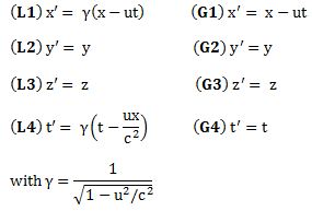
The Galilean or Newtonian rules are the simple rules on the right. Going from one reference frame to another (let’s call them S and S’ respectively) is just a matter of adding or subtracting speeds: if my car goes 100 km/h, and yours goes 120 km/h, then you will see my car falling behind at a speed of (minus) 20 km/h. That’s it. We could also rotate our reference frame, and our Newtonian vector equations would still look the same. As Feynman notes, smilingly, it’s what a lot of armchair philosophers think relativity theory is all about, but so it’s got nothing to do with it. It’s plain wrong!
In any case, back to vectors and transformations. The key to the so-called invariance of the laws of physics is the use of vectors and vector operators that transform like vectors. For example, if we defined A and B as (Ax, Ay, Az) and (Bx, By, Bz), then we knew that the so-called inner product A•B would look the same in all rotated coordinate systems, so we can write: A•B = A’•B’. So we know that if we have a product like that on both sides of an equation, we’re fine: the equation will have the same form in all rotated coordinate systems. Also, the gradient, i.e. our vector operator ∇ = (∂/∂x, ∂/∂y, ∂/∂z), when applied to a scalar function, gave three quantities that also transform like a vector under rotation. We also defined a vector cross product, which yielded a vector (as opposed to the inner product, i.e. the vector dot product, which yields a scalar):

So how does this thing behave under a Galilean transformation? Well… You may or may not remember that we used this cross-product to define the angular momentum L, which was a cross product of the radius vector r and the momentum vector p = mv, as illustrated below. The animation also gives the torque τ, which is, loosely speaking, a measure of the turning force: it’s the cross product of r and F, i.e. the force on the lever-arm.
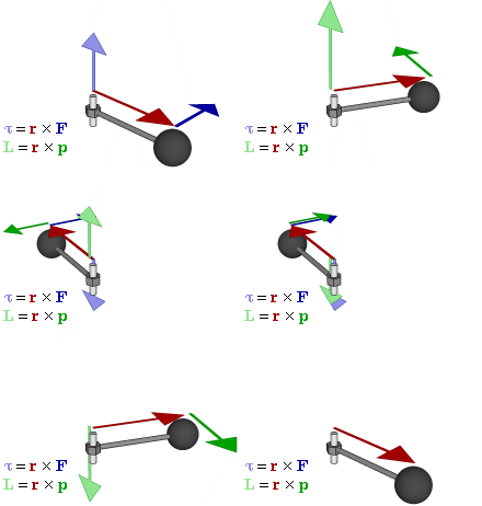
The components of L are:

Now, we find that these three numbers, or objects if you want, transform in exactly the same way as the components of a vector. However, as Feynman points out, that’s a matter of ‘luck’ really. It’s something ‘special’. Indeed, you may or may not remember that we distinguished axial vectors from polar vectors. L is an axial vector, while r and p are polar vectors, and so we find that, in three dimensions, the cross product of two polar vectors will always yields an axial vector. Axial vectors are sometimes referred to as pseudovectors, which suggests that they are ‘not so real’ as… Well… Polar vectors, which are sometimes referred to as ‘true’ vectors. However, it doesn’t matter when doing these Newtonian or Galilean transformations: pseudo or true, both vectors transform like vectors. 🙂
But so… Well… We’re actually getting a bit of a heads-up here: if we’d be mixing (or ‘crossing’) polar and axial vectors, or mixing axial vectors only, so if we’d define something involving L and p (rather than r and p), or something involving L and τ, then we may not be so lucky, and then we’d have to carefully examine our cross-product, or whatever other product we’d want to define, because its components may not behave like a vector.
Huh? Whatever other product we’d want to define? Why are you saying that? Well… We actually can think of other products. For example, if we have two vectors a = (ax, ay, az) and b = (bx, by, bz), then we’ll have nine possible combinations of their components, which we can write as Tij = aibj. So that’s like Lxy, Lyz and Lzx really. Now, you’ll say: “No. It isn’t. We don’t have nine combinations here. Just three numbers.” Well… Think about it: we actually do have nine Lij combinations too here, as we can write: Lij = ri·pj – rj·pi. It just happens that, with this definition, only three of these combinations Lij are independent. That’s because the other six numbers are either zero or the opposite. Indeed, it’s easy to verify that Lij = –Lji , and Lii = 0. So… Well… It turns out that the three components of our L = r×p ‘vector’ are actually a subset of a set of nine Lij numbers. So… Well… Think about it. We cannot just do whatever we want with our ‘vectors’. We need to watch out.
In fact, I do not want to get too much ahead of myself, but I can already tell you that the matrix with these nine Tij = aibj combinations is what is referred to as the tensor. To be precise, it’s referred to as a tensor of the second rank in three dimensions. The ‘second rank’, aka as ‘degree’ or ‘order’ refers to the fact that we’ve got two indices, and the ‘three dimensions’ is because we’re using three-dimensional vectors. We’ll soon see that the electromagnetic tensor is also of the second rank, but it’s a tensor in four dimensions. In any case, I should not get ahead of myself. Just note what I am saying here: the tensor is like a ‘new’ product of two vectors, a new type of ‘cross’ product really (because we’re mixing the components, so to say), but it doesn’t yield a vector: it yields a matrix. For three-dimensional vectors, we get a 3×3 matrix. For four-vectors, we’ll get a 4×4 matrix. And so the full truth about our angular momentum vector L, is the following:
- There is a thing which we call the angular momentum tensor. It’s a 3×3 matrix, so it has nine elements which are defined as: Lij = ri·pj – rj·pi. Because of this definition, it’s an antisymmetric tensor of the second order in three dimensions, so it’s got only three independent components.
- The three independent elements are the components of our ‘vector’ L, and picking them out and calling these three components a ‘vector’ is actually a ‘trick’ that only works in three dimensions. They really just happen to transform like a vector under rotation or under whatever Galilean transformation! [By the way, do you know understand why I was saying that we can look at a tensor as a ‘more general’ cross product?]
- In fact, in four dimensions, we’ll use a similar definition and define 16 elements Fij as Fij = ∇iAj − ∇jAi, using the two four-vectors ∇μ and Aμ (so we have 4×4 = 16 combinations indeed), out of which only six will be independent for the very same reason: we have an antisymmetric vector combination here, Fij = −Fji and Fii = 0. 🙂 However, because we cannot represent six independent things by four things, we do not get some other four-vector, and so that’s why we cannot apply the same ‘trick’ in four dimensions.
However, here I am getting way ahead of myself and so… Well… Yes. Back to the main story line. 🙂 So let’s try to move to the next level of understanding, which is… Well…
Because of guys like Maxwell and Einstein, we now know that rotations are part of the Newtonian world, in which time and space are neatly separated, and that things are not so simple in Einstein’s world, which is the real world, as far as we know, at least! Under a Lorentz transformation, the new ‘primed’ space and time coordinates are a mixture of the ‘unprimed’ ones. Indeed, the new x’ is a mixture of x and t, and the new t’ is a mixture of x and t as well. [Yes, please scroll all the way up and have a look at the transformation on the left-hand side!]
So you don’t have that under a Galilean transformation: in the Newtonian world, space and time are neatly separated, and time is absolute, i.e. it is the same regardless of the reference frame. In Einstein’s world – our world – that’s not the case: time is relative, or local as Hendrik Lorentz termed it quite appropriately, and so it’s space-time – i.e. ‘some kind of union of space and time’ as Minkowski termed it – that transforms.
So that’s why physicists use four-vectors to keep track of things. These four-vectors always have three space-like components, but they also include one so-called time-like component. It’s the only way to ensure that the laws of physics are unchanged when moving with uniform velocity. Indeed, any true law of physics we write down must be arranged so that the invariance of physics (as a “fact of Nature”, as Feynman puts it) is built in, and so that’s why we use Lorentz transformations and four-vectors.
In the mentioned post, I gave a few examples illustrating how the Lorentz rules work. Suppose we’re looking at some spaceship that is moving at half the speed of light (i.e. 0.5c) and that, inside the spaceship, some object is also moving at half the speed of light, as measured in the reference frame of the spaceship, then we get the rather remarkable result that, from our point of view (i.e. our reference frame as observer on the ground), that object is not going as fast as light, as Newton or Galileo – and most present-day armchair philosophers 🙂 – would predict (0.5c + 0.5c = c). We’d see it move at a speed equal to v = 0.8c. Huh? How do we know that? Well… We can derive a velocity formula from the Lorentz rules:

So now you can just put in the numbers now: vx = (0.5c + 0.5c)/(1 + 0.5·0.5) = 0.8c. See?
Let’s do another example. Suppose we’re looking at a light beam inside the spaceship, so something that’s traveling at speed c itself in the spaceship. How does that look to us? The Galilean transformation rules say its speed should be 1.5c, but that can’t be true of course, and the Lorentz rules save us once more: vx = (0.5c + c)/(1 + 0.5·1) = c, so it turns out that the speed of light does not depend on the reference frame: it looks the same – both to the man in the ship as well as to the man on the ground. As Feynman puts it: “This is good, for it is, in fact, what the Einstein theory of relativity was designed to do in the first place—so it had better work!” 🙂
So let’s now apply relativity to electromagnetism. Indeed, that’s what this post is all about! However, before I do so, let me re-write the Lorentz transformation rules for c = 1. We can equate the speed of light to one, indeed, when measure time and distance in equivalent units. It’s just a matter of ditching our seconds for meters (so our time unit becomes the time that light needs to travel a distance of one meter), or ditching our meters for seconds (so our distance unit becomes the distance that light travels in one second). You should be familiar with this procedure. If not, well… Check out my posts on relativity. So here’s the same set of rules for c = 1:
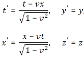
They’re much easier to remember and work with, and so that’s good, because now we need to look at how these rules work with four-vectors and the various operations and operators we’ll be defining on them. Let’s look at that step by step.
Electrodynamics in relativistic notation
Let me copy the Universal Set of Equations and Their Solution once more:
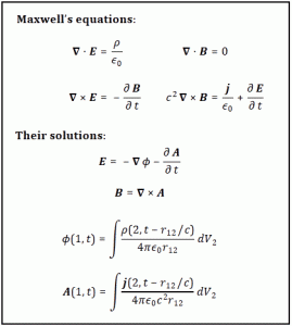
The solution for Maxwell’s equations is given in terms of the (electric) potential Φ and the (magnetic) vector potential A. I explained that in my post on this, so I won’t repeat myself too much here either. The only point you should note is that this solution is the result of a special choice of Φ and A, which we referred to as the Lorentz gauge. We’ll touch upon this condition once more, so just make a mental note of it.
Now, E and B do not correspond to four-vectors: they depend on x, y, z and t, but they have three components only: Ex, Ey, Ez, and Bx, By, and Bz respectively. So we have six independent terms here, rather than four things that, somehow, we could combine into some four-vector. [Does this ring a bell? It should. :-)] Having said that, it turns out that we can combine Φ and A into a four-vector, which we’ll refer to as the four-potential and which we’ll will write as:
Aμ = (Φ, A) = (Φ, Ax, Ay, Az) = (At, Ax, Ay, Az) with At = Φ.
So that’s a four-vector just like R = (ct, x, y, z).
How do we know that Aμ is a four-vector? Well… Here I need to say a few things about those Lorentz transformation rules and, more importantly, about the required condition of invariance under a Lorentz transformation. So, yes, here we need to dive into the math.
Four-vectors and invariance under Lorentz transformations
When you were in high-school, you learned how to rotate your coordinate frame. You also learned that the distance of a point from the origin does not change under a rotation, so you’d write r’2 = x’2 + y’2 + z’2 = r2 = x2 + y2 + z2, and you’d say that r2 is an invariant quantity under a rotation. Indeed, transformations leave certain things unchanged. From the Lorentz transformation rules itself, it is easy to see that
c·t’2 – x’2 – y’2 –z ‘2 = c·t2 –x2 – y2 – z2, or,
if c = 1, that t’2 – x’2 – y’2 – z’2 = t2 – x2 – y2 – z2,
is an invariant under a Lorentz transformation. We found the same for the so-called spacetime interval Δs2 = Δr2 – cΔt2, which we write as Δs2 = Δr2 – Δt2 as we chose our time or distance units such that c = 1. [Note that, from now on, we’ll assume that’s the case, so c = 1 everywhere. We can always change back to our old units when we’re done with the analysis.] Indeed, such invariance allowed us to define spacelike, timelike and lightlike intervals using the so-called light cone emanating from a single event and traveling in all directions.
You should note that, for four-vectors, we do not have a simple sum of three terms. Indeed, we don’t write x2 + y2 + z2 but t2 – x2 – y2 – z2. So we’ve got a +−−− thing here or, it’s just another convention, we could also work with a −+++ sum of terms. The convention is referred to as the signature, and we will use the so-called metric signature here, which is +−−−. Let’s continue the story. Now, all four-vectors aμ = (at, ax, ay, az) have this property that:
at‘2 – ax‘2 – ay‘2 – az‘2 = at2 – ax2 – ay2 – az2.
[The primed quantities are, obviously, the quantities as measured in the other reference frame.] So. Well… Yes. 🙂 But… Well… Hmm… We can say that our four-potential vector is a four-vector, but so we still have to prove that. So we need to prove that Φ’2 – Ax‘2 – Ay‘2 – Az‘2 = Φ2 – Ax2 – Ay2 – Az2 for our four-potential vector Aμ = (Φ, A). So… Yes… How can we do that? The proof is not so easy, but you need to go through it as it will introduce some more concepts and ideas you need to understand.
In my post on the Lorentz gauge, I mentioned that Maxwell’s equations can be re-written in terms of Φ and A, rather than in terms of E and B. The equations are:

The expression look rather formidable, but don’t panic: just look at it. Of course, you need to be familiar with the operators that are being used here, so that’s the Laplacian ∇2 and the divergence operator ∇• that’s being applied to the scalar Φ and the vector A. I can’t re-explain this. I am sorry. Just check my posts on vector analysis. You should also look at the third equation: that’s just the Lorentz gauge condition, which we introduced when deriving these equations from Maxwell’s equations. Having said that, it’s the first and second equation which describe Φ and A as a function of the charges and currents in space, and so that’s what matters here. So let’s unfold the first equation. It says the following:
In fact, if we’d be talking free or empty space, i.e. regions where there are no charges and currents, then the right-hand side would be zero and this equation would then represent a wave equation, so some potential Φ that is changing in time and moving out at the speed c. Here again, I am sorry I can’t write about this here: you’ll need to check one of my posts on wave equations. If you don’t want to do that, you should believe me when I say that, if you see an equation like this:
 then the function Ψ(x, t) must be some function

Now, that’s a function representing a wave traveling at speed c, i.e. the phase velocity. Always? Yes. Always! It’s got to do with the x − ct and/or x + ct argument in the function. But, sorry, I need to move on here.
The unfolding of the equation with Φ makes it clear that we have four equations really. Indeed, the second equation is three equations: one for Ax, one for Ay, and one for Az respectively. The four quantities on the right-hand side of these equations are ρ, jx, jy and jz respectively, divided by ε0, which is a universal constant which does not change when going from one coordinate system to another. Now, the quantities ρ, jx, jy and jz transform like a four-vector. How do we know that? It’s just the charge conservation law. We used it when solving the problem of the fields around a moving wire, when we demonstrated the relativity of the electric and magnetic field. Indeed, the relevant equations were:
You can check that against the Lorentz transformation rules for c = 1. They’re exactly the same, but so we chose t = 0, so the rules are even simpler. Hence, the (ρ, jx, jy, jz) vector is, effectively, a four-vector, and we’ll denote it by jμ = (ρ, j). I now need to explain something else. [And, yes, I know this is becoming a very long story but… Well… That’s how it is.]
It’s about our operators ∇, ∇•, ∇× and ∇2 , so that’s the gradient, the divergence, curl and Laplacian operator respectively: they all have a four-dimensional equivalent. Of course, that won’t surprise you. 😦 Let me just jot all of them down, so we’re done with that, and then I’ll focus on the four-dimensional equivalent of the Laplacian ∇•∇ = ∇2 , which is referred to as the D’Alembertian, and which is denoted by □2, because that’s the one we need to prove that our four-potential vector is a real four-vector. [I know: □2 is a tiny symbol for a pretty monstrous thing, but I can’t help it: my editor tool is pretty limited.]
Now, we’re almost there. Just hang in for a little longer. It should be obvious that we can re-write those two equations with Φ, A, ρ and j, as:

Just to make sure, let me remind you that Aμ = (Φ, A) and that jμ = (ρ, j). Now, our new D’Alembertian operator is just an operator—a pretty formidable operator but, still, it’s an operator, and so it doesn’t change when the coordinate system changes, so the conclusion is that, IF jμ = (ρ, j) is a four-vector – which it is – and, therefore, transforms like a four-vector, THEN the quantities Φ, Ax, Ay, and Az must also transform like a four-vector, which means they are (the components of) a four-vector.
So… Well… Think about it, but not too long, because it’s just an intermediate result we had to prove. So that’s done. But we’re not done here. It’s just the beginning, actually.  Let me repeat our intermediate result:
Aμ = (Φ, A) is a four-vector. We call it the four-potential vector.
OK. Let’s continue. Let me first draw your attention to that expression with the D’Alembertian above. Which expression? This one:
What about it? Well… You should note that the physics of that equation is just the same as Maxwell’s equations. So it’s one equation only, but it’s got it all.
It’s quite a pleasure to re-write it in such elegant form. Why? Think about it: it’s a four-vector equation: we’ve got a four-vector on the left-hand side, and a four-vector on the right-hand side. Therefore, this equation is invariant under a transformation. So, therefore, it directly shows the invariance of electrodynamics under the Lorentz transformation.
Huh? Yes. You may think about this a little longer. 🙂
To wrap this up, I should also note that we can also express the gauge condition using our new four-vector notation. Indeed, we can write it as:
It’s referred to as the Lorentz condition and it is, effectively, a condition for invariance, i.e. it ensures that the four-vector equation above does stay in the form it is in for all reference frames. Note that we’re re-writing it using the four-dimensional equivalent of the divergence operator ∇•, but so we don’t have a dot between ∇μ and Aμ. In fact, the notation is pretty confusing, and it’s easy to think we’re talking some gradient, rather than the divergence. So let me therefore highlight the meaning of both once again. It looks the same, but it’s two very different things: the gradient operates on a scalar, while the divergence operates on a (four-)vector. Also note the +−−− signature is only there for the gradient, not for the divergence!

You’ll wonder why they didn’t use some • or ∗ symbol, and the answer: I don’t know. I know it’s hard to keep inventing symbols for all these different ‘products’ – the ⊗ symbol, for example, is reserved for tensor products, which we won’t get into – but… Well… I think they could have done something here. 😦
In any case… Let’s move on. Before we do, please note that we can also re-write our conservation law for electric charge using our new four-vector notation. Indeed, you’ll remember that we wrote that conservation law as:
Using our new four-vector operator ∇μ, we can re-write that as ∇μjμ = 0. So all of electrodynamics can be summarized in the two equations only—Maxwell’s law and the charge conservation law:
OK. We’re now ready to discuss the electromagnetic tensor. [I know… This is becoming an incredibly long and incredibly complicated piece but, if you get through it, you’ll admit it’s really worth it.]
The electromagnetic tensor
The whole analysis above was done in terms of the Φ and A potentials. It’s time to get back to our field vectors E and B. We know we can easily get them from Φ and A, using the rules we mentioned as solutions:
These two equations should not look as yet another formula. They are essential, and you should be able to jot them down anytime anywhere. They should be on your kitchen door, in your toilet and above your bed. 🙂 For example, the second equation gives us the components of the magnetic field vector B:
Now, look at these equations. The x-component is equal to a couple of terms that involve only y– and z-components. The y-component is equal to something involving only x and z. Finally, the z-component only involves x and y. Interesting. Let’s define a ‘thing’ we’ll denote by Fzy and define as:
So now we can write: Bx = Fzy, By = Fxz, and Bz = Fxy. Now look at our equation for E. It turns out the components of E are equal to things like Fxt, Fyt and Fzt! Indeed, Fxt = ∂Ax/∂t − ∂At/∂x = Ex!
But… Well… No. 😦 The sign is wrong! Ex = −∂Ax/∂t−∂At/∂x, so we need to modify our definition of Fxt. When the t-component is involved, we’ll define our ‘F-things’ as:
So we’ve got a plus instead of a minus. It looks quite arbitrary but, frankly, you’ll have to admit it’s sort of consistent with our +−−− signature for our four-vectors and, in just a minute, you’ll see it’s fully consistent with our definition of the four-dimensional vector operator ∇μ = (∂/∂t, −∂/∂x, −∂/∂y, −∂/∂z). So… Well… Let’s go along with it.
What about the Fxx, Fyy, Fzz and Ftt terms? Well… Fxx = ∂Ax/∂x − ∂Ax/∂x = 0, and it’s easy to see that Fyy and Fzz are zero too. But Ftt? Well… It’s a bit tricky but, applying our definitions carefully, we see that Ftt must be zero too. In any case, the Ftt = 0 will become obvious as we will be arranging these ‘F-things’ in a matrix, which is what we’ll do now. [Again: does this ring a bell? If not, it should. :-)]
Indeed, we’ve got sixteen possible combinations here, which Feynman denotes as Fμν, which is somewhat confusing, because Fμν usually denotes the 4×4 matrix representing all of these combinations. So let me use the subscripts i and j instead, and define Fij as:
Fij = ∇iAj − ∇jAi
with ∇i being the t-, x-, y- or z-component of ∇μ = (∂/∂t, −∂/∂x, −∂/∂y, −∂/∂z) and, likewise, Ai being the t-, x-, y- or z-component of Aμ = (Φ, Ax, Ay, Az). Just check it: Fzy = −∂Ay/∂z + ∂Az/∂y = ∂Az/∂y − ∂Ay/∂z = Bx, for example, and Fxt = −∂Φ/∂x − ∂Ax/∂t = Ex. So the +−−− convention works. [Also note that it’s easier now to see that Ftt = ∂Φ/∂t − ∂Φ/∂t = 0.]
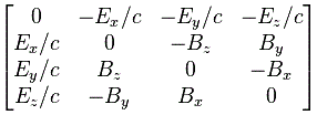
We can now arrange the Fij in a matrix. This matrix is antisymmetric, because Fij = – Fji, and its diagonal elements are zero. [For those of you who love math: note that the diagonal elements of an antisymmetric matrix are always zero because of the Fij = – Fji constraint: just use k = i = j in the constraint.]
Now that matrix is referred to as the electromagnetic tensor and it’s depicted below (we plugged c back in, remember that B’s magnitude is 1/c times E’s magnitude).
So… Well… Great ! We’re done! Well… Not quite. 🙂
We can get this matrix in a number of ways. The least complicated way is, of course, just to calculate all Fij components and them put them in a [Fij] matrix using the i as the row number and the j as the column number. You need to watch out with the conventions though, and so i and j start on t and end on z. 🙂
The other way to do it is to write the ∇μ = (∂/∂t, −∂/∂x, −∂/∂y, −∂/∂z) operator as a 4×1 column vector, which you then multiply with the four-vector Aμ written as a 4×1 row vector. So ∇μAμ is then a 4×4 matrix, which we combine with its transpose, i.e. (∇μAμ)T, as shown below. So what’s written below is (∇μAμ) − (∇μAμ)T.

If you google, you’ll see there’s more than one way to go about it, so I’d recommend you just go through the motions and double-check the whole thing yourself—and please do let me know if you find any mistake! In fact, the Wikipedia article on the electromagnetic tensor denotes the matrix above as Fμν, rather than as Fμν, which is the same tensor but in its so-called covariant form, but so I’ll refer you to that article as I don’t want to make things even more complicated here! As said, there’s different conventions around here, and so you need to double-check what is what really. 🙂
Where are we heading with all of this? The next thing is to look at the Lorentz transformation of these Fij = ∇iAj − ∇jAi components, because then we know how our E and B fields transform. Before we do so, however, we should note the more general results and definitions which we obtained here:
1. The Fμν matrix (a matrix is just a multi-dimensional array, of course) is a so-called tensor. It’s a tensor of the second rank, because it has two indices in it. We think of it as a very special ‘product’ of two vectors, not unlike the vector cross product a × b, whose components were also defined by a similar combination of the components of a and b. Indeed, we wrote:
So one should think of a tensor as “another kind of cross product” or, preferably, and as Feynman puts it, as a “generalization of the cross product”.
2. In this case, the four-vectors are ∇μ = (∂/∂t, −∂/∂x, −∂/∂y, −∂/∂z) and Aμ = (Φ, Ax, Ay, Az). Now, you will probably say that ∇μ is an operator, not a vector, and you are right. However, we know that ∇μ behaves like a vector, and so this is just a special case. The point is: because the tensor is based on four-vectors, the Fμν tensor is referred to as a tensor of the second rank in four dimensions. In addition, because of the Fij = – Fji result, Fμν is an asymmetric tensor of the second rank in four dimensions.
3. Now, the whole point is to examine how tensors transform. We know that the vector dot product, aka the inner product, remains invariant under a Lorentz transformation, both in three as well as in four dimensions, but what about the vector cross product, and what about the tensor? That’s what we’ll be looking at now.
The Lorentz transformation of the electric and magnetic fields
Cross products are complicated, and tensors will be complicated too. Let’s recall our example in three dimensions, i.e. the angular momentum vector L, which was a cross product of the radius vector r and the momentum vector p = mv, as illustrated below (the animation also gives the torque τ, which is, loosely speaking, a measure of the turning force).
The components of L are:
Now, this particular definition ensures that Lij turns out to be an antisymmetric object:

So it’s a similar situation here. We have nine possible combinations, but only three independent numbers. So it’s a bit like our tensor in four dimensions: 16 combinations, but only 6 independent numbers.
Now, it so happens that that these three numbers, or objects if you want, transform in exactly the same way as the components of a vector. However, as Feynman points out, that’s a matter of ‘luck’ really. In fact, Feynman points out that, when we have two vectors a = (ax, ay, az) and b = (bx, by, bz), we’ll have nine products Tij = aibj which will also form a tensor of the second rank (cf. the two indices) but which, in general, will not obey the transformation rules we got for the angular momentum tensor, which happened to be an antisymmetric tensor of the second rank in three dimensions.
To make a long story short, it’s not simple in general, and surely not here: with E and B, we’ve got six independent terms, and so we cannot represent six things by four things, so the transformation rules for E and B will differ from those for a four-vector. So what are they then?
Well… Feynman first works out the rules for the general antisymmetric vector combination Gij = aibj − ajbi, with ai and bj the t-, x-, y- or z-component of the four-vectors aμ = (at, ax, ay, az) and bμ = (bt, bx, by, bz) respectively. The idea is to first get some general rules, and then replace Gij = aibj − ajbi by Fij = ∇iAj − ∇jAi, of course! So let’s apply the Lorentz rules, which – let me remind you – are the following ones:
So we get:
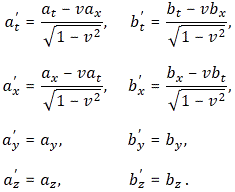
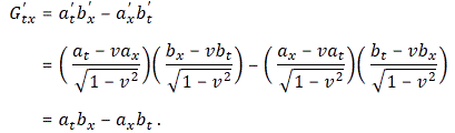
The rest is all very tedious: you just need to plug these things into the various Gij = aibj − ajbi formulas. For example, for G’tx, we get:
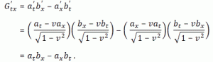
Hey! That’s just G’tx, so we find that G’tx = Gtx! What about the rest? Well… That yields something different. Let me shorten the story by simply copying Feynman here:
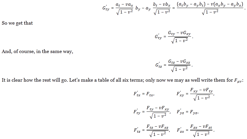
So… Done!
So what?
Well… Now we just substitute. In fact, there are two alternative formulations of the Lorentz transformations of E and B. They are given below (note the units are such that c = 1):
In addition, there is a third equivalent formulation which is more practical, and also simpler, even if it puts the c‘s back in. It re-defines the field components, distinguishing only two:
- The ‘parallel’ components E|| and B|| along the x-direction ( because they are parallel to the relative velocity of the S and S’ reference frames), and
- The ‘perpendicular’ or ‘total transverse’ components E⊥ and B⊥, which are the vector sums of the y- and z-components.
So that gives us four equations only:
And, yes, we are done now. This is the Lorentz transformation of the fields. I am sure it has left you totally exhausted. Well… If not… […] It sure left me totally exhausted. 🙂
To lighten things up, let me insert an image of how the transformed field E actually looks like. The first image is the reference frame of a charge itself: we have a simple Coulomb field. The second image shows the charge flying by. Its electric field is ‘squashed up’. To be precise, it’s just like the scale of x is squashed up by a factor ((1−v2/c2)1/2. Let me refer you to Feynman for the detail of the calculations here.

OK. So that’s it. You may wonder: what about that promise I made? Indeed, when I started this post, I said I’d present a mathematical construct that presents the electromagnetic force as one force only, as one physical reality, but so we’re back writing all of it in terms of two vectors—the electric field vector E and the magnetic field vector B. Well… What can I say? I did present the mathematical construct: it’s the electromagnetic tensor. So it’s that antisymmetric matrix really, which one can combine with a transformation matrix embodying the Lorentz transformation rules. So, I did what I promised to do. But you’re right: I am re-presenting stuff in the old style once again.
The second objection that you may have—in fact, that you should have, is that all of this has been rather tedious. And you’re right. The whole thing just re-emphasizes the value of using the four-potential vector. It’s obviously much easier to take that vector from one reference frame to another – so we just apply the Lorentz transformation rules to Aμ = (Φ, A) and get Aμ‘ = (Φ’, A’) from it – and then calculate E’ and B’ from it, rather than trying to remember those equations above. However, that’s not the point, or…
Well… It is and it isn’t. We wanted to get away from those two vectors E and B, and show that electromagnetism is really one phenomenon only, and so that’s where the concept of the electromagnetic tensor came in. There were two objectives here: the first objective was to introduce you to the concept of tensors, which we’ll need in the future. The second objective was to show you that, while Lorentz’ force law – F = q(E + v×B) makes it clear we’re talking one force only, there is a way of writing it all up that is much more elegant.
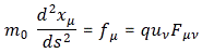
I’ve introduced the concept of tensors here, so the first objective should have been achieved. As for the second objective, I’ll discuss that in my next post, in which I’ll introduce the four-velocity vector μμ as well as the four-force vector fμ. It will explain the following beautiful equation of motion:

Now that looks very elegant and unified, doesn’t it? 🙂
[…] Hmm… No reaction. I know… You’re tired now, and you’re thinking: yet another way of representing the same thing? Well… Yes! So…
OK… Enough for today. Let’s follow up tomorrow.
Some content on this page was disabled on June 16, 2020 as a result of a DMCA takedown notice from The California Institute of Technology. You can learn more about the DMCA here:
https://wordpress.com/support/copyright-and-the-dmca/
Some content on this page was disabled on June 16, 2020 as a result of a DMCA takedown notice from The California Institute of Technology. You can learn more about the DMCA here:
https://wordpress.com/support/copyright-and-the-dmca/
Some content on this page was disabled on June 16, 2020 as a result of a DMCA takedown notice from The California Institute of Technology. You can learn more about the DMCA here:
https://wordpress.com/support/copyright-and-the-dmca/
Some content on this page was disabled on June 16, 2020 as a result of a DMCA takedown notice from The California Institute of Technology. You can learn more about the DMCA here:
https://wordpress.com/support/copyright-and-the-dmca/
Some content on this page was disabled on June 16, 2020 as a result of a DMCA takedown notice from The California Institute of Technology. You can learn more about the DMCA here:
https://wordpress.com/support/copyright-and-the-dmca/
Some content on this page was disabled on June 16, 2020 as a result of a DMCA takedown notice from The California Institute of Technology. You can learn more about the DMCA here:
https://wordpress.com/support/copyright-and-the-dmca/
Some content on this page was disabled on June 16, 2020 as a result of a DMCA takedown notice from The California Institute of Technology. You can learn more about the DMCA here:
https://wordpress.com/support/copyright-and-the-dmca/
Some content on this page was disabled on June 16, 2020 as a result of a DMCA takedown notice from The California Institute of Technology. You can learn more about the DMCA here:
https://wordpress.com/support/copyright-and-the-dmca/
Some content on this page was disabled on June 16, 2020 as a result of a DMCA takedown notice from The California Institute of Technology. You can learn more about the DMCA here:
https://wordpress.com/support/copyright-and-the-dmca/
Some content on this page was disabled on June 16, 2020 as a result of a DMCA takedown notice from The California Institute of Technology. You can learn more about the DMCA here:
https://wordpress.com/support/copyright-and-the-dmca/
Some content on this page was disabled on June 16, 2020 as a result of a DMCA takedown notice from The California Institute of Technology. You can learn more about the DMCA here:
https://wordpress.com/support/copyright-and-the-dmca/
Some content on this page was disabled on June 16, 2020 as a result of a DMCA takedown notice from The California Institute of Technology. You can learn more about the DMCA here:
https://wordpress.com/support/copyright-and-the-dmca/
Some content on this page was disabled on June 16, 2020 as a result of a DMCA takedown notice from The California Institute of Technology. You can learn more about the DMCA here:
https://wordpress.com/support/copyright-and-the-dmca/
Some content on this page was disabled on June 16, 2020 as a result of a DMCA takedown notice from The California Institute of Technology. You can learn more about the DMCA here:
https://wordpress.com/support/copyright-and-the-dmca/
Some content on this page was disabled on June 16, 2020 as a result of a DMCA takedown notice from The California Institute of Technology. You can learn more about the DMCA here:
https://wordpress.com/support/copyright-and-the-dmca/
Some content on this page was disabled on June 16, 2020 as a result of a DMCA takedown notice from The California Institute of Technology. You can learn more about the DMCA here:
https://wordpress.com/support/copyright-and-the-dmca/
Some content on this page was disabled on June 20, 2020 as a result of a DMCA takedown notice from Michael A. Gottlieb, Rudolf Pfeiffer, and The California Institute of Technology. You can learn more about the DMCA here:
https://wordpress.com/support/copyright-and-the-dmca/
Some content on this page was disabled on June 20, 2020 as a result of a DMCA takedown notice from Michael A. Gottlieb, Rudolf Pfeiffer, and The California Institute of Technology. You can learn more about the DMCA here:
https://wordpress.com/support/copyright-and-the-dmca/
Some content on this page was disabled on June 20, 2020 as a result of a DMCA takedown notice from Michael A. Gottlieb, Rudolf Pfeiffer, and The California Institute of Technology. You can learn more about the DMCA here:
https://wordpress.com/support/copyright-and-the-dmca/


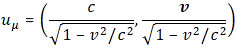 [Note we assume we’re using equivalent time and distance units now, so c = 1 and v/c reduces to a new variable v.]