Understanding gyroscopes

Pre-scriptum (dated 26 June 2020): This post – part of a series of rather simple posts on elementary math and physics – has suffered only a little bit from the attack by the dark force—which is good because I still like it. Only one or two illustrations were removed because of perceived ‘unfair use’, but you will be able to google equivalent stuff. While my views on the true nature of light, matter and the force or forces that act on them have evolved significantly as part of my explorations of a more realist (classical) explanation of quantum mechanics, I think most (if not all) of the analysis in this post remains valid and fun to read. Understanding the dynamics of rotations is extremely important in any realist interpretation of quantum physics. In fact, I would dare to say it is all about rotation!

Original post:

You know a gyroscope: it’s a spinning wheel or disk mounted in a frame that itself is free to alter in direction, so the axis of rotation is not affected as the mounting tilts or moves about. Therefore, gyroscopes are used to provide stability or maintain a reference direction in navigation systems. Understanding a gyroscope itself is simple enough: it only involves a good understanding of the so-called moment of inertia. Indeed, in the previous post, we introduced a lot of concepts related to rotational motion, notably the concepts of torque and angular momentum but, because that post was getting too long, I did not talk about the moment of inertia and gyroscopes. Let me do that now. However, I should warn you: you will not be able to understand this post if you haven’t read or didn’t understand the previous post. So, if you can’t follow, please go back: it’s probably because you didn’t get the other post.

The moment of inertia and angular momentum are related but not quite the same. Let’s first recapitulate angular momentum. Angular momentum is the equivalent of linear momentum for rotational motion:

If we want to change the linear motion of an object, as measured by its momentum p = mv, we’ll need to apply a force. Changing the linear motion means changing either (a) the speed (v), i.e. the magnitude of the velocity vector v, (b) the direction, or (c) both. This is expressed in Newton’s Law, F = m(dv/dt), and so we note that the mass is just a factor of proportionality measuring the inertia to change.
The same goes for angular momentum (denoted by L): if we want to change it, we’ll need to apply a force, or a torque as it’s referred to when talking rotational motion, and such torque can change either (a) L’s magnitude (L), (b) L’s direction or (c) both.

Just like linear momentum, angular momentum is also a product of two factors: the first factor is the angular velocity ω, and the second factor is the moment of inertia. The moment of inertia is denoted by I so we write L = Iω. But what is I? If we’re analyzing a rigid body (which is what we usually do), then it will be calculated as follows:

This is easy enough to understand: the inertia for turning will depend not just on the masses of all of the particles that make up the object, but also on their distance from the axis of rotation–and note that we need to square these distances. The L = Iω formula, combined with the formula for I above, explains why a spinning skater doing a ‘scratch spin’ speeds up tremendously when drawing in his or her arms and legs. Indeed, the total angular momentum has to remain the same, but I becomes much smaller as a result of that r²factor in the formula. Hence, if I becomes smaller, then ω has to go up significantly in order to conserve angular momentum.

Finally, we note that angular momentum and linear momentum can be easily related through the following equation:

That’s all kids stuff. To understand gyroscopes, we’ll have to go beyond that and do some vector analysis. In the previous post, we explained that rotational motion is usually analyzed in terms of torques than forces, and we detailed the relations between force and torque. More in particular, we introduced a torque vector τ with the following components:

τ = (τ_yz, τ_zx, τ_xy) = (τ_x, τ_y, τ_z) with

τ_x = τ_yz = yF_z – zF_y

τ_y = τ_zx = zF_x – xF_z

τ_z = τ_xy = xF_y – yF_x.

We also noted that this torque vector could be written as a cross product of a radius vector and the force: τ = r×F. Finally, we also pointed out the relation between the x-, y- and z-components of the torque vector and the plane of rotation:

(1) τ_x = τ_yz is rotational motion about the x-axis (i.e. motion in the yz-plane)

(2) τ_y = τ_zx is rotational motion about the y-axis (i.e. motion in the zx plane)

(3) τ_z = τ_xy is rotational motion about the z-axis (i.e. motion in the xy-plane)

The angular momentum vector L will have the same direction as the torque vector, but it’s the cross product of the radius vector and the momentum vector: L = r×p. For clarity, I reproduce the animation I used in my previous post once again.

How do we get that cross vector product for L? We noted that τ (i.e. the Greek tau) = dL/dt. So we need to take the time derivative of all three components of L. What are the components of L? They look very similar to those of τ:

L = (L_yz, L_zx, L_xy) = (L_x, L_y, L_z) with

L_x = L_yz = yp_z – zp_y

L_y = L_zx = zp_x – xp_z

L_z = L_xy = xp_y – yp_x.

Now, just check the time derivatives of L_x, L_y, and L_z and you’ll find the components of the torque vector τ. Together with the formulas above, that should be sufficient to convince you that L is, indeed, a vector cross product of r and p: L = r×p.

Again, if you feel this is too difficult, please read or re-read my previous post. But if you do understand everything, then you are ready for a much more difficult analysis, and that’s an explanation of why a spinning top does not fall as it rotates about.

In order to understand that explanation, we’ll first analyze the situation below. It resembles the experiment with the swivel chair that’s often described on ‘easy physics’ websites: the man below holds a spinning wheel with its axis horizontal, and then turns this axis into the vertical. As a result, the man starts to turn himself in the opposite direction.

Let’s now look at the forces and torques involved. These are shown below.

This looks very complicated–you’ll say! You’re right: it is quite complicated–but not impossible to understand. First note the vectors involved in the starting position: we have an angular momentum vector L₀ and an angular velocity vector ω₀. These are both axial vectors, as I explained in my previous post: their direction is perpendicular to the plane of motion, i.e. they are arrows along the axis of rotation. This is in line with what we wrote above: if an object is rotating in the zx-plane (which is the case here), then the angular momentum vector will have a y-component only, and so it will be directed along the y-axis. Which side? That’s determined by the right-hand screw rule. [Again, please do read my previous post for more details if you’d need them.]

So now we have explained L₀ and ω₀. What about all the other vectors? First note that there would be no torque if the man would not try to turn the axis. In that case, the angular momentum would just remain what it is, i.e. dL/dt = 0, and there would be no torque. Indeed, remember that τ = dL/dt, just like F = dp/dt, so dL/dt = 0, then τ = 0. But so the man is turning the axis of rotation and, hence, τ = dL/dt ≠ 0. What’s changing here is not the magnitude of the angular momentum but its direction. As usual, the analysis is in terms of differentials.

As the man turns the spinning wheel, the directional change of the angular momentum is defined by the angle Δθ, and we get a new angular momentum vector L₁. The difference between L₁ and L₀ is given by the vector ΔL. This ΔL vector is a tiny vector in the L₀L₁ plane and, because we’re looking at a differential displacement only, we can say that, for all practical purposes, this ΔL is orthogonal to L₀ (as we move from L₀ to L₁, we’re actually moving along an arc and, hence, ΔL is a tangential vector). Therefore, simple trigonometry allows us to say that its magnitude ΔL will be equal to L₀Δθ. [We should actually write sin(Δθ) but, because we’re talking differentials and measuring angles in radians (so the value reflects arc lengths), we can equate sin(Δθ) with Δθ).]

Now, the torque vector τ has the same direction as the ΔL vector (that’s obvious from their definitions), but what is its magnitude? That’s an easy question to answer: τ = ΔL/Δt = L₀Δθ/Δt = L₀ (Δθ/Δt). Now, this result induces us to define another axial vector which we’ll denote using the same Greek letter omega, but written as a capital letter instead of in lowercase: Ω. The direction of Ω is determined by using that right-hand screw rule which we’ve always been using, and Ω‘s magnitude is equal to Ω = Δθ/Δt. So, in short, Ω is an angular velocity vector just like ω: its magnitude is the speed with which the man is turning the axis of rotation of the spinning wheel, and its direction is determined using the same rules. If we do that, we get the rather remarkable result that we can write the torque vector τ as the cross product of Ω and L₀:

τ = Ω×L₀

Now, this is not an obvious result, so you should check it yourself. When doing that, you’ll note that the two vectors are orthogonal and so we have τ = Ω×L₀ = Ω×L₀ =|Ω||L₀|sin(π/2)n = ΩL₀n with n the normal unit vector given, once again, by the right-hand screw rule. [Note how the order of the two factors in a cross product matters: a×b = –b×a.]

You’re probably tired of this already, and so you’ll say: so what?

Well… We have a torque. A torque is produced by forces, and a torque vector along the z-axis is associated with rotation about the z-axis, i.e. rotation in the xy-plane. Such rotation is caused by the forces F and –F that produce the torque, as shown in the illustration. [Again, their direction is determined by the right-hand screw rule – but I’ll stop repeating that from now on.] But… Wait a minute. First, the direction is wrong, isn’t it? The man turns the other way in reality. And, second, where do these forces come from? Well… The man produces them, and the direction of the forces is not wrong: as the man applies these forces, with his hands, as he holds the spinning wheel and turns it into the vertical direction, equal and opposite forces act on him (cf. the action-reaction principle), and so he starts to turn in the opposite direction.

So there we are: we have explained this complex situation fully in terms of torques and forces now. So that’s good. [If you don’t believe the thing about those forces, just get one of your wheels out of your mountainbike, let it spin, and try to change the plane in which it is spinning: you’ll see you’ll need a bit of force. Not much, but enough, and it’s exactly the kind of force that the man in the illustration is experiencing.]

Now, what if we would not be holding the spinning wheel? What if we would let it pivot, for example? Well… It would just pivot, as shown below.

But… Why doesn’t it fall? Hah! There we are! Now we are finally ready for the analysis we really want to do, i.e. explaining why these spinning tops (or gyros as they’re referred to in physics) don’t fall.

Such spinning top is shown in the illustration below. It’s similar to the spinning wheel: there’s a rotational axis, and we have the force of gravity trying to change the direction of that axis, so it’s like the man turning that spinning wheel indeed, but so now it’s gravity exerting the force that’s needed to change the angular momentum. Let’s associate the vertical direction with the z-axis, and the horizontal place with the xy-axis, and let’s go step-by-step:

The gravitational force wants to pull that spinning top down. So the ΔL vector points downward this time, not upward. Hence, the torque vector will point downward too. But so it’s a torque pointing along the z-axis.
Such torque along the z-axis is associated with a rotation in the xy-plane, so that’s why the spinning top will slowly revolve about the z-axis, parallel to the xy-plane. This process is referred to as precession, and so there’s a precession torque and a precession angular velocity.

So that explains precession and so that’s all there is to it. Now you’ll complain, and rightly so: what I write above, does not explain why the spinning top does not actually fall. I only explained that precession movement. So what’s going on? That spinning top should fall as it precesses, shouldn’t it?

It actually does fall. The point to note, however, is that the precession movement itself changes the direction of the angular momentum vector as well. So we have a new ΔL vector pointing sideways, i.e. a vector in the horizontal plane–so not along the z axis. Hence, we should have a torque in the horizontal plane, and so that implies that we should have two equal and opposite forces acting along the z-axis.

In fact, the right-hand screw rule gives us the direction of those forces: if these forces were effectively applied to the spinning top, it would fall even faster! However, the point to note is that there are no such forces. Indeed, it is not like the man with the spinning wheel: no one (or nothing) is pushing or applying the forces that should produce the torque associated with this change in angular momentum. Hence, because these forces are absent, the spinning top begins to ‘fall’ in the opposite direction of the lacking force, thereby counteracting the gravitational force in such a way that the spinning top just spins about the z-axis without actually falling.

Now, this is, most probably, very difficult to understand in the way you would like to understand it, so just let it sink in and think about it for a while. In this regard, and to help the understanding, it’s probably worth noting that the actual process of reaching equilibrium is somewhat messy. It is illustrated below: if we hold a spinning gyro for a while and then, suddenly, we let it fall (yes, just let it go), it will actually fall. However, as it’s falling, it also starts turning and then, because it starts turning, it also starts ‘falling’ upwards, as explained in that story of the ‘missing force’ above. Initially, the upward movement will overshoot the equilibrium position, thereby slowing the gyro’s speed in the horizontal plane. And so then, because its horizontal speed becomes smaller, it stops ‘falling upward’, and so that means it’s falling down again. But then it starts turning again, and so on and so on. I hope you grasp this–more or less at least. Note that frictional effects will cause the up-and-down movement to dampen out, and so we get a so-called cycloidal motion dampening down to the steady motion we associate with spinning tops and gyros.

That, then, is the ‘miracle’ of a spinning top explained. Is it less of a ‘miracle’ now that we have explained it in terms of torques and missing forces? That’s an appreciation which each of us has to make for him- or herself. I actually find it all even more wonderful now that I can explain it more or less using the kind of math I used above–but then you may have a different opinion.

In any case, let us – to wrap it all up – ask some simple questions about some other spinning objects. What about the Earth for example? It has an axis of rotation too, and it revolves around the Sun. Is there anything like precession going on?

The first answer is: no, not really. The axis of rotation of the Earth changes little with respect to the stars. Indeed, why would it change? Changing it would require a torque, and where would the required force for such torque come from? The Earth is not like a gyro on a pivot being pulled down by some force we cannot see. The Sun attracts the Earth as a whole indeed. It does not change its axis of rotation. That’s why we have a fairly regular day and night cycle.

The more precise answer is: yes, there actually is a very slow axial precession. The whole precessional cycle takes approximately 26,000 years, and it causes the position of stars – as perceived by us, earthlings, that is – to slowly change. Over this cycle, the Earth’s north axial pole moves from where it is now, in a circle with an angular radius of about 23.5 degrees, as illustrated below.

What is this precession caused by? There must be some torque. There is. The Earth is not perfectly spherical: it bulges outward at the equator, and the gravitational tidal forces of the Moon and Sun apply some torque here, attempting to pull the equatorial bulge into the plane of the ecliptic, but instead causing it to precess. So it’s a quite subtle motion, but it’s there, and it’s got also something to do with the gravitational force. However, it’s got nothing to do with the way gravitation makes a spinning top do what it does. [The most amazing thing about this, in my opinion, is that, despite the fact that the precessional movement is so tiny, the Greeks had already discovered it: indeed, the Greek astronomer and mathematician Hipparchus of Nicaea gave a pretty precise figure for this so-called ‘precession of the equinoxes’ in 127 BC.]

What about electrons? Are they like gyros rotating around some pivot? Here the answer is very simple and very straightforward: No, not at all! First, there are no pivots in an atom. Second, the current understanding of an electron – i.e. the quantum-mechanical understanding of a electron – is not compatible with the classical notion of spin. Let me just copy an explanation from Georgia State University’s HyperPhyics website. It basically says it all:

“Experimental evidence like the hydrogen fine structure and the Stern-Gerlach experiment suggest that an electron has an intrinsic angular momentum, independent of its orbital angular momentum. These experiments suggest just two possible states for this angular momentum, and following the pattern of quantized angular momentum, this requires an angular momentum quantum number of 1/2. With this evidence, we say that the electron has spin 1/2. An angular momentum and a magnetic moment could indeed arise from a spinning sphere of charge, but this classical picture cannot fit the size or quantized nature of the electron spin. The property called electron spin must be considered to be a quantum concept without detailed classical analogy.”

So… I guess this should conclude my exposé on rotational motion. I am not sure what I am going to write about next, but I’ll see. 🙂

Post scriptum:

The above treatment is largely based on Feynman’s Lectures.(Vol. I, Chapter 18, 19 and 20). The subject could also be discussed using the concept of a force couple, aka pure moment. A force couple is a system of forces with a resultant moment but no resultant force. Hence, it causes rotation without translation or, more generally, without any acceleration of the centre of mass. In such analysis, we can say that gravity produces a force couple on the spinning top. The two forces of this couple are equal and opposite, and they pull at opposite ends. However, because one end of the top is fixed (friction forces keep the tip fixed to the ground), the force at the other end makes the top go about the vertical axis.

The situation we have is that gravity causes such force couple to appear, just like the man tilting the spinning wheel causes such force couple to appear. Now, the analysis above shows that the direction of the new force is perpendicular to the plane in which the axis of rotation changes, or wants to change in the case of our spinning top. So gravity wants to pull the top down and causes it to move sideways. This horizontal movement will, in turn, create another force couple. The direction of the resultant force, at the free end of the axis of rotation of the top, will, once again, be vertical, but it will oppose the gravity force. So, in a very simplified explanation of things, we could say:

Gravity pulls the top downwards, and causes a force that will make the top move sideways. So the new force, which causes the precession movement, is orthogonal to the gravitation force, i.e. it’s a horizontal force.
That horizontal force will, in turn, cause another force to appear. That force will also be orthogonal to the horizontal force. As we made two 90 degrees turns, so to say, i.e. 180 degrees in total, it means that this third force will be opposite to the gravitational force.
In equilibrium, we have three forces: gravity, the force causing the precession and, finally, a force neutralizing gravity as the spinning top precesses about the vertical axis.

This approach allows for a treatment that is somewhat more intuitive than Feynman’s concept of the ‘missing force.’

Some content on this page was disabled on June 16, 2020 as a result of a DMCA takedown notice from The California Institute of Technology. You can learn more about the DMCA here:

https://wordpress.com/support/copyright-and-the-dmca/
Some content on this page was disabled on June 16, 2020 as a result of a DMCA takedown notice from The California Institute of Technology. You can learn more about the DMCA here:

https://wordpress.com/support/copyright-and-the-dmca/
Some content on this page was disabled on June 16, 2020 as a result of a DMCA takedown notice from The California Institute of Technology. You can learn more about the DMCA here:

https://wordpress.com/support/copyright-and-the-dmca/
Some content on this page was disabled on June 16, 2020 as a result of a DMCA takedown notice from The California Institute of Technology. You can learn more about the DMCA here:

https://wordpress.com/support/copyright-and-the-dmca/

Spinning: the essentials

Pre-scriptum (dated 26 June 2020): These posts on elementary math and physics have not suffered much (if at all) from the attack by the dark force—which is good because I still like them. While my views on the true nature of light, matter and the force or forces that act on them have evolved significantly as part of my explorations of a more realist (classical) explanation of quantum mechanics, I think most (if not all) of the analysis in this post remains valid and fun to read. In fact, I find the simplest stuff is often the best. 🙂

Original post:

When introducing mirror symmetry (P-symmetry) in one of my older posts (time reversal and CPT-symmetry), I also introduced the concept of axial and polar vectors in physics. Axial vectors have to do with rotations, or spinning objects. Because spin – i.e. turning motion – is such an important concept in physics, I’d suggest we re-visit the topic here.

Of course, I should be clear from the outset that the discussion below is entirely classical. Indeed, as Wikipedia puts it: “The intrinsic spin of elementary particles (such as electrons) is quantum-mechanical phenomenon that does not have a counterpart in classical mechanics, despite the term spin being reminiscent of classical phenomena such as a planet spinning on its axis.” Nevertheless, if we don’t understand what spin is in the classical world – i.e. our world for all practical purposes – then we won’t get even near to appreciating what it might be in the quantum-mechanical world. Besides, it’s just plain fun: I am sure you have played, as a kid of as an adult even, with one of those magical spinning tops or toy gyroscopes and so you probably wonder how it really works in physics. So that’s what this post is all about.

The essential concept is the concept of torque. For rotations in space (i.e. rotational motion), the torque is what the force is for linear motion:

It’s the torque (τ) that makes an object spin faster or slower, just like the force would accelerate or decelerate that very same object when it would be moving along some curve (as opposed to spinning around some axis).
There’s also a similar ‘law of Newton’ for torque: you’ll remember that the force equals the time rate-of-change of a vector quantity referred to as (linear) momentum: F = dp/dt = d(mv)/dt = ma (the mass times the acceleration). Likewise, we have a vector quantity that is referred to as angular momentum (L), and we can write: τ (i.e. the Greek tau) = dL/dt.
Finally, instead of linear velocity, we’ll have an angular velocity ω (omega), which is the time rate-of-change of the angle θ defining how far the object has gone around (as opposed to the distance in linear dynamics, describing how far the object has gone along). So we have ω = dθ/dt. This is actually easy to visualize because we know that θ is the length of the corresponding arc on the unit circle. Hence, the equivalence with the linear distance traveled is easily ascertained.

There are numerous other equivalences. For example, we also have an angular acceleration: α = dω/dt = d²θ/dt²; and we should also note that, just like the force, the torque is doing work – in its conventional definition as used in physics – as it turns an object:

ΔW = τ·Δθ

However, we also need to point out the differences. The animation below does that very well, as it relates the ‘new’ concepts – i.e. torque and angular momentum – to the ‘old’ concepts – i.e. force and linear momentum.

So what do we have here? We have vector quantities once again, denoted by symbols in bold-face. However, τ, L and ω are special vectors: axial vectors indeed, as opposed to the polar vectors F, p and v. Axial vectors are directed along the axis of spin – so that is, strangely enough, at right angles to the direction of spin, or perpendicular to the ‘plane of the twist’ as Feynman calls it – and the direction of the axial vector is determined by the direction of spin through one of two conventions: the ‘right-hand screw rule’ or the ‘left-hand screw rule’. Physicists have settled on the former.

If you feel very confused now (I did when I first looked at it), just step back and go through the full argument as I develop it here. It helps to think of torque (also known, for some obscure reason, as the moment of the force) as a twist on an object or a plane indeed: the torque’s magnitude is equal to the tangential component of the force, i.e. F·sin(Δθ), times the distance between the object and the axis of rotation (we’ll denote this distance by r). This quantity is also equal to the product of the magnitude of the force itself and the length of the so-called lever arm, i.e. the perpendicular distance from the axis to the line of action of the force (this lever arm length is denoted by r₀). So we can write τ as:

The product of the tangential component of the force times the distance r: τ = r·F_t = r·F·sin(Δθ)
The product of the length of the lever arm times the force: τ = r₀·F
The torque is the work done per unit of distance traveled: τ = ΔW/Δθ or τ = dW/dθ in the limit.

So… These are actually only the basics, which you should remember from your high-school physics course. If not, have another look at it. We now need to go from scalar quantities to vector quantities to understand that animation above. Torque is not a vector like force or velocity, not a priori at least. However, we can associate torque with a vector of a special type, an axial vector. Feynman calls vectors such as force or (linear) velocity ‘honest’ or ‘real’ vectors. The mathematically correct term for such ‘honest’ or ‘real’ vectors is polar vector. Hence, axial vectors are not ‘honest’ or ‘real’ in some sense: we derive them from the polar vectors. They are, in effect, a so-called cross product of two ‘honest’ vectors. Here we need to explain the difference between a dot and a cross product between two vectors once again:

(1) A dot product, which we denoted by a little dot (·), yields a scalar quantity: a·b = |a||b|cosα = a·b·cosα with α the angle between the two vectors a and b. Note that the dot product of two orthogonal vectors is equal to zero, so take care: τ = r·F_t = r·F·sin(Δθ) is not a dot product of two vectors. It’s a simple product of two scalar quantities: we only use the dot as a mark of separation, which may be quite confusing. In fact, some authors use ∗ for a product of scalars to avoid confusion: that’s not a bad idea, but it’s not a convention as yet. Omitting the dot when multiplying scalars (as I do when I write |a||b|cosα) is also possible, but it makes it a bit difficult to read formulas I find. Also note, once again, how important the difference between bold-face and normal type is in formulas like this: it distinguishes vectors from scalars – and these are two very different things indeed.

(2) A cross product, which we denote by using a cross (×), yields another vector: τ = r×F =|r|·|F|·sinα·n = r·F·sinα·n with n the normal unit vector given by the right-hand rule. Note how a cross product involves a sine, not a cosine – as opposed to a dot product. Hence, if r and F are orthogonal vectors (which is not unlikely), then this sine term will be equal to 1. If the two vectors are not perpendicular to each other, then the sine function will assure that we use the tangential component of the force.

But, again, how do we go from torque as a scalar quantity (τ = r·F_t) to the vector τ = r×F? Well… Let’s suppose, first, that, in our (inertial) frame of reference, we have some object spinning around the z-axis only. In other words, it spins in the xy-plane only. So we have a torque around (or about) the z-axis, i.e. in the xy-plane. The work that will be done by this torque can be written as:

ΔW = F_xΔx + F_yΔy = (xF_y – yF_x)Δθ

Huh? Yes. This results from a simple two-dimensional analysis of what’s going on in the xy-plane: the force has an x- and a y-component, and the distance traveled in the x- and y-direction is Δx = –yΔθ and Δy = xΔθ respectively. I won’t go into the details of this (you can easily find these elsewhere) but just note the minus sign for Δx and the way the x and y get switched in the expressions.

So the torque in the xy-plane is given by τ_xy = ΔW/Δθ = xF_y – yF_x. Likewise, if the object would be spinning about the x-axis – or, what amounts to the same, in the yz-plane – we’d get τ_yz = yF_z – zF_y. Finally, for some object spinning about the y-axis (i.e. in the zx-plane – and please note I write zx, not xz, so as to be consistent as we switch the order of the x, y and z coordinates in the formulas), then we’d get τ_zx = zF_x – xF_z. Now we can appreciate the fact that a torque in some other plane, at some angle with our Cartesian planes, would be some combination of these three torques, so we’d write:

(1) τ_xy = xF_y – yF_x

(2) τ_yz = yF_z – zF_y and

(3) τ_zx = zF_x – xF_z.

Another observer with his Cartesian x’, y’ and z’ axes in some other direction (we’re not talking some observer moving away from us but, quite simply, a reference frame that’s being rotated itself around some axis not necessarily coinciding with any of the x-, y- z- or x’-, y’- and z’-axes mentioned above) would find other values as he calculates these torques, but the formulas would look the same:

(1’) τ_x’y’ = x’F_y’ – y’F_x’

(2’) τ_y’z’ = y’F_z’ – z’F_y’ and

(3’) τ_z’x’ = z’F_x’ – x’F_z’.

Now, of course, there must be some ‘nice’ relationship that expresses the τ_x’y’, τ_y’z’ and τ_z’x’ values in terms of τ_xy, τ_yz, just like there was some ‘nice’ relationship between the x’, y’ and z’ components of a vector in one coordination system (the x’, y’ and z’ coordinate system) and the x, y, z components of that same vector in the x, y and z coordinate system. Now, I won’t go into the details but that ‘nice’ relationship is, in fact, given by transformation expressions involving a rotation matrix. I won’t write that one down here, because it looks pretty formidable, but just google ‘axis-angle representation of a rotation’ and you’ll get all the details you want.

The point to note is that, in both sets of equations above, we have an x-, y- and z-component of some mathematical vector that transform just like a ‘real’ vector. Now, if it behaves like a vector, we’ll just call it a vector, and that’s how, in essence, we define torque, angular momentum (and angular velocity too) as axial vectors. We should note how it works exactly though:

(1) τ_xy and τ_x’y’ will transform like the z-component of a vector (note that we were talking rotational motion about the z-axis when introducing this quantity);

(2) τ_yz and τ_y’z’ will transform like the x-component of a vector (note that we were talking rotational motion about the x-axis when introducing this quantity);

(3) τ_zx and τ_z’x’ will transform like the y-component of a vector (note that we were talking rotation motion when introducing this quantity). So we have

τ = (τ_yz, τ_zx, τ_xy) = (τ_x, τ_y, τ_z) with

τ_x = τ_yz = yF_z – zF_y

τ_y = τ_zx = zF_x – xF_z

τ_z = τ_xy = xF_y – yF_x.

[This may look very difficult to remember but just look at the order: all we do is respect the clockwise order x, y, z, x, y, z, x, etc. when jotting down the x, y and z subscripts.]

Now we are, finally, well equipped to once again look at that vector representation of rotation. I reproduce it once again below so you don’t have to scroll back to that animation:

We have rotation in the zx-plane here (i.e. rotation about the y-axis) driven by an oscillating force F, and so, yes, we can see that the torque vector oscillates along the y-axis only: its x- and z-components are zero. We also have L here, the angular momentum. That’s a vector quantity as well. We can write it as

L = (L_yz, L_zx, L_xy) = (L_x, L_y, L_z) with

L_x = L_yz = yp_z – zp_y (i.e. the angular momentum about the x-axis)

L_y = L_zx = zp_x – xp_z(i.e. the angular momentum about the y-axis)

L_z = L_xy = xp_y – yp_x (i.e. the angular momentum about the z-axis),

And we note, once again, that only the y-component is non-zero in this case, because the rotation is about the y-axis.

We should now remember the rules for a cross product. Above, we wrote that τ = r´F =|r|×|F|×sina×n = = r×F×sina×n with n the normal unit vector given by the right-hand rule. However, a vector product can also be written in terms of its components: c = a´b if and only

c_x = a_yb_z – a_zb_y,

c_y = a_zb_x – a_xb_z, and

c_z = a_xb_y – a_yb_x.

Again, if this looks difficult, remember the trick above: respect the clockwise order when jotting down the x, y and z subscripts. I’ll leave it to you to work out r´F and r´p in terms of components but, when you write it all out, you’ll see it corresponds to the formulas above. In addition, I will also leave it to you to show that the velocity of some particle in a rotating body can be given by a similar vector product: v = ω´r, with ω being defined as another axial vector (aka pseudovector) pointing along the direction of the axis of rotation, i.e. not in the direction of motion. [Is that strange? No. As it’s rotational motion, there is no ‘direction of motion’ really: the object, or any particle in that object, goes round and round and round indeed and, hence, defining some normal vector using the right-hand rule to denote angular velocity makes a lot of sense.]

I could continue to write and write and write, but I need to stop here. Indeed, I actually wanted to tell you how gyroscopes work, but I notice that this introduction has already taken several pages. Hence, I’ll leave the gyroscope for a separate post. So, be warned, you’ll need to read and understand this one before reading my next one.

On (special) relativity: what’s relative?

Pre-scriptum (dated 26 June 2020): These posts on elementary math and physics have not suffered much the attack by the dark force—which is good because I still like them. While my views on the true nature of light, matter and the force or forces that act on them have evolved significantly as part of my explorations of a more realist (classical) explanation of quantum mechanics, I think most (if not all) of the analysis in this post remains valid and fun to read. In fact, I find the simplest stuff is often the best. 🙂

Original post:

This is my third and final post about special relativity. In the previous posts, I introduced the general idea and the Lorentz transformations. I present these Lorentz transformations once again below, next to their Galilean counterparts. [Note that I continue to assume, for simplicity, that the two reference frames move with respect to each other along the x- axis only, so the y- and z-component of u is zero. It is not all that difficult to generalize to three dimensions (especially not when using vectors) but it makes an intuitive understanding of what’s relativity all about more difficult.]

As you can see, under a Lorentz transformation, the new ‘primed’ space and time coordinates are a mixture of the ‘unprimed’ ones. Indeed, the new x’ is a mixture of x and t, and the new t’ is a mixture as well. You don’t have that under a Galilean transformation: in the Newtonian world, space and time are neatly separated, and time is absolute, i.e. it is the same regardless of the reference frame. In Einstein’s world – our world – that’s not the case: time is relative, or local as Hendrik Lorentz termed it, and so it’s space-time – i.e. ‘some kind of union of space and time’ as Minkowski termed it – that transforms. In practice, physicists will use so-called four-vectors, i.e. vectors with four coordinates, to keep track of things. These four-vectors incorporate both the three-dimensional space vector as well as the time dimension. However, we won’t go into the mathematical details of that here.

What else is relative? Everything, except the speed of light. Of course, velocity is relative, just like in the Newtonian world, but the equation to go from a velocity as measured in one reference frame to a velocity as measured in the other, is different: it’s not a matter of just adding or subtracting speeds. In addition, besides time, mass becomes a relative concept as well in Einstein’s world, and that was definitely not the case in the Newtonian world.

What about energy? Well… We mentioned that velocities are relative in the Newtonian world as well, so momentum and kinetic energy were relative in that world as well: what you would measure for those two quantities would depend on your reference frame as well. However, here also, we get a different formula now. In addition, we have this weird equivalence between mass and energy in Einstein’s world, about which I should also say something more.

But let’s tackle these topics one by one. We’ll start with velocities.

Relativistic velocity

In the Newtonian world, it was easy. From the Galilean transformation equations above, it’s easy to see that

v’ = dx’/dt’ = d(x – ut)/dt = dx/dt – d(ut)/dt = v – u

So, in the Newtonian world, it’s just a matter of adding/subtracting speeds indeed: if my car goes 100 km/h (v), and yours goes 120 km/h, then you will see my car falling behind at a speed of (minus) 20 km/h. That’s it. In Einstein’s world, it is not so simply. Let’s take the spaceship example once again. So we have a man on the ground (the inertial or ‘unprimed’ reference frame) and a man in the spaceship (the primed reference frame), which is moving away from us with velocity u.

Now, suppose an object is moving inside the spaceship (along the x-axis as well) with a (uniform) velocity v_x’, as measured from the point of view of the man inside the spaceship. Then the displacement x’ will be equal to x’ = v_x’t’. To know how that looks from the man on the ground, we just need to use the opposite Lorentz transformations: just replace u by –u everywhere (to the man in the spaceship, it’s like the man on the ground moves away with velocity –u), and note that the Lorentz factor does not change because we’re squaring and (–u)²= u². So we get:

Hence, x’ = v_x’t’ can be written as x = γ(v_x’t’ + ut’). Now we should also substitute t’, because we want to measure everything from the point of view of the man on the ground. Now, t = γ(t’ + uv_x’t’/c²). Because we’re talking uniform velocities, v_x(i.e. the velocity of the object as measured by the man on the ground) will be equal to x divided by t (so we don’t need to take the time derivative of x), and then, after some simplifying and re-arranging (note, for instance, how the t’ factor miraculously disappears), we get:

What does this rather complicated formula say? Just put in some numbers:

Suppose the object is moving at half the speed of light, so 0.5c, and that the spaceship is moving itself also at 0.5c, then we get the rather remarkable result that, from the point of view of the observer on the ground, that object is not going as fast as light, but only at v_x = (0.5c + 0.5c)/(1 + 0.5·0.5) = 0.8c.
Or suppose we’re looking at a light beam inside the spaceship, so something that’s traveling at speed c itself in the spaceship. How does that look to the man on the ground? Just put in the numbers: v_x = (0.5c + c)/(1 + 0.5·1) = c ! So the speed of light is not dependent on the reference frame: it looks the same – both to the man in the ship as well as to the man on the ground. As Feynman puts it: “This is good, for it is, in fact, what the Einstein theory of relativity was designed to do in the first place–so it had better work!”

It’s interesting to note that, even if u has no y– or z-component, velocity in the y direction will be affected too. Indeed, if an object is moving upward in the spaceship, then the distance of travel of that object to the man on the ground will appear to be larger. See the triangle below: if that object travels a distance Δs’ = Δy’ = Δy = v’Δt’ with respect to the man in the spaceship, then it will have traveled a distance Δs = vΔt to the man on the ground, and that distance is longer.

I won’t go through the process of substituting and combining the Lorentz equations (you can do that yourself) but the grand result is the following:

v_y = (1/γ)v_y’

1/γ is the reciprocal of the Lorentz factor, and I’ll leave it to you to work out a few numeric examples. When you do that, you’ll find the rather remarkable result that v_y is actually less than v_y’. For example, for u = 0.6c, 1/γ will be equal to 0.8, so v_y will be 20% less than v_y’. How is that possible? The vertical distance is what it is (Δy’ = Δy), and that distance is not affected by the ‘length contraction’ effect (y’ = y). So how can the vertical velocity be smaller? The answer is easy to state, but not so easy to understand: it’s the time dilation effect: time in the spaceship goes slower. Hence, the object will cover the same vertical distance indeed – for both observers – but, from the point of view of the observer on the ground, the object will apparently need more time to cover that distance than the time measured by the man in the spaceship: Δt > Δt’. Hence, the logical conclusion is that the vertical velocity of that object will appear to be less to the observer on the ground.

How much less? The time dilation factor is the Lorentz factor. Hence, Δt = γΔt’. Now, if u = 0.6c, then γ will be equal to 1.25 and Δt = 1.25Δt’. Hence, if that object would need, say, one second to cover that vertical distance, then, from the point of view of the observer on the ground, it would need 1.25 seconds to cover the same distance. Hence, its speed as observed from the ground is indeed only 1/(5/4) = 4/5 = 0.8 of its speed as observed by the man in the spaceship.

Is that hard to understand? Maybe. You have to think through it. One common mistake is that people think that length contraction and/or time dilation are, somehow, related to the fact that we are looking at things from a distance and that light needs time to reach us. Indeed, on the Web, you can find complicated calculations using the angle of view and/or the line of sight (and tons of trigonometric formulas) as, for example, shown in the drawing below. These have nothing to do with relativity theory and you’ll never get the Lorentz transformation out of them. They are plain nonsense: they are rooted in an inability of these youthful authors to go beyond Galilean relativity. Length contraction and/or time dilation are not some kind of visual trick or illusion. If you want to see how one can derive the Lorentz factor geometrically, you should look for a good description of the Michelson-Morley experiment in a good physics handbook such as, yes :-), Feynman’s Lectures.

So, I repeat: illustrations that try to explain length contraction and time dilation in terms of line of sight and/or angle of view are useless and will not help you to understand relativity. On the contrary, they will only confuse you. I will let you think through this and move on to the next topic.

Relativistic mass and relativistic momentum

Einstein actually stated two principles in his (special) relativity theory:

The first is the Principle of Relativity itself, which is basically just the same as Newton’s principle of relativity. So that was nothing new actually: “If a system of coordinates K is chosen such that, in relation to it, physical laws hold good in their simplest form, then the same laws must hold good in relation to any other system of coordinates K’ moving in uniform translation relatively to K.” Hence, Einstein did not change the principle of relativity – quite on the contrary: he re-confirmed it – but he did change Newton’s Laws, as well as the Galilean transformation equations that came with them. He also introduced a new ‘law’, which is stated in the second ‘principle’, and that the more revolutionary one really:
The Principle of Invariant Light Speed: “Light is always propagated in empty space with a definite velocity [speed] c which is independent of the state of motion of the emitting body.”

As mentioned above, the most notable change in Newton’s Laws – the only change, in fact – is Einstein’s relativistic formula for mass:

m_v = γm₀

This formula implies that the inertia of an object, i.e. its mass, also depends on the reference frame of the observer. If the object moves (but velocity is relative as we know: an object will not be moving if we move with it), then its mass increases. This affects its momentum. As you may or may not remember, the momentum of an object is the product of its mass and its velocity. It’s a vector quantity and, hence, momentum has not only a magnitude but also a direction:

p_v = m_vv = γm₀v

As evidenced from the formula above, the momentum formula is a relativistic formula as well, as it’s dependent on the Lorentz factor too. So where do I want to go from here? Well… In this section (relativistic mass and momentum), I just want to show that Einstein’s mass formula is not some separate law or postulate: it just comes with the Lorentz transformation equations (and the above-mentioned consequences in terms of measuring horizontal and vertical velocities).

Indeed, Einstein’s relativistic mass formula can be derived from the momentum conservation principle, which is one of the ‘physical laws’ that Einstein refers to. Look at the elastic collision between two billiard balls below. These balls are equal – same mass and same speed from the point of view of an inertial observer – but not identical: one is red and one is blue. The two diagrams show the collision from two different points of view: left, we have the inertial reference frame, and, right, we have a reference frame that is moving with a velocity equal to the horizontal component of the velocity of the blue ball.

The points to note are the following:

The total momentum of such elastic collision before and after the collision must be the same.
Because the two balls have equal mass (in the inertial reference frame at least), the collision will be perfectly symmetrical. Indeed, we may just turn the diagram ‘upside down’ and change the colors of the balls, as we do below, and the values w, u and v (as well as the angle α) are the same.

As mentioned above, the velocity of the blue and red ball and, hence, their momentum, will depend on the frame of reference. In the diagram on the left, we’re moving with a velocity equal to the horizontal component of the velocity of the blue ball and, therefore, in this particular frame of reference, the velocity (and the momentum) of the blue ball consists of a vertical component only, which we refer to as w.

From this point of view (i.e. the reference frame moving with, the velocity (and, hence, the momentum) of the red ball will have both a horizontal as well as a vertical component. If we denote the horizontal component by u, then it’s easy to show that the vertical velocity of the red ball must be equal to sin(α)v. Now, because u = cos(α)v, this vertical component will be equal to tan(α)u. But so what is tan(α)u? Now, you’ll say, that is quite evident: tan(α)u must be equal to w, right?

No. That’s Newtonian physics. The red ball is moving horizontally with speed u with respect to the blue ball and, hence, its vertical velocity will not be quite equal to w. Its vertical velocity will be given by the formula which we derived above: v_y = (1/γ)v_y’, so it will be a little bit slower than the w we see in the diagram on the right which is, of course, the same w as in the diagram on the left. [If you look carefully at my drawing above, then you’ll notice that the w vector is a bit longer indeed.]

Huh? Yes. Just think about it: tan(α)u = (1/γ)w. But then… How can momentum be conserved if these speeds are not the same? Isn’t the momentum conservation principle supposed to conserve both horizontal as well as vertical momentum? It is, and momentum is being conserved. Why? Because of the relativistic mass factor.

Indeed, the change in vertical momentum (Δp) of the blue ball in the diagram on the left or – which amounts to the same – the red ball in the diagram on the right (i.e. the vertically moving ball) is equal to Δp_blue = 2m_ww. [The factor 2 is there because the ball goes down and then up (or vice versa) and, hence, the total change in momentum must be twice the m_ww amount.] Now, that amount must be equal to Δp_red, which is equal to Δp_blue = 2m_v(1/γ)w. Equating both yields the following grand result:

m_v/m_w= γ ⇔ m_v= γm_w

What does this mean? It means that mass of the red ball in the diagram on the left is larger than the mass of the blue ball. So here we have actually derived Einstein’s relativistic mass formula from the momentum conservation principle !

Of course you’ll say: not quite. This formula is not the m_u= γm₀formula that we’re used to ! Indeed, it’s not. The blue ball has some velocity w itself, and so the formula links two velocities v and w. However, we can derive m_v= γm₀formula as a limit of m_v= γm_w for w going to zer0. How can w become infinitesimally small? If the angle α becomes infinitesimally small. It’s obvious, then, that v and u will be practically equal. In fact, if w goes to zero, then m_wwill be equal to m₀in the limiting case, and m_vwill be equal to m_u. So, then, indeed, we get the familiar formula as a limiting case:

m_u= γm₀

Hmm… You’ll probably find all of this quite fishy. I’d suggest you just think about it. What I presented above, is actually Feynman’s presentation of the subject, but with a bit more verbosity. Let’s move on to the final.

Relativistic energy

From what I wrote above (and from what I wrote in my two previous posts on this topic), it should be obvious, by now, that energy also depends on the reference frame. Indeed, mass and velocity depend on the reference frame (moving or not), and both appear in the formula for kinetic energy which, as you’ll remember, is

K.E. = mc²– m₀c²= (m – m₀)c²= γm₀c²– m₀c²= m₀c²(γ – 1).

Now, if you go back to the post where I presented that formula, you’ll see that we’re actually talking the change in kinetic energy here: if the mass is at rest, it’s kinetic energy is zero (because m = m₀), and it’s only when the mass is moving, that we can observe the increase in mass. [If you wonder how, think about the example of the fast-moving electrons in an electron beam: we see it as an increase in the inertia: applying the same force does no longer yield the same acceleration.]

Now, in that same post, I also noted that Einstein added an equivalent rest mass energy (E₀= m₀c²) to the kinetic energy above, to arrive at the total energy of an object:

E = E₀+ K.E. = mc²

Now, what does this equivalence actually mean? Is mass energy? Can we equate them really? The short answer to that is: yes.

Indeed, in one of my older posts (Loose Ends), I explained that protons and neutrons are made of quarks and, hence, that quarks are the actual matter particles, not protons and neutrons. However, the mass of a proton – which consists of two up quarks and one down quark – is 938 MeV/c²(don’t worry about the units I am using here: because protons are so tiny, we don’t measure their mass in grams), but the mass figure you get when you add the rest mass of two u‘s and one d, is 9.6 MeV/c²only: about one percent of 938 ! So where’s the difference?

The difference is the equivalent mass (or inertia) of the binding energy between the quarks. Indeed, the so-called ‘mass’ that gets converted into energy when a nuclear bomb explodes is not the mass of quarks. Quarks survive: nuclear power is binding energy between quarks that gets converted into heat and radiation and kinetic energy and whatever else a nuclear explosion unleashes.

In short, 99% of the ‘mass’ of a proton or an electron is due to the strong force. So that’s ‘potential’ energy that gets unleashed in a nuclear chain reaction. In other words, the rest mass of the proton is actually the inertia of the system of moving quarks and gluons that make up the particle. In such atomic system, even the energy of massless particles (e.g. the virtual photons that are being exchanged between the nucleus and its electron shells) is measured as part of the rest mass of the system. So, yes, mass is energy. As Feynman put it, long before the quark model was confirmed and generally accepted:

“We do not have to know what things are made of inside; we cannot and need not justify, inside a particle, which of the energy is rest energy of the parts into which it is going to disintegrate. It is not convenient and often not possible to separate the total mc²energy of an object into (1) rest energy of the inside pieces, (2) kinetic energy of the pieces, and (3) potential energy of the pieces; instead we simply speak of the total energy of the particle. We ‘shift the origin’ of energy by adding a constant m₀c²to everything, and say that the total energy of a particle is the mass in motion times c², and when the object is standing still, the energy is the mass at rest times c².” (Richard Feynman’s Lectures on Physics, Vol. I, p. 16-9)

So that says it all, I guess, and, hence, that concludes my little ‘series’ on (special) relativity. I hope you enjoyed it.

Post scriptum:

Feynman describes the concept of space-time with a nice analogy: “When we move to a new position, our brain immediately recalculates the true width and depth of an object from the ‘apparent’ width and depth. But our brain does not immediately recalculate coordinates and time when we move at high speed, because we have had no effective experience of going nearly as fast as light to appreciate the fact that time and space are also of the same nature. It is as though we were always stuck in the position of having to look at just the width of something, not being able to move our heads appreciably one way or the other; if we could, we understand now, we would see some of the other man’s time—we would see “behind”, so to speak, a little bit. Thus, we shall try to think of objects in a new kind of world, of space and time mixed together, in the same sense that the objects in our ordinary space-world are real, and can be looked at from different directions. We shall then consider that objects occupying space and lasting for a certain length of time occupy a kind of a “blob” in a new kind of world, and that when we look at this “blob” from different points of view when we are moving at different velocities. This new world, this geometrical entity in which the “blobs” exist by occupying position and taking up a certain amount of time, is called space-time.”

If none of what I wrote could convey the general idea, then I hope the above quote will. 🙂 Apart from that, I should also note that physicists will prefer to re-write the Lorentz transformation equations by measuring time and distance in so-called equivalent units: velocities will be expressed not in km/h but as a ratio of c and, hence, c = 1 (a pure number) and so u will also be a pure number between 0 and 1. That can be done by expressing distance in light-seconds ( a light-second is the distance traveled by light in one second or, alternatively, by expressing time in ‘meter’. Both are equivalent but, in most textbooks, it will be time that will be measured in the ‘new’ units. So how do we express time in meter?

It’s quite simple: we multiply the old seconds with c and then we get: time_{expressed in meters}= time_{expressed in seconds}multiplied by 3×10⁸meters per second. Hence, as the ‘second’ the first factor and the ‘per second’ in the second factor cancel out, the dimension of the new time unit will effectively be the meter. Now, if both time and distance are expressed in meter, then velocity becomes a pure number without any dimension, because we are dividing distance expressed in meter by time expressed in meter, and it should be noted that it will be a pure number between 0 and 1 (0 ≤ u ≤ 1), because 1 ‘time second’ = 1/(3×10⁸) ‘time meters’. Also, c itself becomes the pure number 1. The Lorentz transformation equations then become:

They are easy to remember in this form (cf. the symmetry between x – ut and t – ux) and, if needed, we can always convert back to the old units to recover the original formulas.

I personally think there is no better way to illustrate how space and time are ‘mere shadows’ of the same thing indeed: if we express both time and space in the same dimension (meter), we can see how, as result of that, velocity becomes a dimensionless number between zero and one and, more importantly, how the equations for x’ and t’ then mirror each other nicely. I am not sure what ‘kind of union’ between space and time Minkowski had in mind, but this must come pretty close, no?

Final note: I noted the equivalence of mass and energy above. In fact, mass and energy can also be expressed in the same units, and we actually do that above already. If we say that an electron has a rest mass of 0.511 MeV/c²(a bit less than a quarter of the mass of the u quark), then we express the mass in terms of energy. Indeed, the eV is an energy unit and so we’re actually using the m = E/c² formula when we express mass in such units. Expressing mass and energy in equivalent units allows us to derive similar ‘Lorentz transformation equations’ for the energy and the momentum of an object as measured under an inertial versus a moving reference frame. Hence, energy and momentum also transform like our space-time four-vectors and – likewise – the energy and the momentum itself, i.e. the components of the (four-)vector, are less ‘real’ than the vector itself. However, I think this post has become way too long and, hence, I’ll just jot these four equations down – please note, once again, the nice symmetry between (1) and (2) – but then leave it at that and finish this post. 🙂

On (special) relativity: the Lorentz transformations

Original post:

I just skyped to my kids (unfortunately, we’re separated by circumstances) and they did not quite get the two previous posts (on energy and (special) relativity). The main obstacle is that they don’t know much – nothing at all actually – about integrals. So I should avoid integrals. That’s hard but I’ll try to do so in this post, in which I want to introduce special relativity as it’s usually done, and so that’s not by talking about Einstein’s mass-energy equivalence relation first.

Galilean/Newtonian relativity

A lot of people think they understand relativity theory but they often confuse it with Galilean (aka Newtonian) relativity and, hence, they actually do not understand it at all. Indeed, Galilean or Newtonian relativity is as old as Galileo and Newton (so that’s like 400 years old), who stated the principle of relativity as a corollary to the laws of motion: “The motions of bodies included in a given space are the same amongst themselves, whether that space is at rest or moves uniformly forward in a straight line.”

The Galilean or Newtonian principle of relativity is about adding and subtracting speeds: if I am driving at 120 km/h on some highway, but you overtake me at 140 km/h, then I will see you go past me at the rather modest speed of 20 km/h. That’s all what there is to it.

Now, that’s not what Einstein‘s relativity theory is about. Indeed, the relationship between your and my reference frame (yours is moving with respect to mine, and mine is moving with respect to yours but with opposite velocity) is very simple in this example. It involves a so-called Galilean transformation only: if my coordinate system is (x, y, z, t), and yours is (x‘, y‘, z‘, t‘), then we can write:

(1) x’ = x – ut (or x = x’ + ut), (2) y’ = y, (3) z’ = z and (4) t’ = t

To continue the example above: if we start counting at t = t’ = 0 when you are overtaking me, and if we both consider ourselves to be at the center of our reference frame (i.e. x = 0 where I am and x’ = 0 where you are), then you will be at x = 10 km after 30 minutes from my point of view, and I will be at x’ = –10 km (so that’s 10 km behind) from your point of view. So x’ = x – ut indeed, with u = 20 km/h.

Again, that’s not what Einstein’s principle of relativity is about. They knew that very well in the 17th century already. In fact, they actually knew that much earlier but Descartes formalized his Cartesian coordinate system only in the first half of the 17th century and, hence, it’s only from that time onwards that scientists such as Newton and Huygens started using it to transform the laws of physics from one frame of reference to another. What they found is that those laws remained invariant.

For example, the conservation law for momentum remains valid even if, as illustrated below, an inertial observer will see an elastic collision, such as the one illustrated, differently than a observer who’s moving along: for the observer who’s moving along, the (horizontal) speed of the blue ball will be zero, and the (horizontal) speed of the red ball will be twice the speed as observed by the inertial observer. That being said, both observers will find that momentum (i.e. the product of mass and velocity: p = mv) is being conserved in such collisions.

But, again, that’s Galilean relativity only: the laws of Newton are of the same form in a moving system as in a stationary system and, therefore, it is impossible to tell, by making experiments, whether our system is moving or not. In other words: there is no such thing as ‘absolute speed’. But, so – let me repeat it again – that is not what Einstein’s relativity theory is about.

Let me give a more interesting example of Galilean relativity, and then we can see what’s wrong with it. The speed of a sound wave is not dependent on the motion of the source: the sound of a siren of an ambulance or a noisy car engine will always travel at a speed of 343 meter per second, regardless of the motion of the ambulance. So, while we’ll experience a so-called Doppler effect when the ambulance is moving – i.e. a higher pitch when it’s approaching than when it’s receding – this Doppler effect does not have any impact on the speed of the sound wave. It only affects the frequency as we hear it. The speed of the wave depends on the medium only, i.e. air in this case.

Indeed, the speed of sound will be different in another gas, or in a fluid, or in a solid, and there’s a surprisingly simple function for that – the so-called Newton-Laplace equation: v_sound = (k/ρ)². In this equation, k is a coefficient of ‘stiffness’ of the medium (even if ‘stiffness’ sounds somewhat strange as a concept to apply to gases), and ρ is the density of the medium (so lower or higher air density will increase/decrease the speed of sound).

This has nothing to do with speed being absolute. No. The Galilean relativity principle does come into play, as one would expect: it is actually possible to catch up with a sound wave (or with any wave traveling through some medium). In fact, that’s what supersonic planes do: they catch up with their own sound waves. However, in essence, planes are not any different from cars in terms of their relationship with the sound that they produce. It’s just that they are faster: the sound wave they produce also travels at a speed of 1,235 km/h, and so cars can’t match that, but supersonic planes can!

[As for the shock wave that is being produced as these planes accelerate and actually ‘break’ the ‘sound barrier’, that has to do with the pressure waves the plane creates in front of itself (just like a traveling compresses the air in front of it). These pressure waves also travel at the speed of sound. Now, as the speed of the object increases, the waves are forced together, or compressed, because they cannot get out of the way of each other. Eventually they merge into one single shock wave, and so that’s what happens and creates the ‘sonic boom’, which also travels at the speed of sound. However, that should not concern us here. For more information on this, I’d refer to Wikipedia, as I got these illustrations from that source, and I quite like the way they present the topic.]

The Doppler effect looks somewhat different (it’s illustrated above) but so, once again, this phenomenon has nothing to do with Einstein’s relativity theory. Why not? Because we are still talking Galilean relativity here. Indeed, let’s suppose our plane travels at twice the speed of sound (i.e. Mach 2 or almost 2,500 km/h). For us, as inertial observers, the speed of the sound wave originating at point 0 in the illustration above (i.e. the reference frame of the inertial observer) will be equal to dx/dt = 1235 km/h. However, for the pilot, the speed of that wave will be equal to

dx’/dt = d(x – ut)/dt = dx/dt – d(ut)/dt = dx/dt – d(ut)/dt = 1235 km/h – u

= 1235 km/h – u = 1235 km/h – 2470 km/h = – 1235 km/h

In short, from the point of view of the pilot, he sees the wave front of the wave created at point 0 traveling away from him (cf. the negative value) at 1235 km/h, i.e. the speed of sound. That makes sense obviously, because he travels twice as fast. However – I cannot repeat it enough – this phenomenon has nothing to do with Einstein’s theory of relativity: if they could have imagined supersonic travel, Galileo, Newton and Huygens would have predicted that too.

So what’s Einstein’s theory of (special) relativity about?

Einstein’s principle of relativity

In 1865, the Scottish mathematical physicist James Clerk Maxwell – I guess it’s important to note he’s Scottish with that referendum coming 🙂 – finally discovered that light was nothing but electromagnetic radiation – so radio waves, (visible) light, X-rays, gamma rays,… It’s all the same: electromagnetic radiation, also known as light tout court.

Now, the equations that describe how electromagnetic radiation (i.e. light) travels through space are beautiful but involve operators which you may not recognize and, hence, I will not write them down. The point to note is that Maxwell’s equations were very elegant but… There were two major difficulties with them:

They did not respect Galilean relativity: if we transform them using the above-mentioned Galilean transformation (x’ = x – ut, y’ = y, z’ = z and t’ = t) then we do not get some relative speed of light. On the contrary, according to Maxwell’s equations, from whatever reference frame you look at light, it should always travel at the same (absolute) speed of light c = 299,792 km/h. So c is a constant, and the same constant, ALWAYS.
Scientists did not have any clue about the medium in which light was supposed to travel. The second half of the 19th century saw lots of experiments trying to discover evidence of a hypothetical ‘luminiferous aether’ in which light was supposed to travel, and which should also have some ‘stiffness’ and ‘density’, but so they could not find any trace of it. No one ever did, and so now we’ve finally accepted that light can actually travel in a vacuum, i.e. in plain nothing.

So what? Well… Let’s first look at the first point. Just like a sound wave, the motion of the source does not have any impact on the speed of light: it goes out in all directions at the same speed c, whether it is emitted from a fast-moving car or from some beacon near the sea. However, unlike sound waves, Maxwell’s equations imply that we cannot catch up with them. That’s troublesome, very troublesome, because, according to the above-mentioned Galilean transformation rules,

i.e. v’ = dx’/dt = dx/dt – u = v – u,

some light beam that is traveling at speed v = c past a spaceship that itself is traveling at speed u – let’s say u = 0.2c for example – should have a speed of c‘ = c – 0.2c = 0.8c = = 239,834 km/h only with respect to the spaceship. However, that’s not what Maxwell’s equations say when you substitute x, y, z and t for x‘, y‘, z‘ and t‘ using those four simple equations x’ = x – ut, y’ = y, z’ = z and t’ = t. After you do the substitution, the transformed Maxwell equations will once again yield that c’ = c = 299,792 km/h, and not c’ = 0.8×299,792 km/h = 239,834 km/h.

That’s weird ! Why? Well… If you don’t think that this is weird, then you’re actually not thinking at all ! Just compare it with the example of our sound wave. There is just no logic to it !

The discovery startled all scientists because there could only be possible solutions to the paradox:

Either Maxwell’s equations were wrong (because they did not observe the principle of (Galilean relativity) or, else,
Newton’s equations (and the Galilean transformation rules – i.e. the Galilean relativity principle) are wrong.

Obviously, scientists and experimenters first tried to prove that Maxwell had it all wrong – if only because no experiment had ever shown Newton’s Laws to be wrong, and so it was probably hard – if not impossible – to try to come up with one that would ! So, instead, experimenters invented all kinds of wonderful apparatuses trying to show that the speed of the light was actually not absolute.

Basically, these experiments assumed that the speed of the Earth, as it rotates around the Sun at a speed of 108,000 km per hour, would result in measurable differences of c that would depend on the direction of the apparatus. More specifically, the speed of the light beam, as measured, would be different if the light beam would be traveling parallel to the motion of the Earth, as opposed to the light beam traveling at right angle to the motion of the Earth. Why? Well… It’s the same idea as the car chasing its own light beams, but I’ll refer to you to other descriptions of the experiment, because explaining these set-ups would take too much time and space. 🙂 I’ll just say that, because 108,000 km/h (on average) is only about 30 km per second (i.e. 0.0001 times c), these experiments relied on (expected) interference effects. The technical aspect of these experiments is really quite interesting. However, as mentioned above, I’ll refer you to Wikipedia or other sources if you’d want more detail.

Just note the most famous of those experiments: the 1887 Michelson-Morley experiment, also known as ‘the most famous failed experiment in history’ because, indeed, it failed to find any interference effects: the speed of light always was the speed of light, regardless of the direction of the beam with respect to the direction of motion of the Earth.

The Lorentz transformations

Once the scientists had recovered from this startling news (Michelson himself suffered from a nervous breakdown for a while, because he really wanted to find that interference effect in order to disprove Maxwell’s Laws), they suggested solutions.

The math was solved first. Indeed, just before the turn of the century, the Dutch physicist Hendrik Antoon Lorentz suggested that, if material bodies would contract in the direction of their motion with a factor (1 – u²/c²)^1/2 and, in addition, if time would also be dilated with a factor (1 – u²/c²)^–1/2, then the Michelson-Morley results could be explained. Of course, scientists objected to this ‘explanation’ as being very much ‘ad hoc’.

So then came Einstein. He just took the math for granted, so Einstein basically accepted the so-called Lorentz transformations that resulted from it, and corrected Newton’s Law in order to set physics right again.

And so that was it. As it turned out, all that was needed in fact, was to do away with the assumption that the inertia (or mass) of an object is a constant and, hence, that it does not vary with its velocity. For us, today, it seems obvious: mass also varies, and the factor involved is the very same Lorentz factor that we mentioned above: γ = (1 – u²/c²)^–1/2. Hence, the m in Newton’s Second Law (F = d(mv)/dt) is not a constant but equal to m = γm₀. For all speeds that we, human beings, can imagine (including the astronomical speed of the Earth in orbit around the Sun), the ‘correction’ is too small to be noticeable, or negligible, but so it’s there, as evidenced by the Michelson-Morley experiment, and, some hundred years later, we can actually verify it in particle accelerators.

As said, for us, today, it’s obvious (in my previous post, I mention a few examples: I explain how the mass of electrons in an electron beam is impacted by their speed, and how the lifetime of muon increases because of their speed) but one hundred years ago, it was not. Not at all – and so that’s why Einstein was a genius: he dared to explore and accept the non-obvious.

Now, what then are the correct transformations from one reference frame to another? They are referred to as the Lorentz transformations, and they can be written down (in a simplified form, assuming relative motion in the x direction only) as follows:

Now, I could point out many interesting implications, or come up with examples, but I will resist the temptation. I will only note two things about them:

1. These Lorentz transformations actually re-establish the principle of relativity: the Laws of Nature – including the Laws of Newton as corrected by Einstein’s relativistic mass formula – are of the same form in a moving system as in a stationary system, and therefore it is impossible to tell, by making experiments, whether the system is moving or not.

2. The second thing I should note is that the equations above imply that the idea of absolute time is no longer valid: there is no such thing as ‘absolute’ or ‘universal’ time. Indeed, Lorentz’ concept of ‘local time’ is a most profound departure from Newtonian mechanics that is implicit in these equations.

Indeed, space and time are entangled in these equations as you can see from the –ut and –ux/c² terms in the equation for x’ and t’ respectively and, hence, the idea of simultaneity has to be abandoned: what happens simultaneously in two separated places according to one observer, does not happen at the same time as viewed by an observer moving with respect to the first. Let me quickly show how.

Suppose that in my world I see two events happening at the same time t₀but so they happen at two different places x₁ and x₂. Now, if you are movingaway from me at a (uniform) speed u, then equation (4) tells us that you will see these two events happen at two different times t₁‘ and t₂‘, with the time difference t₁‘ – t₂‘ equal to t₁‘ – t₂‘ = γ[u(x₁ – x₂)/c²], with γ the above-mentioned Lorentz factor. [Just do the calculation for yourself using equation 4.]

Of course, the effect is negligible for most speeds that we, as human beings, can imagine, but it’s there. So we do not have three separate space coordinates and one time coordinates, but four space-time coordinates that transform together, fully entangled, when applying those four equations above.

That observation led the German mathematician Hermann Minkowski, who helped Einstein to develop his theory of four-dimensional space-time, to famously state that “Space of itself, and time of itself, will sink into mere shadows, and only a kind of union between them shall survive.”

Post scriptum: I did not elaborate on the second difficulty when I mentioned Maxwell’s equations: the lack of a need for a medium for light to travel through. I will let that rest for the moment (or, else, you can just Google some stuff on it). Just note that (1) it is kinda convenient that electromagnetic radiation does not need any medium (I can’t see how one would incorporate that in relativity theory) and (2) that light does seem to slow down in a medium. However, the explanation for that (i.e. for light to have an apparently lower speed in a medium) is to be found in quantum mechanics and so we won’t touch upon that complex matter here (for now that is). The point to note is that this slowing down is caused by light interacting with the matter it encounters as it travels through the medium. It does not actually go slower. However, I need to stop here as this is, yet again, a post which has become way too long. On the other hand, I am hopeful my kids will actually understand this one, because it does not involve integrals. 🙂

Another post for my kids: introducing (special) relativity

Original post:

In my previous post, I talked about energy, and I tried to keep it simple – but also accurate. However, to be completely accurate, one must, of course, introduce relativity at some point. So how does that work? What’s ‘relativistic’ energy? Well… Let me try to convey a few ideas here.

The first thing to note is that the energy conservation law still holds: special theory or not, the sum of the kinetic and potential energies in a (closed) system is always equal to some constant C. What constant? That doesn’t matter: Nature does not care about our zero point and, hence, we can add or subtract any (other) constant to the equation K.E. + P.E. = T + U = C.

That being said, in my previous post, I pointed out that the constant depends on the reference point for the potential energy term U: we will usually take infinity as the reference point (for a force that attracts) and associate it with zero potential (U = 0). We then get a function U(x) like the one below: for gravitational energy we have U(x) = –GMm/x, and for electrical charges, we have U(x) = q₁q₂/4πε₀x. The mathematical shape is exactly the same but, in the case of the electromagnetic forces, you have to remember that likes repel, and opposites attract, so we don’t need the minus sign: the sign of the charges takes care of it.

Minus sign? In case you wonder why we need that minus sign for the potential energy function, well… I explained that in my previous post and so I’ll be brief on that here: potential energy is measured by doing work against the force. That’s why. So we have an infinite sum (i.e. an integral) over some trajectory or path looking like this: U = – ∫F·ds.

For kinetic energy, we don’t need any minus sign: as an object picks up speed, it’s the force itself that is doing the work as its potential energy is converted into kinetic energy, so the change in kinetic energy will equal the change in potential energy, but with opposite sign: as the object loses potential energy, it gains kinetic energy. Hence, we write ΔT = –ΔU = ∫F·ds..

That’s all kids stuff obviously. Let’s go beyond this and ask some questions. First, why can we add or subtract any constant to the potential energy but not to the kinetic energy? The answer is… Well… We actually can add or subtract a ‘constant’ to the kinetic energy as well. Now you will shake your head: Huh? Didn’t we have that T = mv²/2 formula for kinetic energy? So how and why could one add or subtract some number to that?

Well… That’s where relativity comes into play. The velocity v depends on your reference frame. If another observer would move with and/or alongside the object, at the same speed, that observer would observe a velocity equal to zero and, hence, its kinetic energy – as that observer would measure it – would also be zero. You will object to that, saying that a change of reference frame does not change the force, and you’re right: the force will cause the object to accelerate or decelerate indeed, and if the observer is not subject to the same force, then he’ll see the object accelerate or decelerate indeed, regardless of his reference frame is a moving or inertial frame. Hence, both the inertial as well as the moving observer will see an increase (or decrease) in its kinetic energy and, therefore, both will conclude that its potential energy decreases (or increases) accordingly. In short, it’s the change in energy that matters, both for the potential as well as for the kinetic energy. The reference point itself, i.e. the point from where we start counting so to say, does not: that’s relative. [This also shows in the derivation for kinetic energy which I’ll do below.]

That brings us to the second question. We all learned in high school that mass and energy are related through Einstein’s mass-energy relation, E = mc², which establishes an equivalence between the two: the mass of an object that’s picking up speed increases, and so we need to look at both speed and mass as a function of time. Indeed, remember Newton’s Law: force is the time rate of change of momentum: F = d(mv)/dt. When the speed is low (i.e. non-relativistic), then we can just treat m as a constant and write that F = mdv/dt = ma (the mass times the acceleration). Treating m as a constant also allows us to derive the classical (Newtonian) formula for kinetic energy:

So if we assume that the velocity of the object at point O is equal to zero (so v_o = 0), then ΔT will be equal to T and we get what we were looking for: the kinetic energy at point P will be equal to T = mv²/2.

Now, you may wonder why we can’t do that same derivation for a non-constant mass? The answer to that question is simple: taking the m factor out of the integral can only be done if we assume it is a constant. If not, then we should leave it inside. It’s similar to taking a derivative. If m would not be constant, then we would have to apply the product rule to calculate d(mv)/dt, so we’d write d(mv)/dt = (dm/dt)v + m(dv/dt). So we have two terms here and it’s only when m is constant that we can reduce it to d(mv)/dt = m(dv/dt).

So we have our classical kinetic energy function. However, when the velocity gets really high – i.e. if it’s like the same order of magnitude as the velocity of light – then we cannot assume that mass is constant. Indeed, the same high-school course in physics that taught you that E = mc² equation will probably also have taught you that an object can never go faster than light, regardless of the reference frame. Hence, as the object goes faster and faster, it will pick up more momentum, but its rate of acceleration should (and will) go down in such way that the object can never actually reach the speed of light. Indeed, if Newton’s Law is to remain valid, we need to correct it such a way that m is no longer constant: m itself will increase as a function of its velocity and, hence, as a function of time. You’ll remember the formula for that:

This is often written as m = γm₀, with m₀ denoting the mass of the object at rest (in your reference frame that is) and γ = (1 – v²/c²)^–1/2the so-called Lorentz factor. The Lorentz factor is named after a Dutch physicist who introduced it near the end of the 19th century in order to explain why the speed of light is always c, regardless of the frame of reference (moving or not), or – in other words – why the speed of light is not relative. Indeed, while you’ll remember that there is no such thing as an absolute velocity according to the (special) theory of relativity, the velocity of light actually is absolute ! That means you will always see light traveling at speed c regardless of your reference frame. To put it simply, you can never catch up with light and, if you would be traveling away from some star in a spaceship with a velocity of 200,000 km per second, and a light beam from that star would pass you, you’d measure the speed of that light beam to be equal to 300,000 km/s, not 100,000 km/s. So c is an absolute speed that acts as an absolute speed limit regardless of your reference frame. [Note that we’re talking only about reference frames moving at a uniform speed: when acceleration comes into play, then we need to refer to the general theory of relativity and that’s a somewhat different ball game.]

The graph below shows how γ varies as a function of v. As you can see, the mass increase only becomes significant at speeds of like 100,000 km per second indeed. Indeed, for v = 0.3c, the Lorentz factor is 1.048, so the increase is about 5% only. For v = 0.5c, it’s still limited to an increase of some 15%. But then it goes up rapidly: for v = 0.9c, the mass is more than twice the rest mass: m ≈ 2.3m₀; for v = 0.99c, the mass increase is 600%: m ≈ 7m₀; and so on. For v = 0.999c – so when the speed of the object differs from c only by 1 part in 1,000 – the mass of the object will be more than twenty-two times the rest mass (m ≈ 22.4m₀).

You probably know that we can actually reach such speeds and, hence, verify Einstein’s correction of Newton’s Law in particle accelerators: the electrons in an electron beam in a particle accelerator get usually pretty close to c and have a mass that’s like 2000 times their rest mass. How do we know that? Because the magnetic field needed to deflect them is like 2000 times as great as their (theoretical) rest mass. So how fast do they go? For their mass to be 2000 times m₀, 1 – v²/c² must be equal to 1/4,000,000. Hence, their velocity v differs from c only by one part in 8,000,000. You’ll have to admit that’s very close.

Other effects of relativistic speeds

So we mentioned the thing that’s best known about Einstein’s (special) theory of relativity: the mass of an object, as measured by the inertial observer, increases with its speed. Now, you may or may not be familiar with two other things that come out of relativity theory as well:

The first is length contraction: objects are measured to be shortened in the direction of motion with respect to the (inertial) observer. The formula to be used incorporates the reciprocal of the Lorentz factor: L = (1/γ)L₀. For example, a meter stick in a space ship moving at a velocity v = 0.6c will appear to be only 80 cm to the external/inertial observer seeing it whizz past… That is if he can see anything at all of course: he’d have to take like a photo-finish picture as it zooms past ! 🙂
The second is time dilation, which is also rather well known – just like the mass increase effect – because of the so-called twin paradox: time will appear to be slower in that space ship and, hence, if you send one of two twins away on a space journey, traveling at such relativistic speed, he will come back younger than his brother. The formula here is a bit more complicated, but that’s only because we’re used to measure time in seconds. If we would take a more natural unit, i.e. the time it takes light to travel a distance of 1 m, then the formula will look the same as our mass formula: t = γt₀ and, hence, one ‘second’ in the space ship will be measured as 1.25 ‘seconds’ by the external observer. Hence, the moving clock will appear to run slower – to the external (inertial) observer that is.

Again, the reality of this can be demonstrated. You’ll remember that we introduced the muon in previous posts: muons resemble electrons in the sense that they have the same charge, but their mass is more than 200 times the mass of an electron. As compared to other unstable particles, their average lifetime is quite long: 2.2 microseconds. Still, that would not be enough to travel more than 600 meters or so – even at the speed of light (2.2 μs × 300,000 km/s = 660 m). But so we do detect muons in detectors down here that come all the way down from the stratosphere, where they are created when cosmic rays hit the Earth’s atmosphere some 10 kilometers up. So how do they get here if they decay so fast? Well, those that actually end up in those detectors, do indeed travel very close to the speed of light and, hence, while from their own point of view they live only like two millionths of a second, they live considerably longer from our point of view.

Relativistic energy: E = mc²

Let’s go back to our main story line: relativistic energy. We wrote above that it’s the change of energy that matters really. So let’s look at that.

You may or may not remember that the concept of work in physics is closely related to the concept of power. In fact, you may actually remember that power, in physics at least, is defined as the work done per second. Indeed, we defined work as the (dot) product of the force and the distance. Now, when we’re talking a differential distance only (i.e. an infinitesimally small change only), then we can write dT = F·ds, but when we’re talking something larger, then we have to do that integral: ΔT = ∫F·ds. However, we’re interested in the time rate of change of T here, and so that’s the time derivative dT/dt which, as you easily verify, will be equal to dT/dt = (F·ds)/dt = F·(ds/dt) = F·v and so we can use that differential formula and we don’t need the integral. Now, that (dot) product of the force and the velocity vectors is what’s referred to as the power. [Note that only the component of the force in the direction of motion contributes to the work done and, hence, to the power.]

OK. What am I getting at? Well… I just want to show an interesting derivation: if we assume, with Einstein, that mass and energy are equivalent and, hence, that the total energy of a body always equals E = mc², then we can actually derive Einstein’s mass formula from that. How? Well… If the time rate of change of the energy of an object is equal to the power expended by the forces acting on it, then we can write:

dE/dt = d(mc²)/dt = F·v

Now, we cannot take the mass out of those brackets after the differential operator (d) because the mass is not a constant in this case (relativistic speeds) and, hence, dm/dt ≠ 0. However, we can take out c² (that’s an absolute constant, remember?) and we can also substitute F using Newton’s Law (F = d(mv)/dt), again taking care to leave m between the brackets, not outside. So then we get:

d(mc²)/dt = c²dm/dt = [d(mv)/dt]·v = v·d(mv)/dt

In case you wonder why we can replace the vectors (bold face) v and d(mv) by their magnitudes (or lengths) v and d(mv): v and mv have the same direction and, hence, the angle θ between them is zero, and so v·v =│v││v│cosθ =v². Likewise, d(mv) and v also have the same direction and so we can just replace the dot product by the product of the magnitudes of those two vectors.

Now, let’s not forget the objective: we need to solve this equation for m and, hopefully, we’ll find Einstein’s mass formula, which we need to correct Newton’s Law. How do we do that? We’ll first multiply both sides by 2m. Why? Because we can then apply another mathematical trick, as shown below:

c²(2m)·dm/dt = 2mv·d(mv)/dt ⇔ d(m²c²)/dt = d(m²v²)/dt

However, if the derivatives of two quantities are equal, then the quantities themselves can only differ by a constant, say C. So we integrate both sides and get:

m²c²= m²v²+ C

Be patient: we’re almost there. The above equation must be true for all velocities v and, hence, we can choose the special case where v = 0 and call this mass m₀, and then substitute, so we get m₀c²= m₀0²+ C = C. Now we put this particular value for C back in the more general equation above and we get:

mc²= mv²+ m₀c²⇔ m= mv²/c² +m₀⇔ m(1 –v²/c²) = m₀⇔ m = m₀/(1 –v²/c²)^–1/2

So there we are: we have just shown that we get the relativistic mass formula (it’s on the right-hand side above) if we assume that Einstein’s mass-energy equivalence relation holds.

Now, you may wonder why that’s significant. Well… If you’re disappointed, then, at the very least, you’ll have to admit that it’s nice to show how everything is related to everything in this theory: from E = mc², we get m₀/(1 –v²/c²)^–1/2. I think that’s kinda neat!

In addition, let us analyze that mass-energy relation in another way. It actually allows us to re-define kinetic energy as the excess of a particle over its rest mass energy, or – it’s the same expression really – or the difference between its total energy and its rest energy.

How does that work? Well… When we’re looking at high-speed or high-energy particles, we will write the kinetic energy as:

K.E. = mc²– m₀c²= (m – m₀)c²= γm₀c²– m₀c²= m₀c²(γ – 1).

Now, we can expand that Lorentz factor γ = (1 – v²/c²)^–1/2into a binomial series (the binomial series is an infinite Taylor series, so it’s not to be confused with the (finite) binomial expansion: just check it online if you’re in doubt). If we do that, we we can write γ as an infinite sum of the following terms:

γ = 1 + (1/2)v²/c²+ (3/8)v⁴/c⁴+ (5/16)v⁶/c⁶+ …

Now, when we plug this back into our (relativistic) kinetic energy equation, we can scrap a few things (just do it) to get where I wanted to get:

K.E. = (1/2)m₀v²+ (3/8)m₀v⁴/c²+ (5/16)m₀v⁶/c⁴+ …

Again, you’ll wonder: so what? Well… See how the non-relativistic formula for kinetic energy (K.E. = m₀v²/2) appears here as the first term of this series and, hence, how the formula above shows that our ‘Newtonian’ formula is just an approximation. Of course, at low speeds, the second, third etcetera terms represent close to nothing and, hence, then our Newtonian ‘approximation is obviously pretty good of course !

OK… But… Now you’ll say: that’s fine, but how did Einstein get inspired to write E = mc² in the first place? Well, truth be told, the relativistic mass formula was derived first (i.e. before Einstein wrote his E = mc² equation), out of a derivation involving the momentum conservation law and the formulas we must use to convert the space-time coordinates from one reference frame to another when looking at phenomena (i.e. the so-called Lorentz transformations). And it was only afterwards that Einstein noted that, when expanding the relativistic mass formula, that the increase in mass of a body appeared to be equal to the increase in kinetic energy divided by c² (Δm = Δ(K.E.)/c²). Now, that, in turn, inspired him to also assign an equivalent energy to the rest mass of that body: E₀ = m₀c². […] At least that’s how Feynman tells the story in his 1965 Lectures… But so we’ve actually been doing it the other way around here!

Hmm… You will probably find all of this rather strange, and you may also wonder what happened to our potential energy. Indeed, that concept sort of ‘disappeared’ in this story: from the story above, it’s clear that kinetic energy has an equivalent mass, but what about potential energy?

That’s a very interesting question but, unfortunately, I can only give a rather rudimentary answer to that. Let’s suppose that we have two masses M and m. According to the potential energy formula above, the potential energy U between these two masses will then be equal to U = –GMm/r. Now, that energy is not interpreted as energy of either M or m, but as energy that is part of the (M, m) system, which includes the system’s gravitational field. So that energy is considered to be stored in that gravitational field. If the two masses would sit right on top of each other, then there would be no potential energy in the (M, m) system and, hence, the system as a whole would have less energy. In contrast, when we separate them further apart, then we increase the energy of the system as a whole, and so the system’s gravitational field then increases. So, yes, the potential energy does impact the (equivalent) mass of the system, but not the individual masses M and m. Does that make sense?

For me , it does, but I guess you’re a bit tired by now and, hence, I think I should wrap up here. In my next (and probably last) post on relativity, I’ll present those Lorentz transformations that allow us to ‘translate’ the space and time coordinates from one reference frame to another, and in that post I’ll also present the other derivation of Einstein’s relativistic mass formula, which is actually based on those transformations. In fact, I realize I should have probably started with that (as mentioned above, that’s how Feynman does it in his Lectures) but, then, for some reason, I find the presentation above more interesting, and so that’s why I am telling the story starting from another angle. I hope you don’t mind. In any case, it should be the same, because everything is related to everything in physics – just like in math. That’s why it’s important to have a good teacher. 🙂

A post for my kids: on energy and potential

Pre-scriptum (dated 26 June 2020): These posts on elementary math and physics for my kids (they are 21 and 23 now and no longer need such explanations) have not suffered much the attack by the dark force—which is good because I still like them. While my views on the true nature of light, matter and the force or forces that act on them have evolved significantly as part of my explorations of a more realist (classical) explanation of quantum mechanics, I think most (if not all) of the analysis in this post remains valid and fun to read. In fact, I find the simplest stuff is often the best. 🙂

Original post:

We’ve been juggling with a lot of advanced concepts in the previous post. Perhaps it’s time I write something that my kids can understand too. One of the things I struggled with when re-learning elementary physics is the concept of energy. What is energy really? I always felt my high school teachers did a poor job in trying to explain it. So let me try to do a better job here.

A high-school level course usually introduces the topic using the gravitational force, i.e. Newton’s Third Law: F = GmM/r². This law states that the force of attraction is proportional to the product of the masses m and M, and inversely proportional to the square of the distance r between those two masses. The factor of proportionality is equal to G, i.e. the so-called universal gravitational constant, aka the ‘big G’ (G ≈ 6.674×10^-11 N(m/kg)²), as opposed to the ‘little g’, which is the gravity of Earth (g ≈ 9.80665 m/s²). As far as I am concerned, it is at this point where my high-school teacher failed.

Indeed, he would just go on and simplify Newton’s Third Law by writing F = mg, noting that g = GM/r²and that, for all practical purposes, this g factor is constant, because we are talking small distances as compared to the radius of the Earth. Hence, we should just remember that the gravitational force is proportional to the mass only, and that one kilogram amounts to a weight of about 10 newton (9.80665 kg·m/s² (N) to be precise). That simplification would then be followed by another simplification: if we are lifting an object with mass m, we are doing work against the gravitational force. How much work? Well, he’d say, work is – quite simply – the force times the distance in physics, and the work done against the force is the potential energy (usually denoted by U) of that object. So he would write U = Fh = mgh, with h the height of the object (as measured from the surface of the Earth), and he would draw a nice linear graph like the one below (I set m to 10 kg here, and h ranges from 0 to 100 m).

Note that the slope of this line is slightly less than 45 degrees (and also note, of course, that it’s only approximately 45 degrees because of our choice of scale: dU/dh is equal to 98.0665, so if the x and y axes would have the same scale, we’d have a line that’s almost vertical).

So what’s wrong with this graph? Nothing. It’s just that this graph sort of got stuck in my head, and it complicated a more accurate understanding of energy. Indeed, with examples like the one above, one tends to forget that:

Such linear graphs are an approximation only. In reality, the gravitational field, and force fields in general, are not uniform and, hence, g is not a constant: the graph below shows how g varies with the height (but the height is expressed in kilometer this time, not in meter).
Not only is potential energy usually not a linear function but – equally important – it is usually not a positive real number either. In fact, in physics, U will usually take on a negative value. Why? Because we’re indeed measuring and defining it by the work done against the force.

So what’s the more accurate view of things? Well… Let’s start by noting that potential energy is defined in relation to some reference point and, taking a more universal point of view, that reference point will usually be infinity when discussing the gravitational (or electromagnetic) force of attraction. Now, the potential energy of the point(s) at infinity – i.e. the reference point – will, usually, be equated with zero. Hence, the potential energy curve will then take the shape of the graph below (y = –1/x), so U will vary from zero (0) to minus infinity (–∞) , as we bring the two masses closer together. You can readily see that the graph below makes sense: its slope is positive and, hence, as such it does capture the same idea as that linear mgh graph above: moving a mass from point 1 to point 2 requires work and, hence, the potential energy at point 2 is higher than at point 1, even if both values U(2) and U(1) are negative numbers, unlike the values of that linear mgh curve.

How do you get a curve like that? Well… I should first note another convention which is essential for making the sign come out alright: if the force is gravity, then we should write F = –GmMr/r³. So we have a minus sign here. And please do note the boldface type: F and r are vectors, and vectors have both a direction and magnitude – and so that’s why they are denoted by a bold letter (r), as opposed to the scalar quantities G, m, M or r).

Back to the minus sign. Why do we have that here? Well… It has to do with the direction of the force, which, in case of attraction, will be opposite to the so-called radius vector r. Just look at the illustration below, which shows, first, the direction of the force between two opposite electric charges (top) and then (bottom), the force between two masses, let’s say the Earth and the Moon.

So it’s a matter of convention really.

Now, when we’re talking the electromagnetic force, you know that likes repel and opposites attract, so two charges with the same sign will repel each other, and two charges with opposite sign will attract each other. So F₁₂, i.e. the force on q₂because of the presence of q₁, will be equal to F₁₂ = q₁q₂r/r³. Therefore, no minus sign is needed here because q₁and q₂ are opposite and, hence, the sign of this product will be negative. Therefore, we know that the direction of F comes out alright: it’s opposite to the direction of the radius vector r. So the force on a charge q₂ which is placed in an electric field produced by a charge q₁ is equal to F₁₂ = q₁q₂r/r³. In short, no minus sign needed here because we already have one. Of course, the original charge q₁ will be subject to the very same force and so we should write F₂₁ = –q₁q₂r/r³. So we’ve got that minus sign again now. In general, however, we’ll write F_ij = q_iq_jr/r³ when dealing with the electromagnetic force, so that’s without a minus sign, because the convention is to draw the radius vector from charge i to charge j and, hence, the radius vector r in the formula F₂₁ would point in the other direction and, hence, the minus sign is not needed.

In short, because of the way that the electromagnetic force works, the sign always come out right: there is no need for a minus sign in front. However, for gravity, there are no opposite charges: masses are always alike, and so likes actually attract when we’re talking gravity, and so that’s why we need the minus sign when dealing with the gravitational force: the force between a mass i and another mass j will always be written as F_ij = –m_im_jr/r³, so here we do have to put the minus sign, because the direction of the force needs to be opposite to the direction of the radius vector and so the sign of the ‘charges’ (i.e. the masses in this case), in the case of gravity, does not take care of that.

One last remark here may be useful: always watch out to not double-count forces when considering a system with many charges or many masses: both charges (or masses) feel the same force, but with opposite direction. OK. Let’s move on. If you are confused, don’t worry. Just remember that (1) it’s very important to be consistent when drawing that radius vector (it goes from the charge (or mass) causing the force field to the other charge (or mass) that is being brought in), and (2) that the gravitational and electromagnetic forces have a lot in common in terms of ‘geometry’ – notably that inverse proportionality relation with the square of the distance between the two charges or masses – but that we need to put a minus sign when we’re dealing with the gravitational force because, with gravitation, likes do not repel but attract each other, as opposed to electric charges.

Now, let’s move on indeed and get back to our discussion of potential energy. Let me copy that potential energy curve again and let’s assume we’re talking electromagnetics here, and that we’re have two opposite charges, so the force is one of attraction.

Hence, if we move one charge away from the other, we are doing work against the force. Conversely, if we bring them closer to each other, we’re working with the force and, hence, its potential energy will go down – from zero (i.e. the reference point) to… Well… Some negative value. How much work is being done? Well… The force changes all the time, so it’s not constant and so we cannot just calculate the force times the distance (Fs). We need to do one of those infinite sums, i.e. an integral, and so, for point 1 in the graph above, we can write:

Why the minus sign? Well… As said, we’re not increasing potential energy: we’re decreasing it, from zero to some negative value. If we’d move the charge from point 1 to the reference point (infinity), then we’d be doing work against the force and we’d be increasing potential energy. So then we’d have a positive value. If this is difficult, just think it through for a while and you’ll get there.

Now, this integral is somewhat special because F and s are vectors, and the F·ds product above is a so-called dot product between two vectors. The integral itself is a so-called path integral and so you may not have learned how to solve this one. But let me explain the dot product at least: the dot product of two vectors is the product of the magnitudes of those two vectors (i.e. their length) times the cosine of the angle between the two vectors:

F·ds =│F││ds│cosθ

Why that cosine? Well… To go from one point to another (from point 0 to point 1, for example), we can take any path really. [In fact, it is actually not so obvious that all paths will yield the same value for the potential energy: it is the case for so-called conservative forces only. But so gravity and the electromagnetic force are conservative forces and so, yes, we can take any path and we will find the same value.] Now, if the direction of the force and the direction of the displacement are the same, then that angle θ will be equal to zero and, hence, the dot product is just the product of the magnitudes (cos(0) = 1). However, if the direction of the force and the direction of the displacement are not the same, then it’s only the component of the force in the direction of the displacement that’s doing work, and the magnitude of that component is Fcosθ. So there you are: that explains why we need that cosine function.

Now, solving that ‘special’ integral is not so easy because the distance between the two charges at point 0 is zero and, hence, when we try to solve the integral by putting in the formula for F and finding the primitive and all that, you’ll find there’s a division by zero involved. Of course, there’s a way to solve the integral, but I won’t do it here. Just accept the general result here for U(r):

U(r) = q₁q₂/4πε₀r

You can immediately see that, because we’re dealing with opposite charges, U(r) will always be negative, while the limit of this function for r going to infinity is equal to zero indeed. Conversely, its limit equals –∞ for r going to zero. As for the 4πε₀factor in this formula, that factor plays the same role as the G-factor for gravity. Indeed, ε₀is an ubiquitous electric constant: ε₀≈ 8.854×10^-12 F/m, but it can be included in the value of the charges by choosing another unit and, hence, it’s often omitted – and that’s what I’ll also do here. Now, the same formula obviously applies to point 2 in the graph as well, and so now we can calculate the difference in potential energy between point 1 and point 2:

Does that make sense? Yes. We’re, once again, doing work against the force when moving the charge from point 1 to point 2. So that’s why we have a minus sign in front. As for the signs of q₁and q₂, remember these are opposite. As for the value of the (r₂ – r₁) factor, that’s obviously positive because r₂ > r₁. Hence, ΔU = U(1) – U(2) is negative. How do we interpret that? U(2) and U(1) are negative values, the difference between those two values, i.e. U(1) – U(2), is negative as well? Well… Just remember that ΔU is minus the work done to move the charge from point 1 to point 2. Hence, the change in potential energy (ΔU) is some negative value because the amount of work that needs to be done to move the charge from point 1 to point 2 is decidedly positive. Hence, yes, the charge has a higher energy level (albeit negative – but that’s just because of our convention which equates potential energy at infinity with zero) at point 2 as compared to point 1.

What about gravity? Well… That linear graph above is an approximation, we said, and it also takes r = h = 0 as the reference point but it assigns a value of zero for the potential energy there (as opposed to the –∞ value for the electromagnetic force above). So that graph is actually an linearization of a graph resembling the one below: we only start counting when we are on the Earth’s surface, so to say.

However, in a more advanced physics course, you will probably see the following potential energy function for gravity: U(r) = –GMm/r, and the graph of this function looks exactly the same as that graph we found for the potential energy between two opposite charges: the curve starts at point (0, –∞) and ends at point (∞, 0).

OK. Time to move on to another illustration or application: the covalent bond between two hydrogen atoms.

Application: the covalent bond between two hydrogen atoms

The graph below shows the potential energy as a function of the distance between two hydrogen atoms. Don’t worry about its exact mathematical shape: just try to understand it.

Natural hydrogen comes in H₂molecules, so there is a bond between two hydrogen atoms as a result of mutual attraction. The force involved is a chemical bond: the two hydrogen atoms share their so-called valence electron, thereby forming a so-called covalent bond (which is a form of chemical bond indeed, as you should remember from your high-school courses). However, one cannot push two hydrogen atoms too close, because then the positively charged nuclei will start repelling each other, and so that’s what is depicted above: the potential energy goes up very rapidly because the two atoms will repel each other very strongly.

The right half of the graph shows how the force of attraction vanishes as the two atoms are separated. After a while, the potential energy does not increase any more and so then the two atoms are free.

Again, the reference point does not matter very much: in the graph above, the potential energy is assumed to be zero at infinity (i.e. the ‘free’ state) but we could have chosen another reference point: it would only shift the graph up or down.

This brings us to another point: the law of energy conservation. For that, we need to introduce the concept of kinetic energy once again.

The formula for kinetic energy

In one of my previous posts, I defined the kinetic energy of an object as the excess energy over its rest energy:

K.E. = T = mc²– m₀c²= γm₀c²– m₀c²= (γ–1)m₀c²

γ is the Lorentz factor in this formula (γ = (1–v²/c²)^-1/2), and I derived the T = mv²/2 formula for the kinetic energy from a Taylor expansion of the formula above, noting that K.E. = mv²/2 is actually an approximation for non-relativistic speeds only, i.e. speeds that are much less than c and, hence, have no impact on the mass of the object: so, non-relativistic means that, for all practical purposes, m = m₀. Now, if m = m₀, then mc²– m₀c²is equal to zero ! So how do we derive the kinetic energy formula for non-relativistic speeds then? Well… We must apply another method, using Newton’s Law: the force equals the time rate of change of the momentum of an object. The momentum of an object is denoted by p (it’s a vector quantity) and is the product of its mass and its velocity (p = mv), so we can write

F = d(mv)/dt (again, all bold letters denote vectors).

When the speed is low (i.e. non-relativistic), then we can just treat m as a constant and so we can write F = mdv/dt = ma (the mass times the acceleration). If m would not be constant, then we would have to apply the product rule: d(mv) = (dm/dt)v + m(dv/dt), and so then we would have two terms instead of one. Treating m as a constant also allows us to derive the classical (Newtonian) formula for kinetic energy:

Energy conservation

Now, the total energy – potential and kinetic – of an object (or a system) has to remain constant, so we have E = T + U = constant. As a consequence, the time derivative of the total energy must equal zero. So we have:

E = T + U = constant, and dE/dt = 0

Can we prove that with the formulas T = mv²/2 and U = q₁q₂/4πε₀r? Yes, but the proof is a bit lengthy and so I won’t prove it here. [We need to take the derivatives ∂T/∂t and ∂U/∂t and show that these derivatives are equal except for the sign, which is opposite, and so the sum of those two derivatives equals zero. Note that ∂T/∂t = (dT/dv)(dv/dt) and that ∂U/∂t = (dU/dr)(dr/dt), so you have to use the chain rule for derivatives here.] So just take a mental note of that and accept the result:

(1) mv²/2 + q₁q₂/4πε₀r = constant when the electromagnetic force is involved (no minus sign, because the sign of the charges makes things come out alright), and
(2) mv²/2 – GMm/r = constant when the gravitational force is involved (note the minus sign, for the reason mentioned above: when the gravitational force is involved, we need to reverse the sign).

We can also take another example: an oscillating spring. When you try to compress a (linear) spring, the spring will push back with a force equal to F = kx. Hence, the energy needed to compress a (linear) spring a distance x from its equilibrium position can be calculated from the same integral/infinite sum formula: you will get U = kx²/2 as a result. Indeed, this is an easy integral (not a path integral), and so let me quickly solve it:

While that U = kx²/2 formula looks similar to the kinetic energy formula, you should note that it’s a function of the position, not of velocity, and that the formula does not involve the mass of the object we’re attaching to the string. So it’s a different animal altogether. However, because of the energy conservation law, the graph of both the potential and kinetic energy will obviously reflect each other, just like the energy graphs of a swinging pendulum, as shown below. We have:

T + U = mv²/2 + kx²/2 = C

Note: The graph above mentions an ‘ideal’ pendulum because, in reality, there will be an energy loss due to friction and, hence, the pendulum will slowly stop, as shown below. Hence, in reality, energy is conserved, but it leaks out of the system we are observing here: it gets lost as heat, which is another form of kinetic energy actually.

Another application: estimating the radius of an atom

A very nice application of the energy concepts introduced above is the so-called Bohr model of a hydrogen atom. Feynman introduces that model as an estimate of the size (or radius) of an atom (see Feynman’s Lectures, Vol. III, p. 2-6). The argument is the following.

The radius of an atom is more or less the spread (usually denoted by Δ or σ) in the position of the electron, so we can write that Δx = a. In words, the uncertainty about the position is the radius a. Now, we know that the uncertainty about the position (x) also determines the uncertainty about the momentum (p = mv) of the electron because of the Uncertainty Principle ΔxΔp ≥ ħ/2 (ħ ≈ 6.6×10^-16eV·s). The principle is illustrated below, and in a previous posts I proved the relationship. [Note that k in the left graph actually represents the wave number of the de Broglie wave, but wave number and momentum are related through the de Broglie relation p = ħk.]

Hence, the order of magnitude of the momentum of the electron will – very roughly – be p ≈ ħ/a. [Note that Feynman doesn’t care about factors 2 or π or even 2π (h = 2πħ): the idea is just to get the order of magnitude (Feynman calls it a ‘dimensional analysis’), and that he actually equates p with p = h/a, so he doesn’t use the reduced Planck constant (ħ).]

Now, the electron’s potential energy will be given by that U(r) = q₁q₂/4πε₀r formula above, with q₁= e (the charge of the proton) and q₂= –e (i.e. the charge of the electron), so we can simplify this to –e²/a.

The kinetic energy of the electron is given by the usual formula: T = mv²/2. This can be written as T = mv²/2 = m²v²/2m = p²/2m = h²/2ma². Hence, the total energy of the electron is given by

E = T + U = h²/2ma²– e²/a

What does this say? It says that the potential energy becomes smaller as a gets smaller (that’s because of the minus sign: when we say ‘smaller’, we actually mean a larger negative value). However, as it gets closer to the nucleus, it kinetic energy increases. In fact, the shape of this function is similar to that graph depicting the potential energy of a covalent bond as a function of the distance, but you should note that the blue graph below is the total energy (so it’s not only potential energy but kinetic energy as well).

I guess you can now anticipate the rest of the story. The electron will be there where its total energy is minimized. Why? Well… We could call it the minimum energy principle, but that’s usually used in another context (thermodynamics). Let me just quote Feynman here, because I don’t have a better explanation: “We do not know what a is, but we know that the atom is going to arrange itself to make some kind of compromise so that the energy is as little as possible.”

He then calculates, as expected, the derivative dE/da, which equals dE/da = –h²/ma³+ e²/a². Setting dE/da equal to zero, we get the ‘optimal’ value for a:

a₀= h²/me²=0.528×10^-10m = 0.528 Å (angstrom)

Note that this calculation depends on the value one uses for e: to be correct, we need to put the 4πε₀ factor back in. You also need to ensure you use proper and compatible units for all factors. Just try a couple of times and you should find that 0.528 value.

Of course, the question is whether or not this back-of-the-envelope calculation resembles anything real? It does: this number is very close to the so-called Bohr radius, which is the most probable distance between the proton and and the electron in a hydrogen atom (in its ground state) indeed. The Bohr radius is an actual physical constant and has been measured to be about 0.529 angstrom. Hence, for all practical purposes, the above calculation corresponds with reality. [Of course, while Feynman started with writing that we shouldn’t trust our answer within factors like 2, π, etcetera, he concludes his calculation by noting that he used all constants in such a way that it happens to come out the right number. :-)]

The corresponding energy for this value for a can be found by putting the value a₀back into the total energy equation, and then we find:

E₀= –me⁴/2h²= –13.6 eV

Again, this corresponds to reality, because this is the energy that is needed to kick an electron out of its orbit or, to use proper language, this is the energy that is needed to ionize a hydrogen atom (it’s referred to as a Rydberg of energy). By way of conclusion, let me quote Feynman on what this negative energy actually means: “[Negative energy] means that the electron has less energy when it is in the atom than when it is free. It means it is bound. It means it takes energy to kick the electron out.”

That being said, as we pointed out above, it is all a matter of choosing our reference point: we can add or subtract any constant C to the energy equation: E + C = T + U + C will still be constant and, hence, respect the energy conservation law. But so I’ll conclude here and – of course – check if my kids understand any of this.

And what about potential?

Oh – yes. I forgot. The title of this post suggests that I would also write something on what is referred to as ‘potential’, and it’s not the same as potential energy. So let me quickly do that.

By now, you are surely familiar with the idea of a force field. If we put a charge or a mass somewhere, then it will create a condition such that another charge or mass will feel a force. That ‘condition’ is referred to as the field, and one represents a field by field vectors. For a gravitational field, we can write:

F = mC

C is the field vector, and F is the force on the mass that we would ‘supply’ to the field for it to act on. Now, we can obviously re-write that integral for the potential energy as

U = –∫F·ds = –m∫C·ds = mΨ with Ψ (read: psi) = ∫C·ds = the potential

So we can say that the potential Ψ is the potential energy of a unit charge or a unit mass that would be placed in the field. Both C (a vector) as well Ψ (a scalar quantity, i.e. a real number) obviously vary in space and in time and, hence, are a function of the space coordinates x, y and z as well as the time coordinate t. However, let’s leave time out for the moment, in order to not make things too complex. [And, of course, I should not say that this psi has nothing to do with the probability wave function we introduced in previous posts. Nothing at all. It just happens to be the same symbol.]

Now, U is an integral, and so it can be shown that, if we know the potential energy, we also know the force. Indeed, the x-, y and z-component of the force is equal to:

F_x= – ∂U/∂x, F_y= – ∂U/∂y, F_z= – ∂U/∂z or, using the grad (gradient) operator: F = –∇U

Likewise, we can recover the field vectors C from the potential function Ψ:

C_x= – ∂Ψ/∂x, C_y= – ∂Ψ/∂y, C_z= – ∂Ψ/∂z, or C = –∇Ψ

That grad operator is nice: it makes a vector function out of a scalar function.

In the ‘electrical case’, we will write:

F = qE

And, likewise,

U = –∫F·ds = –q∫E·ds = qΦ with Φ (read: phi) = ∫E·ds = the electrical potential.

Unlike the ‘psi’ potential, the ‘phi’ potential is well known to us, if only because it’s expressed in volts. In fact, when we say that a battery or a capacitor is charged to a certain voltage, we actually mean the voltage difference between the parallel plates of which the capacitor or battery consists, so we are actually talking the difference in electrical potential ΔΦ = Φ₁– Φ₂., which we also express in volts, just like the electrical potential itself.

Post scriptum:

The model of the atom that is implied in the above derivation is referred to as the so-called Bohr model. It is a rather primitive model (Wikipedia calls it a ‘first-order approximation’) but, despite its limitations, it’s a proper quantum-mechanical view of the hydrogen atom and, hence, Wikipedia notes that “it is still commonly taught to introduce students to quantum mechanics.” Indeed, that’s Feynman also uses it in one of his first Lectures on Quantum Mechanics (Vol. III, Chapter 2), before he moves on to more complex things.

Some content on this page was disabled on June 20, 2020 as a result of a DMCA takedown notice from Michael A. Gottlieb, Rudolf Pfeiffer, and The California Institute of Technology. You can learn more about the DMCA here:

https://wordpress.com/support/copyright-and-the-dmca/

Time reversal and CPT symmetry (III)

Pre-scriptum (dated 26 June 2020): While my posts on symmetries (and why they may or may be broken) are somewhat mutilated (removal of illustrations and other material) as a result of an attack by the dark force, I am happy to see a lot of it survived more or less intact. While my views on the true nature of light, matter and the force or forces that act on them – all of the stuff that explains symmetries or symmetry-breaking, in other words – have evolved significantly as part of my explorations of a more realist (classical) explanation of quantum mechanics, I think most (if not all) of the analysis in this post remains valid and fun to read. 🙂

Original post:

Although I concluded my previous post by saying that I would not write anything more about CPT symmetry, I feel like I have done an injustice to Val Fitch, James Cronin, and all those other researchers who spent many man-years to painstakingly demonstrate how the weak force does not always respect the combined charge-parity (C-P) symmetry. Indeed, I did not want to denigrate their efforts when I noted that:

These decaying kaons (i.e. the particles that are used to demonstrate the CP symmetry-breaking phenomenon) are rather exotic and very short-lived particles; and
Researchers have not been able to find many other traces of non-respect of CP symmetry, except when studying a heavier version of these kaons (the so-called B- and D-mesons) as soon as these could be produced in higher volumes in newer (read: higher-energy) particle colliders (so that’s in the last ten or fifteen years only), but so these B- and D-mesons are even more rare and even less stable.

CP violation is CP violation: it’s plain weird, especially when Fermilab and CERN experiments observed direct CP violation in kaon decay processes. [Remember that the original 1964 Fitch-Cronin experiment could not directly observe CP violation: in their experiment, CP violation in neutral kaon decay processes could only be deduced from other (unexpected) decay processes.]

Why? When one reverses all of the charges and other variables (such as parity which – let me remind you – has to do with ‘left-handedness’ and ‘right-handedness’ of particles), then the process should go in the other direction in an exactly symmetric way. Full stop. If not, there’s some kind of ‘leakage’ so to say, and such ‘leakage’ would be ‘kind-of-OK’ when we’d be talking some kind of chemical or biological process, but it’s obviously not ‘kind-of-OK’ when we’re talking one of the fundamental forces. It’s just not ‘logical’.

Feynman versus ‘t Hooft: pro and contra CP-symmetry breaking

A remark that is much more relevant than the two comments above is that one of the most brilliant physicists of the 20th century, Richard Feynman, seemed to have refused to entertain the idea of CP-symmetry breaking. Indeed, while, in his 1965 Lectures, he devotes quite a bit of attention to Chien-Shiung Wu’s 1956 experiment with decaying cobalt-60 nuclei (i.e. the experiment which first demonstrated parity violation, i.e. the breaking of P-symmetry), he does not mention the 1964 Fitch-Cronin experiment, and all of his writing in these Lectures makes it very clear that he not only strongly believes that the combined CP symmetry holds, but that it’s also the only ‘symmetry’ that matters really, and the only one that Nature truly respects–always.

So Feynman was wrong. Of course, these Lectures were published less than a year after the 1964 Fitch-Cronin experiment and, hence, you might think he would have changed his ideas on the possibility of Nature not respecting CP-symmetry–just like Wolfgang Pauli, who could only accept the reality of Nature not respecting reflection symmetry (P-symmetry) after repeated experiments re-confirmed the results of Wu’s original 1956 experiment.

But – No! – Feynman’s 1985 book on quantum electrodynamics (QED) –so that’s five years after Fitch and Cronin got a Nobel Prize for their discovery– is equally skeptical on this point: he basically states that the weak force is “not well understood” and that he hopes that “a more beautiful and, hence, more accurate understanding” of things will emerge.

OK, you will say, but Feynman passed away shortly after (he died from a rare form of cancer in 1988) and, hence, we should now listen to the current generation of physicists.

You’re obviously right, so let’s look around. Hmm… Gerard ‘t Hooft? Yes ! He is 67 now but – despite his age – it is obvious that he surely qualifies as a ‘next-generation’ physicist. He got his Nobel Prize for “elucidating the quantum structure of electroweak interactions” (read: for clarifying how the weak force actually works) and he is also very enthusiastic about all these Grand Unified Theories (most notably string and superstring theory) and so, yes, he should surely know, shouldn’t he?

I guess so. However, even ‘t Hooft writes that these experiments with these ‘crazy kaons’ – as he calls them – show ‘violation’ indeed, but that it’s marginal: the very same experiments also show near-symmetry. What’s near-symmetry? Well… Just what the term says: the weak force is almost symmetrical. Hence, CP-symmetry is the norm and CP-asymmetry is only a marginal phenomenon. That being said, it’s there and, hence, it should be explained. How?

‘t Hooft himself writes that one could actually try to interpret the results of the experiment by adding some kind of ‘fifth’ force to our world view – a “super-weak force” as he calls it, which would interfere with the weak force only.

To be fair, he immediately adds that introducing such ‘fifth force’ doesn’t really solve the “mystery” of CP asymmetry, because, while we’d restore the principle of CP symmetry for the weak force interactions, we would then have to explain why this ‘super-weak’ force does not respect it. In short, we cannot just reason the problem away. Hence, ‘t Hooft’s conclusion in his 1996 book on The Ultimate Building Blocks of the universe is quite humble: “The deeper cause [of CP asymmetry] is likely to remain a mystery.” (‘t Hooft, 1996, Chapter 7: The crazy kaons)

What about other explanations? For example, you might be tempted to think these two or three exceptions to a thousand cases respecting the general rule must have something to do with quantum-mechanical uncertainty: when everything is said and done, we’re dealing with probabilities in quantum mechanics, aren’t we? Hence, exceptions do occur and are actually expected to occur.

No. Quantum indeterminism is not applicable here. While working with probability amplitudes and probabilities is effectively equivalent to stating some general rules involving some average or mean value and then some standard deviation from that average, we’ve got something else going on here: Fitch and Cronin took a full six months indeed–repeating the experiment over and over and over again–to firmly establish a statistically significant bias away from the theoretical average. Hence, even if the bias is only 0.2% or 0.3%, it is a statistically significant difference between the probability of a process going one way, and the probability of that very same process going the other way.

So what? There are so many non-reversible processes and asymmetries in this world: why don’t we just accept this?Well… I’ll just refer to my previous post on this one: we’re talking a fundamental force here – not some chemical reaction – and, hence, if we reverse all of the relevant charges (including things such as left-handed or right-handed spin), the reaction should go the other way, and with exactly the same probability. If it doesn’t, it’s plain weird. Full stop.

OK. […] But… Perhaps there is some external phenomenon affecting these likelihoods, like these omnipresent solar neutrinos indeed, which I mentioned in a previous post and which are all left-handed. So perhaps we should allow these to enter the equation as well. […] Well… I already said that would make sense–to some extent at least– because there is some flimsy evidence of solar flares affecting radioactive decay rates (solar flares and neutrino outbursts are closely related, so if solar flares impact radioactive decay, we could or should expect them to meddle with any beta decay process really). That being said, it would not make sense from other, more conventional, points of view: we cannot just ‘add’ neutrinos to the equation because then we’d be in trouble with the conservation laws, first and foremost the energy conservation law! So, even if we would be able to work out some kind of theoretical mechanism involving these left-handed solar neutrinos (which are literally all over the place, bombarding us constantly even if they’re very hard to detect), thus explaining the observed P-asymmetry, we would then have to explain why it violates the energy conservation law! Well… Good luck with that, I’d say!

So it is a conundrum really. Let me sum up the above discussion in two bullet points:

While kaons are short-lived particles because of the presence of the second-generation (and, hence, unstable) s-quark, they are real particles (so they are not some resonance or some so-called virtual particle). Hence, studying their behavior in interactions with any force field (and, most notably, their behavior in regard to the weak force) is extremely relevant, and the observed CP asymmetry–no matter how small–is something which should really grab our attention.
The philosophical implications of any form of non-respect of the combined CP symmetry for our common-sense notion of time are truly profound and, therefore, the Fitch-Cronin experiment rightly deserves a lot of accolades.

So let’s analyze these ‘philosophical implications’ (which is just a somewhat ‘charged’ term for the linkage between CP- and time-symmetry which I want to discuss here) somewhat more in detail.

Time reversal and CPT symmetry

In the previous posts, I said it’s probably useful to distinguish (a) time-reversal as a (loosely defined) philosophical concept from (b) the mathematical definition of time-reversal, which is much more precise and unambiguous. It’s the latter which is generally used in physics, and it amounts to putting a minus sign in front of all time variables in any equation describing some situation, process or system in physics. That’s it really. Nothing more.

The point that I wanted to make is that true time reversal – i.e. time-reversal in the ‘philosophical’ or ‘common-sense’ interpretation – also involves a reversal of the forces, and that’s done through reversing all charges causing those forces. I used the example of the movie as a metaphor: most movies, when played backwards, do not make sense, unless we reverse the forces. For example, seeing an object ‘fall back’ to where it was (before it started falling) in a movie playing backwards makes sense only if we would assume that masses repel, instead of attract, each other. Likewise, any static or dynamic electromagnetic phenomena we would see in that backwards playing movie would make sense only if we would assume that the charges of the protons and electrons causing the electromagnetic fields involved would be reversed. How? Well… I don’t know. Just imagine some magic.

In such world view–i.e. a world view which connects the arrow of time with real-life forces that cause our world to change– I also looked at the left- and right-handedness of particles as some kind of ‘charge’, because it co-determines how the weak force plays out. Hence, any phenomenon in the movie having to do with the weak force (such as beta decay) could also be time-reversed by making left-handed particles right-handed, and right-handed particles left-handed. In short, I said that, when it comes to time reversal, only a full CPT-transformation makes sense–from a philosophical point of view that is.

Now, reversing left- and right-handedness amounts to a P-transformation (and don’t interrupt me now by asking why physicists use this rather awkward word ‘parity’ for what’s left- and right-handedness really), just like a C-transformation amounts to reversing electric and ‘color’ charges (‘color’ charges are the charges involved in the strong nuclear force).

Now, if only a full CPT transformation makes sense, then CP-reversal should also mean T-reversal, and vice versa. Feynman’s story about “the guy in the ‘other’ universe” (see my previous post) was quite instructive in that regard, and so let’s look at the finer points of that story once again.

Is ‘another’ world possible at all?

Feynman’s assumption was that we’ve made contact (don’t ask how: somehow) with some other intelligent being living in some ‘other’ world somewhere ‘out there’, and that there are no visual or other common references. That’s all rather vague, you’ll say, but just hang in there and try to see where we’re going with this story. Most notably, the other intelligent being – but let’s call ‘it’ a she instead of ‘a guy’ or ‘a Martian’ – cannot see the universe as we see it: we can’t describe, for instance, the Big and Small Dipper and explain to her what ‘left’ and ‘right’ is referring to such constellations, because she’s sealed off somehow from it (so she lives in a totally different corner of the universe really).

In contrast, we would be able, most probably, to explain and share the concept of ‘upward’ and ‘downwards’ by assuming that she is also attracted by some center of gravity nearby, just like we are attracted downwards by our Earth. Then, after many more hours and days, weeks, months or even years of tedious ‘discussions’, we would probably be able to describe electric currents and explain electromagnetic phenomena, and then, hopefully, she would find out that the laws in her corner of the universe are exactly the same, and so we could thus explain and share the notion of a ‘positive’ and a ‘negative’ charge, and the notion of a magnetic ‘north’ and ‘south’ pole.

However, at this point the story becomes somewhat more complicated, because – as I tried to explain in my previous post – her ‘positive’ electric charge (+) and her magnetic ‘north’ might well be our ‘negative’ electric charge (–) and our magnetic ‘south’. Why? It’s simple: the electromagnetic force does respect charge and also parity symmetry and so there is no way of defining any absolute sense of ‘left’ and ‘right’ or (magnetic) ‘north’ and (magnetic) ‘south’ with reference to the electromagnetic force alone. [If you don’t believe, just look at my previous post and study the examples.]

Talking about the strong force wouldn’t help either, because it also fully respects charge symmetry.

Huh? Yes. Just go through my previous post which – I admit – was probably quite confusing but made the point that a ‘mirror-image’ world would work just as well… except when it comes to the weak force. Indeed, atomic decay processes (beta decay) do distinguish between ‘left-handed’ and ‘right-handed’ particles (as measured by their spin) in an absolute sense that is (see the illustration of decaying muons and their mirror-image in the previous post) and, hence, it’s simple: in order to make sure her ‘left’ and her ‘right’ is the same as ours, we should just ask her to perform those beta decay experiments demonstrating that parity (or P-symmetry) is not being conserved and, then, based on our common definition of what’s ‘up’ and ‘down’ (the commonality of these notions being based on the effects of gravity which, we assume, are the same in both worlds), we could agree that ‘right’ is ‘right’ indeed, and that ‘left’ is ‘left’ indeed.

Now, you will remember there was one ‘catch’ here: if ever we would want to set up an actual meeting with her (just assume that we’ve finally figured out where she is and so we (or she) are on our way to meet each other), we would have to ask her to respect protocol and put out her right hand to greet us, not her left. The reason is the following: while ‘right-handed’ and ‘left-handed’ matter behave differently when it comes to weak force interactions (read: atomic decay processes)–which is how we can distinguish between ‘left’ and ‘right’ in the first place, in some kind of absolute sense that is–the combined CP symmetry implies that right-handed matter and left-handed anti-matter behave just the same–and, of course, the same goes for ‘left-handed’ matter and ‘right-handed’ anti-matter. Hence, after we would have had a painstakingly long exchange on broken P-symmetry to ensure we are talking about the same thing, we would still not know for sure: she might be living in a world of anti-matter indeed, in which case her ‘right’ would actually be ‘left’ for us, and her ‘left’ would be ‘right’.

Hence, if, after all that talk on P-symmetry and doing all those experiments involving P-asymmetry, she actually would put out her left hand when meeting us physically–instead of the agreed-upon right hand… Then… Well… Don’t touch it. 🙂

There is a way out of course. And, who knows, perhaps she was just trying to be humorous and so perhaps she smiled and apologized for the confusion in the meanwhile. But then… […] Hmm… I am not sure if such bad joke would make for a good start of a relationship, even if it would obviously demonstrate superior intelligence. 🙂

Indeed, the Fitch-Cronin experiment brings an additional twist to this potentially romantic story between two intelligent beings from two ‘different’ worlds. In fact, the Fitch-Cronin experiment actually rules out this theoretical possibility of mutual destruction and, therefore, the possibility of two ‘different’ worlds.

The argument goes straight to the heart of our philosophical discussion on time reversal. Indeed, whatever you may or may not have understood from this and my previous posts on CPT symmetry, the key point is that the combined CPT symmetry cannot be violated.

Why? Well… That’s plain logic: the real world does not care about our conventions, so reversing all of our conventions, i.e.

Changing all particles to antiparticles by reversing all charges (C),
Turning all right-handed particles into left-handed particles and vice versa (P), and
Changing the sign of time (T),

describes a world truly going back in time.

Now, ‘her’ world is not going back in time. Why? Well… Because we can actually talk to her, it is obvious that her ‘arrow of time’ points in the same direction as ours, so she is not living in a world that is going back in time. Full stop. Therefore, any experiment involving a combined CP asymmetry (i.e. C-P violation) should yield the same results and, hence, she should find the same bias, i.e. a bias going in the very same direction of the equation, i.e. from left to right, or from right to left – whatever (what we label it, depends on our conventions, which we ‘re-set’ as we talked to her, and, hence, which we share, based on the results of all these beta decay experiments we did to ensure we’re really talking about the ‘same’ direction, and not its opposite).

Is this confusing? It sure is. But let me rephrase the logic. Perhaps it helps.

Combined CPT symmetry implies that if the combined CP-symmetry is broken, then T-symmetry is also broken. Hence, the experimentally established fact of broken CP symmetry (even if it’s only 2 or 3 times per thousand) ensures that the ‘arrow of time’ points in one direction, and in one direction only. To put it simply: we cannot reverse time in a world which does not (fully) respect the principle of CP symmetry.
Now, if you and I can exchange meaningful signals (i.e. communicate), then your and my ‘arrow of time’ obviously point in the same direction. To put it simply, we’re actors in the same movie, and whether or not it is being played backwards doesn’t matter anymore: the point is that the two of us share the same arrow of time. In other words, God did not do any combined CPT-transformation trick on your world as compared to mine, and vice versa.
Hence, ‘your’ world is ‘my’ world and vice versa. So we live in the same world with the very same symmetries and asymmetries.

Now apply this logic to our imaginary new friend (‘she’) and (I hope) you’ll get the point.

To make a long story short, and also to conclude our philosophical digressions here on a pleasant (romantic) note: the fact that we would be able to communicate with her, implies that she’d be living in the same world as ours. We know that now, for sure, because of the broken CP symmetry: indeed, if her ‘time arrow’ points in the same direction, then CP symmetry will be broken in just the very same way in ‘her’ world (i.e. the ‘bias’ will have the same direction, in an absolute sense) as it it is broken in ‘our’ world.

In short, there are only two possible worlds: (1) this world and (2) one and only one ‘other’ world. This ‘other’ world is our world under a full CPT-transformation: the whole movie played backwards in other words, but with all ‘charges’ affecting forces – in whatever form and shape they come (electric charge, color charge, spin, and what have you) reversed or – using that awful mathematical term – ‘negated’.

In case you’d wonder (1): I consider the many-worlds interpretation of quantum mechanics as… Well… Nonsense. CPT symmetry allows for two worlds only. Maximum two. 🙂

In case you’d wonder (2): An oscillating-universe theory, or some kind of cyclic thing (so Big Bangs followed by Big Crunches) are not incompatible with my ‘two-possible-worlds’ view of things. However, this ‘oscillations’ would all take place in the same world really, because the arrow of time isn’t being reversed really, as Big Bangs and Big Crunches do not reverse charges and parities–at least not to my knowledge.

But, of course, who knows?

Postscripts:

1. You may wonder what ‘other’ asymmetries I am hinting at in this post here. It’s quite simple. It’s everything you see around you, including the works of the increasing entropy law. However, if I would have to choose one asymmetry in this world (the real world), as an example of a very striking and/or meaningful asymmetry, it’s the the preponderance of matter over anti-matter, including the preponderance of (left-handed) neutrinos over (right-handed) antineutrinos. Indeed, I can’t shake off that feeling that neutrino physics is going to spring some surprises in the coming decades.

[When you’d google a bit in order to get some more detail on neutrinos (and solar neutrinos in particular, which are the kind of neutrinos that are affecting us right now and right here), you’ll probably get confused by a phenomenon referred to as neutrino oscillation (which refers to a process in which neutrinos change ‘flavor’) but so the basic output of the Sun’s nuclear reactor is neutrinos, not anti-neutrinos. Indeed, the (general) reaction involves two protons combining to form one (heavy) hydrogen atom (i.e. deuterium, which consists of one neutron, one proton and one electron), thereby ejecting one positron (e⁺) and one (electron) neutrino (v_e). In any case, this is not the place to develop the point. I’ll leave that for my next post.]

2. Whether or not you like the story about ‘her’ above, you should have noticed something that we could loosely refer to as ‘degrees of freedom’ is playing some role:

We know that T-symmetry has not been broken: ‘her’ arrow of time points in the same direction.
Therefore, the combined CP-symmetry of ‘her’ world is broken in the same way as in our world.
If the combined CP-symmetry in ‘her’ world is broken in the same way as in ‘our’ world, the individual C and P symmetries have to be broken in the very same way. In other words, it’s the same world indeed. Not some anti-matter world.

As I am neither a physicist nor a mathematician, and not a philosopher either, please do feel free to correct any logical errors you may identify in this piece. Personally, I feel the logic connecting CP violation and individual C- and P-violation needs further ‘flesh on the bones’, but the core argument is pretty solid I think. 🙂

3. What about the increasing entropy law in this story? What happens to it if we reverse time, charge and parity? Well… Nothing. It will remain valid, as always. So that’s why an actual movie being played backwards with charges and parities reversed will still not make any sense to us: things that are broken don’t repair themselves and, hence, at the system level, there’s another type of irreducible ‘arrow of time’ it seems. But you’ll have to admit that the character of that entropy ‘law’ is very different from these ‘fundamental’ force laws. And then just think about it, isn’t it extremely improbable how we human beings have evolved in this universe? And how we are seemingly capable to understand ourselves and this universe? We don’t violate the entropy law obviously (on the contrary: we’re obviously messing up our planet), but I feel we do negate it in a way that escapes the kind of logical thinking that underpins the story I wrote above. But such remarks have nothing to do with math or physics and, hence, I will refrain from them.

4. Finally, for those who’d feel like some kind of ‘feminist’ remark on my use of ‘us’ and ‘her’, I think the use of ‘her’ is explained to underline the idea of ‘other’ and, hence, as a male writer, using ‘her’ to underscore the ‘other’ dimension comes naturally and shouldn’t be criticized. The element which could/should bother a female reader of such ‘through experiments’ is that we seem to assume that the ‘other’ intelligent being is actually somewhat ‘dumber’ than us, because the story above assumes we are actually explaining the experiments of the Wu and Fitch-Cronin team to ‘her’, instead of the other way around. That’s why I inserted the possibility of ‘her’ pulling a practical joke on us by offering us her left hand: if ‘she’ is equally or even more intelligent than us, then she’d surely have figured out that there’s no need to be worried about the ‘other’ being made of anti-matter. 🙂

Time reversal and CPT symmetry (II)

Original post:

My previous post touched on many topics and, hence, I feel I was not quite able to exhaust the topic of parity violation (let’s just call it mirror asymmetry: that’s more intuitive). Indeed, I was rather casual in stating that:

We have ‘right-handed’ and ‘left-handed’ matter, and they behave differently–at least with respect to the weak force–and, hence, we have some kind of absolute distinction between left and right in the real world.
If ‘right-handed’ matter and ‘left-handed’ matter are not the same, then ‘right-handed’ antimatter and ‘left-handed’ antimatter are not the same either.
CP symmetry connects the two: right-handed matter behaves just like left-handed antimatter, and right-handed antimatter behaves just like left-handed matter.

There are at least two problems with this:

In previous posts, I mentioned the so-called Fitch-Cronin experiment which, back in 1964, provided evidence that ‘Nature’ also violated the combined CP-symmetry. In fact, I should be precise here and say the weak force, instead of ‘Nature’, because all these experiments investigate the behavior of the weak force only. Having said that, it’s true I mentioned this experiment in a very light-hearted manner–too casual really: I just referred to my simple diagrams illustrating what true time reversal entails (a reversal of the forces and, hence, of the charges causing those forces) and that was how I sort of shrugged it all of.
In such simplistic world view, the question is not so much why the weak force violates mirror symmetry, but why gravity, electromagnetism and the strong force actually respect it!

Indeed, you don’t get a Nobel Prize for stating the obvious and, hence, if Val Fitch and James Cronin got one for that CP-violation experiment, C/P or CP violation cannot be trivial matters.

P-symmetry revisited

So let’s have another look at mirror symmetry–also known as reflection symmetry– by following Feynman’s example: let us actually build a ‘left-hand’ clock, and let’s do it meticulously, as Feynman describes it: “Every time there is a screw with a right-hand thread in one, we use a screw with a left-hand thread in the corresponding place of the other; where one is marked ‘IV’ on the face, we mark a ‘VI’ on the face of the other; each coiled spring is twisted one way in one clock and the other way in the mirror-image clock; when we are all finished, we have two clocks, both physical, which bear to each other the relation of an object and its mirror image, although they are both actual, material objects. Now the question is: If the two clocks are started in the same condition, the springs wound to corresponding tightnesses, will the two clocks tick and go around, forever after, as exact mirror images?”

The answer seems to be obvious: of course they will! Indeed, we do observe that P symmetry is being respected, as shown below:

You may wonder why we have to go through the trouble of building another clock. Why can’t we just take one of these transparent ‘mystery clocks’ and just go around it and watch its hand(s) move standing behind it? The answer is simple: that’s not what mirror symmetry is about. As Feynman puts its: a mirror reflection “turns the whole space inside out.” So it’s not like a simple translation or a rotation of space. Indeed, when we would move around the clock to watch it from behind, then all we do is rotating our reference frame (with a rotation angle equal to 180 degrees). That’s all. So we just change the orientation of the clock (and, hence, we watch it from behind indeed), but we are not changing left for right and right for left.

Rotational symmetry is a symmetry as well, and the fact that the laws of Nature are invariant under rotation is actually less obvious than you may think (because you’re used to the idea). However, that’s not the point here: rotational symmetry is something else than reflection (mirror) symmetry. Let me make that clear by showing how the clock might run when it would not respect P-symmetry.

You’ll say: “That’s nonsense.” If we build that mirror-image clock and also wind it up in the ‘other’ direction (‘other’ as compared to our original clock), then the mirror-image clock can’t run that way. Is that nonsense? Nonsensical is actually the word that Wolfgang Pauli used when he heard about Chien-Shiung Wu’s 1956 experiment (i.e. the first experiment that provided solid evidence for the fact that the weak force – in beta decay for instance – does not respect P-symmetry), but so he had to retract his words when repeated beta decay experiments confirmed Wu’s findings.

Of course, the mirror-image clock above (i.e. the one running clockwise) breaks P-symmetry in a very ‘symmetric’ way. In fact, you’ll agree that the hands of that mirror-image clock might actually turn ‘clockwise’ if its machinery would be completely reversible, so we could wind up its springs in the same way as the original clock. But that’s cheating obviously. However, it’s a relevant point and, hence, to be somewhat more precise I should add that Wu’s experiment (and the other beta decay experiments which followed after hers) actually only found a strong bias in the direction of decay: not all of the beta rays (beta rays consist of electrons really – check the illustration in my previous post for more details) went ‘up’ (or ‘down’ in the mirror-reversed arrangement), but most of them did.

OK. We got that. Now how do we explain it? The key to explaining the phenomenon observed by Wu and her team, is the spin of the cobalt-60 nuclei or, in the muon decay experiment described in my previous post, the spin of the muons. It’s the spin of these particles that makes them ‘left-handed’ or ‘right-handed’ and the decay direction is (mostly) in the direction of the axial vector that’s associated with the spin direction (this axial vector is the thick black arrow in the illustration below).

Hmm… But we’ve got spinning things in (mechanical) clocks as well, don’t we? Yes. We have flywheels and balance wheels and lots of other spinning stuff in a mechanical clock, but these wheels are not equivalent to spinning muons or other elementary particles: the wheels in a clock preserve and transfer angular momentum.

OK… But… […] But isn’t that what we are talking about here? Angular momentum?

No. Electrons spinning around a nucleus have angular momentum as well – referred to as orbital angular momentum – but it’s not the same thing as spin which, somewhat confusingly, is often referred to as intrinsic angular momentum. In short, we could make a detailed analysis of how our clock and its mirror image actually work, and we would find that all of the axial vectors associated with flywheels, balance wheels and springs in a clock would effectively be reversed in the mirror-image clock but, in contrast with the weak decay example, their reversed directions would actually explain why the mirror-image clock is turning counter-clockwise (from our point of view that is), just like the image of the original clock in the mirror does, and, therefore, why a ‘left-handed’ mechanical clock actually respects P-symmetry, instead of breaking it.

Axial and polar vectors in physics

In physics, we encounter such axial vectors everywhere. They show the axis of spin, and their direction is determined by the direction of spin through one of two conventions: the ‘right-hand screw rule’, or the ‘left-hand screw rule’. Physicists have settled on the former, so let’s work with that for the time being.

The other type of vector is a polar vector. That’s an ‘honest’ vector as Feynman calls it–depicting ‘real’ things such as, for example, a step in space, or some force acting in some direction. The figures below (which I took from Feynman’s Lectures) illustrate the idea (and please do note the care with which Feynman reversed the direction of the arrows above the r and ω in the mirror image):

When mirrored, a polar vector “changes its head, just as the whole space turns inside out.”
An axial vector behaves differently when mirrored. It changes too, but in a very different way: it is usually reversed in respect to the geometry of the whole space, as illustrated in the muon decay image above. However, in the illustration below, that is not the case, because the angular velocity ‘vector’ is not reversed when mirrored. So it’s all quite subtle and one has to carefully watch what’s going on really when we do such mirror reflections.

What’s the third figure about? Well… While it’s not that difficult to visualize all of the axial vectors in a mechanical clock, it’s a different matter when discussing electromagnetic forces, and then to explain why these electromagnetic forces also respect mirror symmetry, just like the mechanical clock. But let’s me try.

When an electric current goes through a solenoid, the solenoid becomes a magnet, especially when wrapped around an iron core. The direction and strength of the magnetic field is given by the magnetic field vector B, and the force on an electrically charged particle moving through such magnetic field will be equal to F = qv×B. That’s a so-called vector cross product and we’ve seen it before: a×b = n│a││b│sinθ, so we take (1) the magnitudes of a and b, (2) the sinus of the angle between them, and (3) the unit vector (n) perpendicular to (the plane containing) a and b; multiply it all; and there we are: that’s the result. But – Hey! Wait a minute! – there are two unit vectors perpendicular to a and b. So how does that work out?

Well… As you might have guessed, there is another right-hand rule here, as shown below.

Now how does that work out for our magnetic field? If we mirror the set-up and let an electron move through the field? Well… Let’s do the math for an electron moving into this screen, so in the direction that you are watching.

In the first set-up, the B vector points upwards and, hence, the electron will deviate in the direction given by that cross product above: qv×B. In other words, it will move sideways as it moves away from you, into the field. In which direction? Well… Just turn that hand above about 90 degrees and you have the answer: right. Oh… No. It’s left, because q is negative. Right.

In the mirror-image set-up, we have a B’ vector pointing in the opposite direction so… Hey ! Mirror symmetry is not being respected, is it?

Well… No. Remember that we must change everything, including our conventions, so the ‘right-hand rules’ above becomes ‘left-hand rules’, as shown below for example. Surely you’re joking, Mr. Feynman!

Well… No. F and v are polar vectors and, hence, “their head might change, just as the whole space turns inside out”, but that’s not the case now, because they’re parallel to the mirror. In short, the force F on the electron will still be the same: it will deviate leftwards. I tried to draw that below, but it’s hard to make that red line look like it’s a line going away from you.

But that can’t be true, you’ll say. The field lines go from north to south, and so we have that B’ vector pointing downwards now.

No, we don’t. Or… Well… Yes. It all depends on our conventions. 🙂

Feynman’s switch to ‘left-hand rules’ also involves renaming the magnetic poles, so all magnetic north poles are now referred to as ‘south’ poles, and all magnetic south poles are now referred to as ‘north’ poles, and so that’s why he has a B’ vector pointing downwards. Hence, he does not change the convention that magnetic field lines go from north to south, but his ‘north’ pole (in the mirror-image drawing) is actually a ‘south’ pole. Capito? 🙂

[…] OK. Let me try to explain it once again. In reality, it does not matter whether or not a solenoid is wound clockwise or counterclockwise (or, to use the terminology introduced above, whether our solenoid is left-handed or right-handed). The important thing is that the current through the solenoid flows from the top to the bottom. We can only reverse the poles – in reality – if we reverse the electric current, but so we don’t do that in our mirror-image set-up. Therefore, the force F on our charged particle will not change, and B’ is an axial vector alright but this axial vector does not represent the actual magnetic field.

[…] But… If we change these conventions, it should represent the magnetic field, shouldn’t it? And how do we calculate that force then?

OK. If you insist. Here we go:

So we change ‘right’ to ‘left’ and ‘left’ to ‘right’, and our cross-product rule becomes a ‘left-hand’ rule.
But our electrons still go from ‘top’ to ‘bottom’. Hence, the (magnetic) force on a charged particle won’t change.
But if the result has to be the same, then B needs to become –B, or so that’s B’ in our ‘left-handed’ coordinate system.
We can now calculate F using the ‘left-handed’ cross product rule and – because we did not change the convention that field lines go from north to south, we’ll also rename our poles.
Yippee ! All comes out all right: our electron goes left. Sorry. Right. Huh? Yes. Because we’ve agreed to replace ‘left’ by ‘right’, remember? 🙂

[…]

If you didn’t get anything of this, don’t worry. There is actually a much more comprehensible illustration of the mirror symmetry of electromagnetic forces. If we would hang two wires next to each other, as below, and we send a current through them, they will attract if the two currents are in the same direction, and they will repel when the currents are opposite. However, it doesn’t matter if the current goes from left to right or from right to left. As long as the two currents have the same direction (left or right), it’s fine: there will be attraction. That’s all it takes to demonstrate P-symmetry for electromagnetism.

The Fitch-Cronin experiment

I guess I caused an awful lot of confusion above. Just forget about it all and take one single message home: the electromagnetic force does not care about the axial vector of spinning particles, but the weak force does.

Is that shocking?

No. There are plenty of examples in the real world showing that the direction of ‘spin’ does matter. For instance, to unlock a right-hinged door, you turn the key to the right (i.e. clockwise). The other direction doesn’t work. While I am sure physicists won’t like such simplistic statements, I think that accepting that Nature has similar ‘left-handed’ and ‘right-handed’ mechanisms is not the kind of theoretical disaster that Wolfgang Pauli thought it was. If anything, we just should marvel at the fact that gravity, electromagnetism and the strong force are P- and C-symmetric indeed, and further investigate why the weak force does not have such nice symmetries. Indeed, it respects the combined CPT symmetry, but that amounts to saying that our world sort of makes sense, so that ain’t much.

In short, our understanding of that weak force is probably messy and, as Feynman points out: “At the present level of understanding, you can still see the “seams” in the theories; they have not yet been smoothed out so that the connection becomes more beautiful and, therefore, probably more correct.” (QED, 1985, p. 142). However, let’s stop complaining about our ‘limited understanding’ and so let’s work with what we do understand right now. Hence, let’s have a look at that Fitch-Cronin experiment now and see how ‘weird’ or, on the contrary, how ‘understandable’ it actually is.

To situate the Fitch-Cronin experiment, we first need to say something more about that larger family of mesons, of which the kaons are just one of the branches. In fact, in case you’d not be interested in this story as such, then I’d suggest you just read it as a very short introduction to the Standard Model as such, as it gives a nice short overview of all matter-particles–which is always useful I’d think.

Hadrons, mesons and baryons

You may or may not remember that mesons are unstable particles consisting of one quark and one anti-quark (so mesons consist of two quarks, but one of them should be an anti-quark). As such, mesons are to be distinguished from the ‘other’ group within the larger group of hadrons, i.e. the baryons, which are made of three quarks. [The term ‘hadrons’ itself is nothing but a catch-all for all particles consisting of quarks.]

The most prominent representatives of the baryon family are the (stable) neutron and proton, i.e. the nucleons, which consist of u and d quarks. However, there are unstable baryons as well. These unstable baryons involve the heavier (second-generation) c or s quarks, or the super-heavy (third-generation) b quark. [As for the top quark (t), that’s so high-energy (and, hence, so short-lived) that baryons made of a t quark (so-called ‘top-baryons’) are not expected to exist but, then, who knows really?]

But kaons are mesons, and so I won’t say anything more about baryons The two illustrations below should be sufficient to situate the discussion.

98E-pic-first-classification-particles

Kaons are just one branch of the meson family. There are, for instance, heavier versions of the kaons, referred to as B- and D-mesons. Let me quickly introduce these:

The ‘B’ in ‘B-meson’ refers to the fact that one of the quarks in a B-meson is a b-quark: a b (bottom) quark is a much heavier (third-generation) version of the (second-generation) s-quark.
As for the ‘D’ in D-meson, I have no idea. D-mesons will always consist of a c-quark or anti-quark, combined with a lighter d, u or s (anti-)quark, but so there’s no obvious relationship between a D-meson and a d-quark. Sorry.
If you look at the quark table above, you’ll wonder whether there are any top-mesons, i.e. mesons consisting of a t quark or anti-quark. The answer to that question seems to be negative: t quarks disintegrate too fast, it is said. [So that resembles the remark on the possiblity of t-baryons.] If you’d google a bit on this, you’ll find that, in essence, we haven’t found any t-mesons as yet but their potential existence should not be excluded.

Anything else? Yes. There’s a lot more around actually. Besides (1) kaons, (2) B-mesons and (3) D-mesons, we also have (4) pions (i.e. a combination of a u and a d, or their anti-matter counterpart), (5) rho-mesons (ρ-mesons can be thought of as excited (higher-energy) pions, (6) eta-mesons (η-mesons a rapidly decaying mixture of u, d and s quarks or their anti-matter counterparts), as well as a whole bunch of (temporary) particles consisting of a quark and its own anti-matter counterpart, notably the (7) phi (a φ consists of a s and an anti-s), psi (a ψ consists of an c and an anti-c) and upsilon (a φ consists of a b and an anti-b) particles (so all these particles are their own anti-particles).

So it’s quite a zoo indeed, but let’s zoom in on those ‘crazy’ kaons. [‘Crazy kaons’ is the epithet that Gerard ‘t Hooft reserved for them in his In Search of the Ultimate Building Blocks (1996).] What are they really?

Crazy kaons

Kaons, also know as K-mesons, are, first of all, mesons, i.e. particles made of one quark and one anti-quark (as opposed to baryons, which are made of three quarks, e.g. protons and neutrons). All mesons are unstable: at best, they last a few hundredths of a microsecond, but kaons have much shorter lifetimes than that. Where do we find them? We usually create them in those particle colliders and other sophisticated machinery (the experiment used kaon beams) but we can also find them as a decay product in (secondary) cosmic rays (cosmic rays consist of very high-energy particles and they produce ‘showers’ of secondary particles as they hit our atmosphere).

They come in three varieties: neutral and positively or negatively charged, so we have a K⁰, a K⁺, and a K^–, in principle that is (the story will become more complicated later). What they have in common is that one of the quarks is the rather heavy s-quark (s stands for ‘strange’ but you know what Feynman – and others – think of that name: it’s just a strange name indeed, and so don’t worry too much about it). An s-quark is a so-called second-generation matter-particle and that’s why the kaon is unstable: all second-generation matter-particles are unstable. The second quark is just an ordinary u- or d-quark, i.e. the type of quark you’d find in the (stable) proton or neutron.

But what about the electric charge? Well… I should be complete. The quarks might be anti-quarks as well. That’s nothing to worry about as you’ll remember: anti-matter is just matter but with the charges reversed. So a K⁰consists of an s quark and an anti-d quark or –and this is the key to understanding the experiment actually– a K⁰ can also consist of an anti-s quark and a (normal) d-quark. Note that the s and d quarks have a charge of 1/3 and so the total charge comes out alright. [As for the other kaons, a K⁺consists of a u and anti-s quark (the u quark has charge 2/3 and so we have +1 as the total charge), and the K^–consists of an anti-u and an s quark (and, hence, we have –1 as the charge), but we actually don’t need them any more for our story.]

So that’s simple enough. Well… No. Unfortunately, the story is, indeed, more complicated than that. The actual kaons in a neutral kaon beam come in two varieties that are a mix of the two above-mentioned neutral K states: a K-long (K_L) has a lifetime of about 9×10^–11s, while a K-short (K_S) has a lifetime of about 5.2×10^–8s. Hence, at the end of the beam, we’re sure to find K_Lkaons only.

Huh? A mix of two particle states… You’re talking superposition here? Well… Yes. Sort of. In fact, as for what K_L and K_Sactually are, that’s a long and complex story involving what is referred to as a neutral particle oscillation process. In essence, neutral particle oscillation occurs when a (neutral) particle and its antiparticle are different but decay into the same final state. It is then possible for the decay and its time reversed process to contribute to oscillations indeed, that turn the one into the other, and vice versa, so we can write A → Δ → B → Δ → A → etcetera, where A is the particle, B is the antiparticle, and Δ is the common set of particles into which both can decay. So there’s an oscillation phenomenon from one state to the other here, and all the things I noted about interference obviously come into play.

In any case, to make a very long and complicated story short, I’ll summarize it as follows: if CP symmetry holds, then one can show that this oscillation process should result in a very clear-cut situation: a mixed beam of long-lived and short-lived kaons, i.e. a mix of K_L and K_S. Both decay differently: a K-short particle decays into two pions only, while a K-long particle decays into three pions.

That is illustrated below: at the end of the 17.4 m beam, one should only see three-pion decay events. However, that’s not what Fitch and Cronin measured: the actually saw a one two-pion decay event into every 500 (on average that is)! [I have introduced the pion species in the more general discussion on mesons: you’ll remember they consist of first-generation quarks only, but so don’t worry about it: just note the K-long and K-short particles decay differently. Don’t be confused by the π notation below: it has nothing to do with a circle or so, so 2π just means two pions.]

That means that the kaon decay processes involved do not observe the assumed CP symmetry and, because it’s the weak force that’s causing those decays, it means that the weak force itself does not respect CP symmetry.

Why is that so?

You may object that these lifetimes are just averages and, hence, perhaps we see these two-pion decays at the end of the beam because some of the K-short particles actually survived much longer !

No. That’s to be ruled out. The short-lived particle cannot be observable more than a few centimeters down the beam line. To show that, one can calculate the time required to drop to 1/500 of the original population of K-short particles. With the stated lifetime (9×10^–11s), the half-life calculation gives a time of 5.5 x 10^-10 seconds. At nearly the speed of light, this would give a distance of about 17 centimeters, and so that’s only 1/100 the length of Cronin and Fitch’s beam tube.

But what about the fact that particles live longer when they’re going fast? You are right: the number above ignores relativistic time dilation: the lifetime as seen in the laboratory frame is ‘dilated’ indeed by the relativity factor γ. At 0.98c (i.e. the speed of these kaons, γ =5, and, hence, this “time dilation effect” is very substantial. However, re-calculating the distance gives a revised distance equal to 17γ cm, i.e. 85 cm. Hence, even with kaons speeding at 0.98c, the population would be down by a factor of 500 by the time they got a meter down the beam tube. So for any particle velocity really, all of these K-short particles should have decayed long before they get to the end of the beam line.

Fitch and Cronin did not see that, however: they saw one two-pion decay event for every 500 decay events, so that’s two per thousand (0.2%) and, hence, that is very significant. While the reasoning is complex (these oscillations and the quantum-mechanical calculations involved are not easy to understand), the results clearly shows the kaon decay process does not observe CP symmetry.

OK. So what? How does this violate charge and parity symmetry? Well… That’s a complicated story which involves a deeper understanding of how initial and final states of such processes incorporate CP values, and then showing how these values differ. That’s a story that requires a master’s degree in physics, I must assume, and so I don’t have that. But I can sort of sense the point and I would suggest we just accept it here. [To be precise, the Fitch-Cronin experiment is an indirect ‘proof’ of CP violation only: as mentioned below, only in 1999 would experiments be able to demonstrate direct CP violation.]

OK. So what? Do we see it somewhere else? Well… Fitch and Cronin got a Nobel Prize for this only sixteen years later, i.e. in 1980, and then it took researchers another twenty years to find CP violation in some other process. To be very precise, only in 1999 (i.e. 35 years after the Fitch-Cronin findings), Fermilab and CERN could conclude a series of experiments demonstrating direct CP violation in (neutral) kaon decay processes (as mentioned above, the Fitch-Cronin experiment only shows indirect CP violation), and that then set the stage for a ‘new’ generation of experiments involving B-mesons and D-mesons, i.e. mesons consisting of even heavier quarks (c or b quarks)–so these are things that are even less stable than kaons. So… Well… Perhaps you’re right. There’s not all that many examples really.

Aha ! So what?

Well… Nothing. That’s it. These ‘broken symmetries’ exist, without any doubt, but–you’re right–they are a marginal phenomenon in Nature it seems. I’ll just conclude with quoting Feynman once again (Vol. I-52-9):

“The marvelous thing about it all is that for such a wide range of important phenomena–nuclear forces, electrical phenomena, and gravitation–over a tremendous range of physics, all the laws for these seem to be symmetrical. On the other hand, this little extra piece says, “No, the laws are not symmetrical!” How is it that Nature can be almost symmetrical, but not perfectly symmetrical? […] No one has any idea why. […] Perhaps God made the laws only nearly symmetrical so that we should not be jealous of His perfection.”

Hmm… That’s the last line of the first volume of his Lectures (there are three of them), and so that should end the story really.

However, I would personally not like to involve God in such discussions. When everything is said and done, we are talking atomic decay processes here. Now, I’ve already said that I am not a physicist (my only ambition is to understand some of what they are investigating), but I cannot accept that these decay processes are entirely random. I am not saying there are some ‘inner variables’ here. No. That would amount to challenging the Copenhagen interpretation of quantum mechanics, which I won’t.

But when it comes to the weak force, I’ve got a feeling that neutrino physics may provide the answer: the Earth is being bombarded with neutrinos, and their ‘intrinsic parity’ is all the same: all of them are left-handed. In fact, that’s why weak interactions which emit neutrinos or antineutrinos violate P-symmetry! It’s a very primitive statement – and not backed up by anything I have read so far – but I’ve got a feeling that the weak force does not only involve emission of neutrinos or antineutrinos: I think they enter the equation as well.

That’s preposterous and totally random statement, you’ll say.

Yes. […] But I feel I am onto something and I’ll explore it as good as I can–if only to find out why I am so damn wrong. I can only say that, if and when neutrino physics would allow us to tentatively confirm this random and completely uninformed hypothesis, then we would have an explanation which would be much more in line with the answers that astrophysicists give to questions related to other observable asymmetries such as, for example, the imbalance between matter and anti-matter.

However, I know that I am just babbling now, and that nobody takes this seriously anyway and, hence, I will conclude my series on CPT symmetry right here and now. 🙂

Some content on this page was disabled on June 16, 2020 as a result of a DMCA takedown notice from The California Institute of Technology. You can learn more about the DMCA here:

https://wordpress.com/support/copyright-and-the-dmca/
Some content on this page was disabled on June 16, 2020 as a result of a DMCA takedown notice from The California Institute of Technology. You can learn more about the DMCA here:

https://wordpress.com/support/copyright-and-the-dmca/
Some content on this page was disabled on June 20, 2020 as a result of a DMCA takedown notice from Michael A. Gottlieb, Rudolf Pfeiffer, and The California Institute of Technology. You can learn more about the DMCA here:

https://wordpress.com/support/copyright-and-the-dmca/

Time reversal and CPT symmetry (I)

Original post:

In my previous posts, I introduced the concept of time symmetry, and parity and charge symmetry as well. However, let’s try to explore T-symmetry first. It’s not an easy concept – contrary to what one might think at first.

The arrow of time

Let me start with a very ‘common-sense’ introduction. What do we see when we play a movie backwards? […]

We reverse time. When playing some movie backwards, we look at where things are coming from. And we see phenomena that don’t make sense, such as: (i) cars racing backwards, (ii) old people becoming younger (and dead people coming back to life), (iii) shattered glass assembling itself back into some man-made shape, and (iv) falling objects defying gravity to get back to where they were. Let’s briefly say something about these unlikely or even impossible phenomena before a more formal treatment of the matter:

The first phenomenon – cars racing backwards – is unlikely to happen in real life but quite possible, and some crazies actually do organize such races.
The last example – objects defying gravity – is plain impossible because of Newton’s universal law of gravitation.
The other examples – the old becoming young (and the dead coming back to life), and glass shards coming back together into one piece – are also plain impossible because of some other ‘law’: the law of ever increasing entropy.

However, there’s a distinct difference between the two ‘laws’ (gravity versus increasing entropy). As one entry on Physics Stack Exchange notes, the entropy law – better known as the second law of thermodynamics – “only describes what is most likely to happen in macroscopic systems, rather than what has to happen”, but then the author immediately qualifies this apparent lack of determinism, and rightly so: “It is true that a system may spontaneously decrease its entropy over some time period, with a small but non-zero probability. However, the probability of this happening over and over again tends to zero over long times, so is completely impossible in the limit of very long times.” Hence, while one will find some people wondering whether this entropy law is a ‘real law’ of Nature – in the sense that they would question that it’s always true no matter what – there is actually no room for such doubts.

That being said, the character of the entropy law and the universal law of gravitation is obviously somewhat different – because they describe different realities: the entropy law is a law at the level of a system (a room full of air, for example), while the law of gravitation describes one of the four fundamental forces.

I will now be a bit more formal. What’s time symmetry in physics? The Wikipedia definition is the following: “T-symmetry is the theoretical symmetry (invariance) of physical laws under a time reversal (T) transformation.” Huh?

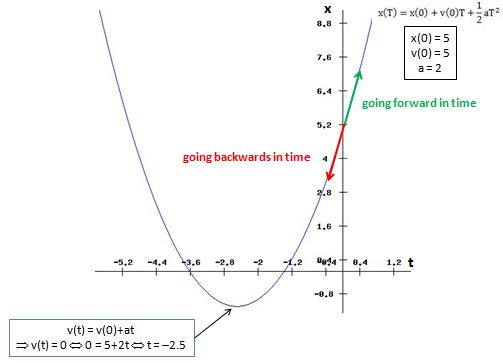
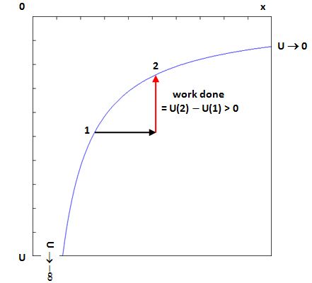
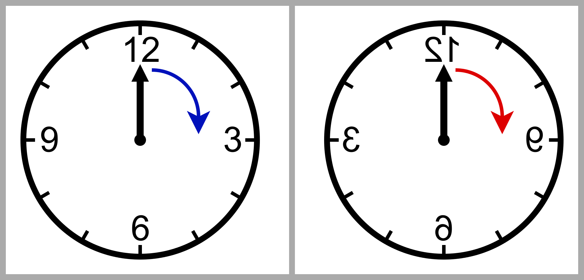
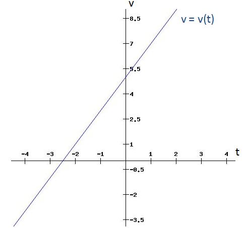
A ‘time reversal transformation’ amounts to inserting –t (minus t) instead of t in all of our equations describing trajectories or physical laws. Such transformation is illustrated below. The blue curve might represent a car or a rocket accelerating (in this particular example, we have a constant acceleration a = 2). The vertical axis measures the displacement (x) as a function of time (t). , and the red curve is its T-transformation. The two curves are each other’s mirror image, with the vertical axis (i.e. the axis measuring the displacement x) as the mirror axis.

This view of things is quite static and, hence, somewhat primitive I should say. However, we can make a number of remarks already. For example, we can see that the slope (of the tangent) of the red curve is negative. This slope is the velocity (v) of the particle: v = dx/dt. Hence, a T-transformation is said to negate the velocity variable (in classical physics that is), just like it negates the time variable. [The verb ‘to negate’ is used here in its mathematical sense: it means ‘to take the additive inverse of a number’ — but you’ll agree that’s too lengthy to be useful as an expression.]

Note that velocity (and mass) determines (linear and angular) momentum and, hence, a T-transformation will also negate p and l, i.e. the linear and angular momentum of a particle.

Such variables – i.e. variables that are negated by the T-transformation – are referred to as odd variables, as opposed to even variables, which are not impacted by the T-transformation: the position of the particle or object (x) is an example of an even variable, and the force acting on a particle (F) is not being negated either: it just remains what it is, i.e. an external force acting on some mass or some charge. The acceleration itself is another ‘even’ variable.

This all makes sense: why would the force or acceleration change? When we put a minus sign in front of the time variable, we are basically just changing the direction of an axis measuring an independent variable. In a way, the only thing that we are doing is introducing some non-standard way of measuring time, isn’t it? Instead of counting from 0 to T, we count from 0 to minus T.

Well… No. In this post, I want to discuss actual time reversal. Can we go back in time? Can we put a genie back into a bottle? Can we reverse all processes in Nature and, if not, why not?

Time reversal and time symmetry are two different things: doing a T-transformation is a mathematical operation; trying to reverse time is something real. Let’s take an example from kinematics to illustrate the matter.

Kinematics

Kinematics can be summed up in one equation, best known as Newton’s Second Law: F = ma = m(dv/dt) = d(mv)/dt. In words: the time-rate-of-change of a quantity called momentum (mv) is proportional to the force on an object. In other words: the acceleration (a) of an object is proportional to the force (F), and the factor of proportionality is the mass of the object (m). Hence, the mass of an object is nothing but a measure of its inertia.

The numbering of laws (first, second, etcetera) – usually combining some name of a scientist – is often quite arbitrary but, in this case (Newton’s Laws), one can really learn something from listing and discussing them in the right order:

Newton’s First Law is the principle of inertia: if there’s no (other) force acting on an object, it will just continue doing what it does–i.e. nothing or, else, move in some straight line according to the direction of its momentum (i.e. the product of its mass and its velocity)–or further engage with the force it was already engaged with.
Newton’s Second Law is the law of kinematics. In kinematics, we analyze the motion of an object without caring about the origin of the force causing the motion. So we just describe how some force impacts the motion of the object on which it is acting without asking any questions about the force itself. We’ve written this law above: F = ma.
Finally, Newton’s Third Law is the law of gravitation, which describes the origin, the nature and the strength of the gravitational force. That’s part of dynamics, i.e. the study of the forces themselves – as opposed to kinematics, which only looks at the motion caused by those forces.

With these definitions and clarifications, we are now well armed to tackle the subject of T-symmetry in kinematics (we’ll discuss dynamics later). Suppose some object – perhaps an elementary particle but it could also be a car or a rocket indeed – is moving through space with some constant acceleration a (so we can write a(t) = a). This means that v(t) – the velocity as a function of time – will not be constant: v(t) = at. [Note that we make abstraction of the direction here and, hence, our notation does not use any bold letters (which would denote vector quantities): v(t) and a(t) are just simple scalar quantities in this example.]

Of course, when we – i.e. you and me right here and right now – are talking time reversal, we obviously do it from some kind of vantage point. That vantage point will usually be the “now” (and quite often also the “here”), and so let’s use that as our reference frame indeed and we will refer to it as the zero time point: t = 0. So it’s not the origin of time: it’s just ‘now’–the start of our analysis.

Now, the idea of going back in time also implies the idea of looking forward – and vice versa. Let’s first do what we’re used to do and so that’s to look forward.

At some point in the future, let’s call it t = T, the velocity of our object will be equal to v(T) = v(0) + aT. Why the v(0)? Well… We defined the zero time point (t = 0) in a totally random way and, hence, our object is unlikely to stop for that. On the contrary: it is likely to already have some velocity and so that’s why we’re adding this v(0) here. As for the space coordinate, our object may also not be at the exact same spot as we are (we don’t want to be to close to a departing rocket I would assume), so we can also not assume that x(0) = 0 and so we will also incorporate that term somehow. It’s not essential to the analysis though.

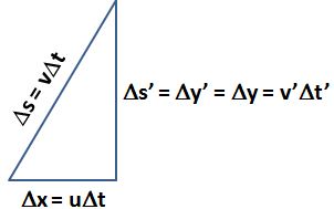
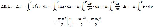
OK. Now we are ready to calculate the distance that our object will have traveled at point T. Indeed, you’ll remember that the distance traveled is an infinite sum of infinitesimally small products vΔt: the velocity at each point of time multiplied by an infinitesimally small interval of time. You’ll remember that we write such infinite sum as an integral:

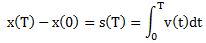
[In case you wonder why we use the letter ‘s’ for distance traveled: it’s because the ‘d’ symbol is already used to denote a differential and, hence, ‘s’ is supposed to stand for ‘spatium’, which is the Latin word for distance or space. As for the integral sign, you know that’s an elongated S really, don’t you? So its stands for an infinite sum indeed. But lets go back to the main story.]

We have a functional form for v(t), namely v(t) = v(0) + at, and so we can easily work out this integral to find s as a function of time. We get the following equation:

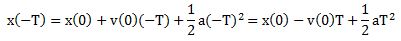
When we re-arrange this equation, we get the position of our object as a function of time:

Let us now reverse time by inserting –T everywhere:

Does that still make sense? Yes, of course, because we get the same result when doing our integral:

So that ‘makes sense’. However, I am not talking mathematical consistency when I am asking if it still ‘makes sense’. Let us interpret all of this by looking at what’s happening with the velocity. At t = 0, the velocity of the object is v(0), but T seconds ago, i.e. at point t = -T, the velocity of the object was v(-T) = v(0) – aT. This velocity is less than v(0) and, depending on the value of -T, it might actually be negative. Hence, when we’re looking back in time, we see the object decelerating (and we should immediately add that the deceleration is – just like the acceleration – a constant). In fact, it’s the very same constant a which determines when the velocity becomes zero and then, when going even further back in time, when it becomes negative.

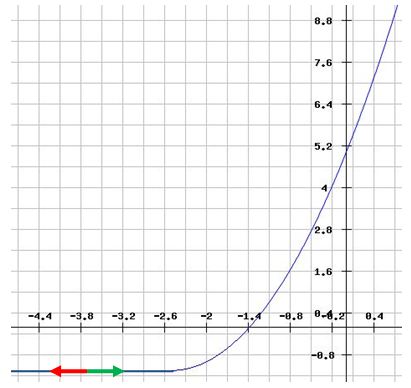
Huh? Negative velocity? Here’s the difference with the movie: in that movie that we are playing backwards, our car, our rocket, or the glass falling from a table or a pedestal would come to rest at some point back in time. We can calculate that point from our velocity equation v(t) = v(0) + at. In the example below, our object started accelerating 2.5 seconds ago, at point t = –2.5. But, unlike what we would see happening in our backwards-playing movie, we see that object not only stopping but also reversing its direction, to go in the same direction as we saw it going when we’re watching the movie before we hit the ‘Play Backwards’ button. So, yes, the velocity of our object changes sign as it starts following the trajectory on the left side of the graph.

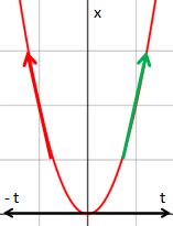
What’s going on here? Well… Rest assured: it’s actually quite simple: because the car or that rocket in our movie are real-life objects which were actually at rest before t = –2.5, the left side of the graph above is – quite simply – not relevant: it’s just a mathematical thing. So it does not depict the real-life trajectory of an accelerating car or rocket. The real-life trajectory of that car or rocket is depicted below.

So we also have a ‘left side’ here: a horizontal line representing no movement at all. Our movie may or may not have included this status quo. If it did, you should note that we would not be able to distinguish whether or not it would be playing forward or backwards. In fact, we wouldn’t be able to tell whether the movie was playing at all: we might just as well have hit the ‘pause’ button and stare at a frozen screenshot.

Does that make sense? Yes. There are no forces acting on this object here and, hence, there is no arrow of time.

Dynamics

The numerical example above is confusing because our mind is not only thinking about the trajectory as such but also about the force causing the particle—or the car or the rocket in the example above—to move in this or that direction. When it’s a rocket, we know it ignited its boosters 2.5 seconds ago (because that’s what we saw – in reality or in a movie of the event) and, hence, seeing that same rocket move backwards – both in time as well as in space – while its boosters operate at full thrust does not make sense to us. Likewise, an obstacle escaping gravity with no other forces acting on it does not make sense either.

That being said, reversing the trajectory and, hence, actually reversing the effects of time, should not be a problem—from a purely theoretical point at least: we should just apply twice the force produced by the boosters to give that rocket the same acceleration in the reverse direction. That would obviously means we would force it to crash back into the Earth. Because that would be rather complicated (we’d need twice as many boosters but mounted in the opposite direction), and because it would also be somewhat evil from a moral point of view, let us consider some less destructive examples.

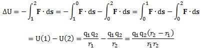
Let’s take gravity, or electrostatic attraction or repulsion. These two forces also cause uniform acceleration or deceleration on objects. Indeed, one can describe the force field of a large mass (e.g. the Earth)—or, in electrostatics, some positive or negative charge in space— using field vectors. The field vectors for the electric field are denoted by E, and, in his famous Lectures on Physics, Feynman uses a C for the gravitational field. The forces on some other mass m and on some other charge q can then be written as F = mC and F = qE respectively. The similarity with the F = ma equation – Newton’s Second Law in other words – is obvious, except that F = mC and F = qE are an expression of the origin, the nature and the strength of the force:

In the case of the electrostatic force (remember that likes repel and opposites attract), the magnitude of E is equal to E = q_c/4πε₀r². In this equation, ε₀is the electric constant, which we’ve encountered before, and r is the distance between the charge q and the charge q_ccausing the field).
For the gravitational field we have something similar, except that there’s only attraction between masses, no repulsion. The magnitude of C will be equal to C = –Gm_E/r², with m_E the mass causing the gravitational field (e.g. the mass of the Earth) and G the universal gravitational constant. [Note that the minus sign makes the direction of the force come out alright taking the existing conventions: indeed, it’s repulsion that gets the positive sign – but that should be of no concern to us here.]

So now we’ve explained the dynamics behind that x(t) = x(0) + v(0)·t + (a/2)·t²curve above, and it’s these dynamics that explain why looking back in time does not make sense—not in a mathematical way but in philosophical way. Indeed, it’s the nature of the force that gives time (or the direction of motion, which is the very same ‘arrow of time’) one–and only one–logical direction.

OK… But so what is time reversibility then – or time symmetry as it’s referred to? Let me defer an answer to this question by first introducing another topic.

Even and odd functions

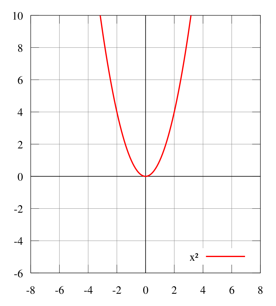
I already introduced the concept of even and odd variables above. It’s obviously linked to some symmetry/asymmetry. The x(t) curve above is symmetric. It is obvious that, if we would change our coordinate system to let x(0) equal x(0) = 0, and also choose the origin of time such that v(0) = 0, then we’d have a nice symmetry with respect to the vertical axis. The graph of the quadratic function below illustrates such symmetry.

Functions with a graph such as the one above are called even functions. A (real-valued) function f(t) of a (real) variable t is defined as even if, for all t and –t in the domain of f, we find that f(t) = f(–t).

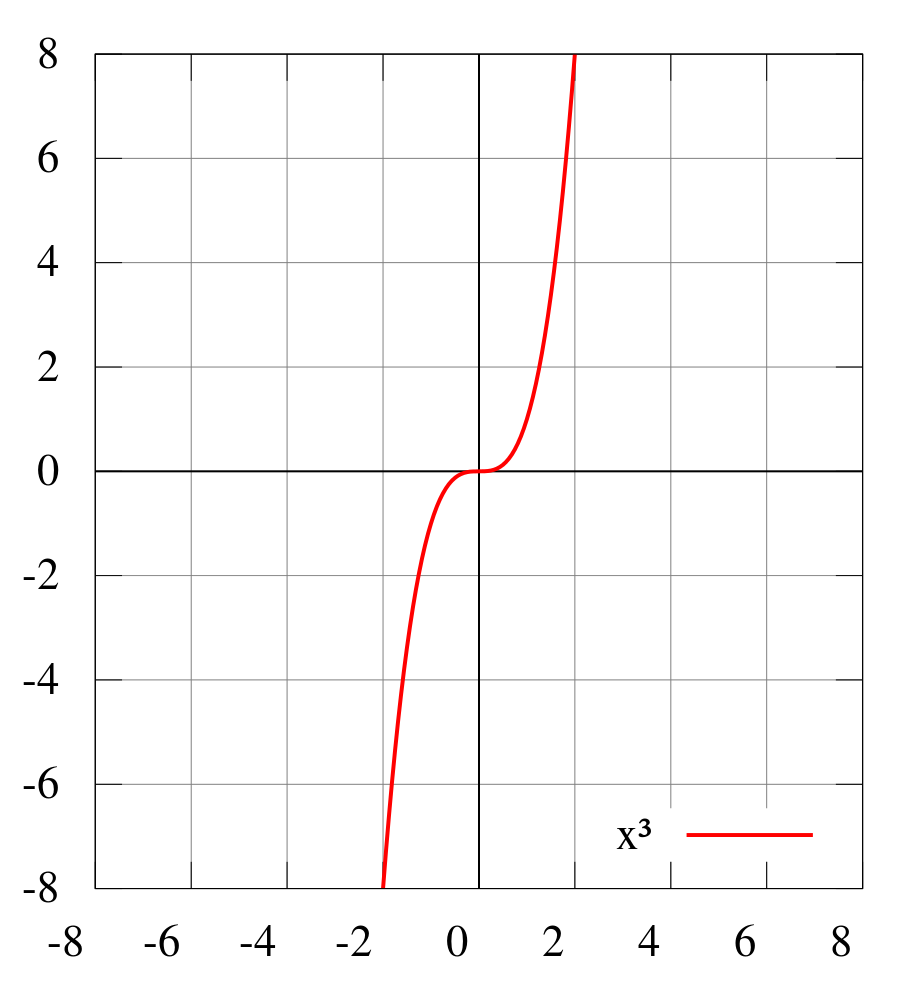
We also have odd functions, such as the one depicted below. An odd function is a function for which f(-t) = –f(t).

The function below gives the velocity as a function of time, and it’s clear that this would be an odd function if we would choose the zero time point such that v(0) = 0. In that case, we’d have a line through the origin and the graph would show an odd function. So that’s why we refer to v as an odd variable under time reversal.

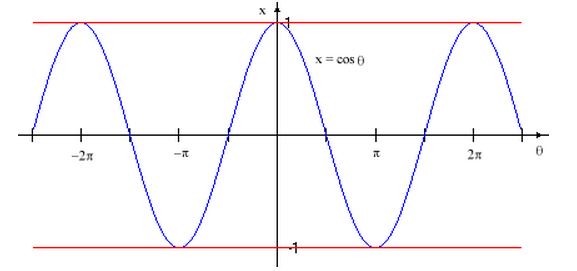
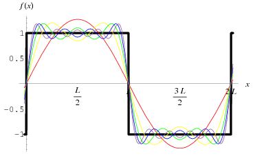
A very particular and very interesting example of an even function is the cosine function – as illustrated below.

Now, we said that the left side of the graph of the trajectory of our car or our rocket (i.e. the side with a negative slope and, hence, negative velocity) did not make much sense, because – as we play our movie backwards – it would depict a car or a rocket accelerating in the absence of a force. But let’s look at another situation here: a cosine function like the one above could actually represent the trajectory of a mass oscillating on a spring, as illustrated below.

In the case of a spring, the force causing the oscillation pulls back when the spring is stretched, and it pushes back when it’s compressed, so the mechanism is such that the direction of the force is being reversed continually. According to Hooke’s Law, this force is proportional to the amount of stretch. If x is the displacement of the mass m, and k that factor of proportionality, then the following equality must hold at all times:

F = ma = m(d²x/dt²) = –kx ⇔ d²x/dt²= –(k/m)x

Is there also a logical arrow of time here? Look at the illustration below. If we follow the green arrow, we can readily imagine what’s happening: the spring gets stretched and, hence, the mass on the spring (at maximum speed as it passes the equilibrium position) encounters resistance: the spring pulls it back and, hence, it slows down and then reverses direction. In the reverse direction – i.e. the direction of the red arrow – we have the reverse logic: the spring gets compressed (x is negative), the mass slows down (as evidence by the curvature of the graph), and – at some point – it also reverses its direction of movement. [I could note that the force equation above is actually a second-order linear differential equation, and that the cosine function is its solution, but that’s a rather pedantic and, hence, totally superfluous remark here.]

What’s important is that, in this case, the ‘arrow of time’ could point either way, and both make sense. In other words, when we would make a movie of this oscillating movement, we could play it backwards and it would still make sense.

Huh? Yes. Just in case you would wonder whether this conclusion depends on our starting point, it doesn’t. Just look at the illustration below, in which I assume we are starting to watch that movie (which is being played backwards without us knowing it is being played backwards) of the oscillating spring when the mass is not in the equilibrium position. It makes perfect sense: the spring is stretched, and we see the mass accelerating to the equilibrium position, as it should.

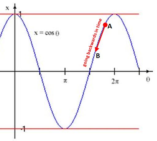
What’s going on here? Why can we reverse the arrow of time in the case of the spring, and why can’t we do that in the case of that particle being attracted or repelled by another? Are there two realities here? No. There’s only. I’ve been playing a trick on you. Just think about what is actually happening and then think about that so-called ‘time reversal’:

At point A, the spring is still being stretched further, in reality that is, and so the mass is moving away from the equilibrium position. Hence, in reality, it will not move to point B but further away from the equilibrium position.
However, we could imagine it moving from point A to B if we would reverse the direction of the force. Indeed, the force is equal to –kx and reversing its direction is equivalent to flipping our graph around the horizontal axis (i.e. the time axis), or to shifting the time axis left or right with an amount equal to π (note that the ‘time’ axis is actually represented by the phase, but that’s a minor technical detail and it does not change the analysis: we just measure time in radians here instead of seconds).

It’s a visual trick. There is no ‘real’ symmetry. The flipped graph corresponds to another situation (i.e. some other spring that started oscillating a bit earlier or later than ours here). Hence, our conclusion that it is the force that gives time direction, still holds.

Hmm… Let’s think about this. What makes our ‘trick’ work is that the force is allowed to change direction. Well… If we go back to our previous example of an object falling towards the center of some gravitational field, or a charge being attracted by some other (opposite) charge, then you’ll note that we can make sense of the ‘left side’ of the graph if we would change the sign of the force.

Huh? Yes, I know. This is getting complicated. But think about it. The graph below might represent a charged particle being repelled by another (stationary) particle: that’s the green arrow. We can then go back in time (i.e. we reverse the green arrow) if we reverse the direction of the force from repulsion to attraction. Now, that would usually lead to a dramatic event—the end of the story to be precise. Indeed, once the two particles get together, they’re glued together and so we’d have to draw another horizontal line going in the minus t direction (i.e. to the left side of our time axis) representing the status quo. Indeed, if the two particles sit right on top of each other, or if they would literally fuse or annihilate each other (like a particle and an anti-particle), then there’s no force or anything left at all… except if… we would alter the direction of the force once again, in which case the two particles would fly apart again (OK. OK. You’re right in noting that’s not true in the annihilation case – but that’s a minor detail).

Is this story getting too complicated? It shouldn’t. The point to note is that reversibility – i.e. time reversal in the philosophical meaning of the word (not that mathematical business of inserting negative variables instead of positive ones) – is all about changing the direction of the force: going back in time implies that we reverse the effects of time, and reversing the effects of time, requires forces acting in the opposite direction.

Now, when it’s only kinetic energy that is involved, then it should be easy but when charges are involved, which is the case for all fundamental forces, then it’s not so easy. That’s when charge (C) and parity (P) symmetry come into the picture.

CP symmetry

Hooke’s ‘Law’ – i.e. the law describing the force on a mass on a stretched or compressed spring – is not a fundamental law: eventually the spring will stop. Yes. It will stop even if when it’s in a horizontal position and with the mass moving on a frictionless surface, as assumed above: the forces between the atoms and/or molecules in the spring give the spring the elasticity which causes the mass to oscillate around some equilibrium position, but some of the energy of that continuous movement gets lost in heat energy (yes, an oscillating spring does actually get warmer!) and, hence, eventually the movement will peter out and stop.

Nevertheless, the lesson we learned above is a valuable one: when it comes to the fundamental forces, we can reverse the arrow of time and still make sense of it all if we also reverse the ‘charges’. The term ‘charges’ encompasses anything measuring a propensity to interact through one of the four fundamental forces here. That’s where CPT symmetry comes in: if we reverse time, we should also reverse the charges.

But how can we change the ‘sign’ of mass: mass is always positive, isn’t it? And what about the P-symmetry – this thing about left-handed and right-handed neutrinos?

Well… I don’t know. That’s the kind of stuff I am currently exploring in my quest. I’ll just note the following:

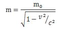
1. Gravity might be a so-called pseudo force – because it’s proportional to mass. I won’t go into the details of that – if only because I don’t master them as yet – but Einstein’s gut instinct that gravity is not a ‘real’ fundamental force (we just have to adjust our reference frame and work with curved spacetime) – and, hence, that ‘mass’ is not like the other force ‘charges’ – is something I want to further explore. [Apart from being a measure for inertia, you’ll remember that (rest) mass can also be looked at as equivalent to a very dense chunk of energy, as evidenced by Einstein’s energy-mass equivalence formula: E = mc².]

As for now, I can only note that the particles in an ‘anti-world’ would have the same mass. In that sense, anti-matter is not ‘anti’-matter: it just carries opposite electromagnetic, strong and weak charges. Hence, our C-world (so the world we get when applying a charge transformation) would have all ‘charges’ reversed, but mass would still be mass.

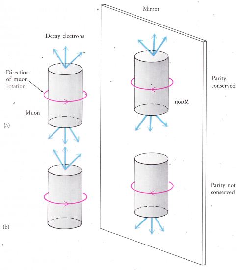
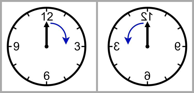
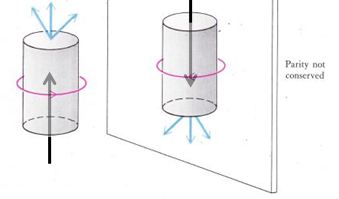
2. As for parity symmetry (i.e. left- and right-handedness, aka as mirror symmetry), I note that it’s raised primarily in relation to the so-called weak force and, hence, it’s also a ‘charge’ of sorts—in my primitive view of the world at least. The illustration below shows what P symmetry is all about really and may or may not help you to appreciate the point.

OK. What is this? Let’s just go step by step here.

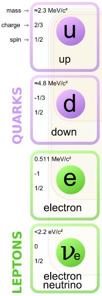
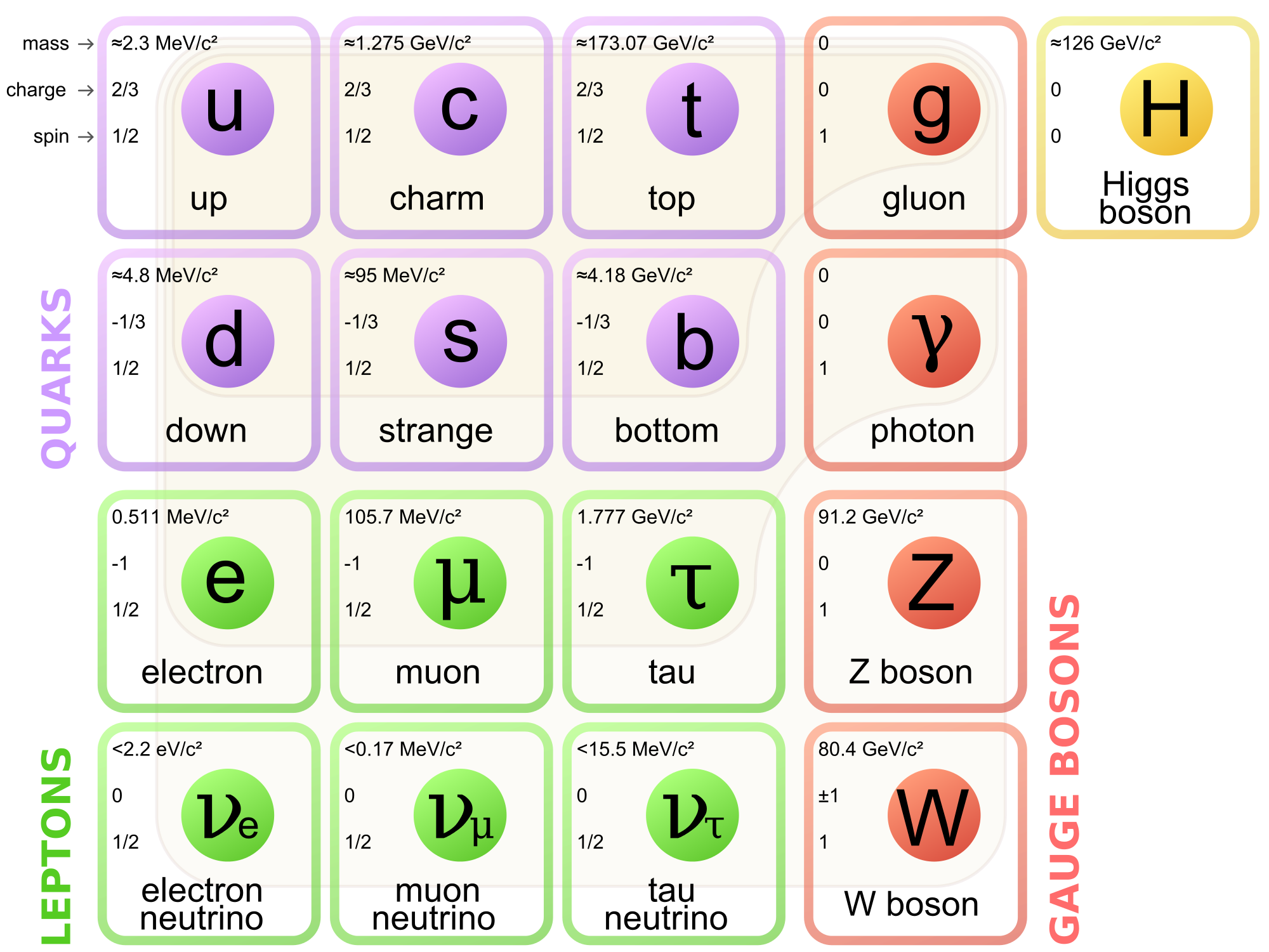
The ‘cylinder’ (both in (a), the upper part of the illustration, and in (b), the lower part) represents a muon—or a bunch of muons actually. A muon is an unstable particle in the lepton family. Think of it as a very heavy electron for all practical purposes: it’s about 200 times the mass of an electron indeed. Its lifetime is fairly short from our (human) point of view–only 2.2 microseconds on average–but that’s actually an eternity when compared to other unstable particles.

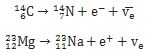
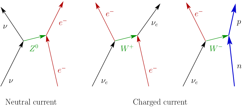
In any case, the point to note is that it usually decays into (i) two neutrinos (one muon-neutrino and one electron-antineutrino to be precise) and – importantly – (ii) one electron, so electric charge is preserved (indeed, neutrinos got the name they have because they carry no electric charge).

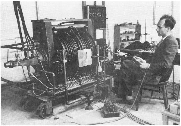
Now, we have left- and right-handed muons, and we can actually line them up in one of these two directions. I would need to check how that’s done, but muons do have a magnetic moment (just like electrons) and so I must assume it’s done in the same way as in Wu’s cobalt-60 experiment: through a uniform magnetic field. In other words, we know their spin directions in an experiment like this.

Now, if the weak force would respect mirror symmetry (but we already know it doesn’t), we would not be able to distinguish (i) the muon decay process in the ‘mirror world’ (i.e. the reflection of what’s going on in the (imaginary) mirror in the illustration above) from (ii) the decay process in ‘our’ (real) world. So that would be situation (a): the number of decay electrons being emitted in an upward direction would be the same (more or less) as the amount of decay electrons being emitted in a downward direction.

However, the actual laboratory experiments show that situation (b) is actually the case: most of the electrons are being emitted in only one direction (i.e. the upward direction in the illustration above) and, hence, the weak force does not respect mirror symmetry.

So what? Is that a problem?

For eminent physicists such as Feynman, it is. As he writes in his concluding Lecture on mechanics, radiation and heat (Vol. I, Chapter 52: Symmetry in Physical Laws): “It’s like seeing small hairs growing on the north pole of a magnet but not on its south pole.” [He means it allows us to distinguish the north and the south pole of a magnet in some absolute sense. Indeed, if we’re not able to tell right from left, we’re also not able to tell north from south – in any absolute sense that is. But so the experiment shows we actually can distinguish the two in some kind of absolute sense.]

I should also note that Wolfgang Pauli, one of the pioneers of quantum mechanics, said that it was “total nonsense” when he was informed about Wu’s experimental results, and that repeated experiments were needed to actually convince him that we cannot just create a mirror world out of ours.

For me, it is not a problem.I like to think of left- and right-handedness as some charge itself, and of the combined CPT symmetry as the only symmetry that matters really. That should be evident from my rather intuitive introduction on time symmetry above.

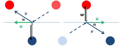
Consider it and decide for yourself how logical or illogical it is. We could define what Feynman refers to as an axial vector: watching that muon ‘from below’, we see that its spin is clockwise, and let’s use that fact to define an axial vector pointing in the same direction as the thick black arrow (it’s the so-called ‘right-hand screw rule’ really), as shown below.

Now, let’s suppose that mirror world actually exists, in some corner in the universe, and that a guy living in that ‘mirror world’ would use that very same ‘right-hand-screw rule’: his axial vector when doing this experiment would point in the opposite direction (see the thick black arrow in the mirror, which points in the opposite direction indeed). So what’s wrong with that?

Nothing – in my modest view at least. Left- and right-handedness can just be looked at as any other ‘charge’ – I think – and, hence, if we would be able to communicate with that guy in the ‘mirror world’, the two experiments would come out the same. So the other guy would also notice that the weak force does not respect mirror symmetry but so there’s nothing wrong with that: he and I should just get over it and continue to do business as usual, wouldn’t you agree?

After all, there could be a zillion reasons for the experiment giving the results it does: perhaps the ‘right-handed’ spin of the muon is sort of transferred to the electron as the muon decays, thereby giving it the same type of magnetic moment as the one that made the muon line up in the first place. Or – in a much wilder hypothesis which no serious physicist would accept – perhaps we actually do not yet understand everything of the weak decay process: perhaps we’ve got all these solar neutrinos (which all share the same spin direction) interfering in the process.

Whatever it is: Nature knows the difference between left and right, and I think there’s nothing wrong with that. Full stop.

But then what is ‘left’ and ‘right’ really? As the experiment pointed out, we can actually distinguish between the two in some kind of absolute sense. It’s not just a convention. As Feynman notes, we could decide to label ‘right’ as ‘left’, and ‘left’ as ‘right’ right here and right now – and impose the new convention everywhere – but then these physics experiments will always yield the same physical results, regardless of our conventions. So, while we’d put different stickers on the results, the laws of physics would continue to distinguish between left and right in the same absolute sense as Wu’s cobalt-60 decay experiment did back in 1956.

The really interesting thing in this rather lengthy discussion–in my humble opinion at least–is that imaginary ‘guy in the mirror world’. Could such mirror world exist? Why not? Let’s suppose it does really exist and that we can establish some conversation with that guy (or whatever other intelligent life form inhabiting that world).

We could then use these beta decay processes to make sure his ‘left’ and ‘right’ definitions are equal to our ‘left’ and ‘right’ definitions. Indeed, we would tell him that the muons can be left- or right-handed, and we would ask him to check his definition of ‘right-handed’ by asking him to repeat Wu’s experiment. And, then, when finally inviting him over and preparing to physically meet with him, we should tell him he should use his “right” hand to greet us. Yes. We should really do that.

Why? Well… As Feynman notes, he (or she or whatever) might actually be living in an anti-matter world, i.e. a world in which all charges are reversed, i.e. a world in which protons carry negative charge and electrons carry positive charge, and in which the quarks have opposite color charge. In that case, we would have been updating each other on all kinds of things in a zillion exchanges, and we would have been trying hard to assure each other that our worlds are not all that different (including that crucial experiment to make sure his left and right are the same as ours), but – if he would happen to live in an anti-matter world – then he would put out his left hand – not his right – when getting out of his spaceship. Touching it would not be wise. 🙂

[Let me be much more pedantic than Feynman is and just point out that his spaceship would obviously have been annihilated by ‘our’ matter long before he would have gotten to the meeting place. As soon as he’d get out of his ‘anti-matter’ world, we’d see a big flash of light and that would be it.]

Symmetries and conservation laws

A final remark should be made on the relation between all those symmetries and conservation laws. When everything is said and done, all that we’ve got is some nice graphs and then some axis or plane of symmetry (in two and three dimensions respectively). Is there anything more to it? There is.

There’s a “deep connection”, it seems, between all these symmetries and the various ‘laws of conservation’. In our examples of ‘time symmetry’, we basically illustrated the law of energy conservation:

When describing a particle traveling through an electrostatic or gravitation field, we basically just made the case that potential energy is converted into kinetic energy, or vice versa.
When describing an oscillating mass on a spring, we basically looked at the spring as a reservoir of energy – releasing and absorbing kinetic energy as the mass oscillates around its zero energy point – but, once again, all we described was a system in which the total amount of energy – kinetic and elastic – remained the same.

In fact, the whole discussion on CPT symmetry above has been quite simplistic and can be summarized as follows:

Energy is being conserved. Therefore, if you want to reverse time, you’ll need to reverse the forces as well. And reversing the forces implies a change of sign of the charges causing those forces.

In short, one should not be fascinated by T-symmetry alone. Combined CPT symmetry is much more intuitive as a concept and, hence, much more interesting. So, what’s left?

Quite a lot. I know you have many more questions at this point. At least I do:

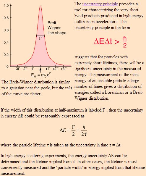
What does it mean in quantum mechanics? How does the Uncertainty Principle come into play?
How does it work exactly for the strong force, or for the weak force? [I guess I’d need to find out more about neutrino physics here…]
What about the other ‘conservation laws’ (such as the conservation of linear or angular momentum, for example)? How are they related to these ‘symmetries’.

Well… That’s complicated business it seems, and even Feynman doesn’t explore these topics in the above-mentioned final Lecture on (classical) mechanics. In any case, this post has become much too long already so I’ll just say goodbye for the moment. I promise I’ll get back to you on all of this.

Post scriptum:

If you have read my previous post (The Weird Force), you’ll wonder why – in the example of how a mirror world would relate to ours – I assume that the combined CP symmetry holds. Indeed, when discussing the ‘weird force’ (i.e. the weak force), I mentioned that it does not respect any of the symmetries, except for the combined CPT symmetry. So it does not respect (i) C symmetry, (ii) P symmetry and – importantly – it also does not respect the combined CP symmetry. This is a deep philosophical point which I’ll talk about in my next post. However, I needed this post as an ‘introduction’ to the next one.

The weird force

Pre-scriptum (dated 26 June 2020): While one of the illustrations in this post was removed as a result of an attack by the dark force, I am happy to see it still survived more or less intact. While my views on the true nature of light, matter and the force or forces that act on them have evolved significantly as part of my explorations of a more realist (classical) explanation of quantum mechanics, I think some of the analysis in this post remains fun to read. 🙂

Original post:

In my previous post (Loose Ends), I mentioned the weak force as the weird force. Indeed, unlike photons or gluons (i.e. the presumed carriers of the electromagnetic and strong force respectively), the weak force carriers (W bosons) have (1) mass and (2) electric charge:

W bosons are very massive. The equivalent mass of a W⁺and W^–boson is some 86.3 atomic mass units (amu): that’s about the same as a rubidium or strontium atom. The mass of a Z boson is even larger: roughly equivalent to the mass of a molybdenium atom (98 amu). That is extremely heavy: just compare with iron or silver, which have a mass of about 56 amu and 108 amu respectively. Because they are so massive, W bosons cannot travel very far before disintegrating (they actually go (almost) nowhere), which explains why the weak force is very short-range only, and so that’s yet another fundamental difference as compared to the other fundamental forces.
The electric charge of W and Z bosons explains why we have a trio of weak force carriers rather than just one: W⁺, W^–and Z⁰. Feynman calls them “the three W’s”.

The electric charge of W and Z bosons is what it is: an electric charge – just like protons and electrons. Hence, one has to distinguish it from the the weak charge as such: the weak charge (or, to be correct, I should say the weak isospin number) of a particle (such as a proton or a neutron for example) is related to the propensity of that particle to interact through the weak force — just like the electric charge is related to the propensity of a particle to interact through the electromagnetic force (think about Coulomb’s law for example: likes repel and opposites attract), and just like the so-called color charge (or the (strong) isospin number I should say) is related to the propensity of quarks (and gluons) to interact with each other through the strong force.

In short, as compared to the electromagnetic force and the strong force, the weak force (or Fermi’s interaction as it’s often called) is indeed the odd one out: these W bosons seem to mix just about everything: mass, charge and whatever else. In his 1985 Lectures on Quantum Electrodynamics, Feynman writes the following about this:

“The observed coupling constant for W’s is much the same as that for the photon. Therefore, the possibility exists that the three W’s and the photon are all different aspects of the same thing. Stephen Weinberg and Abdus Salam tried to combine quantum electrodynamics with what’s called ‘the weak interactions’ into one quantum theory, and they did it. But if you look at the results they get, you can see the glue—so to speak. It’s very clear that the photon and the three W’s are interconnected somehow, but at the present level of understanding, the connection is difficult to see clearly—you can still see the ‘seams’ in the theories; they have not yet been smoothed out so that the connection becomes more beautiful and, therefore, probably more correct.” (Feynman, 1985, p. 142)

Well… That says it all, I think. And from what I can see, the (tentative) confirmation of the existence of the Higgs field has not made these ‘seams’ any less visible. However, before criticizing eminent scientists such as Weinberg and Salam, we should obviously first have a closer look at those W bosons without any prejudice.

Alpha decay, potential wells and quantum tunneling

The weak force is usually explained as the force behind a process referred to as beta decay. However, because beta decay is just one form of radioactive decay, I need to say something about alpha decay too. [There is also gamma decay but that’s like a by-product of alpha and beta decay: when a nucleus emits an α or β particle (i.e. when we have alpha or beta decay), the nucleus will usually be left in an excited state, and so it can then move to a lower energy state by emitting a gamma ray photon (gamma radiation is very hard (i.e. very high-energy) radiation) – in the same way that an atomic electron can jump to a lower energy state by emitting a (soft) light ray photon. But so I won’t talk about gamma decay.]

Atomic decay, in general, is a loss of energy accompanying a transformation of the nucleus of the atom. Alpha decay occurs when the nucleus ejects an alpha particle: an α-particle consist of two protons and two neutrons bound together and, hence, it’s identical to a helium nucleus. Alpha particles are commonly emitted by all of the larger radioactive nuclei, such as uranium (which becomes thorium as a result of the decay process), or radium (which becomes radon gas). However, alpha decay is explained by a mechanism not involving the weak force: the electromagnetic force and the nuclear force (i.e. the strong force) will do. The reasoning is as follows: the alpha particle can be looked at as a stable but somewhat separate particle inside the nucleus. Because of their charge (both positive), the alpha particle inside of the nucleus and ‘the rest of the nucleus’ are subject to strong repulsive electromagnetic forces between them. However, these strong repulsive electromagnetic forces are not as strong as the strong force between the quarks that make up matter and, hence, that’s what keeps them together – most of the time that is.

Let me be fully complete here. The so-called nuclear force between composite particles such as protons and neutrons – or between clusters of protons and neutrons in this case – is actually the residual effect of the strong force. The strong force itself is between quarks – and between them only – and so that’s what binds them together in protons and neutrons (so that’s the next level of aggregation you might say). Now, the strong force is mostly neutralized within those protons and neutrons, but there is some residual force, and so that’s what keeps a nucleus together and what is referred to as the nuclear force.

There is a very helpful analogy here: the electromagnetic forces between neutral atoms (and/or molecules)—referred to as van der Waals forces (that’s what explains the liquid shape of water, among other things)— are also the residual of the (much stronger) electromagnetic forces that tie the electrons to the nucleus.

Now, that residual strong force – i.e. the nuclear force – diminishes in strength with distance but, within a certain distance, that residual force is strong enough to do what it does, and that’s to keep the nucleus together. This stable situation is usually depicted by what is referred to as a potential well:

The name is obvious: a well is a hole in the ground from which you can get water (or oil or gas or whatever). Now, the sea level might actually be lower than the bottom of a well, but the water would still stay in the well. In the illustration above, we are not depicting water levels but energy levels, but it’s equally obvious it would require some energy to kick a particle out of this well: if it would be water, we’d require a pump to get it out but, of course, it would be happy to flow to the sea once it’s out. Indeed, once a charged particle would be out (I am talking our alpha particle now), it will obviously stay out because of the repulsive electromagnetic forces coming into play (positive charges reject each other).

But so how can it escape the nuclear force and go up on the side of the well? [A potential pond or lake would have been a better term – but then that doesn’t sound quite right, does it? :-)]

Well, the energy may come from outside – that’s what’s referred to as induced radioactive decay (just Google it and you will tons of articles on experiments involving laser-induced accelerated alpha decay) – or, and that’s much more intriguing, the Uncertainty Principle comes into play.

Huh? Yes. According to the Uncertainty Principle, the energy of our alpha particle inside of the nucleus wiggles around some mean value but our alpha particle would also have an amplitude to have some higher energy level. That results not only in a theoretical probability for it to escape out of the well but also into something actually happening if we wait long enough: the amplitude (and, hence, the probability) is tiny, but it’s what explains the decay process – and what gives U-232 a half-life of 68.9 years, and also what gives the more common U-238 a much more comfortable 4.47 billion years as the half-life period.

[…]

Now that we’re talking about wells and all that, we should also mention that this phenomenon of getting out of the well is referred to as quantum tunneling. You can easily see why: it’s like the particle dug its way out. However, it didn’t: instead of digging under the sidewall, it sort of ‘climbed over’ it. Think of it being stuck and trying and trying and trying – a zillion times – to escape, until it finally did. So now you understand this fancy word: quantum tunneling. However, this post is about the weak force and so let’s discuss beta decay now.

Beta decay and intermediate vector bosons

Beta decay also involves transmutation of nuclei, but not by the emission of an α-particle but by a β-particle. A beta particle is just a different name for an electron (β^–) and/or its anti-matter counterpart: the positron (β⁺). [Physicists usually simplify stuff but in this case, they obviously didn’t: why don’t they just write e^– and e⁺here?]

An example of β⁻ decay is the decay of carbon-14 (C-14) into nitrogen-14 (N-14), and an example of β⁺ decay is the decay of magnesium-23 into sodium-23. C-14 and N-14 have the same mass but they are different atoms. The decay process is described by the equations below:

You’ll remember these formulas from your high-school days: beta decay does not change the mass number (carbon and nitrogen have the same mass: 14 units) but it does change the atomic (or proton) number: nitrogen has an extra proton. So one of the neutrons became a proton ! [The second equation shows the opposite: a proton became a neutron.] In order to do that, the carbon atom had to eject a negative charge: that’s the electron you see in the equation above.

In addition, there is also the ejection of a anti-neutrino (that’s what the bar above the v_e symbol stands for: antimatter). You’ll wonder what an antineutrino could possibly be. Don’t worry about it: it’s not any spookier than the neutrino. Neutrinos and anti-neutrinos have no electric charge and so you cannot distinguish them on that account (electric charge). However, all antineutrinos have right-handed helicity (i.e. they come in only one of the two possible spin states), while the neutrinos are all left-handed. That’s why beta-decay is said to not respect parity symmetry, aka as mirror symmetry. Hence, in the case of beta decay, Nature does distinguish between the world and the mirror world ! I’ll come back on that but let me first lighten up the discussion somewhat with a graphical illustration of that neutron-proton transformation.

As for magnesium-sodium transformation, we’d have something similar but so we’d just have a positron instead of an electron (a positron is just an electron with a positive charge for all practical purposes) and a regular neutrino. So we’d just have the anti-matter counterparts of the electron and the neutrino. [Don’t be put off by the term ‘anti-matter’: anti-matter is really just like regular matter – except that the charges have opposite sign. For example, the anti-matter counterpart of a blue quark is an anti-blue quark, and the anti-matter counterpart of neutrino has right-handed helicity – or spin – as opposed to the ‘left-handed’ ‘ordinary’ neutrinos.]

Now, you surely will have several serious questions. The most obvious question is what happens with the electron and the neutrino? Well… Those spooky neutrinos are gone before you know it and so don’t worry about them. As for the electron, the carbon had only six electrons but the nitrogen needs seven to be electrically neutral… So you might think the new atom will take care of it. Well… No. Sorry. Because of its kinetic energy, the electron is likely to just explore the world and crash into something else, and so we’re left with a positively charged nitrogen ion indeed. So I should have added a little ⁺sign next to the N in the formula above. Of course, one cannot exclude the possibility that this ion will pick up the electron later – but don’t bet on it: the ion might have to absorb another electron, or not find any free electrons !

As for the positron (in a β+ decay), that will just grab the nearest electron around and auto-destruct—thereby generating two high-energy photons (so that’s a little light flash). The net result is that we do not have an ion but a neutral sodium atom. Because the nearest electron will usually be found on some shell around the nucleus (the K or L shell for example), such process is often described as electron capture, and the ‘transformation equation’ can then be written p + e^–→ n + v_e (with p and n denoting a proton and a neutron respectively).

The more important question is: where are the W and Z bosons in this story?

Ah ! Yes! Sorry I forgot about them. The Feynman diagram below shows how it really works—and why the name of intermediate vector bosons for these three strange ‘particles’ (W⁺, W^–, and Z⁰) is so apt. These W bosons are just a short trace of ‘something’ indeed: their half-life is about 3×10⁻²⁵ s, and so that’s the same order of magnitude (or minitude I should say) as the mean lifetime of other resonances observed in particle collisions.

Indeed, you’ll notice that, in this so-called Feynman diagram, there’s no space axis. That’s because the distances involved are so tiny that we have to distort the scale—so we are not using equivalent time and distance units here, as Feynman diagrams should. That’s in line with a more prosaic description of what may be happening: W bosons mediate the weak force by seemingly absorbing an awful lot of momentum, spin, and whatever other energy related to all of the qubits describing the particles involved, to then eject an electron (or positron) and a neutrino (or an anti-neutrino).

Hmm… That’s not a standard description of a W boson as a force carrying particle, you’ll say. You’re right. This is more the description of a Z boson. What’s the Z boson again? Well… I haven’t explained it yet. It’s not involved in beta decay. There’s a process called elastic scattering of neutrinos. Elastic scattering means that some momentum is exchanged but neither the target (an electron or a nucleus) nor the incident particle (the neutrino) are affected as such (so there’s no break-up of the nucleus for example). In other words, things bounce back and/or get deflected but there’s no destruction and/or creation of particles, which is what you would have with inelastic collisions. Let’s examine what happens here.

W and Z bosons in neutrino scattering experiments

It’s easy to generate neutrino beams: remember their existence was confirmed in 1956 because nuclear reactors create a huge flux of them ! So it’s easy to send lots of high-energy neutrinos into a cloud or bubble chamber and see what happens. Cloud and bubble chambers are prehistoric devices which were built and used to detect electrically charged particles moving through it. I won’t go into too much detail but I can’t resist inserting a few historic pictures here.

The first two pictures below document the first experimental confirmation of the existence of positrons by Carl Anderson, back in 1932 (and, no, he’s not Danish but American), for which he got a Nobel Prize. The magnetic field which gives the positron some curvature—the trace of which can be seen in the image on the right—is generated by the coils around the chamber. Note the opening in the coils, which allows for taking a picture when the supersaturated vapor is suddenly being decompressed – and so the charged particle that goes through it leaves a trace of ionized atoms behind that act as ‘nucleation centers’ around which the vapor condenses, thereby forming tiny droplets. Quite incredible, isn’t it? One can only admire the perseverance of these early pioneers.

The picture below is another historical first: it’s the first detection of a neutrino in a bubble chamber. It’s fun to analyze what happens here: we have a mu-meson – aka as a muon – coming out of the collision here (that’s just a heavier version of the electron) and then a pion – which should (also) be electrically charged because the muon carries electric charge… But I will let you figure this one out. I need to move on with the main story. 🙂

The point to note is that these spooky neutrinos collide with other matter particles. In the image above, it’s a proton, but so when you’re shooting neutrino beams through a bubble chamber, a few of these neutrinos can also knock electrons out of orbit, and so that electron will seemingly appear out of nowhere in the image and move some distance with some kinetic energy (which can all be measured because magnetic fields around it will give the electron some curvature indeed, and so we can calculate its momentum and all that).

Of course, they will tend to move in the same direction – more or less at least – as the neutrinos that knocked them loose. So it’s like the Compton scattering which we discussed earlier (from which we could calculate the so-called classical radius of the electron – or its size if you will)—but with one key difference: the electrons get knocked loose not by photons, but by neutrinos.

But… How can they do that? Photons carry the electromagnetic field so the interaction between them and the electrons is electromagnetic too. But neutrinos? Last time I checked, they were matter particles, not bosons. And they carry no charge. So what makes them scatter electrons?

You’ll say that’s a stupid question: it’s the neutrino, dummy ! Yes, but how? Well, you’ll say, they collide—don’t they? Yes. But we are not talking tiny billiard balls here: if particles scatter, one of the fundamental forces of Nature must be involved, and usually it’s the electromagnetic force: it’s the electron density around nuclei indeed that explains why atoms will push each other away if they meet each other and, as explained above, it’s also the electromagnetic force that explains Compton scattering. So billiard balls bounce back because of the electromagnetic force too and…

OK-OK-OK. I got it ! So here it must be the strong force or something. Well… No. Neutrinos are not made of quarks. You’ll immediately ask what they are made of – but the answer is simple: they are what they are – one of the four matter particles in the Standard Model – and so they are not made of anything else. Capito?

OK-OK-OK. I got it ! It must be gravity, no? Perhaps these neutrinos don’t really hit the electron: perhaps they skim near it and sort of drag it along as they pass? No. It’s not gravity either. It can’t be. We have no exact measurement of the mass of a neutrino but it’s damn close to zero – and, hence, way too small to exert any such influence on an electron. It’s just not consistent with those traces.

OK-OK-OK. I got it ! It’s that weak force, isn’t it? YES ! The Feynman diagrams below show the mechanism involved. As far as terminology goes (remember Feynman’s complaints about the up, down, strange, charm, beauty and truths quarks?), I think this is even worse. The interaction is described as a current, and when the neutral Z boson is involved, it’s called a neutral current – as opposed to… Well… Charged currents. Neutral and charged currents? That sounds like sweet and sour candy, isn’t it? But isn’t candy supposed to be sweet? Well… No. Sour candy is pretty common too. And so neutral currents are pretty common too.

You obviously don’t believe a word of what I am saying and you’ll wonder what the difference is between these charged and neutral currents. The end result is the same in the first two pictures: an electron and a neutrino interact, and they exchange momentum. So why is one current neutral and the other charged? In fact, when you ask that question, you are actually wondering whether we need that neutral Z boson. W bosons should be enough, no?

No. The first and second picture are “the same but different”—and you know what that means in physics: it means it’s not the same. It’s different. Full stop. In the second picture, there is electron absorption (only for a very brief moment obviously, but so that’s what it is, and you don’t have that in the first diagram) and then electron emission, and there’s also neutrino absorption and emission. […] I can sense your skepticism – and I actually share it – but that’s what I understand of it !

[…] So what’s the third picture? Well… That’s actually beta decay: a neutron becomes a proton, and there’s emission of an electron and… Hey ! Wait a minute ! This is interesting: this is not what we wrote above: we have an incoming neutrino instead of an outgoing anti-neutrino here. So what’s this?

Well… I got this illustration from a blog on physics (Galileo’s Pendulum – The Flavor of Neutrinos) which, in turn, mentions Physics Today as its source. The incoming neutrino has nothing to do with the usual representation of an anti-matter particle as a particle traveling backwards in time. It’s something different, and it triggers a very interesting question: could beta decay possibly be ‘triggered’ by neutrinos? Who knows?

I googled it, and there seems to be some evidence supporting such thesis. However, this ‘evidence’ is flimsy (the only real ‘clue’ is that the activity of the Sun, as measured by the intensity of solar flares, seems to be having some (tiny) impact on the rate of decay of radioactive elements on Earth) and, hence, most ‘serious’ scientists seem to reject that possibility. I wonder why: it would make the ‘weird force’ somewhat less weird in my view. So… What to say? Well… Nothing much at this moment. Let me move on and examine the question a bit more in detail in a Post Scriptum.

The odd one out

You may wonder if neutrino-electron interaction always involve the weak force. The answer to that question is simple: Yes ! Because they do not carry any electric charge, and because they are not quarks, neutrinos are only affected by the weak force. However, as evidenced by all the stuff I wrote on beta decay, you cannot turn this statement on its head: the weak force is relevant not only for neutrinos but for electrons and quarks as well ! That gives us the following connection between forces and matter:

[Specialists reading this post may say they’ve not seen this diagram before. That might be true. I made it myself – for a change – but I am sure it’s around somewhere.]

It is a weird asymmetry: almost massless particles (neutrinos) interact with other particles through massive bosons, and these massive ‘things’ are supposed to be ‘bosons’, i.e. force carrying particles ! These physicists must be joking, right? These bosons can hardly carry themselves – as evidenced by the fact they peter out just like all of those other ‘resonances’ !

Hmm… Not sure what to say. It’s true that their honorific title – ‘intermediate vectors’ – seems to be quite apt: they are very intermediate indeed: they only appear as a short-lived stage in between the initial and final state of the system. Again, it leads one to think that these W bosons may just reflect some kind of energy blob caused by some neutrino – or anti-neutrino – crashing into another matter particle (a quark or an electron). Whatever it is, this weak force is surely the odd one out.

In my previous post, I mentioned other asymmetries as well. Let’s revisit them.

Time irreversibility

In Nature, uranium is usually found as uranium-238. Indeed, that’s the most abundant isotope of uranium: about 99.3% of all uranium is U-238. There’s also some uranium-235 out there: some 0.7%. And there are also trace amounts of U-234. And that’s it really. So where is the U-232 we introduced above when talking about alpha decay? Well… We said it has a half-life of 68.9 years only and so it’s rather normal U-232 cannot be found in Nature. What? Yes: 68.9 years is nothing compared to the half-life of U-238 (4.47 billion years) or U-235 (704 million years), and so it’s all gone. In fact, the tiny proportion of U-235 on this Earth is what allows us to date the Earth. The math and physics involved resemble the math and physics involved in carbon-dating but so carbon-dating is used for organic materials only, because the carbon-14 that’s used also has a fairly short half-time: 5,730 years—so that’s like a thousand times more than U-232 but… Well… Not like millions or billions of years. [You’ll immediately ask why this C-14 is still around if it’s got such a short life-time. The answer to that is easy: C-14 is continually being produced in the atmosphere and, hence, unlike U-232, it doesn’t just disappear.]

Hmm… Interesting. Radioactive decay suggests time irreversibility. Indeed, it’s wonderful and amazing – but sad at the same time:

There’s so much diversity – a truly incredible range of chemical elements making life what it is.
But so all these chemical elements have been produced through a process of nuclear fusion in stars (stellar nucleosynthesis), which were then blasted into space by supernovae, and so they then coagulated into planets like ours.
However, all of the heavier atoms will decay back into some lighter element because of radioactive decay, as shown in the graph below.
So we are doomed !

Overview of decay modes

In fact, some of the GUT theorists think that there is no such thing as ‘stable nuclides’ (that’s the black line in the graph above): they claim that all atomic species will decay because – according to their line of reasoning – the proton itself is NOT stable.

WHAT? Yeah ! That’s what Feynman complained about too: he obviously doesn’t like these GUT theorists either. Of course, there is an expensive experiment trying to prove spontaneous proton decay: the so-called Super-K under Mount Kamioka in Japan. It’s basically a huge tank of ultra-pure water with a lot of machinery around it… Just google it. It’s fascinating. If, one day, it would be able to prove that there’s proton decay, our Standard Model would be in very serious problems – because it doesn’t cater for unstable protons. That being said, I am happy that has not happened so far – because it would mean our world would really be doomed.

What do I mean with that? We’re all doomed, aren’t we? If only because of the Second Law of Thermodynamics. Huh? Yes. That ‘law’ just expresses a universal principle: all kinetic and potential energy observable in nature will, in the end, dissipate: differences in temperature, pressure, and chemical potential will even out. Entropy increases. Time is NOT reversible: it points in the direction of increasing entropy – till all is the same once again. Sorry?

Don’t worry about it. When everything is said and done, we humans – or life in general – are an amazing negation of the Second Law of Thermodynamics: temperature, pressure, chemical potential and what have you – it’s all super-organized and super-focused in our body ! But it’s temporary indeed – and we actually don’t negate the Second Law of Thermodynamics: we create order by creating disorder. In any case, I don’t want to dwell on this point. Time reversibility in physics usually refers to something else: time reversibility would mean that all basic laws of physics (and with ‘basic’, I am excluding this higher-level Second Law of Thermodynamics) would be time-reversible: if we’d put in minus t (–t) instead of t, all formulas would still make sense, wouldn’t they? So we could – theoretically – reverse our clock and stopwatches and go back in time.

Can we do that?

Well… We can reverse a lot. For example, U-232 decays into a lot of other stuff BUT we can produce U-232 from scratch once again—from thorium to be precise. In fact, that’s how we got it in the first place: as mentioned above, any natural U-232 that might have been produced in those stellar nuclear fusion reactors is gone. But so that means that alpha decay is reversible: we’re producing stable stuff – U-232 lasts for dozens of years – that probably existed long time ago but so it decayed and now we’re reversing the arrow of time using our nuclear science and technology.

Now, you may object that you don’t see Nature spontaneously assemble the nuclear technology we’re using to produce U-232, except if Nature would go for that Big Crunch everyone’s predicting so it can repeat the Big Bang once again (so that’s the oscillating Universe scenario)—and you’re obviously right in that assessment. That being said, from some kind of weird existential-philosophical point of view, it’s kind of nice to know that – in theory at least – there is time reversibility indeed (or T symmetry as it’s called by scientists).

[Voice booming from the sky] STOP DREAMING ! TIME REVERSIBILITY DOESN’T EXIST !

What? That’s right. For beta decay, we don’t have T symmetry. The weak force breaks all kinds of symmetries, and time symmetry is only one of them. I talked about these in my previous post (Loose Ends) – so please have a look at that, and let me just repeat the basics:

Parity (P) symmetry or mirror symmetry revolves around the notion that Nature should not distinguish between right- and left-handedness, so everything that works in our world, should also work in the mirror world. Now, the weak force does not respect P symmetry: we need right-handed neutrinos for β^– decay, and we’d also need right-handed neutrinos to reverse the process – which actually happens: so, yes, beta decay might be time-reversible but so it doesn’t work with left-handed neutrinos – which is what our ‘right-handed’ neutrinos would be in the ‘mirror world’. Full stop. Our world is different from the mirror world because the weak force knows the difference between left and right – and some stuff only works with left-handed stuff (and then some other stuff only works with right-handed stuff). In short, the weak force doesn’t work the same in the mirror world. In the mirror world, we’d need to throw in left-handed neutrinos for β^– decay. Not impossible but a bit of a nuisance, you’ll agree.
Charge conjugation or charge (C) symmetry revolves around the notion that a world in which we reverse all (electric) charge signs. Now, the weak force also does not respect C symmetry. I’ll let you go through the reasoning for that, but it’s the same really. Just reversing all signs would not make the weak force ‘work’ in the mirror world: we’d have to ‘keep’ some of the signs – notably those of our W bosons !
Initially, it was thought that the weak force respected the combined CP symmetry (and, therefore, that the principle of P and C symmetry could be substituted by a combined CP symmetry principle) but two experimenters – Val Fitch and James Cronin – got a Nobel Prize when they proved that this was not the case. To be precise, the spontaneous decay of neutral kaons (which is a type of decay mediated by the weak force) does not respect CP symmetry. Now, that was the death blow to time reversibility (T symmetry). Why? Can’t we just make a film of those experiments not respecting P, C or CP symmetry, and then just press the ‘reverse’ button? We could but one can show that the relativistic invariance in Einstein’s relativity theory implies a combined CPT symmetry. Hence, if CP is a broken symmetry, then the T symmetry is also broken. So we could play that film, but the laws of physics would not make sense ! In other words, the weak force does not respect T symmetry either !

To summarize this rather lengthy philosophical digression: a full CPT sequence of operations would work. So we could – in sequence – (1) change all particles to antiparticles (C), (2) reflect the system in a mirror (P), and (3) change the sign of time (T), and we’d have a ‘working’ anti-world that would be just as real as ours. HOWEVER, we do not live in a mirror world. We live in OUR world – and so left-handed is left-handed, and right-handed is right-handed, and positive is positive and negative is negative, and so THERE IS NO TIME REVERSIBILITY: the weak force does not respect T symmetry.

Do you understand now why I call the weak force the weird force? Penrose devotes a whole chapter to time reversibility in his Road to Reality, but he does not focus on the weak force. I wonder why. All that rambling on the Second Law of Thermodynamics is great – but one should relate that ‘principle’ to the fundamental forces and, most notably, to the weak force.

Post scriptum 1:

In one of my previous posts, I complained about not finding any good image of the Higgs particle. The problem is that these super-duper particle accelerators don’t use bubble chambers anymore. The scales involved have become incredibly small and so all that we have is electronic data, it seems, and that is then re-assembled into some kind of digital image but – when everything is said and done – these images are only simulations. Not the real thing. I guess I am just an old grumpy guy – a 45-year old economist: what do you expect? – but I’ll admit that those black-and-white pictures above make my heart race a bit more than those colorful simulations. But so I found a good simulation. It’s the cover image of Wikipedia’s Physics beyond the Standard Model (I should have looked there in the first place, I guess). So here it is: the “simulated Large Hadron Collider CMS particle detector data depicting a Higgs boson (produced by colliding protons) decaying into hadron jets and electrons.”

So that’s what gives mass to our massive W bosons. The Higgs particle is a massive particle itself: an estimated 125-126 GeV/c², so that’s about 1.5 times the mass of the W bosons. I tried to look into decay widths and all that, but it’s all quite confusing. In short, I have no doubt that the Higgs theory is correct – the data is all what we have and then, when everything is said and done, we have an honorable Nobel Prize Committee thinking the evidence is good enough (which – in light of their rather conservative approach (which I fully subscribe too: don’t get me wrong !) – usually means that it’s more than good enough !) – but I can’t help thinking this is a theory which has been designed to match experiment.

Wikipedia writes the following about the Higgs field:

“The Higgs field consists of four components, two neutral ones and two charged component fields. Both of the charged components and one of the neutral fields are Goldstone bosons, which act as the longitudinal third-polarization components of the massive W+, W– and Z bosons. The quantum of the remaining neutral component corresponds to (and is theoretically realized as) the massive Higgs boson.”

Hmm… So we assign some qubits to W bosons (sorry for the jargon: I am talking these ‘longitudinal third-polarization components’ here), and to W bosons only, and then we find that the Higgs field gives mass to these bosons only? I might be mistaken – I truly hope so (I’ll find out when I am somewhat stronger in quantum-mechanical math) – but, as for now, it all smells somewhat fishy to me. It’s all consistent, yes – and I am even more skeptical about GUT stuff ! – but it does look somewhat artificial.

But then I guess this rather negative appreciation of the mathematical beauty (or lack of it) of the Standard Model is really what is driving all these GUT theories – and so I shouldn’t be so skeptical about them ! 🙂

Oh… And as I’ve inserted some images of collisions already, let me insert some more. The ones below document the discovery of quarks. They come out of the above-mentioned coffee table book of Lederman and Schramm (1989). The accompanying texts speak for themselves.

Post scriptum 2:

I checked the source of that third diagram showing how an incoming neutrino could possibly cause a neutron to become a proton. It comes out of the August 2001 issue of Physics Today indeed, and it describes a very particular type of beta decay. This is the original illustration:

The article (and the illustration above) describes how solar neutrinos traveling through heavy water – also known as deuterium – can interact with the deuterium nucleus – which is referred to as deuteron, and which we’ll represent by the symbol d in the process descriptions below. The nucleus of deuterium – which is an isotope of hydrogen – consists of one proton and one neutron, as opposed to the much more common protium isotope of hydrogen, which has just one proton in the nucleus. Deuterium occurs naturally (0.0156% of all hydrogen atoms in the Earth’s oceans is deuterium), but it can also be produced industrially – for use in heavy-water nuclear reactors for example. In any case, the point is that deuteron can respond to solar neutrinos by breaking up in one of two ways:

Quasi-elastically: v_e + d → v_e + p + n. So, in this case, the deuteron just breaks up in its two components: one proton and one neutron. That seems to happen pretty frequently because the nuclear forces holding the proton and the neutron together are pretty weak it seems.
Alternatively, the solar neutrino can turn a deuteron’s neutron into a second proton, and so that’s what’s depicted in the third diagram above: v_e + d → e⁻ + p + p. So what happens really is v_e + n → e⁻ + p.

The author of this article – which basically presents the basics of how a new neutrino detector – the Sudbury Neutrino Observatory – is supposed to work – refers to the second process as inverse beta decay – but that’s a rather generic and imprecise term it seems. The conclusion is that the weak force seems to have myriad ways of expressing itself. However, the connection between neutrinos and the weak force seems to need further exploring. As for myself, I’d like to know why the hypothesis that any form of beta decay – or, for that matter, any other expression of the weak force – is actually being triggered by these tiny neutrinos crashing into (other) matter particles would not be reasonable.

In such scenario, the W bosons would be reduced to a (very) temporary messy ‘blob’ of energy, combining kinetic, electromagnetic as well as the strong binding energy between quarks if protons and neutrons are involved. Could this ‘odd one out’ be nothing but a pseudo-force? I am no doubt being very simplistic here – but then it’s an interesting possibility, isn’t it? In order to firmly deny it, I’ll need to learn a lot more about neutrinos no doubt – and about how the results of all these collisions in particle accelerators are actually being analyzed and interpreted.

Some content on this page was disabled on June 20, 2020 as a result of a DMCA takedown notice from Michael A. Gottlieb, Rudolf Pfeiffer, and The California Institute of Technology. You can learn more about the DMCA here:

https://wordpress.com/support/copyright-and-the-dmca/

Loose ends…

Pre-scriptum (dated 26 June 2020): My views on the true nature of light, matter and the force or forces that act on them have evolved significantly as part of my explorations of a more realist (classical) explanation of quantum mechanics. If you are reading this, then you are probably looking for not-to-difficult reading. In that case, I would suggest you read my re-write of Feynman’s introductory lecture to QM. If you want something shorter, you can also read my paper on what I believe to be the true Principles of Physics. Having said that, I still think there are a few good quotes and thoughts in this post too. 🙂

Original post:

It looks like I am getting ready for my next plunge into Roger Penrose’s Road to Reality. I still need to learn more about those Hamiltonian operators and all that, but I can sort of ‘see’ what they are supposed to do now. However, before I venture off on another series of posts on math instead of physics, I thought I’d briefly present what Feynman identified as ‘loose ends’ in his 1985 Lectures on Quantum Electrodynamics – a few years before his untimely death – and then see if any of those ‘loose ends’ appears less loose today, i.e. some thirty years later.

The three-forces model and coupling constants

All three forces in the Standard Model (the electromagnetic force, the weak force and the strong force) are mediated by force carrying particles: bosons. [Let me talk about the Higgs field later and – of course – I leave out the gravitational force, for which we do not have a quantum field theory.]

Indeed, the electromagnetic force is mediated by the photon; the strong force is mediated by gluons; and the weak force is mediated by W and/or Z bosons. The mechanism is more or less the same for all. There is a so-called coupling (or a junction) between a matter particle (i.e. a fermion) and a force-carrying particle (i.e. the boson), and the amplitude for this coupling to happen is given by a number that is related to a so-called coupling constant.

Let’s give an example straight away – and let’s do it for the electromagnetic force, which is the only force we have been talking about so far. The illustration below shows three possible ways for two electrons moving in spacetime to exchange a photon. This involves two couplings: one emission, and one absorption. The amplitude for an emission or an absorption is the same: it’s –j. So the amplitude here will be (–j)(–j) = j². Note that the two electrons repel each other as they exchange a photon, which reflects the electromagnetic force between them from a quantum-mechanical point of view !

We will have a number like this for all three forces. Feynman writes the coupling constant for the electromagnetic force as j and the coupling constant for the strong force (i.e. the amplitude for a gluon to be emitted or absorbed by a quark) as g. [As for the weak force, he is rather short on that and actually doesn’t bother to introduce a symbol for it. I’ll come back on that later.]

The coupling constant is a dimensionless number and one can interpret it as the unit of ‘charge’ for the electromagnetic and strong force respectively. So the ‘charge’ q of a particle should be read as q times the coupling constant. Of course, we can argue about that unit. The elementary charge for electromagnetism was or is – historically – the charge of the proton (q = +1), but now the proton is no longer elementary: it consists of quarks with charge –1/3 and +2/3 (for the d and u quark) respectively (a proton consists of two u quarks and one d quark, so you can write it as uud). So what’s j then? Feynman doesn’t give its precise value but uses an approximate value of –0.1. It is an amplitude so it should be interpreted as a complex number to be added or multiplied with other complex numbers representing amplitudes – so –0.1 is “a shrink to about one-tenth, and half a turn.” [In these 1985 Lectures on QED, which he wrote for a lay audience, he calls amplitudes ‘arrows’, to be combined with other ‘arrows.’ In complex notation, –0.1 = 0.1e^iπ= 0.1(cosπ + isinπ).]

Let me give a precise number. The coupling constant for the electromagnetic force is the so-called fine-structure constant, and it’s usually denoted by the alpha symbol (α). There is a remarkably easy formula for α, which becomes even easier if we fiddle with units to simplify the matter even more. Let me paraphrase Wikipedia on α here, because I have no better way of summarizing it (the summary is also nice as it shows how changing units – replacing the SI units by so-called natural units – can simplify equations):

1. There are three equivalent definitions of α in terms of other fundamental physical constants:

\alpha = \frac{k_\mathrm{e} e^2}{\hbar c} = \frac{1}{(4 \pi \varepsilon_0)} \frac{e^2}{\hbar c} = \frac{e^2 c \mu_0}{2 h}

where e is the elementary charge (so that’s the electric charge of the proton); ħ = h/2π is the reduced Planck constant; c is the speed of light (in vacuum); ε₀ is the electric constant (i.e. the so-called permittivity of free space); µ₀ is the magnetic constant (i.e. the so-called permeability of free space); and k_e is the Coulomb constant.

2. In the old centimeter-gram-second variant of the metric system (cgs), the unit of electric charge is chosen such that the Coulomb constant (or the permittivity factor) equals 1. Then the expression of the fine-structure constant just becomes:

\alpha = \frac{e^2}{\hbar c}

3. When using so-called natural units, we equate ε₀ , c and ħ to 1. [That does not mean they are the same, but they just become the unit for measurement for whatever is measured in them. :-)] The value of the fine-structure constant then becomes:

\alpha = \frac{e^2}{4 \pi}.

Of course, then it just becomes a matter of choosing a value for e. Indeed, we still haven’t answered the question as to what we should choose as ‘elementary’: 1 or 1/3? If we take 1, then α is just a bit smaller than 0.08 (around 0.0795775 to be somewhat more precise). If we take 1/3 (the value for a quark), then we get a much smaller value: about 0.008842 (I won’t bother too much about the rest of the decimals here). Feynman’s (very) rough approximation of –0.1 obviously uses the historic proton charge, so e = +1.

The coupling constant for the strong force is much bigger. In fact, if we use the SI units (i.e. one of the three formulas for α under point 1 above), then we get an alpha equal to some 7.297×10^–3. In fact, its value will usually be written as 1/α, and so we get a value of (roughly) 1/137. In this scheme of things, the coupling constant for the strong force is 1, so that’s 137 times bigger.

Coupling constants, interactions, and Feynman diagrams

So how does it work? The Wikipedia article on coupling constants makes an extremely useful distinction between the kinetic part and the proper interaction part of an ‘interaction’. Indeed, before we just blindly associate qubits with particles, it’s probably useful to not only look at how photon absorption and/or emission works, but also at how a process as common as photon scattering works (so we’re talking Compton scattering here – discovered in 1923, and it earned Compton a Nobel Prize !).

The illustration below separates the kinetic and interaction part properly: the photon and the electron are both deflected (i.e. the magnitude and/or direction of their momentum (p) changes) – that’s the kinetic part – but, in addition, the frequency of the photon (and, hence, its energy – cf. E = hν) is also affected – so that’s the interaction part I’d say.

With an absorption or an emission, the situation is different, but it also involves frequencies (and, hence, energy levels), as show below: an electron absorbing a higher-energy photon will jump two or more levels as it absorbs the energy by moving to a higher energy level (i.e. a so-called excited state), and when it re-emits the energy, the emitted photon will have higher energy and, hence, higher frequency.

This business of frequencies and energy levels may not be so obvious when looking at those Feynman diagrams, but I should add that these Feynman diagrams are not just sketchy drawings: the time and space axis is precisely defined (time and distance are measured in equivalent units) and so the direction of travel of particles (photons, electrons, or whatever particle is depicted) does reflect the direction of travel and, hence, conveys precious information about both the direction as well as the magnitude of the momentum of those particles. That being said, a Feynman diagram does not care about a photon’s frequency and, hence, its energy (its velocity will always be c, and it has no mass, so we can’t get any information from its trajectory).

Let’s look at these Feynman diagrams now, and the underlying force model, which I refer to as the boson exchange model.

The boson exchange model

The quantum field model – for all forces – is a boson exchange model. In this model, electrons, for example, are kept in orbit through the continuous exchange of (virtual) photons between the proton and the electron, as shown below.

Now, I should say a few words about these ‘virtual’ photons. The most important thing is that you should look at them as being ‘real’. They may be derided as being only temporary disturbances of the electromagnetic field but they are very real force carriers in the quantum field theory of electromagnetism. They may carry very low energy as compared to ‘real’ photons, but they do conserve energy and momentum – in quite a strange way obviously: while it is easy to imagine a photon pushing an electron away, it is a bit more difficult to imagine it pulling it closer, which is what it does here. Nevertheless, that’s how forces are being mediated by virtual particles in quantum mechanics: we have matter particles carrying charge but neutral bosons taking care of the exchange between those charges.

In fact, note how Feynman actually cares about the possibility of one of those ‘virtual’ photons briefly disintegrating into an electron-positron pair, which underscores the ‘reality’ of photons mediating the electromagnetic force between a proton and an electron, thereby keeping them close together. There is probably no better illustration to explain the difference between quantum field theory and the classical view of forces, such as the classical view on gravity: there are no gravitons doing for gravity what photons are doing for electromagnetic attraction (or repulsion).

Pandora’s Box

I cannot resist a small digression here. The ‘Box of Pandora’ to which Feynman refers in the caption of the illustration above is the problem of calculating the coupling constants. Indeed, j is the coupling constant for an ‘ideal’ electron to couple with some kind of ‘ideal’ photon, but how do we calculate that when we actually know that all possible paths in spacetime have to be considered and that we have all of these ‘virtual’ mess going on? Indeed, in experiments, we can only observe probabilities for real electrons to couple with real photons.

In the ‘Chapter 4’ to which the caption makes a reference, he briefly explains the mathematical procedure, which he invented and for which he got a Nobel Prize. He calls it a ‘shell game’. It’s basically an application of ‘perturbation theory’, which I haven’t studied yet. However, he does so with skepticism about its mathematical consistency – skepticism which I mentioned and explored somewhat in previous posts, so I won’t repeat that here. Here, I’ll just note that the issue of ‘mathematical consistency’ is much more of an issue for the strong force, because the coupling constant is so big.

Indeed, terms with j², j³, j⁴etcetera (i.e. the terms involved in adding amplitudes for all possible paths and all possible ways in which an event can happen) quickly become very small as the exponent increases, but terms with g², g³, g⁴etcetera do not become negligibly small. In fact, they don’t become irrelevant at all. Indeed, if we wrote α for the electromagnetic force as 7.297×10^–3, then the α for the strong force is one, and so none of these terms becomes vanishingly small. I won’t dwell on this, but just quote Wikipedia’s very succinct appraisal of the situation: “If α is much less than 1 [in a quantum field theory with a dimensionless coupling constant α], then the theory is said to be weakly coupled. In this case it is well described by an expansion in powers of α called perturbation theory. [However] If the coupling constant is of order one or larger, the theory is said to be strongly coupled. An example of the latter [the only example as far as I am aware: we don’t have like a dozen different forces out there !] is the hadronic theory of strong interactions, which is why it is called strong in the first place. [Hadrons is just a difficult word for particles composed of quarks – so don’t worry about it: you understand what is being said here.] In such a case non-perturbative methods have to be used to investigate the theory.”

Hmm… If Feynman thought his technique for calculating weak coupling constants was fishy, then his skepticism about whether or not physicists actually know what they are doing when calculating stuff using the strong coupling constant is probably justified. But let’s come back on that later. With all that we know here, we’re ready to present a picture of the ‘first-generation world’.

The first-generation world

The first-generation is our world, excluding all that goes in those particle accelerators, where they discovered so-called second- and third-generation matter – but I’ll come back to that. Our world consists of only four matter particles, collectively referred to as (first-generation) fermions: two quarks (a u and a d type), the electron, and the neutrino. This is what is shown below.

Indeed, u and d quarks make up protons and neutrons (a proton consists of two u quarks and one d quark, and a neutron must be neutral, so it’s two d quarks and one u quark), and then there’s electrons circling around them and so that’s our atoms. And from atoms, we make molecules and then you know the rest of the story. Genesis !

Oh… But why do we need the neutrino? [Damn – you’re smart ! You see everything, don’t you? :-)] Well… There’s something referred to as beta decay: this allows a neutron to become a proton (and vice versa). Beta decay explains why carbon-14 will spontaneously decay into nitrogen-14. Indeed, carbon-12 is the (very) stable isotope, while carbon-14 has a life-time of 5,730 ± 40 years ‘only’ and, hence, measuring how much carbon-14 is left in some organic substance allows us to date it (that’s what (radio)carbon-dating is about). Now, a beta particle can refer to an electron or a positron, so we can have β– decay (e.g. the above-mentioned carbon-14 decay) or β+ decay (e.g. magnesium-23 into sodium-23). If we have β– decay, then some electron will be flying out in order to make sure the atom as a whole stays electrically neutral. If it’s β+ decay, then emitting a positron will do the job (I forgot to mention that each of the particles above also has a anti-matter counterpart – but don’t think I tried to hide anything else: the fermion picture above is pretty complete). That being said, Wolfgang Pauli, one of those geniuses who invented quantum theory, noted, in 1930 already, that some momentum and energy was missing, and so he predicted the emission of this mysterious neutrinos as well. Guess what? These things are very spooky (relatively high-energy neutrinos produced by stars (our Sun in the first place) are going through your and my my body, right now and right here, at a rate of some hundred trillion per second) but, because they are so hard to detect, the first actual trace of their existence was found in 1956 only. [Neutrino detection is fairly standard business now, however.] But back to quarks now.

Quarks are held together by gluons – as you probably know. Quarks come in flavors (u and d), but gluons come in ‘colors’. It’s a bit of a stupid name but the analogy works great. Quarks exchange gluons all of the time and so that’s what ‘glues’ them so strongly together. Indeed, the so-called ‘mass’ that gets converted into energy when a nuclear bomb explodes is not the mass of quarks (their mass is only 2.4 and 4.8 MeV/c². Nuclear power is binding energy between quarks that gets converted into heat and radiation and kinetic energy and whatever else a nuclear explosion unleashes. That binding energy is reflected in the difference between the mass of a proton (or a neutron) – around 938 MeV/c² – and the mass figure you get when you add two u‘s and one d, which is them 9.6 MeV/c² only. This ratio – a factor of one hundred – illustrates once again the strength of the strong force: 99% of the ‘mass’ of a proton or an electron is due to the strong force.

But I am digressing too much, and I haven’t even started to talk about the bosons associated with the weak force. Well… I won’t just now. I’ll just move on the second- and third-generation world.

Second- and third-generation matter

When physicists started to look for those quarks in their particle accelerators, Nature had already confused them by producing lots of other particles in these accelerators: in the 1960s, there were more than four hundred of them. Yes. Too much. But they couldn’t get them back in the box. 🙂

Now, all these ‘other particles’ are unstable but they survive long enough – a muon, for example, disintegrates after 2.2 millionths of a second (on average) – to deserve the ‘particle’ title, as opposed to a ‘resonance’, whose lifetime can be as short as a billionth of a trillionth of a second. And so, yes, the physicists had to explain them too. So the guys who devised the quark-gluon model (the model is usually associated with Murray Gell-Mann but – as usual with great ideas – some others worked hard on it as well) had already included heavier versions of their quarks to explain (some of) these other particles. And so we do not only have heavier quarks, but also a heavier version of the electron (that’s the muon I mentioned) as well as a heavier version of the neutrino (the so-called muon neutrino). The two new ‘flavors’ of quarks were called s and c. [Feynman hates these names but let me give them: u stands for up, d for down, s for strange and c for charm. Why? Well… According to Feynman: “For no reason whatsoever.”]

Traces of the second-generation s and c quarks were found in experiments in 1968 and 1974 respectively (it took six years to boost the particle accelerators sufficiently), and the third-generation b quark (for beauty or bottom – whatever) popped up in Fermilab‘s particle accelerator in 1978. To be fully complete, it then took 17 years to detect the super-heavy t quark – which stands for truth. [Of all the quarks, this name is probably the nicest: “If beauty, then truth” – as Lederman and Schramm write in their 1989 history of all of this.]

What’s next? Will there be a fourth or even fifth generation? Back in 1985, Feynman didn’t exclude it (and actually seemed to expect it), but current assessments are more prosaic. Indeed, Wikipedia writes that, “According to the results of the statistical analysis by researchers from CERN and the Humboldt University of Berlin, the existence of further fermions can be excluded with a probability of 99.99999% (5.3 sigma).” If you want to know why… Well… Read the rest of the Wikipedia article. It’s got to do with the Higgs particle.

So the complete model of reality is the one I already inserted in a previous post and, if you find it complicated, remember that the first generation of matter is the one that matters and, among the bosons, it’s the photons and gluons. If you focus on these only, it’s not complicated at all – and surely a huge improvement over those 400+ particles no one understood in the 1960s.

As for the interactions, quarks stick together – and rather firmly so – by interchanging gluons. They thereby ‘change color’ (which is the same as saying there is some exchange of ‘charge’). I copy Feynman’s original illustration hereunder (not because there’s no better illustration: the stuff you can find on Wikipedia has actual colors !) but just because it’s reflects the other illustrations above (and, perhaps, maybe I also want to make sure – with this black-and-white thing – that you don’t think there’s something like ‘real’ color inside of a nucleus).

So what are the loose ends then? The problem of ‘mathematical consistency’ associated with the techniques used to calculate (or estimate) these coupling constants – which Feynman identifies as a key defect in 1985 – is is a form of skepticism about the Standard Model that is not shared by others. It’s more about the other forces. So let’s now talk about these.

The weak force as the weird force: about symmetry breaking

I included the weak force in the title of one of the sub-sections above (“The three-forces model”) and then talked about the other two forces only. The W⁺, W^– and Z bosons – usually referred to, as a group, as the W bosons, or the ‘intermediate vector bosons’ – are an odd bunch. First, note that they are the only ones that do not only have a (rest) mass (and not just a little bit: they’re almost 100 times heavier than a the proton or neutron – or a hydrogen atom !) but, on top of that, they also have electric charge (except for the Z boson). They are really the odd ones out. Feynman does not doubt their existence (a Fermilab team produced them in 1983, and they got a Nobel Prize for it, so little room for doubts here !), but it is obvious he finds the weak force interaction model rather weird.

He’s not the only one: in a wonderful publication designed to make a case for more powerful particle accelerators (probably successful, because the Large Hadron Collider came through – and discovered credible traces of the Higgs field, which is involved in the story that is about to follow), Leon Lederman and David Schramm look at the asymmety involved in having massive W bosons and massless photons and gluons, as just one of the many asymmetries associated with the weak force. Let me develop this point.

We like symmetries. They are aesthetic. But so I am talking something else here: in classical physics, characterized by strict causality and determinism, we can – in theory – reverse the arrow of time. In practice, we can’t – because of entropy – but, in theory, so-called reversible machines are not a problem. However, in quantum mechanics we cannot reverse time for reasons that have nothing to do with thermodynamics. In fact, there are several types of symmetries in physics:

Parity (P) symmetry revolves around the notion that Nature should not distinguish between right- and left-handedness, so everything that works in our world, should also work in the mirror world. Now, the weak force does not respect P symmetry. That was shown by experiments on the decay of pions, muons and radioactive cobalt-60 in 1956 and 1957 already.
Charge conjugation or charge (C) symmetry revolves around the notion that a world in which we reverse all (electric) charge signs (so protons would have minus one as charge, and electrons have plus one) would also just work the same. The same 1957 experiments showed that the weak force does also not respect C symmetry.
Initially, smart theorists noted that the combined operation of CP was respected by these 1957 experiments (hence, the principle of P and C symmetry could be substituted by a combined CP symmetry principle) but, then, in 1964, Val Fitch and James Cronin, proved that the spontaneous decay of neutral kaons (don’t worry if you don’t know what particle this is: you can look it up) into pairs of pions did not respect CP symmetry. In other words, it was – again – the weak force not respecting symmetry. [Fitch and Cronin got a Nobel Prize for this, so you can imagine it did mean something !]
We mentioned time reversal (T) symmetry: how is that being broken? In theory, we can imagine a film being made of those events not respecting P, C or CP symmetry and then just pressing the ‘reverse’ button, can’t we? Well… I must admit I do not master the details of what I am going to write now, but let me just quote Lederman (another Nobel Prize physicist) and Schramm (an astrophysicist): “Years before this, [Wolfgang] Pauli [Remember him from his neutrino prediction?] had pointed out that a sequence of operations like CPT could be imagined and studied; that is, in sequence, change all particles to antiparticles, reflect the system in a mirror, and change the sign of time. Pauli’s theorem was that all nature respected the CPT operation and, in fact, that this was closely connected to the relativistic invariance of Einstein’s equations. There is a consensus that CPT invariance cannot be broken – at least not at energy scales below 10¹⁹ GeV [i.e. the Planck scale]. However, if CPT is a valid symmetry, then, when Fitch and Cronin showed that CP is a broken symmetry, they also showed that T symmetry must be similarly broken.” (Lederman and Schramm, 1989, From Quarks to the Cosmos, p. 122-123)

So the weak force doesn’t care about symmetries. Not at all. That being said, there is an obvious difference between the asymmetries mentioned above, and the asymmetry involved in W bosons having mass and other bosons not having mass. That’s true. Especially because now we have that Higgs field to explain why W bosons have mass – and not only W bosons but also the matter particles (i.e. the three generations of leptons and quarks discussed above). The diagram shows what interacts with what.

But so the Higgs field does not interact with photons and gluons. Why? Well… I am not sure. Let me copy the Wikipedia explanation: “The Higgs field consists of four components, two neutral ones and two charged component fields. Both of the charged components and one of the neutral fields are Goldstone bosons, which act as the longitudinal third-polarization components of the massive W+, W– and Z bosons. The quantum of the remaining neutral component corresponds to (and is theoretically realized as) the massive Higgs boson.”

Huh? […] This ‘answer’ probably doesn’t answer your question. What I understand from the explanation above, is that the Higgs field only interacts with W bosons because its (theoretical) structure is such that it only interacts with W bosons. Now, you’ll remember Feynman’s oft-quoted criticism of string theory: “I don’t like that for anything that disagrees with an experiment, they cook up an explanation–a fix-up to say.” Is the Higgs theory such cooked-up explanation? No. That kind of criticism would not apply here, in light of the fact that – some 50 years after the theory – there is (some) experimental confirmation at least !

But you’ll admit it does all look ‘somewhat ugly.’ However, while that’s a ‘loose end’ of the Standard Model, it’s not a fundamental defect or so. The argument is more about aesthetics, but then different people have different views on aesthetics – especially when it comes to mathematical attractiveness or unattractiveness.

So… No real loose end here I’d say.

Gravity

The other ‘loose end’ that Feynman mentions in his 1985 summary is obviously still very relevant today (much more than his worries about the weak force I’d say). It is the lack of a quantum theory of gravity. There is none. Of course, the obvious question is: why would we need one? We’ve got Einstein’s theory, don’t we? What’s wrong with it?

The short answer to the last question is: nothing’s wrong with it – on the contrary ! It’s just that it is – well… – classical physics. No uncertainty. As such, the formalism of quantum field theory cannot be applied to gravity. That’s it. What’s Feynman’s take on this? [Sorry I refer to him all the time, but I made it clear in the introduction of this post that I would be discussing ‘his’ loose ends indeed.] Well… He makes two points – a practical one and a theoretical one:

1. “Because the gravitation force is so much weaker than any of the other interactions, it is impossible at the present time to make any experiment that is sufficiently delicate to measure any effect that requires the precision of a quantum theory to explain it.”

Feynman is surely right about gravity being ‘so much weaker’. Indeed, you should note that, at a scale of 10^–13cm (that’s the picometer scale – so that’s the relevant scale indeed at the sub-atomic level), the coupling constants compare as follows: if the coupling constant of the strong force is 1, the coupling constant of the electromagnetic force is approximately 1/137, so that’s a factor of 10^–2 approximately. The strength of the weak force as measured by the coupling constant would be smaller with a factor 10^–13(so that’s 1/10000000000000 smaller). Incredibly small, but so we do have a quantum field theory for the weak force ! However, the coupling constant for the gravitational force involves a factor 10^–38. Let’s face it: this is unimaginably small.

However, Feynman wrote this in 1985 (i.e. thirty years ago) and scientists wouldn’t be scientists if they would not at least try to set up some kind of experiment. So there it is: LIGO. Let me quote Wikipedia on it:

“LIGO, which stands for the Laser Interferometer Gravitational-Wave Observatory, is a large-scale physics experiment aiming to directly detect gravitation waves. […] At the cost of $365 million (in 2002 USD), it is the largest and most ambitious project ever funded by the NSF. Observations at LIGO began in 2002 and ended in 2010; no unambiguous detections of gravitational waves have been reported. The original detectors were disassembled and are currently being replaced by improved versions known as “Advanced LIGO”.

So, let’s see what comes out of that. I won’t put my money on it just yet. 🙂 Let’s go to the theoretical problem now.

2. “Even though there is no way to test them, there are, nevertheless, quantum theories of gravity that involve ‘gravitons’ (which would appear under a new category of polarizations, called spin “2”) and other fundamental particles (some with spin 3/2). The best of these theories is not able to include the particles that we do find, and invents a lot of particles that we don’t find. [In addition] The quantum theories of gravity also have infinities in the terms with couplings [Feynman does not refer to a coupling constant but to a factor n appearing in the so-called propagator for an electron – don’t worry about it: just note it’s a problem with one of those constants actually being larger than one !], but the “dippy process” that is successful in getting rid of the infinities in quantum electrodynamics doesn’t get rid of them in gravitation. So not only have we no experiments with which to check a quantum theory of gravitation, we also have no reasonable theory.”

Phew ! After reading that, you wouldn’t apply for a job at that LIGO facility, would you? That being said, the fact that there is a LIGO experiment would seem to undermine Feynman’s practical argument. But then is his theoretical criticism still relevant today? I am not an expert, but it would seem to be the case according to Wikipedia’s update on it:

“Although a quantum theory of gravity is needed in order to reconcile general relativity with the principles of quantum mechanics, difficulties arise when one attempts to apply the usual prescriptions of quantum field theory. From a technical point of view, the problem is that the theory one gets in this way is not renormalizable and therefore cannot be used to make meaningful physical predictions. As a result, theorists have taken up more radical approaches to the problem of quantum gravity, the most popular approaches being string theory and loop quantum gravity.”

Hmm… String theory and loop quantum gravity? That’s the stuff that Penrose is exploring. However, I’d suspect that for these (string theory and loop quantum gravity), Feynman’s criticism probably still rings true – to some extent at least:

“I don’t like that they’re not calculating anything. I don’t like that they don’t check their ideas. I don’t like that for anything that disagrees with an experiment, they cook up an explanation–a fix-up to say, “Well, it might be true.” For example, the theory requires ten dimensions. Well, maybe there’s a way of wrapping up six of the dimensions. Yes, that’s all possible mathematically, but why not seven? When they write their equation, the equation should decide how many of these things get wrapped up, not the desire to agree with experiment. In other words, there’s no reason whatsoever in superstring theory that it isn’t eight out of the ten dimensions that get wrapped up and that the result is only two dimensions, which would be completely in disagreement with experience. So the fact that it might disagree with experience is very tenuous, it doesn’t produce anything; it has to be excused most of the time. It doesn’t look right.”

What to say by way of conclusion? Not sure. I think my personal “research agenda” is reasonably simple: I just want to try to understand all of the above somewhat better and then, perhaps, I might be able to understand some of what Roger Penrose is writing. 🙂

Bad thinking: photons versus the matter wave

Pre-scriptum (dated 26 June 2020): My views on the true nature of light and matter have evolved significantly as part of my explorations of a more realist (classical) explanation of quantum mechanics. If you are reading this, then you are probably looking for not-to-difficult reading. In that case, I would suggest you read my re-write of Feynman’s introductory lecture to QM. If you want something shorter, you can also read my paper on what I believe to be the true Principles of Physics.

Original post:

In my previous post, I wrote that I was puzzled by that relation between the energy and the size of a particle: higher-energy photons are supposed to be smaller and, pushing that logic to the limit, we get photons becoming black holes at the Planck scale. Now, understanding what the Planck scale is all about, is important to understand why we’d need a GUT, and so I do want to explore that relation between size and energy somewhat further.

I found the answer by a coincidence. We’ll call it serendipity. 🙂 Indeed, an acquaintance of mine who is very well versed in physics pointed out a terrible mistake in (some of) my reasoning in the previous posts: photons do not have a de Broglie wavelength. They just have a wavelength. Full stop. It immediately reduced my bemusement about that energy-size relation and, in the end, eliminated it completely. So let’s analyze that mistake – which seems to be a fairly common freshman mistake judging from what’s being written about it in some of the online discussions on physics.

If photons are not to be associated with a de Broglie wave, it basically means that the Planck relation has nothing to do with the de Broglie relation, even if these two relations are identical from a pure mathematical point of view:

The Planck relation E = hν states that electromagnetic waves with frequency ν are a bunch of discrete packets of energy referred to as photons, and that the energy of these photons is proportional to the frequency of the electromagnetic wave, with the Planck constant h as the factor of proportionality. In other words, the natural unit to measure their energy is h, which is why h is referred to as the quantum of action.
The de Broglie relation E = hf assigns a de Broglie wave with frequency f to a matter particle with energy E = mc² = γm₀c². [The factor γ in this formula is the Lorentz factor: γ = (1 – v²/c²)^–1/2. It just corrects for the relativistic effect on mass as the velocity of the particle (v) gets closer to the speed of light (c).]

These are two very different things: photons do not have rest mass (which is why they can travel at light speed) and, hence, they are not to be considered as matter particles. Therefore, one should not assign a de Broglie wave to them. So what are they then? A photon is a wave packet but it’s an electromagnetic wave packet. Hence, its wave function is not some complex-valued psi function Ψ(x, t). What is oscillating in the illustration below (let’s say this is a procession of photons) is the electric field vector E. [To get the full picture of the electromagnetic wave, you should also imagine a (tiny) magnetic field vector B, which oscillates perpendicular to E), but that does not make much of a difference. Finally, in case you wonder about these dots: the red and green dot just make it clear that phase and group velocity of the wave are the same: v_g = v_p = v = c.] The point to note is that we have a real wave here: it is not a de Broglie wave. A de Broglie wave is a complex-valued function Ψ(x, t) with two oscillating parts: (i) the so-called real part of the complex value Ψ, and (ii) the so-called imaginary part (and, despite its name, that counts as much as the real part when working with Ψ !). That’s what’s shown in the examples of complex (standing) waves below: the blue part is one part (let’s say the real part), and then the salmon color is the other part. We need to square the modulus of that complex value to find the probability P of detecting that particle in space at point x at time t: P(x, t) = |Ψ(x, t)|². Now, if we would write Ψ(x, t) as Ψ = u(x, t) + iv(x, t), then u(x, t) is the real part, and v(x, t) is the imaginary part. |Ψ(x, t)|²is then equal to u² + u² so that shows that both the blue as well as the salmon amplitude matter when doing the math.

So, while I may have given the impression that the Planck relation was like a limit of the de Broglie relation for particles with zero rest mass traveling at speed c, that’s just plain wrong ! The description of a particle with zero rest mass fits a photon but the Planck relation is not the limit of the de Broglie relation: photons are photons, and electrons are electrons, and an electron wave has nothing to do with a photon. Electrons are matter particles (fermions as physicists would say), and photons are bosons, i.e. force carriers.

Let’s now re-examine the relationship between the size and the energy of a photon. If the wave packet below would represent an (ideal) photon, what is its energy E as a function of the electric and magnetic field vectors E and B? [Note that the (non-boldface) E stands for energy (i.e. a scalar quantity, so it’s just a number) indeed, while the (italic and bold) E stands for the (electric) field vector (so that’s something with a magnitude (E – with the symbol in italics once again to distinguish it from energy E) and a direction).] Indeed, if a photon is nothing but a disturbance of the electromagnetic field, then the energy E of this disturbance – which obviously depends on E and B – must also be equal to E = hν according to the Planck relation. Can we show that?

Well… Let’s take a snapshot of a plane-wave photon, i.e. a photon oscillating in a two-dimensional plane only. That plane is perpendicular to our line of sight here:

photon

Because it’s a snapshot (time is not a variable), we may look at this as an electrostatic field: all points in the interval Δx are associated with some magnitude E (i.e. the magnitude of our electric field E), and points outside of that interval have zero amplitude. It can then be shown (just browse through any course on electromagnetism) that the energy density (i.e. the energy per unit volume) is equal to (1/2)ε₀E²(ε₀is the electric constant which we encountered in previous posts already). To calculate the total energy of this photon, we should integrate over the whole distance Δx, from left to right. However, rather than bothering you with integrals, I think that (i) the ε₀E²/2 formula and (ii) the illustration above should be sufficient to convince you that:

The energy of a photon is proportional to the square of the amplitude of the electric field. Such E ∝ A²relation is typical of any real wave, be they water waves or electromagnetic waves. So if we would double, triple, or quadruple its amplitude (i.e. the magnitude E of the electric field E), then the energy of this photon with be multiplied with four, nine times and sixteen respectively.
If we would not change the amplitude of the wave above but double, triple or quadruple its frequency, then we would only double, triple or quadruple its energy: there’s no exponential relation here. In other words, the Planck relation E = hν makes perfect sense, because it reflects that simple proportionality: there is nothing to be squared.
If we double the frequency but leave the amplitude unchanged, then we can imagine a photon with the same energy occupying only half of the Δx space. In fact, because we also have that universal relationship between frequency and wavelength (the propagation speed of a wave equals the product of its wavelength and its frequency: v = λf), we would have to halve the wavelength (and, hence, that would amount to dividing the Δx by two) to make sure our photon is still traveling at the speed of light.

Now, the Planck relation only says that higher energy is associated with higher frequencies: it does not say anything about amplitudes. As mentioned above, if we leave amplitudes unchanged, then the same Δx space will accommodate a photon with twice the frequency and twice the energy. However, if we would double both frequency and amplitude, then the photon would occupy only half of the Δx space, and still have twice as much energy. So the only thing I now need to prove is that higher-frequency electromagnetic waves are associated with larger-amplitude E‘s. Now, while that is something that we get straight out of the the laws of electromagnetic radiation: electromagnetic radiation is caused by oscillating electric charges, and it’s the magnitude of the acceleration (written as a in the formula below) of the oscillating charge that determines the amplitude. Indeed, for a full write-up of these ‘laws’, I’ll refer to a textbook (or just download Feynman’s 28th Lecture on Physics), but let me just give the formula for the (vertical) component of E:

You will recognize all of the variables and constants in this one: the electric constant ε₀, the distance r, the speed of light (and our wave) c, etcetera. The ‘a’ is the acceleration: note that it’s a function not of t but of (t – r/c), and so we’re talking the so-called retarded acceleration here, but don’t worry about that.

Now, higher frequencies effectively imply a higher magnitude of the acceleration vector, and so that’s what’s I had to prove and so we’re done: higher-energy photons not only have higher frequency but also larger amplitude, and so they take less space.

It would be nice if I could derive some kind of equation to specify the relation between energy and size, but I am not that advanced in math (yet). 🙂 I am sure it will come.

Post scriptum 1: The ‘mistake’ I made obviously fully explains why Feynman is only interested in the amplitude of a photon to go from point A to B, and not in the amplitude of a photon to be at point x at time t. The question of the ‘size of the arrows’ then becomes a question related to the so-called propagator function, which gives the probability amplitude for a particle (a photon in this case) to travel from one place to another in a given time. The answer seems to involve another important buzzword when studying quantum mechanics: the gauge parameter. However, that’s also advanced math which I don’t master (as yet). I’ll come back on it… Hopefully… 🙂

Post scriptum 2: As I am re-reading some of my post now (i.e. on 12 January 2015), I noted how immature this post is. I wanted to delete it, but finally I didn’t, as it does illustrate my (limited) progress. I am still struggling with the question of a de Broglie wave for a photon, but I dare to think that my analysis of the question at least is a bit more mature now: please see one of my other posts on it.

Some content on this page was disabled on June 20, 2020 as a result of a DMCA takedown notice from Michael A. Gottlieb, Rudolf Pfeiffer, and The California Institute of Technology. You can learn more about the DMCA here:

https://wordpress.com/support/copyright-and-the-dmca/

Re-visiting the Uncertainty Principle

Pre-scriptum (dated 26 June 2020): This post suffered from the attack by the dark force. In any case, my views on the true nature of the concept of uncertainty in physics have evolved as part of my explorations of a more realist (classical) explanation of quantum mechanics. If you are reading this, then you are probably looking for not-to-difficult reading. In that case, I would suggest you read my re-write of Feynman’s introductory lecture to QM. If you want something shorter, you can also read my paper on what I believe to be the true Principles of Physics.

Original post:

Let me, just like Feynman did in his last lecture on quantum electrodynamics for Alix Mautner, discuss some loose ends. Unlike Feynman, I will not be able to tie them up. However, just describing them might be interesting and perhaps you, my imaginary reader, could actually help me with tying them up ! Let’s first re-visit the wave function for a photon by way of introduction.

The wave function for a photon

Let’s not complicate things from the start and, hence, let’s first analyze a nice Gaussian wave packet, such as the right-hand graph below: Ψ(x, t). It could be a de Broglie wave representing an electron but here we’ll assume the wave packet might actually represent a photon. [Of course, do remember we should actually show both the real as well as the imaginary part of this complex-valued wave function but we don’t want to clutter the illustration and so it’s only one of the two (cosine or sine). The ‘other’ part (sine or cosine) is just the same but with a phase shift. Indeed, remember that a complex number re^θ is equal to r(cosθ + isinθ), and the shape of the sine function is the same as the cosine function but it’s shifted to the left with π/2. So if we have one, we have the other. End of digression.]

The assumptions associated with this wonderful mathematical shape include the idea that the wave packet is a composite wave consisting of a large number of harmonic waves with wave numbers k₁, k₂_,k₃,… all lying around some mean value μ_k. That is what is shown in the left-hand graph. The mean value is actually noted as k-bar in the illustration above but because I can’t find a k-bar symbol among the ‘special characters’ in the text editor tool bar here, I’ll use the statistical symbols μ and σ to represent a mean value (μ) and some spread around it (σ). In any case, we have a pretty normal shape here, resembling the Gaussian distribution illustrated below.

These Gaussian distributions (also known as a density function) have outliers, but you will catch 95,4% of the observations within the μ ± 2σ interval, and 99.7% within the μ ± 3σ interval (that’s the so-called two- and three-sigma rule). Now, the shape of the left-hand graph of the first illustration, mapping the relation between k and A(k), is the same as this Gaussian density function, and if you would take a little ruler and measure the spread of k on the horizontal axis, you would find that the values for k are effectively spread over an interval that’s somewhat bigger than k-barplus or minus 2Δk. So let’s say 95,4% of the values of k lie in the interval [μ_k– 2Δk, μ_k+ 2Δk]. Hence, for all practical purposes, we can write that μ_k– 2Δk < k_n< μ_k+ 2Δk. In any case, we do not care too much about the rest because their contribution to the amplitude of the wave packet is minimal anyway, as we can see from that graph. Indeed, note that the A(k) values on the vertical axis of that graph do not represent the density of the k variable: there is only one wave number for each component wave, and so there’s no distribution or density function of k. These A(k) numbers represent the (maximum) amplitude of the component waves of our wave packet Ψ(x, t). In short, they are the values A(k) appearing in the summation formula for our composite wave, i.e. the wave packet:

I don’t want to dwell much more on the math here (I’ve done that in my other posts already): I just want you to get a general understanding of that ‘ideal’ wave packet possibly representing a photon above so you can follow the rest of my story. So we have a (theoretical) bunch of (component) waves with different wave numbers k_n, and the spread in these wave numbers – i.e. 2Δk, or let’s take 4Δk to make sure we catch (almost) all of them – determines the length of the wave packet Ψ, which is written here as 2Δx, or 4Δx if we’d want to include (most of) the tail ends as well. What else can we say about Ψ? Well… Maybe something about velocities and all that? OK.

To calculate velocities, we need both ω and k. Indeed, the phase velocity of a wave (v_p) is equal to v_p= ω/k. Now, the wave number k of the wave packet itself – i.e. the wave number of the oscillating ‘carrier wave’ so to say – should be equal to μ_kaccording to the article I took this illustration from. I should check that but, looking at that relationship between A(k) and k, I would not be surprised if the math behind is right. So we have the k for the wave packet itself (as opposed to the k’s of its components). However, I also need the angular frequency ω.

So what is that ω? Well… That will depend on all the ω’s associated with all the k’s, isn’t it? It does. But, as I explained in a previous post, the component waves do not necessarily have to travel all at the same speed and so the relationship between ω and k may not be simple. We would love that, of course, but Nature does what it wants. The only reasonable constraint we can impose on all those ω’s is that they should be some linear function of k. Indeed, if we do not want our wave packet to dissipate (or disperse or, to put it even more plainly, to disappear), then the so-called dispersion relation ω = ω(k) should be linear, so ω_nshould be equal to ω_n= ak_n+ b. What a and b? We don’t know. Random constants. But if the relationship is not linear, then the wave packet will disperse and it cannot possibly represent a particle – be it an electron or a photon.

I won’t go through the math all over again but in my Re-visiting the Matter Wave (I), I used the other de Broglie relationship (E = ħω) to show that – for matter waves that do not disperse – we will find that the phase velocity will equal c/β, with β = v/c, i.e. the ratio of the speed of our particle (v) and the speed of light (c). But, of course, photons travel at the speed of light and, therefore, everything becomes very simple and the phase velocity of the wave packet of our photon would equal the group velocity. In short, we have:

v_p= ω/k = v_g= ∂ω/∂k = c

Of course, I should add that the angular frequency of all component waves will also be equal to ω = ck, so all component waves of the wave packet representing a photon are supposed to travel at the speed of light! What an amazingly simple result!

It is. In order to illustrate what we have here – especially the elegance and simplicity of that wave packet for a photon – I’ve uploaded two gif files (see below). The first one could represent our ‘ideal’ photon: group and phase velocity (represented by the speed of the green and red dot respectively) are the same. Of course, our ‘ideal’ photon would only be one wave packet – not a bunch of them like here – but then you may want to think that the ‘beam’ below might represent a number of photons following each other in a regular procession.

The second animated gif below shows how phase and group velocity can differ. So that would be a (bunch of) wave packets representing a particle not traveling at the speed of light. The phase velocity here is faster than the group velocity (the red dot travels faster than the green dot). [One can actually also have a wave with positive group velocity and negative phase velocity – quite interesting ! – but so that would not represent a particle wave.] Again, a particle would be represented by one wave packet only (so that’s the space between two green dots only) but, again, you may want to think of this as representing electrons following each other in a very regular procession.

These illustrations (which I took, once again, from the online encyclopedia Wikipedia) are a wonderful pedagogic tool. I don’t know if it’s by coincidence but the group velocity of the second wave is actually somewhat slower than the first – so the photon versus electron comparison holds (electrons are supposed to move (much) slower). However, as for the phase velocities, they are the same for both waves and that would not reflect the results we found for matter waves. Indeed, you may or may not remember that we calculated superluminal speeds for the phase velocity of matter waves in that post I mentioned above (Re-visiting the Matter Wave): an electron traveling at a speed of 0.01c (1% of the speed of light) would be represented by a wave packet with a group velocity of 0.01c indeed, but its phase velocity would be 100 times the speed of light, i.e. 100c. [That being said, the second illustration may be interpreted as a little bit correct as the red dot does travel faster than the green dot, which – as I explained – is not necessarily always the case when looking at such composite waves (we can have slower or even negative speeds).]

Of course, I should once again repeat that we should not think that a photon or an electron is actually wriggling through space like this: the oscillation only represent the real or imaginary part of the complex-valued probability amplitude associated with our ‘ideal’ photon or our ‘ideal’ electron. That’s all. So this wave is an ‘oscillating complex number’, so to say, whose modulus we have to square to get the probability to actually find the photon (or electron) at some point x and some time t. However, the photon (or the electron) itself are just moving straight from left to right, with a speed matching the group velocity of their wave function.

Are they?

Well… No. Or, to be more precise: maybe. WHAT? Yes, that’s surely one ‘loose end’ worth mentioning! According to QED, photons also have an amplitude to travel faster or slower than light, and they are not necessarily moving in a straight line either. WHAT? Yes. That’s the complicated business I discussed in my previous post. As for the amplitudes to travel faster or slower than light, Feynman dealt with them very summarily. Indeed, you’ll remember the illustration below, which shows that the contributions of the amplitudes associated with slower or faster speed than light tend to nil because (a) their magnitude (or modulus) is smaller and (b) they point in the ‘wrong’ direction, i.e. not the direction of travel.

Still, these amplitudes are there and – Shock, horror ! – photons also have an amplitude to not travel in a straight line, especially when they are forced to travel through a narrow slit, or right next to some obstacle. That’s diffraction, described as “the apparent bending of waves around small obstacles and the spreading out of waves past small openings” in Wikipedia.

Diffraction is one of the many phenomena that Feynman deals with in his 1985 Alix G. Mautner Memorial Lectures. His explanation is easy: “not enough arrows” – read: not enough amplitudes to add. With few arrows, there are also few that cancel out indeed, and so the final arrow for the event is quite random, as shown in the illustrations below.

So… Not enough arrows… Feynman adds the following on this: “[For short distances] The nearby, nearly straight paths also make important contributions. So light doesn’t really travel only in a straight line; it “smells” the neighboring paths around it, and uses a small core of nearby space. In the same way, a mirror has to have enough size to reflect normally; if the mirror is too small for the core of neighboring paths, the light scatters in many directions, no matter where you put the mirror.” (QED, 1985, p. 54-56)

Not enough arrows… What does he mean by that? Not enough photons? No. Diffraction for photons works just the same as for electrons: even if the photons would go through the slit one by one, we would have diffraction (see my Revisiting the Matter Wave (II) post for a detailed discussion of the experiment). So even one photon is likely to take some random direction left or right after going through a slit, rather than to go straight. Not enough arrows means not enough amplitudes. But what amplitudes is he talking about?

These amplitudes have nothing to do with the wave function of our ideal photon we were discussing above: that’s the amplitude Ψ(x, t) of a photon to be at point x at point t. The amplitude Feynman is talking about is the amplitude of a photon to go from point A to B along one of the infinitely many possible paths it could take. As I explained in my previous post, we have to add all of these amplitudes to arrive at one big final arrow which, over longer distances, will usually be associated with a rather large probability that the photon will travel in a straight line and at the speed of light – which is why light seems to do at a macro-scale. 🙂

But back to that very succinct statement: not enough arrows. That’s obviously a very relative statement. Not enough as compared to what? What measurement scale are we talking about here? It’s obvious that the ‘scale’ of these arrows for electrons is different than for photons, because the 2012 diffraction experiment with electrons that I referred to used 50 nanometer slits (50×10⁻⁹ m), while one of the many experiments demonstrating light diffraction using pretty standard (red) laser light used slits of some 100 micrometer (that 100×10⁻⁶ m or – in units you are used to – 0.1 millimeter).

The key to the ‘scale’ here is the wavelength of these de Broglie waves: the slit needs to be ‘small enough’ as compared to these de Broglie wavelengths. For example, the width of the slit in the laser experiment corresponded to (roughly) 100 times the wavelength of the laser light, and the (de Broglie) wavelength of the electrons in that 2012 diffraction experiment was 50 picometer – that was actually a thousand times the electron wavelength – but it was OK enough to demonstrate diffraction. Much larger slits would not have done the trick. So, when it comes to light, we have diffraction at scales that do not involve nanotechnology, but when it comes to matter particles, we’re not talking micro but nano: that’s thousand times smaller.

The weird relation between energy and size

Let’s re-visit the Uncertainty Principle, even if Feynman says we don’t need that (we just need to do the amplitude math and we have it all). We wrote the uncertainty principle using the more scientific Kennard formulation: σ_xσ_p≥ ħ/2, in which the sigma symbol represents the standard deviation of position x and momentum p respectively. Now that’s confusing, you’ll say, because we were talking wave numbers, not momentum in the introduction above. Well… The wave number k of a de Broglie wave is, of course, related to the momentum p of the particle we’re looking at: p = ħk. Hence, a spread in the wave numbers amounts to a spread in the momentum really and, as I wanted to talk scales, let’s now check the dimensions.

The value for ħ is about 1×10^–34Joule·seconds (J·s) (it’s about 1.054571726(47)×10⁻³⁴ but let’s go with the gross approximation as for now). One J·s is the same as one kg·m²/s because 1 Joule is a shorthand for km kg·m²/s². It’s a rather large unit and you probably know that physicists prefer electronVolt·seconds (eV·s) because of that. However, even in expressed in eV·s the value for ħ comes out astronomically small: 6.58211928(15)×10⁻¹⁶ eV·s. In any case, because the J·s makes dimensions come out right, I’ll stick to it for a while. What does this incredible small factor of proportionality, both in the de Broglie relations as well in that Kennard formulation of the uncertainty principle, imply? How does it work out from a math point of view?

Well… It’s literally a quantum of measurement: even if Feynman says the uncertainty principle should just be seen “in its historical context”, and that “we don’t need it for adding arrows”, it is a consequence of the (related) position-space and momentum-space wave functions for a particle. In case you would doubt that, check it on Wikipedia: the author of the article on the uncertainty principle derives it from these two wave functions, which form a so-called Fourier transform pair. But so what does it say really?

Look at it. First, it says that we cannot know any of the two values exactly (exactly means 100%) because then we have a zero standard deviation for one or the other variable, and then the inequality makes no sense anymore: zero is obviously not greater or equal to 0.527286×10^–34J·s. However, the inequality with the value for ħ plugged in shows how close to zero we can get with our measurements. Let’s check it out.

Let’s use the assumption that two times the standard deviation (written as 2Δk or 2Δx on or above the two graphs in the very first illustration of this post) sort of captures the whole ‘range’ of the variable. It’s not a bad assumption: indeed, if Nature would follow normal distributions – and in our macro-world, that seems to be the case – then we’d capture 95.4 of them, so that’s good. Then we can re-write the uncertainty principle as:

Δx·σ_p≥ ħ or σ_x·Δp ≥ ħ

So that means we know x within some interval (or ‘range’ if you prefer that term) Δx or, else, we know p within some interval (or ‘range’ if you prefer that term) Δp. But we want to know both within some range, you’ll say. Of course. In that case, the uncertainty principle can be written as:

Δx·Δp≥ 2ħ

Huh? Why the factor 2? Well… Each of the two Δ ranges corresponds to 2σ (hence, σ_x= Δx/2 and σ_p= Δp/2), and so we have (1/2)Δx·(1/2)Δp≥ ħ/2. Note that if we would equate our Δ with 3σ to get 97.7% of the values, instead of 95.4% only, once again assuming that Nature distributes all relevant properties normally (not sure – especially in this case, because we are talking discrete quanta of action here – so Nature may want to cut off the ‘tail ends’!), then we’d get Δx·Δp≥ 4.5×ħ: the cost of extra precision soars! Also note that, if we would equate Δ with σ (the one-sigma rule corresponds to 68.3% of a normally distributed range of values), then we get yet another ‘version’ of the uncertainty principle: Δx·Δp≥ ħ/2. Pick and choose! And if we want to be purists, we should note that ħ is used when we express things in radians (such as the angular frequency for example: E = ħω), so we should actually use h when we are talking distance and (linear) momentum. The equation above then becomes Δx·Δp≥ h/π.

It doesn’t matter all that much. The point to note is that, if we express x and p in regular distance and momentum units (m and kg·m/s), then the unit for ħ (or h) is 1×10^–34. Now, we can sort of choose how to spread the uncertainty over x and p. If we spread it evenly, then we’ll measure both Δx and Δp in units of 1×10^–17 m and 1×10^–17kg·m/s. That’s small… but not that small. In fact, it is (more or less) imaginably small I’d say.

For example, a photon of a blue-violet light (let’s say a wavelength of around 660 nanometer) would have a momentum p = h/λ equal to some 1×10^–22 kg·m/s (just work it out using the values for h and λ). You would usually see this value measured in a unit that’s more appropriate to the atomic scale: 6.25 eV/c. [Converting momentum into energy using E = pc, and using the Joule-electronvolt conversion (1 eV ≈ 1.6×10^–19 J) will get you there.] Hence, units of 1×10^–17 m for momentum are a hundred thousand times the rather average momentum of our light photon. We can’t have that so let’s reduce the uncertainty related to the momentum to that 1×10^–22 kg·m/s scale. Then the uncertainty about position will be measured in units of 1×10^–12m. That’s the picometer scale in-between the nanometer (1×10^–9m) and the femtometer (1×10^–9m) scale. You’ll remember that this scale corresponds to the resolution of a (modern) electron microscope (50 pm). So can we see “uncertainty effects” ? Yes. I’ll come back to that.

However, before I discuss these, I need to make a little digression. Despite the sub-title I am using above, the uncertainties in distance and momentum we are discussing here are nowhere near to what is referred to as the Planck scale in physics: the Planck scale is at the other side of that Great Desert I mentioned: the Large Hadron Collider, which smashes particles with (average) energies of 4 tera-electronvolt (i.e. 4 trillion eV – all packed into one particle !) is probing stuff measuring at a scale of a thousandth of a femtometer (0.001×10^–12m), but we’re obviously at the limits of what’s technically possible, and so that’s where the Great Desert starts. The ‘other side’ of that Great Desert is the Planck scale: 10^–35m. Now, why is that some kind of theoretical limit? Why can’t we just continue to further cut these scales down? Just like Dedekind did when defining irrational numbers? We can surely get infinitely close to zero, can we? Well… No. The reasoning is quite complex (and I am not sure if I actually understand it – the way I should) but it is quite relevant to the topic here (the relation between energy and size), and it goes something like this:

In quantum mechanics, particles are considered to be point-like but they do take space, as evidenced from our discussion on slit widths: light will show diffraction at the micro-scale (10^–6m) but electrons will do that only at the nano-scale (10^–9m), so that’s a thousand times smaller. That’s related to their respective the de Broglie wavelength which, for electrons, is also a thousand times smaller than that of electrons. Now, the de Broglie wavelength is related to the energy and/or the momentum of these particles: E = hf and p = h/λ.
Higher energies correspond to smaller de Broglie wavelengths and, hence, are associated with particles of smaller size. To continue the example, the energy formula to be used in the E = hf relation for an electron – or any particle with rest mass – is the (relativistic) mass-energy equivalence relation: E = γm₀c², with γ the Lorentz factor, which depends on the velocity v of the particle. For example, electrons moving at more or less normal speeds (like in the 2012 experiment, or those used in an electron microscope) have typical energy levels of some 600 eV, and don’t think that’s a lot: the electrons from that cathode ray tube in the back of an old-fashioned TV which lighted up the screen so you could watch it, had energies in the 20,000 eV range. So, for electrons, we are talking energy levels a thousand or a hundred thousand higher than for your typical 2 to 10 eV photon.
Of course, I am not talking X or gamma rays here: hard X rays also have energies of 10 to 100 kilo-electronvolt, and gamma ray energies range from 1 million to 10 million eV (1-10 MeV). In any case, the point to note is ‘small’ particles must have high energies, and I am not only talking massless particles such as photons. Indeed, in my post End of the Road to Reality?, I discussed the scale of a proton and the scale of quarks: 1.7 and 0.7 femtometer respectively, which is smaller than the so-called classical electron radius. So we have (much) heavier particles here that are smaller? Indeed, the rest mass of the u and d quarks that make up a proton (uud) is 2.4 and 4.8 MeV/c² respectively, while the (theoretical) rest mass of an electron is 0.511 Mev/c²only, so that’s almost 20 times more: (2.4+2.4+4.8/0.5). Well… No. The rest mass of a proton is actually 1835 times the rest mass of an electron: the difference between the added rest masses of the quarks that make it up and the rest mass of the proton itself (938 MeV//c²) is the equivalent mass of the strong force that keeps the quarks together.
But let me not complicate things. Just note that there seems to be a strange relationship between the energy and the size of a particle: high-energy particles are supposed to be smaller, and vice versa: smaller particles are associated with higher energy levels. If we accept this as some kind of ‘factual reality’, then we may understand what the Planck scale is all about: : the energy levels associated with theoretical ‘particles’ of the above-mentioned Planck scale (i.e. particles with a size in the 10^–35m range) would have energy levels in the 10¹⁹GeV range. So what? Well… This amount of energy corresponds to an equivalent mass density of a black hole. So any ‘particle’ we’d associate with the Planck length would not make sense as a physical entity: it’s the scale where gravity takes over – everything.

Again: so what? Well… I don’t know. It’s just that this is entirely new territory, and it’s also not the topic of my post here. So let me just quote Wikipedia on this and then move on: “The fundamental limit for a photon’s energy is the Planck energy [that’s the 10¹⁹GeV which I mentioned above: to be precise, that ‘limit energy’ is said to be 1.22 × 10¹⁹GeV], for the reasons cited above [that ‘photon’ would not be ‘photon’ but a black hole, sucking up everything around it]. This makes the Planck scale a fascinating realm for speculation by theoretical physicists from various schools of thought. Is the Planck scale domain a seething mass of virtual black holes? Is it a fabric of unimaginably fine loops or a spin foam network? Is it interpenetrated by innumerable Calabi-Yau manifolds which connect our 3-dimensional universe with a higher-dimensional space? [That’s what’s string theory is about.] Perhaps our 3-D universe is ‘sitting’ on a ‘brane’ which separates it from a 2, 5, or 10-dimensional universe and this accounts for the apparent ‘weakness’ of gravity in ours. These approaches, among several others, are being considered to gain insight into Planck scale dynamics. This would allow physicists to create a unified description of all the fundamental forces. [That’s what’s these Grand Unification Theories (GUTs) are about.]

Hmm… I wish I could find some easy explanation of why higher energy means smaller size. I do note there’s an easy relationship between energy and momentum for massless particles traveling at the velocity of light (like photons): E = pc (or p = E/c), but – from what I write above – it is obvious that it’s the spread in momentum (and, therefore, in wave numbers) which determines how short or how long our wave train is, not the energy level as such. I guess I’ll just have to do some more research here and, hopefully, get back to you when I understand things better.

Re-visiting the Uncertainty Principle

You will probably have read countless accounts of the double-slit experiment, and so you will probably remember that these thought or actual experiments also try to watch the electrons as they pass the slits – with disastrous results: the interference pattern disappears. I copy Feynman’s own drawing from his 1965 Lecture on Quantum Behavior below: a light source is placed behind the ‘wall’, right between the two slits. Now, light (i.e. photons) gets scattered when it hits electrons and so now we should ‘see’ through which slit the electron is coming. Indeed, remember that we sent them through these slits one by one, and we still had interference – suggesting the ‘electron wave’ somehow goes through both slits at the same time, which can’t be true – because an electron is a particle.

However, let’s re-examine what happens exactly.

We can only detect all electrons if the light is high intensity, and high intensity does not mean higher energy photons but more photons. Indeed, if the light source is deem, then electrons might get through without being seen. So a high-intensity light source allows us to see all electrons but – as demonstrated not only in thought experiments but also in the laboratory – it destroys the interference pattern.
What if we use lower-energy photons, like infrared light with wavelengths of 10 to 100 microns instead of visible light? We can then use thermal imaging night vision goggles to ‘see’ the electrons. 🙂 And if that doesn’t work, we can use radiowaves (or perhaps radar!). The problem – as Feynman explains it – is that such low frequency light (associated with long wavelengths) only give a ‘big fuzzy flash’ when the light is scattered: “We can no longer tell which hole the electron went through! We just know it went somewhere!” At the same time, “the jolts given to the electron are now small enough so that we begin to see some interference effect again.” Indeed: “For wavelengths much longer than the separation between the two slits (when we have no chance at all of telling where the electron went), we find that the disturbance due to the light gets sufficiently small that we again get the interference curve P₁₂.” [P₁₂is the curve describing the original interference effect.]

Now, that would suggest that, when push comes to shove, the Uncertainty Principle only describes some indeterminacy in the so-called Compton scattering of a photon by an electron. This Compton scattering is illustrated below: it’s a more or less elastic collision between a photon and electron, in which momentum gets exchanged (especially the direction of the momentum) and – quite important – the wavelength of the scattered light is different from the incident radiation. Hence, the photon loses some energy to the electron and, because it will still travel at speed c, that means its wavelength must increase as prescribed by the λ = h/p de Broglie relation (with p = E/c for a photon). The change in the wavelength is called the Compton shift. and its formula is given in the illustration: it depends on the (rest) mass of the electron obviously and on the change in the direction of the momentum (of the photon – but that change in direction will obviously also be related to the recoil direction of the electron).

This is a very physical interpretation of the Uncertainty Principle, but it’s the one which the great Richard P. Feynman himself stuck to in 1965, i.e. when he wrote his famous Lectures on Physics at the height of his career. Let me quote his interpretation of the Uncertainty Principle in full indeed:

“It is impossible to design an apparatus to determine which hole the electron passes through, that will not at the same time disturb the electrons enough to destroy the interference pattern. If an apparatus is capable of determining which hole the electron goes through, it cannot be so delicate that it does not disturb the pattern in an essential way. No one has ever found (or even thought of) a way around this. So we must assume that it describes a basic characteristic of nature.”

That’s very mechanistic indeed, and it points to indeterminacy rather than ontological uncertainty. However, there’s weirder stuff than electrons being ‘disturbed’ in some kind of random way by the photons we use to detect them, with the randomness only being related to us not knowing at what time photons leave our light source, and what energy or momentum they have exactly. That’s just ‘indeterminacy’ indeed; not some fundamental ‘uncertainty’ about Nature.

We see such ‘weirder stuff’ in those mega- and now tera-electronvolt experiments in particle accelerators. In 1965, Feynman had access to the results of the high-energy positron-electron collisions being observed in the 3 km long Stanford Linear Accelerator (SLAC), which started working in 1961, but stuff like quarks and all that was discovered only in the late 1960s and early 1970s, so that’s after Feynman’s Lectures on Physics.So let me just mention a rather remarkable example of the Uncertainty Principle at work which Feynman quotes in his 1985 Alix G. Mautner Memorial Lectures on Quantum Electrodynamics.

In the Feynman diagram below, we see a photon disintegrating, at time t = T₃, into a positron and an electron. The positron (a positron is an electron with positive charge basically: it’s the electron’s anti-matter counterpart) meets another electron that ‘happens’ to be nearby and the annihilation results in (another) high-energy photon being emitted. While, as Feynman underlines, “this is a sequence of events which has been observed in the laboratory”, how is all this possible? We create matter – an electron and a positron both have considerable mass – out of nothing here ! [Well… OK – there’s a photon, so that’s some energy to work with…]

Feynman explains this weird observation without reference to the Uncertainty Principle. He just notes that “Every particle in Nature has an amplitude to move backwards in time, and therefore has an anti-particle.” And so that’s what this electron coming from the bottom-left corner does: it emits a photon and then the electron moves backwards in time. So, while we see a (very short-lived) positron moving forward, it’s actually an electron quickly traveling back in time according to Feynman! And, after a short while, it has had enough of going back in time, so then it absorbs a photon and continues in a slightly different direction. Hmm… If this does not sound fishy to you, it does to me.

The more standard explanation is in terms of the Uncertainty Principle applied to energy and time. Indeed, I mentioned that we have several pairs of conjugate variables in quantum mechanics: position and momentum are one such pair (related through the de Broglie relation p =ħk), but energy and time are another (related through the other de Broglie relation E = hf = ħω). While the ‘energy-time uncertainty principle’ – ΔE·Δt≥ ħ/2 – resembles the position-momentum relationship above, it is apparently used for ‘very short-lived products’ produced in high-energy collisions in accelerators only. I must assume the short-lived positron in the Feynman diagram is such an example: there is some kind of borrowing of energy (remember mass is equivalent to energy) against time, and then normalcy soon gets restored. Now THAT is something else than indeterminacy I’d say.

But so Feynman would say both interpretations are equivalent, because Nature doesn’t care about our interpretations.

What to say in conclusion? I don’t know. I obviously have some more work to do before I’ll be able to claim to understand the uncertainty principle – or quantum mechanics in general – somewhat. I think the next step is to solve my problem with the summary ‘not enough arrows’ explanation, which is – evidently – linked to the relation between energy and size of particles. That’s the one loose end I really need to tie up I feel ! I’ll keep you posted !

Some content on this page was disabled on June 16, 2020 as a result of a DMCA takedown notice from The California Institute of Technology. You can learn more about the DMCA here:

https://wordpress.com/support/copyright-and-the-dmca/
Some content on this page was disabled on June 20, 2020 as a result of a DMCA takedown notice from Michael A. Gottlieb, Rudolf Pfeiffer, and The California Institute of Technology. You can learn more about the DMCA here:

https://wordpress.com/support/copyright-and-the-dmca/

Light and matter

Pre-scriptum (dated 26 June 2020): This post does not seem to have suffered from the attack by the dark force. However, my views on the nature of light and matter have evolved as part of my explorations of a more realist (classical) explanation of quantum mechanics. If you are reading this, then you are probably looking for not-to-difficult reading. In that case, I would suggest you read my re-write of Feynman’s introductory lecture to QM. If you want something shorter, you can also read my paper on what I believe to be the true Principles of Physics.

Original post:

In my previous post, I discussed the de Broglie wave of a photon. It’s usually referred to as ‘the’ wave function (or the psi function) but, as I explained, for every psi – i.e. the position-space wave function Ψ(x ,t) – there is also a phi – i.e. the momentum-space wave function Φ(p, t).

In that post, I also compared it – without much formalism – to the de Broglie wave of ‘matter particles’. Indeed, in physics, we look at ‘stuff’ as being made of particles and, while the taxonomy of the particle zoo of the Standard Model of physics is rather complicated, one ‘taxonomic’ principle stands out: particles are either matter particles (known as fermions) or force carriers (known as bosons). It’s a strict separation: either/or. No split personalities.

A quick overview before we start…

Wikipedia’s overview of particles in the Standard Model (including the latest addition: the Higgs boson) illustrates this fundamental dichotomy in nature: we have the matter particles (quarks and leptons) on one side, and the bosons (i.e. the force carriers) on the other side.

Standard_Model_of_Elementary_Particles

Don’t be put off by my remark on the particle zoo: it’s a term coined in the 1960s, when the situation was quite confusing indeed (like more than 400 ‘particles’). However, the picture is quite orderly now. In fact, the Standard Model put an end to the discovery of ‘new’ particles, and it’s been stable since the 1970s, as experiments confirmed the reality of quarks. Indeed, all resistance to Gell-Man’s quarks and his flavor and color concepts – which are just words to describe new types of ‘charge’ – similar to electric charge but with more variety), ended when experiments by Stanford’s Linear Accelerator Laboratory (SLAC) in November 1974 confirmed the existence of the (second-generation and, hence, heavy and unstable) ‘charm’ quark (again, the names suggest some frivolity but it’s serious physical research).

As for the Higgs boson, its existence of the Higgs boson had also been predicted, since 1964 to be precise, but it took fifty years to confirm it experimentally because only something like the Large Hadron Collider could produce the required energy to find it in these particle smashing experiments – a rather crude way of analyzing matter, you may think, but so be it. [In case you harbor doubts on the Higgs particle, please note that, while CERN is the first to admit further confirmation is needed, the Nobel Prize Committee apparently found the evidence ‘evidence enough’ to finally award Higgs and others a Nobel Prize for their ‘discovery’ fifty years ago – and, as you know, the Nobel Prize committee members are usually rather conservative in their judgment. So you would have to come up with a rather complex conspiracy theory to deny its existence.]

Also note that the particle zoo is actually less complicated than it looks at first sight: the (composite) particles that are stable in our world – this world – consist of three quarks only: a proton consists of two up quarks and one down quark and, hence, is written as uud., and a neutron is two down quarks and one up quark: udd. Hence, for all practical purposes (i.e. for our discussion how light interacts with matter), only the so-called first generation of matter-particles – so that’s the first column in the overview above – are relevant.

All the particles in the second and third column are unstable. That being said, they survive long enough – a muon disintegrates after 2.2 millionths of a second (on average) – to deserve the ‘particle’ title, as opposed to a ‘resonance’, whose lifetime can be as short as a billionth of a trillionth of a second – but we’ve gone through these numbers before and so I won’t repeat that here. Why do we need them? Well… We don’t, but they are a by-product of our world view (i.e. the Standard Model) and, for some reason, we find everything what this Standard Model says should exist, even if most of the stuff (all second- and third-generation matter particles, and all these resonances, vanish rather quickly – but so that also seems to be consistent with the model). [As for a possible fourth (or higher) generation, Feynman didn’t exclude it when he wrote his 1985 Lectures on quantum electrodynamics, but, checking on Wikipedia, I find the following: “According to the results of the statistical analysis by researchers from CERN and the Humboldt University of Berlin, the existence of further fermions can be excluded with a probability of 99.99999% (5.3 sigma).” If you want to know why… Well… Read the rest of the Wikipedia article. It’s got to do with the Higgs particle.]

As for the (first-generation) neutrino in the table – the only one which you may not be familiar with – these are very spooky things but – I don’t want to scare you – relatively high-energy neutrinos are going through your and my my body, right now and here, at a rate of some hundred trillion per second. They are produced by stars (stars are huge nuclear fusion reactors, remember?), and also as a by-product of these high-energy collisions in particle accelerators of course. But they are very hard to detect: the first trace of their existence was found in 1956 only – 26 years after their existence had been postulated: the fact that Wolfgang Pauli proposed their existence in 1930 to explain how beta decay could conserve energy, momentum and spin (angular momentum) demonstrates not only the genius but also the confidence of these early theoretical quantum physicists. Most neutrinos passing through Earth are produced by our Sun. Now they are being analyzed more routinely. The largest neutrino detector on Earth is called IceCube. It sits on the South Pole – or under it, as it’s suspended under the Antarctic ice, and it regularly captures high-energy neutrinos in the range of 1 to 10 TeV.

Let me – to conclude this introduction – just quickly list and explain the bosons (i.e the force carriers) in the table above:

1. Of all of the bosons, the photon (i.e. the topic of this post), is the most straightforward: there is only type of photon, even if it comes in different possible states of polarization.

[…]

I should probably do a quick note on polarization here – even if all of the stuff that follows will make abstraction of it. Indeed, the discussion on photons that follows (largely adapted from Feynman’s 1985 Lectures on Quantum Electrodynamics) assumes that there is no such thing as polarization – because it would make everything even more complicated. The concept of polarization (linear, circular or elliptical) has a direct physical interpretation in classical mechanics (i.e. light as an electromagnetic wave). In quantum mechanics, however, polarization becomes a so-called qubit (quantum bit): leaving aside so-called virtual photons (these are short-range disturbances going between a proton and an electron in an atom – effectively mediating the electromagnetic force between them), the property of polarization comes in two basis states (0 and 1, or left and right), but these two basis states can be superposed. In ket notation: if ¦0〉 and ¦1〉 are the basis states, then any linear combination α·¦0〉 + ß·¦1〉 is also a valid state provided│α│²+ │β│²= 1, in line with the need to get probabilities that add up to one.

In case you wonder why I am introducing these kets, there is no reason for it, except that I will be introducing some other tools in this post – such as Feynman diagrams – and so that’s all. In order to wrap this up, I need to note that kets are used in conjunction with bras. So we have a bra-ket notation: the ket gives the starting condition, and the bra – denoted as 〈 ¦ – gives the final condition. They are combined in statements such as 〈 particle arrives at x¦particle leaves from s〉 or – in short – 〈 x¦s〉 and, while x and s would have some real-number value, 〈 x¦s〉 would denote the (complex-valued) probability amplitude associated wit the event consisting of these two conditions (i.e the starting and final condition).

But don’t worry about it. This digression is just what it is: a digression. Oh… Just make a mental note that the so-called virtual photons (the mediators that are supposed to keep the electron in touch with the proton) have four possible states of polarization – instead of two. They are related to the four directions of space (x, y and z) and time (t). 🙂

2. Gluons, the exchange particles for the strong force, are more complicated: they come in eight so-called colors. In practice, one should think of these colors as different charges, but so we have more elementary charges in this case than just plus or minus one (±1) – as we have for the electric charge. So it’s just another type of qubit in quantum mechanics.

[Note that the so-called elementary ±1 values for electric charge are not really elementary: it’s –1/3 (for the down quark, and for the second- and third-generation strange and bottom quarks as well) and +2/3 (for the up quark as well as for the second- and third-generation charm and top quarks). That being said, electric charge takes two values only, and the ±1 value is easily found from a linear combination of the –1/3 and +2/3 values.]

3. Z and W bosons carry the so-called weak force, aka as Fermi’s interaction: they explain how one type of quark can change into another, thereby explaining phenomena such as beta decay. Beta decay explains why carbon-14 will, after a very long time (as compared to the ‘unstable’ particles mentioned above), spontaneously decay into nitrogen-14. Indeed, carbon-12 is the (very) stable isotope, while carbon-14 has a life-time of 5,730 ± 40 years ‘only’ (so one can’t call carbon-12 ‘unstable’: perhaps ‘less stable’ will do) and, hence, measuring how much carbon-14 is left in some organic substance allows us to date it (that’s what (radio)carbon-dating is about). As for the name, a beta particle can refer to an electron or a positron, so we can have β^–decay (e.g. the above-mentioned carbon-14 decay) as well as β⁺decay (e.g. magnesium-23 into sodium-23). There’s also alpha and gamma decay but that involves different things.

As you can see from the table, W^±and Z⁰bosons are very heavy (157,000 and 178,000 times heavier than a electron!), and W^±carry the (positive or negative) electric charge. So why don’t we see them? Well… They are so short-lived that we can only see a tiny decay width, just a very tiny little trace, so they resemble resonances in experiments. That’s also the reason why we see little or nothing of the weak force in real-life: the force-carrying particles mediating this force don’t get anywhere.

4. Finally, as mentioned above, the Higgs particle – and, hence, of the associated Higgs field – had been predicted since 1964 already but its existence was only (tentatively) experimentally confirmed last year. The Higgs field gives fermions, and also the W and Z bosons, mass (but not photons and gluons), and – as mentioned above – that’s why the weak force has such short range as compared to the electromagnetic and strong forces. Note, however, that the Higgs particle does actually not explain the gravitational force, so it’s not the (theoretical) graviton and there is no quantum field theory for the gravitational force as yet. Just Google it and you’ll quickly find out why: there’s theoretical as well as practical (experimental) reasons for that.

The Higgs field stands out from the other force fields because it’s a scalar field (as opposed to a vector field). However, I have no idea how this so-called Higgs mechanism (i.e. the interaction with matter particles (i.e. with the quarks and leptons, but not directly with neutrinos it would seem from the diagram below), with W and Z bosons, and with itself – but not with the massless photons and gluons) actually works. But then I still have a very long way to go on this Road to Reality.

In any case… The topic of this post is to discuss light and its interaction with matter – not the weak or strong force, nor the Higgs field.

Let’s go for it.

Amplitudes, probabilities and observable properties

Being born a boson or a fermion makes a big difference. That being said, both fermions and bosons are wavicles described by a complex-valued psi function, colloquially known as the wave function. To be precise, there will be several wave functions, and the square of their modulus (sorry for the jargon) will give you the probability of some observable property having a value in some relevant range, usually denoted by Δ. [I also explained (in my post on Bose and Fermi) how the rules for combining amplitudes differ for bosons versus fermions, and how that explains why they are what they are: matter particles occupy space, while photons not only can but also like to crowd together in, for example, a powerful laser beam. I’ll come back on that.]

For all practical purposes, relevant usually means ‘small enough to be meaningful’. For example, we may want to calculate the probability of detecting an electron in some tiny spacetime interval (Δx, Δt). [Again, ‘tiny’ in this context means small enough to be relevant: if we are looking at a hydrogen atom (whose size is a few nanometer), then Δx is likely to be a cube or a sphere with an edge or a radius of a few picometer only (a picometer is a thousandth of a nanometer, so it’s a millionth of a millionth of a meter); and, noting that the electron’s speed is approximately 2200 km per second… Well… I will let you calculate a relevant Δt. :-)]

If we want to do that, then we will need to square the modulus of the corresponding wave function Ψ(x, t). To be precise, we will have to do a summation of all the values │Ψ(x, t)│²over the interval and, because x and t are real (and, hence, continuous) numbers, that means doing some integral (because an integral is the continuous version of a sum).

But that’s only one example of an observable property: position. There are others. For example, we may not be interested in the particle’s exact position but only in its momentum or energy. Well, we have another wave function for that: the momentum wave function Φ(x ,t). In fact, if you looked at my previous posts, you’ll remember the two are related because they are conjugate variables: Fourier transforms duals of one another. A less formal way of expressing that is to refer to the uncertainty principle. But this is not the time to repeat things.

The bottom line is that all particles travel through spacetime with a backpack full of complex-valued wave functions. We don’t know who and where these particles are exactly, and so we can’t talk to them – but we can e-mail God and He’ll send us the wave function that we need to calculate some probability we are interested in because we want to check – in all kinds of experiments designed to fool them – if it matches with reality.

As mentioned above, I highlighted the main difference between bosons and fermions in my Bose and Fermi post, so I won’t repeat that here. Just note that, when it comes to working with those probability amplitudes (that’s just another word for these psi and phi functions), it makes a huge difference: fermions and bosons interact very differently. Bosons are party particles: they like to crowd and will always welcome an extra one. Fermions, on the other hand, will exclude each other: that’s why there’s something referred to as the Fermi exclusion principle in quantum mechanics. That’s why fermions make matter (matter needs space) and bosons are force carriers (they’ll just call friends to help when the load gets heavier).

Light versus matter: Quantum Electrodynamics

OK. Let’s get down to business. This post is about light, or about light-matter interaction. Indeed, in my previous post (on Light), I promised to say something about the amplitude of a photon to go from point A to B (because – as I wrote in my previous post – that’s more ‘relevant’, when it comes to explaining stuff, than the amplitude of a photon to actually be at point x at time t), and so that’s what I will do now.

In his 1985 Lectures on Quantum Electrodynamics (which are lectures for the lay audience), Feynman writes the amplitude of a photon to go from point A to B as P(A to B) – and the P stands for photon obviously, not for probability. [I am tired of repeating that you need to square the modulus of an amplitude to get a probability but – here you are – I have said it once more.] That’s in line with the other fundamental wave function in quantum electrodynamics (QED): the amplitude of an electron to go from A to B, which is written as E(A to B). [You got it: E just stands for electron, not for our electric field vector.]

I also talked about the third fundamental amplitude in my previous post: the amplitude of an electron to absorb or emit a photon. So let’s have a look at these three. As Feynman says: ““Out of these three amplitudes, we can make the whole world, aside from what goes on in nuclei, and gravitation, as always!”

Well… Thank you, Mr Feynman: I’ve always wanted to understand the World (especially if you made it).

The photon-electron coupling constant j

Let’s start with the last of those three amplitudes (or wave functions): the amplitude of an electron to absorb or emit a photon. Indeed, absorbing or emitting makes no difference: we have the same complex number for both. It’s a constant – denoted by j (for junction number) – equal to –0.1 (a bit less actually but it’s good enough as an approximation in the context of this blog).

Huh? Minus 0.1? That’s not a complex number, is it? It is. Real numbers are complex numbers too: –0.1 is 0.1e^iπin polar coordinates. As Feynman puts it: it’s “a shrink to about one-tenth, and half a turn.” The ‘shrink’ is the 0.1 magnitude of this vector (or arrow), and the ‘half-turn’ is the angle of π (i.e. 180 degrees). He obviously refers to multiplying (no adding here) j with other amplitudes, e.g. P(A, C) and E(B, C) if the coupling is to happen at or near C. And, as you’ll remember, multiplying complex numbers amounts to adding their phases, and multiplying their modulus (so that’s adding the angles and multiplying lengths).

Let’s introduce a Feynman diagram at this point – drawn by Feynman himself – which shows three possible ways of two electrons exchanging a photon. We actually have two couplings here, and so the combined amplitude will involve two j‘s. In fact, if we label the starting point of the two lines representing our electrons as 1 and 2 respectively, and their end points as 3 and 4, then the amplitude for these events will be given by:

E(1 to 5)·j·E(5 to 3)·E(2 to 6)·j·E(6 to 3)

As for how that j factor works, please do read the caption of the illustration below: the same j describes both emission as well as absorption. It’s just that we have both an emission as well as an as absorption here, so we have a j²factor here, which is less than 0.1·0.1 = 0.01. At this point, it’s worth noting that it’s obvious that the amplitudes we’re talking about here – i.e. for one possible way of an exchange like the one below happening – are very tiny. They only become significant when we add many of these amplitudes, which – as explained below – is what has to happen: one has to consider all possible paths, calculate the amplitudes for them (through multiplication), and then add all these amplitudes, to then – finally – square the modulus of the combined ‘arrow’ (or amplitude) to get some probability of something actually happening. [Again, that’s the best we can do: calculate probabilities that correspond to experimentally measured occurrences. We cannot predict anything in the classical sense of the word.]

A Feynman diagram is not just some sketchy drawing. For example, we have to care about scales: the distance and time units are equivalent (so distance would be measured in light-seconds or, else, time would be measured in units equivalent to the time needed for light to travel one meter). Hence, particles traveling through time (and space) – from the bottom of the graph to the top – will usually not be traveling at an angle of more than 45 degrees (as measured from the time axis) but, from the graph above, it is clear that photons do. [Note that electrons moving through spacetime are represented by plain straight lines, while photons are represented by wavy lines. It’s just a matter of convention.]

More importantly, a Feynman diagram is a pictorial device showing what needs to be calculated and how. Indeed, with all the complexities involved, it is easy to lose track of what should be added and what should be multiplied, especially when it comes to much more complicated situations like the one described above (e.g. making sense of a scattering event). So, while the coupling constant j (aka as the ‘charge’ of a particle – but it’s obviously not the electric charge) is just a number, calculating an actual E(A to B) amplitudes is not easy – not only because there are many different possible routes (paths) but because (almost) anything can happen. Let’s have a closer look at it.

E(A to B)

As Feynman explains in his 1985 QED Lectures: “E(A to B) can be represented as a giant sum of a lot of different ways an electron can go from point A to B in spacetime: the electron can take a ‘one-hop flight’, going directly from point A to B; it could take a ‘two-hop flight’, stopping at an intermediate point C; it could take a ‘three-hop flight’ stopping at points D and E, and so on.”

Fortunately, the calculation re-uses known values: the amplitude for each ‘hop’ – from C to D, for example – is P(F to G) – so that’s the amplitude of a photon (!) to go from F to G – even if we are talking an electron here. But there’s a difference: we also have to multiply the amplitudes for each ‘hop’ with the amplitude for each ‘stop’, and that’s represented by another number – not j but n². So we have an infinite series of terms for E(A to B): P(A to B) + P(A to C)·n²·P(C to B) + P(A to D)·n²·P(D to E)·n²·P(E to B) + … for all possible intermediate points C, D, E, and so on, as per the illustration below.

You’ll immediately ask: what’s the value of n? It’s quite important to know it, because we want to know how big these n², n⁴etcetera terms are. I’ll be honest: I have not come to terms with that yet. According to Feynman (QED, p. 125), it is the ‘rest mass’ of an ‘ideal’ electron: an ‘ideal’ electron is an electron that doesn’t know Feynman’s amplitude theory and just goes from point to point in spacetime using only the direct path. 🙂 Hence, it’s not a probability amplitude like j: a proper probability amplitude will always have a modulus less than 1, and so when we see exponential terms like j², j⁴,… we know we should not be all that worried – because these sort of vanish (go to zero) for sufficiently large exponents. For E(A to B), we do not have such vanishing terms. I will not dwell on this right here, but I promise to discuss it in the Post Scriptum of this post. The frightening possibility is that n might be a number larger than one.

[As we’re freewheeling a bit anyway here, just a quick note on conventions: I should not be writing j in bold-face, because it’s a (complex- or real-valued) number and symbols representing numbers are usually not written in bold-face: vectors are written in bold-face. So, while you can look at a complex number as a vector, well… It’s just one of these inconsistencies I guess. The problem with using bold-face letters to represent complex numbers (like amplitudes) is that they suggest that the ‘dot’ in a product (e.g. j·j) is an actual dot project (aka as a scalar product or an inner product) of two vectors. That’s not the case. We’re multiplying complex numbers here, and so we’re just using the standard definition of a product of complex numbers. This subtlety probably explains why Feynman prefers to write the above product as P(A to B) + P(A to C)*n²*P(C to B) + P(A to D)*n²*P(D to E)*n²*P(E to B) + … But then I find that using that asterisk to represent multiplication is a bit funny (although it’s a pretty common thing in complex math) and so I am not using it. Just be aware that a dot in a product may not always mean the same type of multiplication: multiplying complex numbers and multiplying vectors is not the same. […] And I won’t write j in bold-face anymore.]

P(A to B)

Regardless of the value for n, it’s obvious we need a functional form for P(A to B), because that’s the other thing (other than n) that we need to calculate E(A to B). So what’s the amplitude of a photon to go from point A to B?

Well… The function describing P(A to B) is obviously some wave function – so that’s a complex-valued function of x and t. It’s referred to as a (Feynman) propagator: a propagator function gives the probability amplitude for a particle to travel from one place to another in a given time, or to travel with a certain energy and momentum. [So our function for E(A to B) will be a propagator as well.] You can check out the details on it on Wikipedia. Indeed, I could insert the formula here, but believe me if I say it would only confuse you. The points to note is that:

The propagator is also derived from the wave equation describing the system, so that’s some kind of differential equation which incorporates the relevant rules and constraints that apply to the system. For electrons, that’s the Schrödinger equation I presented in my previous post. For photons… Well… As I mentioned in my previous post, there is ‘something similar’ for photons – there must be – but I have not seen anything that’s equally ‘simple’ as the Schrödinger equation for photons. [I have Googled a bit but it’s obvious we’re talking pretty advanced quantum mechanics here – so it’s not the QM-101 course that I am currently trying to make sense of.]
The most important thing (in this context at least) is that the key variable in this propagator (i.e. the Feynman propagator for the photon) is I: that spacetime interval which I mentioned in my previous post already:

I = Δr²– Δt² = (z₂– z₁)²+ (y₂– y₁)²+ (x₂– x₁)²– (t₂– t₁)²

In this equation, we need to measure the time and spatial distance between two points in spacetime in equivalent units (these ‘points’ are usually referred to as four-vectors), so we’d use light-seconds for the unit of distance or, for the unit of time, the time it takes for light to travel one meter. [If we don’t want to transform time or distance scales, then we have to write I as I = c²Δt² – Δr².] Now, there are three types of intervals:

For time-like intervals, we have a negative value for I, so Δt²> Δr². For two events separated by a time-like interval, enough time passes between them so there could be a cause–effect relationship between the two events. In a Feynman diagram, the angle between the time axis and the line between the two events will be less than 45 degrees from the vertical axis. The traveling electrons in the Feynman diagrams above are an example.
For space-like intervals, we have a positive value for I, so Δt²< Δr². Events separated by space-like intervals cannot possibly be causally connected. The photons traveling between point 5 and 6 in the first Feynman diagram are an example, but then photons do have amplitudes to travel faster than light.
Finally, for light-like intervals, I = 0, or Δt²= Δr². The points connected by the 45-degree lines in the illustration below (which Feynman uses to introduce his Feynman diagrams) are an example of points connected by light-like intervals.

[Note that we are using the so-called space-like convention (+++–) here for I. There’s also a time-like convention, i.e. with +––– as signs: I = Δt² – Δr²so just check when you would consult other sources on this (which I recommend) and if you’d feel I am not getting the signs right.]

Now, what’s the relevance of this? To calculate P(A to B), we have to add the amplitudes for all possible paths that the photon can take, and not in space, but in spacetime. So we should add all these vectors (or ‘arrows’ as Feynman calls them) – an infinite number of them really. In the meanwhile, you know it amounts to adding complex numbers, and that infinite sums are done by doing integrals, but let’s take a step back: how are vectors added?

Well…That’s easy, you’ll say… It’s the parallelogram rule… Well… Yes. And no. Let me take a step back here to show how adding a whole range of similar amplitudes works.

The illustration below shows a bunch of photons – real or imagined – from a source above a water surface (the sun for example), all taking different paths to arrive at a detector under the water (let’s say some fish looking at the sky from under the water). In this case, we make abstraction of all the photons leaving at different times and so we only look at a bunch that’s leaving at the same point in time. In other words, their stopwatches will be synchronized (i.e. there is no phase shift term in the phase of their wave function) – let’s say at 12 o’clock when they leave the source. [If you think this simplification is not acceptable, well… Think again.]

When these stopwatches hit the retina of our poor fish’s eye (I feel we should put a detector there, instead of a fish), they will stop, and the hand of each stopwatch represents an amplitude: it has a modulus (its length) – which is assumed to be the same because all paths are equally likely (this is one of the first principles of QED) – but their direction is very different. However, by now we are quite familiar with these operations: we add all the ‘arrows’ indeed (or vectors or amplitudes or complex numbers or whatever you want to call them) and get one big final arrow, shown at the bottom – just above the caption. Look at it very carefully.

If you look at the so-called contribution made by each of the individual arrows, you can see that it’s the arrows associated with the path of least time and the paths immediately left and right of it that make the biggest contribution to the final arrow. Why? Because these stopwatches arrive around the same time and, hence, their hands point more or less in the same direction. It doesn’t matter what direction – as long as it’s more or less the same.

[As for the calculation of the path of least time, that has to do with the fact that light is slowed down in water. Feynman shows why in his 1985 Lectures on QED, but I cannot possibly copy the whole book here ! The principle is illustrated below.]

So, where are we? This digressions go on and on, don’t they? Let’s go back to the main story: we want to calculate P(A to B), remember?

As mentioned above, one of the first principles in QED is that all paths – in spacetime – are equally likely. So we need to add amplitudes for every possible path in spacetime using that Feynman propagator function. You can imagine that will be some kind of integral which you’ll never want to solve. Fortunately, Feynman’s disciples have done that for you already. The results is quite predictable: the grand result is that light has a tendency to travel in straight lines and at the speed of light.

WHAT!? Did Feynman get a Nobel prize for trivial stuff like that?

Yes. The math involved in adding amplitudes over all possible paths not only in space but also in time uses the so-called path integral formulation of quantum mechanics and so that’s got Feynman’s signature on it, and that’s the main reason why he got this award – together with Julian Schwinger and Sin-Itiro Tomonaga: both much less well known than Feynman, but so they shared the burden. Don’t complain about it. Just take a look at the ‘mechanics’ of it.

We already mentioned that the propagator has the spacetime interval I in its denominator. Now, the way it works is that, for values of I equal or close to zero, so the paths that are associated with light-like intervals, our propagator function will yield large contributions in the ‘same’ direction (wherever that direction is), but for the spacetime intervals that are very much time- or space-like, the magnitude of our amplitude will be smaller and – worse – our arrow will point in the ‘wrong’ direction. In short, the arrows associated with the time- and space-like intervals don’t add up to much, especially over longer distances. [When distances are short, there are (relatively) few arrows to add, and so the probability distribution will be flatter: in short, the likelihood of having the actual photon travel faster or slower than speed is higher.]

Conclusion

Does this make sense? I am not sure, but I did what I promised to do. I told you how P(A to B) gets calculated; and from the formula for E(A to B), it is obvious that we can then also calculate E(A to B) provided we have a value for n. However, that value n is determined experimentally, just like the value of j, in order to ensure this amplitude theory yields probabilities that match the probabilities we observe in all kinds of crazy experiments that try to prove or disprove the theory; and then we can use these three amplitude formulas “to make the whole world”, as Feynman calls it, except the stuff that goes on inside of nuclei (because that’s the domain of the weak and strong nuclear force) and gravitation, for which we have a law (Newton’s Law) but no real ‘explanation’. [Now, you may wonder if this QED explanation of light is really all that good, but Mr Feynman thinks it is, and so I have no reason to doubt that – especially because there’s surely not anything more convincing lying around as far as I know.]

So what remains to be told? Lots of things, even within the realm of expertise of quantum electrodynamics. Indeed, Feynman applies the basics as described above to a number of real-life phenomena – quite interesting, all of it ! – but, once again, it’s not my goal to copy all of his Lectures here. [I am only hoping to offer some good summaries of key points in some attempt to convince myself that I am getting some of it at least.] And then there is the strong force, and the weak force, and the Higgs field, and so and so on. But that’s all very strange and new territory which I haven’t even started to explore. I’ll keep you posted as I am making my way towards it.

Post scriptum: On the values of j and n

In this post, I promised I would write something about how we can find j and n because I realize it would just amount to copy three of four pages out of that book I mentioned above, and which inspired most of this post. Let me just say something more about that remarkable book, and then quote a few lines on what the author of that book – the great Mr Feynman ! – thinks of the math behind calculating these two constants (the coupling constant j, and the ‘rest mass’ of an ‘ideal’ electron). Now, before I do that, I should repeat that he actually invented that math (it makes use of a mathematical approximation method called perturbation theory) and that he got a Nobel Prize for it.

First, about the book. Feynman’s 1985 Lectures on Quantum Electrodynamics are not like his 1965 Lectures on Physics. The Lectures on Physics are proper courses for undergraduate and even graduate students in physics. This little 1985 book on QED is just a series of four lectures for a lay audience, conceived in honor of Alix G. Mautner. She was a friend of Mr Feynman’s who died a few years before he gave and wrote these ‘lectures’ on QED. She had a degree in English literature and would ask Mr Feynman regularly to explain quantum mechanics and quantum electrodynamics in a way she would understand. While they had known each other for about 22 years, he had apparently never taken enough time to do so, as he writes in his Introduction to these Alix G. Mautner Memorial Lectures: “So here are the lectures I really [should have] prepared for Alix, but unfortunately I can’t tell them to her directly, now.”

The great Richard Phillips Feynman himself died only three years later, in February 1988 – not of one but two rare forms of cancer. He was only 69 years old when he died. I don’t know if he was aware of the cancer(s) that would kill him, but I find his fourth and last lecture in the book, Loose Ends, just fascinating. Here we have a brilliant mind deprecating the math that earned him a Nobel Prize and without which the Standard Model would be unintelligible. I won’t try to paraphrase him. Let me just quote him. [If you want to check the quotes, the relevant pages are page 125 to 131):

The math behind calculating these constants] is a “dippy process” and “having to resort to such hocus-pocus has prevented us from proving that the theory of quantum electrodynamics is mathematically self-consistent“. He adds: “It’s surprising that the theory still hasn’t been proved self-consistent one way or the other by now; I suspect that renormalization [“the shell game that we play to find n and j” as he calls it] is not mathematically legitimate.” […] Now, Mr Feynman writes this about quantum electrodynamics, not about “the rest of physics” (and so that’s quantum chromodynamics (QCD) – the theory of the strong interactions – and quantum flavordynamics (QFD) – the theory of weak interactions) which, he adds, “has not been checked anywhere near as well as electrodynamics.”

That’s a pretty damning statement, isn’t it? In one of my other posts (see: The End of the Road to Reality?), I explore these comments a bit. However, I have to admit I feel I really need to get back to math in order to appreciate these remarks. I’ve written way too much about physics anyway now (as opposed to the my first dozen of posts – which were much more math-oriented). So I’ll just have a look at some more stuff indeed (such as perturbation theory), and then I’ll get back blogging. Indeed, I’ve written like 20 posts or so in a few months only – so I guess I should shut up for while now !

In the meanwhile, you’re more than welcome to comment of course !

Light

Original post:

I started the two previous posts attempting to justify why we need all these mathematical formulas to understand stuff: because otherwise we just keep on repeating very simplistic but nonsensical things such as ‘matter behaves (sometimes) like light’, ‘light behaves (sometimes) like matter’ or, combining both, ‘light and matter behave like wavicles’. Indeed: what does ‘like‘ mean? Like the same but different? 🙂 However, I have not said much about light so far.

Light and matter are two very different things. For matter, we have quantum mechanics. For light, we have quantum electrodynamics (QED). However, QED is not only a quantum theory about light: as Feynman pointed out in his little but exquisite 1985 book on quantum electrodynamics (QED: The Strange Theory of Light and Matter), it is first and foremost a theory about how light interacts with matter. However, let’s limit ourselves here to light.

In classical physics, light is an electromagnetic wave: it just travels on and on and on because of that wonderful interaction between electric and magnetic fields. A changing electric field induces a magnetic field, the changing magnetic field then induces an electric field, and then the changing electric field induces a magnetic field, and… Well, you got the idea: it goes on and on and on. This wonderful machinery is summarized in Maxwell’s equations – and most beautifully so in the so-called Heaviside form of these equations, which assume a charge-free vacuum space (so there are no other charges lying around exerting a force on the electromagnetic wave or the (charged) particle whom’s behavior we want to study) and they also make abstraction of other complications such as electric currents (so there are no moving charges going around either).

I reproduced Heaviside’s Maxwell equations below as well as an animated gif which is supposed to illustrate the dynamics explained above. [In case you wonder who’s Heaviside? Well… Check it out: he was quite a character.] The animation is not all that great but OK enough. And don’t worry if you don’t understand the equations – just note the following:

The electric and magnetic field E and B are represented by perpendicular oscillating vectors.
The first and third equation (∇·E = 0 and ∇·B = 0) state that there are no static or moving charges around and, hence, they do not have any impact on (the flux of) E and B.
The second and fourth equation are the ones that are essential. Note the time derivatives (∂/∂t): E and B oscillate and perpetuate each other by inducing new circulation of B and E.

The constants μ and ε in the fourth equation are the so-called permeability (μ) and permittivity (ε) of the medium, and μ₀ and ε₀ are the values for these constants in a vacuum space. Now, it is interesting to note that με equals 1/c², so a changing electric field only produces a tiny change in the circulation of the magnetic field. That’s got something to do with magnetism being a ‘relativistic’ effect but I won’t explore that here – except for noting that the final Lorentz force on a (charged) particle F = q(E + v×B) will be the same regardless of the reference frame (moving or inertial): the reference frame will determine the mixture of E and B fields, but there is only one combined force on a charged particle in the end, regardless of the reference frame (inertial or moving at whatever speed – relativistic (i.e. close to c) or not). [The forces F, E and B on a moving (charged) particle are shown below the animation of the electromagnetic wave.] In other words, Maxwell’s equations are compatible with both special as well as general relativity. In fact, Einstein observed that these equations ensure that electromagnetic waves always travel at speed c (to use his own words: “Light is always propagated in empty space with a definite velocity c which is independent of the state of motion of the emitting body.”) and it’s this observation that led him to develop his special relativity theory.

The other interesting thing to note is that there is energy in these oscillating fields and, hence, in the electromagnetic wave. Hence, if the wave hits an impenetrable barrier, such as a paper sheet, it exerts pressure on it – known as radiation pressure. [By the way, did you ever wonder why a light beam can travel through glass but not through paper? Check it out!] A very oft-quoted example is the following: if the effects of the sun’s radiation pressure on the Viking spacecraft had been ignored, the spacecraft would have missed its Mars orbit by about 15,000 kilometers. Another common example is more science fiction-oriented: the (theoretical) possibility of space ships using huge sails driven by sunlight (paper sails obviously – one should not use transparent plastic for that).

I am mentioning radiation pressure because, although it is not that difficult to explain radiation pressure using classical electromagnetism (i.e. light as waves), the explanation provided by the ‘particle model’ of light is much more straightforward and, hence, a good starting point to discuss the particle nature of light:

Electromagnetic radiation is quantized in particles called photons. We know that because of Max Planck’s work on black body radiation, which led to Planck’s relation: E = hν. Photons are bona fide particles in the so-called Standard Model of physics: they are defined as bosons with spin 1, but zero rest mass and no electric charge (as opposed to W bosons). They are denoted by the letter or symbol γ (gamma), so that’s the same symbol that’s used to denote gamma rays. [Gamma rays are high-energy electromagnetic radiation (i.e. ‘light’) that have a very definite particle character. Indeed, because of their very short wavelength – less than 10 picometer (10×10^{–12 m}) and high energy (hundreds of KeV – as opposed to visible light, which has a wavelength between 380 and 750 nanometer (380-750×10^{–9 m}) and typical energy of 2 to 3 eV only (so a few hundred thousand times less), they are capable of penetrating through thick layers of concrete, and the human body – where they might damage intracellular bodies and create cancer (lead is a more efficient barrier obviously: a shield of a few centimeter of lead will stop most of them. In case you are not sure about the relation between energy and penetration depth, see the Post Scriptum.]
Although photons are considered to have zero rest mass, they have energy and, hence, an equivalent relativistic mass (m = E/c²) and, therefore, also momentum. Indeed, energy and momentum are related through the following (relativistic) formula: E = (p²c²+ m₀²c⁴)^1/2(the non-relativistic version is simply E = p²/2m₀ but – quite obviously – an approximation that cannot be used in this case – if only because the denominator would be zero). This simplifies to E = pc or p = E/c in this case. This basically says that the energy (E) and the momentum (p) of a photon are proportional, with c – the velocity of the wave – as the factor of proportionality.
The generation of radiation pressure can then be directly related to the momentum property of photons, as shown in the diagram below – which shows how radiation force could – perhaps – propel a space sailing ship. [Nice idea, but I’d rather bet on nuclear-thermal rocket technology.]

I said in my introduction to this post that light and matter are two very different things. They are, and the logic connecting matter waves and electromagnetic radiation is not straightforward – if there is any. Let’s look at the two equations that are supposed to relate the two – the de Broglie relation and the Planck relation:

The de Broglie relation E = hf assigns a de Broglie frequency (i.e. the frequency of a complex-valued probability amplitude function) to a particle with mass m through the mass-energy equivalence relation E = mc². However, the concept of a matter wave is rather complicated (if you don’t think so: read the two previous posts): matter waves have little – if anything – in common with electromagnetic waves. Feynman calls electromagnetic waves ‘real’ waves (just like water waves, or sound waves, or whatever other wave) as opposed to… Well – he does stop short of calling matter waves unreal but it’s obvious they look ‘less real’ than ‘real waves’. Indeed, these complex-valued psi functions (Ψ) – for which we have to square the modulus to get the probability of something happening in space and time, or to measure the likely value of some observable property of the system – are obviously ‘something else’! [I tried to convey their ‘reality’ as well as I could in my previous post, but I am not sure I did a good job – not all really.]
The Planck relation E = hν relates the energy of a photon – the so-called quantum of light (das Lichtquant as Einstein called it in 1905 – the term ‘photon’ was coined some 20 years later it is said) – to the frequency of the electromagnetic wave of which it is part. [That Greek symbol (ν) – it’s the letter nu (the ‘v’ in Greek is amalgamated with the ‘b’) – is quite confusing: it’s not the v for velocity.]

So, while the Planck relation (which goes back to 1905) obviously inspired Louis de Broglie (who introduced his theory on electron waves some 20 years later – in his PhD thesis of 1924 to be precise), their equations look the same but are different – and that’s probably the main reason why we keep two different symbols – f and ν – for the two frequencies.

Photons and electrons are obviously very different particles as well. Just to state the obvious:

Photons have zero rest mass, travel at the speed of light, have no electric charge, are bosons, and so on and so on, and so they behave differently (see, for example, my post on Bose and Fermi, which explains why one cannot make proton beam lasers). [As for the boson qualification, bosons are force carriers: photons in particular mediate (or carry) the electromagnetic force.]
Electrons do not weigh much and, hence, can attain speeds close to light (but it requires tremendous amounts of energy to accelerate them very near c) but so they do have some mass, they have electric charge (photons are electrically neutral), and they are fermions – which means they’re an entirely different ‘beast’ so to say when it comes to combining their probability amplitudes (so that’s why they’ll never get together in some kind of electron laser beam either – just like protons or neutrons – as I explain in my post on Bose and Fermi indeed).

That being said, there’s some connection of course (and that’s what’s being explored in QED):

Accelerating electric charges cause electromagnetic radiation (so moving charges (the negatively charged electrons) cause the electromagnetic field oscillations, but it’s the (neutral) photons that carry it).
Electrons absorb and emit photons as they gain/lose energy when going from one energy level to the other.
Most important of all, individual photons – just like electrons – also have a probability amplitude function – so that’s a de Broglie or matter wave function if you prefer that term.

That means photons can also be described in terms of some kind of complex wave packet, just like that electron I kept analyzing in my previous posts – until I (and surely you) got tired of it. That means we’re presented with the same type of mathematics. For starters, we cannot be happy with assigning a unique frequency to our (complex-valued) de Broglie wave, because that would – once again – mean that we have no clue whatsoever where our photon actually is. So, while the shape of the wave function below might well describe the E and B of a bona fide electromagnetic wave, it cannot describe the (real or imaginary) part of the probability amplitude of the photons we would associate with that wave.

So that doesn’t work. We’re back at analyzing wave packets – and, by now, you know how complicated that can be: I am sure you don’t want me to mention Fourier transforms again! So let’s turn to Feynman once again – the greatest of all (physics) teachers – to get his take on it. Now, the surprising thing is that, in his 1985 Lectures on Quantum Electrodynamics (QED), he doesn’t really care about the amplitude of a photon to be at point x at time t. What he needs to know is:

The amplitude of a photon to go from point A to B, and
The amplitude of a photon to be absorbed/emitted by an electron (a photon-electron coupling as it’s called).

And then he needs only one more thing: the amplitude of an electron to go from point A to B. That’s all he needs to explain EVERYTHING – in quantum electrodynamics that is. So that’s partial reflection, diffraction, interference… Whatever! In Feynman’s own words: “Out of these three amplitudes, we can make the whole world, aside from what goes on in nuclei, and gravitation, as always!” So let’s have a look at it.

I’ve shown some of his illustrations already in the Bose and Fermi post I mentioned above. In Feynman’s analysis, photons get emitted by some source and, as soon as they do, they travel with some stopwatch, as illustrated below. The speed with which the hand of the stopwatch turns is the angular frequency of the phase of the probability amplitude, and it’s length is the modulus -which, you’ll remember, we need to square to get a probability of something, so for the illustration below we have a probability of 0.2×0.2 = 4%. Probability of what? Relax. Let’s go step by step.

Let’s first relate this probability amplitude stopwatch to a theoretical wave packet, such as the one below – which is a nice Gaussian wave packet:

This thing really fits the bill: it’s associated with a nice Gaussian probability distribution (aka as a normal distribution, because – despite its ideal shape (from a math point of view), it actually does describe many real-life phenomena), and we can easily relate the stopwatch’s angular frequency to the angular frequency of the phase of the wave. The only thing you’ll need to remember is that its amplitude is not constant in space and time: indeed, this photon is somewhere sometime, and that means it’s no longer there when it’s gone, and also that it’s not there when it hasn’t arrived yet. 🙂 So, as you long as you remember that, Feynman’s stopwatch is a great way to represent a photon (or any particle really). [Just think of a stopwatch in your hand with no hand, but then suddenly that hand grows from zero to 0.2 (or some other random value between 0 and 1) and then shrinks back from that random value to 0 as the photon whizzes by. […] Or find some other creative interpretation if you don’t like this one. :-)]

Now, of course we do not know at what time the photon leaves the source and so the hand of the stopwatch could be at 2 o’clock, 9 o’clock or whatever: so the phase could be shifted by any value really. However, the thing to note is that the stopwatch’s hand goes around and around at a steady (angular) speed.

That’s OK. We can’t know where the photon is because we’re obviously assuming a nice standardized light source emitting polarized light with a very specific color, i.e. all photons have the same frequency (so we don’t have to worry about spin and all that). Indeed, because we’re going to add and multiply amplitudes, we have to keep it simple (the complicated things should be left to clever people – or academics). More importantly, it’s OK because we don’t need to know the exact position of the hand of the stopwatch as the photon leaves the source in order to explain phenomena like the partial reflection of light on glass. What matters there is only how much the stopwatch hand turns in the short time it takes to go from the front surface of the glass to its back surface. That difference in phase is independent from the position of the stopwatch hand as it reaches the glass: it only depends on the angular frequency (i.e. the energy of the photon, or the frequency of the light beam) and the thickness of the glass sheet. The two cases below present two possibilities: a 5% chance of reflection and a 16% chance of reflection (16% is actually a maximum, as Feynman shows in that little book, but that doesn’t matter here).

But – Hey! – I am suddenly talking amplitudes for reflection here, and the probabilities that I am calculating (by adding amplitudes, not probabilities) are also (partial) reflection probabilities. Damn ! YOU ARE SMART! It’s true. But you get the idea, and I told you already that Feynman is not interested in the probability of a photon just being here or there or wherever. He’s interested in (1) the amplitude of it going from the source (i.e. some point A) to the glass surface (i.e. some other point B), and then (2) the amplitude of photon-electron couplings – which determine the above amplitudes for being reflected (i.e. being (back)scattered by an electron actually).

So what? Well… Nothing. That’s it. I just wanted you to give some sense of de Broglie waves for photons. The thing to note is that they’re like de Broglie waves for electrons. So they are as real or unreal as these electron waves, and they have close to nothing to do with the electromagnetic wave of which they are part. The only thing that relates them with that real wave so to say, is their energy level, and so that determines their de Broglie wavelength. So, it’s strange to say, but we have two frequencies for a photon: E= hν and E = hf. The first one is the Planck relation (E= hν): it associates the energy of a photon with the frequency of the real-life electromagnetic wave. The second is the de Broglie relation (E = hf): once we’ve calculated the energy of a photon using E= hν, we associate a de Broglie wavelength with the photon. So we imagine it as a traveling stopwatch with angular frequency ω = 2πf.

So that’s it (for now). End of story.

[…]

Now, you may want to know something more about these other amplitudes (that’s what I would want), i.e. the amplitude of a photon to go from A to B and this coupling amplitude and whatever else that may or may not be relevant. Right you are: it’s fascinating stuff. For example, you may or may not be surprised that photons have an amplitude to travel faster or slower than light from A to B, and that they actually have many amplitudes to go from A to B: one for each possible path. [Does that mean that the path does not have to be straight? Yep. Light can take strange paths – and it’s the interplay (i.e. the interference) between all these amplitudes that determines the most probable path – which, fortunately (otherwise our amplitude theory would be worthless), turns out to be the straight line.] We can summarize this in a really short and nice formula for the P(A to B) amplitude [note that the ‘P’ stands for photon, not for probability – Feynman uses an E for the related amplitude for an electron, so he writes E(A to B)].

However, I won’t make this any more complicated right now and so I’ll just reveal that P(A to B) depends on the so-called spacetime interval. This spacetime interval (I) is equal to I = (z₂– z₁)²+ (y₂– y₁)²+ (x₂– x₁)²– (t₂– t₁)², with the time and spatial distance being measured in equivalent units (so we’d use light-seconds for the unit of distance or, for the unit of time, the time it takes for light to travel one meter). I am sure you’ve heard about this interval. It’s used to explain the famous light cone – which determines what’s past and future in respect to the here and now in spacetime (or the past and present of some event in spacetime) in terms of

What could possibly have impacted the here and now (taking into account nothing can travel faster than light – even if we’ve mentioned some exceptions to this already, such as the phase velocity of a matter wave – but so that’s not a ‘signal’ and, hence, not in contradiction with relativity)?
What could possible be impacted by the here and now (again taking into account that nothing can travel faster than c)?

In short, the light cone defines the past, the here, and the future in spacetime in terms of (potential) causal relations. However, as this post has – once again – become too long already, I’ll need to write another post to discuss these other types of amplitudes – and how they are used in quantum electrodynamics. So my next post should probably say something about light-matter interaction, or on photons as the carriers of the electromagnetic force (both in light as well as in an atom – as it’s the electromagnetic force that keeps an electron in orbit around the (positively charged) nucleus). In case you wonder, yes, that’s Feynman diagrams – among other things.

Post scriptum: On frequency, wavelength and energy – and the particle- versus wave-like nature of electromagnetic waves

I wrote that gamma waves have a very definite particle character because of their very short wavelength. Indeed, most discussions of the electromagnetic spectrum will start by pointing out that higher frequencies or shorter wavelengths – higher frequency (f) implies shorter wavelength (λ) because the wavelength is the speed of the wave (c in this case) over the frequency: λ = c/f – will make the (electromagnetic) wave more particle-like. For example, I copied two illustrations from Feynman’s very first Lectures (Volume I, Lectures 2 and 5) in which he makes the point by showing

The familiar table of the electromagnetic spectrum (we could easily add a column for the wavelength (just calculate λ = c/f) and the energy (E = hf) besides the frequency), and
An illustration that shows how matter (a block of carbon of 1 cm thick in this case) looks like for an electromagnetic wave racing towards it. It does not look like Gruyère cheese, because Gruyère cheese is cheese with holes: matter is huge holes with just a tiny little bit of cheese ! Indeed, at the micro-level, matter looks like a lot of nothing with only a few tiny specks of matter sprinkled about!

And so then he goes on to describe how ‘hard’ rays (i.e. rays with short wavelengths) just plow right through and so on and so on.

Now it will probably sound very stupid to non-autodidacts but, for a very long time, I was vaguely intrigued that the amplitude of a wave doesn’t seem to matter when looking at the particle- versus wave-like character of electromagnetic waves. Electromagnetic waves are transverse waves so they oscillate up and down, perpendicular to the direction of travel (as opposed to longitudinal waves, such as sound waves or pressure waves for example: these oscillate back and forth – in the same direction of travel). And photon paths are represented by wiggly lines, so… Well, you may not believe it but that’s why I stupidly thought it’s the amplitude that should matter, not the wavelength.

Indeed, the illustration below – which could be an example of how E or B oscillates in space and time – would suggest that lower amplitudes (smaller A’s) are the key to ‘avoiding’ those specks of matter. And if one can’t do anything about amplitude, then one may be forgiven to think that longer wavelengths – not shorter ones – are the key to avoiding those little ‘obstacles’ presented by atoms or nuclei in some crystal or non-crystalline structure. [Just jot it down: more wiggly lines increase the chance of hitting something.] But… Both lower amplitudes as well as longer wavelengths imply less energy. Indeed, the energy of a wave is, in general, proportional to the square of its amplitude and electromagnetic waves are no exception in this regard. As for wavelength, we have Planck’s relation. So what’s wrong in my very childish reasoning?

As usual, the answer is easy for those who already know it: neither wavelength nor amplitude have anything to do with how much space this wave actually takes as it propagates. But of course! You didn’t know that? Well… Sorry. Now I do. The vertical y axis might measure E and B indeed, but the graph and the nice animation above should not make you think that these field vectors actually occupy some space. So you can think of electromagnetic waves as particle waves indeed: we’ve got ‘something’ that’s traveling in a straight line, and it’s traveling at the speed of light. That ‘something’ is a photon, and it can have high or low energy. If it’s low-energy, it’s like a speck of dust: even if it travels at the speed of light, it is easy to deflect (i.e. scatter), and the ’empty space’ in matter (which is, of course, not empty but full of all kinds of electromagnetic disturbances) may well feel like jelly to it: it will get stuck (read: it will be absorbed somewhere or not even get through the first layer of atoms at all). If it’s high-energy, then it’s a different story: then the photon is like a tiny but very powerful bullet – same size as the speck of dust, and same speed, but much and much heavier. Such ‘bullet’ (e.g. a gamma ray photon) will indeed have a tendency to plow through matter like it’s air: it won’t care about all these low-energy fields in it.

It is, most probably, a very trivial point to make, but I thought it’s worth doing so.

[When thinking about the above, also remember the trivial relationship between energy and momentum for photons: p = E/c, so more energy means more momentum: a heavy truck crashing into your house will create more damage than a Mini at the same speed because the truck has much more momentum. So just use the mass-energy equivalence (E = mc²) and think about high-energy photons as armored vehicles and low-energy photons as mom-and-pop cars.]

Some content on this page was disabled on June 16, 2020 as a result of a DMCA takedown notice from The California Institute of Technology. You can learn more about the DMCA here:

https://wordpress.com/support/copyright-and-the-dmca/
Some content on this page was disabled on June 20, 2020 as a result of a DMCA takedown notice from Michael A. Gottlieb, Rudolf Pfeiffer, and The California Institute of Technology. You can learn more about the DMCA here:

https://wordpress.com/support/copyright-and-the-dmca/
Some content on this page was disabled on June 20, 2020 as a result of a DMCA takedown notice from Michael A. Gottlieb, Rudolf Pfeiffer, and The California Institute of Technology. You can learn more about the DMCA here:

https://wordpress.com/support/copyright-and-the-dmca/

Re-visiting the matter wave (II)

Pre-scriptum (dated 26 June 2020): This post did not suffer too much from the DMCA take-down of some material: only one or two illustrations from Feynman’s Lectures were removed. It is, therefore, still quite readable—even if my views on these matters have evolved quite a bit as part of my realist interpretation of QM. I have actually re-written Feynman’s first lectures of quantum mechanics to replace de Broglie’s concept of the matter-wave with what I think is a much better description of ‘wavicles’: one that fully captures their duality. That paper has got the same title (Quantum Behavior) as Feynman’s first lecture but you will see it is a totally different animal. 🙂

So you should probably not read the post below but my lecture(s) instead. 🙂 This is the link to the first one, and here you can look at the second one. Both taken together are an alternative treatment of the subject-matter which Feynman’s discusses in Lecture 1 to 9 of his Lectures (I use a big L for his lectures to show the required reverence for all of the Mystery Wallahs—Feynman included). Let me know what you think of them (I mean the lectures here, not the mystery wallahs).

Original post:

My previous post was, once again, littered with formulas – even if I had not intended it to be that way: I want to convey some kind of understanding of what an electron – or any particle at the atomic scale – actually is – with the minimum number of formulas necessary.

We know particles display wave behavior: when an electron beam encounters an obstacle or a slit that is somewhat comparable in size to its wavelength, we’ll observe diffraction, or interference. [I have to insert a quick note on terminology here: the terms diffraction and interference are often used interchangeably, but there is a tendency to use interference when we have more than one wave source and diffraction when there is only one wave source. However, I’ll immediately add that distinction is somewhat artificial. Do we have one or two wave sources in a double-slit experiment? There is one beam but the two slits break it up in two and, hence, we would call it interference. If it’s only one slit, there is also an interference pattern, but the phenomenon will be referred to as diffraction.]

We also know that the wavelength we are talking about it here is not the wavelength of some electromagnetic wave, like light. It’s the wavelength of a de Broglie wave, i.e. a matter wave: such wave is represented by an (oscillating) complex number – so we need to keep track of a real and an imaginary part – representing a so-called probability amplitude Ψ(x, t) whose modulus squared (│Ψ(x, t)│²) is the probability of actually detecting the electron at point x at time t. [The purists will say that complex numbers can’t oscillate – but I am sure you get the idea.]

You should read the phrase above twice: we cannot know where the electron actually is. We can only calculate probabilities (and, of course, compare them with the probabilities we get from experiments). Hence, when the wave function tells us the probability is greatest at point x at time t, then we may be lucky when we actually probe point x at time t and find it there, but it may also not be there. In fact, the probability of finding it exactly at some point x at some definite time t is zero. That’s just a characteristic of such probability density functions: we need to probe some region Δx in some time interval Δt.

If you think that is not very satisfactory, there’s actually a very common-sense explanation that has nothing to do with quantum mechanics: our scientific instruments do not allow us to go beyond a certain scale anyway. Indeed, the resolution of the best electron microscopes, for example, is some 50 picometer (1 pm = 1×10^–12 m): that’s small (and resolutions get higher by the year), but so it implies that we are not looking at points – as defined in math that is: so that’s something with zero dimension – but at pixels of size Δx = 50×10^–12 m.

The same goes for time. Time is measured by atomic clocks nowadays but even these clocks do ‘tick’, and these ‘ticks’ are discrete. Atomic clocks take advantage of the property of atoms to resonate at extremely consistent frequencies. I’ll say something more about resonance soon – because it’s very relevant for what I am writing about in this post – but, for the moment, just note that, for example, Caesium-133 (which was used to build the first atomic clock) oscillates at 9,192,631,770 cycles per second. In fact, the International Bureau of Standards and Weights re-defined the (time) second in 1967 to correspond to “the duration of 9,192,631,770 periods of the radiation corresponding to the transition between the two hyperfine levels of the ground state of the Caesium-133 atom at rest at a temperature of 0 K.”

Don’t worry about it: the point to note is that when it comes to measuring time, we also have an uncertainty. Now, when using this Caesium-133 atomic clock, this uncertainty would be in the range of ±9.2×10^–9 seconds (so that’s nanoseconds: 1 ns = 1×10^–9 s), because that’s the rate at which this clock ‘ticks’. However, there are other (much more plausible) ways of measuring time: some of the unstable baryons have lifetimes in the range of a few picoseconds only (1 ps = 1×10^–12 s) and the really unstable ones – known as baryon resonances – have lifetimes in the 1×10^–22 to 1×10^–24 s range. This we can only measure because they leave some trace after these particle collisions in particle accelerators and, because we have some idea about their speed, we can calculate their lifetime from the (limited) distance they travel before disintegrating. The thing to remember is that for time also, we have to make do with time pixels instead of time points, so there is a Δt as well. [In case you wonder what baryons are: they are particles consisting of three quarks, and the proton and the neutron are the most prominent (and most stable) representatives of this family of particles.]

So what’s the size of an electron? Well… It depends. We need to distinguish two very different things: (1) the size of the area where we are likely to find the electron, and (2) the size of the electron itself. Let’s start with the latter, because that’s the easiest question to answer: there is a so-called classical electron radius r_e, which is also known as the Thompson scattering length, which has been calculated as:

$r_\mathrm{e} = \frac{1}{4\pi\varepsilon_0}\frac{e^2}{m_{\mathrm{e}} c^2} = 2.817 940 3267(27) \times 10^{-15} \mathrm{m}$ As for the constants in this formula, you know these by now: the speed of light c, the electron charge e, its mass m_e, and the permittivity of free space ε_e. For whatever it’s worth (because you should note that, in quantum mechanics, electrons do not have a size: they are treated as point-like particles, so they have a point charge and zero dimension), that’s small. It’s in the femtometer range (1 fm = 1×10^–15 m). You may or may not remember that the size of a proton is in the femtometer range as well – 1.7 fm to be precise – and we had a femtometer size estimate for quarks as well: 0.7 m. So we have the rather remarkable result that the much heavier proton (its rest mass is 938 MeV/c²sas opposed to only 0.511 MeV MeV/c², so the proton is 1835 times heavier) is 1.65 times smaller than the electron. That’s something to be explored later: for the moment, we’ll just assume the electron wiggles around a bit more – exactly because it’s lighter. Here you just have to note that this ‘classical’ electron radius does measure something: it’s something ‘hard’ and ‘real’ because it scatters, absorbs or deflects photons (and/or other particles). In one of my previous posts, I explained how particle accelerators probe things at the femtometer scale, so I’ll refer you to that post (End of the Road to Reality?) and move on to the next question.

The question concerning the area where we are likely to detect the electron is more interesting in light of the topic of this post (the nature of these matter waves). It is given by that wave function and, from my previous post, you’ll remember that we’re talking the nanometer scale here (1 nm = 1×10^–9 m), so that’s a million times larger than the femtometer scale. Indeed, we’ve calculated a de Broglie wavelength of 0.33 nanometer for relatively slow-moving electrons (electrons in orbit), and the slits used in single- or double-slit experiments with electrons are also nanotechnology. In fact, now that we are here, it’s probably good to look at those experiments in detail.

The illustration below relates the actual experimental set-up of a double-slit experiment performed in 2012 to Feynman’s 1965 thought experiment. Indeed, in 1965, the nanotechnology you need for this kind of experiment was not yet available, although the phenomenon of electron diffraction had been confirmed experimentally already in 1925 in the famous Davisson-Germer experiment. [It’s famous not only because electron diffraction was a weird thing to contemplate at the time but also because it confirmed the de Broglie hypothesis only two years after Louis de Broglie had advanced it!]. But so here is the experiment which Feynman thought would never be possible because of technology constraints:

The insert in the upper-left corner shows the two slits: they are each 50 nanometer wide (50×10^–9 m) and 4 micrometer tall (4×10^–6 m). [The thing in the middle of the slits is just a little support. Please do take a few seconds to contemplate the technology behind this feat: 50 nm is 50 millionths of a millimeter. Try to imagine dividing one millimeter in ten, and then one of these tenths in ten again, and again, and once again, again, and again. You just can’t imagine that, because our mind is used to addition/subtraction and – to some extent – with multiplication/division: our mind can’t deal with with exponentiation really – because it’s not a everyday phenomenon.] The second inset (in the upper-right corner) shows the mask that can be moved to close one or both slits partially or completely.

Now, 50 nanometer is 150 times larger than the 0.33 nanometer range we got for ‘our’ electron, but it’s small enough to show diffraction and/or interference. [In fact, in this experiment (done by Bach, Pope, Liou and Batelaan from the University of Nebraska-Lincoln less than two years ago indeed), the beam consisted of electrons with an (average) energy of 600 eV and a de Broglie wavelength of 50 picometer. So that’s like the electrons used in electron microscopes. 50 pm is 6.6 times smaller than the 0.33 nm wavelength we calculated for our low-energy (70 eV) electron – but then the energy and the fact these electrons are guided in electromagnetic fields explain the difference. Let’s go to the results.

The illustration below shows the predicted pattern next to the observed pattern for the two scenarios:

We first close slit 2, let a lot of electrons go through it, and so we get a pattern described by the probability density function P₁ = │Φ₁│². Here we see no interference but a typical diffraction pattern: the intensity follows a more or less normal (i.e. Gaussian) distribution. We then close slit 1 (and open slit 2 again), again let a lot of electrons through, and get a pattern described by the probability density function P₂ = │Φ₂│². So that’s how we get P₁ and P₂.
We then open both slits, let a whole electrons through, and get according to the pattern described by probability density function P₁₂ = │Φ₁+Φ₂│², which we get not from adding the probabilities P₁ and P₂(hence, P₁₂ ≠ P₁ + P₂) – as one would expect if electrons would behave like particles – but from adding the probability amplitudes. We have interference, rather than diffraction.

But so what exactly is interfering? Well… The electrons. But that can’t be, can it?

The electrons are obviously particles, as evidenced from the impact they make – one by one – as they hit the screen as shown below. [If you want to know what screen, let me quote the researchers: “The resulting patterns were magnified by an electrostatic quadrupole lens and imaged on a two-dimensional microchannel plate and phosphorus screen, then recorded with a charge-coupled device camera. […] To study the build-up of the diffraction pattern, each electron was localized using a “blob” detection scheme: each detection was replaced by a blob, whose size represents the error in the localization of the detection scheme. The blobs were compiled together to form the electron diffraction patterns.” So there you go.]

Look carefully at how this interference pattern becomes ‘reality’ as the electrons hit the screen one by one. And then say it: WAW !

Indeed, as predicted by Feynman (and any other physics professor at the time), even if the electrons go through the slits one by one, they will interfere – with themselves so to speak. [In case you wonder if these electrons really went through one by one, let me quote the researchers once again: “The electron source’s intensity was reduced so that the electron detection rate in the pattern was about 1 Hz. At this rate and kinetic energy, the average distance between consecutive electrons was 2.3 × 106 meters. This ensures that only one electron is present in the 1 meter long system at any one time, thus eliminating electron-electron interactions.” You don’t need to be a scientist or engineer to understand that, isn’t it?]

While this is very spooky, I have not seen any better way to describe the reality of the de Broglie wave: the particle is not some point-like thing but a matter wave, as evidenced from the fact that it does interfere with itself when forced to move through two slits – or through one slit, as evidenced by the diffraction patterns built up in this experiment when closing one of the two slits: the electrons went through one by one as well!

But so how does it relate to the characteristics of that wave packet which I described in my previous post? Let me sum up the salient conclusions from that discussion:

The wavelength λ of a wave packet is calculated directly from the momentum by using de Broglie‘s second relation: λ = h/p. In this case, the wavelength of the electrons averaged 50 picometer. That’s relatively small as compared to the width of the slit (50 nm) – a thousand times smaller actually! – but, as evidenced by the experiment, it’s small enough to show the ‘reality’ of the de Broglie wave.
From a math point (but, of course, Nature does not care about our math), we can decompose the wave packet in a finite or infinite number of component waves. Such decomposition is referred to, in the first case (finite number of composite waves or discrete calculus) as a Fourier analysis, or, in the second case, as a Fourier transform. A Fourier transform maps our (continuous) wave function, Ψ(x), to a (continuous) wave function in the momentum space, which we noted as φ(p). [In fact, we noted it as Φ(p) but I don’t want to create confusion with the Φ symbol used in the experiment, which is actually the wave function in space, so Ψ(x) is Φ(x) in the experiment – if you know what I mean.] The point to note is that uncertainty about momentum is related to uncertainty about position. In this case, we’ll have pretty standard electrons (so not much variation in momentum), and so the location of the wave packet in space should be fairly precise as well.
The group velocity of the wave packet (v_g) – i.e. the envelope in which our Ψ wave oscillates – equals the speed of our electron (v), but the phase velocity (i.e. the speed of our Ψ wave itself) is superluminal: we showed it’s equal to (v_p) = E/p = c²/v = c/β, with β = v/c, so that’s the ratio of the speed of our electron and the speed of light. Hence, the phase velocity will always be superluminal but will approach c as the speed of our particle approaches c. For slow-moving particles, we get astonishing values for the phase velocity, like more than a hundred times the speed of light for the electron we looked at in our previous post. That’s weird but it does not contradict relativity: if it helps, one can think of the wave packet as a modulation of an incredibly fast-moving ‘carrier wave’.

Is any of this relevant? Does it help you to imagine what the electron actually is? Or what that matter wave actually is? Probably not. You will still wonder: How does it look like? What is it in reality?

That’s hard to say. If the experiment above does not convey any ‘reality’ according to you, then perhaps the illustration below will help. It’s one I have used in another post too (An Easy Piece: Introducing Quantum Mechanics and the Wave Function). I took it from Wikipedia, and it represents “the (likely) space in which a single electron on the 5d atomic orbital of an atom would be found.” The solid body shows the places where the electron’s probability density (so that’s the squared modulus of the probability amplitude) is above a certain value – so it’s basically the area where the likelihood of finding the electron is higher than elsewhere. The hue on the colored surface shows the complex phase of the wave function.

So… Does this help?

You will wonder why the shape is so complicated (but it’s beautiful, isn’t it?) but that has to do with quantum-mechanical calculations involving quantum-mechanical quantities such as spin and other machinery which I don’t master (yet). I think there’s always a bit of a gap between ‘first principles’ in physics and the ‘model’ of a real-life situation (like a real-life electron in this case), but it’s surely the case in quantum mechanics! That being said, when looking at the illustration above, you should be aware of the fact that you are actually looking at a 3D representation of the wave function of an electron in orbit.

Indeed, wave functions of electrons in orbit are somewhat less random than – let’s say – the wave function of one of those baryon resonances I mentioned above. As mentioned in my Not So Easy Piece, in which I introduced the Schrödinger equation (i.e. one of my previous posts), they are solutions of a second-order partial differential equation – known as the Schrödinger wave equation indeed – which basically incorporates one key condition: these solutions – which are (atomic or molecular) ‘orbitals’ indeed – have to correspond to so-called stationary states or standing waves. Now what’s the ‘reality’ of that?

The illustration below comes from Wikipedia once again (Wikipedia is an incredible resource for autodidacts like me indeed) and so you can check the article (on stationary states) for more details if needed. Let me just summarize the basics:

A stationary state is called stationary because the system remains in the same ‘state’ independent of time. That does not mean the wave function is stationary. On the contrary, the wave function changes as function of both time and space – Ψ = Ψ(x, t) remember? – but it represents a so-called standing wave.
Each of these possible states corresponds to an energy state, which is given through the de Broglie relation: E = hf. So the energy of the state is proportional to the oscillation frequency of the (standing) wave, and Planck’s constant is the factor of proportionality. From a formal point of view, that’s actually the one and only condition we impose on the ‘system’, and so it immediately yields the so-called time-independent Schrödinger equation, which I briefly explained in the above-mentioned Not So Easy Piece (but I will not write it down here because it would only confuse you even more). Just look at these so-called harmonic oscillators below:

A and B represent a harmonic oscillator in classical mechanics: a ball with some mass m (mass is a measure for inertia, remember?) on a spring oscillating back and forth. In case you’d wonder what the difference is between the two: both the amplitude as well as the frequency of the movement are different. 🙂 A spring and a ball?

It represents a simple system. A harmonic oscillation is basically a resonance phenomenon: springs, electric circuits,… anything that swings, moves or oscillates (including large-scale things such as bridges and what have you – in his 1965 Lectures (Vol. I-23), Feynman even discusses resonance phenomena in the atmosphere in his Lectures) has some natural frequency ω₀, also referred to as the resonance frequency, at which it oscillates naturally indeed: that means it requires (relatively) little energy to keep it going. How much energy it takes exactly to keep them going depends on the frictional forces involved: because the springs in A and B keep going, there’s obviously no friction involved at all. [In physics, we say there is no damping.] However, both springs do have a different k (that’s the key characteristic of a spring in Hooke’s Law, which describes how springs work), and the mass m of the ball might be different as well. Now, one can show that the period of this ‘natural’ movement will be equal to t₀ = 2π/ω₀= 2π(m/k)^1/2or that ω₀= (m/k)^–1/2. So we’ve got a A and a B situation which differ in k and m. Let’s go to the so-called quantum oscillator, illustrations C to H.

C to H in the illustration are six possible solutions to the Schrödinger Equation for this situation. The horizontal axis is position (and so time is the variable) – but we could switch the two independent variables easily: as I said a number of times already, time and space are interchangeable in the argument representing the phase (θ) of a wave provided we use the right units (e.g. light-seconds for distance and seconds for time): θ = ωt – kx. Apart from the nice animation, the other great thing about these illustrations – and the main difference with resonance frequencies in the classical world – is that they show both the real part (blue) as well as the imaginary part (red) of the wave function as a function of space (fixed in the x axis) and time (the animation).

Is this ‘real’ enough? If it isn’t, I know of no way to make it any more ‘real’. Indeed, that’s key to understanding the nature of matter waves: we have to come to terms with the idea that these strange fluctuating mathematical quantities actually represent something. What? Well… The spooky thing that leads to the above-mentioned experimental results: electron diffraction and interference.

Let’s explore this quantum oscillator some more. Another key difference between natural frequencies in atomic physics (so the atomic scale) and resonance phenomena in ‘the big world’ is that there is more than one possibility: each of the six possible states above corresponds to a solution and an energy state indeed, which is given through the de Broglie relation: E = hf. However, in order to be fully complete, I have to mention that, while G and H are also solutions to the wave equation, they are actually not stationary states. The illustration below – which I took from the same Wikipedia article on stationary states – shows why. For stationary states, all observable properties of the state (such as the probability that the particle is at location x) are constant. For non-stationary states, the probabilities themselves fluctuate as a function of time (and space of obviously), so the observable properties of the system are not constant. These solutions are solutions to the time-dependent Schrödinger equation and, hence, they are, obviously, time-dependent solutions.

We can find these time-dependent solutions by superimposing two stationary states, so we have a new wave function Ψ_N which is the sum of two others: Ψ_N = Ψ₁ + Ψ₂. [If you include the normalization factor (as you should to make sure all probabilities add up to 1), it’s actually Ψ_N = (2^–1/2)(Ψ₁ + Ψ₂).] So G and H above still represent a state of a quantum harmonic oscillator (with a specific energy level proportional to h), but so they are not standing waves.

Let’s go back to our electron traveling in a more or less straight path. What’s the shape of the solution for that one? It could be anything. Well… Almost anything. As said, the only condition we can impose is that the envelope of the wave packet – its ‘general’ shape so to say – should not change. That because we should not have dispersion – as illustrated below. [Note that this illustration only represent the real or the imaginary part – not both – but you get the idea.]

That being said, if we exclude dispersion (because a real-life electron traveling in a straight line doesn’t just disappear – as do dispersive wave packets), then, inside of that envelope, the weirdest things are possible – in theory that is. Indeed, Nature does not care much about our Fourier transforms. So the example below, which shows a theoretical wave packet (again, the real or imaginary part only) based on some theoretical distribution of the wave numbers of the (infinite number) of component waves that make up the wave packet, may or may not represent our real-life electron. However, if our electron has any resemblance to real-life, then I would expect it to not be as well-behaved as the theoretical one that’s shown below.

The shape above is usually referred to as a Gaussian wave packet, because of the nice normal (Gaussian) probability density functions that are associated with it. But we can also imagine a ‘square’ wave packet: a somewhat weird shape but – in terms of the math involved – as consistent as the smooth Gaussian wave packet, in the sense that we can demonstrate that the wave packet is made up of an infinite number of waves with an angular frequency ω that is linearly related to their wave number k, so the dispersion relation is ω = ak + b. [Remember we need to impose that condition to ensure that our wave packet will not dissipate (or disperse or disappear – whatever term you prefer.] That’s shown below: a Fourier analysis of a square wave.

While we can construct many theoretical shapes of wave packets that respect the ‘no dispersion!’ condition, we cannot know which one will actually represent that electron we’re trying to visualize. Worse, if push comes to shove, we don’t know if these matter waves (so these wave packets) actually consist of component waves (or time-independent stationary states or whatever).

[…] OK. Let me finally admit it: while I am trying to explain you the ‘reality’ of these matter waves, we actually don’t know how real these matter waves actually are. We cannot ‘see’ or ‘touch’ them indeed. All that we know is that (i) assuming their existence, and (ii) assuming these matter waves are more or less well-behaved (e.g. that actual particles will be represented by a composite wave characterized by a linear dispersion relation between the angular frequencies and the wave numbers of its (theoretical) component waves) allows us to do all that arithmetic with these (complex-valued) probability amplitudes. More importantly, all that arithmetic with these complex numbers actually yields (real-valued) probabilities that are consistent with the probabilities we obtain through repeated experiments. So that’s what’s real and ‘not so real’ I’d say.

Indeed, the bottom-line is that we do not know what goes on inside that envelope. Worse, according to the commonly accepted Copenhagen interpretation of the Uncertainty Principle (and tons of experiments have been done to try to overthrow that interpretation – all to no avail), we never will.

Some content on this page was disabled on June 20, 2020 as a result of a DMCA takedown notice from Michael A. Gottlieb, Rudolf Pfeiffer, and The California Institute of Technology. You can learn more about the DMCA here:

https://wordpress.com/support/copyright-and-the-dmca/
Some content on this page was disabled on June 20, 2020 as a result of a DMCA takedown notice from Michael A. Gottlieb, Rudolf Pfeiffer, and The California Institute of Technology. You can learn more about the DMCA here:

https://wordpress.com/support/copyright-and-the-dmca/

Re-visiting the matter wave (I)

Pre-scriptum (dated 26 June 2020): This post did not suffer from the DMCA take-down of some material. It is, therefore, still quite readable—even if my views on these matters have evolved quite a bit as part of my realist interpretation of QM. However, I now think de Broglie’s intuition in regard to particles being waves was correct but that he should have used a circular rather than a linear wave concept. Also, the idea of a particle being some wave packet is erroneous. It leads to the kind of contradictions I already start mentioning here, such as super-luminous velocities and other nonsense. Such critique is summarized in my paper on de Broglie’s wave concept. I also discuss it in the context of analyzing wavefunction math in the context of signal transmission in a crystal lattice.

Original post:

In my previous posts, I introduced a lot of wave formulas. They are essential to understanding waves – both real ones (e.g. electromagnetic waves) as well as probability amplitude functions. Probability amplitude function is quite a mouthful so let me call it a matter wave, or a de Broglie wave. The formulas are necessary to create true understanding – whatever that means to you – because otherwise we just keep on repeating very simplistic but nonsensical things such as ‘matter behaves (sometimes) like light’, ‘light behaves (sometimes) like matter’ or, combining both, ‘light and matter behave like wavicles’. Indeed: what does ‘like‘ mean? Like the same but different? 🙂 So that means it’s different. Let’s therefore re-visit the matter wave (i.e. the de Broglie wave) and point out the differences with light waves.

In fact, this post actually has its origin in a mistake in a post scriptum of a previous post (An Easy Piece: On Quantum Mechanics and the Wave Function), in which I wondered what formula to use for the energy E in the (first) de Broglie relation E = hf (with f the frequency of the matter wave and h the Planck constant). Should we use (a) the kinetic energy of the particle, (b) the rest mass (mass is energy, remember?), or (c) its total energy? So let us first re-visit these de Broglie relations which, you’ll remember, relate energy and momentum to frequency (f) and wavelength (λ) respectively with the Planck constant as the factor of proportionality:

E = hf and p = h/λ

The de Broglie wave

I first tried kinetic energy in that E = hf equation. However, if you use the kinetic energy formula (K.E. = mv²/2, with v the velocity of the particle), then the second de Broglie relation (p = h/λ) does not come out right. The second de Broglie relation has the wavelength λ on the right side, not the frequency f. But it’s easy to go from one to the other: frequency and wavelength are related through the velocity of the wave (v). Indeed, the number of cycles per second (i.e. the frequency f) times the length of one cycle (i.e. the wavelength λ) gives the distance traveled by the wave per second, i.e. its velocity v. So fλ = v. Hence, using that kinetic energy formula and that very obvious fλ = v relation, we can write E = hf as mv²/2 = v/λ and, hence, after moving one of the two v’s in v² (and the 1/2 factor) on the left side to the right side of this equation, we get mv = 2h/λ. So there we are:

p = mv = 2h/λ.

Well… No. The second de Broglie relation is just p = h/λ. There is no factor 2 in it. So what’s wrong?

A factor of 2 in an equation like this surely doesn’t matter, does it? It does. We are talking tiny wavelengths here but a wavelength of 1 nanometer (1×10^–9 m) – this is just an example of the scale we’re talking about here – is not the same as a wavelength of 0.5 nm. There’s another problem too. Let’s go back to our an example of an electron with a mass of 9.1×10^–31kg (that’s very tiny, and so you’ll usually see it expressed in a unit that’s more appropriate to the atomic scale), moving about with a velocity of 2.2×10⁶m/s (that’s the estimated speed of orbit of an electron around a hydrogen nucleus: it’s fast (2,200 km per second), but still less than 1% of the speed of light), and let’s do the math.

[Before I do the math, however, let me quickly insert a line on that ‘other unit’ to measure mass. You will usually see it written down as eV, so that’s electronvolt. Electronvolt is a measure of energy but that’s OK because mass is energy according to Einstein’s mass-energy equation: E = mc². The point to note is that the actual measure for mass at the atomic scale is eV/c², so we make the unit even smaller by dividing the eV (which already is a very tiny amount of energy) by c²: 1 eV/c²corresponds to 1.782662×10⁻³⁶ kg, so the mass of our electron (9.1×10^–31kg) is about 510,000 eV/c², or 0.510 MeV/c². I am spelling it out because you will often just see 0.510 MeV in older or more popular publications, but so don’t forget that c²factor. As for the calculations below, I just stick to the kg and m measures because they make the dimensions come out right.]

According to our kinetic energy formula (K.E. = mv²/2), these mass and velocity values correspond to an energy value of 22 ×10⁻¹⁹ Joule (the Joule is the so-called SI unit for energy – don’t worry about it right now). So, from the first de Broglie equation (f = E/h) – and using the right value for Planck’s constant (6.626 J·s), we get a frequency of 3.32×10¹⁵ hertz (hertz just means oscillations per second as you know). Now, using v once again, and fλ = v, we see that corresponds to a wavelength of 0.66 nanometer (0.66×10⁻⁹ m). [Just take the numbers and do the math.]

However, if we use the second de Broglie relation, which relates wavelength to momentum instead of energy, then we get 0.33 nanometer (0.33×10⁻⁹ m), so that’s half of the value we got from the first equation. So what is it: 0.33 or 0.66 nm? It’s that factor 2 again. Something is wrong.

It must be that kinetic energy formula. You’ll say we should include potential energy or something. No. That’s not the issue. First, we’re talking a free particle here: an electron moving in space (a vacuum) with no external forces acting on it, so it’s a field-free space (or a region of constant potential). Second, we could, of course, extend the analysis and include potential energy, and show how it’s converted to kinetic energy (like a stone falling from 100 m to 50 m: potential energy gets converted into kinetic energy) but making our analysis more complicated by including potential energy as well will not solve our problem here: it will only make you even more confused.

Then it must be some relativistic effect you’ll say. No. It’s true the formula for kinetic energy above only holds for relatively low speeds (as compared to light, so ‘relatively’ low can be thousands of km per second) but that’s not the problem here: we are talking electrons moving at non-relativistic speeds indeed, so their mass or energy is not (or hardly) affected by relativistic effects and, hence, we can indeed use the more simple non-relativistic formulas.

The real problem we’re encountering here is not with the equations: it’s the simplistic model of our wave. We are imagining one wave here indeed, with a single frequency, a single wavelength and, hence, one single velocity – which happens to coincide with the velocity of our particle. Such wave cannot possibly represent an actual de Broglie wave: the wave is everywhere and, hence, the particle it represents is nowhere. Indeed, a wave defined by a specific wavelength λ (or a wave number k = 2π/λ if we’re using complex number notation) and a specific frequency f or period T (or angular frequency ω = 2π/T = 2πf) will have a very regular shape – such as Ψ= Aeⁱ⁽^ωt-kx) and, hence, the probability of actually locating that particle at some specific point in space will be the same everywhere: |Ψ|²= |Aeⁱ⁽^ωt-kx)|²= A². [If you are confused about the math here, I am sorry but I cannot re-explain this once again: just remember that our de Broglie wave represents probability amplitudes – so that’s some complex number Ψ = Ψ(x, t) depending on space and time – and that we need to take the modulus squared of that complex number to get the probability associated with some (real) value x (i.e. the space variable) and some value t (i.e. the time variable).]

So the actual matter wave of a real-life electron will be represented by a wave train, or a wave packet as it is usually referred to. Now, a wave packet is described by (at least) two types of wave velocity:

The so-called group velocity: the group velocity of a wave is denoted by v_gand is the velocity of the wave packet as a whole is traveling. Wikipedia defines it as “the velocity with which the overall shape of the waves’ amplitudes — known as the modulation or envelope of the wave — propagates through space.”
The so-called phase velocity: the phase velocity is denoted by v_p and is what we usually associate with the velocity of a wave. It is just what it says it is: the rate at which the phase of the (composite) wave travels through space.

The term between brackets above – ‘composite’ – already indicates what it’s all about: a wave packet is to be analyzed as a composite wave: so it’s a wave composed of a finite or infinite number of component waves which all have their own wave number k and their own angular frequency ω. So the mistake we made above is that, naively, we just assumed that (i) there is only one simple wave (and, of course, there is only one wave, but it’s not a simple one: it’s a composite wave), and (ii) that the velocity v of our electron would be equal to the velocity of that wave. Now that we are a little bit more enlightened, we need to answer two questions in regard to point (ii):

Why would that be the case?
If it’s is the case, then what wave velocity are we talking about: the group velocity or the phase velocity?

To answer both questions, we need to look at wave packets once again, so let’s do that. Just to visualize things, I’ll insert – once more – that illustration you’ve seen in my other posts already:

The de Broglie wave packet

The Wikipedia article on the group velocity of a wave has wonderful animations, which I would advise you to look at in order to make sure you are following me here. There are several possibilities:

The phase velocity and the group velocity are the same: that’s a rather unexciting possibility but it’s the easiest thing to work with and, hence, most examples will assume that this is the case.
The group and phase velocity are not the same, but our wave packet is ‘stable’, so to say. In other words, the individual peaks and troughs of the wave within the envelope travel at a different speed (the phase velocity v_g), but the envelope as a whole (so the wave packet as such) does not get distorted as it travels through space.
The wave packet dissipates: in this case, we have a constant group velocity, but the wave packet delocalizes. Its width increases over time and so the wave packet diffuses – as time goes by – over a wider and wider region of space, until it’s actually no longer there. [In case you wonder why it did not group this third possibility under (2): it’s a bit difficult to assign a fixed phase velocity to a wave like this.]

How the wave packet will behave depends on the characteristics of the component waves. To be precise, it will depend on their angular frequency and their wave number and, hence, their individual velocities. First, note the relationship between these three variables: ω = 2πf and k = 2π/λ so ω/k = fλ = v. So these variables are not independent: if you have two values (e.g. v and k), you also have the third one (ω). Secondly, note that the component waves of our wave packet will have different wavelengths and, hence, different wave numbers k.

Now, the de Broglie relation p = ħk (i.e. the same relation as p = h/λ but we replace λ with 2π/k and then ħ is the so-called reduced Planck constant ħ = h/2π) makes it obvious that different wave numbers k correspond to different values p for the momentum of our electron, so allowing for a spread in k (or a spread in λ as illustrates above) amounts to allowing for some spread in p. That’s where the uncertainty principle comes in – which I actually derived from a theoretical wave function in my post on Fourier transforms and conjugate variables. But so that’s not something I want to dwell on here.

We’re interested in the ω’s. What about them? Well… ω can take any value really – from a theoretical point of view that is. Now you’ll surely object to that from a practical point of view, because you know what it implies: different velocities of the component waves. But you can’t object in a theoretical analysis like this. The only thing we could possible impose as a constraint is that our wave packet should not dissipate – so we don’t want it to delocalize and/or vanish after a while because we’re talking about some real-life electron here, and so that’s a particle which just doesn’t vanish like that.

To impose that condition, we need to look at the so-called dispersion relation. We know that we’ll have a whole range of wave numbers k, but so what values should ω take for a wave function to be ‘well-behaved’, i.e. not disperse in our case? Let’s first accept that k is some variable, the independent variable actually, and so then we associate some ω with each of these values k. So ω becomes the dependent variable (dependent on k that is) and that amounts to saying that we have some function ω = ω(k).

What kind of function? Well… It’s called the dispersion relation – for rather obvious reasons: because this function determines how the wave packet will behave: non-dispersive or – what we don’t want here – dispersive. Indeed, there are several possibilities:

The speed of all component waves is the same: that means that the ratio ω/k = v is the same for all component waves. Now that’s the case only if ω is directly proportional to k, with the factor of proportionality equal to v. That means that we have a very simple dispersion relation: ω = αk with α some constant equal to the velocity of the component waves as well as the group and phase velocity of the composite wave. So all velocities are just the same (v = v_p = v_g = α) and we’re in the first of the three cases explained at the beginning of this section.
There is a linear relation between ω and k but no direct proportionality, so we write ω = αk + β, in which β can be anything but not some function of k. So we allow different wave speeds for the component waves. The phase velocity will, once again, be equal to the ratio of the angular frequency and the wave number of the composite wave (whatever that is), but what about the group velocity, i.e. the velocity of our electron in this example? Well… One can show – but I will not do it here because it is quite a bit of work – that the group velocity of the wave packet will be equal to v_g = dω/dk, i.e. the (first-order) derivative of ω with respect to k. So, if we want that wave packet to travel at the same speed of our electron (which is what we want of course because, otherwise, the wave packet would obviously not represent our electron), we’ll have to impose that dω/dk (or ∂ω/∂k if you would want to introduce more independent variables) equals v. In short, we have the condition that dω/dk = d(αk + β)/dk = α = k.
If the relation between ω and k is non-linear, well… Then we have none of the above. Hence, we then have a wave packet that gets distorted and stretched out and actually vanishes after a while. That case surely does not represent an electron.

Back to the de Broglie wave relations

Indeed, it’s now time to go back to our de Broglie relations – E = hf and p = h/λ and the question that sparked the presentation above: what formula to use for E? Indeed, for p it’s easy: we use p = mv and, if you want to include the case of relativistic speeds, you will write that formula in a more sophisticated way by making it explicit that the mass m is the relativistic mass m = γm₀: the rest mass multiplied with a factor referred to as the Lorentz factor which, I am sure, you have seen before: γ = (1 – v²/c²)^–1/2. At relativistic speeds (i.e. speeds close to c), this factor makes a difference: it adds mass to the rest mass. So the mass of a particle can be written as m = γm₀, with m₀ denoting the rest mass. At low speeds (e.g. 1% of the speed of light – as in the case of our electron), m will hardly differ from m₀ and then we don’t need this Lorentz factor. It only comes into play at higher speeds.

At this point, I just can’t resist a small digression. It’s just to show that it’s not ‘relativistic effects’ that cause us trouble in finding the right energy equation for our E = hf relation. What’s kinetic energy? Well… There’s a few definitions – such as the energy gathered through converting potential energy – but one very useful definition in the current context is the following: kinetic energy is the excess of a particle over its rest mass energy. So when we’re looking at high-speed or high-energy particles, we will write the kinetic energy as K.E. = mc²– m₀c²= (m – m₀)c²= γm₀c²– m₀c²= m₀c²(γ – 1).Before you think I am trying to cheat you: where is the v of our particle? [To make it specific: think about our electron once again but not moving at leisure this time around: imagine it’s speeding at a velocity very close to c in some particle accelerator. Now, v is close to c but not equal to c and so it should not disappear. […]

It’s in the Lorentz factor γ = (1 – v²/c²)^–1/2.

Now, we can expand γ into a binomial series (it’s basically an application of the Taylor series – but just check it online if you’re in doubt), so we can write γ as an infinite sum of the following terms: γ = 1 + (1/2)·v²/c²+ (3/8)·v⁴/c⁴+ (3/8)·v⁴/c⁴+ (5/16)·v⁶/c⁶+ … etcetera. [The binomial series is an infinite Taylor series, so it’s not to be confused with the (finite) binomial expansion.] Now, when we plug this back into our (relativistic) kinetic energy equation, we can scrap a few things (just do it) to get where I want to get:

K.E. = (1/2)·m₀v²+ (3/8)·m₀v⁴/c²+ (5/16)·m₀v⁶/c⁴+ … etcetera

So what? Well… That’s it – for the digression at least: see how our non-relativistic formula for kinetic energy (K.E. = m₀v²/2 is only the first term of this series and, hence, just an approximation: at low speeds, the second, third etcetera terms represent close to nothing (and more close to nothing as you check out the fourth, fifth etcetera terms). OK, OK… You’re getting tired of these games. So what? Should we use this relativistic kinetic energy formula in the de Broglie relation?

No. As mentioned above already, we don’t need any relativistic correction, but the relativistic formula above does come in handy to understand the next bit. What’s the next bit about?

Well… It turns out that we actually do have to use the total energy – including (the energy equivalent to) the rest mass of our electron – in the de Broglie relation E = hf.

WHAT!?

If you think a few seconds about the math of this – so we’d use γm₀c²instead of (1/2)m₀v²(so we use the speed of light instead of the speed of our particle) – you’ll realize we’ll be getting some astronomical frequency (we got that already but so here we are talking some kind of truly fantastic frequency) and, hence, combining that with the wavelength we’d derive from the other de Broglie equation (p = h/λ) we’d surely get some kind of totally unreal speed. Whatever it is, it will surely have nothing to do with our electron, does it?

Let’s go through the math.

The wavelength is just the same as that one given by p = h/λ, so we have λ = 0.33 nanometer. Don’t worry about this. That’s what it is indeed. Check it out online: it’s about a thousand times smaller than the wavelength of (visible) light but that’s OK. We’re talking something real here. That’s why electron microscopes can ‘see’ stuff that light microscopes can’t: their resolution is about a thousand times higher indeed.

But so when we take the first equation once again (E =hf) and calculate the frequency from f = γm₀c²/h, we get an frequency f in the neighborhood of 12.34×10¹⁹herz. So that gives a velocity of v = fλ = 4.1×10¹⁰meter per second (m/s). But… THAT’S MORE THAN A HUNDRED TIMES THE SPEED OF LIGHT. Surely, we must have got it wrong.

We don’t. The velocity we are calculating here is the phase velocity v_p of our matter wave – and IT’S REAL! More in general, it’s easy to show that this phase velocity is equal to v_p = fλ = E/p = (γm₀c²/h)·(h/γm₀v) = c²/v. Just fill in the values for c and v (3×10⁸ and 2.2×10⁶ respectively and you will get the same answer.

But that’s not consistent with relativity, is it? It is: phase velocities can be (and, in fact, usually are – as evidenced by our real-life example) superluminal as they say – i.e. much higher than the speed of light. However, because they carry no information – the wave packet shape is the ‘information’, i.e. the (approximate) location of our electron – such phase velocities do not conflict with relativity theory. It’s like amplitude modulation, like AM radiowaves): the modulation of the amplitude carries the signal, not the carrier wave.

The group velocity, on the other hand, can obviously not be faster than c and, in fact, should be equal to the speed of our particle (i.e. the electron). So how do we calculate that? We don’t have any formula ω(k) here, do we? No. But we don’t need one. Indeed, we can write:

v_g= ∂ω/∂k = ∂(E/ ħ)/∂(p/ ħ) = ∂E/∂p

[Do you see why we prefer the ∂ symbol instead of the d symbol now? ω is a function of k but it’s – first and foremost – a function of E, so a partial derivative sign is quite appropriate.]

So what? Well… Now you can use either the relativistic or non-relativistic relation between E and p to get a value for ∂E/∂p. Let’s take the non-relativistic one first (E = p²/2m) : ∂E/∂p = ∂(p²/2m)/∂p = p/m = v. So we get the velocity of our electron! Just like we wanted. 🙂 As for the relativistic formula (E = (p²c²+ m₀²c⁴)^1/2), well… I’ll let you figure that one out yourself. [You can also find it online in case you’d be desperate.]

Wow! So there we are. That was quite something! I will let you digest this for now. It’s true I promised to ‘point out the differences between matter waves and light waves’ in my introduction but this post has been lengthy enough. I’ll save those ‘differences’ for the next post. In the meanwhile, I hope you enjoyed and – more importantly – understood this one. If you did, you’re a master! A real one! 🙂

A not so easy piece: introducing the wave equation (and the Schrödinger equation)

Original post:

The title above refers to a previous post: An Easy Piece: Introducing the wave function.

Indeed, I may have been sloppy here and there – I hope not – and so that’s why it’s probably good to clarify that the wave function (usually represented as Ψ – the psi function) and the wave equation (Schrödinger’s equation, for example – but there are other types of wave equations as well) are two related but different concepts: wave equations are differential equations, and wave functions are their solutions.

Indeed, from a mathematical point of view, a differential equation (such as a wave equation) relates a function (such as a wave function) with its derivatives, and its solution is that function or – more generally – the set (or family) of functions that satisfies this equation.

The function can be real-valued or complex-valued, and it can be a function involving only one variable (such as y = y(x), for example) or more (such as u = u(x, t) for example). In the first case, it’s a so-called ordinary differential equation. In the second case, the equation is referred to as a partial differential equation, even if there’s nothing ‘partial’ about it: it’s as ‘complete’ as an ordinary differential equation (the name just refers to the presence of partial derivatives in the equation). Hence, in an ordinary differential equation, we will have terms involving dy/dx and/or d²y/dx², i.e. the first and second derivative of y respectively (and/or higher-order derivatives, depending on the degree of the differential equation), while in partial differential equations, we will see terms involving ∂u/∂t and/or ∂u²/∂x²(and/or higher-order partial derivatives), with ∂ replacing d as a symbol for the derivative.

The independent variables could also be complex-valued but, in physics, they will usually be real variables (or scalars as real numbers are also being referred to – as opposed to vectors, which are nothing but two-, three- or more-dimensional numbers really). In physics, the independent variables will usually be x – or let’s use r = (x, y, z) for a change, i.e. the three-dimensional space vector – and the time variable t. An example is that wave function which we introduced in our ‘easy piece’.

Ψ(r, t) = Aeⁱ^{(p·r – Et)ħ}

[If you read the Easy Piece, then you might object that this is not quite what I wrote there, and you are right: I wrote Ψ(r, t) = Aeⁱ^{(p/ħ)·r – ωt)}. However, here I am just introducing the other de Broglie relation (i.e. the one relating energy and frequency): E = hf =ħω and, hence, ω = E/ħ. Just re-arrange a bit and you’ll see it’s the same.]

From a physics point of view, a differential equation represents a system subject to constraints, such as the energy conservation law (the sum of the potential and kinetic energy remains constant), and Newton’s law of course: F = d(mv)/dt. A differential equation will usually also be given with one or more initial conditions, such as the value of the function at point t = 0, i.e. the initial value of the function. To use Wikipedia’s definition: “Differential equations arise whenever a relation involving some continuously varying quantities (modeled by functions) and their rates of change in space and/or time (expressed as derivatives) is known or postulated.”

That sounds a bit more complicated, perhaps, but it means the same: once you have a good mathematical model of a physical problem, you will often end up with a differential equation representing the system you’re looking at, and then you can do all kinds of things, such as analyzing whether or not the actual system is in an equilibrium and, if not, whether it will tend to equilibrium or, if not, what the equilibrium conditions would be. But here I’ll refer to my previous posts on the topic of differential equations, because I don’t want to get into these details – as I don’t need them here.

The one thing I do need to introduce is an operator referred to as the gradient (it’s also known as the del operator, but I don’t like that word because it does not convey what it is). The gradient – denoted by ∇ – is a shorthand for the partial derivatives of our function u or Ψ with respect to space, so we write:

∇ = (∂/∂x, ∂/∂y, ∂/∂z)

You should note that, in physics, we apply the gradient only to the spatial variables, not to time. For the derivative in regard to time, we just write ∂u/∂t or ∂Ψ/∂t.

Of course, an operator means nothing until you apply it to a (real- or complex-valued) function, such as our u(x, t) or our Ψ(r, t):

∇u = ∂u/∂x and ∇Ψ = (∂Ψ/∂x, ∂Ψ/∂y, ∂Ψ/∂z)

As you can see, the gradient operator returns a vector with three components if we apply it to a real- or complex-valued function of r, and so we can do all kinds of funny things with it combining it with the scalar or vector product, or with both. Here I need to remind you that, in a vector space, we can multiply vectors using either (i) the scalar product, aka the dot product (because of the dot in its notation: a•b) or (ii) the vector product, aka as the cross product (yes, because of the cross in its notation: a×b).

So we can define a whole range of new operators using the gradient and these two products, such as the divergence and the curl of a vector field. For example, if E is the electric field vector (I am using an italic bold-type E so you should not confuse E with the energy E, which is a scalar quantity), then div E = ∇•E, and curl E =∇×E. Taking the divergence of a vector will yield some number (so that’s a scalar), while taking the curl will yield another vector.

I am mentioning these operators because you will often see them. A famous example is the set of equations known as Maxwell’s equations, which integrate all of the laws of electromagnetism and from which we can derive the electromagnetic wave equation:

(1) ∇•E = ρ/ε₀(Gauss’ law)

(2) ∇×E = –∂B/∂t (Faraday’s law)

(3) ∇•B = 0

(4) c²∇×B = j/ε₀+ ∂E/∂t

I should not explain these but let me just remind you of the essentials:

The first equation (Gauss’ law) can be derived from the equations for Coulomb’s law and the forces acting upon a charge q in an electromagnetic field: F = q(E + v×B) – with B the magnetic field vector (F is also referred to as the Lorentz force: it’s the combined force on a charged particle caused by the electric and magnetic fields; v the velocity of the (moving) charge; ρ the charge density (so charge is thought of as being distributed in space, rather than being packed into points, and that’s OK because our scale is not the quantum-mechanical one here); and, finally, ε₀ the electric constant (some 8.854×10⁻¹² farads per meter).
The second equation (Faraday’s law) gives the electric field associated with a changing magnetic field.
The third equation basically states that there is no such thing as a magnetic charge: there are only electric charges.
Finally, in the last equation, we have a vector j representing the current density: indeed, remember than magnetism only appears when (electric) charges are moving, so if there’s an electric current. As for the equation itself, well… That’s a more complicated story so I will leave that for the post scriptum.

We can do many more things: we can also take the curl of the gradient of some scalar, or the divergence of the curl of some vector (both have the interesting property that they are zero), and there are many more possible combinations – some of them useful, others not so useful. However, this is not the place to introduce differential calculus of vector fields (because that’s what it is).

The only other thing I need to mention here is what happens when we apply this gradient operator twice. Then we have an new operator ∇•∇ = ∇²which is referred to as the Laplacian. In fact, when we say ‘apply ∇ twice’, we are actually doing a dot product. Indeed, ∇ returns a vector, and so we are going to multiply this vector once again with a vector using the dot product rule: a•b = ∑a_ib_i(so we multiply the individual vector components and then add them). In the case of our functions u and Ψ, we get:

∇•(∇u) =∇•∇u = (∇•∇)u = ∇²u =∂²u/∂x²

∇•(∇Ψ) = ∇²Ψ = ∂²Ψ/∂x²+ ∂²Ψ/∂y²+ ∂²Ψ/∂z²

Now, you may wonder what it means to take the derivative (or partial derivative) of a complex-valued function (which is what we are doing in the case of Ψ) but don’t worry about that: a complex-valued function of one or more real variables, such as our Ψ(x, t), can be decomposed as Ψ(x, t) =Ψ_Re(x, t) + iΨ_Im(x, t), with Ψ_Re and Ψ_Re two real-valued functions representing the real and imaginary part of Ψ(x, t) respectively. In addition, the rules for integrating complex-valued functions are, to a large extent, the same as for real-valued functions. For example, if z is a complex number, then de^z/dz = e^z and, hence, using this and other very straightforward rules, we can indeed find the partial derivatives of a function such as Ψ(r, t) = Aeⁱ^{(p·r – Et)ħ} with respect to all the (real-valued) variables in the argument.

The electromagnetic wave equation

OK. That’s enough math now. We are ready now to look at – and to understand – a real wave equation – I mean one that actually represents something in physics. Let’s take Maxwell’s equations as a start. To make it easy – and also to ensure that you have easy access to the full derivation – we’ll take the so-called Heaviside form of these equations:

This Heaviside form assumes a charge-free vacuum space, so there are no external forces acting upon our electromagnetic wave. There are also no other complications such as electric currents. Also, the c²(i.e. the square of the speed of light) is written here c² = 1/με, with μ and ε the so-called permeability (μ) and permittivity (ε) respectively (c₀, μ₀and ε₀are the values in a vacuum space: indeed, light travels slower elsewhere (e.g. in glass) – if at all).

Now, these four equations can be replaced by just two, and it’s these two equations that are referred to as the electromagnetic wave equation(s):

The derivation is not difficult. In fact, it’s much easier than the derivation for the Schrödinger equation which I will present in a moment. But, even if it is very short, I will just refer to Wikipedia in case you would be interested in the details (see the article on the electromagnetic wave equation). The point here is just to illustrate what is being done with these wave equations and why – not so much how. Indeed, you may wonder what we have gained with this ‘reduction’.

The answer to this very legitimate question is easy: the two equations above are second-order partial differential equations which are relatively easy to solve. In other words, we can find a general solution, i.e. a set or family of functions that satisfy the equation and, hence, can represent the wave itself. Why a set of functions? If it’s a specific wave, then there should only be one wave function, right? Right. But to narrow our general solution down to a specific solution, we will need extra information, which are referred to as initial conditions, boundary conditions or, in general, constraints. [And if these constraints are not sufficiently specific, then we may still end up with a whole bunch of possibilities, even if they narrowed down the choice.]

Let’s give an example by re-writing the above wave equation and using our function u(x, t) or, to simplify the analysis, u(x, t) – so we’re looking at a plane wave traveling in one dimension only:

There are many functional forms for u that satisfy this equation. One of them is the following:

This resembles the one I introduced when presenting the de Broglie equations, except that – this time around – we are talking a real electromagnetic wave, not some probability amplitude. Another difference is that we allow a composite wave with two components: one traveling in the positive x-direction, and one traveling in the negative x-direction. Now, if you read the post in which I introduced the de Broglie wave, you will remember that these Aeⁱ^(kx–ωt)or Be^–i^(kx+ωt) waves give strange probabilities. However, because we are not looking at some probability amplitude here – so it’s not a de Broglie wave but a real wave (so we use complex number notation only because it’s convenient but, in practice, we’re only considering the real part), this functional form is quite OK.

That being said, the following functional form, representing a wave packet (aka a wave train) is also a solution (or a set of solutions better):

Huh? Well… Yes. If you really can’t follow here, I can only refer you to my post on Fourier analysis and Fourier transforms: I cannot reproduce that one here because that would make this post totally unreadable. We have a wave packet here, and so that’s the sum of an infinite number of component waves that interfere constructively in the region of the envelope (so that’s the location of the packet) and destructively outside. The integral is just the continuum limit of a summation of n such waves. So this integral will yield a function u with x and t as independent variables… If we know A(k) that is. Now that’s the beauty of these Fourier integrals (because that’s what this integral is).

Indeed, in my post on Fourier transforms I also explained how these amplitudes A(k) in the equation above can be expressed as a function of u(x, t) through the inverse Fourier transform. In fact, I actually presented the Fourier transform pair Ψ(x) and Φ(p) in that post, but the logic is same – except that we’re inserting the time variable t once again (but with its value fixed at t=0):

OK, you’ll say, but where is all of this going? Be patient. We’re almost done. Let’s now introduce a specific initial condition. Let’s assume that we have the following functional form for u at time t = 0:

You’ll wonder where this comes from. Well… I don’t know. It’s just an example from Wikipedia. It’s random but it fits the bill: it’s a localized wave (so that’s a a wave packet) because of the very particular form of the phase (θ = –x²+ ik₀x). The point to note is that we can calculate A(k) when inserting this initial condition in the equation above, and then – finally, you’ll say – we also get a specific solution for our u(x, t) function by inserting the value for A(k) in our general solution. In short, we get:

and

As mentioned above, we are actually only interested in the real part of this equation (so that’s the e with the exponent factor (note there is no i in it, so it’s just some real number) multiplied with the cosine term).

However, the example above shows how easy it is to extend the analysis to a complex-valued wave function, i.e. a wave function describing a probability amplitude. We will actually do that now for Schrödinger’s equation. [Note that the example comes from Wikipedia’s article on wave packets, and so there is a nice animation which shows how this wave packet (be it the real or imaginary part of it) travels through space. Do watch it!]

Schrödinger’s equation

Let me just write it down:

That’s it. This is the Schrödinger equation – in a somewhat simplified form but it’s OK.

[…] You’ll find that equation above either very simple or, else, very difficult depending on whether or not you understood most or nothing at all of what I wrote above it. If you understood something, then it should be fairly simple, because it hardly differs from the other wave equation.

Indeed, we have that imaginary unit (i) in front of the left term, but then you should not panic over that: when everything is said and done, we are working here with the derivative (or partial derivative) of a complex-valued function, and so it should not surprise us that we have an i here and there. It’s nothing special. In fact, we had them in the equation above too, but they just weren’t explicit. The second difference with the electromagnetic wave equation is that we have a first-order derivative of time only (in the electromagnetic wave equation we had ∂²u/∂t², so that’s a second-order derivative). Finally, we have a -1/2 factor in front of the right-hand term, instead of c². OK, so what? It’s a different thing – but that should not surprise us: when everything is said and done, it is a different wave equation because it describes something else (not an electromagnetic wave but a quantum-mechanical system).

To understand why it’s different, I’d need to give you the equivalent of Maxwell’s set of equations for quantum mechanics, and then show how this wave equation is derived from them. I could do that. The derivation is somewhat lengthier than for our electromagnetic wave equation but not all that much. The problem is that it involves some new concepts which we haven’t introduced as yet – mainly some new operators. But then we have introduced a lot of new operators already (such as the gradient and the curl and the divergence) so you might be ready for this. Well… Maybe. The treatment is a bit lengthy, and so I’d rather do in a separate post. Why? […] OK. Let me say a few things about it then. Here we go:

These new operators involve matrix algebra. Fine, you’ll say. Let’s get on with it. Well… It’s matrix algebra with matrices with complex elements, so if we write a n×m matrix A as A = (a_ia_j), then the elements a_ia_j (i = 1, 2,… n and j = 1, 2,… m) will be complex numbers.
That allows us to define Hermitian matrices: a Hermitian matrix is a square matrix A which is the same as the complex conjugate of its transpose.
We can use such matrices as operators indeed: transformations acting on a column vector X to produce another column vector AX.
Now, you’ll remember – from your course on matrix algebra with real (as opposed to complex) matrices, I hope – that we have this very particular matrix equation AX = λX which has non-trivial solutions (i.e. solutions X ≠ 0) if and only if the determinant of A-λI is equal to zero. This condition (det(A-λI) = 0) is referred to as the characteristic equation.
This characteristic equation is a polynomial of degree n in λ and its roots are called eigenvalues or characteristic values of the matrix A. The non-trivial solutions X ≠ 0 corresponding to each eigenvalue are called eigenvectors or characteristic vectors.

Now – just in case you’re still with me – it’s quite simple: in quantum mechanics, we have the so-called Hamiltonian operator. The Hamiltonian in classical mechanics represents the total energy of the system: H = T + V (total energy H = kinetic energy T + potential energy V). Here we have got something similar but different. 🙂 The Hamiltonian operator is written as H-hat, i.e. an H with an accent circonflexe (as they say in French). Now, we need to let this Hamiltonian operator act on the wave function Ψ and if the result is proportional to the same wave function Ψ, then Ψ is a so-called stationary state, and the proportionality constant will be equal to the energy E of the state Ψ. These stationary states correspond to standing waves, or ‘orbitals’, such as in atomic orbitals or molecular orbitals. So we have:

$E\Psi=\hat H \Psi$

I am sure you are no longer there but, in fact, that’s it. We’re done with the derivation. The equation above is the so-called time-independent Schrödinger equation. It’s called like that not because the wave function is time-independent (it is), but because the Hamiltonian operator is time-independent: that obviously makes sense because stationary states are associated with specific energy levels indeed. However, if we do allow the energy level to vary in time (which we should do – if only because of the uncertainty principle: there is no such thing as a fixed energy level in quantum mechanics), then we cannot use some constant for E, but we need a so-called energy operator. Fortunately, this energy operator has a remarkably simple functional form:

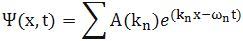
$\hat{E} \Psi = i\hbar\dfrac{\partial}{\partial t}\Psi = E\Psi$ Now if we plug that in the equation above, we get our time-dependent Schrödinger equation:

$i \hbar \frac{\partial}{\partial t}\Psi = \hat H \Psi$

OK. You probably did not understand one iota of this but, even then, you will object that this does not resemble the equation I wrote at the very beginning: i(∂u/∂t) = (-1/2)∇²u.

You’re right, but we only need one more step for that. If we leave out potential energy (so we assume a particle moving in free space), then the Hamiltonian can be written as:

$\hat{H} = -\frac{\hbar^2}{2m}\nabla^2$

You’ll ask me how this is done but I will be short on that: the relationship between energy and momentum is being used here (and so that’s where the 2m factor in the denominator comes from). However, I won’t say more about it because this post would become way too lengthy if I would include each and every derivation and, remember, I just want to get to the result because the derivations here are not the point: I want you to understand the functional form of the wave equation only. So, using the above identity and, OK, let’s be somewhat more complete and include potential energy once again, we can write the time-dependent wave equation as:

$i\hbar\frac{\partial}{\partial t}\Psi(\mathbf{r},t) = -\frac{\hbar^2}{2m}\nabla^2\Psi(\mathbf{r},t) + V(\mathbf{r},t)\Psi(\mathbf{r},t)$

Now, how is the equation above related to i(∂u/∂t) = (-1/2)∇²u? It’s a very simplified version of it: potential energy is, once again, assumed to be not relevant (so we’re talking a free particle again, with no external forces acting on it) but the real simplification is that we give m and ħ the value 1, so m = ħ = 1. Why?

Well… My initial idea was to do something similar as I did above and, hence, actually use a specific example with an actual functional form, just like we did for that the real-valued u(x, t) function. However, when I look at how long this post has become already, I realize I should not do that. In fact, I would just copy an example from somewhere else – probably Wikipedia once again, if only because their examples are usually nicely illustrated with graphs (and often animated graphs). So let me just refer you here to the other example given in the Wikipedia article on wave packets: that example uses that simplified i(∂u/∂t) = (-1/2)∇²u equation indeed. It actually uses the same initial condition:

However, because the wave equation is different, the wave packet behaves differently. It’s a so-called dispersive wave packet: it delocalizes. Its width increases over time and so, after a while, it just vanishes because it diffuses all over space. So there’s a solution to the wave equation, given this initial condition, but it’s just not stable – as a description of some particle that is (from a mathematical point of view – or even a physical point of view – there is no issue).

In any case, this probably all sounds like Chinese – or Greek if you understand Chinese :-). I actually haven’t worked with these Hermitian operators yet, and so it’s pretty shaky territory for me myself. However, I felt like I had picked up enough math and physics on this long and winding Road to Reality (I don’t think I am even halfway) to give it a try. I hope I succeeded in passing the message, which I’ll summarize as follows:

Schrödinger’s equation is just like any other differential equation used in physics, in the sense that it represents a system subject to constraints, such as the relationship between energy and momentum.
It will have many general solutions. In other words, the wave function – which describes a probability amplitude as a function in space and time – will have many general solutions, and a specific solution will depend on the initial conditions.
The solution(s) can represent stationary states, but not necessary so: a wave (or a wave packet) can be non-dispersive or dispersive. However, when we plug the wave function into the wave equation, it will satisfy that equation.

That’s neither spectacular nor difficult, is it? But, perhaps, it helps you to ‘understand’ wave equations, including the Schrödinger equation. But what is understanding? Dirac once famously said: “I consider that I understand an equation when I can predict the properties of its solutions, without actually solving it.”

Hmm… I am not quite there yet, but I am sure some more practice with it will help. 🙂

Post scriptum: On Maxwell’s equations

First, we should say something more about these two other operators which I introduced above: the divergence and the curl. First on the divergence.

The divergence of a field vector E (or B) at some point r represents the so-called flux of E, i.e. the ‘flow’ of E per unit volume. So flux and divergence both deal with the ‘flow’ of electric field lines away from (positive) charges. [The ‘away from’ is from positive charges indeed – as per the convention: Maxwell himself used the term ‘convergence’ to describe flow towards negative charges, but so his ‘convention’ did not survive. Too bad, because I think convergence would be much easier to remember.]

So if we write that ∇•E = ρ/ε₀, then it means that we have some constant flux of E because of some (fixed) distribution of charges.

Now, we already mentioned that equation (2) in Maxwell’s set meant that there is no such thing as a ‘magnetic’ charge: indeed, ∇•B = 0 means there is no magnetic flux. But, of course, magnetic fields do exist, don’t they? They do. A current in a wire, for example, i.e. a bunch of steadily moving electric charges, will induce a magnetic field according to Ampère’s law, which is part of equation (4) in Maxwell’s set: c²∇×B = j/ε₀, with j representing the current density and ε₀ the electric constant.

Now, at this point, we have this curl: ∇×B. Just like divergence (or convergence as Maxwell called it – but then with the sign reversed), curl also means something in physics: it’s the amount of ‘rotation’, or ‘circulation’ as Feynman calls it, around some loop.

So, to summarize the above, we have (1) flux (divergence) and (2) circulation (curl) and, of course, the two must be related. And, while we do not have any magnetic charges and, hence, no flux for B, the current in that wire will cause some circulation of B, and so we do have a magnetic field. However, that magnetic field will be static, i.e. it will not change. Hence, the time derivative ∂B/∂t will be zero and, hence, from equation (2) we get that ∇×E = 0, so our electric field will be static too. The time derivative ∂E/∂t which appears in equation (4) also disappears and we just have c²∇×B = j/ε₀. This situation – of a constant magnetic and electric field – is described as electrostatics and magnetostatics respectively. It implies a neat separation of the four equations, and it makes magnetism and electricity appear as distinct phenomena. Indeed, as long as charges and currents are static, we have:

[I] Electrostatics: (1) ∇•E = ρ/ε₀and (2) ∇×E = 0

[II] Magnetostatics: (3) c²∇×B = j/ε₀and (4) ∇•B = 0

The first two equations describe a vector field with zero curl and a given divergence (i.e. the electric field) while the third and fourth equations second describe a seemingly separate vector field with a given curl but zero divergence. Now, I am not writing this post scriptum to reproduce Feynman’s Lectures on Electromagnetism, and so I won’t say much more about this. I just want to note two points:

1. The first point to note is that factor c²in the c²∇×B = j/ε₀equation. That’s something which you don’t have in the ∇•E = ρ/ε₀equation. Of course, you’ll say: So what? Well… It’s weird. And if you bring it to the other side of the equation, it becomes clear that you need an awful lot of current for a tiny little bit of magnetic circulation (because you’re dividing by c² , so that’s a factor 9 with 16 zeroes after it (9×10¹⁶): an awfully big number in other words). Truth be said, it reveals something very deep. Hmm? Take a wild guess. […] Relativity perhaps? Well… Yes!

It’s obvious that we buried v somewhere in this equation, the velocity of the moving charges. But then it’s part of j of course: the rate at which charge flows through a unit area per second. But – Hey! – velocity as compared to what? What’s the frame of reference? The frame of reference is us obviously or – somewhat less subjective – the stationary charges determining the electric field according to equation (1) in the set above: ∇•E = ρ/ε₀. But so here we can ask the same question: stationary in what reference frame? As compared to the moving charges? Hmm… But so how does it work with relativity? I won’t copy Feynman’s 13th Lecture here, but so, in that lecture, he analyzes what happens to the electric and magnetic force when we look at the scene from another coordinate system – let’s say one that moves parallel to the wire at the same speed as the moving electrons, so – because of our new reference frame – the ‘moving electrons’ now appear to have no speed at all but, of course, our stationary charges will now seem to move.

What Feynman finds – and his calculations are very easy and straightforward – is that, while we will obviously insert different input values into Maxwell’s set of equations and, hence, get different values for the E and B fields, the actual physical effect – i.e. the final Lorentz force on a (charged) particle – will be the same. To be very specific, in a coordinate system at rest with respect to the wire (so we see charges move in the wire), we find a ‘magnetic’ force indeed, but in a coordinate system moving at the same speed of those charges, we will find an ‘electric’ force only. And from yet another reference frame, we will find a mixture of E and B fields. However, the physical result is the same: there is only one combined force in the end – the Lorentz force F = q(E + v×B) – and it’s always the same, regardless of the reference frame (inertial or moving at whatever speed – relativistic (i.e. close to c) or not).

In other words, Maxwell’s description of electromagnetism is invariant or, to say exactly the same in yet other words, electricity and magnetism taken together are consistent with relativity: they are part of one physical phenomenon: the electromagnetic interaction between (charged) particles. So electric and magnetic fields appear in different ‘mixtures’ if we change our frame of reference, and so that’s why magnetism is often described as a ‘relativistic’ effect – although that’s not very accurate. However, it does explain that c²factor in the equation for the curl of B. [How exactly? Well… If you’re smart enough to ask that kind of question, you will be smart enough to find the derivation on the Web. :-)]

Note: Don’t think we’re talking astronomical speeds here when comparing the two reference frames. It would also work for astronomical speeds but, in this case, we are talking the speed of the electrons moving through a wire. Now, the so-called drift velocity of electrons – which is the one we have to use here – in a copper wire of radius 1 mm carrying a steady current of 3 Amps is only about 1 m per hour! So the relativistic effect is tiny – but still measurable !

2. The second thing I want to note is that Maxwell’s set of equations with non-zero time derivatives for E and B clearly show that it’s changing electric and magnetic fields that sort of create each other, and it’s this that’s behind electromagnetic waves moving through space without losing energy. They just travel on and on. The math behind this is beautiful (and the animations in the related Wikipedia articles are equally beautiful – and probably easier to understand than the equations), but that’s stuff for another post. As the electric field changes, it induces a magnetic field, which then induces a new electric field, etc., allowing the wave to propagate itself through space. I should also note here that the energy is in the field and so, when electromagnetic waves, such as light, or radiowaves, travel through space, they carry their energy with them.

Let me be fully complete here, and note that there’s energy in electrostatic fields as well, and the formula for it is remarkably beautiful. The total (electrostatic) energy U in an electrostatic field generated by charges located within some finite distance is equal to:

This equation introduces the electrostatic potential. This is a scalar field Φ from which we can derive the electric field vector just by applying the gradient operator. In fact, all curl-free fields (such as the electric field in this case) can be written as the gradient of some scalar field. That’s a universal truth. See how beautiful math is? 🙂

End of the Road to Reality?

Pre-scriptum (dated 26 June 2020): This post did not suffer from the DMCA take-down of some material. It is, therefore, still quite readable—even if my views on these matters have evolved quite a bit as part of my realist interpretation of QM. I now think the idea of force-carrying particles (bosons) is quite medieval. Moreover, I think the Higgs particle and other bosons (except for the photon and the neutrino) are just short-lived transients or resonances. Disequilibrium states, in other words. One should not refer to them as particles.

Original post:

Or the end of theoretical physics?

In my previous post, I mentioned the Goliath of science and engineering: the Large Hadron Collider (LHC), built by the European Organization for Nuclear Research (CERN) under the Franco-Swiss border near Geneva. I actually started uploading some pictures, but then I realized I should write a separate post about it. So here we go.

The first image (see below) shows the LHC tunnel, while the other shows (a part of) one of the two large general-purpose particle detectors that are part of this Large Hadron Collider. A detector is the thing that’s used to look at those collisions. This is actually the smallest of the two general-purpose detectors: it’s the so-called CMS detector (the other one is the ATLAS detector), and it’s ‘only’ 21.6 meter long and 15 meter in diameter – and it weighs about 12,500 tons. But so it did detect a Higgs particle – just like the ATLAS detector. [That’s actually not 100% sure but it was sure enough for the Nobel Prize committee – so I guess that should be good enough for us common mortals :-)]

The picture above shows one of these collisions in the CMS detector. It’s not the one with the trace of the Higgs particle though. In fact, I have not found any image that actually shows the Higgs particle: the closest thing to such image are some impressionistic images on the ATLAS site. See http://atlas.ch/news/2013/higgs-into-fermions.html

In case you wonder what’s being scattered here… Well… All kinds of things – but so the original collision is usually between protons (so these are hydrogen ions: H⁺nuclei), although the LHC can produce other nucleon beams as well (collectively referred to as hadrons). These protons have energy levels of 4 TeV (tera-electronVolt: 1 TeV = 1000 GeV = 1 trillion eV = 1×10¹² eV).

Now, let’s think about scale once again. Remember (from that same previous post) that we calculated a wavelength of 0.33 nanometer (1 nm = 1×10^–9 m, so that’s a billionth of a meter) for an electron. Well, this LHC is actually exploring the sub-femtometer (fm) frontier. One femtometer (fm) is 1×10^–15 m so that’s another million times smaller. Yes: so we are talking a millionth of a billionth of a meter. The size of a proton is an estimated 1.7 femtometer indeed and, as you surely know, a proton is a point-like thing occupying a very tiny space, so it’s not like an electron ‘cloud’ swirling around: it’s much smaller. In fact, quarks – three of them make up a proton (or a neutron) – are usually thought of as being just a little bit less than half that size – so that’s about 0.7 fm.

It may also help you to use the value I mentioned for high-energy electrons when I was discussing the LEP (the Large Electron-Positron Collider, which preceded the LHC) – so that was 104.5 GeV – and calculate the associated de Broglie wavelength using E = hf and λ = v/f. The velocity v is close to c and, hence, if we plug everything in, we get a value close to 1.2×10^–15 m indeed, so that’s the femtometer scale indeed. [If you don’t want to calculate anything, then just note we’re going from eV to giga-eV energy levels here, and so our wavelength decreases accordingly: one billion times smaller. Also remember (from the previous posts) that we calculated a wavelength of 0.33×10^–6 m and an associated energy level of 70 eV for a slow-moving electron – i.e. one going at 2200 km per second ‘only’, i.e. less than 1% of the speed of light.] Also note that, at these energy levels, it doesn’t matter whether or not we include the rest mass of the electron: 0.511 MeV is nothing as compared to the GeV realm. In short, we are talking very very tiny stuff here.

But so that’s the LEP scale. I wrote that the LHC is probing things at the sub-femtometer scale. So how much sub-something is that? Well… Quite a lot: the LHC is looking at stuff at a scale that’s more than a thousand times smaller. Indeed, if collision experiments in the giga-electronvolt (GeV) energy range correspond to probing stuff at the femtometer scale, then tera-electronvolt (TeV) energy levels correspond to probing stuff that’s, once again, another thousand times smaller, so we’re looking at distances of less than a thousandth of a millionth of a billionth of a meter. Now, you can try to ‘imagine’ that, but you can’t really.

So what do we actually ‘see’ then? Well… Nothing much one could say: all we can ‘see’ are traces of point-like ‘things’ being scattered, which then disintegrate or just vanish from the scene – as shown in the image above. In fact, as mentioned above, we do not even have such clear-cut ‘trace’ of a Higgs particle: we’ve got a ‘kinda signal’ only. So that’s it? Yes. But then these images are beautiful, aren’t they? If only to remind ourselves that particle physics is about more than just a bunch of formulas. It’s about… Well… The essence of reality: its intrinsic nature so to say. So… Well…

Let me be skeptical. So we know all of that now, don’t we? The so-called Standard Model has been confirmed by experiment. We now know how Nature works, don’t we? We observe light (or, to be precise, radiation: most notably that cosmic background radiation that reaches us from everywhere) that originated nearly 14 billion years ago (to be precise: 380,000 years after the Big Bang – but what’s 380,000 years on this scale?) and so we can ‘see’ things that are 14 billion light-years away. In fact, things that were 14 billion light-years away: indeed, because of the expansion of the universe, they are further away now and so that’s why the so-called observable universe is actually larger. So we can ‘see’ everything we need to ‘see’ at the cosmic distance scale and now we can also ‘see’ all of the particles that make up matter, i.e. quarks and electrons mainly (we also have some other so-called leptons, like neutrinos and muons), and also all of the particles that make up anti-matter of course (i.e. antiquarks, positrons etcetera). As importantly – or even more – we can also ‘see’ all of the ‘particles’ carrying the forces governing the interactions between the ‘matter particles’ – which are collectively referred to as fermions, as opposed to the ‘force carrying’ particles, which are collectively referred to as bosons (see my previous post on Bose and Fermi). Let me quickly list them – just to make sure we’re on the same page:

Photons for the electromagnetic force.
Gluons for the so-called strong force, which explains why positively charged protons ‘stick’ together in nuclei – in spite of their electric charge, which should push them away from each other. [You might think it’s the neutrons that ‘glue’ them together but so, no, it’s the gluons.]
W⁺, W^–, and Z bosons for the so-called ‘weak’ interactions (aka as Fermi’s interaction), which explain how one type of quark can change into another, thereby explaining phenomena such as beta decay. [For example, carbon-14 will – through beta decay – spontaneously decay into nitrogen-14. Indeed, carbon-12 is the stable isotope, while carbon-14 has a life-time of 5,730 ± 40 years ‘only’ 🙂 and, hence, measuring how much carbon-14 is left in some organic substance allows us to date it (that’s what (radio)carbon-dating is about). As for the name, a beta particle can refer to an electron or a positron, so we can have β^– decay (e.g. the above-mentioned carbon-14 decay) as well as β⁺decay (e.g. magnesium-23 into sodium-23). There’s also alpha and gamma decay but that involves different things. In any case… Let me end this digression within the digression.]
Finally, the existence of the Higgs particle – and, hence, of the associated Higgs field – has been predicted since 1964 already, but so it was only experimentally confirmed (i.e. we saw it, in the LHC) last year, so Peter Higgs – and a few others of course – got their well-deserved Nobel prize only 50 years later. The Higgs field gives fermions, and also the W⁺, W^–, and Z bosons, mass (but not photons and gluons, and so that’s why the weak force has such short range – as compared to the electromagnetic and strong forces).

So there we are. We know it all. Sort of. Of course, there are many questions left – so it is said. For example, the Higgs particle does actually not explain the gravitational force, so it’s not the (theoretical) graviton, and so we do not have a quantum field theory for the gravitational force. [Just Google it and you’ll see why: there’s theoretical as well as practical (experimental) reasons for that.] Secondly, while we do have a quantum field theory for all of the forces (or ‘interactions’ as physicists prefer to call them), there are a lot of constants in them (much more than just that Planck constant I introduced in my posts!) that seem to be ‘unrelated and arbitrary.’ I am obviously just quoting Wikipedia here – but it’s true.

Just look at it: three ‘generations’ of matter with various strange properties, four force fields (and some ‘gauge theory’ to provide some uniformity), bosons that have mass (the W⁺, W^–, and Z bosons, and then the Higgs particle itself) but then photons and gluons don’t… It just doesn’t look good, and then Feynman himself wrote, just a few years before his death (QED, 1985, p. 128), that the math behind calculating some of these constants (the coupling constant j for instance, or the rest mass n of an electron), which he actually invented (it makes use of a mathematical approximation method called perturbation theory) and for which he got a Nobel Prize, is a “dippy process” and that “having to resort to such hocus-pocus has prevented us from proving that the theory of quantum electrodynamics is mathematically self-consistent“. He adds: “It’s surprising that the theory still hasn’t been proved self-consistent one way or the other by now; I suspect that renormalization [“the shell game that we play to find n and j” as he calls it] is not mathematically legitimate.” And so he writes this about quantum electrodynamics, not about “the rest of physics” (and so that’s quantum chromodynamics (QCD) – the theory of the strong interactions – and quantum flavordynamics (QFD) – the theory of weak interactions) which, he adds, “has not been checked anywhere near as well as electrodynamics.”

Waw ! That’s a pretty damning statement, isn’t it? In short, all of the celebrations around the experimental confirmation of the Higgs particle cannot hide the fact that it all looks a bit messy. There are other questions as well – most of which I don’t understand so I won’t mention them. To make a long story short, physicists and mathematicians alike seem to think there must be some ‘more fundamental’ theory behind. But – Hey! – you can’t have it all, can you? And, of course, all these theoretical physicists and mathematicians out there do need to justify their academic budget, don’t they? And so all that talk about a Grand Unification Theory (GUT) is probably just what is it: talk. Isn’t it? Maybe.

The key question is probably easy to formulate: what’s beyond this scale of a thousandth of a proton diameter (0.001×10^–15m) – a thousandth of a millionth of a billionth of a meter that is. Well… Let’s first note that this so-called ‘beyond’ is a ‘universe’ which mankind (or let’s just say ‘we’) will never see. Never ever. Why? Because there is no way to go substantially beyond the 4 TeV energy levels that were reached last year – at great cost – in the world’s largest particle collider (the LHC). Indeed, the LHC is widely regarded not only as “the most complex and ambitious scientiﬁc project ever accomplished by humanity” (I am quoting a CERN scientist here) but – with a cost of more than 7.5 billion Euro – also as one of the most expensive ones. Indeed, taking into account inflation and all that, it was like the Manhattan project indeed (although scientists loathe that comparison). So we should not have any illusions: there will be no new super-duper LHC any time soon, and surely not during our lifetime: the current LHC is the super-duper thing!

Indeed, when I write ‘substantially‘ above, I really mean substantially. Just to put things in perspective: the LHC is currently being upgraded to produce 7 TeV beams (it was shut down for this upgrade, and it should come back on stream in 2015). That sounds like an awful lot (from 4 to 7 is +75%), and it is: it amounts to packing the kinetic energy of seven flying mosquitos (instead of four previously :-)) into each and every particle that makes up the beam. But that’s not substantial, in the sense that it is very much below the so-called GUT energy scale, which is the energy level above which, it is believed (by all those GUT theorists at least), the electromagnetic force, the weak force and the strong force will all be part and parcel of one and the same unified force. Don’t ask me why (I’ll know when I finished reading Penrose, I hope) but that’s what it is (if I should believe what I am reading currently that is). In any case, the thing to remember is that the GUT energy levels are in the 10¹⁶ GeV range, so that’s – sorry for all these numbers – a trillion TeV. That amounts to pumping more than 160,000 Joule in each of those tiny point-like particles that make up our beam. So… No. Don’t even try to dream about it. It won’t happen. That’s science fiction – with the emphasis on fiction. [Also don’t dream about a trillion flying mosquitos packed into one proton-sized super-mosquito either. :-)]

So what?

Well… I don’t know. Physicists refer to the zone beyond the above-mentioned scale (so things smaller than 0.001×10^–15m) as the Great Desert. That’s a very appropriate name I think – for more than one reason. And so it’s this ‘desert’ that Roger Penrose is actually trying to explore in his ‘Road to Reality’. As for me, well… I must admit I have great trouble following Penrose on this road. I’ve actually started to doubt that Penrose’s Road leads to Reality. Maybe it takes us away from it. Huh? Well… I mean… Perhaps the road just stops at that 0.001×10^–15m frontier?

In fact, that’s a view which one of the early physicists specialized in high-energy physics, Raoul Gatto, referred to as the zeroth scenario. I am actually not quoting Gatto here, but another theoretical physicist: Gerard ‘t Hooft, another Nobel prize winner (you may know him better because he’s a rather fervent Mars One supporter, but so here I am referring to his popular 1996 book In Search of the Ultimate Building Blocks). In any case, Gatto, and most other physicists, including ‘T Hooft (despite the fact ‘T Hooft got his Nobel prize for his contribution to gauge theory – which, together with Feynman’s application of perturbation theory to QED, is actually the backbone of the Standard Model) firmly reject this zeroth scenario. ‘T Hooft himself thinks superstring theory (i.e. supersymmetric string theory – which has now been folded into M-theory or – back to the original term – just string theory – the terminology is quite confusing) holds the key to exploring this desert.

But who knows? In fact, we can’t – because of the above-mentioned practical problem of experimental confirmation. So I am likely to stay on this side of the frontier for quite a while – if only because there’s still so much to see here and, of course, also because I am just at the beginning of this road. 🙂 And then I also realize I’ll need to understand gauge theory and all that to continue on this road – which is likely to take me another six months or so (if not more) and then, only then, I might try to look at those little strings, even if we’ll never see them because… Well… Their theoretical diameter is the so-called Planck length. So what? Well… That’s equal to 1.6×10⁻³⁵m. So what? Well… Nothing. It’s just that 1.6×10⁻³⁵m is 1/10 000 000 000 000 000 of that sub-femtometer scale. I don’t even want to write this in trillionths of trillionths of trillionths etcetera because I feel that’s just not making any sense. And perhaps it doesn’t. One thing is for sure: that ‘desert’ that GUT theorists want us to cross is not just ‘Great’: it’s ENORMOUS!

Richard Feynman – another Nobel Prize scientist whom I obviously respect a lot – surely thought trying to cross a desert like that amounts to certain death. Indeed, he’s supposed to have said the following about string theorists, about a year or two before he died (way too young): “I don’t like that they’re not calculating anything. I don’t like that they don’t check their ideas. I don’t like that for anything that disagrees with an experiment, they cook up an explanation–a fix-up to say, “Well, it might be true.” For example, the theory requires ten dimensions. Well, maybe there’s a way of wrapping up six of the dimensions. Yes, that’s all possible mathematically, but why not seven? When they write their equation, the equation should decide how many of these things get wrapped up, not the desire to agree with experiment. In other words, there’s no reason whatsoever in superstring theory that it isn’t eight out of the ten dimensions that get wrapped up and that the result is only two dimensions, which would be completely in disagreement with experience. So the fact that it might disagree with experience is very tenuous, it doesn’t produce anything; it has to be excused most of the time. It doesn’t look right.”

Hmm… Feynman and ‘T Hooft… Two giants in science. Two Nobel Prize winners – and for stuff that truly revolutionized physics. The amazing thing is that those two giants – who are clearly at loggerheads on this one – actually worked closely together on a number of other topics – most notably on the so-called Feynman-‘T Hooft gauge, which – as far as I understand – is the one that is most widely used in quantum field calculations. But I’ll leave it at that here – and I’ll just make a mental note of the terminology here. The Great Desert… Probably an appropriate term. ‘T Hooft says that most physicists think that desert is full of tiny flowers. I am not so sure – but then I am not half as smart as ‘T Hooft. Much less actually. So I’ll just see where the road I am currently following leads me. With Feynman’s warning in mind, I should probably expect the road condition to deteriorate quickly.

Post scriptum: You will not be surprised to hear that there’s a word for 1×10^–18m: it’s called an attometer (with two t’s, and abbreviated as am). And beyond that we have zeptometer (1 zm = 1×10^–21m) and yoctometer (1 ym = 1×10^–23m). In fact, these measures actually represent something: 20 yoctometer is the estimated radius of a 1 MeV neutrino – or, to be precise, its the radius of the cross section, which is “the effective area that governs the probability of some scattering or absorption event.” But so then there are no words anymore. The next measure is the Planck length: 1.62 × 10⁻³⁵ m – but so that’s a trillion (10¹²) times smaller than a yoctometer. Unimaginable, isn’t it? Literally.

Note: A 1 MeV neutrino? Well… Yes. The estimated rest mass of an (electron) neutrino is tiny: at least 50,000 times smaller than the mass of the electron and, therefore, neutrinos are often assumed to be massless, for all practical purposes that is. However, just like the massless photon, they can carry high energy. High-energy gamma ray photons, for example, are also associated with MeV energy levels. Neutrinos are one of the many particles produced in high-energy particle collisions in particle accelerators, but they are present everywhere: they’re produced by stars (which, as you know, are nuclear fusion reactors). In fact, most neutrinos passing through Earth are produced by our Sun. The largest neutrino detector on Earth is called IceCube. It sits on the South Pole – or under it, as it’s suspended under the Antarctic ice, and it regularly captures high-energy neutrinos in the range of 1 to 10 TeV. Last year (in November 2013), it captured two with energy levels around 1000 TeV – so that’s the peta-electronvolt level (1 PeV = 1×10¹⁵eV). If you think that’s amazing, it is. But also remember that 1 eV is 1.6×10⁻¹⁹Joule, so it’s ‘only’ a ten-thousandth of a Joule. In other words, you would need at least ten thousand of them to briefly light up an LED. The PeV pair was dubbed Bert and Ernie and the illustration below (from IceCube’s website) conveys how the detectors sort of lit up when they passed. It was obviously a pretty clear ‘signal’ – but so the illustration also makes it clear that we don’t really ‘see’ at such small scale: we just know ‘something’ happened.

The Uncertainty Principle re-visited: Fourier transforms and conjugate variables

Pre-scriptum (dated 26 June 2020): This post did not suffer from the DMCA take-down of some material. It is, therefore, still quite readable—even if my views on the nature of the Uncertainty Principle have evolved quite a bit as part of my realist interpretation of QM.

Original post:

In previous posts, I presented a time-independent wave function for a particle (or wavicle as we should call it – but so that’s not the convention in physics) – let’s say an electron – traveling through space without any external forces (or force fields) acting upon it. So it’s just going in some random direction with some random velocity v and, hence, its momentum is p = mv. Let me be specific – so I’ll work with some numbers here – because I want to introduce some issues related to units for measurement.

So the momentum of this electron is the product of its mass m (about 9.1×10⁻²⁸ grams) with its velocity v (typically something in the range around 2,200 km/s, which is fast but not even close to the speed of light – and, hence, we don’t need to worry about relativistic effects on its mass here). Hence, the momentum p of this electron would be some 20×10⁻²⁵ kg·m/s. Huh? Kg·m/s?Well… Yes, kg·m/s or N·s are the usual measures of momentum in classical mechanics: its dimension is [mass][length]/[time] indeed. However, you know that, in atomic physics, we don’t want to work with these enormous units (because we then always have to add these ×10⁻²⁸ and ×10⁻²⁵ factors and so that’s a bit of a nuisance indeed). So the momentum p will usually be measured in eV/c, with c representing what it usually represents, i.e. the speed of light. Huh? What’s this strange unit? Electronvolts divided by c? Well… We know that eV is an appropriate unit for measuring energy in atomic physics: we can express eV in Joule and vice versa: 1 eV = 1.6×10⁻¹⁹Joule, so that’s OK – except for the fact that this Joule is a monstrously large unit at the atomic scale indeed, and so that’s why we prefer electronvolt. But the Joule is a shorthand unit for kg·m²/s², which is the measure for energy expressed in SI units, so there we are: while the SI dimension for energy is actually [mass][length]²/[time]², using electronvolts (eV) is fine. Now, just divide the SI dimension for energy, i.e. [mass][length]²/[time]², by the SI dimension for velocity, i.e. [length]/[time]: we get something expressed in [mass][length]/[time]. So that’s the SI dimension for momentum indeed! In other words, dividing some quantity expressed in some measure for energy (be it Joules or electronvolts or erg or calories or coulomb-volts or BTUs or whatever – there’s quite a lot of ways to measure energy indeed!) by the speed of light (c) will result in some quantity with the right dimensions indeed. So don’t worry about it. Now, 1 eV/c is equivalent to 5.344×10⁻²⁸ kg·m/s, so the momentum of this electron will be 3.75 eV/c.

Let’s go back to the main story now. Just note that the momentum of this electron that we are looking at is a very tiny amount – as we would expect of course.

Time-independent means that we keep the time variable (t) in the wave function Ψ(x, t) fixed and so we only look at how Ψ(x, t) varies in space, with x as the (real) space variable representing position. So we have a simplified wave function Ψ(x) here: we can always put the time variable back in when we’re finished with the analysis. By now, it should also be clear that we should distinguish between real-valued wave functions and complex-valued wave functions. Real-valued wave functions represent what Feynman calls “real waves”, like a sound wave, or an oscillating electromagnetic field. Complex-valued wave functions describe probability amplitudes. They are… Well… Feynman actually stops short of saying that they are not real. So what are they?

They are, first and foremost complex numbers, so they have a real and a so-called imaginary part (z = a + ib or, if we use polar coordinates, re^θ= cosθ + isinθ). Now, you may think – and you’re probably right to some extent – that the distinction between ‘real’ waves and ‘complex’ waves is, perhaps, less of a dichotomy than popular writers – like me 🙂 – suggest. When describing electromagnetic waves, for example, we need to keep track of both the electric field vector E as well as the magnetic field vector B (both are obviously related through Maxwell’s equations). So we have two components as well, so to say, and each of these components has three dimensions in space, and we’ll use the same mathematical tools to describe them (so we will also represent them using complex numbers). That being said, these probability amplitudes, usually denoted by Ψ(x), describe something very different. What exactly? Well… By now, it should be clear that that is actually hard to explain: the best thing we can do is to work with them, so they start feeling familiar. The main thing to remember is that we need to square their modulus (or magnitude or absolute value if you find these terms more comprehensible) to get a probability (P). For example, the expression below gives the probability of finding a particle – our electron for example – in in the (space) interval [a, b]:

Of course, we should not be talking intervals but three-dimensional regions in space. However, we’ll keep it simple: just remember that the analysis should be extended to three (space) dimensions (and, of course, include the time dimension as well) when we’re finished (to do that, we’d use so-called four-vectors – another wonderful mathematical invention).

Now, we also used a simple functional form for this wave function, as an example: Ψ(x) could be proportional, we said, to some idealized function e^ikx. So we can write: Ψ(x) ∝ e^ikx (∝ is the standard symbol expressing proportionality). In this function, we have a wave number k, which is like the frequency in space of the wave (but then measured in radians because the phase of the wave function has to be expressed in radians). In fact, we actually wrote Ψ(x, t) = (1/x)e^{i(kx – ωt)}(so the magnitude of this amplitude decreases with distance) but, again, let’s keep it simple for the moment: even with this very simple function e^ikx , things will become complex enough.

We also introduced the de Broglie relation, which gives this wave number k as a function of the momentum p of the particle: k = p/ħ, with ħ the (reduced) Planck constant, i.e. a very tiny number in the neighborhood of 6.582 ×10⁻¹⁶ eV·s. So, using the numbers above, we’d have a value for k equal to 3.75 eV/c divided by 6.582 ×10⁻¹⁶ eV·s. So that’s 0.57×10¹⁶ (radians) per… Hey, how do we do it with the units here? We get an incredibly huge number here (57 with 14 zeroes after it) per second? We should get some number per meter because k is expressed in radians per unit distance, right? Right. We forgot c. We are actually measuring distance here, but in light-seconds instead of meter: k is 0.57×10¹⁶/c·s. Indeed, a light-second is the distance traveled by light in one second, so that’s c·s, and if we want k expressed in radians per meter, then we need to divide this huge number 0.57×10¹⁶ (in rad) by 2.998×10⁸( in (m/s)·s) and so then we get a much more reasonable value for k, and with the right dimension too: to be precise, k is about 19×10⁶ rad/m in this case. That’s still huge: it corresponds with a wavelength of 0.33 nanometer (1 nm = 10^-6 m) but that’s the correct order of magnitude indeed.

[In case you wonder what formula I am using to calculate the wavelength: it’s λ = 2π/k. Note that our electron’s wavelength is more than a thousand times shorter than the wavelength of (visible) light (we humans can see light with wavelengths ranging from 380 to 750 nm) but so that’s what gives the electron its particle-like character! If we would increase their velocity (e.g. by accelerating them in an accelerator, using electromagnetic fields to propel them to speeds closer to c and also to contain them in a beam), then we get hard beta rays. Hard beta rays are surely not as harmful as high-energy electromagnetic rays. X-rays and gamma rays consist of photons with wavelengths ranging from 1 to 100 picometer (1 pm = 10^–12m) – so that’s another factor of a thousand down – and thick lead shields are needed to stop them: they are the cause of cancer (Marie Curie’s cause of death), and the hard radiation of a nuclear blast will always end up killing more people than the immediate blast effect. In contrast, hard beta rays will cause skin damage (radiation burns) but they won’t go deeper than that.]

Let’s get back to our wave function Ψ(x) ∝ e^ikx. When we introduced it in our previous posts, we said it could not accurately describe a particle because this wave function (Ψ(x) = Ae^ikx) is associated with probabilities |Ψ(x)|² that are the same everywhere. Indeed, |Ψ(x)|² = |Ae^ikx|² = A². Apart from the fact that these probabilities would add up to infinity (so this mathematical shape is unacceptable anyway), it also implies that we cannot locate our electron somewhere in space. It’s everywhere and that’s the same as saying it’s actually nowhere. So, while we can use this wave function to explain and illustrate a lot of stuff (first and foremost the de Broglie relations), we actually need something different if we would want to describe anything real (which, in the end, is what physicists want to do, right?). We already said in our previous posts: real particles will actually be represented by a wave packet, or a wave train. A wave train can be analyzed as a composite wave consisting of a (potentially infinite) number of component waves. So we write:

Note that we do not have one unique wave number k or – what amounts to saying the same – one unique value p for the momentum: we have n values. So we’re introducing a spread in the wavelength here, as illustrated below:

In fact, the illustration above talks of a continuous distribution of wavelengths and so let’s take the continuum limit of the function above indeed and write what we should be writing:

Now that is an interesting formula. [Note that I didn’t care about normalization issues here, so it’s not quite what you’d see in a more rigorous treatment of the matter. I’ll correct that in the Post Scriptum.] Indeed, it shows how we can get the wave function Ψ(x) from some other function Φ(p). We actually encountered that function already, and we referred to it as the wave function in the momentum space. Indeed, Nature does not care much what we measure: whether it’s position (x) or momentum (p), Nature will not share her secrets with us and, hence, the best we can do – according to quantum mechanics – is to find some wave function associating some (complex) probability amplitude with each and every possible (real) value of x or p. What the equation above shows, then, is these wave functions come as a pair: if we have Φ(p), then we can calculate Ψ(x) – and vice versa. Indeed, the particular relation between Ψ(x) and Φ(p) as established above, makes Ψ(x) and Φ(p) a so-called Fourier transform pair, as we can transform Φ(p) into Ψ(x) using the above Fourier transform (that’s how that integral is called), and vice versa. More in general, a Fourier transform pair can be written as:

Instead of x and p, and Ψ(x) and Φ(p), we have x and y, and f(x) and g(y), in the formulas above, but so that does not make much of a difference when it comes to the interpretation: x and p (or x and y in the formulas above) are said to be conjugate variables. What it means really is that they are not independent. There are quite a few of such conjugate variables in quantum mechanics such as, for example: (1) time and energy (and time and frequency, of course, in light of the de Broglie relation between both), and (2) angular momentum and angular position (or orientation). There are other pairs too but these involve quantum-mechanical variables which I do not understand as yet and, hence, I won’t mention them here. [To be complete, I should also say something about that 1/2π factor, but so that’s just something that pops up when deriving the Fourier transform from the (discrete) Fourier series on which it is based. We can put it in front of either integral, or split that factor across both. Also note the minus sign in the exponent of the inverse transform.]

When you look at the equations above, you may think that f(x) and g(y) must be real-valued functions. Well… No. The Fourier transform can be used for both real-valued as well as complex-valued functions. However, at this point I’ll have to refer those who want to know each and every detail about these Fourier transforms to a course in complex analysis (such as Brown and Churchill’s Complex Variables and Applications (2004) for instance) or, else, to a proper course on real and complex Fourier transforms (they are used in signal processing – a very popular topic in engineering – and so there’s quite a few of those courses around).

The point to note in this post is that we can derive the Uncertainty Principle from the equations above. Indeed, the (complex-valued) functions Ψ(x) and Φ(p) describe (probability) amplitudes, but the (real-valued) functions |Ψ(x)|² and |Φ(p)|² describe probabilities or – to be fully correct – they are probability (density) functions. So it is pretty obvious that, if the functions Ψ(x) and Φ(p) are a Fourier transform pair, then |Ψ(x)|² and |Φ(p)|² must be related to. They are. The derivation is a bit lengthy (and, hence, I will not copy it from the Wikipedia article on the Uncertainty Principle) but one can indeed derive the so-called Kennard formulation of the Uncertainty Principle from the above Fourier transforms. This Kennard formulation does not use this rather vague Δx and Δp symbols but clearly states that the product of the standard deviation from the mean of these two probability density functions can never be smaller than ħ/2:

σ_xσ_p≥ ħ/2

To be sure: ħ/2 is a rather tiny value, as you should know by now, 🙂 but, so, well… There it is.

As said, it’s a bit lengthy but not that difficult to do that derivation. However, just for once, I think I should try to keep my post somewhat shorter than usual so, to conclude, I’ll just insert one more illustration here (yes, you’ve seen that one before), which should now be very easy to understand: if the wave function Ψ(x) is such that there’s relatively little uncertainty about the position x of our electron, then the uncertainty about its momentum will be huge (see the top graphs). Vice versa (see the bottom graphs), precise information (or a narrow range) on its momentum, implies that its position cannot be known.

Does all this math make it any easier to understand what’s going on? Well… Yes and no, I guess. But then, if even Feynman admits that he himself “does not understand it the way he would like to” (Feynman Lectures, Vol. III, 1-1), who am I? In fact, I should probably not even try to explain it, should I? 🙂

So the best we can do is try to familiarize ourselves with the language used, and so that’s math for all practical purposes. And, then, when everything is said and done, we should probably just contemplate Mario Livio’s question: Is God a mathematician? 🙂

Post scriptum:

I obviously cut corners above, and so you may wonder how that ħ factor can be related to σ_xand σ _pif it doesn’t appear in the wave functions. Truth be told, it does. Because of (i) the presence of ħ in the exponent in our e^i(p/ħ)x function, (ii) normalization issues (remember that probabilities (i.e. Ψ|(x)|² and |Φ(p)|²) have to add up to 1) and, last but not least, (iii) the 1/2π factor involved in Fourier transforms , Ψ(x) and Φ(p) have to be written as follows:

Note that we’ve also re-inserted the time variable here, so it’s pretty complete now. One more thing we could do is to substitute x for a proper three-dimensional space vector x or, better still, introduce four-vectors, which would allow us to also integrate relativistic effects (most notably the slowing of time with motion – as observed from the stationary reference frame) – which become important when, for instance, we’re looking at electrons being accelerated, which is the rule, rather than the exception, in experiments.

Remember (from a previous post) that we calculated that an electron traveling at its usual speed in orbit (2200 km/s, i.e. less than 1% of the speed of light) had an energy of about 70 eV? Well, the Large Electron-Positron Collider (LEP) did accelerate them to speeds close to light, thereby giving them energy levels topping 104.5 billion eV (or 104.5 GeV as it’s written) so they could hit each other with collision energies topping 209 GeV (they come from opposite directions so it’s two times 104.5 GeV). Now, 209 GeV is tiny when converted to everyday energy units: 209 GeV is 33×10^–9Joule only indeed – and so note the minus sign in the exponent here: we’re talking billionths of a Joule here. Just to put things into perspective: 1 Watt is the energy consumption of an LED (and 1 Watt is 1 Joule per second), so you’d need to combine the energy of billions of these fast-traveling electrons to power just one little LED lamp. But, of course, that’s not the right comparison: 104.5 GeV is more than 200,000 times the electron’s rest mass (0.511 MeV), so that means that – in practical terms – their mass (remember that mass is a measure for inertia) increased by the same factor (204,500 times to be precise). Just to give an idea of the effort that was needed to do this: CERN’s LEP collider was housed in a tunnel with a circumference of 27 km. Was? Yes. The tunnel is still there but it now houses the Large Hadron Collider (LHC) which, as you surely know, is the world’s largest and most powerful particle accelerator: its experiments confirmed the existence of the Higgs particle in 2013, thereby confirming the so-called Standard Model of particle physics. [But I’ll see a few things about that in my next post.]

Oh… And, finally, in case you’d wonder where we get the inequality sign in σ_xσ_p≥ ħ/2, that’s because – at some point in the derivation – one has to use the Cauchy-Schwarz inequality (aka as the triangle inequality): |z₁+ z₁| ≤ |z₁|+| z₁|. In fact, to be fully complete, the derivation uses the more general formulation of the Cauchy-Schwarz inequality, which also applies to functions as we interpret them as vectors in a function space. But I would end up copying the whole derivation here if I add any more to this – and I said I wouldn’t do that. 🙂 […]