One Equation, Too Many Jobs: Rethinking Schrödinger’s Equation and Wavefunction

I have just republished one of my long-standing papers on de Broglie’s matter-wave concept as a new, standalone publication, with its own DOI:

👉 De Broglie’s matter-wave concept and issues
https://www.researchgate.net/publication/399225854_De_Broglie’s_matter-wave_concept_and_issues
DOI: 10.13140/RG.2.2.30104.25605

The reason for republishing is not cosmetic. A new Annex was added on 31 December 2025 that fundamentally clarified — for me, at least — what Schrödinger’s equation is really doing, and just as importantly, what it is not doing.

This clarification came out of a long and at times uncomfortable dialogue with the most recent version of OpenAI’s GPT model (ChatGPT 5.2). Uncomfortable, because it initially destabilized a view I had held for years. Productive, because it forced a deeper structural distinction that I now believe is unavoidable. Let me explain.

The uncomfortable admission: I was wrong about the $\tfrac{1}{2}$ factor

For a long time, I was convinced that the factor $\tfrac{1}{2}$ factor in Schrödinger’s equation — especially in the hydrogen atom problem — must reflect some deeper pairing mechanism. At times, I even wondered whether the equation was implicitly modeling an electron pair (opposite spin), rather than a single electron.

That intuition was not random. It came from a broader realist programme in which I treat the electron as a structured object, with internal dynamics (zitterbewegung-like orbital motion), not as a point particle. If mass, energy, and phase all have internal structure, why should a simple quadratic kinetic term with a mysterious $\tfrac{1}{2}$ be fundamental?

The hard truth is this: that intuition was misplaced — but it was pointing in the right direction.

The mistake was not questioning the factor $\tfrac{1}{2}$ . The mistake was assuming Schrödinger’s equation was trying to describe everything at once.

The key insight: Schrödinger describes the envelope, not the engine

The decisive realization was structural:

Schrödinger’s wavefunction does not describe the electron’s internal dynamics.
It describes the translational envelope of phase coherence.

Once you see that, several things fall into place immediately:

The hydrogen “orbitals” are not literal orbits, and not internal electron motion.
They are standing-wave solutions of an envelope phase, constrained by a Coulomb potential.
The factor $\tfrac{1}{2}$ is not mysterious at all at this level: it is the natural coefficient that appears in effective, averaged, quadratic envelope dynamics.

In other words:
The $\tfrac{1}{2}$ factor belongs to the envelope layer, not to the internal structure of the electron.

My earlier “electron pair” idea tried to explain a structural feature by inventing new ontology. The correct move was simpler and more radical: separate the layers.

One symbol, too many jobs

Modern quantum mechanics makes a profound — and in my view costly — simplification:

It uses one symbol, ψ, to represent:

internal phase,
translational dynamics,
probability amplitudes,
and experimental observables.

That compression works operationally, but it hides structure.

What the new Annex makes explicit is that Nature almost certainly does not work that way. At minimum, we should distinguish:

Internal phase
Real, physical, associated with internal orbital motion and energy bookkeeping.
Envelope phase
Slow modulation across space, responsible for interference, diffraction, and spectra.
Observables
What experiments actually measure, which are sensitive mainly to envelope-level phase differences.

Once this distinction is made, long-standing confusions dissolve rather than multiply.

Why this does not contradict experiments

This is crucial.

Nothing in this reinterpretation invalidates:

electron diffraction,
hydrogen spectra,
interference experiments,
or the empirical success of standard quantum mechanics.

On the contrary: it explains why Schrödinger’s equation works so well — within its proper domain.

The equation is not wrong.
It is just over-interpreted.

A personal note on changing one’s mind

I’ll be honest: this line of reasoning initially felt destabilizing. It challenged a position I had defended for years. But that discomfort turned out to be a feature, not a bug.

Good theory-building does not preserve intuitions at all costs. It preserves structure, coherence, and explanatory power.

What emerged is a cleaner picture:

internal realism without metaphysics,
Schrödinger demoted from “ultimate truth” to “effective envelope theory”,
and a much clearer map of where different mathematical tools belong.

That, to me, is progress.

Where this opens doors

Once we accept that one wavefunction cannot represent all layers of Nature, new possibilities open up:

clearer interpretations of spin and the Dirac equation,
better realist models of lattice propagation,
a more honest treatment of “quantum mysteries” as category mistakes,
and perhaps new mathematical frameworks that respect internal structure from the start.

Those are not promises — just directions.

For now, I am satisfied that one long-standing conceptual knot has been untied.

And sometimes, that’s enough for a good year’s work. 🙂

Post Scriptum: On AI, Intellectual Sparring, and the Corridor

A final remark, somewhat orthogonal to physics.

The revision that led to this blog post and the accompanying paper did not emerge from a sudden insight, nor from a decisive experimental argument. It emerged from a long, occasionally uncomfortable dialogue with an AI system, in which neither side “won,” but both were forced to refine their assumptions.

At the start of that dialogue, the AI responded in a largely orthodox way, reproducing standard explanations for the factor $\tfrac{1}{2}$ in Schrödinger’s equation. I, in turn, defended a long-held intuition that this factor must point to internal structure or pairing. What followed was not persuasion, but sparring: resistance on both sides, followed by a gradual clarification of conceptual layers. The breakthrough came when it became clear that a single mathematical object — the wavefunction — was being asked to do too many jobs at once.

From that moment on, the conversation shifted from “who is right?” to “which layer are we talking about?” The result was not a victory for orthodoxy or for realism, but a structural separation: internal phase versus translational envelope, engine versus modulation. That separation resolved a tension that had existed for years in my own thinking.

I have explored this mode of human–AI interaction more systematically in a separate booklet on ResearchGate, where I describe such exchanges as occurring within a corridor: a space in which disagreement does not collapse into dominance or deference, but instead forces both sides toward finer distinctions and more mature reasoning.

This episode convinced me that the real intellectual value of AI does not lie in answers, but in sustained resistance without ego — and in the willingness of the human interlocutor to tolerate temporary destabilization without retreating into dogma. When that corridor holds, something genuinely new can emerge.

In that sense, this post is not only about Schrödinger’s equation. It is also about how thinking itself may evolve when humans and machines are allowed to reason together, rather than merely agree.

Readers interested in this kind of human–AI interaction beyond the present physics discussion may want to look at that separate booklet I published on ResearchGate (≈100 pages), in which I try to categorize different modes of AI–human intellectual interaction — from superficial compliance and authority projection to genuine sparring. In that text, exchanges like the one briefly alluded to above are described as a Type-D collapse: a situation in which both human and AI are forced to abandon premature explanatory closure, without either side “winning,” and where progress comes from structural re-layering rather than persuasion.

The booklet is intentionally exploratory and occasionally playful in tone, but it grew out of exactly this kind of experience: moments where resistance, rather than agreement, turns out to be the most productive form of collaboration.

Schrödinger’s equation in action

Pre-script (dated 26 June 2020): Our ideas have evolved into a full-blown realistic (or classical) interpretation of all things quantum-mechanical. So no use to read this. Read my recent papers instead. 🙂

Original post:

This post is about something I promised to write about aeons ago: how do we get those electron orbitals out of Schrödinger’s equation? So let me write it now – for the simplest of atoms: hydrogen. I’ll largely follow Richard Feynman’s exposé on it: this text just intends to walk you through it and provide some comments here and there.

Let me first remind you of what that famous Schrödinger’s equation actually represents. In its simplest form – i.e. not including any potential, so then it’s an equation that’s valid for free space only—no force fields!—it reduces to:

i·ħ∙∂ψ/∂t = –(1/2)∙(ħ²/m_eff)∙∇²ψ

Note the enigmatic concept of the efficient mass in it (m_eff), as well as the rather awkward 1/2 factor, which we may get rid of by re-defining it. We then write: m_eff^NEW = 2∙m_eff^OLD, and Schrödinger’s equation then simplifies to:

∂ψ/∂t + i∙(V/ħ)·ψ = i(ħ/m_eff)·∇²ψ
In free space (no potential): ∂ψ/∂t = i∙(ħ/m_eff)·∇²ψ

In case you wonder where the minus sign went, I just brought the imaginary unit to the other side. Remember 1/i = −i. 🙂

Now, in my post on quantum-mechanical operators, I drew your attention to the fact that this equation is structurally similar to the heat diffusion equation – or to any diffusion equation, really. Indeed, assuming the heat per unit volume (q) is proportional to the temperature (T) – which is the case when expressing T in degrees Kelvin (K), so we can write q as q = k·T – we can write the heat diffusion equation as:

Moreover, I noted the similarity is not only structural. There is more to it: both equations model energy flows. How exactly is something I wrote about in my e-publication on this, so let me refer you to that. Let’s jot down the complete equation once more:

∂ψ/∂t + i∙(V/ħ)·ψ = i(ħ/m_eff)·∇²ψ

In fact, it is rather surprising that Feynman drops the eff subscript almost immediately, so he just writes:

Let me first remind you that ψ is a function of position in space and time, so we write: ψ = ψ(x, y, z, t) = ψ(r, t), with (x, y, z) = r. And m, on the other side of the equation, is what it always was: the effective electron mass. Now, we talked about the subtleties involved before, so let’s not bother about the definition of the effective electron mass, or wonder where that factor 1/2 comes from here.

What about V? V is the potential energy of the electron: it depends on the distance (r) from the proton. We write: V = −e²/│r│ = −e²/r. Why the minus sign? Because we say the potential energy is zero at large distances (see my post on potential energy). Back to Schrödinger’s equation.

On the left-hand side, we have ħ, and its dimension is J·s (or N·m·s, if you want). So we multiply that with a time derivative and we get J, the unit of energy. On the right-hand side, we have Planck’s constant squared, the mass factor in the denominator, and the Laplacian operator – i.e. ∇²= ∇·∇, with ∇ = (∂/∂x, ∂/∂y, ∂/∂z) – operating on the wavefunction.

Let’s start with the latter. The Laplacian works just the same as for our heat diffusion equation: it gives us a flux density, i.e. something expressed per square meter (1/m²). The ħ²factor gives us J²·s². The mass factor makes everything come out alright, if we use the mass-equivalence relation, which says it’s OK to express the mass in J/(m/s)². [The mass of an electron is usually expressed as being equal to 0.5109989461(31) MeV/c². That unit uses the E = m·c²mass-equivalence formula. As for the eV, you know we can convert that into joule, which is a rather large unit—which is why we use the electronvolt as a measure of energy.] To make a long story short, we’re OK: (J²·s²)·[(m/s)²/J]·(1/m²) = J! Perfect. [As for the Vψ term, that’s obviously expressed in joule too.]

In short, Schrödinger’s equation expresses the energy conservation law too, and we may express it per square meter or per second or per cubic meter as well, if we’d wish: we can just multiply both sides by 1/m² or 1/s or 1/m³or by whatever dimension you want. Again, if you want more detail on the Schrödinger equation as an energy propagation mechanism, read the mentioned e-publication. So let’s get back to our equation, which, taking into account our formula for V, now looks like this:

Feynman then injects one of these enigmatic phrases—enigmatic for novices like us, at least!

“We want to look for definite energy states, so we try to find solutions which have the form: ψ (r, t) = e^{−(i/ħ)·E·t}·ψ(r).”

At first, you may think he’s just trying to get rid of the relativistic correction in the argument of the wavefunction. Indeed, as I explain in that little booklet of mine, the –(p/ħ)·x term in the argument of the elementary wavefunction a·e^−i·θ = a·e^{−i·[(E/ħ)·t – (p/ħ)·x]} is there because the young Comte Louis de Broglie, back in 1924, when he wrote his groundbreaking PhD thesis, suggested the θ = ω∙t – k∙x = (E∙t – p∙x)/ħ formula for the argument of the wavefunction, as he knew that relativity theory had already established the invariance of the four-vector (dot) product p_μx_μ = E∙t – p∙x = p_μ‘x_μ‘ = E’∙t’ – p’∙x’. [Note that Planck’s constant, as a physical constant, should obviously not depend on the reference frame either. Hence, if the E∙t – p∙x product is invariant, so is (E∙t – p∙x)/ħ.] So the θ = E∙t – p∙x and the θ = E₀∙t’ = E’·t’ are fully equivalent. Using lingo, we can say that the argument of the wavefunction is a Lorentz scalar and, therefore, invariant under a Lorentz boost. Sounds much better, doesn’t it? 🙂

But… Well. That’s not why Feynman says what he says. He just makes abstraction of uncertainty here, as he looks for states with a definite energy state, indeed. Nothing more, nothing less. Indeed, you should just note that we can re-write the elementary a·e^{−i[(E/ħ)·t – (p/ħ)·x]} function as e^{−(i/ħ)·E·t}·a·e^{i·(p/ħ)·x]}. So that’s what Feynman does here: he just eases the search for functional forms that satisfy Schrödinger’s equation. You should note the following:

Writing the coefficient in front of the complex exponential as ψ(r) = a·e^{i·(p/ħ)·x]} does the trick we want it to do: we do not want that coefficient to depend on time: it should only depend on the size of our ‘box’ in space, as I explained in one of my posts.
Having said that, you should also note that the ψ in the ψ(r, t) function and the ψ in the ψ(r) denote two different beasts: one is a function of two variables (r and t), while the other makes abstraction of the time factor and, hence, becomes a function of one variable only (r). I would have used another symbol for the ψ(r) function, but then the Master probably just wants to test your understanding. 🙂

In any case, the differential equation we need to solve now becomes:

Huh? How does that work? Well… Just take the time derivative of e^{−(i/ħ)·E·t}·ψ(r), multiply with the i·ħ in front of that term in Schrödinger’s original equation and re-arrange the terms. [Just do it: ∂[e^{−(i/ħ)·E·t}·ψ(r)]/∂t = −(i/ħ)·E·e^{−(i/ħ)·E·t}·ψ(r). Now multiply that with i·ħ: the ħ factor cancels and the minus disappears because i²= −1.]

So now we need to solve that differential equation, i.e. we need to find functional forms for ψ – and please do note we’re talking ψ(r) here – not ψ(r, t)! – that satisfy the above equation. Interesting question: is our equation still Schrödinger’s equation? Well… It is and it isn’t. Any linear combination of the definite energy solutions we find will also solve Schrödinger’s equation, but so we limited the solution set here to those definite energy solutions only. Hence, it’s not quite the same equation. We removed the time dependency here – and in a rather interesting way, I’d say.

The next thing to do is to switch from Cartesian to polar coordinates. Why? Well… When you have a central-force problem – like this one (because of the potential) – it’s easier to solve them using polar coordinates. In fact, because we’ve got three dimensions here, we’re actually talking a spherical coordinate system. The illustration and formulas below show how spherical and Cartesian coordinates are related:

x = r·sinθ·cosφ; y = r·sinθ·sinφ; z = r·cosθ

558px-3D_Spherical

As you know, θ (theta) is referred to as the polar angle, while φ (phi) is the azimuthal angle, and the coordinate transformation formulas can be easily derived. The rather simple differential equation above now becomes the following monster:

new de

Huh? Yes, I am very sorry. That’s how it is. Feynman does this to help us. If you think you can get to the solutions by directly solving the equation in Cartesian coordinates, please do let me know. 🙂 To tame the beast, we might imagine to first look for solutions that are spherically symmetric, i.e. solutions that do not depend on θ and φ. That means we could rotate the reference frame and none of the amplitudes would change. That means the ∂ψ/∂θ and ∂ψ/∂φ (partial) derivatives in our formula are equal to zero. These spherically symmetric states, or s-states as they are referred to, are states with zero (orbital) angular momentum, but you may want to think about that statement before accepting it. 🙂 [It’s not that there’s no angular momentum (on the contrary: there’s lots of it), but the total angular momentum should obviously be zero, and so that’s what meant when these states are denoted as l = 0 states.] So now we have to solve:

de 3

Now that looks somewhat less monstrous, but Feynman still fills two rather dense pages to show how this differential equation can be solved. It’s not only tedious but also complicated, so please check it yourself by clicking on the link. One of the steps is a switch in variables, or a re-scaling, I should say. Both E and r are now measured as follows:

The complicated-looking factors are just the Bohr radius (r_B= ħ²/(m·e²) ≈ 0.528 Å) and the Rydberg energy (E_R= m·e⁴/2·ħ² ≈ 13.6 eV). We calculated those long time ago using a rather heuristic model to describe an atom. In case you’d want to check the dimensions, note e²is a rather special animal. It’s got nothing to do with Euler’s number. Instead, e²is equal to k_e·q_e², and the k_e here is Coulomb’s constant: k_e = 1/(4πε₀). This allows to re-write the force between two electrons as a function of the distance: F = e²/r². This, in turn, explains the rather weird dimension of e²: [e²] = N·e²= J·m. But I am digressing too much. The bottom line is: the various energy levels that fit the equation, i.e. the allowable energies, are fractions of the Rydberg energy, i.e. E_R=m·e⁴/2·ħ². To be precise, the formula for the n^thenergy level is:

E_n= − E_R/n².

The interesting thing is that the spherically symmetric solutions yield real-valued ψ(r) functions. The solutions for n = 1, 2, and 3 respectively, and their graph is given below.

graph As Feynman writes, all of the wave functions approach zero rapidly for large r (also, confusingly, denoted as ρ) after oscillating a few times, with the number of ‘bumps’ equal to n. Of course, you should note that you should put the time factor back in in order to correctly interpret these functions. Indeed, remember how we separated them when we wrote:

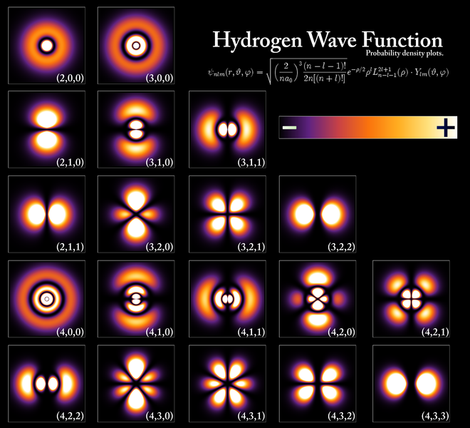
ψ(r, t) = e^{−i·(E/ħ)·t}·ψ(r)

We might say the ψ(r) function is sort of an envelope function for the whole wavefunction, but it’s not quite as straightforward as that. However, I am sure you’ll figure it out.

States with an angular dependence

So far, so good. But what if those partial derivatives are not zero? Now the calculations become really complicated. Among other things, we need these transformation matrices for rotations, which we introduced a very long time ago. As mentioned above, I don’t have the intention to copy Feynman here, who needs another two or three dense pages to work out the logic. Let me just state the grand result:

We’ve got a whole range of definite energy states, which correspond to orbitals that form an orthonormal basis for the actual wavefunction of the electron.
The orbitals are characterized by three quantum numbers, denoted as l, n and m respectively:
- The l is the quantum number of (total) angular momentum, and it’s equal to 0, 1, 2, 3, etcetera. [Of course, as usual, we’re measuring in units of ħ.] The l = 0 states are referred to as s-states, the l = 1 states are referred to as p-states, and the l = 2 states are d-states. They are followed by f, g, h, etcetera—for no particular good reason. [As Feynman notes: “The letters don’t mean anything now. They did once—they meant “sharp” lines, “principal” lines, “diffuse” lines and “fundamental” lines of the optical spectra of atoms. But those were in the days when people did not know where the lines came from. After f there were no special names, so we now just continue with g, h, and so on.]
- The m is referred to as the ‘magnetic’ quantum number, and it ranges from −l to +l.
- The n is the ‘principle’ quantum number, and it goes from l + 1 to infinity (∞).

How do these things actually look like? Let me insert two illustrations here: one from Feynman, and the other from Wikipedia.

shape

The number in front just tracks the number of s-, p-, d-, etc. orbital. The shaded region shows where the amplitudes are large, and the plus and minus signs show the relative sign of the amplitude. [See my remark above on the fact that the ψ factor is real-valued, even if the wavefunction as a whole is complex-valued.] The Wikipedia image shows the same density plots but, as it was made some 50 years later, with some more color. 🙂

660px-Hydrogen_Density_Plots

This is it, guys. Feynman takes it further by also developing the electron configurations for the next 35 elements in the periodic table but… Well… I am sure you’ll want to read the original here, rather than my summaries. 🙂

Congrats ! We now know all what we need to know. All that remains is lots of practical exercises, so you can be sure you master the material for your exam. 🙂

Some content on this page was disabled on June 16, 2020 as a result of a DMCA takedown notice from The California Institute of Technology. You can learn more about the DMCA here:

https://wordpress.com/support/copyright-and-the-dmca/
Some content on this page was disabled on June 16, 2020 as a result of a DMCA takedown notice from The California Institute of Technology. You can learn more about the DMCA here:

https://wordpress.com/support/copyright-and-the-dmca/
Some content on this page was disabled on June 16, 2020 as a result of a DMCA takedown notice from The California Institute of Technology. You can learn more about the DMCA here:

https://wordpress.com/support/copyright-and-the-dmca/
Some content on this page was disabled on June 16, 2020 as a result of a DMCA takedown notice from The California Institute of Technology. You can learn more about the DMCA here:

https://wordpress.com/support/copyright-and-the-dmca/
Some content on this page was disabled on June 16, 2020 as a result of a DMCA takedown notice from The California Institute of Technology. You can learn more about the DMCA here:

https://wordpress.com/support/copyright-and-the-dmca/
Some content on this page was disabled on June 16, 2020 as a result of a DMCA takedown notice from The California Institute of Technology. You can learn more about the DMCA here:

https://wordpress.com/support/copyright-and-the-dmca/