Pre-scriptum (dated 26 June 2020): This post – part of a series of rather simple posts on elementary math and physics – did not suffer much from the attack by the dark force—which is good because I still like it. Enjoy !
Original post:
This will surely be not my most readable post – if only because it’s soooooo long and – at times – quite ‘philosophical’. Indeed, it’s not very rigorous or formal, unlike those posts on complex analysis I wrote last year. At the same time, I think this post digs ‘deeper’, in a sense. Indeed, I really wanted to get to the heart of the ‘magic’ behind complex numbers. I’ll let you judge if I achieved that goal.
Complex numbers: why are they useful?
The previous post demonstrated the power of complex numbers (i.e. why they are used for), but it didn’t say much about what they are really. Indeed, we had a simple differential equation–an expression modeling an oscillator (read: a spring with a mass on it), with two terms only: d2x/dt2 = –ω2x–but so we could not solve it because of the minus sign in front of the term with the x.
Indeed, the so-called characteristic equation for this differential equation is r2 = –ω2 and so we’re in trouble here because there is no real-valued r that solves this. However, allowing complex-valued roots (r = ±iω) to solve the characteristic equation does the trick. Let’s analyze what we did (and don’t worry if you don’t ‘get’ this: it’s not essential to understand what follows):
- Using those complex roots, we wrote the general solution for the differential equation as Aeiωt+ Be–iωt. Now, note that everything is complex in this general solution, not only the eiωt and e–iωt ‘components’ but also the (random) coefficients A and B.
- However, because we wanted to find a real-valued function in the end (remember: x is a vertical displacement from an equilibrium position x = 0, so that’s ‘real’ indeed), we imposed the condition that Aeiωtand Be–iωt had to be each other’s complex conjugate. Hence, B must beequal to A* and our ‘general’ (real-valued) solution was Aeiωt+ A*e–iωt. So we only have one complex (but equally random) coefficient now – A – and we get the other one (A*) for free, so to say.
- Writing A in polar notation, i.e. substituting A for A = x0eiΔ, which implies that A* = x0e–iΔ, yields A0eiΔeiωt + A0e-iΔe–iω = A0[ei(ωt + Δ) + e–i(ωt + Δ)].
- Expanding this, using Euler’s formula (and the fact that cos(-α) = cosα but sin(-α) = –sinα) then gives us, finally, the following (real-valued) functional form for x:
A0[cos(ωt + Δ) + isin(ωt + Δ) + cos(ωt + Δ) – isin(ωt + Δ)]
= 2A0cos(ωt + Δ) = x0cos(ωt + Δ)
That’s easy enough to follow, I guess (everything is relative of course), but do we really understand what we’re doing here? Let me rephrase what’s going on here:
- In the initial problem, our dependent variable x(t) was the vertical displacement, so that was a real-valued function of a real-valued (independent) variable (time).
- Now, we kept the independent variable t real – time is always real, never imaginary 🙂 – but so we made x = x(t) a complex (dependent) variable by equating x(t) with the complex-valued exponential ert. So we’re doing a substitution here really.
- Now, if ert is complex-valued, it means, of course, that r is complex and so that allows us to equate r with the square root of a negative number (r = ±iω).
- We then plug these imaginary roots back in and get a general complex-valued solution (as expected).
- However, we then impose the condition that the imaginary part of our solution should be zero.
In other words, we had a family of complex-valued functions as a general solution for the differential equation, but we limited the solution set to a somewhat less general solution including real-valued functions only.
OK. We all get this. But it doesn’t mean we ‘understand’ complex numbers. Let’s try to take the magic out of those complex numbers.
Complex numbers: what are they?
I’ve devoted two or three posts to this already (October-November 2013) but let’s go back to basics. Let’s start with that imaginary unit i. The essence of i – and, yes, I am using the term ‘essence’ in a very ‘philosophical’ sense here I guess: i‘s intrinsic nature, so to speak – is that its square is equal to minus one: i2= –1.
That’s it really. We don’t need more. Of course, we can associate i with lots of other things if we would want to (and we will, of course!), such as Euler’s formula for example, but these associations are not essential – or not as essential as this definition I should say. Indeed, while that ‘rule’ or ‘definition’ is totally weird and – at first sight – totally random, it’s the only one we need: all other arithmetic rules do not change and, in fact, it’s just that one extra rule that allows us to deal with any algebraic equation – so that’s literally every equation involving addition, multiplication and exponentiation (so that’s every polynomial basically). However, stating that i2= –1 still doesn’t answer the question: what is a complex number really?
In order to not get too confused, I’ve started to think we should just take complex numbers at face value: it’s the sum of (i) some real number and (ii) a so-called imaginary part, which consists of another real number multiplied with i. [So the only ‘imaginary’ bit is, once again, i: all the rest is real! ] Now, when I say the ‘sum’, then that’s not some kind of ‘new’ sum. Well… Let me qualify that. It’s not some kind of ‘new’ sum because we’re just adding two things the way we’re used to: two and two apples are four apples, and one orange plus two more is three. However, it is true that we’re adding two separate beasts now, so to say, and so we do keep the things with an i in them separate from the real bits. In short, we do keep the apples and the oranges separate.
Now, I would like to be able to say that multiplication of complex numbers is just as straightforward as adding them, but that’s not true. When we multiply complex numbers, that i2= –1 rule kicks in and produces some ‘effects’ that are logical but not all that ‘straightforward’ I’d say.
Let’s take a simple example–but a significant one (if only because we’ll use the result later): let’s multiply a complex number with itself, i.e. let’s take the square of a complex number. We get (a + bi)2= (a + bi)(a + bi) = a·a + a·(bi) + (bi)·a + (bi)·(bi) = a2 + 2abi + b2i2 = a2 + 2abi – b2. That’s very different as compared to the square of a real sum a + b: (a + b)2 = a2 + 2ab + b2. How? Just look at it: we’ve got a real bit (a2 – b2) and then an imaginary bit (2abi). So what?
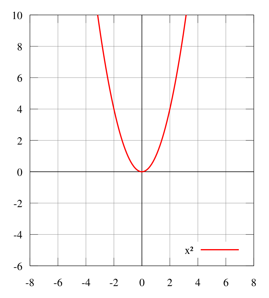
Well… The thumbnail graph below illustrates the difference for a = b: it maps x to (a) 4x2 [i.e. (x + x)2] and to (b) 2x2 [i.e. (x + ix)2] respectively. Indeed, when we’re squaring real numbers, we get (a + b)2 = 4a2–i.e. a ‘real bit’ only, of course!–but when we’re squaring complex numbers, we need to keep track of two components: the real part and the imaginary part. However, the real part (a2 – b2) is zero in this case (a = b), and so it’s only the imaginary part 2abi = 2a2i that counts!
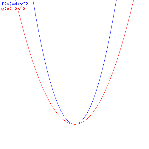
That’s kids stuff, you’ll say… In fact, when you’re a mathematician, you’ll say it’s a nonsensical graph. Why? Because it compares an apple and an orange really: we want to show 2ix2 really, not 2x2.
That’s true. However, that’s why the graph is actually useful. The red graph introduces a new idea, and with a ‘new’ idea I mean something that’s not inherent in the i2= –1 identity: it associates i with the vertical axis in the two-dimensional plane.
Hmm… This is an idea that is ‘nice’ – very nice actually – but, once again, I should note that it’s not part of i‘s essence. Indeed, the Italian mathematicians who first ‘invented’ complex numbers in the early 16th century (Tartaglia (‘the Stammerer’) and da Vinci’s friend Cardano) introduced roots of –1 because they needed them to solve algebraic equations. That’s it. Full stop. It was only much later (some hundred years later that is!) that Euler and Descartes associated imaginary numbers (like 2ix2) with the vertical coordinate axis. To my readers who have managed not to fall asleep while reading this: please continue till the end, and you will understand why I am saying the idea of a geometrical interpretation is ‘not essential’.
To the same readers, I’ll also say the following, however: if we do associate complex numbers with a second dimension, then we can associate the algebraic operations with things we can visualize in space. Most of you–all of you I should say–know that already, obviously, but let’s just have a look at that to make sure we’re on the same page.
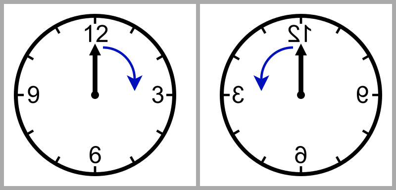
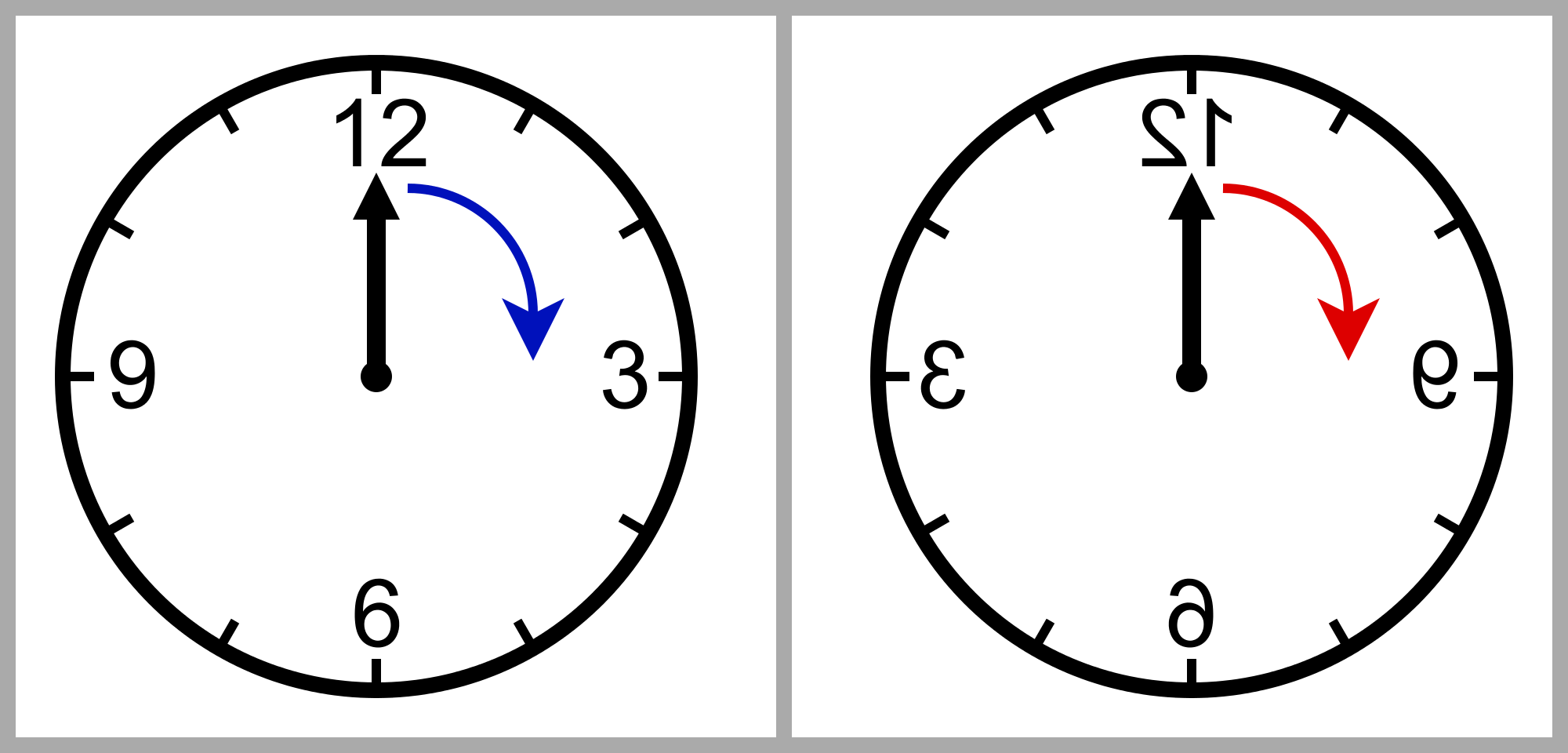
A very basic thing in physical mathematics is reversing the direction of something. Things go in one direction, but we should be able to visualize them going in the opposite direction. We may associate this with a variable going from 0 to infinity (+∞): it may be time (t), or a time-dependent variable x, y or z. Of course, we know what we have here: we think of the positive real axis. So, what we do when we multiply with –1 is reversing its direction, and so then we’re talking the negative real axis: a variable going from 0 to minus infinity (-∞). Therefore, we can associate multiplication by –1 with a full rotation around the center (i.e. around the zero point) by 180 degrees (i.e. by π, in radians).
You may think that’s a weird way of looking at multiplication by minus one. Well… Yes and no. But think of it: the concept of negative numbers is actually as ‘weird’ as the concept of the imaginary unit in a way. I mean… Think about it: we’re used to use negative numbers because we learned about them when we were very small kids but what are they really? What does it mean to have minus three apples? You know the answer of course: it probably means that you owe someone three apples but that you don’t have any right now. 🙂 […] But that’s not the point here. I hope you see what I mean: negative numbers are weird too, in a sense. Indeed, we should be aware of the fact that we often look at concepts as being ‘weird’ because we weren’t exposed to them early enough: the great mathematician Leonhard Euler thought complex numbers were so ‘essential’ to math and, hence, so ‘natural’ that he thought kids should learn complex numbers as soon as they started learning ‘real’ numbers. In fact, he probably thought we should only be using complex numbers because… Well… They make the arithmetic space complete, so to say. […] But then I guess that’s because Euler understood complex numbers in a way we don’t, which is why I am writing about them here. 🙂
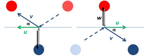
OK. Back to the main story line. In order to understand complex numbers somewhat better, it is actually useful – but, again, not necessarily essential – to think of i as a halfway rotation, i.e. a rotation by 90 degrees only, clockwise or counterclockwise, as illustrated above: multiplication with i means a counterclockwise rotation by 90 degrees (or π/2 radians) and multiplication with –i means a clockwise rotation by the same amount. Again, the minus sign gives the direction here: clockwise or counterclockwise. It works indeed: i·i =(-i)·(-i) = –1.
OK. Let’s wrap this up: we might say that
- a positive real number is associated with some (absolute) quantity (i.e. a magnitude);
- a minus sign says: “Go the opposite way! Go back! Subtract!”– so it’s associated with the opposite direction or the opposite of something in general; and, finally,
- the imaginary unit adds a second dimension: instead of moving on a line only, we can now walk around on a plane.
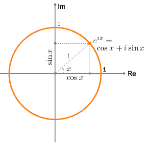
Once we understand that, it’s easy to understand why, in most applications of complex numbers, you’ll see the polar notation for complex numbers. Indeed, instead of writing a complex number z as z = a+ ib, we’ll usually see it written as:
z = reiθ with eiθ = cosθ + isinθ
Huh? Well… Yes. Let me throw it in here straight away. You know this formula: it’s Euler’s formula. The so-called ‘magical’ formula! Indeed, Feynman calls it ‘our jewel’: the ‘most remarkable formula in mathematics’ as he puts it. Waw ! If he says so, it must be right. 🙂 So let’s try to understand it.
Is it magical really? Well… I guess the answer is ‘Yes’ and ‘No’ at the same time:
- No. There is no ‘magic’ here. Associating the real part a and the imaginary part b with a magnitude r and an angle θ (a = rcosθ and b = rcosθ) is actually just an application of the Pythagorean theorem, so that’s ‘magic’ you learnt when you were very little and, hence, it does not look like magic anymore. [Although you should try to appreciate its ‘magic’ once again, I feel. Remember that you heard about the Pythagorean theorem because your teacher wanted to tell you what the square root of 2 actually is: a so-called irrational number that we get by taking the ‘one-half power’ of 2, i.e. 21/2 = 20.5, or, what amounts to the same, the square root of 2. Of course, you and I are both used to irrational numbers now, like 21/2, but they are also ‘weird’. As weird as i. In fact, it is said that the Greek mathematician who claimed their existence was exiled, because these irrational numbers did not fit into the (early) Pythagorean school of thought. Indeed, that school of thought wanted to reduce geometry to whole numbers and their ratios only. So there was no place for irrational numbers there!]
- Yes. It is ‘magical’. Associating eiθ – so that’s a complex exponential function really! – with the unit circle is something you learnt much later in life only, if ever. It’s a strange thing indeed: we have a real (but, I admit, irrational) number here – e is 2.718 followed by an infinite number of decimals as you know, just like π – and then we raise to the power iθ, so that’s i once again multiplied by a real number θ (i.e. the so-called phase or – to put it simply – the angle). By now, we know what it means to multiply something with i, and–of course–we also know what exponentiation is (it’s just a shorthand for repeated multiplication), but we haven’t defined complex exponentials yet.
In fact… That’s what we’re going to do here. But in a rather ‘weird’ way as you will see: we won’t define them really but we’ll calculate them. For the moment, however, we’ll leave it at this and just note that, through Euler’s relation, we can see how a fraction or a multiple of i, e.g. 0.1i or 2.3i, corresponds to a fraction or a multiple of the angle associated with i, i.e. 0.1 times π/2 or 2.3 times π/2. In other words, Euler’s formula shows how the second (spatial) dimension is associated with the concept of the angle.
[…] And then the third (spatial) dimension is, of course, easy to add: it’s just an angle in another direction. What direction? Well… An angle away from the plane that we just formed by introducing that first angle. 🙂 […] So, from our zero point (here and now), we use a ruler to draw lines, and then a compass to measure angles away from that line, and then we create a plane, and then we can just add dimensions as we please by adding more ‘angles’ away from what we already have (a line, or a plane, and any higher-dimensional thing really).
Dimensions
I feel I need to digress briefly here, just to make sure we’re on the same page. Dimensions. What is a dimension in physics or in math? What do we mean if we say that spacetime is a four-dimensional continuum? From what we wrote above, the concept of a spatial dimension should be obvious: we have three dimensions in space (the x, y and z direction), and so we need three numbers indeed to describe the position of an object, from our point of view that is (i.e. in our reference frame).
But so we also have a fourth number: time. By now, you also know that, just like position and/or motion in space, time is relative too: that is relative to some frame of reference indeed. So, yes, we need four numbers, i.e. four dimensions, to describe an event in spacetime. That being said, time is obviously still something different (I mean different than space), despite the fact that Einstein’s relativity theory relates it to space: indeed, we showed in our post on (special) relativity that there’s no such thing as absolute time. However, that actually reinforces the point: a point in time is something fundamentally different than a point in space. Despite the fact that
- Time is just like a space dimension in the physical-mathematical meaning of the term ‘dimension’ (a dimension of a space or an object is one of the coordinates that is needed to specify a point within that space, or to ‘locate’ the object – both in time and space that is); and that,
- We can express distance and time in the same units because the speed of light is absolute (so that allows us to express time in meter, despite the fact that time is relative or “local”, as Hendrik Lorentz called it); and that, finally,
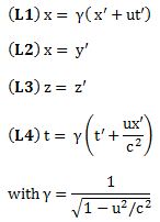
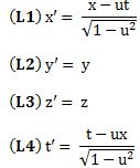
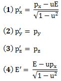
- If we do that (i.e. if we express time and distance in equivalent units), the equations for space and time in the Lorentz transformation equations mirror each other nicely – ‘mixing’ the space and time variables in the same way, so to say – and, therefore, space and time do form a ‘kind of union’, as Minkowski famously said;
Despite all that, time and space are fundamentally different things. Perhaps not for God – because He (or She, or It?) is said to be Everywhere Always – but surely for us, humans. For us, humans, always busy constructing that mental space with our ruler and our compass, time is and remains the one and only truly independent variable. Indeed, for us, mortal beings, the clocks just tick (locally indeed – that’s why I am using a plural: clocks – but that doesn’t change the fact they’re ticking, and in one direction only).
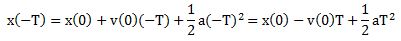
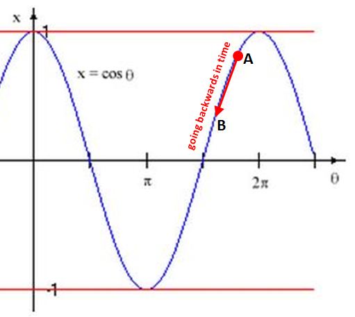
And so things happen and equations such as the one we started with – i.e. the differential equation modeling the behavior of an oscillator – show us how they happen. In one of my previous posts, I also showed why the laws of physics do not allow us to reverse time, but I won’t talk about that here. Let’s get back to complex numbers. Indeed, I am only talking about dimensions here because, despite all I wrote above about the imaginary axis in the complex plane, the thing to note here is that we did not use complex numbers in the physical-mathematical problem above to bring in an extra spatial dimension.
We just did it because we could not solve the equation with one-dimensional numbers only: we needed to take the square root of a negative number and we couldn’t. That was it basically. So there was no intention of bringing in a y- or z-dimension, and we didn’t. If we would have wanted to do that, we would have had to insert another dependent variable in the differential equation, and so it would have become a so-called partial differential equation in two or three dependent variables (x, y and z), with time – once again – as the independent variable (t). [A differential equation in one variable only (real- or complex-valued), like the ones we’re used to now, are referred to as ordinary differential equations, as opposed to… no, not extraordinary, but partial differential equations.]
In fact, if we would have generalized to two- or three-dimensional space, we would have run into the same type of problem (roots of negative numbers) when trying to solve the partial differential equation and so we would have needed complex-valued variables to solve it analytically in this case too. So we would have three ‘dimensions’ but each ‘dimension’ would be associated with complex (i.e. ‘two-dimensional) numbers. Is this getting complicated? I guess so.
The point is that, when studying physics or math, we will have to get used to the fact that these ‘two-dimensional numbers’ which we introduced, i.e. complex numbers, are actually more ‘natural’ ‘numbers’ to work with from a purely analytic point of view (as for the meaning of ‘analytic’, just read it as ‘logical problem-solving’), especially when we write them in their polar form, i.e. as complex exponentials. We can then take advantage of that wonderful property that they already are a functional form (z =reiθ), so to speak, and that their first, second etcetera derivative is easy to calculate because that ‘functional form’ is an exponential, and exponentials come back to themselves when taking the derivative (with the coefficient in the exponent in front). That makes the differential equation a simple algebraic equation (i.e. without derivatives involved), which is easy to solve.
In short, we should just look at complex numbers here (i.e. in the context of my three previous posts, or in the context of differential equations in general) as a computational device, not as an attempt to add an extra spatial dimension to the analysis.
Now, that’s probably the reason why Feynman inserts a chapter on ‘algebra’ that, at first, does not seem to make much sense. As usual, however, I worked through it and then found it to be both instructive as well as intriguing because it makes the point that complex exponentials are, first and foremost, an algebraic thing, not a geometrical thing.
I’ll try to present his argument here but don’t worry if you can’t or don’t want to follow it all the way through because… Well… It’s a bit ‘weird’ indeed, and I must admit I haven’t quite come to terms with it myself. On the other hand, if you’re ready for some thinking ‘outside of the box’, I assure you that I haven’t found anything like this in a math textbook or on the Web. This proves the fact that Feynman was a bit of a maverick… Well… In any case, I’ll let you judge. Now that you’re here, I would really encourage you to read the whole thing, as loooooooong as it is.
Complex exponentials from an algebraic point of view: introduction
Exponentiation is nothing but repeated multiplication. That’s easy to understand when the exponents are integers: a to the power n (an) is a×a×a×a×… etcetera – repeated n times, so we have n factors (all equal to a) in the product. That’s very straightforward.
Now, to understand rational exponents (so that’s an m/n exponent, with m and n integers), we just need to understand one thing more, and that is the inverse operation of exponentiation, i.e. the nth root. We then get am/n = (am)1/n. So, that’s easy too. […] Well… No. Not that easy. In fact, our problems starts right here:
- If n is even, and a is a positive real number, we have two (real) nth roots a1/n: ± a1/n.
- However, if a is negative (and n is still even obviously), then we have a problem. There’s no real nth root of a in that case. That’s why Cardano invented i: we’ll associate an even root of a negative real number with two complex-valued roots.
- What if n is uneven? Then we have only one real root: it’s positive when a is positive, and negative when a is negative. Done.
But let’s not complicate matters from the start. The point here is to do some algebra that should help us to understand complex exponentials. However, I will make one small digression, and that’s on logarithmic functions. It’s not essential but, again, useful. […] Well… Maybe. 🙂 I hope so. 🙂
We know that exponentials are actually associated with two inverse operations:
- Given some value y and some number n, we can take the nth root of y (y1/n) to find the original base x for which y = xn.
- Given some value y and some number a, we can take the logarithm (to base a) of y to find the original exponent x for which y = ax.
In the first case, the problem is: given n, find x for which y = xn. In the second case, the problem is: given a, find x for which y = ax. Is that complicated? Probably. In order to further confuse you, I’ve inserted a thumbnail graph with y = 2x (so that’s the exponential function with base 2) and y = log2x (so that’s the logarithmic function with base 2). You can see these two functions mirror each other, with the x = y line as the mirror axis.

We usually find logarithms more ‘difficult’ than roots (I do, for sure), but that’s just because we usually learn about them much later in life–like in a senior high school class, for example, as opposed to a junior high school class (I am just guessing, but you know what I mean).
In addition, we have these extra symbols ‘log‘–L-O-G :-)–to express the function. Indeed, we use just two symbols to write the y = 2x function: 2 and x – and then the meaning is clear from where we write these: we write 2 in normal script and x as a superscript and so we know that’s exponentiation. But so we’re not so economical for the logarithmic function. Not at all. In fact, we use three symbols for the logarithmic function: (1) ‘log’ (which is quite verbose as a symbol in itself, because it consists of three letters), (2) 2 and (3) x. That’s not economical at all! Indeed, why don’t we just write y = 2x or something? So that’s a subscript in front, instead of a superscript behind. It would work. It’s just a matter of getting used to it, i.e. it’s just a convention in other words.
Of course, I am joking a bit here but you get my point: in essence, the logarithmic function should not come across as being more ‘difficult’ or less ‘natural’ than the exponential function: exponentiation involves two numbers – a base and an exponent – and, hence, it’s logical that we have two inverse operations, rather than one. [You’ll say that a sum or a product involves (at least) two terms or two factors as well, so why don’t they have two inverse operations? Well… Addition and multiplication are commutative operations: a+b = b+a, and a·b = b·a. Exponentiation isn’t: an ≠ na. That’s why. Check it: 2×3 = 3×2, but 23 = 8 ≠ 32 = 9.]
Now, apart from us ‘liking’ exponential functions more than logarithmic functions because of the non-relevant fact that we learned about log functions only much later in our life, we will usually also have a strong preference for one or the other base for an exponential. The most preferred base is, obviously, ten (10). We use that base in so-called scientific notations for numbers. For example: the elementary charge (i.e. the charge of an electron) is approximately –1.6×10⁻¹⁹ coulombs. […] Oh… We have a minus sign in the exponent here (–19). So what’s that? Sorry. I forgot to mention that. But it’s easy: a–n = (an)–1 = 1/an.
Our most preferred base is 10 because we have a decimal system, and we have a decimal system because we have ten fingers. Indeed, the Maya used a base-20 system because they used their toes to count as well (so they counted in twenties instead of tens), and it also seems that some tribes had octal (base-8) systems because they used the spaces between their fingers, rather than the fingers themselves. And, of course, we all know that computers use a base-2 system because… Well… Because they’re computers. In any case, 10 is called the common base, because… Well… Because it’s common.
However, by now you know that, in physics and mathematics, we prefer that strange number e as a base. However, remember it’s not that strange: it’s just a number like π. Why do we call it ‘natural’? Because of that nice property: the derivative of the exponential function ex comes back to itself: d(ex)/dt = ex. That’s not the case for 10x. In fact, taking the derivative of 10x is pretty easy too: we just need to put a coefficient in front. To be specific, we need to put the logarithm (to base e) of the base of our exponential function (i.e. 10) in front: d(10x)/dt = 10xln(10). [Ln(10) is yet another notation that has been introduced, it seems, to confuse young kids and ensure they hate logarithms: ln(10) is just loge(10) or, if I would have had my way in terms of conventions (which would ensure an ‘economic’ use of symbols), we could also write ln(10) = e10. :-)]
Stop! I am going way too fast here. We first need to define what irrational powers are! Indeed, from all that I’ve written so far, you can imagine what am/n is (am/n = am)1/n, but what if m is not an integer? What if m equals the square root of 2, for example? In other words, what is 10x or ex or 2x or whatever for irrational exponents?
We all sort of ‘know’ what irrationals are: it involves limits, infinitesimals, fractions of fractions, Dedekind cuts. Whatever, even if you don’t understand a word of what I am writing here, you do – intuitively: irrationals can be approximated by fractions of fractions. The grand idea is that we divide some number by 2, and then we divide by 2 once again (so we divide by 4), and then once again (so we take 1/8), and again (1/16), and so on and so on. These are Dedekind cuts. Of course, dividing by two is a pretty random way of cutting things up. Why don’t we divide by three, or by four, for example? Well… It’s the same as with those other ‘natural’ numbers: we have to start somewhere and so this ‘binary’ way of cutting things up is probably the most ‘natural’. 🙂 [Have you noticed how many ‘natural’ numbers we’ve mentioned already: 10, e, π, 2… And one (1) itself of course. :-)]
So we’ll use something like Dedekind cuts for irrational powers as well. We’ll define them as a sort of limit (in fact, that’s exactly what they are) and so we have to find some approximation (or convergence) process that allows us to do so.
We’ll start with base 10 here because, as mentioned above, base 10 comes across as more ‘natural’ (or ‘common’) to us non-mathematicians than the so-called ‘natural’ base e. However, I should note that the base doesn’t matter much because it’s quite easy to switch from one base to another. Indeed, we can always write as = (bk)s = bks = bt with a = bk and t = k·s (as for k, k is obviously equal to logb(a). From this simple formula, you can see that changing base amounts to changing the horizontal scale: we replace s by t = k·s. That’s it. So don’t worry about our choice of base. 🙂
Complex exponentials from an algebraic point of view: well… Not the introduction 🙂
Ouf! So much stuff! But so here we go. We take base 10 and see how such an approximation of an irrational power of 10 (10x) looks like. Of course, we can write any irrational number x as some (positive or negative) integer plus an endless series of decimals after the zero (e.g. e = 2 + 0.7182818284590452… etc). So let’s just focus on numbers between 0 and 1 as for now (so we’ll take the integer out of the total, so to speak). In fact, before we start, I’ll cheat and show you the result, just to make sure you can follow the argument a bit.
 Yes. That’s how 10x looks like, but so we don’t know that yet because we don’t know what irrational powers are, and so we can’t make a graph like that–yet. We only know very general things right now, such as:
- 100 = 1 and 101 = 10 etcetera.
- Most importantly, we know that 10m/n = (10m)1/n = (101/n)m for integer m and n.
In fact, we’ll use the second fact to calculate 10x for x = 1/2, 1/4, 1/8, 1/16, and so on and so on. We’ll go all the way down to where x becomes a fraction very close to zero: that’s the table below. Note that the x values in the table are rational fractions 1/2, 1/4, 1/8 etcetera indeed, so x is not an irrational exponent: x is a real number but rational, so x can be expressed either as a fraction of two integers m and n (m = 1 and n = 1, 4, 8, 16, 32 and so on here), or as a decimal number with a finite number of decimals behind the decimal point (0.5, 0.25, 0.125, 0.0625 etcetera).

The third column gives the value 10x for these fractions x = 1/2, 1/4, 1/8 etcetera. How do we get these? Hmm… It’s true. I am jumping over another hurdle here. The key assumption behind the table is that we know how to take the square root of a number, so that we can calculate 101/2, to quite some precision indeed, as 101/2 = 3.162278 (and there’s more decimals but we’re not too interested in them right now), and then that we can take the square root of that value (3.162278). That’s quite an assumption indeed.
However, if we don’t want this post to become a book in itself, then I must assume we can do that. In fact, I’ve done it with a calculator here but, before there were calculators, this kind of calculations could and had to be done with a table of logarithms. That’s because of a very convenient property of logarithms: logc(ab) =logc(a) + logc(b). However, as said, I should be writing a post here only, not a book. [Already now, this post beats the record in terms of length and verbosity…] So I’ll just ask you to accept that – at this stage – we know how to calculate the square root of something and, therefore, to accept that we can take the square root not only of 10 but of any number really, including 3.162278, and then the root of that number, and then the root of that result, and so and so on. So that gives us the values in the third column of the table above: they’re successive square roots. [Please do double-check! It will help you to understand what I am writing about here.]
So… Back to the main story. What we are doing in the table above is to take the square root in succession, so that’s (101/2)1/2 = 101/4, and then again: (101/4)1/2 = 101/8 , and then again: (101/8)1/2 = 101/16 , so we get 101/2, 101/4, 101/8, 101/16, 101/32 and so on and so on. All the way down. Well… Not all the way down. In fact, in the table above, we stop after ten iterations already, so that’s when x = 1/1024. [Note that 1/1024 is 2 to the power minus 10: 2–10 = 1/210 = 1/1024. I am just throwing that in here because that little ‘fact’ will come in handy later.]
Why do we stop after ten iterations? Well… Actually, there’s no real good reason to stop at exactly ten iterations. We could have 15 iterations: then x would be 1/215 = 1/32768. Or 20 (x = 1/1048576). Or 39 (x = 1/too many digits to write down). Whatever. However, we start to notice something interesting that actually allows us to stop. We note that 10 to the power x (10x) tends to one as x becomes very small.
Now you’re laughing. Well… Surely ! That’s what we’d expect, isn’t it? 100 = 1. Is that the grand conclusion?
No.
The question is how small should x be? That’s where the fourth column of the table above comes in. We’re calculating a number there that converges to some value quite near to 2.3 as x goes to zero and – importantly – it converges rather quickly. In fact, if you’d do the calculations yourself, you’d see that it converges to 2.302585 after a while. [With Excel or some similar application, you can do 20 or more iterations in no time, and so that’s what you’ll find.]
Of course, we can keep going and continue adding zillions of decimals to this number but we don’t want to do that: 2.302585 is fine. We don’t need any more decimals. Why? Well… We’re going to use this number to approximate 10x near x = 0: it turns out that we can get a real good approximation of 10x near x = 0 using that 2.302585 factor, so we can write that
10x ≈ 1 + 2.302585x
That approximation is the last column in the table above. In order to show you how good it is as an ‘approximation’, I’ve plotted the actual values for 10x (blue markers) and the approximated values for 10x (black markers) using that 1 + 2.302585x formula. You can see it’s a pretty good match indeed if x is small. And ‘small’ here is not that small: a ratio like x = 1/8 (i.e. x = 0.125) is good enough already! In fact, the graph below shows that 1/16 = 0.0625 is almost perfect! So we don’t need to ‘go down’ too far: ten iterations is plenty!
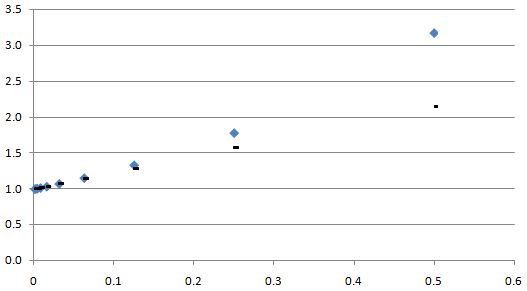
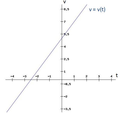
I’ve probably ‘lost’ you by now. What are we doing here really? How did we get that linear approximation formula, and why do we need it? Well… See the last column: we calculate (10x–1)/x, so that’s the difference between 10x and 1 divided by the (fractional) exponent x and we see, indeed, that that number converges to a value very near to 2.302585. Why? Well… What we are actually doing is calculating the gradient of 10x, i.e. the slope of the tangent line to the (non-linear) 10x curve. That’s what’s shown in the graph below.
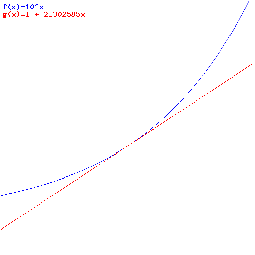
Working backwards, we can then re-write (10x–1)/x ≈ 2.302585 as 10x ≈ 1 + 2.302585x indeed.
So what we’ve got here is quite standard: we know we can approximate a non-linear curve with a linear curve, using the gradient near the point that we’re observing (and so that’s near the point x = 0 in this case) and so that‘s what we’re doing here.
Of course, you should remember that we cannot actually plot a smooth curve like that, for the moment that is, because we can only calculate 10x for rational real numbers. However, it’s easy to generalize and just ‘fill the gaps’ so to speak, and so that’s how irrational powers are defined really.
Hmm… So what’s the next step? Well… The next step is not to continue and continue and continue and continue etcetera to show that the smooth curve above is, indeed, the graph of 10x. No. The next step is to use that linear approximation to algebraically calculate the value of 10is, so that’s a power of 10 with a complex exponent.
HUH!?
Yes. That’s the gem I found in Feynman’s 1965 Lectures. [Well… One of the gems, I should say. There are many. :-)]
It’s quite interesting. In his little chapter on ‘algebra’ (Lectures, I-22), Feynman just assumes that this ‘law’ that 10x = 1 + 2.302585x is not only ‘correct’ for small real fractions x but also for very small complex fractions, and then he just reverses the procedure above to calculate 10ix for larger values of x. Let’s see how that goes.
However, let’s first switch the variable from x to s, because we’re talking complex numbers now. Indeed, I can’t use the symbol x as I used it above anymore because x is now the real part of some complex number 10is. In addition, I should note that Feynman introduces this delta (Δ). The idea behind is to make things somewhat easier to read by relating s to an integer: Δ = 1024s, so Δ = 1, 2, 4, 8,… 1024 for s = 1/1024, 1/512, 1/256 etcetera (see the second column in the table below). I am not entirely sure why he does that: Feynman must think fractions are harder to ‘read’. [Frankly, the introduction of this Δ makes Feynman’s exposé somewhat harder to ‘read’ IMHO – but that’s just a matter of taste, I guess.] Of course, the approximation then becomes
10x = 1 + 2.302585·Δ/1024 = 1 + 0.0022486Δ.
The table below is the one that Feynman uses. The important thing is that you understand the first line in this table: 10i/1024 = 1 + 0.00225i·Δ = 1 + 0.00225i·1 = 1 + 0.00225i. And then we go to the second line: 10i/512 = 10i/1024·10i/1024 = 102i/1024 = 10i/512, so we’re doing the reverse thing here: we don’t take square roots but we square what we’ve found already. So we multiply 1 + 0.00225i with itself and get (1+0.00225i)(1+0.00225i) = 1 + 2·0.00225i + 0.002252i2 = 1 – 0.000005 + 0.45i ≈ 0.999995 + 0.45i ≈ 1 + 0.0045i.

Let’s go to the third line now. In fact, what we’re doing here is working our way back up, i.e. all the way from s = 1/1024 to s = 1. And that’s where the ‘magic’ of i (i.e. the fact that i2 = –1) is starting to show: (0.999995+0.0045i)2 = 0.99999 + 2·0.999995·0.0045i + 0.00452i2 = 0.99997 + 0.009i. So the real part of 10is is changing as well – it is decreasing in fact! Why is that? Because of the term with the i2 factor! [I write 0.99997 instead of 0.99996 because I round up here, while Feynman consistently rounds down.]
So now the game is clear: we take larger and larger fractions s (i/512, i/256, i/128, etcetera), and calculate 10is by squaring the previous result. After ten iterations, we get the grand result for s = i/1 = i:
10is = –0.66928 + 0.74332i (more or less that is)
Note the minus sign in front of the real part, and look at the intermediate values for x and y too. Isn’t that remarkable?
OK. Waw ! But… So what? What’s next?
Well… To graph 10is, we should not just keep squaring things because that amounts to doubling the exponent again and again and so that means the argument is just making larger and larger jumps along the positive real axis really (see that graph that I made above: the distance between the successive values of x gets larger and larger, and so that’s a bad recipe for a smooth graph).
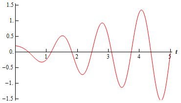
So what can we do? Well… We should just take a sufficiently small power, i/8 for example, and multiply that with 1, 2, 3 etcetera so we get something more ‘regular’. That’s what’s done in the table below and what’s represented in the graph underneath (to get the scale of the horizontal axis, note that s = p/8).

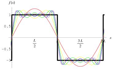
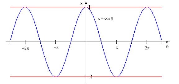
Hey! Look at that! There we are! That’s the graph we were looking for: it shows a (complex) exponential (10is) as a periodic (complex-valued) function with the real part behaving like a cosine function and the imaginary part behaving like as a sine function.
Note the upper and lower bounds: +1 and –1. Indeed, it doesn’t seem to matter whether we use 10 or e as a base: the x and y part oscillate between −1 and +1. So, whatever the base, we’ll see the same pattern: the base only changes the scale of the horizontal axis (i.e. s). However, that being said, because of this scale factor, I do need to say like a cosine/sine function when discussing that graph above. So I cannot say they are a cosine and a sine function. Feynman calls these functions algebraic sine and cosine functions.
But – remember! – we can always switch base through a clever substitution so 10is = eit and recalculate stuff to whatever number of decimals behind the decimal point we’d want. So let’s do that: let’s switch to base e. WOW! What happens?
We then [Finally! you’ll say!] get values that – Surprise ! Surprise ! – correspond to the real cosine and sine function. That then, in turn, allows us to just substitute the ‘algebraic’ cosine and sine function for the ‘real’ cosine in an equation that – Yes! – is Euler’s formula itself:
eit = cos(t) + isin(t)
So that’s it. End of story.
[…]
You’ll say: So what? Well… Not sure what to say. I think this is rather remarkable. This is not the formal mathematical proof of Euler’s formula (at least not of the kind that you’ll find in a textbook or on Wikipedia). No, we are just calculating the values x and y of eit = x + iy using an approximation process used to calculate real powers and then, well… Just some bold assumption involving infinitesimals really.
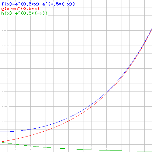
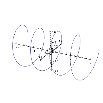
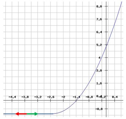
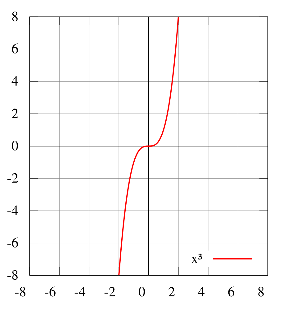
I think this is amazing stuff (even if I’ll downplay that statement a bit in my post scriptum). I really don’t understand these things the way I would like to understand them. I guess I just haven’t got the right kind of brain for these things. 😦 Indeed, just think about it: when we have the real exponential ex, then we’ve got that typical ‘rocket’ graph (i.e. the blue one in the graph below): just something blasting away indeed. But when we put i in the exponent (eix), then we get two components oscillating up and down like the cosine and sine function. Well… Not only like the cosine and sine function: the green and red line– i.e. the real and imaginary part of eix!– actually are the cosine and sine function!

Do you understand this in an intuitive way? Yes? You do? Waw ! Please write me and tell me how. I don’t. 😦
Oh well… The good thing about it is… Well… At least complex numbers will always stay ‘magical’ to me. 🙂
Post scriptum: When I write, above, that I don’t understand this in an intuitive way, I don’t mean to say it’s not logical. In fact, it is. It has to be, of course, because we’re talking math here! 🙂
The logic is pretty clear indeed. We have an exponential function here (y = 10x) and we’re evaluating that function in the neighborhood of x = 0 (we do it on the positive side only but we could, of course, do the same analysis on the other side as well). So then we use that very general mathematical procedure of calculating approximate values for the (non-linear) 10x curve using the gradient. So we plug in some differential value for x (in differential terms, we’d write Δx – but so the delta symbol here has nothing to do with Feynman’s Δ above) and, of course, we find Δy = 2.302585·Δx. So we add that to 1 (the value of 10x at point x = 0) and, then, we go through these iterations, not using that linear equation any more, but the very fundamental property of an exponential function that 102x = (10x)2. So we start with an approximate value, but then the value we plug into these iterative calculations is the square of the previous value. So, to calculate the next points, we do not use an approximation method any more, but we just square the first result, and then the second and so on and so on, and that’s just calculation, not approximation.
[In fact, you may still wonder and think that it’s quite remarkable that the points we calculate using this process are so accurate, but that’s due to the rapid convergence of that value we found for the gradient. Well… Yes and no. Here I must admit that Feynman (and I) cheated a bit because we used a rather precise value for the gradient: 2.302585, so that’s six significant digits after the decimal point. Now, that value is actually calculated based on twenty (rather than 10) iterations when ‘going down’. But that little factoid is not embarrassing because it doesn’t change much: the argument itself is sound. Very sound.]
OK… That’s easy enough to understand. The thing that is not easy to understand – intuitively that is – is that we can just insert some complex differential Δs into that Δy = 2.302585·Δx equation. Isn’t it ‘weird’, indeed, that we can just use a complex fraction i·s = i/1024 to calculate our first point, instead of a real fraction x = 1/1024? It is. That’s the only thing really. Indeed, once we’ve done that, it’s plain sailing again: we just square the result to get the next result, and then we square that again, and so on and so on. However, that being said, the difference is that the ‘magic’ of i comes into play indeed. When squaring, we do not get a 4a2 result but an (a+bi)2 = a2 – b2 + 2abi. So it’s that minus sign and the i that give an entirely different ‘dynamic’ to how the function evolves from there (i.e. different as compared to working with a real base only). It’s all quite remarkable really because we start off with a really tiny value b here: 0.00225 to be precise, so that’s (less than) 1/445 ! [Of course, the real part a, at the point from where we start doing these iterations, is one.]
But so that first step is ‘weird’ indeed. Why is it no problem whatsoever to insert the complex fraction s = i/1024 into 1 + 2.302585o·s, instead of the real fraction 1/1024, and then afterwards, to square these complex numbers that we’re getting, instead of real numbers?
It just doesn’t feel right, does it? I must admit that, at first, I felt that Feynman was doing something ‘illegal’ too. But, obviously, he’s not. It’s plain mathematical logic. We have two functions here: one is linear (y = 1 + 2.302585·x), and the other is quadratic (y = x2) and so what’s happening really is that, at the point x = 0, we change the function. We substitute not x for ix really but y = 10x for y = 10ix. So we still have an independent real variable x but, instead of a real-valued y = 10x function, we now have a complex-valued y = 10ix function.
However, the ‘output’ of that function, of course, is a complex y, not a real y. In our case, because we’re plotting a function really–to be precise, we’re calculating the exponential function y = 10x through all these iterations–we get a complex-valued function of the shape that, by now, we know so well.
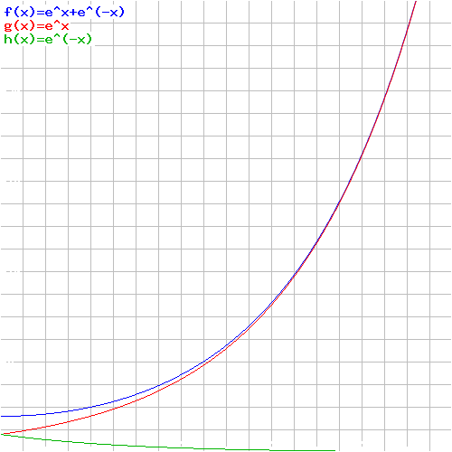
So it is ‘discontinuous’ in a way, and so I can’t say all that much about it. Look at the graph below where, once again, we have the real exponential function ex and then the two components of the complex exponential eix. This time, I’ve plotted them on both sides of the zero point because they’re continuous on both sides indeed. Imagine we’re walking along this blue ex curve from some negative x to zero. We’re familiar with the path. It has, for instance, that property we exploited above: as we doubled the ‘input’ (so from x we went to 2x), the ‘output’ went up not as the double but as the square of the original value: e2x = (ex)2. And then we also know that, around the point x = o, we can approximate it with a linear function. In fact, in this case, the linear approximation is super-simple: y = 1 + x. Indeed, the gradient for ex at point x = 0 is equal to 1! So, yes, we know and understand that blue curve. But then we arrive at point x = 0 and we decide something radical: we change the function!

Yes. That’s what we’re really doing in that very lengthy story above: eix is a complex-valued function of the real variable x. That’s something different. However, we continue to say that the approximation y = 1 + x must also be valid for complex x and y. So we say that eix = 1 + ix. Is that wrong? No. Not at all. Functional forms are functional forms and gradients are gradients: d(eix)/dx = ieix, and ieix at x = 0 is equal to ie0 = i! Hence, eix = 1 + ix is a perfectly legitimate linear approximation. And then it’s just the same thing again: we use that iteration mechanism to calculate successive squares of complex numbers because, for complex exponentials as well, we have e2(ix) = (eix)2.
So. The ‘magic’ is a lot of ‘confusion’ really. The point to note is that we do have a different function here: eix and ex ‘look’ similar–it’s just that i, right?– but, in fact, when we replace x by ix in the exponent of e, that’s quite a radical change. We can use the same linear approximation at x = ix = 0 but then it’s over. Our blue graph stops: we’re no longer walking along it. I can’t even say it bifurcates, so to say, into the red and the green one, because it doesn’t. We’re talking apples and oranges indeed, and so the comparison is quickly done: they’re different. Full stop.
Is there any geometrical relationship between all these curves? Well… Yes and no. I can see one, at the very start: the gradient of our ex function at x = 0 is equal to unity (i.e. 1), and so that’s the same gradient as the gradient of the imaginary part of our new eix function (the gradient of the real part is zero, before it becomes negative). But that’s just… I mean… That just comes out of Euler’s formula: e0 = cos(0) + isin(0). Honestly, it’s no use to try to be smart here and think about stuff like that. We’re no longer walking on the blue curve. We’re looking at a new function: a complex-valued function eix (instead of a real-valued function ex) of a real variable (x). That’s it. Just don’t try to relate the two too much: you switched functions. Full stop. It’s like changing trains! 🙂
So… What’s the conclusion? Well… I’d say: “Complex numbers can be analyzed as extensions of real numbers, so to say, but – frankly – they are different.”
[…]
I’ll probably never understand complex numbers in the way I would like to understand them–that is like I understand that one plus one is two. However, this rather lengthy forage in the complex forest has helped me somewhat. I hope it helped you too.
Some content on this page was disabled on June 16, 2020 as a result of a DMCA takedown notice from The California Institute of Technology. You can learn more about the DMCA here:
https://wordpress.com/support/copyright-and-the-dmca/
Some content on this page was disabled on June 16, 2020 as a result of a DMCA takedown notice from The California Institute of Technology. You can learn more about the DMCA here:https://wordpress.com/support/copyright-and-the-dmca/
Some content on this page was disabled on June 16, 2020 as a result of a DMCA takedown notice from The California Institute of Technology. You can learn more about the DMCA here:


 As for the constants in this formula, you know these by now: the speed of light c, the electron charge e, its mass me, and the permittivity of free space εe. For whatever it’s worth (because you should note that, in quantum mechanics, electrons do not have a size: they are treated as point-like particles, so they have a point charge and zero dimension), that’s small. It’s in the femtometer range (1 fm = 1