Re-visiting electron orbitals (III)

Pre-script (dated 26 June 2020): Our ideas have evolved into a full-blown realistic (or classical) interpretation of all things quantum-mechanical. In addition, I note the dark force has amused himself by removing some material. So no use to read this. Read my recent papers instead. 🙂

Original post:

In my previous post, I mentioned that it was not so obvious (both from a physical as well as from a mathematical point of view) to write the wavefunction for electron orbitals – which we denoted as ψ(x, t), i.e. a function of two variables (or four: one time coordinate and three space coordinates) – as the product of two other functions in one variable only.

[…] OK. The above sentence is difficult to read. Let me write in math. 🙂 It is not so obvious to write ψ(x, t) as:

ψ(x, t) = e^{−i·(E/ħ)·t}·ψ(x)

As I mentioned before, the physicists’ use of the same symbol (ψ, psi) for both the ψ(x, t) and ψ(x) function is quite confusing – because the two functions are very different:

ψ(x, t) is a complex-valued function of two (real) variables: x and t. Or four, I should say, because x = (x, y, z) – but it’s probably easier to think of x as one vector variable – a vector-valued argument, so to speak. And then t is, of course, just a scalar variable. So… Well… A function of two variables: the position in space (x), and time (t).
In contrast, ψ(x) is a real-valued function of one (vector) variable only: x, so that’s the position in space only.

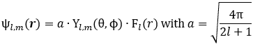
Now you should cry foul, of course: ψ(x) is not necessarily real-valued. It may be complex-valued. You’re right. You know the formula: wavefunction Note the derivation of this formula involved a switch from Cartesian to polar coordinates here, so from x = (x, y, z) to r = (r, θ, φ), and that the function is also a function of the two quantum numbers l and m now, i.e. the orbital angular momentum (l) and its z-component (m) respectively. In my previous post(s), I gave you the formulas for Y_l,m(θ, φ) and F_l,m(r) respectively. F_l,m(r) was a real-valued function alright, but the Y_l,m(θ, φ) had that e^i·m·φ factor in it. So… Yes. You’re right: the Y_l,m(θ, φ) function is real-valued if – and only if – m = 0, in which case e^i·m·φ = 1. 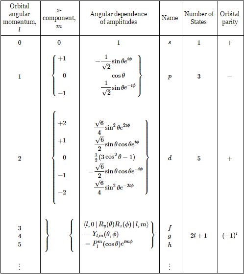Let me copy the table from Feynman’s treatment of the topic once again: spherical harmonics 2 The P_l^m(cosθ) functions are the so-called (associated) Legendre polynomials, and the formula for these functions is rather horrible:Don’t worry about it too much: just note the P_l^m(cosθ) is a real-valued function. The point is the following:the ψ(x, t) is a complex-valued function because – and only because – we multiply a real-valued envelope function – which depends on position only – with e^{−i·(E/ħ)·t}·e^i·m·φ = e^{−i·[(E/ħ)·t −}^m·φ].

[…]

Please read the above once again and – more importantly – think about it for a while. 🙂 You’ll have to agree with the following:

As mentioned in my previous post, the e^i·m·φ factor just gives us phase shift: just a re-set of our zero point for measuring time, so to speak, and the whole e^{−i·[(E/ħ)·t −}^m·φ] factor just disappears when we’re calculating probabilities.
The envelope function gives us the basic amplitude – in the classical sense of the word: the maximum displacement from the zero value. And so it’s that e^{−i·[(E/ħ)·t −}^m·φ] that ensures the whole expression somehow captures the energy of the oscillation.

Let’s first look at the envelope function again. Let me copy the illustration for n = 5 and l = 2 from a Wikimedia Commons article. Note the symmetry planes:

Any plane containing the z-axis is a symmetry plane – like a mirror in which we can reflect one half of the shape to get the other half. [Note that I am talking the shape only here. Forget about the colors for a while – as these reflect the complex phase of the wavefunction.]
Likewise, the plane containing both the x– and the y-axis is a symmetry plane as well.

n = 5

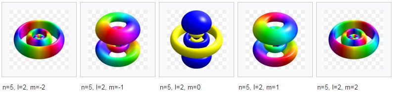
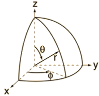
The first symmetry plane – or symmetry line, really (i.e. the z-axis) – should not surprise us, because the azimuthal angle φ is conspicuously absent in the formula for our envelope function if, as we are doing in this article here, we merge the e^i·m·φ factor with the e^{−i·(E/ħ)·t}, so it’s just part and parcel of what the author of the illustrations above refers to as the ‘complex phase’ of our wavefunction. OK. Clear enough – I hope. 🙂 But why is the the xy-plane a symmetry plane too? We need to look at that monstrous formula for the P_l^m(cosθ) function here: just note the cosθ argument in it is being squared before it’s used in all of the other manipulation. Now, we know that cosθ = sin(π/2 − θ). So we can define some new angle – let’s just call it α – which is measured in the way we’re used to measuring angle, which is not from the z-axis but from the xy-plane. So we write: cosθ = sin(π/2 − θ) = sinα. The illustration below may or may not help you to see what we’re doing here. angle 2 So… To make a long story short, we can substitute the cosθ argument in the P_l^m(cosθ) function for sinα = sin(π/2 − θ). Now, if the xy-plane is a symmetry plane, then we must find the same value for P_l^m(sinα) and P_l^m[sin(−α)]. Now, that’s not obvious, because sin(−α) = −sinα ≠ sinα. However, because the argument in that P_l^m(x) function is being squared before any other operation (like subtracting 1 and exponentiating the result), it is OK: [−sinα]² = [sinα]²= sin²α. […] OK, I am sure the geeks amongst my readers will be able to explain this more rigorously. In fact, I hope they’ll have a look at it, because there’s also that d^l+m/dx^l+m operator, and so you should check what happens with the minus sign there. 🙂

[…] Well… By now, you’re probably totally lost, but the fact of the matter is that we’ve got a beautiful result here. Let me highlight the most significant results:

A definite energy state of a hydrogen atom (or of an electron orbiting around some nucleus, I should say) appears to us as some beautifully shaped orbital – an envelope function in three dimensions, really – which has the z-axis – i.e. the vertical axis – as a symmetry line and the xy-plane as a symmetry plane.
The e^{−i·[(E/ħ)·t −}^m·φ] factor gives us the oscillation within the envelope function. As such, it’s this factor that, somehow, captures the energy of the oscillation.

It’s worth thinking about this. Look at the geometry of the situation again – as depicted below. We’re looking at the situation along the x-axis, in the direction of the origin, which is the nucleus of our atom.

spherical

The e^i·m·φ factor just gives us phase shift: just a re-set of our zero point for measuring time, so to speak. Interesting, weird – but probably less relevant than the e^{−i·[(E/ħ)·t} factor, which gives us the two-dimensional oscillation that captures the energy of the state.

Circle_cos_sin

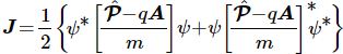
Now, the obvious question is: the oscillation of what, exactly? I am not quite sure but – as I explained in my Deep Blue page – the real and imaginary part of our wavefunction are really like the electric and magnetic field vector of an oscillating electromagnetic field (think of electromagnetic radiation – if that makes it easier). Hence, just like the electric and magnetic field vector represent some rapidly changing force on a unit charge, the real and imaginary part of our wavefunction must also represent some rapidly changing force on… Well… I am not quite sure on what though. The unit charge is usually defined as the charge of a proton – rather than an electron – but then forces act on some mass, right? And the mass of a proton is hugely different from the mass of an electron. The same electric (or magnetic) force will, therefore, give a hugely different acceleration to both.

So… Well… My guts instinct tells me the real and imaginary part of our wavefunction just represent, somehow, a rapidly changing force on some unit of mass, but then I am not sure how to define that unit right now (it’s probably not the kilogram!).

Now, there is another thing we should note here: we’re actually sort of de-constructing a rotation (look at the illustration above once again) in two linearly oscillating vectors – one along the z-axis and the other along the y-axis. Hence, in essence, we’re actually talking about something that’s spinning. In other words, we’re actually talking some torque around the x-axis. In what direction? I think that shouldn’t matter – that we can write E or −E, in other words, but… Well… I need to explore this further – as should you! 🙂

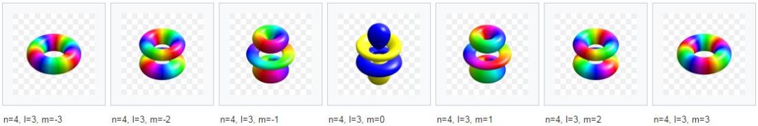
Let me just add one more note on the e^i·m·φ factor. It sort of defines the geometry of the complex phase itself. Look at the illustration below. Click on it to enlarge it if necessary – or, better still, visit the magnificent Wikimedia Commons article from which I get these illustrations. These are the orbitals n = 4 and l = 3. Look at the red hues in particular – or the blue – whatever: focus on one color only, and see how how – for m = ±1, we’ve got one appearance of that color only. For m = ±1, the same color appears at two ends of the ‘tubes’ – or tori (plural of torus), I should say – just to sound more professional. 🙂 For m = ±2, the torus consists of three parts – or, in mathematical terms, we’d say the order of its rotational symmetry is equal to 3. Check that Wikimedia Commons article for higher values of n and l: the shapes become very convoluted, but the observation holds. 🙂

l = 3

Have fun thinking all of this through for yourself – and please do look at those symmetries in particular. 🙂

Post scriptum: You should do some thinking on whether or not these m = ±1, ±2,…, ±l orbitals are really different. As I mentioned above, a phase difference is just what it is: a re-set of the t = 0 point. Nothing more, nothing less. So… Well… As far as I am concerned, that’s not a real difference, is it? 🙂 As with other stuff, I’ll let you think about this for yourself.

Some content on this page was disabled on June 17, 2020 as a result of a DMCA takedown notice from Michael A. Gottlieb, Rudolf Pfeiffer, and The California Institute of Technology. You can learn more about the DMCA here:

https://wordpress.com/support/copyright-and-the-dmca/

Feynman’s Seminar on Superconductivity (1)

Pre-script (dated 26 June 2020): This post got mutilated by the removal of some material by the dark force. You should be able to follow the main story line, however. If anything, the lack of illustrations might actually help you to think things through for yourself. In any case, we now have different views on these concepts as part of our realist interpretation of quantum mechanics, so we recommend you read our recent papers instead of these old blog posts.

Original post:

The ultimate challenge for students of Feynman’s iconic Lectures series is, of course, to understand his final one: A Seminar on Superconductivity. As he notes in his introduction to this formidably dense piece, the text does not present the detail of each and every step in the development and, therefore, we’re not supposed to immediately understand everything. As Feynman puts it: we should just believe (more or less) that things would come out if we would be able to go through each and every step. Well… Let’s see. Feynman throws a lot of stuff in here—including, I suspect, some stuff that may not be directly relevant, but that he sort of couldn’t insert into all of his other Lectures. So where do we start?

It took me one long maddening day to figure out the first formula:It says that the amplitude for a particle to go from a to b in a vector potential (think of a classical magnetic field) is the amplitude for the same particle to go from a to b when there is no field (A = 0) multiplied by the exponential of the line integral of the vector potential times the electric charge divided by Planck’s constant. I stared at this for quite a while, but then I recognized the formula for the magnetic effect on an amplitude, which I described in my previous post, which tells us that a magnetic field will shift the phase of the amplitude of a particle with an amount equal to:

Hence, if we write 〈b|a〉 for A = 0 as 〈b|a〉_{A = 0} = C·eⁱ^θ, then 〈b|a〉 in A will, naturally, be equal to 〈b|a〉 _{in A}= C·eⁱ⁽^θ+φ) = C·eⁱ^θ·eⁱ^φ = 〈b|a〉_{A = 0}·eⁱ^φ, and so that explains it. 🙂 Alright… Next. Or… Well… Let us briefly re-examine the concept of the vector potential, because we’ll need it a lot. We introduced it in our post on magnetostatics. Let’s briefly re-cap the development there. In Maxwell’s set of equations, two out of the four equations give us the magnetic field: ∇•B = 0 and c²∇×B = j/ε₀. We noted the following in this regard:

The ∇•B = 0 equation is true, always, unlike the ∇×E = 0 expression, which is true for electrostatics only (no moving charges). So the ∇•B = 0 equation says the divergence of B is zero, always.
The divergence of the curl of a vector field is always zero. Hence, if A is some vector field, then div(curl A) = ∇•(∇×A) = 0, always.
We can now apply another theorem: if the divergence of a vector field, say D, is zero—so if ∇•D = 0—then $D will be the$ the curl of some other vector field $C, so we can write: D = \nabla \times C . Applying this to \nabla • B = 0, we can write:$

If ∇•B = 0, then there is an A such that B = ∇×A

So, in essence, we’re just re-defining the magnetic field (B) in terms of some other vector field. To be precise, we write it as the curl of some other vector field, which we refer to as the (magnetic) vector potential. The components of the magnetic field vector can then be re-written as:

We need to note an important point here: the equations above suggest that the components of B depend on position only. In other words, we assume static magnetic fields, so they do not change with time. That, in turn, assumes steady currents. We will want to extend the analysis to also include magnetodynamics. It complicates the analysis but… Well… Quantum mechanics is complicated. Let us remind ourselves here of Feynman’s re-formulation of Maxwell’s equations as a set of two equations (expressed in terms of the magnetic (vector) and the electric potential) only:

Wave equation for A

Wave equation for potential

These equations are wave equations, as you can see by writing out the second equation:

It is a wave equation in three dimensions. Note that, even in regions where we do no have any charges or currents, we have non-zero solutions for φ and A. These non-zero solutions are, effectively, representing the electric and magnetic fields as they travel through free space. As Feynman notes, the advantage of re-writing Maxwell’s equations as we do above, is that the two new equations make it immediately apparent that we’re talking electromagnetic waves, really. As he notes, for many practical purposes, it will still be convenient to use the original equations in terms of E and B, but… Well… Not in quantum mechanics, it turns out. As Feynman puts it: “E and B are on the other side of the mountain we have climbed. Now we are ready to cross over to the other side of the peak. Things will look different—we are ready for some new and beautiful views.”

Well… Maybe. Appreciating those views, as part of our study of quantum mechanics, does take time and effort, unfortunately. 😦

The Schrödinger equation in an electromagnetic field

Feynman then jots down Schrödinger’s equation for the same particle (with charge q) moving in an electromagnetic field that is characterized not only by the (scalar) potential Φ but also by a vector potential A:

schrodinger

Now where does that come from? We know the standard formula in an electric field, right? It’s the formula we used to find the energy states of electrons in a hydrogen atom:

i·ħ·∂ψ/∂t = −(1/2)·(ħ²/m)∇²ψ + V·ψ

Of course, it is easy to see that we replaced V by q·Φ, which makes sense: the potential of a charge in an electric field is the product of the charge (q) and the (electric) potential (Φ), because Φ is, obviously, the potential energy of the unit charge. It’s also easy to see we can re-write −ħ²·∇²ψ as [(ħ/i)·∇]·[(ħ/i)·∇]ψ because (1/i)·(1/i) = 1/i² = 1/(−1) = −1. 🙂 Alright. So it’s just that −q·A term in the (ħ/i)∇ − q·A expression that we need to explain now.

Unfortunately, that explanation is not so easy. Feynman basically re-derives Schrödinger’s equation using his trade-mark historical argument – which did not include any magnetic field – with a vector potential. The re-derivation is rather annoying, and I didn’t have the courage to go through it myself, so you should – just like me – just believe Feynman when he says that, when there’s a vector potential – i.e. when there’s a magnetic field – then that (ħ/i)·∇ operator – which is the momentum operator– ought to be replaced by a new momentum operator:

new-momentum-operator

So… Well… There we are… 🙂 So far, so good? Well… Maybe.

While, as mentioned, you won’t be interested in the mathematical argument, it is probably worthwhile to reproduce Feynman’s more intuitive explanation of why the operator above is what it is. In other words, let us try to understand that −qA term. Look at the following situation: we’ve got a solenoid here, and some current I is going through it so there’s a magnetic field B. Think of the dynamics while we turn on this flux. Maxwell’s second equation (∇×E = −∂B/∂t) tells us the line integral of E around a loop will be equal to the time rate of change of the magnetic flux through that loop. The ∇×E = −∂B/∂t equation is a differential equation, of course, so it doesn’t have the integral, but you get the idea—I hope. solenoid

Now, using the B = ∇×A equation we can re-write the ∇×E = −∂B/∂t as ∇×E = −∂(∇×A)/∂t. This allows us to write the following:

∇×E = −∂(∇×A)/∂t = −∇×(∂A/∂t) ⇔ E = −∂A/∂t

This is a remarkable expression. Note its derivation is based on the commutativity of the curl and time derivative operators, which is a property that can easily be explained: if we have a function in two variables—say x and t—then the order of the derivation doesn’t matter: we can first take the derivative with respect to x and then to t or, alternatively, we can first take the time derivative and then do the ∂/∂x operation. So… Well… The curl is, effectively, a derivative with regard to the spatial variables. OK. So what? What’s the point?

Well… If we’d have some charge q, as shown in the illustration above, that would happen to be there as the flux is being switched on, it will experience a force which is equal to F = qE. We can now integrate this over the time interval (t) during which the flux is being built up to get the following:

∫₀^t F = ∫₀^t m·a = ∫₀^t m·dv/dt = m·v_t= ∫₀^t q·E = −∫₀^t q·∂A/∂t = −q·A_t

Assuming v₀ and A₀are zero, we may drop the time subscript and simply write:

m·v = −q·A

The point is: during the build-up of the magnetic flux, our charge will pick up some (classical) momentum that is equal to p = m·v = −q·A. So… Well… That sort of explains the additional term in our new momentum operator.

Note: For some reason I don’t quite understand, Feynman introduces the weird concept of ‘dynamical momentum’, which he defines as the quantity m·v + q·A, so that quantity must be zero in the analysis above. I quickly googled to see why but didn’t invest too much time in the research here. It’s just… Well… A bit puzzling. I don’t really see the relevance of his point here: I am quite happy to go along with the new operator, as it’s rather obvious that introducing changing magnetic fields must, obviously, also have some impact on our wave equations—in classical as well as in quantum mechanics.

Local conservation of probability

The title of this section in Feynman’s Lecture (yes, still the same Lecture – we’re not switching topics here) is the equation of continuity for probabilities. I find it brilliant, because it confirms my interpretation of the wave function as describing some kind of energy flow. Let me quote Feynman on his endeavor here:

“An important part of the Schrödinger equation for a single particle is the idea that the probability to find the particle at a position is given by the absolute square of the wave function. It is also characteristic of the quantum mechanics that probability is conserved in a local sense. When the probability of finding the electron somewhere decreases, while the probability of the electron being elsewhere increases (keeping the total probability unchanged), something must be going on in between. In other words, the electron has a continuity in the sense that if the probability decreases at one place and builds up at another place, there must be some kind of flow between. If you put a wall, for example, in the way, it will have an influence and the probabilities will not be the same. So the conservation of probability alone is not the complete statement of the conservation law, just as the conservation of energy alone is not as deep and important as the local conservation of energy. If energy is disappearing, there must be a flow of energy to correspond. In the same way, we would like to find a “current” of probability such that if there is any change in the probability density (the probability of being found in a unit volume), it can be considered as coming from an inflow or an outflow due to some current.”

This is it, really ! The wave function does represent some kind of energy flow – between a so-called ‘real’ and a so-called ‘imaginary’ space, which are to be defined in terms of directional versus rotational energy, as I try to point out – admittedly: more by appealing to intuition than to mathematical rigor – in that post of mine on the meaning of the wavefunction.

So what is the flow – or probability current as Feynman refers to it? Well… Here’s the formula:

probability-current-2

Huh? Yes. Don’t worry too much about it right now. The essential point is to understand what this current – denoted by J – actually stands for:

probability-current-1

So what’s next? Well… Nothing. I’ll actually refer you to Feynman now, because I can’t improve on how he explains how pairs of electrons start behaving when temperatures are low enough to render Boltzmann’s Law irrelevant: the kinetic energy that’s associated with temperature can no longer break up electron pairs if temperature comes close to the zero point.

Huh? What? Electron pairs? Electrons are not supposed to form pairs, are they? They carry the same charge and are, therefore, supposed to repel each other. Well… Yes and no. In my post on the electron orbitals in a hydrogen atom – which just presented Feynman’s presentation on the subject-matter in a, hopefully, somewhat more readable format – we calculated electron orbitals neglecting spin. In Feynman’s words:

“We make another approximation by forgetting that the electron has spin. […] The non-relativistic Schrödinger equation disregards magnetic effects. [However] Small magnetic effects [do] occur because, from the electron’s point-of-view, the proton is a circulating charge which produces a magnetic field. In this field the electron will have a different energy with its spin up than with it down. [Hence] The energy of the atom will be shifted a little bit from what we will calculate. We will ignore this small energy shift. Also we will imagine that the electron is just like a gyroscope moving around in space always keeping the same direction of spin. Since we will be considering a free atom in space the total angular momentum will be conserved. In our approximation we will assume that the angular momentum of the electron spin stays constant, so all the rest of the angular momentum of the atom—what is usually called “orbital” angular momentum—will also be conserved. To an excellent approximation the electron moves in the hydrogen atom like a particle without spin—the angular momentum of the motion is a constant.”

To an excellent approximation… But… Well… Electrons in a metal do form pairs, because they can give up energy in that way and, hence, they are more stable that way. Feynman does not go into the details here – I guess because that’s way beyond the undergrad level – but refers to the Bardeen-Coopers-Schrieffer (BCS) theory instead – the authors of which got a Nobel Prize in Physics in 1972 (that’s a decade or so after Feynman wrote this particular Lecture), so I must assume the theory is well accepted now. 🙂

Of course, you’ll shout now: Hey! Hydrogen is not a metal! Well… Think again: the latest breakthrough in physics is making hydrogen behave like a metal. 🙂 And I am really talking the latest breakthrough: Science just published the findings of this experiment last month! 🙂 🙂 In any case, we’re not talking hydrogen here but superconducting materials, to which – as far as we know – the BCS theory does apply.

So… Well… I am done. I just wanted to show you why it’s important to work your way through Feynman’s last Lecture because… Well… Quantum mechanics does explain everything – although the nitty-gritty of it (the Meissner effect, the London equation, flux quantization, etc.) are rather hard bullets to bite. 😦

Don’t give up ! I am struggling with the nitty-gritty too ! 🙂

Some content on this page was disabled on June 16, 2020 as a result of a DMCA takedown notice from The California Institute of Technology. You can learn more about the DMCA here:

https://wordpress.com/support/copyright-and-the-dmca/
Some content on this page was disabled on June 16, 2020 as a result of a DMCA takedown notice from The California Institute of Technology. You can learn more about the DMCA here:

https://wordpress.com/support/copyright-and-the-dmca/
Some content on this page was disabled on June 16, 2020 as a result of a DMCA takedown notice from The California Institute of Technology. You can learn more about the DMCA here:

https://wordpress.com/support/copyright-and-the-dmca/
Some content on this page was disabled on June 16, 2020 as a result of a DMCA takedown notice from The California Institute of Technology. You can learn more about the DMCA here:

https://wordpress.com/support/copyright-and-the-dmca/
Some content on this page was disabled on June 16, 2020 as a result of a DMCA takedown notice from The California Institute of Technology. You can learn more about the DMCA here:

https://wordpress.com/support/copyright-and-the-dmca/
Some content on this page was disabled on June 16, 2020 as a result of a DMCA takedown notice from The California Institute of Technology. You can learn more about the DMCA here:

https://wordpress.com/support/copyright-and-the-dmca/

An interpretation of the wavefunction

This is my umpteenth post on the same topic. 😦 It is obvious that this search for a sensible interpretation is consuming me. Why? I am not sure. Studying physics is frustrating. As a leading physicist puts it:

“The teaching of quantum mechanics these days usually follows the same dogma: firstly, the student is told about the failure of classical physics at the beginning of the last century; secondly, the heroic confusions of the founding fathers are described and the student is given to understand that no humble undergraduate student could hope to actually understand quantum mechanics for himself; thirdly, a deus ex machina arrives in the form of a set of postulates (the Schrödinger equation, the collapse of the wavefunction, etc); fourthly, a bombardment of experimental verifications is given, so that the student cannot doubt that QM is correct; fifthly, the student learns how to solve the problems that will appear on the exam paper, hopefully with as little thought as possible.”

That’s obviously not the way we want to understand quantum mechanics. [With we, I mean, me, of course, and you, if you’re reading this blog.] Of course, that doesn’t mean I don’t believe Richard Feynman, one of the greatest physicists ever, when he tells us no one, including himself, understands physics quite the way we’d like to understand it. Such statements should not prevent us from trying harder. So let’s look for better metaphors. The animation below shows the two components of the archetypal wavefunction – a simple sine and cosine. They’re the same function actually, but their phases differ by 90 degrees (π/2).

circle_cos_sin

It makes me think of a V-2 engine with the pistons at a 90-degree angle. Look at the illustration below, which I took from a rather simple article on cars and engines that has nothing to do with quantum mechanics. Think of the moving pistons as harmonic oscillators, like springs.

two-timer-576-px-photo-369911-s-original

We will also think of the center of each cylinder as the zero point: think of that point as a point where – if we’re looking at one cylinder alone – the internal and external pressure balance each other, so the piston would not move… Well… If it weren’t for the other piston, because the second piston is not at the center when the first is. In fact, it is easy to verify and compare the following positions of both pistons, as well as the associated dynamics of the situation:

Piston 1	Piston 2	Motion of Piston 1	Motion Piston 2
Top	Center	Compressed air will push piston down	Piston moves down against external pressure
Center	Bottom	Piston moves down against external pressure	External air pressure will push piston up
Bottom	Center	External air pressure will push piston up	Piston moves further up and compresses the air
Center	Top	Piston moves further up and compresses the air	Compressed air will push piston down

When the pistons move, their linear motion will be described by a sinusoidal function: a sine or a cosine. In fact, the 90-degree V-2 configuration ensures that the linear motion of the two pistons will be exactly the same, except for a phase difference of 90 degrees. [Of course, because of the sideways motion of the connecting rods, our sine and cosine function describes the linear motion only approximately, but you can easily imagine the idealized limit situation. If not, check Feynman’s description of the harmonic oscillator.]

The question is: if we’d have a set-up like this, two springs – or two harmonic oscillators – attached to a shaft through a crank, would this really work as a perpetuum mobile? We obviously talk energy being transferred back and forth between the rotating shaft and the moving pistons… So… Well… Let’s model this: the total energy, potential and kinetic, in each harmonic oscillator is constant. Hence, the piston only delivers or receives kinetic energy from the rotating mass of the shaft.

Now, in physics, that’s a bit of an oxymoron: we don’t think of negative or positive kinetic (or potential) energy in the context of oscillators. We don’t think of the direction of energy. But… Well… If we’ve got two oscillators, our picture changes, and so we may have to adjust our thinking here.

Let me start by giving you an authoritative derivation of the various formulas involved here, taking the example of the physical spring as an oscillator—but the formulas are basically the same for any harmonic oscillator.

energy harmonic oscillator

The first formula is a general description of the motion of our oscillator. The coefficient in front of the cosine function (a) is the maximum amplitude. Of course, you will also recognize ω₀ as the natural frequency of the oscillator, and Δ as the phase factor, which takes into account our t = 0 point. In our case, for example, we have two oscillators with a phase difference equal to π/2 and, hence, Δ would be 0 for one oscillator, and –π/2 for the other. [The formula to apply here is sinθ = cos(θ – π/2).] Also note that we can equate our θ argument to ω₀·t. Now, if a = 1 (which is the case here), then these formulas simplify to:

K.E. = T = m·v²/2 = m·ω₀²·sin²(θ + Δ) = m·ω₀²·sin²(ω₀·t + Δ)
P.E. = U = k·x²/2 = k·cos²(θ + Δ)

The coefficient k in the potential energy formula characterizes the force: F = −k·x. The minus sign reminds us our oscillator wants to return to the center point, so the force pulls back. From the dynamics involved, it is obvious that k must be equal to m·ω₀²., so that gives us the famous T + U = m·ω₀²/2 formula or, including a once again, T + U = m·a²·ω₀²/2.

Now, if we normalize our functions by equating k to one (k = 1), then the motion of our first oscillator is given by the cosθ function, and its kinetic energy will be equal to sin²θ. Hence, the (instantaneous) change in kinetic energy at any point in time will be equal to:

d(sin²θ)/dθ = 2∙sinθ∙d(sinθ)/dt = 2∙sinθ∙cosθ

Let’s look at the second oscillator now. Just think of the second piston going up and down in our V-twin engine. Its motion is given by the sinθ function which, as mentioned above, is equal to cos(θ−π /2). Hence, its kinetic energy is equal to sin²(θ−π /2), and how it changes – as a function of θ – will be equal to:

2∙sin(θ−π /2)∙cos(θ−π /2) = = −2∙cosθ∙sinθ = −2∙sinθ∙cosθ

We have our perpetuum mobile! While transferring kinetic energy from one piston to the other, the rotating shaft moves at constant speed. Linear motion becomes circular motion, and vice versa, in a frictionless Universe. We have the metaphor we were looking for!

Somehow, in this beautiful interplay between linear and circular motion, energy is being borrowed from one place to another, and then returned. From what place to what place? I am not sure. We may call it the real and imaginary energy space respectively, but what does that mean? One thing is for sure, however: the interplay between the real and imaginary part of the wavefunction describes how energy propagates through space!

How exactly? Again, I am not sure. Energy is, obviously, mass in motion – as evidenced by the E = m·c² equation, and it may not have any direction (when everything is said and done, it’s a scalar quantity without direction), but the energy in a linear motion is surely different from that in a circular motion, and our metaphor suggests we need to think somewhat more along those lines. Perhaps we will, one day, able to square this circle. 🙂

Schrödinger’s equation

Let’s analyze the interplay between the real and imaginary part of the wavefunction through an analysis of Schrödinger’s equation, which we write as:

i·ħ∙∂ψ/∂t = –(ħ²/2m)∙∇²ψ + V·ψ

We can do a quick dimensional analysis of both sides:

[i·ħ∙∂ψ/∂t] = N∙m∙s/s = N∙m
[–(ħ²/2m)∙∇²ψ] = N∙m³/m² = N∙m
[V·ψ] = N∙m

Note the dimension of the ‘diffusion’ constant ħ²/2m: [ħ²/2m] = N²∙m²∙s²/kg = N²∙m²∙s²/(N·s²/m) = N∙m³. Also note that, in order for the dimensions to come out alright, the dimension of V – the potential – must be that of energy. Hence, Feynman’s description of it as the potential energy – rather than the potential tout court – is somewhat confusing but correct: V must equal the potential energy of the electron. Hence, V is not the conventional (potential) energy of the unit charge (1 coulomb). Instead, the natural unit of charge is used here, i.e. the charge of the electron itself.

Now, Schrödinger’s equation – without the V·ψ term – can be written as the following pair of equations:

Re(∂ψ/∂t) = −(1/2)∙(ħ/m)∙Im(∇²ψ)
Im(∂ψ/∂t) = (1/2)∙(ħ/m)∙Re(∇²ψ)

This closely resembles the propagation mechanism of an electromagnetic wave as described by Maxwell’s equation for free space (i.e. a space with no charges), but E and B are vectors, not scalars. How do we get this result. Well… ψ is a complex function, which we can write as a + i∙b. Likewise, ∂ψ/∂t is a complex function, which we can write as c + i∙d, and ∇²ψ can then be written as e + i∙f. If we temporarily forget about the coefficients (ħ, ħ²/m and V), then Schrödinger’s equation – including V·ψ term – amounts to writing something like this:

i∙(c + i∙d) = –(e + i∙f) + (a + i∙b) ⇔ a + i∙b = i∙c − d + e+ i∙f ⇔ a = −d + e and b = c + f

Hence, we can now write:

V∙Re(ψ) = −ħ∙Im(∂ψ/∂t) + (1/2)∙( ħ²/m)∙Re(∇²ψ)
V∙Im(ψ) = ħ∙Re(∂ψ/∂t) + (1/2)∙( ħ²/m)∙Im(∇²ψ)

This simplifies to the two equations above for V = 0, i.e. when there is no potential (electron in free space). Now we can bring the Re and Im operators into the brackets to get:

V∙Re(ψ) = −ħ∙∂Im (ψ)/∂t + (1/2)∙( ħ²/m)∙∇²Re(ψ)
V∙Im(ψ) = ħ∙∂Re(ψ)/∂t + (1/2)∙( ħ²/m)∙∇²Im(ψ)

This is very interesting, because we can re-write this using the quantum-mechanical energy operator H = –(ħ²/2m)∙∇² + V· (note the multiplication sign after the V, which we do not have – for obvious reasons – for the –(ħ²/2m)∙∇² expression):

H[Re (ψ)] = −ħ∙∂Im(ψ)/∂t
H[Im(ψ)] = ħ∙∂Re(ψ)/∂t

A dimensional analysis shows us both sides are, once again, expressed in N∙m. It’s a beautiful expression because – if we write the real and imaginary part of ψ as r∙cosθ and r∙sinθ, we get:

H[cosθ] = −ħ∙∂sinθ/∂t = E∙cosθ
H[sinθ] = ħ∙∂cosθ/∂t = E∙sinθ

Indeed, θ = (E∙t − p∙x)/ħ and, hence, −ħ∙∂sinθ/∂t = ħ∙cosθ∙E/ħ = E∙cosθ and ħ∙∂cosθ/∂t = ħ∙sinθ∙E/ħ = E∙sinθ. Now we can combine the two equations in one equation again and write:

H[r∙(cosθ + i∙sinθ)] = r∙(E∙cosθ + i∙sinθ) ⇔ H[ψ] = E∙ψ

The operator H – applied to the wavefunction – gives us the (scalar) product of the energy E and the wavefunction itself. Isn’t this strange?

Hmm… I need to further verify and explain this result… I’ll probably do so in yet another post on the same topic… 🙂

Post scriptum: The symmetry of our V-2 engine – or perpetuum mobile – is interesting: its cross-section has only one axis of symmetry. Hence, we may associate some angle with it, so as to define its orientation in the two-dimensional cross-sectional plane. Of course, the cross-sectional plane itself is at right angles to the crankshaft axis, which we may also associate with some angle in three-dimensional space. Hence, its geometry defines two orthogonal directions which, in turn, define a spherical coordinate system, as shown below.

We may, therefore, say that three-dimensional space is actually being implied by the geometry of our V-2 engine. Now that is interesting, isn’t it? 🙂

All what you ever wanted to know about the photon wavefunction…

Post scriptum note added on 11 July 2016: This is one of the more speculative posts which led to my e-publication analyzing the wavefunction as an energy propagation. With the benefit of hindsight, I would recommend you to immediately read the more recent exposé on the matter that is being presented here, which you can find by clicking on the provided link.

Original post:

This post is, essentially, a continuation of my previous post, in which I juxtaposed the following images:

Both are the same, and then they’re not. The illustration on the right-hand side is a regular quantum-mechanical wavefunction, i.e. an amplitude wavefunction. You’ve seen that one before. In this case, the x-axis represents time, so we’re looking at the wavefunction at some particular point in space. ]You know we can just switch the dimensions and it would all look the same.] The illustration on the left-hand side looks similar, but it’s not an amplitude wavefunction. The animation shows how the electric field vector (E) of an electromagnetic wave travels through space. Its shape is the same. So it’s the same function. Is it also the same reality?

Yes and no. And I would say: more no than yes—in this case, at least. Note that the animation does not show the accompanying magnetic field vector (B). That vector is equally essential in the electromagnetic propagation mechanism according to Maxwell’s equations, which—let me remind you—are equal to:

∂B/∂t = –∇×E
∂E/∂t = ∇×B

In fact, I should write the second equation as ∂E/∂t = c²∇×B, but then I assume we measure time and distance in equivalent units, so c = 1.

You know that E and B are two aspects of one and the same thing: if we have one, then we have the other. To be precise, B is always orthogonal to E in the direction that’s given by the right-hand rule for the following vector cross-product: B = e_x×E, with e_x the unit vector pointing in the x-direction (i.e. the direction of propagation). The reality behind is illustrated below for a linearly polarized electromagnetic wave.

E and b

The B = e_x×E equation is equivalent to writing B= i·E, which is equivalent to:

B = i·E = eⁱ^(π/2)·eⁱ^{(kx − ωt)} = cos(kx − ωt + π/2) + i·sin(kx − ωt + π/2)

= −sin((kx − ωt) + i·cos(kx − ωt)

Now, E and B have only two components: E_yand E_z, and B_yand B_z. That’s only because we’re looking at some ideal or elementary electromagnetic wave here but… Well… Let’s just go along with it. 🙂 It is then easy to prove that the equation above amounts to writing:

B_y= cos(kx − ωt + π/2) = −sin(kx − ωt) = −E_z
B_z= sin(kx − ωt + π/2) = cos(kx − ωt) = E_y

We should now think of E_y and E_zas the real and imaginary part of some wavefunction, which we’ll denote as ψ_E = eⁱ^{(kx − ωt)}. So we write:

E = (E_y, E_z) = E_y + i·E_z= cos(kx − ωt) + i∙sin(kx − ωt) = Re(ψ_E) + i·Im(ψ_E) = ψ_E = eⁱ^{(kx − ωt)}

What about B? We just do the same, so we write:

B = (B_y, B_z) = B_y + i·B_z= ψ_B = i·E = i·ψ_E = −sin(kx − ωt) + i∙sin(kx − ωt) = − Im(ψ_E) + i·Re(ψ_E)

Now we need to prove that ψ_E and ψ_B are regular wavefunctions, which amounts to proving Schrödinger’s equation, i.e. ∂ψ/∂t = i·(ħ/m)·∇²ψ, for both ψ_E and ψ_B. [Note I use the Schrödinger’s equation for a zero-mass spin-zero particle here, which uses the ħ/m factor rather than the ħ/(2m) factor.] To prove that ψ_E and ψ_B are regular wavefunctions, we should prove that:

Re(∂ψ_E/∂t) = −(ħ/m)·Im(∇²ψ_E) and Im(∂ψ_E/∂t) = (ħ/m)·Re(∇²ψ_E), and
Re(∂ψ_B/∂t) = −(ħ/m)·Im(∇²ψ_B) and Im(∂ψ_B/∂t) = (ħ/m)·Re(∇²ψ_B).

Let’s do the calculations for the second pair of equations. The time derivative on the left-hand side is equal to:

∂ψ_B/∂t = −iω·ieⁱ^{(kx − ωt)}= ω·[cos(kx − ωt) + i·sin(kx − ωt)] = ω·cos(kx − ωt) + iω·sin(kx − ωt)

The second-order derivative on the right-hand side is equal to:

∇²ψ_B= ∂²ψ_B/∂x²= i·k²·eⁱ^{(kx − ωt)}= k²·cos(kx − ωt) + i·k²·sin(kx − ωt)

So the two equations for ψ_Bare equivalent to writing:

Re(∂ψ_B/∂t) = −(ħ/m)·Im(∇²ψ_B) ⇔ ω·cos(kx − ωt) = k²·(ħ/m)·cos(kx − ωt)
Im(∂ψ_B/∂t) = (ħ/m)·Re(∇²ψ_B) ⇔ ω·sin(kx − ωt) = k²·(ħ/m)·sin(kx − ωt)

So we see that both conditions are fulfilled if, and only if, ω = k²·(ħ/m).

Now, we also demonstrated in that post of mine that Maxwell’s equations imply the following:

∂B_y/∂t = –(∇×E)_y = ∂E_z/∂x = ∂[sin(kx − ωt)]/∂x = k·cos(kx − ωt) = k·E_y
∂B_z/∂t = –(∇×E)_z = – ∂E_y/∂x = – ∂[cos(kx − ωt)]/∂x = k·sin(kx − ωt) = k·E_z

Hence, using those B_y= −E_zand B_z= E_yequations above, we can also calculate these derivatives as:

∂B_y/∂t = −∂E_z/∂t = −∂sin(kx − ωt)/∂t = ω·cos(kx − ωt) = ω·E_y
∂B_z/∂t = ∂E_y/∂t = ∂cos(kx − ωt)/∂t = −ω·[−sin(kx − ωt)] = ω·E_z

In other words, Maxwell’s equations imply that ω = k, which is consistent with us measuring time and distance in equivalent units, so the phase velocity is c = 1 = ω/k.

So far, so good. We basically established that the propagation mechanism for an electromagnetic wave, as described by Maxwell’s equations, is fully coherent with the propagation mechanism—if we can call it like that—as described by Schrödinger’s equation. We also established the following equalities:

ω = k
ω = k²·(ħ/m)

The second of the two de Broglie equations tells us that k = p/ħ, so we can combine these two equations and re-write these two conditions as:

ω/k = 1 = k·(ħ/m) = (p/ħ)·(ħ/m) = p/m ⇔ p = m

What does this imply? The p here is the momentum: p = m·v, so this condition implies v must be equal to 1 too, so the wave velocity is equal to the speed of light. Makes sense, because we actually are talking light here. 🙂 In addition, because it’s light, we also know E/p = c = 1, so we have – once again – the general E = p = m equation, which we’ll need!

OK. Next. Let’s write the Schrödinger wave equation for both wavefunctions:

∂ψ_E/∂t = i·(ħ/m_E)·∇²ψ_E, and
∂ψ_B/∂t = i·(ħ/m_B)·∇²ψ_B.

Huh? What’s m_E and m_E? We should only associate one mass concept with our electromagnetic wave, shouldn’t we? Perhaps. I just want to be on the safe side now. Of course, if we distinguish m_E and m_B, we should probably also distinguish p_E and p_B, and E_E and E_B as well, right? Well… Yes. If we accept this line of reasoning, then the mass factor in Schrödinger’s equations is pretty much like the 1/c² = μ₀ε₀ factor in Maxwell’s (1/c²)·∂E/∂t = ∇×B equation: the mass factor appears as a property of the medium, i.e. the vacuum here! [Just check my post on physical constants in case you wonder what I am trying to say here, in which I explain why and how c defines the (properties of the) vacuum.]

To be consistent, we should also distinguish p_E and p_B, and E_E and E_B, and so we should write ψ_Eand ψ_B as:

ψ_E = eⁱ^{(k_Ex − ω_Et)}, and
ψ_B = eⁱ^{(k_Bx − ω_Bt)}.

Huh? Yes. I know what you think: we’re talking one photon—or one electromagnetic wave—so there can be only one energy, one momentum and, hence, only one k, and one ω. Well… Yes and no. Of course, the following identities should hold: k_E = k_B and, likewise, ω_E= ω_B. So… Yes. They’re the same: one k and one ω. But then… Well… Conceptually, the two k’s and ω’s are different. So we write:

p_E = E_E = m_E, and
p_B = E_B = m_B.

The obvious question is: can we just add them up to find the total energy and momentum of our photon? The answer is obviously positive: E = E_E + E_B, p = p_E + p_B and m = m_E + m_B.

Let’s check a few things now. How does it work for the phase and group velocity of ψ_Eand ψ_B? Simple:

v_g = ∂ω_E/∂k_E = ∂[E_E/ħ]/∂[p_E/ħ] = ∂E_E/∂p_E = ∂p_E/∂p_E = 1
v_p = ω_E/k_E = (E_E/ħ)/(p_E/ħ) = E_E/p_E = p_E/p_E = 1

So we’re fine, and you can check the result for ψ_Bby substituting the subscript E for B. To sum it all up, what we’ve got here is the following:

We can think of a photon having some energy that’s equal to E = p = m (assuming c = 1), but that energy would be split up in an electric and a magnetic wavefunction respectively: ψ_Eand ψ_B.
Schrödinger’s equation applies to both wavefunctions, but the E, p and m in those two wavefunctions are the same and not the same: their numerical value is the same (p_E =E_E = m_E = p_B =E_B = m_B), but they’re conceptually different. They must be: if not, we’d get a phase and group velocity for the wave that doesn’t make sense.

Of course, the phase and group velocity for the sum of the ψ_Eand ψ_Bwaves must also be equal to c. This is obviously the case, because we’re adding waves with the same phase and group velocity c, so there’s no issue with the dispersion relation.

So let’s insert those p_E =E_E = m_E = p_B =E_B = m_B values in the two wavefunctions. For ψ_E, we get:

ψ_E= eⁱ^{[k_Ex − ω_Et)}= eⁱ^{[(p_E/ħ)·x − (E_E/ħ)·t]}

You can do the calculation for ψ_Byourself. Let’s simplify our life a little bit and assume we’re using Planck units, so ħ = 1, and so the wavefunction simplifies to ψ_E= eⁱ^{·(p_E·x − E_E·t)}. We can now add the components of E and B using the summation formulas for sines and cosines:

1. B_y+ E_y = cos(p_B·x − E_B·t + π/2) + cos(p_E·x − E_E·t) = 2·cos[(p·x − E·t + π/2)/2]·cos(π/4) = √2·cos(p·x/2 − E·t/2 + π/4)

2. B_z+ E_z = sin(p_B·x − E_B·t+π/2) + sin(p_E·x − E_E·t) = 2·sin[(p·x − E·t + π/2)/2]·cos(π/4) = √2·sin(p·x/2 − E·t/2 + π/4)

Interesting! We find a composite wavefunction for our photon which we can write as:

E + B = ψ_E+ ψ_B= E + i·E = √2·eⁱ^{(p·x/2 − E·t/2 + π/4)}= √2·eⁱ^(π/4)·eⁱ^{(p·x/2 − E·t/2)}= √2·eⁱ^(π/4)·E

What a great result! It’s easy to double-check, because we can see the E + i·E = √2·eⁱ^(π/4)·E formula implies that 1 + i should equal √2·eⁱ^(π/4). Now that’s easy to prove, both geometrically (just do a drawing) or formally: √2·eⁱ^(π/4) = √2·cos(π/4) + i·sin(π/4eⁱ^(π/4) = (√2/√2) + i·(√2/√2) = 1 + i. We’re bang on! 🙂

We can double-check once more, because we should get the same from adding E and B = i·E, right? Let’s try:

E + B = E + i·E = cos(p_E·x − E_E·t) + i·sin(p_E·x − E_E·t) + i·cos(p_E·x − E_E·t) − sin(p_E·x − E_E·t)

= [cos(p_E·x − E_E·t) – sin(p_E·x − E_E·t)] + i·[sin(p_E·x − E_E·t) – cos(p_E·x − E_E·t)]

Indeed, we can see we’re going to obtain the same result, because the −sinθ in the real part of our composite wavefunction is equal to cos(θ+π/2), and the −cosθ in its imaginary part is equal to sin(θ+π/2). So the sum above is the same sum of cosines and sines that we did already.

So our electromagnetic wavefunction, i.e. the wavefunction for the photon, is equal to:

ψ = ψ_E+ ψ_B= √2·eⁱ^{(p·x/2 − E·t/2 + π/4)} = √2·eⁱ^(π/4)·eⁱ^{(p·x/2 − E·t/2)}

What about the √2 factor in front, and the π/4 term in the argument itself? No sure. It must have something to do with the way the magnetic force works, which is not like the electric force. Indeed, remember the Lorentz formula: the force on some unit charge (q = 1) will be equal to F = E + v×B. So… Well… We’ve got another cross-product here and so the geometry of the situation is quite complicated: it’s not like adding two forces F₁and F₂to get some combined force F = F₁and F₂.

In any case, we need the energy, and we know that its proportional to the square of the amplitude, so… Well… We’re spot on: the square of the √2 factor in the √2·cos product and √2·sin product is 2, so that’s twice… Well… What? Hold on a minute! We’re actually taking the absolute square of the E + B = ψ_E+ ψ_B= E + i·E = √2·eⁱ^{(p·x/2 − E·t/2 + π/4)}wavefunction here. Is that legal? I must assume it is—although… Well… Yes. You’re right. We should do some more explaining here.

We know that we usually measure the energy as some definite integral, from t = 0 to some other point in time, or over the cycle of the oscillation. So what’s the cycle here? Our combined wavefunction can be written as √2·eⁱ^{(p·x/2 − E·t/2 + π/4)}= √2·eⁱ^{(θ/2 + π/4)}, so a full cycle would correspond to θ going from 0 to 4π here, rather than from 0 to 2π. So that explains the √2 factor in front of our wave equation.

Bingo! If you were looking for an interpretation of the Planck energy and momentum, here it is. And, while everything that’s written above is not easy to understand, it’s close to the ‘intuitive’ understanding to quantum mechanics that we were looking for, isn’t it? The quantum-mechanical propagation model explains everything now. 🙂 I only need to show one more thing, and that’s the different behavior of bosons and fermions:

The amplitudes of identitical bosonic particles interfere with a positive sign, so we have Bose-Einstein statistics here. As Feynman writes it: (amplitude direct) + (amplitude exchanged).
The amplitudes of identical fermionic particles interfere with a negative sign, so we have Fermi-Dirac statistics here: (amplitude direct) − (amplitude exchanged).

I’ll think about it. I am sure it’s got something to do with that B= i·E formula or, to put it simply, with the fact that, when bosons are involved, we get two wavefunctions (ψ_Eand ψ_B) for the price of one. The reasoning should be something like this:

I. For a massless particle (i.e. a zero-mass fermion), our wavefunction is just ψ = eⁱ^{(p·x − E·t)}. So we have no √2 or √2·eⁱ^(π/4)factor in front here. So we can just add any number of them – ψ₁+ ψ₂+ ψ₃+ … – and then take the absolute square of the amplitude to find a probability density, and we’re done.

II. For a photon (i.e. a zero-mass boson), our wavefunction is √2·eⁱ^(π/4)·eⁱ^{(p·x − E·t)/2}, which – let’s introduce a new symbol – we’ll denote by φ, so φ = √2·eⁱ^(π/4)·eⁱ^{(p·x − E·t)/2}. Now, if we add any number of these, we get a similar sum but with that √2·eⁱ^(π/4)factor in front, so we write: φ₁+ φ₂+ φ₃+ … = √2·eⁱ^(π/4)·(ψ₁+ ψ₂+ ψ₃+ …). If we take the absolute square now, we’ll see the probability density will be equal to twice the density for the ψ₁+ ψ₂+ ψ₃+ … sum, because

|√2·eⁱ^(π/4)·(ψ₁+ ψ₂+ ψ₃+ …)|² = |√2·eⁱ^(π/4)|²·|ψ₁+ ψ₂+ ψ₃+ …)|² = 2·|ψ₁+ ψ₂+ ψ₃+ …)|²

So… Well… I still need to connect this to Feynman’s (amplitude direct) ± (amplitude exchanged) formula, but I am sure it can be done.

Now, we haven’t tested the complete √2·eⁱ^(π/4)·eⁱ^{(p·x − E·t)/2}wavefunction. Does it respect Schrödinger’s ∂ψ/∂t = i·(1/m)·∇²ψ or, including the 1/2 factor, the ∂ψ/∂t = i·[1/2m)]·∇²ψ equation? [Note we assume, once again, that ħ = 1, so we use Planck units once more.] Let’s see. We can calculate the derivatives as:

∂ψ/∂t = −√2·eⁱ^(π/4)·e^{−i∙[p·x − E·t]/2}·(i·E/2)
∇²ψ = ∂²[√2·eⁱ^(π/4)·e^{−i∙[p·x − E·t]/2}]/∂x²= √2·eⁱ^(π/4)·∂[√2·eⁱ^(π/4)·e^{−i∙[p·x − E·t]/2}·(i·p/2)]/∂x = −√2·eⁱ^(π/4)·e^{−i∙[p·x − E·t]/2}·(p²/4)

So Schrödinger’s equation becomes:

−i·√2·eⁱ^(π/4)·e^{−i∙[p·x − E·t]/2}·(i·E/2) = −i·(1/m)·√2·eⁱ^(π/4)·e^{−i∙[p·x − E·t]/2}·(p²/4) ⇔ 1/2 = 1/4!?

That’s funny ! It doesn’t work ! The E and m and p² are OK because we’ve got that E = m = p equation, but we’ve got problems with yet another factor 2. It only works when we use the 2/m coefficient in Schrödinger’s equation.

So… Well… There’s no choice. That’s what we’re going to do. The Schrödinger equation for the photon is ∂ψ/∂t = i·(2/m)·∇²ψ !

It’s a very subtle point. This is all great, and very fundamental stuff! Let’s now move on to Schrödinger’s actual equation, i.e. the ∂ψ/∂t = i·(ħ/2m)·∇²ψ equation.

Post scriptum on the Planck units:

If we measure time and distance in equivalent units, say seconds, we can re-write the quantum of action as:

1.0545718×10⁻³⁴N·m·s = (1.21×10⁴⁴N)·(1.6162×10⁻³⁵m)·(5.391×10⁻⁴⁴ s)

⇔ (1.0545718×10⁻³⁴/2.998×10⁸) N·s² = (1.21×10⁴⁴N)·(1.6162×10⁻³⁵/2.998×10⁸ s)(5.391×10⁻⁴⁴ s)

⇔ (1.21×10⁴⁴N) = [(1.0545718×10⁻³⁴/2.998×10⁸)]/[(1.6162×10⁻³⁵/2.998×10⁸ s)(5.391×10⁻⁴⁴ s)] N·s²/s²

You’ll say: what’s this? Well… Look at it. We’ve got a much easier formula for the Planck force—much easier than the standard formulas you’ll find on Wikipedia, for example. If we re-interpret the symbols ħ and c so they denote the numerical value of the quantum of action and the speed of light in standard SI units (i.e. newton, meter and second)—so ħ and c become dimensionless, or mathematical constants only, rather than physical constants—then the formula above can be written as:

F_P newton = (ħ/c)/[(l_P/c)·t_P] newton ⇔ F_P = ħ/(l_P·t_P)

Just double-check it: 1.0545718×10⁻³⁴/(1.6162×10⁻³⁵·5.391×10⁻⁴⁴) = 1.21×10⁴⁴. Bingo!

You’ll say: what’s the point? The point is: our model is complete. We don’t need the other physical constants – i.e. the Coulomb, Boltzmann and gravitational constant – to calculate the Planck units we need, i.e. the Planck force, distance and time units. It all comes out of our elementary wavefunction! All we need to explain the Universe – or, let’s be more modest, quantum mechanics – is two numerical constants (c and ħ) and Euler’s formula (which uses π and e, of course). That’s it.

If you don’t think that’s a great result, then… Well… Then you’re not reading this. 🙂