The Strange Theory of Light and Matter (II)

If we limit our attention to the interaction between light and matter (i.e. the behavior of photons and electrons only—so we we’re not talking quarks and gluons here), then the ‘crazy ideas’ of quantum mechanics can be summarized as follows:

At the atomic or sub-atomic scale, we can no longer look at light as an electromagnetic wave. It consists of photons, and photons come in blobs. Hence, to some extent, photons are ‘particle-like’.
At the atomic or sub-atomic scale, electrons don’t behave like particles. For example, if we send them through a slit that’s small enough, we’ll observe a diffraction pattern. Hence, to some extent, electrons are ‘wave-like’.

In short, photons aren’t waves, but they aren’t particles either. Likewise, electrons aren’t particles, but they aren’t waves either. They are neither. The weirdest thing of all, perhaps, is that, while light and matter are two very different things in our daily experience – light and matter are opposite concepts, I’d say, just like particles and waves are opposite concepts) – they look pretty much the same in quantum physics: they are both represented by a wavefunction.

Let me immediately make a little note on terminology here. The term ‘wavefunction’ is a bit ambiguous, in my view, because it makes one think of a real wave, like a water wave, or an electromagnetic wave. Real waves are described by real-valued wave functions describing, for example, the motion of a ball on a spring, or the displacement of a gas (e.g. air) as a sound wave propagates through it, or – in the case of an electromagnetic wave – the strength of the electric and magnetic field.

You may have questions about the ‘reality’ of fields, but electromagnetic waves – i.e. the classical description of light – are quite ‘real’ too, even if:

Light doesn’t travel in a medium (like water or air: there is no aether), and
The magnitude of the electric and magnetic field (they are usually denoted by E and B) depend on your reference frame: if you calculate the fields using a moving coordinate system, you will get a different mixture of E and B. Therefore, E and B may not feel very ‘real’ when you look at them separately, but they are very real when we think of them as representing one physical phenomenon: the electromagnetic interaction between particles. So the E and B mix is, indeed, a dual representation of one reality. I won’t dwell on that, as I’ve done that in another post of mine.

How ‘real’ is the quantum-mechanical wavefunction?

The quantum-mechanical wavefunction is not like any of these real waves. In fact, I’d rather use the term ‘probability wave’ but, apparently, that’s used only by bloggers like me 🙂 and so it’s not very scientific. That’s for a good reason, because it’s not quite accurate either: the wavefunction in quantum mechanics represents probability amplitudes, not probabilities. So we should, perhaps, be consistent and term it a ‘probability amplitude wave’ – but then that’s too cumbersome obviously, so the term ‘probability wave’ may be confusing, but it’s not so bad, I think.

Amplitudes and probabilities are related as follows:

Probabilities are real numbers between 0 and 1: they represent the probability of something happening, e.g. a photon moves from point A to B, or a photon is absorbed (and emitted) by an electron (i.e. a ‘junction’ or ‘coupling’, as you know).
Amplitudes are complex numbers, or ‘arrows’ as Feynman calls them: they have a length (or magnitude) and a direction.
We get the probabilities by taking the (absolute) square of the amplitudes.

So photons aren’t waves, but they aren’t particles either. Likewise, electrons aren’t particles, but they aren’t waves either. They are neither. So what are they? We don’t have words to describe what they are. Some use the term ‘wavicle’ but that doesn’t answer the question, because who knows what a ‘wavicle’ is? So we don’t know what they are. But we do know how they behave. As Feynman puts it, when comparing the behavior of light and then of electrons in the double-slit experiment—struggling to find language to describe what’s going on: “There is one lucky break: electrons behave just like light.”

He says so because of that wave function: the mathematical formalism is the same, for photons and for electrons. Exactly the same? […] But that’s such a weird thing to say, isn’t it? We can’t help thinking of light as waves, and of electrons as particles. They can’t be the same. They’re different, aren’t they? They are.

Scales and senses

To some extent, the weirdness can be explained because the scale of our world is not atomic or sub-atomic. Therefore, we ‘see’ things differently. Let me say a few words about the instrument we use to look at the world: our eye.

Our eye is particular. The retina has two types of receptors: the so-called cones are used in bright light, and distinguish color, but when we are in a dark room, the so-called rods become sensitive, and it is believed that they actually can detect a single photon of light. However, neural filters only allow a signal to pass to the brain when at least five photons arrive within less than a tenth of a second. A tenth of a second is, roughly, the averaging time of our eye. So, as Feynman puts it: “If we were evolved a little further so we could see ten times more sensitively, we wouldn’t have this discussion—we would all have seen very dim light of one color as a series of intermittent little flashes of equal intensity.” In other words, the ‘particle-like’ character of light would have been obvious to us.

Let me make a few more remarks here, which you may or may not find useful. The sense of ‘color’ is not something ‘out there’: colors, like red or brown, are experiences in our eye and our brain. There are ‘pigments’ in the cones (cones are the receptors that work only if the intensity of the light is high enough) and these pigments absorb the light spectrum somewhat differently, as a result of which we ‘see’ color. Different animals see different things. For example, a bee can distinguish between white paper using zinc white versus lead white, because they reflect light differently in the ultraviolet spectrum, which the bee can see but we don’t. Bees can also tell the direction of the sun without seeing the sun itself, because they are sensitive to polarized light, and the scattered light of the sky (i.e. the blue sky as we see it) is polarized. The bee can also notice flicker up to 200 oscillations per second, while we see it only up to 20, because our averaging time is like a tenth of a second, which is short for us, but so the averaging time of the bee is much shorter. So we cannot see the quick leg movements and/or wing vibrations of bees, but the bee can!

Sometimes we can’t see any color. For example, we see the night sky in ‘black and white’ because the light intensity is very low, and so it’s our rods, not the cones, that process the signal, and so these rods can’t ‘see’ color. So those beautiful color pictures of nebulae are not artificial (although the pictures are often enhanced). It’s just that the camera that is used to take those pictures (film or, nowadays, digital) is much more sensitive than our eye.

Regardless, color is a quality which we add to our experience of the outside world ourselves. What’s out there are electromagnetic waves with this or that wavelength (or, what amounts to the same, this or that frequency). So when critics of the exact sciences say so much is lost when looking at (visible) light as an electromagnetic wave in the range of 430 to 790 teraherz, they’re wrong. Those critics will say that physics reduces reality. That is not the case.

What’s going on is that our senses process the signal that they are receiving, especially when it comes to vision. As Feynman puts it: “None of the other senses involves such a large amount of calculation, so to speak, before the signal gets into a nerve that one can make measurements on. The calculations for all the rest of the senses usually happen in the brain itself, where it is very difficult to get at specific places to make measurements, because there are so many interconnections. Here, with the visual sense, we have the light, three layers of cells making calculations, and the results of the calculations being transmitted through the optic nerve.”

Hence, things like color and all of the other sensations that we have are the object of study of other sciences, including biochemistry and neurobiology, or physiology. For all we know, what’s ‘out there’ is, effectively, just ‘boring’ stuff, like electromagnetic radiation, energy and ‘elementary particles’—whatever they are. No colors. Just frequencies. 🙂

Light versus matter

If we accept the crazy ideas of quantum mechanics, then the what and the how become one and the same. Hence we can say that photons and electrons are a wavefunction somewhere in space. Photons, of course, are always traveling, because they have energy but no rest mass. Hence, all their energy is in the movement: it’s kinetic, not potential. Electrons, on the other hand, usually stick around some nucleus. And, let’s not forget, they have an electric charge, so their energy is not only kinetic but also potential.

But, otherwise, it’s the same type of ‘thing’ in quantum mechanics: a wavefunction, like those below.

Why diagram A and B? It’s just to emphasize the difference between a real-valued wave function and those ‘probability waves’ we’re looking at here (diagram C to H). A and B represent a mass on a spring, oscillating at more or less the same frequency but a different amplitude. The amplitude here means the displacement of the mass. The function describing the displacement of a mass on a spring (so that’s diagram A and B) is an example of a real-valued wave function: it’s a simple sine or cosine function, as depicted below. [Note that a sine and a cosine are the same function really, except for a phase difference of 90°.]

Let’s now go back to our ‘probability waves’. Photons and electrons, light and matter… The same wavefunction? Really? How can the sunlight that warms us up in the morning and makes trees grow be the same as our body, or the tree? The light-matter duality that we experience must be rooted in very different realities, isn’t it?

Well… Yes and no. If we’re looking at one photon or one electron only, it’s the same type of wavefunction indeed. The same type… OK, you’ll say. So they are the same family or genus perhaps, as they say in biology. Indeed, both of them are, obviously, being referred to as ‘elementary particles’ in the so-called Standard Model of physics. But so what makes an electron and a photon specific as a species? What are the differences?

There’re quite a few, obviously:

1. First, as mentioned above, a photon is a traveling wave function and, because it has no rest mass, it travels at the ultimate speed, i.e. the speed of light (c). An electron usually sticks around or, if it travels through a wire, it travels at very low speeds. Indeed, you may find it hard to believe, but the drift velocity of the free electrons in a standard copper wire is measured in cm per hour, so that’s very slow indeed—and while the electrons in an electron microscope beam may be accelerated up to 70% of the speed of light, and close to c in those huge accelerators, you’re not likely to find an electron microscope or accelerator in Nature. In fact, you may want to remember that a simple thing like electricity going through copper wires in our houses is a relatively modern invention. 🙂

So, yes, those oscillating wave functions in those diagrams above are likely to represent some electron, rather than a photon. To be precise, the wave functions above are examples of standing (or stationary) waves, while a photon is a traveling wave: just extend that sine and cosine function in both directions if you’d want to visualize it or, even better, think of a sine and cosine function in an envelope traveling through space, such as the one depicted below.

Indeed, while the wave function of our photon is traveling through space, it is likely to be limited in space because, when everything is said and done, our photon is not everywhere: it must be somewhere.

At this point, it’s good to pause and think about what is traveling through space. It’s the oscillation. But what’s the oscillation? There is no medium here, and even if there would be some medium (like water or air or something like aether—which, let me remind you, isn’t there!), the medium itself would not be moving, or – I should be precise here – it would only move up and down as the wave propagates through space, as illustrated below. To be fully complete, I should add we also have longitudinal waves, like sound waves (pressure waves): in that case, the particles oscillate back and forth along the direction of wave propagation. But you get the point: the medium does not travel with the wave.

When talking electromagnetic waves, we have no medium. These E and B vectors oscillate but is very wrong to assume they use ‘some core of nearby space’, as Feynman puts it. They don’t. Those field vectors represent a condition at one specific point (admittedly, a point along the direction of travel) in space but, for all we know, an electromagnetic wave travels in a straight line and, hence, we can’t talk about its diameter or so.

Still, as mentioned above, we can imagine, more or less, what E and B stand for (we can use field line to visualize them, for instance), even if we have to take into account their relativity (calculating their values from a moving reference frame results in different mixtures of E and B). But what are those amplitudes? How should we visualize them?

The honest answer is: we can’t. They are what they are: two mathematical quantities which, taken together, form a two-dimensional vector, which we square to find a value for a real-life probability, which is something that – unlike the amplitude concept – does make sense to us. Still, that representation of a photon above (i.e. the traveling envelope with a sine and cosine inside) may help us to ‘understand’ it somehow. Again, you absolute have to get rid of the idea that these ‘oscillations’ would somehow occupy some physical space. They don’t. The wave itself has some definite length, for sure, but that’s a measurement in the direction of travel, which is often denoted as x when discussing uncertainty in its position, for example—as in the famous Uncertainty Principle (ΔxΔp > h).

You’ll say: Oh!—but then, at the very least, we can talk about the ‘length’ of a photon, can’t we? So then a photon is one-dimensional at least, not zero-dimensional! The answer is yes and no. I’ve talked about this before and so I’ll be short(er) on it now. A photon is emitted by an atom when an electron jumps from one energy level to another. It thereby emits a wave train that lasts about 10^–8seconds. That’s not very long but, taking into account the rather spectacular speed of light (3×10⁸m/s), that still makes for a wave train with a length of not less than 3 meter. […] That’s quite a length, you’ll say. You’re right. But you forget that light travels at the speed of light and, hence, we will see this length as zero because of the relativistic length contraction effect. So… Well… Let me get back to the question: if photons and electrons are both represented by a wavefunction, what makes them different?

2. A more fundamental difference between photons and electrons is how they interact with each other.

From what I’ve written above, you understand that probability amplitudes are complex numbers, or ‘arrows’, or ‘two-dimensional vectors’. [Note that all of these terms have precise mathematical definitions and so they’re actually not the same, but the difference is too subtle to matter here.] Now, there are two ways of combining amplitudes, which are referred to as ‘positive’ and ‘negative’ interference respectively. I should immediately note that there’s actually nothing ‘positive’ or ‘negative’ about the interaction: we’re just putting two arrows together, and there are two ways to do that. That’s all.

The diagrams below show you these two ways. You’ll say: there are four! However, remember that we square an arrow to get a probability. Hence, the direction of the final arrow doesn’t matter when we’re taking the square: we get the same probability. It’s the direction of the individual amplitudes that matters when combining them. So the square of A+B is the same as the square of –(A+B) = –A+(–B) = –A–B. Likewise, the square of A–B is the same as the square of –(A–B) = –A+B.

These are the only two logical possibilities for combining arrows. I’ve written ad nauseam about this elsewhere: see my post on amplitudes and statistics, and so I won’t go into too much detail here. Or, in case you’d want something less than a full mathematical treatment, I can refer you to my previous post also, where I talked about the ‘stopwatch’ and the ‘phase’: the convention for the stopwatch is to have its hand turn clockwise (obviously!) while, in quantum physics, the phase of a wave function will turn counterclockwise. But so that’s just convention and it doesn’t matter, because it’s the phase difference between two amplitudes that counts. To use plain language: it’s the difference in the angles of the arrows, and so that difference is just the same if we reverse the direction of both arrows (which is equivalent to putting a minus sign in front of the final arrow).

OK. Let me get back to the lesson. The point is: this logical or mathematical dichotomy distinguishes bosons (i.e. force-carrying ‘particles’, like photons, which carry the electromagnetic force) from fermions (i.e. ‘matter-particles’, such as electrons and quarks, which make up protons and neutrons). Indeed, the so-called ‘positive’ and ‘negative’ interference leads to two very different behaviors:

The probability of getting a boson where there are already n present, is n+1 times stronger than it would be if there were none before.
In contrast, the probability of getting two electrons into exactly the same state is zero.

The behavior of photons makes lasers possible: we can pile zillions of photon on top of each other, and then release all of them in one powerful burst. [The ‘flickering’ of a laser beam is due to the quick succession of such light bursts. If you want to know how it works in detail, check my post on lasers.]

The behavior of electrons is referred to as Fermi’s exclusion principle: it is only because real-life electrons can have one of two spin polarizations (i.e. two opposite directions of angular momentum, which are referred to as ‘up’ or ‘down’, but they might as well have been referred to as ‘left’ or ‘right’) that we find two electrons (instead of just one) in any atomic or molecular orbital.

So, yes, while both photons and electrons can be described by a similar-looking wave function, their behavior is fundamentally different indeed. How is that possible? Adding and subtracting ‘arrows’ is a very similar operation, isn’it?

It is and it isn’t. From a mathematical point of view, I’d say: yes. From a physics point of view, it’s obviously not very ‘similar’, as it does lead to these two very different behaviors: the behavior of photons allows for laser shows, while the behavior of electrons explain (almost) all the peculiarities of the material world, including us walking into doors. 🙂 If you want to check it out for yourself, just check Feynman’s Lectures for more details on this or, else, re-read my posts on it indeed.

3. Of course, there are even more differences between photons and electrons than the two key differences I mentioned above. Indeed, I’ve simplified a lot when I wrote what I wrote above. The wavefunctions of electrons in orbit around a nucleus can take very weird shapes, as shown in the illustration below—and please do google a few others if you’re not convinced. As mentioned above, they’re so-called standing waves, because they occupy a well-defined position in space only, but standing waves can look very weird. In contrast, traveling plane waves, or envelope curves like the one above, are much simpler.

In short: yes, the mathematical representation of photons and electrons (i.e. the wavefunction) is very similar, but photons and electrons are very different animals indeed.

Potentiality and interconnectedness

I guess that, by now, you agree that quantum theory is weird but, as you know, quantum theory does explain all of the stuff that couldn’t be explained before: “It works like a charm”, as Feynman puts it. In fact, he’s often quoted as having said the following:

“It is often stated that of all the theories proposed in this century, the silliest is quantum theory. Some say the the only thing that quantum theory has going for it, in fact, is that it is unquestionably correct.”

Silly? Crazy? Uncommon-sensy? Truth be told, you do get used to thinking in terms of amplitudes after a while. And, when you get used to them, those ‘complex’ numbers are no longer complicated. 🙂 Most importantly, when one thinks long and hard enough about it (as I am trying to do), it somehow all starts making sense.

For example, we’ve done away with dualism by adopting a unified mathematical framework, but the distinction between bosons and fermions still stands: an ‘elementary particle’ is either this or that. There are no ‘split personalities’ here. So the dualism just pops up at a different level of description, I’d say. In fact, I’d go one step further and say it pops up at a deeper level of understanding.

But what about the other assumptions in quantum mechanics. Some of them don’t make sense, do they? Well… I struggle for quite a while with the assumption that, in quantum mechanics, anything is possible really. For example, a photon (or an electron) can take any path in space, and it can travel at any speed (including speeds that are lower or higher than light). The probability may be extremely low, but it’s possible.

Now that is a very weird assumption. Why? Well… Think about it. If you enjoy watching soccer, you’ll agree that flying objects (I am talking about the soccer ball here) can have amazing trajectories. Spin, lift, drag, whatever—the result is a weird trajectory, like the one below:

But, frankly, a photon taking the ‘southern’ route in the illustration below? What are the ‘wheels and gears’ there? There’s nothing sensible about that route, is there?

In fact, there’s at least three issues here:

First, you should note that strange curved paths in the real world (such as the trajectories of billiard or soccer balls) are possible only because there’s friction involved—between the felt of the pool table cloth and the ball, or between the balls, or, in the case of soccer, between the ball and the air. There’s no friction in the vacuum. Hence, in empty space, all things should go in a straight line only.
While it’s quite amazing what’s possible, in the real world that is, in terms of ‘weird trajectories’, even the weirdest trajectories of a billiard or soccer ball can be described by a ‘nice’ mathematical function. We obviously can’t say the same of that ‘southern route’ which a photon could follow, in theory that is. Indeed, you’ll agree the function describing that trajectory cannot be ‘nice’. So even we’d allow all kinds of ‘weird’ trajectories, shouldn’t we limit ourselves to ‘nice’ trajectories only? I mean: it doesn’t make sense to allow the photons traveling from your computer screen to your retina take some trajectory to the Sun and back, does it?
Finally, and most fundamentally perhaps, even when we would assume that there’s some mechanism combining (a) internal ‘wheels and gears’ (such as spin or angular momentum) with (b) felt or air or whatever medium to push against, what would be the mechanism determining the choice of the photon in regard to these various paths? In Feynman’s words: How does the photon ‘make up its mind’?

Feynman answers these questions, fully or partially (I’ll let you judge), when discussing the double-slit experiment with photons:

“Saying that a photon goes this or that way is false. I still catch myself saying, “Well, it goes either this way or that way,” but when I say that, I have to keep in mind that I mean in the sense of adding amplitudes: the photon has an amplitude to go one way, and an amplitude to go the other way. If the amplitudes oppose each other, the light won’t get there—even though both holes are open.”

It’s probably worth re-calling the results of that experiment here—if only to help you judge whether or not Feynman fully answer those questions above!

The set-up is shown below. We have a source S, two slits (A and B), and a detector D. The source sends photons out, one by one. In addition, we have two special detectors near the slits, which may or may not detect a photon, depending on whether or not they’re switched on as well as on their accuracy.

First, we close one of the slits, and we find that 1% of the photons goes through the other (so that’s one photon for every 100 photons that leave S). Now, we open both slits to study interference. You know the results already:

If we switch the detectors off (so we have no way of knowing where the photon went), we get interference. The interference pattern depends on the distance between A and B and varies from 0% to 4%, as shown in diagram (a) below. That’s pretty standard. As you know, classical theory can explain that too assuming light is an electromagnetic wave. But so we have blobs of energy – photons – traveling one by one. So it’s really that double-slit experiment with electrons, or whatever other microscopic particles (as you know, they’ve done these interference electrons with large molecules as well—and they get the same result!). We get the interference pattern by using those quantum-mechanical rules to calculate probabilities: we first add the amplitudes, and it’s only when we’re finished adding those amplitudes, that we square the resulting arrow to the final probability.
If we switch those special detectors on, and if they are 100% reliable (i.e. all photons going through are being detected), then our photon suddenly behaves like a particle, instead of as a wave: they will go through one of the slits only, i.e. either through A, or, alternatively, through B. So the two special detectors never go off together. Hence, as Feynman puts it: we shouldn’t think there is “sneaky way that the photon divides in two and then comes back together again.” It’s one or the other way and, and there’s no interference: the detector at D goes off 2% of the time, which is the simple sum of the probabilities for A and B (i.e. 1% + 1%).
When the special detectors near A and B are not 100% reliable (and, hence, do not detect all photons going through), we have three possible final conditions: (i) A and D go off, (ii) B and D go off, and (iii) D goes off alone (none of the special detectors went off). In that case, we have a final curve that’s a mixture, as shown in diagram (c) and (d) below. We get it using the same quantum-mechanical rules: we add amplitudes first, and then we square to get the probabilities.

Now, I think you’ll agree with me that Feynman doesn’t answer my (our) question in regard to the ‘weird paths’. In fact, all of the diagrams he uses assume straight or nearby paths. Let me re-insert two of those diagrams below, to show you what I mean.

So where are all the strange non-linear paths here? Let me, in order to make sure you get what I am saying here, insert that illustration with the three crazy routes once again. What we’ve got above (Figure 33 and 34) is not like that. Not at all: we’ve got only straight lines there! Why? The answer to that question is easy: the crazy paths don’t matter because their amplitudes cancel each other out, and so that allows Feynman to simplify the whole situation and show all the relevant paths as straight lines only.

Now, I struggled with that for quite a while. Not because I can’t see the math or the geometry involved. No. Feynman does a great job showing why those amplitudes cancel each other out indeed (if you want a summary, see my previous post once again). My ‘problem’ is something else. It’s hard to phrase it, but let me try: why would we even allow for the logical or mathematical possibility of ‘weird paths’ (and let me again insert that stupid diagram below) if our ‘set of rules’ ensures that the truly ‘weird’ paths (like that photon traveling from your computer screen to your eye doing a detour taking it to the Sun and back) cancel each other out anyway? Does that respect Occam’s Razor? Can’t we devise some theory including ‘sensible’ paths only?

Of course, I am just an autodidact with limited time, and I know hundreds (if not thousands) of the best scientists have thought long and hard about this question and, hence, I readily accept the answer is quite simply: no. There is no better theory. I accept that answer, ungrudgingly, not only because I think I am not so smart as those scientists but also because, as I pointed out above, one can’t explain any path that deviates from a straight line really, as there is no medium, so there are no ‘wheels and gears’. The only path that makes sense is the straight line, and that’s only because…

Well… Thinking about it… We think the straight path makes sense because we have no good theory for any of the other paths. Hmm… So, from a logical point of view, assuming that the straight line is the only reasonable path is actually pretty random too. When push comes to shove, we have no good theory for the straight line either!

You’ll say I’ve just gone crazy. […] Well… Perhaps you’re right. 🙂 But… Somehow, it starts to make sense to me. We allow for everything to, then, indeed weed out the crazy paths using our interference theory, and so we do end up with what we’re ending up with: some kind of vague idea of “light not really traveling in a straight line but ‘smelling’ all of the neighboring paths around it and, hence, using a small core of nearby space“—as Feynman puts it.

Hmm… It brings me back to Richard Feynman’s introduction to his wonderful little book, in which he says we should just be happy to know how Nature works and not aspire to know why it works that way. In fact, he’s basically saying that, when it comes to quantum mechanics, the ‘how’ and the ‘why’ are one and the same, so asking ‘why’ doesn’t make sense, because we know ‘how’. He compares quantum theory with the system of calculation used by the Maya priests, which was based on a system of bars and dots, which helped them to do complex multiplications and divisions, for example. He writes the following about it: “The rules were tricky, but they were a much more efficient way of getting an answer to complicated questions (such as when Venus would rise again) than by counting beans.”

When I first read this, I thought the comparison was flawed: if a common Maya Indian did not want to use the ‘tricky’ rules of multiplication and what have you (or, more likely, if he didn’t understand them), he or she could still resort to counting beans. But how do we count beans in quantum mechanics? We have no ‘simpler’ rules than those weird rules about adding amplitudes and taking the (absolute) square of complex numbers so… Well… We actually are counting beans here then:

We allow for any possibility—any path: straight, curved or crooked. Anything is possible.
But all those possibilities are inter-connected. Also note that every path has a mirror image: for every route ‘south’, there is a similar route ‘north’, so to say, except for the straight line, which is a mirror image of itself.
And then we have some clock ticking. Time goes by. It ensures that the paths that are too far removed from the straight line cancel each other. [Of course, you’ll ask: what is too far? But I answered that question – convincingly, I hope – in my previous post: it’s not about the ‘number of arrows’ (as suggested in the caption under that Figure 34 above), but about the frequency and, hence, the ‘wavelength’ of our photon.]
And so… Finally, what’s left is a limited number of possibilities that interfere with each other, which results in what we ‘see’: light seems to use a small core of space indeed–a limited number of nearby paths.

You’ll say… Well… That still doesn’t ‘explain’ why the interference pattern disappears with those special detectors or – what amounts to the same – why the special detectors at the slits never click simultaneously.

You’re right. How do we make sense of that? I don’t know. You should try to imagine what happens for yourself. Everyone has his or her own way of ‘conceptualizing’ stuff, I’d say, and you may well be content and just accept all of the above without trying to ‘imagine’ what’s happening really when a ‘photon’ goes through one or both of those slits. In fact, that’s the most sensible thing to do. You should not try to imagine what happens and just follow the crazy calculus rules.

However, when I think about it, I do have some image in my head. The image is of one of those ‘touch-me-not’ weeds. I quickly googled one of these images, but I couldn’t quite find what I am looking for: it would be more like something that, when you touch it, curls up in a little ball. Any case… You know what I mean, I hope.

You’ll shake your head now and solemnly confirm that I’ve gone mad. Touch-me-not weeds? What’s that got to do with photons?

Well… It’s obvious you and I cannot really imagine how a photon looks like. But I think of it as a blob of energy indeed, which is inseparable, and which effectively occupies some space (in three dimensions that is). I also think that, whatever it is, it actually does travel through both slits, because, as it interferes with itself, the interference pattern does depend on the space between the two slits as well as the width of those slits. In short, the whole ‘geometry’ of the situation matters, and so the ‘interaction’ is some kind of ‘spatial’ thing. [Sorry for my awfully imprecise language here.]

Having said that, I think it’s being detected by one detector only because only one of them can sort of ‘hook’ it, somehow. Indeed, because it’s interconnected and inseparable, it’s the whole blob that gets hooked, not just one part of it. [You may or may not imagine that the detectors that’s got the best hold of it gets it, but I think that’s pushing the description too much.] In any case, the point is that a photon is surely not like a lizard dropping its tail while trying to escape. Perhaps it’s some kind of unbreakable ‘string’ indeed – and sorry for summarizing string theory so unscientifically here – but then a string oscillating in dimensions we can’t imagine (or in some dimension we can’t observe, like the Kaluza-Klein theory suggests). It’s something, for sure, and something that stores energy in some kind of oscillation, I think.

What it is, exactly, we can’t imagine, and we’ll probably never find out—unless we accept that the how of quantum mechanics is not only the why, but also the what. 🙂

Does this make sense? Probably not but, if anything, I hope it fired your imagination at least. 🙂

Applied vector analysis (II)

Pre-script (dated 26 June 2020): This post has become less relevant (even irrelevant, perhaps) because my views on all things quantum-mechanical have evolved significantly as a result of my progression towards a more complete realist (classical) interpretation of quantum physics. In addition, some of the material was removed by a dark force (that also created problems with the layout, I see now). In any case, we recommend you read our recent papers. I keep blog posts like these mainly because I want to keep track of where I came from. I might review them one day, but I currently don’t have the time or energy for it. 🙂

Original post:

We’ve covered a lot of ground in the previous post, but we’re not quite there yet. We need to look at a few more things in order to gain some kind of ‘physical’ understanding’ of Maxwell’s equations, as opposed to a merely ‘mathematical’ understanding only. That will probably disappoint you. In fact, you probably wonder why one needs to know about Gauss’ and Stokes’ Theorems if the only objective is to ‘understand’ Maxwell’s equations.

To some extent, your skepticism is justified. It’s already quite something to get some feel for those two new operators we’ve introduced in the previous post, i.e. the divergence (div) and curl operators, denoted by ∇• and ∇× respectively. By now, you understand that these two operators act on a vector field, such as the electric field vector E, or the magnetic field vector B, or, in the example we used, the heat flow h, so we should write ∇•(a vector) and ∇×(a vector. And, as for that del operator – i.e. ∇ without the dot (•) or the cross (×) – if there’s one diagram you should be able to draw off the top of your head, it’s the one below, which shows:

The heat flow vector h, whose magnitude is the thermal energy that passes, per unit time and per unit area, through an infinitesimally small isothermal surface, so we write: h = |h| = ΔJ/ΔA.
The gradient vector ∇T, whose direction is opposite to that of h, and whose magnitude is proportional to h, so we can write the so-called differential equation of heat flow: h = –κ∇T.
The components of the vector dot product ΔT = ∇T•ΔR = |∇T|·ΔR·cosθ.

You should also remember that we can re-write that ΔT = ∇T•ΔR = |∇T|·ΔR·cosθ equation – which we can also write as ΔT/ΔR = |∇T|·cosθ – in a more general form:

Δψ/ΔR = |∇ψ|·cosθ

That equation says that the component of the gradient vector ∇ψ along a small displacement ΔR is equal to the rate of change of ψ in the direction of ΔR. And then we had three important theorems, but I can imagine you don’t want to hear about them anymore. So what can we do without them? Let’s have a look at Maxwell’s equations again and explore some linkages.

Curl-free and divergence-free fields

From what I wrote in my previous post, you should remember that:

The curl of a vector field C (i.e. ∇×C) represents its circulation, i.e. its (infinitesimal) rotation.
Its divergence (i.e. ∇•C) represents the outward flux out of an (infinitesimal) volume around the point we’re considering.

Back to Maxwell’s equations:

Let’s start at the bottom, i.e. with equation (4). It says that a changing electric field (i.e. ∂E/∂t ≠ 0) and/or a (steady) electric current (j/ε₀) will cause some circulation of B, i.e. the magnetic field. It’s important to note that (a) the electric field has to change and/or (b) that electric charges (positive or negative) have to move in order to cause some circulation of B: a steady electric field will not result in any magnetic effects.

This brings us to the first and easiest of all the circumstances we can analyze: the static case. In that case, the time derivatives ∂E/∂t and ∂B/∂t are zero, and Maxwell’s equations reduce to:

∇•E = ρ/ε₀. In this equation, we have ρ, which represents the so-called charge density, which describes the distribution of electric charges in space: ρ = ρ(x, y, z). To put it simply: ρ is the ‘amount of charge’ (which we’ll denote by Δq) per unit volume at a given point. Hence, if we consider a small volume (ΔV) located at point (x, y, z) in space – an infinitesimally small volume, in fact (as usual) –then we can write: Δq = ρ(x, y, z)ΔV. [As for ε₀, you already know this is a constant which ensures all units are ‘compatible’.] This equation basically says we have some flux of E, the exact amount of which is determined by the charge density ρ or, more in general, by the charge distribution in space.
∇×E = 0. That means that the curl of E is zero: everywhere, and always. So there’s no circulation of E. We call this a curl-free field.
∇•B = 0. That means that the divergence of B is zero: everywhere, and always. So there’s no flux of B. None. We call this a divergence-free field.
c²∇×B = j/ε₀. So here we have steady current(s) causing some circulation of B, the exact amount of which is determined by the (total) current j. [What about that c²factor? Well… We talked about that before: magnetism is, basically, a relativistic effect, and so that’s where that factor comes from. I’ll just refer you to what Feynman writes about this in his Lectures, and warmly recommend to read it, because it’s really quite interesting: it gave me at least a much deeper understanding of what it’s all about, and so I hope it will help you as much.]

Now you’ll say: why bother with all these difficult mathematical constructs if we’re going to consider curl-free and divergence-free fields only. Well… B is not curl-free, and E is not divergence-free. To be precise:

E is a field with zero curl and a given divergence, and
B is a field with zero divergence and a given curl.

Yeah, but why can’t we analyze fields that have both curl and divergence? The answer is: we can, and we will, but we have to start somewhere, and so we start with an easier analysis first.

Electrostatics and magnetostatics

The first thing you should note is that, in the static case (i.e. when charges and currents are static), there is no interdependence between E and B. The two fields are not interconnected, so to say. Therefore, we can neatly separate them into two pairs:

Electrostatics: (1) ∇•E = ρ/ε₀ and (2) ∇×E = 0.
Magnetostatics: (1) ∇×B = j/c²ε₀ and (2) ∇•B = 0.

Now, I won’t go through all of the particularities involved. In fact, I’ll refer you to a real physics textbook on that (like Feynman’s Lectures indeed). My aim here is to use these equations to introduce some more math and to gain a better understanding of vector calculus – an understanding that goes, in fact, beyond the math (i.e. a ‘physical’ understanding, as Feynman terms it).

At this point, I have to introduce two additional theorems. They are nice and easy to understand (although not so easy to prove, and so I won’t):

Theorem 1: If we have a vector field – let’s denote it by C – and we find that its curl is zero everywhere, then C must be the gradient of something. In other words, there must be some scalar field ψ (psi) such that C is equal to the gradient of ψ. It’s easier to write this down as follows:

If ∇×C = 0, there is a ψ such that C = ∇ψ.

Theorem 2: If we have a vector field – let’s denote it by D, just to introduce yet another letter – and we find that its divergence is zero everywhere, then D must be the curl of some vector field A. So we can write:

If ∇•D = 0, there is an A such that D = ∇×A.

We can apply this to the situation at hand:

For E, there is some scalar potential Φ such that E = –∇Φ. [Note that we could integrate the minus sign in Φ, but we leave it there as a reminder that the situation is similar to that of heat flow. It’s a matter of convention really: E ‘flows’ from higher to lower potential.]
For B, there is a so-called vector potential A such that B = ∇×A.

The whole game is then to compute Φ and A everywhere. We can then take the gradient of Φ, and the curl of A, to find the electric and magnetic field respectively, at every single point in space. In fact, most of Feynman’s second Volume of his Lectures is devoted to that, so I’ll refer you that if you’d be interested. As said, my goal here is just to introduce the basics of vector calculus, so you gain a better understanding of physics, i.e. an understanding which goes beyond the math.

Electrodynamics

We’re almost done. Electrodynamics is, of course, much more complicated than the static case, but I don’t have the intention to go too much in detail here. The important thing is to see the linkages in Maxwell’s equations. I’ve highlighted them below:

I know this looks messy, but it’s actually not so complicated. The interactions between the electric and magnetic field are governed by equation (2) and (4), so equation (1) and (3) is just ‘statics’. Something needs to trigger it all, of course. I assume it’s an electric current (that’s the arrow marked by [0]).

Indeed, equation (4), i.e. c²∇×B = ∂E/∂t + j/ε₀, implies that a changing electric current – an accelerating electric charge, for instance – will cause the circulation of B to change. More specifically, we can write: ∂[c²∇×B]/∂t = ∂[j/ε₀]∂t. However, as the circulation of B changes, the magnetic field B itself must be changing. Hence, we have a non-zero time derivative of B (∂B/∂t ≠ 0). But, then, according to equation (2), i.e. ∇×E = –∂B/∂t, we’ll have some circulation of E. That’s the dynamics marked by the red arrows [1].

Now, assuming that ∂B/∂t is not constant (because that electric charge accelerates and decelerates, for example), the time derivative ∂E/∂t will be non-zero too (∂E/∂t ≠ 0). But so that feeds back into equation (4), according to which a changing electric field will cause the circulation of B to change. That’s the dynamics marked by the yellow arrows [2].

The ‘feedback loop’ is closed now: I’ve just explained how an electromagnetic field (or radiation) actually propagates through space. Below you can see one of the fancier animations you can find on the Web. The blue oscillation is supposed to represent the oscillating magnetic vector, while the red oscillation is supposed to represent the electric field vector. Note how the effect travels through space.

This is, of course, an extremely simplified view. To be precise, it assumes that the light wave (that’s what an electromagnetic wave actually is) is linearly (aka as plane) polarized, as the electric (and magnetic field) oscillate on a straight line. If we choose the direction of propagation as the z-axis of our reference frame, the electric field vector will oscillate in the xy-plane. In other words, the electric field will have an x- and a y-component, which we’ll denote as E_x and E_xrespectively, as shown in the diagrams below, which give various examples of linear polarization.

Light is, of course, not necessarily plane-polarized. The animation below shows circular polarization, which is a special case of the more general elliptical polarization condition.

The relativity of magnetic and electric fields

Allow me to make a small digression here, which has more to do with physics than with vector analysis. You’ll have noticed that we didn’t talk about the magnetic field vector anymore when discussing the polarization of light. Indeed, when discussing electromagnetic radiation, most – if not all – textbooks start by noting we have E and B vectors, but then proceed to discuss the E vector only. Where’s the magnetic field? We need to note two things here.

1. First, I need to remind you of the force on any electrically charged particle (and note we only have electric charge: there’s no such thing as a magnetic charge according to Maxwell’s third equation) consists of two components. Indeed, the total electromagnetic force (aka Lorentz force) on a charge q is:

F = q(E + v×B) = qE + q(v×B) = F_E + F_M

The velocity vector v is the velocity of the charge: if the charge is not moving, then there’s no magnetic force. The illustration below shows you the components of the vector cross product that, by now, you’re fully familiar with. Indeed, in my previous post, I gave you the expressions for the x, y and z coordinate of a cross product, but there’s a geometrical definition as well:

v×B = |v||B|sin(θ)n

The magnetic force F_M is q(v×B) = qv×B = q|v||B|sin(θ)n. The unit vector n determines the direction of the force, which is determined by that right-hand rule that, by now, you also are fully familiar with: it’s perpendicular to both v and B (cf. the two 90° angles in the illustration). Just to make sure, I’ve also added the right-hand rule illustration above: check it out, as it does involve a bit of arm-twisting in this case. 🙂

In any case, the point to note here is that there’s only one electromagnetic force on the particle. While we distinguish between an E and a B vector, the E and B vector depend on our reference frame. Huh? Yes. The velocity v is relative: we specify the magnetic field in a so-called inertial frame of reference here. If we’d be moving with the charge, the magnetic force would, quite simply, disappear, because we’d have a v equal to zero, so we’d have v×B = 0×B= 0. Of course, all other charges (i.e. all ‘stationary’ and ‘moving’ charges that were causing the field in the first place) would have different velocities as well and, hence, our E and B vector would look very different too: they would come in a ‘different mixture’, as Feynman puts it. [If you’d want to know in what mixture exactly, I’ll refer you Feynman: it’s a rather lengthy analysis (five rather dense pages, in fact), but I can warmly recommend it: in fact, you should go through it if only to test your knowledge at this point, I think.]

You’ll say: So what? That doesn’t answer the question above. Why do physicists leave out the magnetic field vector in all those illustrations?

You’re right. I haven’t answered the question. This first remark is more like a warning. Let me quote Feynman on it:

“Since electric and magnetic fields appear in different mixtures if we change our frame of reference, we must be careful about how we look at the fields E and B. […] The fields are our way of describing what goes on at a point in space. In particular, E and B tell us about the forces that will act on a moving particle. The question “What is the force on a charge from a moving magnetic field?” doesn’t mean anything precise. The force is given by the values of E and B at the charge, and the F = q(E + v×B) formula is not to be altered if the source of E or B is moving: it is the values of E and B that will be altered by the motion. Our mathematical description deals only with the fields as a function of x, y, z, and t with respect to some inertial frame.”

If you allow me, I’ll take this opportunity to insert another warning, one that’s quite specific to how we should interpret this concept of an electromagnetic wave. When we say that an electromagnetic wave ‘travels’ through space, we often tend to think of a wave traveling on a string: we’re smart enough to understand that what is traveling is not the string itself (or some part of the string) but the amplitude of the oscillation: it’s the vertical displacement (i.e. the movement that’s perpendicular to the direction of ‘travel’) that appears first at one place and then at the next and so on and so on. It’s in that sense, and in that sense only, that the wave ‘travels’. However, the problem with this comparison to a wave traveling on a string is that we tend to think that an electromagnetic wave also occupies some space in the directions that are perpendicular to the direction of travel (i.e. the x and y directions in those illustrations on polarization). Now that’s a huge misconception! The electromagnetic field is something physical, for sure, but the E and B vectors do not occupy any physical space in the x and y direction as they ‘travel’ along the z direction!

Let me conclude this digression with Feynman’s conclusion on all of this:

“If we choose another coordinate system, we find another mixture of E and B fields. However, electric and magnetic forces are part of one physical phenomenon—the electromagnetic interactions of particles. While the separation of this interaction into electric and magnetic parts depends very much on the reference frame chosen for the description, the complete electromagnetic description is invariant: electricity and magnetism taken together are consistent with Einstein’s relativity.”

2. You’ll say: I don’t give a damn about other reference frames. Answer the question. Why are magnetic fields left out of the analysis when discussing electromagnetic radiation?

The answer to that question is very mundane. When we know E (in one or the other reference frame), we also know B, and, while B is as ‘essential’ as E when analyzing how an electromagnetic wave propagates through space, the truth is that the magnitude of B is only a very tiny fraction of that of E.

Huh? Yes. That animation with these oscillating blue and red vectors is very misleading in this regard. Let me be precise here and give you the formulas:

I’ve analyzed these formulas in one of my other posts (see, for example, my first post on light and radiation), and so I won’t repeat myself too much here. However, let me recall the basics of it all. The e_R′ vector is a unit vector pointing in the apparent direction of the charge. When I say ‘apparent’, I mean that this unit vector is not pointing towards the present position of the charge, but at where is was a little while ago, because this ‘signal’ can only travel from the charge to where we are now at the same speed of the wave, i.e. at the speed of light c. That’s why we prime the (radial) vector R also (so we write R′ instead of R). So that unit vector wiggles up and down and, as the formula makes clear, it’s the second-order derivative of that movement which determines the electric field. That second-order derivative is the acceleration vector, and it can be substituted for the vertical component of the acceleration of the charge that caused the radiation in the first place but, again, I’ll refer you my post on that, as it’s not the topic we want to cover here.

What we do want to look at here, is that formula for B: it’s the cross product of that e_R′ vector (the minus sign just reverses the direction of the whole thing) and E divided by c. We also know that the E and e_R′ vectors are at right angles to each, so the sine factor (sinθ) is 1 (or –1) too. In other words, the magnitude of B is |E|/c = E/c, which is a very tiny fraction of E indeed (remember: c ≈ 3×10⁸).

So… Yes, for all practical purposes, B doesn’t matter all that much when analyzing electromagnetic radiation, and so that’s why physicists will note it but then proceed and look at E only when discussing radiation. Poor B! That being said, the magnetic force may be tiny, but it’s quite interesting. Just look at its direction! Huh? Why? What’s so interesting about it? I am not talking the direction of B here: I am talking the direction of the force. Oh… OK… Hmm… Well…

Let me spell it out. Take the force formula: F = q(E + v×B) = qE + q(v×B). When our electromagnetic wave hits something real (I mean anything real, like a wall, or some molecule of gas), it is likely to hit some electron, i.e. an actual electric charge. Hence, the electric and magnetic field should have some impact on it. Now, as we pointed here, the magnitude of the electric force will be the most important one – by far – and, hence, it’s the electric field that will ‘drive’ that charge and, in the process, give it some velocity v, as shown below. In what direction? Don’t ask stupid questions: look at the equation. F_E = qE, so the electric force will have the same direction as E.

But we’ve got a moving charge now and, therefore, the magnetic force comes into play as well! That force is F_M = q(v×B) and its direction is given by the right-hand rule: it’s the F above in the direction of the light beam itself. Admittedly, it’s a tiny force, as its magnitude is F = qvE/c only, but it’s there, and it’s what causes the so-called radiation pressure (or light pressure tout court). So, yes, you can start dreaming of fancy solar sailing ships (the illustration below shows one out of of Star Trek) but… Well… Good luck with it! The force is very tiny indeed and, of course, don’t forget there’s light coming from all directions in space!

Jokes aside, it’s a real and interesting effect indeed, but I won’t say much more about it. Just note that we are really talking the momentum of light here, and it’s a ‘real’ as any momentum. In an interesting analysis, Feynman calculates this momentum and, rather unsurprisingly (but please do check out how he calculates these things, as it’s quite interesting), the same 1/c factor comes into play once: the momentum (p) that’s being delivered when light hits something real is equal to 1/c of the energy that’s being absorbed. So, if we denote the energy by W (in order to not create confusion with the E symbol we’ve used already), we can write: p = W/c.

Now I can’t resist one more digression. We’re, obviously, fully in classical physics here and, hence, we shouldn’t mention anything quantum-mechanical here. That being said, you already know that, in quantum physics, we’ll look at light as a stream of photons, i.e. ‘light particles’ that also have energy and momentum. The formula for the energy of a photon is given by the Planck relation: E = hf. The h factor is Planck’s constant here – also quite tiny, as you know – and f is the light frequency of course. Oh – and I am switching back to the symbol E to denote energy, as it’s clear from the context I am no longer talking about the electric field here.

Now, you may or may not remember that relativity theory yields the following relations between momentum and energy:

E² – p²c² = m₀c⁴and/or pc = Ev/c

In this equations, m₀stands, obviously, for the rest mass of the particle, i.e. its mass at v = 0. Now, photons have zero rest mass, but their speed is c. Hence, both equations reduce to p = E/c, so that’s the same as what Feynman found out above: p = W/c.

Of course, you’ll say: that’s obvious. Well… No, it’s not obvious at all. We do find the same formula for the momentum of light (p) – which is great, of course – but so we find the same thing coming from very different necks parts of the woods. The formula for the (relativistic) momentum and energy of particles comes from a very classical analysis of particles – ‘real-life’ objects with mass, a very definite position in space and whatever other properties you’d associate with billiard balls – while that other p = W/c formula comes out of a very long and tedious analysis of light as an electromagnetic wave. The two analytical frameworks couldn’t differ much more, could they? Yet, we come to the same conclusion indeed.

Physics is wonderful. 🙂

So what’s left?

Lots, of course! For starters, it would be nice to show how these formulas for E and B with e_R′in them can be derived from Maxwell’s equations. There’s no obvious relation, is there? You’re right. Yet, they do come out of the very same equations. However, for the details, I have to refer you to Feynman’s Lectures once again – to the second Volume to be precise. Indeed, besides calculating scalar and vector potentials in various situations, a lot of what he writes there is about how to calculate these wave equations from Maxwell’s equations. But so that’s not the topic of this post really. It’s, quite simply, impossible to ‘summarize’ all those arguments and derivations in a single post. The objective here was to give you some idea of what vector analysis really is in physics, and I hope you got the gist of it, because that’s what needed to proceed. 🙂

The other thing I left out is much more relevant to vector calculus. It’s about that del operator (∇) again: you should note that it can be used in many more combinations. More in particular, it can be used in combinations involving second-order derivatives. Indeed, till now, we’ve limited ourselves to first-order derivatives only. I’ll spare you the details and just copy a table with some key results:

∇•(∇T) = div(grad T) = ∇•∇T = (∇•∇)T = ∇²T = ∂²T/∂x²+ ∂²T/∂y²+ ∂²T/∂z²= a scalar field
(∇•∇)h = ∇²h = a vector field
∇(∇•h) = grad(div h) = a vector field
∇×(∇×h) = curl(curl h) =∇(∇•h) – ∇²h
∇•(∇×h) = div(curl h) = 0 (always)
∇×(∇T) = curl(grad T) = 0 (always)

So we have yet another set of operators here: not less than six, to be precise. You may think that we can have some more, like (∇×∇), for example. But… No. A (∇×∇) operator doesn’t make sense. Just write it out and think about it. Perhaps you’ll see why. You can try to invent some more but, if you manage, you’ll see they won’t make sense either. The combinations that do make sense are listed above, all of them.

Now, while of these combinations make (some) sense, it’s obvious that some of these combinations are more useful than others. More in particular, the first operator, ∇², appears very often in physics and, hence, has a special name: it’s the Laplacian. As you can see, it’s the divergence of the gradient of a function.

Note that the Laplace operator (∇²) can be applied to both scalar as well as vector functions. If we operate with it on a vector, we’ll apply it to each component of the vector function. The Wikipedia article on the Laplace operator shows how and where it’s used in physics, and so I’ll refer to that if you’d want to know more. Below, I’ll just write out the operator itself, as well as how we apply it to a vector:

So that covers (1) and (2) above. What about the other ‘operators’?

Let me start at the bottom. Equations (5) and (6) are just what they are: two results that you can use in some mathematical argument or derivation. Equation (4) is… Well… Similar: it’s an identity that may or may not help one when doing some derivation.

What about (3), i.e. the gradient of the divergence of some vector function? Nothing special. As Feynman puts it: “It is a possible vector field, but there is nothing special to say about it. It’s just some vector field which may occasionally come up.”

So… That should conclude my little introduction to vector analysis, and so I’ll call it a day now. 🙂 I hope you enjoyed it.

Some content on this page was disabled on June 17, 2020 as a result of a DMCA takedown notice from Michael A. Gottlieb, Rudolf Pfeiffer, and The California Institute of Technology. You can learn more about the DMCA here:

https://wordpress.com/support/copyright-and-the-dmca/
Some content on this page was disabled on June 17, 2020 as a result of a DMCA takedown notice from Michael A. Gottlieb, Rudolf Pfeiffer, and The California Institute of Technology. You can learn more about the DMCA here:

https://wordpress.com/support/copyright-and-the-dmca/
Some content on this page was disabled on June 17, 2020 as a result of a DMCA takedown notice from Michael A. Gottlieb, Rudolf Pfeiffer, and The California Institute of Technology. You can learn more about the DMCA here:

https://wordpress.com/support/copyright-and-the-dmca/
Some content on this page was disabled on June 17, 2020 as a result of a DMCA takedown notice from Michael A. Gottlieb, Rudolf Pfeiffer, and The California Institute of Technology. You can learn more about the DMCA here:

https://wordpress.com/support/copyright-and-the-dmca/
Some content on this page was disabled on June 20, 2020 as a result of a DMCA takedown notice from Michael A. Gottlieb, Rudolf Pfeiffer, and The California Institute of Technology. You can learn more about the DMCA here:

https://wordpress.com/support/copyright-and-the-dmca/

Applied vector analysis (I)

Original post:

The relationship between math and physics is deep. When studying physics, one sometimes feels physics and math become one and the same. But they are not. In fact, eminent physicists such as Richard Feynman warn against emphasizing the math side of physics too much: “It is not because you understand the Maxwell equations mathematically inside out, that you understand physics inside out.”

We should never lose sight of the fact that all these equations and mathematical constructs represent physical realities. So the math is nothing but the ‘language’ in which we express physical reality and, as Feynman puts it, one (also) needs to develop a ‘physical’ – as opposed to a ‘mathematical’ – understanding of the equations. Now you’ll ask: what’s a ‘physical’ understanding? Well… Let me quote Feynman once again on that: “A physical understanding is a completely unmathematical, imprecise, and inexact thing, but absolutely necessary for a physicist.”

It’s rather surprising to hear that from him: this is a rather philosophical statement, indeed, and Feynman doesn’t like philosophy (see, for example, what he writes on the philosophical implications of the Uncertainty Principle). Indeed, while most physicists – or scientists in general, I’d say – will admit there is some value in a philosophy of science (that’s the branch of philosophy concerned with the foundations and methods of science), they will usually smile derisively when hearing someone talk about metaphysics. However, if metaphysics is the branch of philosophy that deals with ‘first principles’, then it’s obvious that the Standard Model (SM) in physics is, in fact, also some kind of ‘metaphysical’ model! Indeed, what everything is said and done, physicists assume those complex-valued wave functions are, somehow, ‘real’, but all they can ‘see’ (i.e. measure or verify by experiment) are (real-valued) probabilities: we can’t ‘see’ the probability amplitudes.

The only reason why we accept the SM theory is because its predictions agree so well with experiment. Very well indeed. The agreement between theory and experiment is most perfect in the so-called electromagnetic sector of the SM, but the results for the weak force (which I referred to as the ‘weird force’ in some of my posts) are very good too. For example, using CERN data, researchers could finally, recently, observe an extremely rare decay mode which, once again, confirms that the Standard Model, as complicated as it is, is the best we’ve got: just click on the link if you want to hear more about it. [And please do: stuff like this is quite readable and, hence, interesting.]

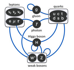
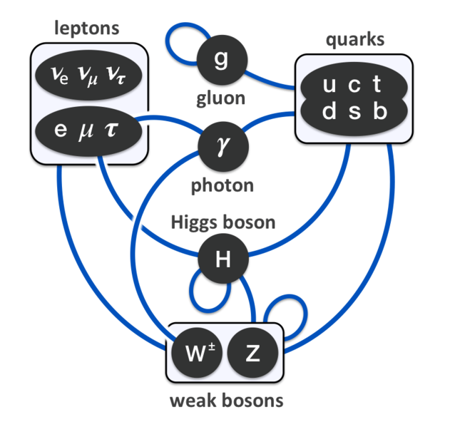
As this blog makes abundantly clear, it’s not easy to ‘summarize’ the Standard Model in a couple of sentences or in one simple diagram. In fact, I’d say that’s impossible. If there’s one or two diagrams sort of ‘covering’ it all, then it’s the two diagrams that you’ve seen ad nauseam already: (a) the overview of the three generations of matter, with the gauge bosons for the electromagnetic, strong and weak force respectively, as well as the Higgs boson, next to it, and (b) the overview of the various interactions between them. [And, yes, these two diagrams come from Wikipedia.]

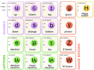
I’ve said it before: the complexity of the Standard Model (it has not less than 61 ‘elementary’ particles taking into account that quarks and gluons come in various ‘colors’, and also including all antiparticles – which we have to include them in out count because they are just as ‘real’ as the particles), and the ‘weirdness’ of the weak force, plus a astonishing range of other ‘particularities’ (these ‘quantum numbers’ or ‘charges’ are really not easy to ‘understand’), do not make for a aesthetically pleasing theory but, let me repeat it again, it’s the best we’ve got. Hence, we may not ‘like’ it but, as Feynman puts it: “Whether we like or don’t like a theory is not the essential question. It is whether or not the theory gives predictions that agree with experiment.” (Feynman, QED – The Strange Theory of Light and Matter, p. 10)

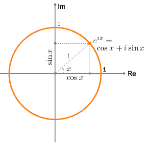
It would be foolish to try to reduce the complexity of the Standard Model to a couple of sentences. That being said, when digging into the subject-matter of quantum mechanics over the past year, I actually got the feeling that, when everything is said and done, modern physics has quite a lot in common with Pythagoras’ ‘simple’ belief that mathematical concepts – and numbers in particular – might have greater ‘actuality’ than the reality they are supposed to describe. To put it crudely, the only ‘update’ to the Pythagorean model that’s needed is to replace Pythagoras’ numerological ideas by the equipartition theorem and quantum-mechanical wave functions, describing probability amplitudes that are represented by complex numbers. Indeed, complex numbers are numbers too, and Pythagoras would have reveled in their beauty. In fact, I can’t help thinking that, if he could have imagined them, he would surely have created a ‘religion’ around Euler’s formula, rather than around the tetrad. 🙂

In any case… Let’s leave the jokes and the silly comparisons aside, as that’s not what I want to write about in this post (if you want to read more about this, I’ll refer you another blog of mine). In this post, I want to present the basics of vector calculus, an understanding of which is absolutely essential in order to gain both a mathematical as well as a ‘physical’ understanding of what fields really are. So that’s classical mechanics once again. However, as I found out, one can’t study quantum mechanics without going through the required prerequisites. So let’s go for it.

Vectors in math and physics

What’s a vector? It may surprise you, but the term ‘vector’, in physics and in math, refers to more than a dozen different concepts, and that’s a major source of confusion for people like us–autodidacts. The term ‘vector’ refers to many different things indeed. The most common definitions are:

The term ‘vector’ often refers to a (one-dimensional) array of numbers. In that case, a vector is, quite simply, an element of Rⁿ, while the array will be referred to as an n-tuple. This definition can be generalized to also include arrays of alphanumerical values, or blob files, or any type of object really, but that’s a definition that’s more relevant for other sciences – most notably computer science. In math and physics, we usually limit ourselves to arrays of numbers. However, you should note that a ‘number’ may also be a complex number, and so we have real as well as complex vector spaces. The most straightforward example of a complex vector space is the set of complex numbers itself: C. In that case, the n-tuple is a ‘1-tuple’, aka as a singleton, but the element in it (i.e. a complex number) will have ‘two dimensions’, so to speak. [Just like the term ‘vector’, the term ‘dimension’ has various definitions in math and physics too, and so it may be quite confusing.] However, we can also have 2-tuples, 3-tuples or, more in general, n-tuples of complex numbers. In that case, the vector space is denoted by Cⁿ. I’ve written about vector spaces before and so I won’t say too much about this.
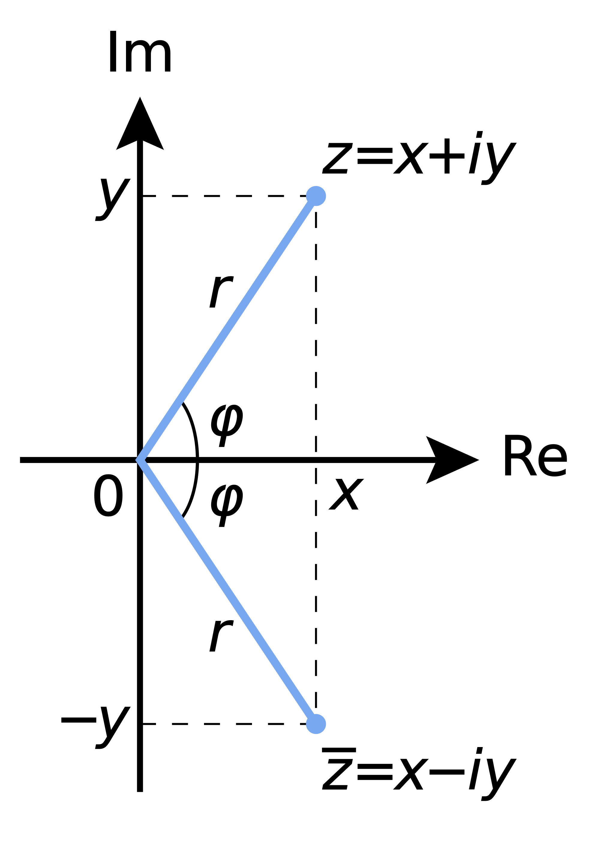
A vector can also be a point vector. In that case, it represents the position of a point in physical space – in one, two or three dimensions – in relation to some arbitrarily chosen origin (i.e. the zero point). As such, we’ll usually write it as x (in one dimension) or, in three dimensions, as (x, y, z). More generally, a point vector is often denoted by the bold-face symbol R. This definition is obviously ‘related’ to the definition above, but it’s not the same: we’re talking physical space here indeed, not some ‘mathematical’ space. Physical space can be curved, as you obviously know when you’re reading this blog, and I also wrote about that in the above-mentioned post, so you can re-visit that topic too if you want. Here, I should just mention one point which may or may not confuse you: while (two-dimensional) point vectors and complex numbers have a lot in common, they are not the same, and it’s important to understand both the similarities as well as the differences between both. For example, multiplying two vectors and multiplying two complex numbers is definitely not the same. I’ll come back to this.
A vector can also be a displacement vector: in that case, it will specify the change in position of a point relative to its previous position. Again, such displacement vectors may be one-, two-, or three-dimensional, depending on the space we’re envisaging, which may be one-dimensional (a simple line), two-dimensional (i.e. the plane), three-dimensional (i.e. three-dimensional space), or four-dimensional (i.e. space-time). A displacement vector is often denoted by s or ΔR, with the delta indicating we’re talking a a distance or a difference indeed: s = ΔR = R₂ – R₁ = (x₂ – x₁, y₂ – y₁, z₂ – z₁). That’s kids’ stuff, isn’t it?
A vector may also refer to a so-called four-vector: a four-vector obeys very specific transformation rules, referred to as the Lorentz transformation. In this regard, you’ve surely heard of space-time vectors, referred to as events, and noted as X = (ct, r), with r the spatial vector r = (x, y, z) and c the speed of light (which, in this case, is nothing but a proportionality constant ensuring that space and time are measured in compatible units). So we can also write X as X = (ct, x, y, z). However, there is another four-vector which you’ve probably also seen already (see, for example, my post on (special) Relativity Theory): P = (E/c, p), which relates energy and momentum in spacetime. Of course, spacetime can also be curved. In fact, Einstein’s (general) Relativity Theory is about the curvature of spacetime, not of ordinary space. But I should not write more about this here, as it’s about time I get back to the main story line of this post.
Finally, we also have vector operators, like the gradient vector ∇. Now that is what I want to write about in this post. Vector operators are also considered to be ‘vectors’ – to some extent, at least: we use them in a ‘vector products’, for example, as I will show below – but, because they are operators and, as such, “hungry for something to operate on”, they are obviously quite different from any of the ‘vectors’ I defined in point (1) to (4) above. [Feynman attributes this ‘hungry for something to operate on’ expression to the British mathematician Sir James Hopwood Jeans, who’s best known from the infamous Rayleigh-Jeans law, whose inconsistency with observations is known as the ultraviolet catastrophe or ‘black-body radiation problem’. But that’s a fairly useless digression so let me got in with it.]

In a text on physics, the term ‘vector’ may refer to any of the above but it’s often the second and third definition (point and/or displacement vectors) that will be implicit. As mentioned above, I want to write about the fifth ‘type’ of vector: vector operators. Now, the title of this post is ‘vector calculus’, and so you’ll immediately wonder why I say these vector operators may or may not be defined as vectors. Moreover, the fact of the matter is that these operators operate on yet another type of ‘vector’ – so that’s a sixth definition I need to introduce here: field vectors.

Now, funnily enough, the term ‘field vector’, while being the most obvious description of what it is, is actually not widely used: what I call a ‘field vector’ is often referred to as a gradient vector, and the vectors E and B are usually referred to as the electric or magnetic field, tout court. Indeed, if you google the terms ‘electromagnetic vector’ (or electric or magnetic vector), you will usually be redirected. However, when everything is said and done, E and B are vectors: they have a magnitude, and they have a direction. To be even more precise, while they depend on both space and time – so we can write E as E = E(x, y, z, t) and we have four independent variables here – they have three components: one of each direction in space, so we can write E as:

E = E(x, y, z, t) = [E_x, E_y, E_z] = [E_x(x, y, z, t), E_y(x, y, z, t), E_z(x, y, z, t)]

So, truth be told, vector calculus (aka vector analysis) in physics is about (vector) fields and (vector) operators,. While the ‘scene’ for these fields and operators is, obviously, physical space (or spacetime) and, hence, a vector space, it’s good to be clear on terminology and remind oneself that, in physics, vector calculus is not about mathematical vectors: it’s about real stuff. That’s why Feynman prefers a much longer term than vector calculus or vector analysis: he calls it differential calculus of vector fields which, indeed, is what it is – but I am sure you would not have bothered starting reading this post if I would have used that term too. 🙂

Now, this has probably become the longest introduction ever to a blog post, and so I had better get on with it. 🙂

Vector fields and scalar fields

Let’s dive straight into it. Vector fields like E and B behave like h, which is the symbol used in a number of textbooks for the heat flow in some body or block of material: E, B and h are all vector fields derived from a scalar field.

Huh? Scalar field? Aren’t we talking vectors? We are. If I say we can derive the vector field h (i.e. the heat flow) from a scalar field, I am basically saying that the relationship between h and the temperature T (i.e. the scalar field) is direct and very straightforward. Likewise, the relationship between E and the scalar field Φ is also direct and very straightforward.

[To be fully precise and complete, I should qualify the latter statement: it’s only true in electrostatics, i.e. when we’re considering charges that don’t move. When we have moving charges, magnetic effects come into play, and then we have a more complicated relationship between (i) two scalar fields, namely A (the magnetic potential – i.e. the ‘magnetic scalar field’) and Φ (the electrostatic potential, or ‘electric scalar field’), and (ii) two vector fields, namely B and E. The relationships between the two are then a bit more complicated than the relationship between T and h. However, the math involved is the same. In fact, the complication arises from the fact that magnetism is actually a relativistic effect. However, at this stage, this statement will only confuse you, and so I will write more about that in my next post.]

Let’s look at h and T. As you know, the temperature is a measure for energy. In a block of material, the temperature T will be a scalar: some real number that we can measure in Kelvin, Fahrenheit or Celsius but – whatever unit we use – any observer using the same unit will measure the same at any given point. That’s what distinguishes a ‘scalar’ quantity from ‘real numbers’ in general: a scalar field is something real. It represents something physical. A real number is just… Well… A real number, i.e. a mathematical concept only.

The same is true for a vector field: it is something real. As Feynman puts it: “It is not true that any three numbers form a vector [in physics]. It is true only if, when we rotate the coordinate system, the components of the vector transform among themselves in the correct way.” What’s the ‘correct way’? It’s a way that ensures that any observer using the same unit will measure the same at any given point.

How does it work?

In physics, we associate a point in space with physical realities, such as:

Temperature, the ‘height‘ of a body in a gravitational field, or the pressure distribution in a gas or a fluid, are all examples of scalar fields: they are just (real) numbers from a math point of view but, because they do represent a physical reality, these ‘numbers’ respect certain mathematical conditions: in practice, they will be a continuous or continuously differentiable function of position.
Heat flow (h), the velocity (v) of the molecules/atoms in a rotating object, or the electric field (E), are examples of vector fields. As mentioned above, the same condition applies: any observer using the same unit should measure the same at any given point.
Tensors, which represent, for example, stress or strain at some point in space (in various directions), or the curvature of space (or spacetime, to be fully correct) in the general theory of relativity.
Finally, there are also spinors, which are often defined as a “generalization of tensors using complex numbers instead of real numbers.” They are very relevant in quantum mechanics, it is said, but I don’t know enough about them to write about them, and so I won’t.

How do we derive a vector field, like h, from a scalar field (i.e. T in this case)? The two illustrations below (taken from Feynman’s Lectures) illustrate the ‘mechanics’ behind it: heat flows, obviously, from the hotter to the colder places. At this point, we need some definitions. Let’s start with the definition of the heat flow: the (magnitude of the) heat flow (h) is the amount of thermal energy (ΔJ) that passes, per unit time and per unit area, through an infinitesimal surface element at right angles to the direction of flow.

A vector has both a magnitude and a direction, as defined above, and, hence, if we define e_f as the unit vector in the direction of flow, we can write:

h = h·e_f = (ΔJ/Δa)·e_f

ΔJ stands for the thermal energy flowing through an area marked as Δa in the diagram above per unit time. So, if we incorporate the idea that the aspect of time is already taken care of, we can simplify the definition above, and just say that the heat flow is the flow of thermal energy per unit area. Simple trigonometry will then yield an equally simple formula for the heat flow through any surface Δa₂ (i.e. any surface that is not at right angles to the heat flow h):

ΔJ/Δa₂ = (ΔJ/Δa₁)cosθ = h·n

When I say ‘simple’, I must add that all is relative, of course, Frankly, I myself did not immediately understand why the heat flow through the Δa₁ and Δa₂ areas below must be the same. That’s why I added the blue square in the illustration above (which I took from Feynman’s Lectures): it’s the same area as Δa₁, but it shows more clearly – I hope! – why the heat flow through the two areas is the same indeed, especially in light of the fact that we are looking at infinitesimally small areas here (so we’re taking a limit here).

As for the cosine factor in the formula above, you should note that, in that ΔJ/Δa₂ = (ΔJ/Δa₁)cosθ = h·n equation, we have a dot product (aka as a scalar product) of two vectors: (1) h, the heat flow and (2) n, the unit vector that is normal (orthogonal) to the surface Δa₂. So let me remind you of the definition of the scalar (or dot) product of two vectors. It yields a (real) number:

A·B = |A||B|cosθ, with θ the angle between A and B

In this case, h·n = |h||n|cosθ = |h|·1·cosθ = |h|cosθ = h·cosθ. What we are saying here is that we get the component of the heat flow that’s perpendicular (or normal, as physicists and mathematicians seem to prefer to say) to the surface Δa₂ by taking the dot product of the heat flow h and the unit normal n. We’ll use this formula later, and so it’s good to take note of it here.

OK. Let’s get back to the lesson. The only thing that we need to do to prove that ΔJ/Δa₂ = (ΔJ/Δa₁)cosθ formula is show that Δa₂ = Δa₁/cosθ or, what amounts to the same, that Δa₁ = Δa₂cosθ. Now that is something you should be able to figure out yourself: it’s quite easy to show that the angle between h and n is equal to the angle between the surfaces Δa₁ and Δa₂. The rest is just plain triangle trigonometry.

For example, when the surfaces coincide, the angle θ will be zero and then h·n is just equal to |h|cosθ = |h| = h·1 = h = ΔJ/Δa₁. The other extreme is that orthogonal surfaces: in that case, the angle θ will be 90° and, hence, h·n = |h||n|cos(π/2) = |h|·1·0 = 0: there is no heat flow normal to the direction of heat flow.

OK. That’s clear enough. The point to note is that the vectors h and n represent physical entities and, therefore, they do not depend on our reference frame (except for the units we use to measure things). That allows us to define vector equations.

The ∇ (del) operator and the gradient

Let’s continue our example of temperature and heat flow. In a block of material, the temperature (T) will vary in the x, y and z direction and, hence, the partial derivatives ∂T/∂x, ∂T/∂y and ∂T/∂z make sense: they measure how the temperature varies with respect to position. Now, the remarkable thing is that the 3-tuple (∂T/∂x, ∂T/∂y, ∂T/∂z) is a physical vector itself: it is independent, indeed, of the reference frame (provided we measure stuff in the same unit) – so we can do a translation and/or a rotation of the coordinate axes and we get the same value. This means this set of three numbers is a vector indeed:

(∂T/∂x, ∂T/∂y, ∂T/∂z) = a vector

If you like to see a formal proof of this, I’ll refer you to Feynman once again – but I think the intuitive argument will do: if temperature and space are real, then the derivatives of temperature in regard to the x-, y- and z-directions should be equally real, isn’t it? Let’s go for the more intricate stuff now.

If we go from one point to another, in the x-, y- or z-direction, then we can define some (infinitesimally small) displacement vector ΔR = (Δx, Δy, Δz), and the difference in temperature between two nearby points (ΔT) will tend to the (total) differential of T – which we denote by ΔT – as the two point get closer and closer. Hence, we write:

ΔT = (∂T/∂x)Δx + (∂T/∂y)Δy + (∂T/∂z)Δz

The two equations above combine to yield:

ΔT = (∂T/∂x, ∂T/∂y, ∂T/∂z)(Δx, Δy, Δz) = ∇T·ΔR

In this equation, we used the ∇ (del) operator, i.e. the vector differential operator. It’s an operator like the differential operator ∂/∂x (i.e. the derivative) but, unlike the derivative, it returns not one but three values, i.e. a vector, which is usually referred to as the gradient, i.e. ∇T in this case. More in general, we can write ∇f(x, y, z), ∇ψ or ∇ followed by whatever symbol for the function we’re looking at.

In other words, the ∇ operator acts on a scalar-valued function (T), aka a scalar field, and yields a vector:

∇T = (∂T/∂x, ∂T/∂y, ∂T/∂z)

That’s why we write ∇ in bold-type too, just like the vector R. Indeed, using bold-type (instead of an arrow or so) is a convenient way to mark a vector, and the difference (in print) between ∇ and ∇ is subtle, but it’s there – and for a good reason as you can see!

[To be precise, I should add that we do not write all of the operators that return three components in bold-type. The most simple example is the common derivative ∂E/∂t = [∂E_x/∂t, ∂E_y/∂t, ∂E_z/∂t]. We have a lot of other possible combinations. Some make sense, and some don’t, like ∂h/∂y = [∂h_x/∂y, ∂h_y/∂y, ∂h_z/∂y], for example.]

If ∇T is a vector, what’s its direction? Think about it. […] The rate of change of T in the x-, y- and z-direction are the x-, y- and z-component of our ∇T vector respectively. In fact, the rate of change of T in any direction will be the component of the ∇T vector in that direction. Now, the magnitude of a vector component will always be smaller than the magnitude of the vector itself, except if it’s the component in the same direction as the vector, in which case the component is the vector. [If you have difficulty understanding this, read what I write once again, but very slowly and attentively.] Therefore, the direction of ∇T will be the direction in which the (instantaneous) rate of change of T is largest. In Feynman’s words: “The gradient of T has the direction of the steepest uphill slope in T.” Now, it should be quite obvious what direction that really is: it is the opposite direction of the heat flow h.

That’s all you need to know to understand our first real vector equation:

h = –κ∇T

Indeed, you don’t need too much math to understand this equation in the way we want to understand it, and that’s in some kind of ‘physical‘ way (as opposed to just the math side of it). Let me spell it out:

The direction of heat flow is opposite to the direction of the gradient vector ∇T. Hence, heat flows from higher to lower temperature (i.e. ‘downhill’), as we would expect, of course!). So that’s the minus sign.
The magnitude of h is proportional to the magnitude of the gradient ∇T, with the constant of proportionality equal to κ (kappa), which is called the thermal conductivity. Now, in case you wonder what this means (again: do go beyond the math, please!), remember that the heat flow is the flow of thermal energy per unit area (and per unit time, of course): |h| = h = ΔJ/Δa.

But… Yes? Why would it be proportional? Why don’t we have some exponential relation or something? Good question, but the answer is simple, and it’s rooted in physical reality – of course! The heat flow between two places – let’s call them 1 and 2 – is proportional to the temperature difference between those two places, so we have: ΔJ ∼ T₂ – T₁. In fact, that’s where the factor of proportionality comes in. If we imagine a very small slab of material (infinitesimally small, in fact) with two faces, parallel to the isothermals, with a surface area ΔA and a tiny distance Δs between them, we can write:

ΔJ = κ(T₂ – T₁)ΔA/Δs = ΔJ = κ·ΔT·ΔA/Δs ⇔ ΔJ/ΔA = κΔT/Δs

Now, we defined ΔJ/ΔA as the magnitude of h. As for its direction, it’s obviously perpendicular (not parallel) to the isothermals. Now, as Δs tends to zero, ΔT/Δs is nothing but the rate of change of T with position. We know it’s the maximum rate of change, because the position change is also perpendicular to the isotherms (if the faces are parallel, that tiny distance Δs is perpendicular). Hence, ΔT/Δs must be the magnitude of the gradient vector (∇T). As its direction is opposite to that of h, we can simply pop in a minus sign and switch from magnitudes to vectors to write what we wrote already: h = –κ∇T.

But let’s get back to the lesson. I think you ‘get’ all of the above. In fact, I should probably not have introduced that extra equation above (the ΔJ expression) and all the extra stuff (i.e. the ‘infinitesimally small slab’ explanation), as it probably only confuses you. So… What’s the point really? Well… Let’s look, once again, at that equation h = –κ∇T and let us generalize the result:

We have a scalar field here, the temperature T – but it could be any scalar field really!
When we have the ‘formula’ for the scalar field – it’s obviously some function T(x, y, z) – we can derive the heat flow h from it, i.e. a vector quantity, which has a property which we can vaguely refer to as ‘flow’.
We do so using this brand-new operator ∇. That’s a so-called vector differential operator aka the del operator. We just apply it to the scalar field and we’re done! The only thing left is to add some proportionality factor, but so that’s just because of our units. [In case you wonder about the symbol it self, ∇ is the so-called nabla symbol: the name comes from the Hebrew word for a harp, which has a similar shape indeed.]

This truly is a most remarkable result, and we’ll encounter the same equation elsewhere. For example, if the electric potential is Φ, then we can immediately calculate the electric field using the following formula:

E = –∇Φ

Indeed, the situation is entirely analogous from a mathematical point of view. For example, we have the same minus sign, so E also ‘flows’ from higher to lower potential. Where’s the factor of proportionality? Well… We don’t have one, as we assume that the units in which we measure E and Φ are ‘fully compatible’ (so don’t worry about them now). Of course, as mentioned above, this formula for E is only valid in electrostatics, i.e. when there are no moving charges. When moving charges are involved, we also have the magnetic force coming into play, and then equations become a bit more complicated. However, this extra complication does not fundamentally alter the logic involved, and I’ll come back to this so you see how it all nicely fits together.

Note: In case you feel I’ve skipped some of the ‘explanation’ of that vector equation h = –κ∇T… Well… You may be right. I feel that it’s enough to simply point out that ∇T is a vector with opposite direction to h, so that explains the minus sign in front of the ∇T factor. The only thing left to ‘explain’ then is the magnitude of h, but so that’s why we pop in that kappa factor (κ), and so we’re done, I think, in terms of ‘understanding’ this equation. But so that’s what I think indeed. Feynman offers a much more elaborate ‘explanation‘, and so you can check that out if you think my approach to it is a bit too much of a shortcut.

Interim summary

So far, we have only have shown two things really:

[I] The first thing to always remember is that h·n product: it gives us the component of ‘flow’ (per unit time and per unit area) of h perpendicular through any surface element Δa. Of course, this result is valid for any other vector field, or any vector for that matter: the scalar product of a vector and a unit vector will always yield the component of that vector in the direction of that unit vector. [But note the second vector needs to be a unit vector: it is not generally true that the dot product of one vector with another yields the component of the first vector in the direction of the second: there’s a scale factor that comes into play.]

Now, you should note that the term ‘component’ (of a vector) usually refers to a number (not to a vector) – and surely in this case, because we calculate it using a scalar product! I am just highlighting this because it did confuse me for quite a while. Why? Well… The concept of a ‘component’ of a vector is, obviously, intimately associated with the idea of ‘direction’: we always talk about the component in some direction, e.g. in the x-, y- or z-direction, or in the direction of any combination of x, y and z. Hence, I think it’s only natural to think of a ‘component’ as a vector in its own right. However, as I note here, we shouldn’t do that: a ‘component’ is just a magnitude, i.e. a number only. If we’d want to include the idea of direction, it’s simple: we can just multiply the component with the normal vector n once again, and then we have a vector quantity once again, instead of just a scalar. So then we just write (h·n)·n = (h·n)n. Simple, isn’t it? 🙂

[As I am smiling here, I should quickly say something about this dot (·) symbol: we use the same symbol here for (i) a product between scalars (i.e. real or complex numbers), like 3·4; (ii) a product between a scalar and a vector, like 3·v – but then I often omit the dot to simply write 3v; and, finally, (iii) a scalar product of two vectors, like h·n indeed. We should, perhaps, introduce some new symbol for multiplying numbers, like ∗ for example, but then I hope you’re smart enough to see from the context what’s going on really.]

Back to the lesson. Let me jot down the formula once again: h·n = |h||n|cosθ = h·cosθ. Hence, the number we get here is h (i.e. the amount of heat flow in the direction of flow) multiplied by cosθ, with θ the angle between (i) the surface we’re looking at (which, as mentioned above, is any surface really) and (ii) the surface that’s perpendicular to the direction of flow.

Hmm… […] The direction of flow? Let’s take a moment to think about what we’re saying here. Is there any particular or unique direction really? Heat flows in all directions from warmer to colder areas, and not just in one direction, doesn’t it? You’re right. Once again, the terminology may confuse you – which is yet another reason why math is so much better as a language to express physical ideas 🙂 – and so we should be precise: the direction of h is the direction in which the amount of heat flow (i.e. h·cosθ) is largest (hence, the angle θ is zero). As we pointed out above, that’s the direction in which the temperature T changes the fastest. In fact, as Feynman notes: “We can, if we wish, consider that this statement defines h.”

That brings me to the second thing you should – always and immediately – remember from all of that I’ve written above.

[II] If we write the infinitesimal (i.e. the differential) change in temperature (in whatever direction) as ΔT, then we know that

ΔT = (∂T/∂x, ∂T/∂y, ∂T/∂z)(Δx, Δy, Δz) = ∇T·ΔR

Now, what does this say really? ΔR is an (infinitesimal) displacement vector: ΔR = (Δx, Δy, Δz). Hence, it has some direction. To be clear: that can be any direction in space really. So that’s simple. What about the second factor in this dot product, i.e. that gradient vector ∇T?

The direction of the gradient (i.e. ∇T) is not just ‘any direction’: it’s the direction in which the rate of change of T is largest, and we know what direction that is: it’s the opposite direction of the heat flow h, as evidenced by the minus sign in our vector equations h = –κ∇T or E = –∇Φ. So, once again, we have a (scalar) product of two vectors here, ∇T·ΔR, which yields… Hmm… Good question. That ∇T·ΔR expression is very similar to that h·n expression above, but it’s not quite the same. It’s also a vector dot product – or a scalar product, in other words, but, unlike that n vector, the ΔR vector is not a unit vector: it’s an infinitesimally small displacement vector. So we do not get some ‘component’ of ∇T. More in general, you should note that the dot product of two vectors A and B does not, in general, yield the component of A in the direction of B, unless B is a unit vector – which, again, is not the case here. So if we don’t have that here, what do we have?

Let’s look at the (physical) geometry of the situation once again. Heat obviously flows in one direction only: from warmer to colder places – not in the opposite direction. Therefore, the θ in the h·n = h·cosθ expression varies from –90° to +90° only. Hence, the cosine factor (cosθ) is always positive. Always. Indeed, we do not have any right- or left-hand rule here to distinguish between the ‘front’ side and the ‘back’ side of our surface area. So when we’re looking at that h·n product, we should remember that that normal unit vector n is a unit vector that’s normal to the surface but which is oriented, generally, towards the direction of flow. Therefore, that h·n product will always yield some positive value, because θ varies from –90° to +90° only indeed.

When looking at that ΔT = ∇T·ΔR product, the situation is quite different: while ∇T has a very specific direction (I really mean unique) – which, as mentioned above is opposite to that of h – that ΔR vector can point in any direction – and then I mean literally any direction, including directions ‘uphill’. Likewise, it’s obvious that the temperature difference ΔT can be both positive or negative (or zero, when we’re moving on a isotherm itself). In fact, it’s rather obvious that, if we go in the direction of flow, we go from higher to lower temperatures and, hence, ΔT will, effectively, be negative: ΔT = T₂ – T₁ < 0, as shown below.

Now, because |∇T| and |ΔR| are absolute values (or magnitudes) of vectors, they are always positive (always!). Therefore, if ΔT has a minus sign, it will have to come from the cosine factor in the ΔT = ∇T·ΔR = |∇T|·|ΔR|·cosθ expression. [Again, if you wonder where this expression comes from: it’s just the definition of a vector dot product.] Therefore, ΔT and cosθ will have the same sign, always, and θ can have any value between –180° to +180°. In other words, we’re effectively looking at the full circle here. To make a long story short, we can write the following:

ΔT = |∇T|·|ΔR|·cosθ = |∇T|·ΔR·cosθ ⇔ ΔT/ΔR = |∇T|cosθ

As you can see, θ is the angle between ∇T and ΔR here and, as mentioned above, it can take on any value – well… Any value between –180° to +180°, that is. ΔT/ΔR is, obviously, the rate of change of T in the direction of ΔR and, from the expression above, we can see it is equal to the component of ∇T in the direction of ΔR:

ΔT/ΔR = |∇T|cosθ

So we have a negative component here? Yes. The rate of change is negative and, therefore, we have a negative component. Indeed, any vector has components in all directions, including directions that point away from it. However, in the directions that point away from it, the component will be negative. More in general, we have the following interesting result: the rate of change of a scalar field ψ in the direction of a (small) displacement ΔR is the component of the gradient ∇ψ along that displacement. We write that result as:

Δψ/ΔR = |∇ψ|cosθ

[Note the (not so) subtle difference between ΔR (i.e. a vector) and ΔR (some real number). It’s quite important. ]

We’ve said a lot of (not so) interesting things here, but we still haven’t answered the original question: what’s ∇T·ΔR? Well… We can’t say more than what we said already: it’s equal to ΔT, which is a differential: ΔT = (∂T/∂x)Δx + (∂T/∂y)Δy + (∂T/∂z)Δz. A differential and a derivative (i.e. a rate of change) are not the same, but they are obviously closely related, as evidenced from the equations above: the rate of change is the change per unit distance. [Likewise, note that |∇ψ|cosθ is just a product of two real numbers, while ∇T·ΔR is a vector dot product, i.e. a (scalar) product of two vectors!]

In any case, this is enough of a recapitulation. In fact, this ‘interim summary’ has become longer than the preceding text! We’re now ready to discuss what I’ll call the First Theorem of vector calculus in physics. Of course, never mind the term: what’s first or second or third doesn’t matter really: you’ll need all of the theorems below to understand vector calculus.

The First Theorem

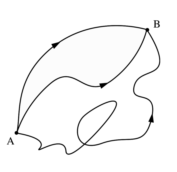
Let’s assume we have some scalar field ψ in space: ψ might be the temperature, but it could be any scalar field really. Now, if we go from one point (1) to another (2) in space, as shown below, we’ll follow some arbitrary path, which is denoted by the curve Γ in the illustrations below. Each point along the curve can then be associated with a gradient ∇ψ (think of the h = –κ∇T and E = –∇Φ expressions above if you’d want examples). Its tangential component is obviously equal to (∇ψ)_t·Δs= ∇ψ·Δs. [Please note, once again, the subtle difference between Δs(with the s in bold-face) and Δs: Δsis a vector, and Δsis its magnitude.]

As shown in the illustrations above, we can mark off the curve at a number of points (a, b, c, etcetera) and join these points by straight-line segments Δs_i. Now let’s consider the first line segment, i.e. Δs₁. It’s obvious that the change in ψ from point 1 to point a is equal to Δψ₁= ψ(a) – ψ(1). Now, we have that general Δψ = (∂ψ/∂x, ∂ψ/∂y, ∂ψ/∂z)(Δx, Δy, Δz) = ∇ψ·Δs equation. [If you find it difficult to interpret what I am writing here, just substitute ψ for T and Δs for ΔR.] So we can write:

Δψ₁= ψ(a) – ψ(1) = (∇ψ)₁·Δs₁

Likewise, we can write:

ψ(b) – ψ(a) = (∇ψ)₂·Δs₁

In these expressions, (∇ψ)₁and (∇ψ)₂mean the gradient evaluated at segment Δs₁ and point Δs₂ respectively, not at point 1 and 2 – obviously. Now, if we add the two equations above, we get:

ψ(b) – ψ(1) = (∇ψ)₁·Δs₁+ (∇ψ)₂·Δs₁

To make a long story short, we can keep adding such terms to get:

ψ(2) – ψ(1) = ∑(∇ψ)_i·Δs_i

We can add more and more segments and, hence, take a limit: as Δs_i tends to zero, ∑ becomes a sum of an infinite number of terms – which we denote using the integral sign ∫ – in which ds is – quite simply – just the infinitesimally small displacement vector. In other words, we get the following line integral along that curve Γ:

This is a gem, and our First Theorem indeed. It’s a remarkable result, especially taking into account the fact that the path doesn’t matter: we could have chosen any curve Γ indeed, and the result would be the same. So we have:

You’ll say: so what? What do we do with this? Well… Nothing much for the moment, but we’ll need this result later. So I’d say: just hang in there, and note this is the first significant use of our del operator in a mathematical expression that you’ll encounter very often in physics. So just let it sink in, and allow me to proceed with the rest of the story.

Before doing so, however, I should note that even Feynman sins when trying to explain this theorem in a more ‘intuitive’ way. Indeed, in his Lecture on the topic, he writes the following: “Since the gradient represents the rate of change of a field quantity, if we integrate that rate of change, we should get the total change.” Now, from that Δψ/ΔR = |∇ψ|cosθ formula, it’s obvious that the gradient is the rate of change in a specific direction only. To be precise, in this particular case – with the field quantity ψ equal to the temperature T – it’s the direction in which T changes the fastest.

You should also note that the integral above is not the type of integral you known from high school. Indeed, it’s not of the rather straightforward ∫f(x)dx type, with f(x) the integrand and dx the variable of integration. That type of integral, we knew how to solve. A line integral is quite different. Look at it carefully: we have a vector dot product after the ∫ sign. So, unlike what Feynman suggests, it’s not just a matter of “integrating the rate of change.”

Now, I’ll refer you to Wikipedia for a good discussion of what a line integral really is, but I can’t resist the temptation to copy the animation in that article, because it’s very well made indeed. While it shows that we can think of a line integral as the two- or three-dimensional equivalent of the standard type of integral we learned to solve in high school (you’ll remember the solution was also the area under the graph of the function that had to be integrated), the way to go about it is quite different. Solving them will, in general, involve some so-called parametrization of the curve C.

However, this post is becoming way too long and, hence, I really need to move on now.

Operations with ∇: divergence and curl

You may think we’ve covered a lot of ground already, and we did. At the same time, everything I wrote above is actually just the start of it. I emphasized the physics of the situation so far. Let me now turn to the math involved. Let’s start by dissociating the del operator from the scalar field, so we just write:

∇ = (∂/∂x, ∂/∂y, ∂/∂z)

This doesn’t mean anything, you’ll say, because the operator has nothing to operate on. And, yes, you’re right. However, in math, it doesn’t matter: we can combine this ‘meaningless’ operator (which looks like a vector, because it has three components) with something else. For example, we can do a vector dot product:

∇·(a vector)

As mentioned above, we can ‘do’ this product because ∇ has three components, so it’s a ‘vector’ too (although I find such name-giving quite confusing), and so we just need to make sure that the vector we’re operating on has three components too. To continue with our heat flow example, we can write, for example:

∇·h = (∂/∂x, ∂/∂y, ∂/∂z)·(h_x, h_y, h_z) = ∂h_x/∂x + ∂h_y/∂y, ∂h_z/∂z

This del operator followed by a dot, and acting on a vector – i.e. ∇·(vector) – is, in fact, a new operator. Note that we use two existing symbols, the del (∇) and the dot (·), but it’s one operator really. [Inventing a new symbol for it would not be wise, because we’d forget where it comes from and, hence, probably scratch our head when we’d see it.] It’s referred to as a vector operator, just like the del operator, but don’t worry about the terminology here because, once again, the terminology here might confuse you. Indeed, our del operator acted on a scalar to yield a vector, and now it’s the other way around: we have an operator acting on a vector to return a scalar. In a few minutes, we’ll define yet another operator acting on a vector to return a vector. Now, all of these operators are so-called vector operators, not because there’s some vector involved, but because they all involve the del operator. It’s that simple. So there’s no such thing as a scalar operator. 🙂 But let me get back to the main line of the story. This ∇· operator is quite important in physics, and so it has a name (and an abbreviated notation) of its own:

∇·h = div h = the divergence of h

The physical significance of the divergence is related to the so-called flux of a vector field: it measures the magnitude of a field’s source or sink at a given point. Continuing our example with temperature, consider air as it is heated or cooled. The relevant vector field is now the velocity of the moving air at a point. If air is heated in a particular region, it will expand in all directions such that the velocity field points outward from that region. Therefore the divergence of the velocity field in that region would have a positive value, as the region is a source. If the air cools and contracts, the divergence has a negative value, as the region is a sink.

A less intuitive but more accurate definition is the following: the divergence represents the volume density of the outward flux of a vector field from an infinitesimal volume around a given point.

Phew! That sounds more serious, doesn’t it? We’ll come back to this definition when we’re ready to define the concept of flux somewhat accurately. For now, just note two of Maxwell’s famous equations involve the divergence operator:

∇·E = ρ/ε₀ and ∇·B = 0

In my previous post, I gave a verbal description of those two equations:

The flux of E through a closed surface = (the net charge inside)/ε₀
The flux of B through a closed surface = zero

The first equation basically says that electric charges cause an electric field. The second equation basically says there is no such thing as a magnetic charge: the magnetic force only appears when charges are moving and/or when electric fields are changing. Note that we’re talking closed surface here, so they define a volume indeed. We can also look at the flux through a non-closed surface (and we’ll do that shortly) but, in the context of Maxwell’s equations, we’re talking volumes and, hence, closed surfaces.

Let me quickly throw in some remarks on the units in which we measure stuff. Electric field strength (so the unit we use to measure the magnitude of E) is measured in Newton per Coulomb, so force divided by charge. That makes sense, because E is defined as the force on the unit charge: E = F/q, and so the unit is N/C. Please do think about why we have q in the denominator: if we’d have the same force on an electric charge that is twice as big, then we’d have a field strength that’s only half, so we have an inverse proportionality here. Conversely, if we’d have twice the force on the same electric charge, the field strength would also double.

Now, flux and field strength are obviously related, but not the same. The flux is obviously proportional to the field strength (expressed in N/C), but then we also know it’s some number expressed per unit area. Hence, you might think that the unit of flux is field strength per square meter, i.e. N/C/m². It’s not. It’s a stupid mistake, but one that is commonly made. Flux is expressed in N/C times m², so that’s the product (N/C)·m²= (N·m/C)·m= (J/C)·m. Why is that? Think about the common graphical representation of a field: we just draw lines, all tangent to the direction of the field vector at every point, and the density of the lines (i.e. the number of lines per unit area) represents the magnitude of our electric field vector. Now, the flux through some area is the number of lines we count in that area. Hence, if you double the area, you should get twice the flux. Halve the area, and you should get half the flux. So we have a direct proportionality here. In fact, assuming the electric field is uniform, we can write the (electric) flux as the product of the field strength E and the (vector) area S, so we write Φ_E = E·S = E·S·cosθ.

Huh? Yes. The origin of the mistake is that we, somehow, think the ‘per unit area’ qualification comes with the flux. It doesn’t: it’s in the idea of field strength itself. Indeed, an alternative to the presentation above is just to draw arrows representing the same field strength, as illustrated below. However, instead of drawing more arrows (of some standard length) to represent increasing field strength, we’d just draw longer arrows—not more of them. So then the idea of the number of lines per unit area is no longer valid.

[…] OK. I realize I am probably just confusing you here. Just one more thing, perhaps. We also have magnetic flux, denoted as Φ_B, and it’s defined in the same way: Φ_B = B·S = B·S·cosθ. However, because the unit of magnetic field strength is different, the unit of magnetic flux is different too. It’s the weber, and I’ll let you look up its definition yourself. 🙂 Note that it’s a bit of a different beast, because the magnetic force is a bit of a different beast. 🙂

So let’s get back to our operators. You’ll anticipate the second new operator now, because that’s the one that appears in the other two equations in Maxwell’s set of equations. It’s the cross product:

∇×E = (∂/∂x, ∂/∂y, ∂/∂z)×(E_x, E_y, E_z) = … What?

Well… The cross product is not as straightforward to write down as the dot product. We get a vector indeed, not a scalar, and its three components are:

(∇×E)_z = ∇_xE_y– ∇_yE_x= ∂E_y/∂x – ∂E_x/∂y

(∇×E)_x = ∇_yE_z– ∇_zE_y= ∂E_z/∂y – ∂E_y/∂z

(∇×E)_y = ∇_zE_x– ∇_xE_z= ∂E_x/∂z – ∂E_z/∂x

I know this looks pretty monstrous, but so that’s how cross products work. Please do check it out: you have to play with the order of the x, y and z subscripts. I gave the geometric formula for a dot product above, so I should also give you the same for a cross product:

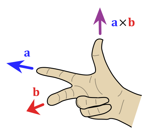
A×B = |A||B|sin(θ)n

In this formula, we once again have θ, the angle between A and B, but note that, this time around, it’s the sine, not the cosine, that pops up when calculating the magnitude of this vector. In addition, we have n at the end: n is a unit vector at right angles to both A and B. It’s what makes the cross product a vector. Indeed, as you can see, multiplying by n will not alter the magnitude (|A||B|sinθ) of this product, but it gives the whole thing a direction, so we get a new vector indeed. Of course, we have two unit vectors at right angles to A and B, and so we need a rule to choose one of these: the direction of the n vector we want is given by that right-hand rule which we encountered a couple of times already.

Again, it’s two symbols but one operator really, and we also have a special name (and notation) for it:

∇×h = curl h = the curl of h

The curl is, just like the divergence, a so-called vector operator but, as mentioned above, that’s just because it involves the del operator. Just note that it acts on a vector and that its result is a vector too. What’s the geometric interpretation of the curl? Well… It’s a bit hard to describe that but let’s try. The curl describes the ‘rotation’ or ‘circulation’ of a vector field:

The direction of the curl is the axis of rotation, as determined by the right-hand rule.
The magnitude of the curl is the magnitude of rotation.

I know. This is pretty abstract, and I’ll probably have to come back to it in another post. Let’s first ask some basic question: should we associate some unit with the curl? In fact, when you google, you’ll find lots of units used in electromagnetic theory (like the weber, for example), but nothing for circulation. I am not sure why, because if flux is related to some density, the idea of curl (or circulation) is pretty much the same. It’s just that it isn’t used much in actual engineering problems, and surely not those you may have encountered in your high school physics course!

In any case, just note we defined three new operators in this ‘introduction’ to vector calculus:

∇T = grad T = a vector
∇·h = div h = a scalar
∇×h = curl h = a vector

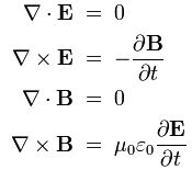
That’s all. It’s all we need to understand Maxwell’s famous equations:

Huh? Hmm… You’re right: understanding the symbols, to some extent, doesn’t mean we ‘understand’ these equations. What does it mean to ‘understand’ an equation? Let me quote Feynman on that: “What it means really to understand an equation—that is, in more than a strictly mathematical sense—was described by Dirac. He said: “I understand what an equation means if I have a way of figuring out the characteristics of its solution without actually solving it.” So if we have a way of knowing what should happen in given circumstances without actually solving the equations, then we “understand” the equations, as applied to these circumstances.”

We’re surely not there yet. In fact, I doubt we’ll ever reach Dirac’s understanding of Maxwell’s equations. But let’s do what we can.

In order to ‘understand’ the equations above in a more ‘physical’ way, let’s explore the concepts of divergence and curl somewhat more. We said the divergence was related to the ‘flux’ of a vector field, and the curl was related to its ‘circulation’. In my previous post, I had already illustrated those two concepts copying the following diagrams from Feynman’s Lectures:

flux = (average normal component)·(surface area)

So that’s the flux (through a non-closed surface).

To illustrate the concept of circulation, we have not one but three diagrams, shown below. Diagram (a) gives us the vector field, such as the velocity field in a liquid. In diagram (b), we imagine a tube (of uniform cross section) that follows some arbitrary closed curve. Finally, in diagram (c), we imagine we’d suddenly freeze the liquid everywhere except inside the tube. Then the liquid in the tube would circulate as shown in (c), and so that’s the concept of circulation.

We have a similar formula as for the flux:

circulation = (the average tangential component)·(the distance around)

In both formulas (flux and circulation), we have a product of two scalars: (i) the average normal component and the average tangential component (for the flux and circulation respectively) and (ii) the surface area and the distance around (again, for the flux and circulation respectively). So we get a scalar as a result. Does that make sense? When we related the concept of flux to the divergence of a vector field, we said that the flux would have a positive value if the region is a source, and a negative value if the region is a sink. So we have a number here (otherwise we wouldn’t be talking ‘positive’ or ‘negative’ values). So that’s OK. But are we talking about the same number? Yes. I’ll show they are the same in a few minutes.

But what about circulation? When we related the concept of circulation of the curl of a vector field, we introduced a vector cross product, so that yields a vector, not a scalar. So what’s the relation between that vector and the number we get when multiplying the ‘average tangential component’ and the ‘distance around’. The answer requires some more mathematical analysis, and I’ll give you what you need in a minute. Let me first make a remark about conventions here.

From what I write above, you see that we use a plus or minus sign for the flux to indicate the direction of flow: the flux has a positive value if the region is a source, and a negative value if the region is a sink. Now, why don’t we do the same for circulation? We said the curl is a vector, and its direction is the axis of rotation as determined by the right-hand rule. Why do we need a vector here? Why can’t we have a scalar taking on positive or negative values, just like we do for the flux?

The intuitive answer to this question (i.e. the ‘non-mathematical’ or ‘physical’ explanation, I’d say) is the following. Although we can calculate the flux through a non-closed surface, from a mathematical point of view, flux is effectively being defined by referring to the infinitesimal volume around some point and, therefore, we can easily, and unambiguously, determine whether we’re inside or outside of that volume. Therefore, the concepts of positive and negative values make sense, as we can define them referring to some unique reference point, which is either inside or outside of the region.

When talking circulation, however, we’re talking about some curve in space. Now it’s not so easy to find some unique reference point. We may say that we are looking at some curve from some point ‘in front of’ that curve, but some other person whose position, from our point of view, would be ‘behind’ the curve, would not agree with our definition of ‘in front of’: in fact, his definition would be exactly the opposite of ours. In short, because of the geometry of the situation involved, our convention in regard to the ‘sign’ of circulation (positive or negative) becomes somewhat more complicated. It’s no longer a simple matter of ‘inward’ or ‘outward’ flow: we need something like a ‘right-hand rule’ indeed. [We could, of course, also adopt a left-hand rule but, by now, you know that, in physics, there’s not much use for a left hand. :-)]

That also ‘explains’ why the vector cross product is non-commutative: A×B ≠ B×A. To be fully precise, A×B and B×A have the same magnitude but opposite direction: A×B = |A||B|sin(θ)n = –|A||B|sin(θ)(–n) = –(B×A) = –B×A. The dot product, on the other hand, is fully commutative: A·B = B·A.

In fact, the concept of circulation is very much related to the concept of angular momentum which, as you’ll remember from a previous post, also involves a vector cross product.

[…]

I’ve confused you too much already. The only way out is the full mathematical treatment. So let’s go for that.

Flux

Some of the confusion as to what flux actually means in electromagnetism is probably caused by the fact that the illustration above is not a closed surface and, from my previous post, you should remember that Maxwell’s first and third equation define the flux of E and B through closed surfaces. It’s not that the formula above for the flux through a non-closed surface is wrong: it’s just that, in electromagnetism, we usually talk about the flux through a closed surface.

A closed surface has no boundary. In contrast, the surface area above does have a clear boundary and, hence, it’s not a closed surface. A sphere is an example of a closed surface. A cube is an example as well. In fact, an infinitesimally small cube is what’s used to prove a very convenient theorem, referred to as Gauss’ Theorem. We will not prove it here, but just try to make sure you ‘understand’ what it says.

Suppose we have some vector field C and that we have some closed surface S – a sphere, for example, but it may also be some very irregular volume. Its shape doesn’t matter: the only requirement is that it’s defined by a closed surface. Let’s then denote the volume that’s enclosed by this surface by V. Now, the flux through some (infinitesimal) surface element da will, effectively, be given by that formula above:

flux = (average normal component)·(surface area)

What’s the average normal component in this case? It’s given by that ΔJ/Δa₂ = (ΔJ/Δa₁)cosθ = h·n formula, except that we just need to substitute h for C here, so we have C·n instead of h·n. To get the flux through the closed surface S, we just need to add all the contributions. Adding those contributions amounts to taking the following surface integral:

Now, I talked about Gauss’ Theorem above, and I said I would not prove it, but this is what Gauss’ Theorem says:

Huh? Don’t panic. Just try to ‘read’ what’s written here. From all that I’ve said so far, you should ‘understand’ the surface integral on the left-hand side. So that should be OK. Let’s now look at the right-hand side. The right-hand side uses the divergence operator which I introduced above: ∇·(vector). In this case, ∇·C. That’s a scalar, as we know, and it represents the outward flux from an infinitesimally small cube inside the surface indeed. The volume integral on the right-hand side adds all of the fluxes out of each part (think of it as zillions of infinitesimally small cubes) of the volume V that is enclosed by the (closed) surface S. So that’s what Gauss’ Theorem is all about. In words, we can state Gauss’ Theorem as follows:

Gauss’ Theorem: The (surface) integral of the normal component of a vector (field) over a closed surface is the (volume) integral of the divergence of the vector over the volume enclosed by the surface.

Again, I said I would not prove Gauss’ Theorem, but its proof is actually quite intuitive: to calculate the flux out of a large volume, we can ‘cut it up’ in smaller volumes, and then calculate the flux out of these volumes. If we add it up, we’ll get the total flux. In any case, I’ll refer you to Feynman in case you’d want to see how it goes exactly. So far, I did what I promised to do, and that’s to relate the formula for flux (i.e. that (average normal component)·(surface area) formula) to the divergence operator. Let’s now do the same for the curl.

Curl

For non-native English speakers (like me), it’s always good to have a look at the common-sense definition of ‘curl’: as a verb (to curl), it means ‘to form or cause to form into a curved or spiral shape’. As a noun (e.g. a curl of hair), it means ‘something having a spiral or inwardly curved form’. It’s clear that, while not the same, we can indeed relate this common-sense definition to the concept of circulation that we introduced above:

circulation = (the average tangential component)·(the distance around)

So that’s the (scalar) product we already mentioned above. How do we relate it to that curl operator?

Patience, please ! The illustration below shows what we actually have to do to calculate the circulation around some loop Γ: we take an infinite number of vector dot products C·ds. Take a careful look at the notation here: I use bold-face for s and, hence, ds is some little vector indeed. Going to the limit, ds becomes a differential indeed. The fact that we’re talking a vector dot product here ensures that only the tangential component of C ‘enters the equation’, so to speak. I’ll come back to that in a moment. Just have a good look at the illustration first.

Such infinite sum of vector dot products C·ds is, once again, an integral. It’s another ‘special’ integral, in fact. To be precise, it’s a line integral. Moreover, it’s not just any line integral: we have to go all around the (closed) loop to take it. We cannot stop somewhere halfway. That’s why Feynman writes it with a little loop (ο) through the integral sign (∫):

Note the subtle difference between the two products in the integrands of the integrals above: C_tds versus C·ds. The first product is just a product of two scalars, while the second is a dot product of two vectors. Just check it out using the definition of a dot product (A·B = |A||B|cosθ) and substitute A and B by C and ds respectively, noting that the tangential component C_t equals C times cosθ indeed.

Now, once again, we want to relate this integral with that dot product inside to one of those vector operators we introduced above. In this case, we’ll relate the circulation with the curl operator. The analysis involves infinitesimal squares (as opposed to those infinitesimal cubes we introduced above), and the result is what is referred to as Stokes’ Theorem. I’ll just write it down:

Again, the integral on the left was explained above: it’s a line integral taking around the full loop Γ. As for the integral on the right-hand side, that’s a surface integral once again but, instead of a div operator, we have the curl operator inside and, moreover, the integrand is the normal component of the curl only. Now, remembering that we can always find the normal component of a vector (i.e. the component that’s normal to the surface) by taking the dot product of that vector and the unit normal vector (n), we can write Stokes’s Theorem also as:

That doesn’t look any ‘nicer’, but it’s the form in which you’ll usually see it. Once again, I will not give you any formal proof of this. Indeed, if you’d want to see how it goes, I’ll just refer you to Feynman’s Lectures. However, the philosophy behind is the same. The first step is to prove that we can break up the surface bounded by the loop Γ into a number of smaller areas, and that the circulation around Γ will be equal to the sum of the circulations around the little loops. The idea is illustrated below:

Of course, we then go to the limit and cut up the surface into an infinite number of infinitesimally small squares. The next step in the proof then shows that the circulation of C around an infinitesimal square is, indeed, (i) the component of the curl of C normal to the surface enclosed by that square multiplied by (ii) the area of that (infinitesimal) square. The diagram and formula below do not give you the proof but just illustrate the idea:

OK, you’ll say, so what? Well… Nothing much. I think you have enough to digest as for now. It probably looks very daunting, but so that’s all we need to know – for the moment that is – to arrive at a better ‘physical’ understanding of Maxwell’s famous equations. I’ll come back to them in my next post. Before proceeding to the summary of this whole post, let me just write down Stokes’ Theorem in words:

Stokes’ Theorem: The line integral of the tangential component of a vector (field) around a closed loop is equal to the surface integral of the normal component of the curl of that vector over any surface which is bounded by the loop.

Summary

We’ve defined three so-called vector operators, which we’ll use very often in physics:

∇T = grad T = a vector
∇·h = div h = a scalar
∇×h = curl h = a vector

Moreover, we also explained three important theorems, which we’ll use as least as much:

[1] The First Theorem:

[2] Gauss Theorem:

[3] Stokes Theorem:

As said, we’ll come back to them in my next post. As for now, just try to familiarize yourself with these div and curl operators. Try to ‘understand’ them as good as you can. Don’t look at them as just some weird mathematical definition: try to understand them in a ‘physical’ way, i.e. in a ‘completely unmathematical, imprecise, and inexact way’, remembering that’s what it takes to understand to truly understand physics. 🙂

Some content on this page was disabled on June 17, 2020 as a result of a DMCA takedown notice from Michael A. Gottlieb, Rudolf Pfeiffer, and The California Institute of Technology. You can learn more about the DMCA here:

https://wordpress.com/support/copyright-and-the-dmca/
Some content on this page was disabled on June 17, 2020 as a result of a DMCA takedown notice from Michael A. Gottlieb, Rudolf Pfeiffer, and The California Institute of Technology. You can learn more about the DMCA here:

https://wordpress.com/support/copyright-and-the-dmca/
Some content on this page was disabled on June 17, 2020 as a result of a DMCA takedown notice from Michael A. Gottlieb, Rudolf Pfeiffer, and The California Institute of Technology. You can learn more about the DMCA here:

https://wordpress.com/support/copyright-and-the-dmca/
Some content on this page was disabled on June 17, 2020 as a result of a DMCA takedown notice from Michael A. Gottlieb, Rudolf Pfeiffer, and The California Institute of Technology. You can learn more about the DMCA here:

https://wordpress.com/support/copyright-and-the-dmca/
Some content on this page was disabled on June 17, 2020 as a result of a DMCA takedown notice from Michael A. Gottlieb, Rudolf Pfeiffer, and The California Institute of Technology. You can learn more about the DMCA here:

https://wordpress.com/support/copyright-and-the-dmca/
Some content on this page was disabled on June 17, 2020 as a result of a DMCA takedown notice from Michael A. Gottlieb, Rudolf Pfeiffer, and The California Institute of Technology. You can learn more about the DMCA here:

https://wordpress.com/support/copyright-and-the-dmca/
Some content on this page was disabled on June 17, 2020 as a result of a DMCA takedown notice from Michael A. Gottlieb, Rudolf Pfeiffer, and The California Institute of Technology. You can learn more about the DMCA here:

https://wordpress.com/support/copyright-and-the-dmca/
Some content on this page was disabled on June 17, 2020 as a result of a DMCA takedown notice from Michael A. Gottlieb, Rudolf Pfeiffer, and The California Institute of Technology. You can learn more about the DMCA here:

https://wordpress.com/support/copyright-and-the-dmca/
Some content on this page was disabled on June 17, 2020 as a result of a DMCA takedown notice from Michael A. Gottlieb, Rudolf Pfeiffer, and The California Institute of Technology. You can learn more about the DMCA here:

https://wordpress.com/support/copyright-and-the-dmca/
Some content on this page was disabled on June 17, 2020 as a result of a DMCA takedown notice from Michael A. Gottlieb, Rudolf Pfeiffer, and The California Institute of Technology. You can learn more about the DMCA here:

https://wordpress.com/support/copyright-and-the-dmca/
Some content on this page was disabled on June 17, 2020 as a result of a DMCA takedown notice from Michael A. Gottlieb, Rudolf Pfeiffer, and The California Institute of Technology. You can learn more about the DMCA here:

https://wordpress.com/support/copyright-and-the-dmca/
Some content on this page was disabled on June 17, 2020 as a result of a DMCA takedown notice from Michael A. Gottlieb, Rudolf Pfeiffer, and The California Institute of Technology. You can learn more about the DMCA here:

https://wordpress.com/support/copyright-and-the-dmca/
Some content on this page was disabled on June 17, 2020 as a result of a DMCA takedown notice from Michael A. Gottlieb, Rudolf Pfeiffer, and The California Institute of Technology. You can learn more about the DMCA here:

https://wordpress.com/support/copyright-and-the-dmca/
Some content on this page was disabled on June 17, 2020 as a result of a DMCA takedown notice from Michael A. Gottlieb, Rudolf Pfeiffer, and The California Institute of Technology. You can learn more about the DMCA here:

https://wordpress.com/support/copyright-and-the-dmca/
Some content on this page was disabled on June 17, 2020 as a result of a DMCA takedown notice from Michael A. Gottlieb, Rudolf Pfeiffer, and The California Institute of Technology. You can learn more about the DMCA here:

https://wordpress.com/support/copyright-and-the-dmca/
Some content on this page was disabled on June 17, 2020 as a result of a DMCA takedown notice from Michael A. Gottlieb, Rudolf Pfeiffer, and The California Institute of Technology. You can learn more about the DMCA here:

https://wordpress.com/support/copyright-and-the-dmca/
Some content on this page was disabled on June 17, 2020 as a result of a DMCA takedown notice from Michael A. Gottlieb, Rudolf Pfeiffer, and The California Institute of Technology. You can learn more about the DMCA here:

https://wordpress.com/support/copyright-and-the-dmca/
Some content on this page was disabled on June 17, 2020 as a result of a DMCA takedown notice from Michael A. Gottlieb, Rudolf Pfeiffer, and The California Institute of Technology. You can learn more about the DMCA here:

https://wordpress.com/support/copyright-and-the-dmca/
Some content on this page was disabled on June 17, 2020 as a result of a DMCA takedown notice from Michael A. Gottlieb, Rudolf Pfeiffer, and The California Institute of Technology. You can learn more about the DMCA here:

https://wordpress.com/support/copyright-and-the-dmca/
Some content on this page was disabled on June 20, 2020 as a result of a DMCA takedown notice from Michael A. Gottlieb, Rudolf Pfeiffer, and The California Institute of Technology. You can learn more about the DMCA here:

https://wordpress.com/support/copyright-and-the-dmca/

Newtonian, Lagrangian and Hamiltonian mechanics

Post scriptum (dated 16 November 2015): You’ll smile because… Yes, I am starting this post with a post scriptum, indeed. 🙂 I’ve added it, a year later or so, because, before you continue to read, you should note I am not going to explain the Hamiltonian matrix here, as it’s used in quantum physics. That’s the topic of another post, which involves far more advanced mathematical concepts. If you’re here for that, don’t read this post. Just go to my post on the matrix indeed. 🙂 But so here’s my original post. I wrote it to tie up some loose end. 🙂

As an economist, I thought I knew a thing or two about optimization. Indeed, when everything is said and done, optimization is supposed to an economist’s forte, isn’t it? 🙂 Hence, I thought I sort of understood what a Lagrangian would represent in physics, and I also thought I sort of intuitively understood why and how it could be used it to model the behavior of a dynamic system. In short, I thought that Lagrangian mechanics would be all about optimizing something subject to some constraints. Just like in economics, right?

[…] Well… When checking it out, I found that the answer is: yes, and no. And, frankly, the honest answer is more no than yes. 🙂 Economists (like me), and all social scientists (I’d think), learn only about one particular type of Lagrangian equations: the so-called Lagrange equations of the first kind. This approach models constraints as equations that are to be incorporated in an objective function (which is also referred to as a Lagrangian–and that’s where the confusion starts because it’s different from the Lagrangian that’s used in physics, which I’ll introduce below) using so-called Lagrange multipliers. If you’re an economist, you’ll surely remember it: it’s a problem written as “maximize f(x, y) subject to g(x, y) = c”, and we solve it by finding the so-called stationary points (i.e. the points for which the derivative is zero) of the (Lagrangian) objective function f(x, y) + λ[g(x, y) – c].

Now, it turns out that, in physics, they use so-called Lagrange equations of the second kind, which incorporate the constraints directly by what Wikipedia refers to as a “judicious choice of generalized coordinates.”

Generalized coordinates? Don’t worry about it: while generalized coordinates are defined formally as “parameters that describe the configuration of the system relative to some reference configuration”, they are, in practice, those coordinates that make the problem easy to solve. For example, for a particle (or point) that moves on a circle, we’d not use the Cartesian coordinates x and y but just the angle that locates the particles (or point). That simplifies matters because then we only need to find one variable. In practice, the number of parameters (i.e. the number of generalized coordinates) will be defined by the number of degrees of freedom of the system, and we know what that means: it’s the number of independent directions in which the particle (or point) can move. Now, those independent directions may or may not include the x, y and z directions (they may actually exclude one of those), and they also may or may not include rotational and/or vibratory movements. We went over that when discussing kinetic gas theory, so I won’t say more about that here.

So… OK… That was my first surprise: the physicist’s Lagrangian is different from the social scientist’s Lagrangian.

The second surprise was that all physics textbooks seem to dislike the Lagrangian approach. Indeed, they opt for a related but different function when developing a model of a dynamic system: it’s a function referred to as the Hamiltonian. The modeling approach which uses the Hamiltonian instead of the Lagrangian is, of course, referred to as Hamiltonian mechanics. We may think the preference for the Hamiltonian approach has to do with William Rowan Hamilton being Anglo-Irish, while Joseph-Louis Lagrange (born as Giuseppe Lodovico Lagrangia) was Italian-French but… No. 🙂

And then we have good old Newtonian mechanics as well, obviously. In case you wonder what that is: it’s the modeling approach that we’ve been using all along. 🙂 But I’ll remind you of what it is in a moment: it amounts to making sense of some situation by using Newton’s laws of motion only, rather than a more sophisticated mathematical argument using more abstract concepts, such as energy, or action.

Introducing Lagrangian and Hamiltonian mechanics is quite confusing because the functions that are involved (i.e. the so-called Lagrangian and Hamiltonian functions) look very similar: we write the Lagrangian as the difference between the kinetic and potential energy of a system (L = T – V), while the Hamiltonian is the sum of both (H = T + V). Now, I could make this post very simple and just ask you to note that both approaches are basically ‘equivalent’ (in the sense that they lead to the same solutions, i.e. the same equations of motion expressed as a function of time) and that a choice between them is just a matter of preference–like choosing between an English versus a continental breakfast. 🙂 Of course, an English breakfast has usually some extra bacon, or a sausage, so you get more but… Well… Not necessarily something better. 🙂 So that would be the end of this digression then, and I should be done. However, I must assume you’re a curious person, just like me, and, hence, you’ll say that, while being ‘equivalent’, they’re obviously not the same. So how do the two approaches differ exactly?

Let’s try to get a somewhat intuitive understanding of it all by taking, once again, the example of a simple harmonic oscillator, as depicted below. It could be a mass on a spring. In fact, our example will, in fact, be that of an oscillating mass on a spring. Let’s also assume there’s no damping, because that makes the analysis soooooooo much easier.

Of course, we already know all of the relevant equations for this system just from applying Newton’s laws (so that’s Newtonian mechanics). We did that in a previous post. [I can’t remember which one, but I am sure I’ve done this already.] Hence, we don’t really need the Lagrangian or Hamiltonian. But, of course, that’s the point of this post: I want to illustrate how these other approaches to modeling a dynamic system actually work, and so it’s good we have the correct answer already so we can make sure we’re not going off track here. So… Let’s go… 🙂

I. Newtonian mechanics

Let me recapitulate the basics of a mass on a spring which, in jargon, is called a harmonic oscillator. Hooke’s law is there: the force on the mass is proportional to its distance from the zero point (i.e. the displacement), and the direction of the force is towards the zero point–not away from it, and so we have a minus sign. In short, we can write:

F = –kx (i.e. Hooke’s law)

Now, Newton‘s Law (Newton’s second law to be precise) says that F is equal to the mass times the acceleration: F = ma. So we write:

F = ma = m(d²x/dt²) = –kx

So that’s just Newton’s law combined with Hooke’s law. We know this is a differential equation for which there’s a general solution with the following form:

x(t) = A·cos(ωt + α)

If you wonder why… Well… I can’t digress on that here again: just note, from that differential equation, that we apparently need a function x(t) that yields itself when differentiated twice. So that must be some sinusoidal function, like sine or cosine, because these do that. […] OK… Sorry, but I must move on.

As for the new ‘variables’ (A, ω and α), A depends on the initial condition and is the (maximum) amplitude of the motion. We also already know from previous posts (or, more likely, because you already know a lot about physics) that A is related to the energy of the system. To be precise: the energy of the system is proportional to the square of the amplitude: E ∝ A². As for ω, the angular frequency, that’s determined by the spring itself and the oscillating mass on it: ω = (k/m)^1/2= 2π/T = 2πf (with T the period, and f the frequency expressed in oscillations per second, as opposed to the angular frequency, which is the frequency expressed in radians per second). Finally, I should note that α is just a phase shift which depends on how we define our t = 0 point: if x(t) is zero at t = 0, then that cosine function should be zero and then α will be equal to ±π/2.

OK. That’s clear enough. What about the ‘operational currency of the universe’, i.e. the energy of the oscillator? Well… I told you already/ We don’t need the energy concept here to find the equation of motion. In fact, that’s what distinguishes this ‘Newtonian’ approach from the Lagrangian and Hamiltonian approach. But… Now that we’re at it, and we have to move to a discussion of these two animals (I mean the Lagrangian and Hamiltonian), let’s go for it.

We have kinetic versus potential energy. Kinetic energy (T) is what it always is. It depends on the velocity and the mass: K.E. = T = mv²/2 = m(dx/dt)²/2 = p²/2m. Huh? What’s this expression with p in it? […] It’s momentum: p = mv. Just check it: it’s an alternative formula for T really. Nothing more, nothing less. I am just noting it here because it will pop up again in our discussion of the Hamiltonian modeling approach. But that’s for later. Onwards!

What about potential energy (V)? We know that’s equal to V = kx²/2. And because energy is conserved, potential energy (V) and kinetic energy (T) should add up to some constant. Let’s check it: dx/dt = d[Acos(ωt + α)]/dt = –Aωsin(ωt + α). [Please do the derivation: don’t accept things at face value. :-)] Hence, T = mA²ω²sin²(ωt + α)/2 = mA²(k/m)sin²(ωt + α)/2 = kA²sin²(ωt + α)/2. Now, V is equal to V = kx²/2 = k[Acos(ωt + α)]²/2 = k[Acos(ωt + α)]²/2 = kA²cos²(ωt + α)/2. Adding both yields:

T + V = kA²sin²(ωt + α)/2 + kA²cos²(ωt + α)/2

= (1/2)kA²[sin²(ωt + α) + cos²(ωt + α)] = kA²/2.

Ouff! Glad that worked out: the total energy is, indeed, proportional to the square of the amplitude and the constant of proportionality is equal to k/2. [You should now wonder why we do not have m in this formula but, if you’d think about it, you can answer your own question: the amplitude will depend on the mass (bigger mass, smaller amplitude, and vice versa), so it’s actually in the formula already.]

The point to note is that this Hamiltonian function H = T + V is just a constant, not only for this particular case (an oscillation without damping), but in all cases where H represents the total energy of a (closed) system.

OK. That’s clear enough. How does our Lagrangian look like? That’s not a constant obviously. Just so you can visualize things, I’ve drawn the graph below:

The red curve represents kinetic energy (T) as a function of the displacement x: T is zero at the turning points, and reaches a maximum at the x = 0 point.
The blue curve is potential energy (V): unlike T, V reaches a maximum at the turning points, and is zero at the x = 0 point. In short, it’s the mirror image of the red curve.
The Lagrangian is the green graph: L = T – V. Hence, L reaches a minimum at the turning points, and a maximum at the x = 0 point.

While that green function would make an economist think of some Lagrangian optimization problem, it’s worth noting we’re not doing any such thing here: we’re not interested in stationary points. We just want the equation(s) of motion. [I just thought that would be worth stating, in light of my own background and confusion in regard to it all. :-)]

OK. Now that we have an idea of what the Lagrangian and Hamiltonian functions are (it’s probably worth noting also that we do not have a ‘Newtonian function’ of some sort), let us now show how these ‘functions’ are used to solve the problem. What problem? Well… We need to find some equation for the motion, remember? [I find that, in physics, I often have to remind myself of what the problem actually is. Do you feel the same? 🙂 ] So let’s go for it.

II. Lagrangian mechanics

As this post should not turn into a chapter of some math book, I’ll just describe the how, i.e. I’ll just list the steps one should take to model and then solve the problem, and illustrate how it goes for the oscillator above. Hence, I will not try to explain why this approach gives the correct answer (i.e. the equation(s) of motion). So if you want to know why rather than how, then just check it out on the Web: there’s plenty of nice stuff on math out there.

The steps that are involved in the Lagrangian approach are the following:

Compute (i.e. write down) the Lagrangian function L = T – V. Hmm? How do we do that? There’s more than one way to express T and V, isn’t it? Right you are! So let me clarify: in the Lagrangian approach, we should express T as a function of velocity (v) and V as a function of position (x), so your Lagrangian should be L = L(x, v). Indeed, if you don’t pick the right variables, you’ll get nowhere. So, in our example, we have L = mv²/2 – kx²/2.
Compute the partial derivatives ∂L/∂x and ∂L/∂v. So… Well… OK. Got it. Now that we’ve written L using the right variables, that’s a piece of cake. In our example, we have: ∂L/∂x = – kx and ∂L/∂v = mv. Please note how we treat x and v as independent variables here. It’s obvious from the use of the symbol for partial derivatives: ∂. So we’re not taking any total differential here or so. [This is an important point, so I’d rather mention it.]
Write down (‘compute’ sounds awkward, doesn’t it?) Lagrange’s equation: d(∂L/∂v)/dt = ∂L/∂x. […] Yep. That’s it. Why? Well… I told you I wouldn’t tell you why. I am just showing the how here. This is Lagrange’s equation and so you should take it for granted and get on with it. 🙂 In our example: d(∂L/∂v)/dt = d(mv)/dt = –k(dx/dt) = ∂L/∂x = – kx. We can also write this as m(dv/dt) = m(d²x/dt²) = –kx.
Finally, solve the resulting differential equation. […] ?! Well… Yes. […] Of course, we’ve done that already. It’s the same differential equation as the one we found in our ‘Newtonian approach’, i.e. the equation we found by combining Hooke’s and Newton’s laws. So the general solution is x(t) = Acos(ωt + α), as we already noted above.

So, yes, we’re solving the same differential equation here. So you’ll wonder what’s the difference then between Newtonian and Lagrangian mechanics? Yes, you’re right: we’re indeed solving the same second-order differential equation here. Exactly. Fortunately, I’d say, because we don’t want any other equation(s) of motion because we’re talking the same system. The point is: we got that differential equation using an entirely different procedure, which I actually didn’t explain at all: I just said to compute this and then that and… – Surprise, surprise! – we got the same differential equation in the end. 🙂 So, yes, the Newtonian and Lagrangian approach to modeling a dynamic system yield the same equations, but the Lagrangian method is much more (very much more, I should say) convenient when we’re dealing with lots of moving bits and if there’s more directions (i.e. degrees of freedom) in which they can move.

In short, Lagrange could solve a problem more rapidly than Newton with his modeling approach and so that’s why his approach won out. 🙂 In fact, you’ll usually see the spatial variables noted as q_j. In this notation, j = 1, 2,… n, and n is the number of degrees of freedom, i.e. the directions in which the various particles can move. And then, of course, you’ll usually see a second subscript i = 1, 2,… m to keep track of every q_jfor each and every particle in the system, so we’ll have n×m q_ij‘s in our model and so, yes, good to stick to Lagrange in that case.

OK. You get that, I assume. Let’s move on to Hamiltonian mechanics now.

III. Hamiltonian mechanics

The steps here are the following. [Again, I am just explaining the how, not the why. You can find mathematical proofs of why this works in handbooks or, better still, on the Web.]

The first step is very similar as the one above. In fact, it’s exactly the same: write T and V as a function of velocity (v) and position (x) respectively and construct the Lagrangian. So, once again, we have L = L(x, v). In our example: L(x, v) = mv²/2 – kx²/2.
The second step, however, is different. Here, the theory becomes more abstract, as the Hamiltonian approach does not only keep track of the position but also of the momentum of the particles in a system. Position (x) and momentum (p) are so-called canonical variables in Hamiltonian mechanics, and the relation with Lagrangian mechanics is the following: p = ∂L/∂v. Huh? Yeah. Again, don’t worry about the why. Just check it for our example: ∂(mv²/2 – kx²/2)/∂v = 2mv/2 = mv. So, yes, it seems to work. Please note, once again, how we treat x and v as independent variables here, as is evident from the use of the symbol for partial derivatives. Let me get back to the lesson, however. The second step is: calculate the conjugate variables. In more familiar wording: compute the momenta.
The third step is: write down (or ‘build’ as you’ll see it, but I find that wording strange too) the Hamiltonian function H = T + V. We’ve got the same problem here as the one I mentioned with the Lagrangian: there’s more than one way to express T and V. Hence, we need some more guidance. Right you are! When writing your Hamiltonian, you need to make sure you express the kinetic energy as a function of the conjugate variable, i.e. as a function of momentum, rather than velocity. So we have H = H(x, p), not H = H(x, v)! In our example, we have H = T + V = p²/2m + kx²/2.
Finally, write and solve the following set of equations: (I) ∂H/∂p = dx/dt and (II) –∂H/∂x = dp/dt. [Note the minus sign in the second equation.] In our example: (I) p/m = dx/dt and (II) –kx = dp/dt. The first equation is actually nothing but the definition of p: p = mv, and the second equation is just Hooke’s law: F = –kx. However, from a formal-mathematical point of view, we have two first-order differential equations here (as opposed to one second-order equation when using the Lagrangian approach), which should be solved simultaneously in order to find position and momentum as a function of time, i.e. x(t) and p(t). The end result should be the same: x(t) = Acos(ωt + α) and p(t) = … Well… I’ll let you solve this: time to brush up your knowledge about differential equations. 🙂

You’ll say: what the heck? Why are you making things so complicated? Indeed, what am I doing here? Am I making things needlessly complicated?

The answer is the usual one: yes, and no. Yes. If we’d want to do stuff in the classical world only, the answer seems to be: yes! In that case, the Lagrangian approach will do and may actually seem much easier, because we don’t have a set of equations to solve. And why would we need to keep track of p(t)? We’re only interested in the equation(s) of motion, aren’t we? Well… That’s why the answer to your question is also: no! In classical mechanics, we’re usually only interested in position, but in quantum mechanics that concept of conjugate variables (like x and p indeed) becomes much more important, and we will want to find the equations for both. So… Yes. That means a set of differential equations (one for each variable (x and p) in the example above) rather than just one. In short, the real answer to your question in regard to the complexity of the Hamiltonian modeling approach is the following: because the more abstract Hamiltonian approach to mechanics is very similar to the mathematics used in quantum mechanics, we will want to study it, because a good understanding of Hamiltonian mechanics will help us to understand the math involved in quantum mechanics. And so that’s the reason why physicists prefer it to the Lagrangian approach.

[…] Really? […] Well… At least that’s what I know about it from googling stuff here and there. Of course, another reason for physicists to prefer the Hamiltonian approach may well that they think social science (like economics) isn’t real science. Hence, we – social scientists – would surely expect them to develop approaches that are much more intricate and abstract than the ones that are being used by us, wouldn’t we?

[…] And then I am sure some of it is also related to the Anglo-French thing. 🙂

Post scriptum 1 (dated 21 March 2016): I hate to write about stuff and just explain the how—rather than the why. However, in this case, the why is really rather complicated. The math behind is referred to as calculus of variations – which is a rather complicated branch of mathematics – but the physical principle behind is the Principle of Least Action. Just click the link, and you’ll see how the Master used to explain stuff like this. It’s an easy and difficult piece at the same time. Near the end, however, it becomes pretty complicated, as he applies the theory to quantum mechanics, indeed. In any case, I’ll let you judge for yourself. 🙂

Post scriptum 2 (dated 13 September 2017): I started a blog on the Exercises on Feynman’s Lectures, and the posts on the exercises on Chapter 4 have a lot more detail, and basically give you all the math you’ll ever want on this. Just click the link. However, let me warn you: the math is not easy. Not at all, really.

Logarithms: a bit of history (and the main rules)

Pre-scriptum (dated 26 June 2020): This post did not suffer much – if at all – from the attack by the dark force—which is good because I still like it. Enjoy !

Original post:

This post will probably be of little or no interest to you. I wrote it to get somewhat more acquainted with logarithms myself. Indeed, I struggle with them. I think they come across as difficult because we don’t learn about the logarithmic function when we learn about the exponential function: we only learn logarithms later – much later. And we don’t use them a lot: exponential functions pop up everywhere, but logarithms not so much. Therefore, we are not as familiar with them as we should be.

The second point issue is notation: x = log_a(y) looks more terrifying than y = a^x because… Well… Too many letters. It would be more logical to apply the same economy of symbols. We could just write x = _ay instead of log_a(y), for example, using a subscript in front of the variable–as opposed to a superscript behind the variable, as we do for the exponential function. Or, else, we could be equally verbose for the exponential function and write y = exp_a(x) instead of y = a^x. In fact, you’ll find such more explicit expressions in spreadsheets and other software, because these don’t take subscripts or superscripts. And then, of course, we also have the use of the Euler number e in e^xand ln(x). While it’s just a real number, e is not as familiar to us as π, and that’s again because we learned trigonometry before we learned advanced calculus.

Historically, however, the exponential and logarithmic functions were ‘invented’, so to say, around the same time and by the same people: they are associated with John Napier, a Scot (1550–1617), and Henry Briggs, an Englishman (1561–1630). Briggs is best known for the so-called common (i.e. base 10) logarithm tables, which he published in 1624 as the Arithmetica Logarithmica. It is logical that the mathematical formalism needed to deal with both was invented around the same time, because they are each other’s inverse: if y = a^x, then x = log_a(y).

These Briggs tables were used, in their original format more or less, until computers took over. Indeed, it’s funny to read what Feynman writes about these tables in 1965: “We are all familiar with the way to multiply numbers if we have a table of logarithms.” (Feynman’s Lectures, p. 22-4). Well… Not any more. And those slide rules, or slipsticks as they were called in the US, have disappeared as well, although you can still find circular slide rules on some expensive watches, like the one below.

It’s a watch for aviators, and it allows them to rapidly multiply numbers indeed: the time multiplied by the speed will give a pilot the distance covered. Of course, there’s all kinds of intricacies here because we’ll measure time in minutes (or even seconds), and speed in knots or miles per hour, and so that explains all the other fancy markings on it. 🙂 In case you have one, now you know what you’re paying for! A real aviator watch! 🙂

How does it work? Well… These slide rules can be used for a number of things but their most basic function is to multiply numbers indeed, and that function is based on the log_b(ac) = log_b(a) + log_b(c). In fact, this works for any base so we can just write log(ac) = log(a) + log(c). So the numbers on the slide rule below are the a, b and c. Note that the slides start with 1 because we’re working with positive numbers only and log(1) = 0, so that corresponds with the zero point indeed. The example below is simple (2 times 3 is six, obviously): it would have been better to demonstrate 1.55×2.35 or something. But you see how it goes: we add log(2) and log(3) to get log(6) = log(2×3). For 1.55×2.35, the slider would show a position between 3.6 and 3.7. The calculator on my $30 Nokia phone gives me 3.6425. So, yes, it’s not far off. However, it’s hard to imagine that engineers and scientists actually used these slide rules over the past 300 years or so, if not longer.

Of course, Briggs’ tables are more accurate. It’s quite amazing really: he calculated the logarithms of 30,000 (natural) numbers to to fourteen decimal places. It’s quite instructive to check how he did that: all he did, basically, was to calculate successive square roots of 10.

Huh?

Yes. The secret behind is the basic rule of exponentiation: exponentiation is repeated multiplication, and so we can write: a^m+n =a^maⁿ and, more importantly, a^m–n = a^ma^–n = a^m/aⁿ. Because Briggs used the common base 10, we should write 10^m–n = 10^m/10ⁿ. Now Briggs had a table with the successive square roots of 10, like the one below (it’s only six significant digits behind the decimal point, not fourteen, but I just want to demonstrate the principle here), and so that’s basically what he used to calculate the logarithm (to base 10) of 30,000 numbers! Talking patience ! Can you imagine him doing that, day after day, week after week, month after month, year after year? Waw !

So how did he do it? Well… Let’s do it for x = log₁₀(2) = log(2). So we need to find some x for which 10^x = 2. From the table above, it’s obvious that log(2) cannot be 1/2 (= 0.5), because 10^1/2= 3.162278, so that’s too big (bigger than 2). Hence, x = log(2) must be smaller than 0.5 = 1/2. On the other hand, we can see that x will be bigger than 1/4 = 0.25 because 10^1/4= 1.778279, and so that’s less than 2.

In short, x = log(2) will be between 0.25 (= 1/4) and 0.5. What Briggs did then, is to take that 10^1/4factor out using the 10^m–n = 10^m/10ⁿ formula indeed:

10^x–0.25 = 10^x/10^0.25 = 2/1.778279 = 1.124683

If you’re panicking already, relax. Just sit back. What we’re doing here, in this first step, is to write 2 as

2 = 10^x = 10^{[0.25 + (x–0.25)]} = 10^1/410^x–0.25= (1.778279)(1.124683)

[If you’re in doubt, just check using your calculator.] We now need log(10^x–0.25) = log(1.124683). Now, 1.124683 is between 1.154782 and 1.074608 in the table. So we’ll use the lowest value (10^1/32) to take another factor out. Hence, we do another division: 1.124683/1.074608 = 1.046598. So now we have 2 = 10^x = 10^{[1/4 + 1/32 + (x – 1/4 – 1/32)]} = (1.778279)(1.074608)(1.046598).

We now need log(10^{x–1/4–1/32}) = log(1.046598). We check the table once again, and see that 1.046598 is bigger than the value for 10^1/64, so now we can take that 10^1/64value out by doing another division. (10^{x–1/4–1/32})/10^1/64 = 1.046598/1.036633 = 1.009613. Waw, this is getting small! However, we can still take an additional factor out because it’s larger than the 1.009035 value in the table. So we can do another division: 1.009613/1.009035 = 1.000573. So now we have 2 = 10^x = 10^{[1/4 + 1/32 + 1/64 + 1/256 + (x – 1/4 –1/32 – 1/64 –1/256)]} = 10^1/410^1/3210^1/6410^1/25610^{x–1/4–1/32–1/64–1/256}= (1.778279)(1.074608)(1.036633)(1.009035)(1.000573).

Now, the last factor is outside of the range of our table: it’s too small to find a fraction. However, we had a linear approximation based on the gradient for very small fractions x: 10^r= 1 + 2.302585·r. So, in this case, we have 1.000573 = 1 + 2.302585·r and, hence, we can calculate r as 0.000248. [I can shown where this approximation comes from: just check my previous posts if you want to know. It’s not difficult.] So, now, we can finally write the result of our iterations:

2 = 10^x ≈ 10^{(1/4 + 1/32 + 1/64 + 1/256 + 0.000248)}

So log(2) is approximated by 0.25 + 0.03125 + 0.015625 + 0.00390625 + 0.000248 = 0.30103. Now, you can check this easily: it’s essentially correct, to an accuracy of six digits that is!

Hmm… But how did Briggs calculate these square roots of 10? Well… That was done ‘by cut and try’ apparently! Pf-ff ! Talk of patience indeed ! I think it’s amazing ! And I am sure he must have kept this table with the square roots of 10 in a very safe place ! 🙂

So, why did I show this? Well… I don’t know. Just to pay homage to those 17th century mathematicians, I guess. 🙂 But there’s another point as well. While the argument above basically demonstrated the a^m+n = a^maⁿformula or, to be more precise, the a^m–n = a^m/aⁿ formula, it also shows the so-called product rule for logarithms:

log_b(ac) = log_b(a) + log_b(c)

Indeed, we wrote 2 as a product of individual factors 10^rand then we could see the exponents r in all of these individual factors add up to 2. However, the more formal proof is interesting, and much shorter too: 🙂

Let m = log_a(x) and n = log_a(y)
Write in exponent form: x = a^mand y = aⁿ
Multiply x and y: xy = a^maⁿ = a^m+n
Now take log_a of both sides: log_a(xy) = log_a(a^m+n) = (m+n)log_a(a) = m+n = log_a(x) + log_a(y)

You’ll notice that we used another rule in this proof, and that’s the so-called power rule for logarithms:

log_a(xⁿ)= nlog_a(x)

This power rule is proved as follows:

Let m = log_a(x)
Write in exponent form: x = a^m
Raise both sides to the power of n: xⁿ = (a^m)ⁿ
Convert back to a logarithmic equation: log_a(xⁿ)= mn
Substitute for m = log_a(x): log_a(xⁿ)= n log_a(x)

Are there any other rules?

Yes. Of course, we have the quotient rule:

log_a(x/y) = log_a(x) – log_a(y)

The proof of this follows the proof of the product rule, and so I’ll let you work on that.

Finally, we have the ‘change-of-base’ rule, which shows us how we can easily switch from one base to another indeed:

The proof is as follows:

Let x = log_a b
Write in exponent form: a^x= b
Take log_c of both sides and evaluate:

log _c a^x = log _c bxlog _c a = log _c b

[I copied these rules and proofs from onlinemathlearning.com, so let me acknowledge that here. :-)]

Is that it? Well… Yes. Or no. Let me add a few more lines on these logarithmic scales that you often encounter in various graphs. It the same scale as those logarithmic scales used for that slide that we showed above but it covers several orders of magnitude, all equally spaced: 1, 10, 100, 1000, etcetera, instead of 0, 1, 2, 3, etcetera. So each unit increase on the scale corresponds to a unit increase of the exponent for a given base (base 10 in this case): 10¹, 10², 10³, etcetera. The illustration below (which I took from Wikipedia) compares logarithmic scales to linear ones, for one or both axes.

So, on a logarithmic scale, the distance from 1 to 100 is the same as the distance from 10 to 1000, or the distance from 0.1 to 10, or the distance between any point that’s 100 (= 10²) times another point. This is easily explained by the product rule, or the quotient rule rather:

log(10) – log(0.1) = log(10¹/1^–1) = log(10²) = 2

= log(1000) – log(10) = log(10³/1¹) = log(10²/) = 2

= log(100) – log(1) = log(10²/10⁰) = log(10²) = 2

And, of course, we could say the same for the distance between 1 and 1000, and 0.1 and 100. The distance on the scale is 3 units here, while the point is 1000 = 10³the other point.

Why would we use logarithmic scales? Well… Large quantities are often better expressed like that. For example, the Richter scale used to measure the magnitude of an earthquake is just a base–10 logarithmic scale. With magnitude, we mean the amplitude of the seismic waves here. So an earthquake that registers 5.0 units on the Richter scale has a ‘shaking amplitude’ that is 10 times greater than that of an earthquake that registers 4.0. Both are fairly light earthquakes, however: magnitude 7, 8 or 9 are the big killers. Note that, theoretically, we could have earthquakes of a magnitude higher than 10 on the Richter scale: scientists think that the asteroid that created the Chicxulub crater created a cataclysm that would have measured 13 on Richter’s scale, and they associate it with the extinction of the dinosaurs.

The decibel, measuring the level of sound, is another logarithmic unit, so the power associated with 40 decibel is not two times but one hundred times that of 20 decibel!

Now that we’re talking sound, it seems that logarithmic scales are more ‘natural’ when it comes to human perception in general, but I’ll let you have fun googling some more stuff on that! 🙂

Real exponentials and double roots: a post for my kids

Pre-scriptum (dated 26 June 2020): This post did not suffer much – if at all – from the attack by the dark force—which is good because I still like it. Enjoy !

Original post:

There is one loose end related to exponentials that I want to tie up here. It’s the issue of multiple roots (or multiple-valuedness as it’s called in the context of inverse functions).

Introduction

You’ll remember that, for integer exponents n, we had two inverse operations for aⁿ:

The logarithm: the instruction here is to find n (i.e. the exponent) given the value aⁿ and given a (i.e. the base).
The ‘n^throot’ function: the instruction here is find a (i.e. the base) given the value aⁿ and given n (i.e. the exponent).

We have two inverse operations because the exponentiation operation is not commutative: while a + b = b + a (and, therefore, a×b = b×a, so multiplication is commutative as well), aⁿis surely not the same as n^a (except if a = n, of course).

Having two inverse operations is somewhat confusing, of course. However, when we expand the domain of the exponential function to also include rational exponents, the ‘n^throot’ function becomes an exponential function itself: a^1/n. That’s nice, because it tidies things up. We only have one inverse operation now: the logarithm.

Now, my kids understand exponentials, but they find logarithms weird. There are two reasons for that. The most important one is that we don’t learn about the logarithm function when we learn about the exponential function. We only learn logarithms later – much later. Therefore, we are not as familiar with them as we should be. There is no good reason for that but that’s what it is. [I guess I am like Euler here: I’d suggest logarithms and complex numbers should be taught earlier in life. Then we would have less trouble understanding them.]

The second one is notation, I think. Indeed, x = log_a(y) looks much more frightening than y = a^xbecause… Well… Too many letters. It would be more logical to apply the same economy of symbols. We could just write x = _ay instead of log_a(y), for example, using a subscript in front of the variable–as opposed to a superscript behind the variable, as we do for the exponential function. Or, else, we could be equally verbose for the exponential function and write y = exp_a(x) instead of y = a^x. In fact, you’ll find such more explicit expressions in spreadsheets and other software, because these don’t take subscripts or superscripts.

In any case, that’s not the point here. I will come back to the logarithmic function later. The point that I want to discuss here is that, while we sort of merged our ‘n^throot function’ with our exponential function as we allowed for rational exponents as well (as opposed to integers only), we’re actually still taking roots, so to say, and then we note another problem: the square root function yields not one but two numbers when the base (a) is real and positive: ± a^1/2.

In fact, that’s a more general problem.

Odd and even rational exponents

You’ll remember the following rules for exponentiation:

1. For a positive real number a, we have always have two real n^throots when n is even: a^1/n: ± a^1/n. That’s obviously a consequence of having two real square roots ± a^1/2, because the definition of even parity is that n can be written as n = 2k with k any integer, i.e. k ∈ Z (so k can be negative). Hence, a^1/ncan then be written as a^1/2k= a^1/2k= (a^1/k)^1/2. Hence, whatever the value of a^1/k(if k is even, then we have two k^throots once again, but that doesn’t matter), we will have two real roots: plus (a^1/k)^1/2and minus (a^1/k)^1/2

2. If n is uneven (or odd I should say), so n ∈ {2k+1: k ∈ Z}, we have only one real root a^1/2k+1: that root is positive when a is positive and negative when a is negative.

3. For the sake of completeness, let me add the third case: a is negative and n is even. We know there’s no real n^throot of a in that case. That’s why mathematicians invented i: we’ll associate an even root of a negative real number with two complex-valued roots: a^1/n: ± ia^1/n.

The first and second case are illustrated below for n = 2 and n = 3 respectively. The complex roots of the third case cannot be visualized because y is a real axis. Of course, we could imagine the complex-roots ± ia^1/nif we would flip or mirror the blue and red graph (i.e. the graphs for n = 2) along the vertical axis and re-label that axis as the iy-axis, i.e. the imaginary axis. But so I’ll leave that to your imagination indeed.

How does this parity business turn out for rational exponents?

If r is a rational number r = m/n, we’ll have to express it as an irreducible fraction first, so the numerator m and denominator n have no other common divisors than 1, or –1 when considering negative numbers. But let’s look at positive numbers first. If we write r as an irreducible fraction m/n, then m and n cannot both be even. Why not? Because m and n can then both be divided by 2 and m/n is not an irreducible fraction in that case. Let’s assume m is even. Hence, n must be odd in that case. We can then write a^2k/nas (a^k/n)². This number will always be positive, because we are squaring something. So it doesn’t matter if a^k/n has one or two roots: we’ll square them and so the result will always be positive.

Now let’s assume the second possibility: m is odd. We can then write a^m/nas (a^1/n)^m. So now it will depend on whether or not n is even. If n is even, we have two real roots, if n is uneven, then we have only one. Let’s work a few examples:

8^2/3= (8^1/3)²= 2²= 4
4^3/2= (4^1/2)³= (±2)³=±2³=±2³= ±8
16^1/4= (16^1/2)^1/2= (±4)^1/2=±4^1/2=±2= ±2
(–8)^5/3= (–8^1/3)⁵= (–2)⁵= 32

So we have two roots if m is odd and n is even, and only one root in all other cases. However, we said that m and n cannot both be even, hence, if n is even, m must be odd. In short, we can say that a rational exponent m/n is even (i.e. there will be two roots), if n is even. Does that work for complex roots as well? Let’s work that out with an example:

(–4)^3/2= (–4^1/2)³= (±2i)³=(±2)³i³=±8i

So, yes! It works for complex roots as well. 🙂

OK. But let’s ask the obvious question now: where are these even numbers on the real line?

Well… They are everywhere: we can start from 1/2 and then change the numerator: 3/2, 5/2, etcetera. It’s all fine, as long as we use an odd number. However, we can also go down and change the denominator: 1/4, 1/6, 1/8 etcetera. And then we can, of course, take odd multiples of these fractions once again, such as 1025/1024 = 1.0009765625, for example, or on the other side, 1023/1024 = 0.9990234375. So we have two even numbers here right next to the odd number 1. We may increase the precision: we could take ± 1/3588 for example. 🙂

Of course, you may have noticed something here. The first thing, of course, is that we’ve defined these two even numbers 1.0009765625 and 0.9990234375 with a precision of 10 digits behind the decimal point, i.e. 1/1024 = 1/2¹⁰= 0.0009765625. The second point to note is that the last digit of these two rational coefficients, when expressed as a decimal, was 5. Now, you may think that should always be the case because of that 1/2 factor. But it’s not true: 1/6, for example, is a rational number that, written in decimal form, will yield 0.166666… This is an expression with a recurring decimal. And 1/10, of course, just yields 0.1. So there’s no easy rule here. You need to look at the fraction itself, and rational numbers are either as a finite decimal or an infinite repeating decimal. Of course, there are rules for that, but this is not a post on number theory, so I won’t write anything more on this: you can Google some more stuff yourself if you’re interested in this.

Irrational exponents

How does the business of parity work for irrational exponents? The gist of the rather long story above can be summarized easily. We can write a^m/n as a^m/n = a^m·(1/n) =(a^1/n)^m = a^1/n·a^1/n·a^1/n·a^1/n =·… (m times) and so whether or not we have multiple roots (two instead of one) depends on whether or not n is even. Indeed, remember – once again – that exponentiation is repeated multiplication, and so for the sign of the result, what matters is whether or not the number of times that we do that multiplication is even or odd, not only for integer but for rational exponents as well.

For irrational exponents, we also have repeated multiplication, but now we have an infinite expression, not a finite one:

a^r= a^{r(1/Δ + 1/Δ + 1/Δ + 1/Δ +…)}= a^r/Δ·a^r/Δ·a^r/Δ·a^r/Δ…

I explained this expression in my previous post: 1/Δ is an infinitesimally small fraction. In fact, I calculated rational powers of e using the fraction 1/Δ = 1/1024 = 1/2¹⁰. I used that fraction because I had started backwards, taking successive square roots of e, so e^1/2, and then e^1/4, e^1/8, e^1/16, etcetera.

However, as I mentioned when I started doing that, there was no compelling reason to cut things up by dividing them in 2. We could use 1/3 as the fraction to start with and, then, of course, or fraction 1/Δ would have been equal to 1/3¹⁰= 1/59049, so we have an odd number in the denominator here. So that’s one problem: we cannot say if Δ is even or odd. And the the second problem, of course, is that it’s an infinite expression and, hence, we cannot say if we multiplied 1/Δ an even or an odd number of times.

That leads to the third problem: we cannot say if r itself is even or uneven, which is basically what we were looking at: can we define irrational exponents as even or odd?

In short, the answer is no. In practice, that means that we will associate a^rwith one ‘r^throot’ only.

Hmm… That obviously makes a lot of sense but how do we ‘justify’ it from a more formal point of view? Where do these negative roots (for even powers) go? I am not sure. I guess there must be some more formal argument but I’ll leave that to you to look it up. I am fairly happy with what Wikipedia writes on that:

“[Real] Powers of a positive real number are always positive real numbers. […] If the definition of exponentiation of real numbers is extended to allow negative results then the result is no longer well behaved.”

In fact, the article actually does give a somewhat more formal argument, as it writes:

Neither the logarithm method nor the rational exponent method can be used to define b^r as a real number for a negative real number b and an arbitrary real number r. Indeed, e^ris positive for every real number r, so ln(b) is not defined as a real number for b ≤ 0.
As for the rational exponent method, that cannot be used for negative values of b because it relies on continuity. The function f(r) = b^r has a unique continuous extension from the rational numbers to the real numbers for each b > 0. But when b < 0, the function f is not even continuous on the set of rational numbers r for which it is defined.

I am not quite sure I fully understand the last line, but I guess this refers to what I pointed out above: all these even and odd numbers that are so close to each other. When we go from rational to irrational exponents, we can no longer define odd or even.

The bottom line

The bottom line is that, in practice, we will only work with positive real bases. Hence, if b is negative, then we will define b^r as –(–b)^r. Huh?

Yes. Think about it. If b is negative, we’ll just multiply it with –1 to ensure that the base is a positive real number. And then we just put a minus in front to get a graph such as, for example, that x^1/3function for the negative side of the x-axis as well.

You should also note that most applications, like the one I use to draw simple graphs like the ones above (rechneronline.de/function-graphs) are not capable of showing you both roots. They do check whether the exponent is even or odd though, because it plots the function x^1/3on both sides of the zero point, and the x^1/2graph on the positive side only: it’s just not capable to associate more than one y value with one x value indeed. [In case you’re curious to see what it does with an irrational exponent, go and check it yourself: you can put in x^pi or x^e. Will it give function values for negative values of x as well? What’s your guess? :-)]

You’ll wonder why I am emphasizing this point. Well… I just wanted to note that we should be aware of the fact that, as we go from rational to irrational exponents, we sort of deliberately ‘forget’ about the second (negative) root. The point to note is that the issue of multiple-valued functions – such as discussed in the context of, for example, Riemann surfaces – is not necessarily related to complex-valued functions. We have it here (double roots), and we also have it, in general, for periodic functions.

But that’s for a next post. And there we’ll use our ‘natural’ exponential e^x, and its inverse function, ln(x), an awful lot. So I’ll just conclude here with their graphs, noting, as Wikipedia does, that, nowadays, the term ‘exponential function’ is almost exclusively used as a shortcut for describing the natural exponential function e^x. But, to my kids, I say: it’s good that you know where it comes from. 🙂

Post scriptum:

When thinking about such minor things, it’s always to good to think about why we are manipulating all these symbols. Exponentiation is repeated multiplication. What does it mean to multiply something with a negative number? A minus sign is an instruction to reverse direction, to turn around, 180 degrees. So we multiply the magnitudes of both numbers a and b, but we change the direction: if we’re walking down the positive real axis, then now we’re walking down the negative axis.

So repeated multiplication with a negative real number means we’re switching back and forth, wildly jumping from the positive to the negative side of the zero point and then back again. You’ll admit you would appreciate being told in advance how many times we need to do the multiplication if the multiplier is negative: if n is even, then we’ll end up going in the same direction: (–1)ⁿ= 1. No sign reversal. If n is uneven, then we know that, besides the ‘booster’ effect (i.e. the exponentiation operation), we’re expected to speed in the opposite direction: (–1)ⁿ= –1.

Hence, if b would happen to be a negative real number, then defining b^r as –(–b)^r, or assuming that, in general, our base will be a positive real number makes sense. Of course, the math has to keep track of the theoretical possibility that, if the exponent would happen to be even, b might be a negative number, but you can see it’s more of a theoretical possibility indeed. Not something we’d associate with something happening in real life.

In that sense, I should note that multiplication with a complex multiplier is much more ‘real-life’, so to say. Multiplying something with a complex number does the same to the magnitude of both numbers as real multiplication: it multiplies the magnitudes, thereby changing the scale. So the product of a vector that’s 2 units long and a vector that’s 3 units long will still be 6 units long. However, complex numbers also allow for a more gradual change of direction. Instead of just a gear to move forward and backward, we also get a steering wheel so to say: multiplying two complex numbers also adds their angles (as measured from some kind of zero direction obviously), besides multiplying their magnitudes. For example, suppose that the zero direction is east, and we have a vector pointing east indeed (that means its imaginary part is zero) that we need to multiply with a vector pointing north (so that’s a vector with a zero real part, along the imaginary axis), then the final vector will be pointing north.

However, with that subtlety comes complexity as well. With real numbers, you can go in the same direction by reversing direction two times, and so that’s why we have two 2^ndroots (i.e. two square roots) of 1: (a) +1, so then we just stay where we are, and (b) –1, so then we rotate two times a full 180 degrees around the zero point: indeed, (–1)(–1) corresponds to two successive rotations by 180 degrees (or π in radians)–clockwise or counterclockwise, it doesn’t matter: one full loop around the zero point will get us back to square one, or point 1, I should say. 🙂

With complex numbers, it all depends. The 3^rdroot (i.e. the cube root) of 1 was only 1 in the real space but, in the complex space, we have three 3 cube roots of unity. The first one (W¹= W³) is the root we’re used to: unity itself, so the angle here is zero, i.e. straight ahead. In fact, with 1, we just stay where we are: 1×1×1 = 1³= 1 indeed. But that’s not the only way. The illustration below shows two other ways to end up where we are (i.e. at point 1):

The second cube root is W²: 120 degrees. You can see we get back at 1 by making three successive turns of 120 degrees indeed, so that’s one full loop around the or<igin. Using complex numbers (in polar notation), we write e^2π/3×e^2π/3×e^2π/3 = e^6π/3 = e^2π= e⁰= 1.
The third cuberoot is W¹: that’s 240 degrees ! Indeed, here we get back at square one by making three successive turns of 4π/3 radians, i.e .by making two loops, in total, around the origin: e^4π/3×e^4π/3×e^4π/3 = e^12π/3 = e^4π= e⁰= 1.

In short, we gain flexibility (of course, we have four 4^th roots (with which we make 0, 1, 2 and 3 loops around the origin respectively), 5^th roots, and so on), and the great Leonhard Euler was obviously fully right: complex numbers are more ‘natural’ numbers as they allow us to model real-life situations much better.

However, if you think that double roots are a problem… Well… Think again ! With complex numbers, the problem of multiple-valuedness is much more ‘real’, I’d say. 🙂

P.S: As mentioned in my previous post, I talk about that problem of multiple-valuedness when talking about Riemann surfaces in my October-November 2013 posts, so I won’t repeat what I wrote there. It’s about time I get back to both Feynman as well Penrose. 🙂

Just one last (philosophical) question to test your understanding. Negative real numbers have no real square root. That includes –1 obviously. Why is that? Why do we have two square real roots for +1 and no (none!) (real) square roots for –1?

[…] No? Come on!

[…] OK. Let me tell you: it’s all a question of definition. What’s implicit here is that we have only one real direction: from zero to infinity along the positive axis, and then –1 is nothing but a reversal of direction. So it’s an operation really, not a ‘real’ number. In a philosophical sense, of course: negative numbers don’t exist, so to say! Indeed, ask yourself: what is a negative number? It’s an operation: we subtract things when we use the minus sign, and we reverse direction when multiplying numbers with –1. So, if we multiply something with –1 two times in succession, we are back where we are.

Of course, we could say that the negative direction is the ‘real’ direction and, hence, that it’s the positive numbers that don’t ‘really’ exist. Indeed, math doesn’t care about what we say, so let’s say that the negative axis is the ‘real’ one, in a physical sense. What happens then? Well… Let’s see… Let’s do what we did before. We still define –1 as a reversal of direction, or a rotation by 180 degrees and, hence, doing that two times should bring us back where we want to be, so that’s –1 now. OK. So we have (–1)(–1)(–1) = (–1). But so that means that (–1)(–1) = 1, and… How can we write something like that for –1? What number a gives us the result that a×a = –1. Hmm… Only this imaginary number: i×i = i² = –1. So, no matter how hard you try: the way we use symbols is pretty consequent, and so you will find that (–1)(–1) = 1×1 = 1 (so we have two square roots of 1), but we will not find that 1×1 = –1. If you would want to do that, you’d have to define +1 as a reversal of direction, so that basically means that the + sign would take the function of the – sign. Huh?

🙂 You must think I’ve gone crazy. I don’t think so. The idea I want to convey here is that, no matter how abstract math may seem to be – when everything is said and done – it’s intimately connected to our most basic notions of space, and our motion in that space. We go from here to there, or backwards, we change direction, we count things, we measure lengths or distances,… All that math does is to capture that in a non-ambiguous and consistent way. That also results in terse ‘truths’ such as: 1 has two real square roots, +1 and –1, but the square roots of –1 are only imaginary: ± i.

However, that terse statement hides another fun ‘truth’: +i and −i are as real as –1. Indeed, they are a rotation by 90 degrees, counterclockwise (+i) or clockwise (−i), as opposed to, for example, a rotation by 180 degrees (–1), or a full loop (1). 🙂

Euler’s formula revisited

Pre-scriptum (dated 26 June 2020): This post – part of a series of rather simple posts on elementary math and physics – did not suffer much from the attack by the dark force—which is good because I still like it. Enjoy !

Original post:

This post intends to take some of the magic out of Euler’s formula. In fact, I started doing that in my previous post but I think that, in this post, I’ve done a better job at organizing the chain of thought. [Just to make sure: with ‘Euler’s formula’, I mean e^ix= cos(x) + isin(x). Euler produced a lot of formulas, indeed, but this one is, for math, what E = mc²is for physics. :-)]

The grand idea is to start with an initial linear approximation for the value of the complex exponential e^is near s = 0 (to be precise, we’ll use the eⁱ^ε = 1 + iε formula) and then show how the ‘magic’ of i – through the i²= –1 factor – gives us the sine and cosine functions. What we are going to do, basically, is to construct the sine and cosine functions algebraically.

Let us, as a starting point – just to get us focused – graph (i) the real exponential function e^x, i.e. the blue graph, and (ii) the real and imaginary part of the complex exponential function e^ix= cos(x) + isin(x), i.e. the red and green graph—the cosine and sine function. From these graphs, it’s clear that e^x and e^ixare two very different beasts.

1. e^xis just a real-valued function of x, so it ‘maps’ the real number x to some other real number y = e^x. That y value ‘rockets’ away, thereby demonstrating the power of exponential growth. There’s nothing really ‘special’ about e^x. Indeed, writing e^xinstead of 10^xobviously looks better when you’re doing a blog on math or physics but, frankly, there’s no real reason to use that strange number e ≈ 2.718 when all you need is just a standard real exponential. In fact, if you’re a high school student and you want to attract attention with some paper involving something that grows or shrinks, I’d recommend the use of π^x. 🙂

2. e^ixis something that’s very different. It’s a complex-valued function of x and it’s not about exponential growth (though it obviously is about exponentiation, i.e. repeated multiplication): y = e^ixdoes not ‘explode’. On the contrary: y is just a periodic ‘thing’ with two components: a sine and a cosine. [Note that we could also change the base, to 10, for example: then we write 10^ix. We’d also get something periodic, but let’s not get lost before we even start.]

Two different beasts, indeed. How can the addition of one tiny symbol – the little i in e^ix– can make such big difference?

The two beasts have one thing in common: the value of the function near x = 0 can be approximated by the same linear formula:

In case you wonder where this comes from, it’s basically the definition of the derivative of a function, as illustrated below. This is nothing special. It’s a so-called first-order approximation of a function. The point to note is that we have a similar-looking formula for the complex-valued e^ixfunction. Indeed, its derivative is d(e^ix)/dx = ie^ixand when we evaluate that derivative at x = 0, then we get ie⁰= i. So… Yes, the grand result is that we can effectively write:

e^iε≈ 1 + iε for small ε

Of course, 1 + iε is also a different ‘beast’ than 1 + ε. Indeed, 1 + ε is just a continuation of our usual walk along the real axis, but 1 + iε points in a different direction (see below). This post will show you where it’s headed.

Let’s first work with e^xagain, and think about a value for ε. We could take any value, of course, like 0.1 or some fraction 1/n. We’ll use a fraction—for reasons that will become clear in a moment. So the question now is: what value should we use for n in that 1/n fraction? Well… Because we are going to use this approximation as the initial value in a series of calculations—be patient: I’ll explain in a moment—we’d like to have a sufficiently small fraction, so our subsequent calculations based on that initial value are not too far off. But what’s sufficiently small? Is it 1/10, or 1/100,000, or 1/10¹⁰⁰? What gives us ‘good enough’ results? In fact, how do we define ‘good enough’?

Good question! In order to try to define what’s ‘good enough’, I’ll turn the whole thing on its head. In the table below, I calculate backwards from e¹= e by taking successive square roots of e. Huh? What? Patience, please! Just go along with me for a while. First, I calculate e^1/2, so our fraction ε, which I’ll just write as x, is equal to 1/2 here, so the approximation for e^1/2 is 1 + 1/2 = 1.5. That’s off. How much? Well… The actual value of e^1/2 is about 1.648721 (see the table below (or use a calculator or spreadsheet yourself): note that, because I copied the table from Excel, e^x is shown as e^x). Now, 1.648721 is 1.5 + 0.148721, so our approximation (1.5) is about 9% off (as compared to the actual value). Not all that much, but let’s see how we can improve. Let’s take the square root once again: (e^1/2)^1/2= e^1/4, so x = 1/4. And then I do that again, so I get e^1/8, and so on and so on. All the way down to x = 1/1024 = 1/2¹⁰, so that’s ten iterations. Our approximation 1 + x (see the fifth/last column in the table below is then equal to 1 + 1/1024 = 1 + 0.0009765625, which we rounded to 1.000977 in the table.

The actual value of e^1/1024is also about 1.000977, as you can see in the third column of the table. Not exactly, of course, but… Well… The accuracy of our approximation here is six digits behind the decimal point, so that’s equivalent to one part in a millionth. That’s not bad, but is it ‘good enough’? Hmm… Let’s think about it, but let’s first calculate some other things. The fourth column in the table above calculates the slope of that AB line in the illustration above: its value converges to one, as we would expect, because that’s the slope of the tangent line at x = 0. [So that’s the value of the derivative of e^xat x = 0. Just check it: de^x/dx = e^x, obviously, and e⁰= 1.] Note that our 1 + x approximation also converges to 1—as it should!

So… Well… Let’s now just assume we’re happy with with that approximation that’s accurate to one part in a million, so let’s just continue to work with this fraction 1/1024 for x. Hence, we will write that e^1/1024≈ 1 + 1/1024 and now we will use that value also for the complex exponential. Huh? What? Why? Just hang in here for a while. Be patient. 🙂 So we’ll just add the i again and, using that e^iε≈ 1 + iε expression, we write:

e^i/1024≈ 1 + i/1024

It’s quite obvious that 1 + i/1024 is a complex number: its real part is 1, and its imaginary part is 1/1024 = 0.0009765625.

Let’s now work our way up again by using that complex number 1 + i/1024 = 1 + i·0.0009765625 to calculate e^i/512, e^i/256, e^i/128etcetera. All the way back up to x = 1, i.e. eⁱ. I’ll just use a different symbol for x: in the table below, I’ll substitute x for s because I’ll refer to the real part of our complex numbers as ‘x’ from time to time (even if I write a and b in the table below), and so I can’t use the symbol x to denote the fraction. [I could have started with s, but then… Well… Real numbers are usually denoted by x, and so it was easier to start that way.] In any case…

The thing to note is how I calculate those values e^i/512, e^i/256, e^i/128etcetera. I am doing it by squaring, i.e. I just multiply the (complex) number by itself. To be very explicit, note that e^i/512 = (e^i/1024)²= e^i·2/1024 = (e^i/1024)(e^i/1024). So all that I am doing in the table below is multiply the complex number that I have with itself, and then I have a new result, and then I square that once again, and then again, and again, and again etcetera. In other words, when going back up, I am just taking the square of a (complex) number. Of course, you know how to multiply a number with itself but, because we’re talking complex numbers here, we should actually write it out:

(a + i·b)²= a²– b² + i·2ab = a²– b² + 2abi

[It would be good to always separate the imaginary unit i from real numbers like a, b, or ab, but then I am lazy and so I hope you’ll always recognize that i is the imaginary unit.] In any case… When we’re going back up (by squaring), the real part of the next number (i.e. the ‘x’ in x + iy) is a²– b² and the complex part (the ‘y’) is 2abi. So that’s what’s shown below—in the fourth and fifth column, that is.

Look at what happens. The x goes to zero and then becomes negative, and the y increases to one. Now, we went down from e^1/n = e¹ = e^1/1to e^1/n = e^1/1024, but we could have started with e², or e^4/n, or whatever. Hence, I should actually continue the calculations above so you can see what happens when s goes to 2, and then to 3, and then to 4, and so on and so on. What you’d see is that the value of the real and imaginary part of this complex exponential goes up and down between –1 and +1. You’d see both are periodic functions, like the sine and cosine functions, which I added in the last two columns of the table above. Now compare those a and b values (i.e. the second and third column) with the cosine and sine values (i.e. the last two columns). […] Do you see it? Do you see how close they are? Only a few parts in a million, indeed.

You need to let this sink it for a while. And I’d recommend you make a spreadsheet yourself, so you really ‘get’ what’s going on here. It’s all there is to the so-called ‘magic’ of Euler’s formula. That simple (a + ib)²= a²– b² + 2abi formula shows us why (and how) the real and imaginary part oscillate between –1 and +1, just like the cosine and sine function. In fact, the values are so close that it’s easy to understand what follows. They are the same—in the limit, of course.

Indeed, these values a²– b² and 2ab, i.e. the real and imaginary part of the next complex number in our series, are what Feynman refers to as the algebraic cosine and sine functions, because we calculate them as (a + ib)²= a²– b² + 2abi. These algebraic cosine and sine values are close to the real cosine and sine values, especially for small fractions s. Of course, there is a discrepancy becomes – when everything is said and done – we do carry a little error with us from the start, because we stopped at 1/n = 1/1024, before going back up.

There’s actually a much more obvious way to appreciate the error: we know that e^1/1024 should be some point on the unit circle itself. Therefore, we should not equate a with 1 if we have some value b > 0. Or – what amounts to saying the same – if if b is slightly bigger than 0, then a should be slightly smaller than 1. So the e^iε≈ 1 + iε is an approximation only. It cannot be exact for positive values of ε. It’s only exact when ε = 0.

So we’re off—but not far off as you can see. In addition, you should note that the error becomes bigger and bigger for larger s. For example, in the line for s = 1, we calculated the values of the algebraic cosine and sine for s = 2 (see the a^2 – b^2 and 2ab column) as –0.416553 and 0.910186, but the actual values are cos(2) = –0.416146 and sin(2) = 0.909297, which shows our algebraic cosine and sine function is gradually losing accuracy indeed (we’re off like one part in a thousand here, instead of one part in a million). That’s what we’d expect, of course, as we’re multiplying the errors as we move ‘back up’.

The graph below plots the values of the table.

This graph also shows that, as we’re doubling our ratio r all the time, the data points are being spaced out more and more. This ‘spacing out’ gets a lot worse when further increasing s: from s = 1 (that’s the ‘highest’ point in the graph above), we’d go to s = 2, and then to s = 4, s = 8, etcetera. Now, these values are not shown above but you can imagine where they are: for s = 2, we’re somewhere in the second quadrant, for s = 4, we’re in the third, etcetera. So that does not make for a smooth graph. We need points in-between. So let’s ‘fix’ this problem by taking just one value for s out of the table (s = 1/4, for example) and we’ll continue to use that value as a multiplier.

That’s what’s done in the table below. It looks somewhat daunting at first but it’s simple really. First, we multiply the value we got for e^1/4with itself once again, so that gives us a real and an imaginary part for e^1/8(we had that already in the table above and you can check: we get the same here). We then take that value (i.e. e^1/8) not to multiply it with itself but with e^1/4once again. Of course, because the complex numbers are not the same, we cannot use the (a + ib)²= a²– b² + 2abi rule any more. We must now use the more general rule for multiplying different complex numbers: (a + ib)(c + id) = (ac – bd) + i(ad + bc). So that’s why I have an a, b, c and d column in this table: a and b are the components of the first number, and c and d of the second (i.e. e^1/4= 0.969031 + 0.247434i)

In the table above, I let s range from zero (0) to seven (7) in steps of 0.25 (= 1/4). Once again, I’ve added the real cosine and sine values for these angles (they are, of course, expressed in radians), because that’s what s is here: an angle, aka as the phase of the complex number. So you can compare.

The table confirms, once again, that we’re slowly losing accuracy (we’re now 3 to 4 parts in a thousand off), but it is very slowly only indeed: we’d need to do many ‘loops’ around the center before we could actually see the difference on a graph. Hey! Let’s do a graph. [Excel is such a great tool, isn’t it?] Here we are: the thick black line describing a circle on the graph below connects the actual cosine and sine values associated with an angle of 1/4, 1/2, 3/8 etcetera, all the way up to 7 (7 is about 2.3π, so we’re some 40 degrees past our original point after the ‘loop’), while the little ‘+‘ marks are the data points for the algebraic cosine and sine. They match perfectly because our eye cannot see the little discrepancy.

So… That’s it. End of story.

What?

Yes. That’s it. End of story. I’ve done what I promised to do. I constructed the sine and cosine functions algebraically. No compass. 🙂 Just plain arithmetic, including one extra rule only: i²= –1. That’s it.

So I hope I succeeded. The goal was to take some of the magic out of Euler’s formula by showing how that eⁱ^ε = 1 + iε approximation and the definition of i²= –1 gives us the cosine and sine function itself as we move around the unit circle starting from the unity point on the real axis, as shown in that little graph:

Of course, the ε we were working with was much smaller than the size of the arrow suggests (it was equal to 1/1024 ≈ 0.000977 to be precise) but that’s just to show how differentials work. 🙂 Pretty good, isn’t it? 🙂

Post scriptum:

I. If anything, all this post did was to demonstrate multiplication of complex numbers. Indeed, when everything is said and done, exponentiation is repeated multiplication–both for real as well as for complex exponents. The only difference is–well… Complex exponents give us these oscillating things, because a complex exponent effectively throws a sine and cosine function in.

Now, we can do all kinds of things with that. In this post, we constructed a circle without a compass. Now, that’s not as good as squaring the circle 🙂 but, still, it would have awed Pythagoras. Below, I construct a spiral doing the same kind of math: I start off with a complex number again but now it’s somewhat more off the unit circle (1 + 0.247434i). In fact, I took the same sine value as the one we had for e^i/4but I replaced the cosine value (0.969031) with 1 exactly). In other words, my ε is a lot bigger here.

Then I multiply that complex number 1 + 0.247434i with itself to get the next number (0.938776 + 0.494868i), and then I multiply that result once again with my first number (1 + 0.247434i), just like we did when we were constructing the circle. And then it goes on and on and on. So the only difference is the initial value: that’s a bit more off the unit circle. [When we constructed the circle, our initial value was also a bit off but much less. Here we go for a much larger difference.]

So you can see what happens: multiplying complex numbers amounts to adding angles and multiplying magnitudes: αe^iβ·γe^iδ = αγe^i(β+^δ)=|αe^iβ|·|γe^iδ|e^i(β+^δ)| = |α||γ|e^i(β+^δ). So, because we started off with a complex number with magnitude slightly bigger than 1 (you calculate it using Pythagoras’ theorem: it’s 1.03, more or less, which is 3% off, as opposed less than one part in a million for the 1 + 0.000977i number), the next point is, of course, slightly off the unit circle too, and some more than 3% actually. And so that goes on and on and on and the ‘some more’ becomes bigger and bigger in the process.

Constructing a graph like this one is like doing the kind of silly stuff I did when programming little games with our Commodore 64 in the 1980s, so I shouldn’t dwell too much on this. In fact, now that I think of it: I should have started near –i, then my spiral would have resembled an e. 🙂 And, yes – for family reading this – this is also like the favorite hobby of our dad: calculating a better value for π. 🙂

However… The only thing I should note, perhaps, is that this kind of iterative process resembles – to some extent – the kind of process that iterative function systems (IFSs) use to create fractals. So… Well… It’s just nice, I guess. [OK. That’s just an excuse. Sorry.]

II. The other thing that I demonstrated in this post may seem to be trivial but I’ll emphasize it here because it helped me (not sure about you though) to understand the essence of real exponentials much better than I did before. So, what is it?

Well… It’s that rather remarkable fact that calculating (real) irrational powers amounts to doing some infinite iteration. What do I mean with that?

Well… Remember that we kept on taking the square root of e, so we calculated e^1/2, and then (e^1/2)^1/2= e^1/4, and then (e^1/4)^1/2= e^1/8, and then we went on: e^1/16, e^1/32, e^1/64, all the way down to e^1/1024, where we stopped. That was 10 iterations only. However, it was clear we could go on and on and on, to find that limit we know so well: e^1/Δtends to 1 (not to zero (0), and not to e either!) for Δ → ∞.

Now, e = e¹ is an exponential itself and so we can switch to another base, base-10 for example, using the general a^s= (b^k)^s= b^ks= b^tformula, with k = log_b(a). Let’s do base-10: we get e¹ = [10^log₁₀(e)]¹= 10^{0.434294…etcetera}. Now, because e is an irrational number, log₁₀(e) is irrational too, so we indeed have an infinite number of decimals behind the decimal point in 0.434294…etcetera. In fact, e is not only irrational but transcendental: we can’t calculate it algebraically, i.e. as the root of some polynomial with rational coefficients. Most irrational numbers are like that, by the way, so don’t think that being ‘transcendental’ is very special. In any case… That’s a finer point that doesn’t matter much here. You get the idea, I hope. It’s the following:

When we have a rational power a^m/n , it helps to think of it as a product of m factors a^1/n (and surely if we would want to calculate a^m/n without using a calculator, which, I admit, is not very fashionable anymore and so nobody ever does that: too bad, because the manual work involved does help to better understand things). Let’s write it down: a^m/n = a^m·(1/n) =(a^1/n)^m = a^1/n·a^1/n·a^1/n·a^1/n =·… (m times). That’s simple indeed: exponentiation is repeated multiplication. [Of course, if m is negative, then we just write a^m/nas 1/(a^m/n), but so that doesn’t change the general idea of exponentiation.]
However, it is much more difficult to see why, and how, exponentiation with irrational powers amounts to repeated multiplication too. The rather lengthy exposé above shows… Well, perhaps not why, but surely how. [And in math, if we can show how, that usually amounts to showing why also, isn’t it? :-)] Indeed, when we think of a^r (i.e. an irrational power of some (real) number a), we can think of it as a product of an infinite number of factors a^r/Δ. Indeed, we can write a^ras:

a^r= a^{r(1/Δ + 1/Δ + 1/Δ + 1/Δ +…)}= a^r/Δ·a^r/Δ·a^r/Δ·a^r/Δ…

Not convinced? Let’s work an example: 10^π= [e^ln10]^π= [e^ln10]^π = e^ln10·^π= e^ln10·^π= e^7.233784…Of course, if you take your calculator, you’ll find something like 1385.455731, both for 10^π and e^7.233784 (hopefully!), but so that’s not the point here. We’ve shown that e is an infinite product e^1/Δ·e^1/Δ·e^1/Δ·e^1/Δ·… =e^(1/Δ+^{1/Δ+1/Δ+1/Δ+…)}= e^Δ/Δ with Δ some infinitely large (but integer) number. In our example, we stopped the calculation at Δ = 1024, but you see the logic: we could have gone on forever. Therefore, we can write e^7.233784… as

e^7.233784… = e^7.233784…(^1/Δ+^{1/Δ+1/Δ+1/Δ+…)}= e^{7.233784…/Δ}·e^{7.233784…/Δ}·e^{7.233784…/Δ}…

Still not convinced? Let’s revert back to base 10. We can write the factors e^{7.233784…/Δ}as e^{(ln10·π)/Δ}= [e^ln10]^π/Δ= 10^π/Δ. So our original power 10^πis equal to: 10^π= 10^π/Δ·10^π/Δ·10^π/Δ·10^π/Δ·10^π/Δ·10^π/Δ… = 10^π(Δ/Δ), and of course, 10^1/Δ also tends to 1 as Δ goes to infinity (not to zero, and not to 10 either). 🙂 So, yes, we can do this for any real number a and for any r really.

Again, this may look very trivial to the trained mathematical eye but, as a novice in Mathematical Wonderland, I felt I had to go through this to truly understand irrational powers. So it may or may not help you, depending on where you are in MW.

[Proving that the limit for Δ/Δ goes to 1 as Δ goes to ∞ should not be necessary, I hope? 🙂 But, just in case you wonder how the formula for rational and irrational powers could possibly be related, we can just write a^m/n= a^{(m/n)(1/Δ + 1/Δ + 1/Δ + 1/Δ +…)}= a^m/nΔ·a^m/nΔ·a^m/nΔ·a^m/nΔ·…= (a^{1/Δ + 1/Δ + 1/Δ + 1/Δ +…})^m/n= a^m/n, as we would expect. :-)]

III. So how does that a^r= a^r/Δ·a^r/Δ·a^r/Δ·a^r/Δ… formula work for complex exponentials? We just add the i, so we write a^ir but we know what effect that has: we have a different beast now. A complex-valued function of r, or… Well… If we keep the exponent fixed, then it’s a complex-valued function of a! Indeed, do remember we have a choice here (and two inverse functions as well!).

However, note that we can write a^ir in two slightly different ways. We have two interpretations here really:

A. The first interpretation is the easiest one: we write a^ir as a^ir = (a^r)ⁱ= (a^{r/Δ + r/Δ + r/Δ + r/Δ +…})ⁱ.

So we have a real power here, a^r, and so that’s some real number, and then we raise it to the power i to create that new beast: a complex-valued function with two components, one imaginary and one real. And then we know how to relate these to the sine and cosine function: we just change the base to e and then we’re done.

In fact, now that we’re here, let’s go all the way and do it. As mentioned in my previous post – it follows out of that a^s= (e^k)^s= e^ks= e^tformula, with k = ln(a) – the only effect of a change of base is a change of scale of the horizontal axis: the graph of a^sis fully identical to the graph of e^tindeed: we just we need to substitute s by t = ks = ln(a)·s. That’s all. So we actually have our ‘Euler formula for a^ishere. For example, for base 10, we have 10^is= cos[ln(a)·s] + isin[ln(a)·s].

But let’s not get lost in the nitty-gritty here. The idea here is that we let i ‘act’ on a^r, so to say. And then, of course, we can write a^r as we want, but that doesn’t change the essence of what we’re dealing with.

B. The second interpretation is somewhat more tricky: we write a^ir as a^ir = a^ir/Δ·a^ir/Δ·a^ir/Δ·a^ir/Δ·…

So that’s a product of an (infinite) number of complex factors a^ir/Δ. Now, that is a very different interpretation than the one above, even if the mathematical result when putting real numbers in for a and r will – obviously – have to be the same. If the result is the same, then what am I saying really? Well… Nothing much, I guess. Just that the interpretation of an exponentiation as repeated multiplication makes sense for complex exponentials as well:

For rational r, we’ll have a finite number of complex factors: a^im/n = a^i/n·a^i/n·a^i/n·a^i/n·… (m times).
For irrational r, we’ll have an infinite number of complex factors a^ir = a^ir/Δ·a^ir/Δ·a^ir/Δ·a^ir/Δ… etcetera.

So the difference with the first interpretation is that, instead of looking at a^iras a real number a^rthat’s being raised to the complex power i, we’re looking at a^iras a complex number aⁱthat’s being raised to the real power r. As said, the mathematical result when putting real numbers in for a and r will – obviously – have to be the same. [Otherwise we’d be in serious trouble of course: math is math. We can’t have the same thing being associated with two different results.] But, as said, we can effectively interpret a^ir in two ways.

[…]

What I am doing here, of course, is contemplating all kinds of mathematical operations here – including exponentiation – on the complex space, rather on the real space. So the first step is to raise a complex number to a real power (as opposed to raising a real number to a complex power). The next step will be to raise a complex number to a complex power. So then we’re talking complex-valued functions of complex variables.

Now, that’s what complex analysis is all about, and I’ve written very extensively about that in my October-November 2013 post. So I would encourage you to re-read those, now that you’ve got, hopefully, a bit more of an ‘intuitive’ understanding of complex numbers with the background given in this and my previous post.

Complex analysis involves mapping (i.e. mapping from one complex space to another) and that, in turn, involves the concept of so-called analytic and/or holomorphic functions. Understanding those advanced concepts is, in turn, essential to understanding the kind of things that Penrose is writing about in Chapter 9 to 12 of his Road to Reality. […] I’ll probably re-visit these chapters myself in the coming weeks, as I realize I might understand them somewhat better now. If I could get through these, I’d be at page 250 or so, so that’s only one quarter of the total volume. Just an indication of how long that Road to Reality really is. 🙂

And then I am still not sure if it really leads to ‘reality’ because, when everything is said and done, those new theories (supersymmetry, M-theory, or string theory in general) are quite speculative, aren’t they? 🙂

Reflecting on complex numbers (again)

Original post:

This will surely be not my most readable post – if only because it’s soooooo long and – at times – quite ‘philosophical’. Indeed, it’s not very rigorous or formal, unlike those posts on complex analysis I wrote last year. At the same time, I think this post digs ‘deeper’, in a sense. Indeed, I really wanted to get to the heart of the ‘magic’ behind complex numbers. I’ll let you judge if I achieved that goal.

Complex numbers: why are they useful?

The previous post demonstrated the power of complex numbers (i.e. why they are used for), but it didn’t say much about what they are really. Indeed, we had a simple differential equation–an expression modeling an oscillator (read: a spring with a mass on it), with two terms only: d²x/dt² = –ω²x–but so we could not solve it because of the minus sign in front of the term with the x.

Indeed, the so-called characteristic equation for this differential equation is r² = –ω² and so we’re in trouble here because there is no real-valued r that solves this. However, allowing complex-valued roots (r = ±iω) to solve the characteristic equation does the trick. Let’s analyze what we did (and don’t worry if you don’t ‘get’ this: it’s not essential to understand what follows):

Using those complex roots, we wrote the general solution for the differential equation as Aeⁱ^ωt+ Be^–iωt. Now, note that everything is complex in this general solution, not only the eⁱ^ωtand e^–iωt ‘components’ but also the (random) coefficients A and B.
However, because we wanted to find a real-valued function in the end (remember: x is a vertical displacement from an equilibrium position x = 0, so that’s ‘real’ indeed), we imposed the condition that Aeⁱ^ωtand Be^–iωt had to be each other’s complex conjugate. Hence, B must beequal to A* and our ‘general’ (real-valued) solution was Aeⁱ^ωt+ A*e^–iωt. So we only have one complex (but equally random) coefficient now – A – and we get the other one (A*) for free, so to say.
Writing A in polar notation, i.e. substituting A for A = x₀e^iΔ, which implies that A* = x₀e^–iΔ, yields A₀eⁱ^Δeⁱ^ωt+ A₀e^-i^Δe^–iω = A₀[eⁱ^{(ωt + Δ}⁾+ e^{–i(ωt + Δ}⁾].
Expanding this, using Euler’s formula (and the fact that cos(-α) = cosα but sin(-α) = –sinα) then gives us, finally, the following (real-valued) functional form for x:

A₀[cos(ωt + Δ) + isin(ωt + Δ) + cos(ωt + Δ) – isin(ωt + Δ)]

= 2A₀cos(ωt + Δ) = x₀cos(ωt + Δ)

That’s easy enough to follow, I guess (everything is relative of course), but do we really understand what we’re doing here? Let me rephrase what’s going on here:

In the initial problem, our dependent variable x(t) was the vertical displacement, so that was a real-valued function of a real-valued (independent) variable (time).
Now, we kept the independent variable t real – time is always real, never imaginary 🙂 – but so we made x = x(t) a complex (dependent) variable by equating x(t) with the complex-valued exponential e^rt. So we’re doing a substitution here really.
Now, if e^rt is complex-valued, it means, of course, that r is complex and so that allows us to equate r with the square root of a negative number (r = ±iω).
We then plug these imaginary roots back in and get a general complex-valued solution (as expected).
However, we then impose the condition that the imaginary part of our solution should be zero.

In other words, we had a family of complex-valued functions as a general solution for the differential equation, but we limited the solution set to a somewhat less general solution including real-valued functions only.

OK. We all get this. But it doesn’t mean we ‘understand’ complex numbers. Let’s try to take the magic out of those complex numbers.

Complex numbers: what are they?

I’ve devoted two or three posts to this already (October-November 2013) but let’s go back to basics. Let’s start with that imaginary unit i. The essence of i – and, yes, I am using the term ‘essence’ in a very ‘philosophical’ sense here I guess: i‘s intrinsic nature, so to speak – is that its square is equal to minus one: i²= –1.

That’s it really. We don’t need more. Of course, we can associate i with lots of other things if we would want to (and we will, of course!), such as Euler’s formula for example, but these associations are not essential – or not as essential as this definition I should say. Indeed, while that ‘rule’ or ‘definition’ is totally weird and – at first sight – totally random, it’s the only one we need: all other arithmetic rules do not change and, in fact, it’s just that one extra rule that allows us to deal with any algebraic equation – so that’s literally every equation involving addition, multiplication and exponentiation (so that’s every polynomial basically). However, stating that i²= –1 still doesn’t answer the question: what is a complex number really?

In order to not get too confused, I’ve started to think we should just take complex numbers at face value: it’s the sum of (i) some real number and (ii) a so-called imaginary part, which consists of another real number multiplied with i. [So the only ‘imaginary’ bit is, once again, i: all the rest is real! ] Now, when I say the ‘sum’, then that’s not some kind of ‘new’ sum. Well… Let me qualify that. It’s not some kind of ‘new’ sum because we’re just adding two things the way we’re used to: two and two apples are four apples, and one orange plus two more is three. However, it is true that we’re adding two separate beasts now, so to say, and so we do keep the things with an i in them separate from the real bits. In short, we do keep the apples and the oranges separate.

Now, I would like to be able to say that multiplication of complex numbers is just as straightforward as adding them, but that’s not true. When we multiply complex numbers, that i²= –1 rule kicks in and produces some ‘effects’ that are logical but not all that ‘straightforward’ I’d say.

Let’s take a simple example–but a significant one (if only because we’ll use the result later): let’s multiply a complex number with itself, i.e. let’s take the square of a complex number. We get (a + bi)²= (a + bi)(a + bi) = a·a + a·(bi) + (bi)·a + (bi)·(bi) = a²+ 2abi + b²i²= a² + 2abi – b². That’s very different as compared to the square of a real sum a + b: (a + b)²= a²+ 2ab + b². How? Just look at it: we’ve got a real bit (a² – b²) and then an imaginary bit (2abi). So what?

Well… The thumbnail graph below illustrates the difference for a = b: it maps x to (a) 4x²[i.e. (x + x)²] and to (b) 2x² [i.e. (x + ix)²] respectively. Indeed, when we’re squaring real numbers, we get (a + b)²= 4a²–i.e. a ‘real bit’ only, of course!–but when we’re squaring complex numbers, we need to keep track of two components: the real part and the imaginary part. However, the real part (a² – b²) is zero in this case (a = b), and so it’s only the imaginary part 2abi = 2a²i that counts!

That’s kids stuff, you’ll say… In fact, when you’re a mathematician, you’ll say it’s a nonsensical graph. Why? Because it compares an apple and an orange really: we want to show 2ix²really, not 2x².

That’s true. However, that’s why the graph is actually useful. The red graph introduces a new idea, and with a ‘new’ idea I mean something that’s not inherent in the i²= –1 identity: it associates i with the vertical axis in the two-dimensional plane.

Hmm… This is an idea that is ‘nice’ – very nice actually – but, once again, I should note that it’s not part of i‘s essence. Indeed, the Italian mathematicians who first ‘invented’ complex numbers in the early 16th century (Tartaglia (‘the Stammerer’) and da Vinci’s friend Cardano) introduced roots of –1 because they needed them to solve algebraic equations. That’s it. Full stop. It was only much later (some hundred years later that is!) that Euler and Descartes associated imaginary numbers (like 2ix²) with the vertical coordinate axis. To my readers who have managed not to fall asleep while reading this: please continue till the end, and you will understand why I am saying the idea of a geometrical interpretation is ‘not essential’.

To the same readers, I’ll also say the following, however: if we do associate complex numbers with a second dimension, then we can associate the algebraic operations with things we can visualize in space. Most of you–all of you I should say–know that already, obviously, but let’s just have a look at that to make sure we’re on the same page.

A very basic thing in physical mathematics is reversing the direction of something. Things go in one direction, but we should be able to visualize them going in the opposite direction. We may associate this with a variable going from 0 to infinity (+∞): it may be time (t), or a time-dependent variable x, y or z. Of course, we know what we have here: we think of the positive real axis. So, what we do when we multiply with –1 is reversing its direction, and so then we’re talking the negative real axis: a variable going from 0 to minus infinity (-∞). Therefore, we can associate multiplication by –1 with a full rotation around the center (i.e. around the zero point) by 180 degrees (i.e. by π, in radians).

You may think that’s a weird way of looking at multiplication by minus one. Well… Yes and no. But think of it: the concept of negative numbers is actually as ‘weird’ as the concept of the imaginary unit in a way. I mean… Think about it: we’re used to use negative numbers because we learned about them when we were very small kids but what are they really? What does it mean to have minus three apples? You know the answer of course: it probably means that you owe someone three apples but that you don’t have any right now. 🙂 […] But that’s not the point here. I hope you see what I mean: negative numbers are weird too, in a sense. Indeed, we should be aware of the fact that we often look at concepts as being ‘weird’ because we weren’t exposed to them early enough: the great mathematician Leonhard Euler thought complex numbers were so ‘essential’ to math and, hence, so ‘natural’ that he thought kids should learn complex numbers as soon as they started learning ‘real’ numbers. In fact, he probably thought we should only be using complex numbers because… Well… They make the arithmetic space complete, so to say. […] But then I guess that’s because Euler understood complex numbers in a way we don’t, which is why I am writing about them here. 🙂

OK. Back to the main story line. In order to understand complex numbers somewhat better, it is actually useful – but, again, not necessarily essential – to think of i as a halfway rotation, i.e. a rotation by 90 degrees only, clockwise or counterclockwise, as illustrated above: multiplication with i means a counterclockwise rotation by 90 degrees (or π/2 radians) and multiplication with –i means a clockwise rotation by the same amount. Again, the minus sign gives the direction here: clockwise or counterclockwise. It works indeed: i·i =(-i)·(-i) = –1.

OK. Let’s wrap this up: we might say that

a positive real number is associated with some (absolute) quantity (i.e. a magnitude);
a minus sign says: “Go the opposite way! Go back! Subtract!”– so it’s associated with the opposite direction or the opposite of something in general; and, finally,
the imaginary unit adds a second dimension: instead of moving on a line only, we can now walk around on a plane.

Once we understand that, it’s easy to understand why, in most applications of complex numbers, you’ll see the polar notation for complex numbers. Indeed, instead of writing a complex number z as z = a+ ib, we’ll usually see it written as:

z = re^iθ with e^iθ = cosθ + isinθ

Huh? Well… Yes. Let me throw it in here straight away. You know this formula: it’s Euler’s formula. The so-called ‘magical’ formula! Indeed, Feynman calls it ‘our jewel’: the ‘most remarkable formula in mathematics’ as he puts it. Waw ! If he says so, it must be right. 🙂 So let’s try to understand it.

Is it magical really? Well… I guess the answer is ‘Yes’ and ‘No’ at the same time:

No. There is no ‘magic’ here. Associating the real part a and the imaginary part b with a magnitude r and an angle θ (a = rcosθ and b = rcosθ) is actually just an application of the Pythagorean theorem, so that’s ‘magic’ you learnt when you were very little and, hence, it does not look like magic anymore. [Although you should try to appreciate its ‘magic’ once again, I feel. Remember that you heard about the Pythagorean theorem because your teacher wanted to tell you what the square root of 2 actually is: a so-called irrational number that we get by taking the ‘one-half power’ of 2, i.e. 2^1/2= 2^0.5, or, what amounts to the same, the square root of 2. Of course, you and I are both used to irrational numbers now, like 2^1/2, but they are also ‘weird’. As weird as i. In fact, it is said that the Greek mathematician who claimed their existence was exiled, because these irrational numbers did not fit into the (early) Pythagorean school of thought. Indeed, that school of thought wanted to reduce geometry to whole numbers and their ratios only. So there was no place for irrational numbers there!]
Yes. It is ‘magical’. Associating e^iθ – so that’s a complex exponential function really! – with the unit circle is something you learnt much later in life only, if ever. It’s a strange thing indeed: we have a real (but, I admit, irrational) number here – e is 2.718 followed by an infinite number of decimals as you know, just like π – and then we raise to the power iθ, so that’s i once again multiplied by a real number θ (i.e. the so-called phase or – to put it simply – the angle). By now, we know what it means to multiply something with i, and–of course–we also know what exponentiation is (it’s just a shorthand for repeated multiplication), but we haven’t defined complex exponentials yet.

In fact… That’s what we’re going to do here. But in a rather ‘weird’ way as you will see: we won’t define them really but we’ll calculate them. For the moment, however, we’ll leave it at this and just note that, through Euler’s relation, we can see how a fraction or a multiple of i, e.g. 0.1i or 2.3i, corresponds to a fraction or a multiple of the angle associated with i, i.e. 0.1 times π/2 or 2.3 times π/2. In other words, Euler’s formula shows how the second (spatial) dimension is associated with the concept of the angle.

[…] And then the third (spatial) dimension is, of course, easy to add: it’s just an angle in another direction. What direction? Well… An angle away from the plane that we just formed by introducing that first angle. 🙂 […] So, from our zero point (here and now), we use a ruler to draw lines, and then a compass to measure angles away from that line, and then we create a plane, and then we can just add dimensions as we please by adding more ‘angles’ away from what we already have (a line, or a plane, and any higher-dimensional thing really).

Dimensions

I feel I need to digress briefly here, just to make sure we’re on the same page. Dimensions. What is a dimension in physics or in math? What do we mean if we say that spacetime is a four-dimensional continuum? From what we wrote above, the concept of a spatial dimension should be obvious: we have three dimensions in space (the x, y and z direction), and so we need three numbers indeed to describe the position of an object, from our point of view that is (i.e. in our reference frame).

But so we also have a fourth number: time. By now, you also know that, just like position and/or motion in space, time is relative too: that is relative to some frame of reference indeed. So, yes, we need four numbers, i.e. four dimensions, to describe an event in spacetime. That being said, time is obviously still something different (I mean different than space), despite the fact that Einstein’s relativity theory relates it to space: indeed, we showed in our post on (special) relativity that there’s no such thing as absolute time. However, that actually reinforces the point: a point in time is something fundamentally different than a point in space. Despite the fact that

Time is just like a space dimension in the physical-mathematical meaning of the term ‘dimension’ (a dimension of a space or an object is one of the coordinates that is needed to specify a point within that space, or to ‘locate’ the object – both in time and space that is); and that,
We can express distance and time in the same units because the speed of light is absolute (so that allows us to express time in meter, despite the fact that time is relative or “local”, as Hendrik Lorentz called it); and that, finally,
If we do that (i.e. if we express time and distance in equivalent units), the equations for space and time in the Lorentz transformation equations mirror each other nicely – ‘mixing’ the space and time variables in the same way, so to say – and, therefore, space and time do form a ‘kind of union’, as Minkowski famously said;

Despite all that, time and space are fundamentally different things. Perhaps not for God – because He (or She, or It?) is said to be Everywhere Always – but surely for us, humans. For us, humans, always busy constructing that mental space with our ruler and our compass, time is and remains the one and only truly independent variable. Indeed, for us, mortal beings, the clocks just tick (locally indeed – that’s why I am using a plural: clocks – but that doesn’t change the fact they’re ticking, and in one direction only).

And so things happen and equations such as the one we started with – i.e. the differential equation modeling the behavior of an oscillator – show us how they happen. In one of my previous posts, I also showed why the laws of physics do not allow us to reverse time, but I won’t talk about that here. Let’s get back to complex numbers. Indeed, I am only talking about dimensions here because, despite all I wrote above about the imaginary axis in the complex plane, the thing to note here is that we did not use complex numbers in the physical-mathematical problem above to bring in an extra spatial dimension.

We just did it because we could not solve the equation with one-dimensional numbers only: we needed to take the square root of a negative number and we couldn’t. That was it basically. So there was no intention of bringing in a y- or z-dimension, and we didn’t. If we would have wanted to do that, we would have had to insert another dependent variable in the differential equation, and so it would have become a so-called partial differential equation in two or three dependent variables (x, y and z), with time – once again – as the independent variable (t). [A differential equation in one variable only (real- or complex-valued), like the ones we’re used to now, are referred to as ordinary differential equations, as opposed to… no, not extraordinary, but partial differential equations.]

In fact, if we would have generalized to two- or three-dimensional space, we would have run into the same type of problem (roots of negative numbers) when trying to solve the partial differential equation and so we would have needed complex-valued variables to solve it analytically in this case too. So we would have three ‘dimensions’ but each ‘dimension’ would be associated with complex (i.e. ‘two-dimensional) numbers. Is this getting complicated? I guess so.

The point is that, when studying physics or math, we will have to get used to the fact that these ‘two-dimensional numbers’ which we introduced, i.e. complex numbers, are actually more ‘natural’ ‘numbers’ to work with from a purely analytic point of view (as for the meaning of ‘analytic’, just read it as ‘logical problem-solving’), especially when we write them in their polar form, i.e. as complex exponentials. We can then take advantage of that wonderful property that they already are a functional form (z =re^iθ), so to speak, and that their first, second etcetera derivative is easy to calculate because that ‘functional form’ is an exponential, and exponentials come back to themselves when taking the derivative (with the coefficient in the exponent in front). That makes the differential equation a simple algebraic equation (i.e. without derivatives involved), which is easy to solve.

In short, we should just look at complex numbers here (i.e. in the context of my three previous posts, or in the context of differential equations in general) as a computational device, not as an attempt to add an extra spatial dimension to the analysis.

Now, that’s probably the reason why Feynman inserts a chapter on ‘algebra’ that, at first, does not seem to make much sense. As usual, however, I worked through it and then found it to be both instructive as well as intriguing because it makes the point that complex exponentials are, first and foremost, an algebraic thing, not a geometrical thing.

I’ll try to present his argument here but don’t worry if you can’t or don’t want to follow it all the way through because… Well… It’s a bit ‘weird’ indeed, and I must admit I haven’t quite come to terms with it myself. On the other hand, if you’re ready for some thinking ‘outside of the box’, I assure you that I haven’t found anything like this in a math textbook or on the Web. This proves the fact that Feynman was a bit of a maverick… Well… In any case, I’ll let you judge. Now that you’re here, I would really encourage you to read the whole thing, as loooooooong as it is.

Complex exponentials from an algebraic point of view: introduction

Exponentiation is nothing but repeated multiplication. That’s easy to understand when the exponents are integers: a to the power n (aⁿ) is a×a×a×a×… etcetera – repeated n times, so we have n factors (all equal to a) in the product. That’s very straightforward.

Now, to understand rational exponents (so that’s an m/n exponent, with m and n integers), we just need to understand one thing more, and that is the inverse operation of exponentiation, i.e. the n^throot. We then get a^m/n= (a^m)^1/n. So, that’s easy too. […] Well… No. Not that easy. In fact, our problems starts right here:

If n is even, and a is a positive real number, we have two (real) n^throots a^1/n: ± a^1/n.
However, if a is negative (and n is still even obviously), then we have a problem. There’s no real n^throot of a in that case. That’s why Cardano invented i: we’ll associate an even root of a negative real number with two complex-valued roots.
What if n is uneven? Then we have only one real root: it’s positive when a is positive, and negative when a is negative. Done.

But let’s not complicate matters from the start. The point here is to do some algebra that should help us to understand complex exponentials. However, I will make one small digression, and that’s on logarithmic functions. It’s not essential but, again, useful. […] Well… Maybe. 🙂 I hope so. 🙂

We know that exponentials are actually associated with two inverse operations:

Given some value y and some number n, we can take the n^throot of y (y^1/n) to find the original base x for which y = xⁿ.
Given some value y and some number a, we can take the logarithm (to base a) of y to find the original exponent x for which y = a^x.

In the first case, the problem is: given n, find x for which y = xⁿ. In the second case, the problem is: given a, find x for which y = a^x. Is that complicated? Probably. In order to further confuse you, I’ve inserted a thumbnail graph with y = 2^x (so that’s the exponential function with base 2) and y = log₂x (so that’s the logarithmic function with base 2). You can see these two functions mirror each other, with the x = y line as the mirror axis.

We usually find logarithms more ‘difficult’ than roots (I do, for sure), but that’s just because we usually learn about them much later in life–like in a senior high school class, for example, as opposed to a junior high school class (I am just guessing, but you know what I mean).

In addition, we have these extra symbols ‘log‘–L-O-G :-)–to express the function. Indeed, we use just two symbols to write the y = 2^xfunction: 2 and x – and then the meaning is clear from where we write these: we write 2 in normal script and x as a superscript and so we know that’s exponentiation. But so we’re not so economical for the logarithmic function. Not at all. In fact, we use three symbols for the logarithmic function: (1) ‘log’ (which is quite verbose as a symbol in itself, because it consists of three letters), (2) 2 and (3) x. That’s not economical at all! Indeed, why don’t we just write y = ₂x or something? So that’s a subscript in front, instead of a superscript behind. It would work. It’s just a matter of getting used to it, i.e. it’s just a convention in other words.

Of course, I am joking a bit here but you get my point: in essence, the logarithmic function should not come across as being more ‘difficult’ or less ‘natural’ than the exponential function: exponentiation involves two numbers – a base and an exponent – and, hence, it’s logical that we have two inverse operations, rather than one. [You’ll say that a sum or a product involves (at least) two terms or two factors as well, so why don’t they have two inverse operations? Well… Addition and multiplication are commutative operations: a+b = b+a, and a·b = b·a. Exponentiation isn’t: aⁿ≠ n^a. That’s why. Check it: 2×3 = 3×2, but 2³= 8 ≠ 3²= 9.]

Now, apart from us ‘liking’ exponential functions more than logarithmic functions because of the non-relevant fact that we learned about log functions only much later in our life, we will usually also have a strong preference for one or the other base for an exponential. The most preferred base is, obviously, ten (10). We use that base in so-called scientific notations for numbers. For example: the elementary charge (i.e. the charge of an electron) is approximately –1.6×10⁻¹⁹ coulombs. […] Oh… We have a minus sign in the exponent here (–19). So what’s that? Sorry. I forgot to mention that. But it’s easy: a^–n= (aⁿ)^–1= 1/aⁿ.

Our most preferred base is 10 because we have a decimal system, and we have a decimal system because we have ten fingers. Indeed, the Maya used a base-20 system because they used their toes to count as well (so they counted in twenties instead of tens), and it also seems that some tribes had octal (base-8) systems because they used the spaces between their fingers, rather than the fingers themselves. And, of course, we all know that computers use a base-2 system because… Well… Because they’re computers. In any case, 10 is called the common base, because… Well… Because it’s common.

However, by now you know that, in physics and mathematics, we prefer that strange number e as a base. However, remember it’s not that strange: it’s just a number like π. Why do we call it ‘natural’? Because of that nice property: the derivative of the exponential function e^xcomes back to itself: d(e^x)/dt = e^x. That’s not the case for 10^x. In fact, taking the derivative of 10^xis pretty easy too: we just need to put a coefficient in front. To be specific, we need to put the logarithm (to base e) of the base of our exponential function (i.e. 10) in front: d(10^x)/dt = 10^xln(10). [Ln(10) is yet another notation that has been introduced, it seems, to confuse young kids and ensure they hate logarithms: ln(10) is just log_e(10) or, if I would have had my way in terms of conventions (which would ensure an ‘economic’ use of symbols), we could also write ln(10) = _e10. :-)]

Stop! I am going way too fast here. We first need to define what irrational powers are! Indeed, from all that I’ve written so far, you can imagine what a^m/nis (a^m/n = a^m)^1/n, but what if m is not an integer? What if m equals the square root of 2, for example? In other words, what is 10^xor e^xor 2^xor whatever for irrational exponents?

We all sort of ‘know’ what irrationals are: it involves limits, infinitesimals, fractions of fractions, Dedekind cuts. Whatever, even if you don’t understand a word of what I am writing here, you do – intuitively: irrationals can be approximated by fractions of fractions. The grand idea is that we divide some number by 2, and then we divide by 2 once again (so we divide by 4), and then once again (so we take 1/8), and again (1/16), and so on and so on. These are Dedekind cuts. Of course, dividing by two is a pretty random way of cutting things up. Why don’t we divide by three, or by four, for example? Well… It’s the same as with those other ‘natural’ numbers: we have to start somewhere and so this ‘binary’ way of cutting things up is probably the most ‘natural’. 🙂 [Have you noticed how many ‘natural’ numbers we’ve mentioned already: 10, e, π, 2… And one (1) itself of course. :-)]

So we’ll use something like Dedekind cuts for irrational powers as well. We’ll define them as a sort of limit (in fact, that’s exactly what they are) and so we have to find some approximation (or convergence) process that allows us to do so.

We’ll start with base 10 here because, as mentioned above, base 10 comes across as more ‘natural’ (or ‘common’) to us non-mathematicians than the so-called ‘natural’ base e. However, I should note that the base doesn’t matter much because it’s quite easy to switch from one base to another. Indeed, we can always write a^s= (b^k)^s= b^ks= b^twith a = b^kand t = k·s (as for k, k is obviously equal to log_b(a). From this simple formula, you can see that changing base amounts to changing the horizontal scale: we replace s by t = k·s. That’s it. So don’t worry about our choice of base. 🙂

Complex exponentials from an algebraic point of view: well… Not the introduction 🙂

Ouf! So much stuff! But so here we go. We take base 10 and see how such an approximation of an irrational power of 10 (10^x) looks like. Of course, we can write any irrational number x as some (positive or negative) integer plus an endless series of decimals after the zero (e.g. e = 2 + 0.7182818284590452… etc). So let’s just focus on numbers between 0 and 1 as for now (so we’ll take the integer out of the total, so to speak). In fact, before we start, I’ll cheat and show you the result, just to make sure you can follow the argument a bit.

Yes. That’s how 10^x looks like, but so we don’t know that yet because we don’t know what irrational powers are, and so we can’t make a graph like that–yet. We only know very general things right now, such as:

10⁰ = 1 and 10¹ = 10 etcetera.
Most importantly, we know that 10^m/n = (10^m)^1/n = (10^1/n)^mfor integer m and n.

In fact, we’ll use the second fact to calculate 10^x for x = 1/2, 1/4, 1/8, 1/16, and so on and so on. We’ll go all the way down to where x becomes a fraction very close to zero: that’s the table below. Note that the x values in the table are rational fractions 1/2, 1/4, 1/8 etcetera indeed, so x is not an irrational exponent: x is a real number but rational, so x can be expressed either as a fraction of two integers m and n (m = 1 and n = 1, 4, 8, 16, 32 and so on here), or as a decimal number with a finite number of decimals behind the decimal point (0.5, 0.25, 0.125, 0.0625 etcetera).

The third column gives the value 10^xfor these fractions x = 1/2, 1/4, 1/8 etcetera. How do we get these? Hmm… It’s true. I am jumping over another hurdle here. The key assumption behind the table is that we know how to take the square root of a number, so that we can calculate 10^1/2, to quite some precision indeed, as 10^1/2= 3.162278 (and there’s more decimals but we’re not too interested in them right now), and then that we can take the square root of that value (3.162278). That’s quite an assumption indeed.

However, if we don’t want this post to become a book in itself, then I must assume we can do that. In fact, I’ve done it with a calculator here but, before there were calculators, this kind of calculations could and had to be done with a table of logarithms. That’s because of a very convenient property of logarithms: log_c(ab) =log_c(a) + log_c(b). However, as said, I should be writing a post here only, not a book. [Already now, this post beats the record in terms of length and verbosity…] So I’ll just ask you to accept that – at this stage – we know how to calculate the square root of something and, therefore, to accept that we can take the square root not only of 10 but of any number really, including 3.162278, and then the root of that number, and then the root of that result, and so and so on. So that gives us the values in the third column of the table above: they’re successive square roots. [Please do double-check! It will help you to understand what I am writing about here.]

So… Back to the main story. What we are doing in the table above is to take the square root in succession, so that’s (10^1/2)^1/2= 10^1/4, and then again: (10^1/4)^1/2= 10^1/8 , and then again: (10^1/8)^1/2= 10^1/16 , so we get 10^1/2, 10^1/4, 10^1/8, 10^1/16, 10^1/32and so on and so on. All the way down. Well… Not all the way down. In fact, in the table above, we stop after ten iterations already, so that’s when x = 1/1024. [Note that 1/1024 is 2 to the power minus 10: 2^–10= 1/2¹⁰ = 1/1024. I am just throwing that in here because that little ‘fact’ will come in handy later.]

Why do we stop after ten iterations? Well… Actually, there’s no real good reason to stop at exactly ten iterations. We could have 15 iterations: then x would be 1/2¹⁵= 1/32768. Or 20 (x = 1/1048576). Or 39 (x = 1/too many digits to write down). Whatever. However, we start to notice something interesting that actually allows us to stop. We note that 10 to the power x (10^x) tends to one as x becomes very small.

Now you’re laughing. Well… Surely ! That’s what we’d expect, isn’t it? 10⁰= 1. Is that the grand conclusion?

No.

The question is how small should x be? That’s where the fourth column of the table above comes in. We’re calculating a number there that converges to some value quite near to 2.3 as x goes to zero and – importantly – it converges rather quickly. In fact, if you’d do the calculations yourself, you’d see that it converges to 2.302585 after a while. [With Excel or some similar application, you can do 20 or more iterations in no time, and so that’s what you’ll find.]

Of course, we can keep going and continue adding zillions of decimals to this number but we don’t want to do that: 2.302585 is fine. We don’t need any more decimals. Why? Well… We’re going to use this number to approximate 10^xnear x = 0: it turns out that we can get a real good approximation of 10^xnear x = 0 using that 2.302585 factor, so we can write that

10^x≈ 1 + 2.302585x

That approximation is the last column in the table above. In order to show you how good it is as an ‘approximation’, I’ve plotted the actual values for 10^x(blue markers) and the approximated values for 10^x(black markers) using that 1 + 2.302585x formula. You can see it’s a pretty good match indeed if x is small. And ‘small’ here is not that small: a ratio like x = 1/8 (i.e. x = 0.125) is good enough already! In fact, the graph below shows that 1/16 = 0.0625 is almost perfect! So we don’t need to ‘go down’ too far: ten iterations is plenty!

I’ve probably ‘lost’ you by now. What are we doing here really? How did we get that linear approximation formula, and why do we need it? Well… See the last column: we calculate (10^x–1)/x, so that’s the difference between 10^xand 1 divided by the (fractional) exponent x and we see, indeed, that that number converges to a value very near to 2.302585. Why? Well… What we are actually doing is calculating the gradient of 10^x, i.e. the slope of the tangent line to the (non-linear) 10^xcurve. That’s what’s shown in the graph below.

Working backwards, we can then re-write (10^x–1)/x ≈ 2.302585 as 10^x≈ 1 + 2.302585x indeed.

So what we’ve got here is quite standard: we know we can approximate a non-linear curve with a linear curve, using the gradient near the point that we’re observing (and so that’s near the point x = 0 in this case) and so that‘s what we’re doing here.

Of course, you should remember that we cannot actually plot a smooth curve like that, for the moment that is, because we can only calculate 10^xfor rational real numbers. However, it’s easy to generalize and just ‘fill the gaps’ so to speak, and so that’s how irrational powers are defined really.

Hmm… So what’s the next step? Well… The next step is not to continue and continue and continue and continue etcetera to show that the smooth curve above is, indeed, the graph of 10^x. No. The next step is to use that linear approximation to algebraically calculate the value of 10^is, so that’s a power of 10 with a complex exponent.

HUH!?

Yes. That’s the gem I found in Feynman’s 1965 Lectures. [Well… One of the gems, I should say. There are many. :-)]

It’s quite interesting. In his little chapter on ‘algebra’ (Lectures, I-22), Feynman just assumes that this ‘law’ that 10^x= 1 + 2.302585x is not only ‘correct’ for small real fractions x but also for very small complex fractions, and then he just reverses the procedure above to calculate 10^ixfor larger values of x. Let’s see how that goes.

However, let’s first switch the variable from x to s, because we’re talking complex numbers now. Indeed, I can’t use the symbol x as I used it above anymore because x is now the real part of some complex number 10^is. In addition, I should note that Feynman introduces this delta (Δ). The idea behind is to make things somewhat easier to read by relating s to an integer: Δ = 1024s, so Δ = 1, 2, 4, 8,… 1024 for s = 1/1024, 1/512, 1/256 etcetera (see the second column in the table below). I am not entirely sure why he does that: Feynman must think fractions are harder to ‘read’. [Frankly, the introduction of this Δ makes Feynman’s exposé somewhat harder to ‘read’ IMHO – but that’s just a matter of taste, I guess.] Of course, the approximation then becomes

10^x= 1 + 2.302585·Δ/1024 = 1 + 0.0022486Δ.

The table below is the one that Feynman uses. The important thing is that you understand the first line in this table: 10^i/1024= 1 + 0.00225i·Δ = 1 + 0.00225i·1 = 1 + 0.00225i. And then we go to the second line: 10^i/512 = 10^i/1024·10^i/1024 = 10^2i/1024 = 10^i/512, so we’re doing the reverse thing here: we don’t take square roots but we square what we’ve found already. So we multiply 1 + 0.00225i with itself and get (1+0.00225i)(1+0.00225i) = 1 + 2·0.00225i + 0.00225²i²= 1 – 0.000005 + 0.45i ≈ 0.999995 + 0.45i ≈ 1 + 0.0045i.

Let’s go to the third line now. In fact, what we’re doing here is working our way back up, i.e. all the way from s = 1/1024 to s = 1. And that’s where the ‘magic’ of i (i.e. the fact that i²= –1) is starting to show: (0.999995+0.0045i)² = 0.99999 + 2·0.999995·0.0045i + 0.0045²i²= 0.99997 + 0.009i. So the real part of 10^isis changing as well – it is decreasing in fact! Why is that? Because of the term with the i²factor! [I write 0.99997 instead of 0.99996 because I round up here, while Feynman consistently rounds down.]

So now the game is clear: we take larger and larger fractions s (i/512, i/256, i/128, etcetera), and calculate 10^isby squaring the previous result. After ten iterations, we get the grand result for s = i/1 = i:

10^is= –0.66928 + 0.74332i (more or less that is)

Note the minus sign in front of the real part, and look at the intermediate values for x and y too. Isn’t that remarkable?

OK. Waw ! But… So what? What’s next?

Well… To graph 10^is, we should not just keep squaring things because that amounts to doubling the exponent again and again and so that means the argument is just making larger and larger jumps along the positive real axis really (see that graph that I made above: the distance between the successive values of x gets larger and larger, and so that’s a bad recipe for a smooth graph).

So what can we do? Well… We should just take a sufficiently small power, i/8 for example, and multiply that with 1, 2, 3 etcetera so we get something more ‘regular’. That’s what’s done in the table below and what’s represented in the graph underneath (to get the scale of the horizontal axis, note that s = p/8).

Hey! Look at that! There we are! That’s the graph we were looking for: it shows a (complex) exponential (10^is) as a periodic (complex-valued) function with the real part behaving like a cosine function and the imaginary part behaving like as a sine function.

Note the upper and lower bounds: +1 and –1. Indeed, it doesn’t seem to matter whether we use 10 or e as a base: the x and y part oscillate between −1 and +1. So, whatever the base, we’ll see the same pattern: the base only changes the scale of the horizontal axis (i.e. s). However, that being said, because of this scale factor, I do need to say like a cosine/sine function when discussing that graph above. So I cannot say they are a cosine and a sine function. Feynman calls these functions algebraic sine and cosine functions.

But – remember! – we can always switch base through a clever substitution so 10^is= e^it and recalculate stuff to whatever number of decimals behind the decimal point we’d want. So let’s do that: let’s switch to base e. WOW! What happens?

We then [Finally! you’ll say!] get values that – Surprise ! Surprise ! – correspond to the real cosine and sine function. That then, in turn, allows us to just substitute the ‘algebraic’ cosine and sine function for the ‘real’ cosine in an equation that – Yes! – is Euler’s formula itself:

e^it= cos(t) + isin(t)

So that’s it. End of story.

[…]

You’ll say: So what? Well… Not sure what to say. I think this is rather remarkable. This is not the formal mathematical proof of Euler’s formula (at least not of the kind that you’ll find in a textbook or on Wikipedia). No, we are just calculating the values x and y of e^it= x + iy using an approximation process used to calculate real powers and then, well… Just some bold assumption involving infinitesimals really.

I think this is amazing stuff (even if I’ll downplay that statement a bit in my post scriptum). I really don’t understand these things the way I would like to understand them. I guess I just haven’t got the right kind of brain for these things. 😦 Indeed, just think about it: when we have the real exponential e^x, then we’ve got that typical ‘rocket’ graph (i.e. the blue one in the graph below): just something blasting away indeed. But when we put i in the exponent (e^ix), then we get two components oscillating up and down like the cosine and sine function. Well… Not only like the cosine and sine function: the green and red line– i.e. the real and imaginary part of e^ix!– actually are the cosine and sine function!

Do you understand this in an intuitive way? Yes? You do? Waw ! Please write me and tell me how. I don’t. 😦

Oh well… The good thing about it is… Well… At least complex numbers will always stay ‘magical’ to me. 🙂

Post scriptum: When I write, above, that I don’t understand this in an intuitive way, I don’t mean to say it’s not logical. In fact, it is. It has to be, of course, because we’re talking math here! 🙂

The logic is pretty clear indeed. We have an exponential function here (y = 10^x) and we’re evaluating that function in the neighborhood of x = 0 (we do it on the positive side only but we could, of course, do the same analysis on the other side as well). So then we use that very general mathematical procedure of calculating approximate values for the (non-linear) 10^xcurve using the gradient. So we plug in some differential value for x (in differential terms, we’d write Δx – but so the delta symbol here has nothing to do with Feynman’s Δ above) and, of course, we find Δy = 2.302585·Δx. So we add that to 1 (the value of 10^xat point x = 0) and, then, we go through these iterations, not using that linear equation any more, but the very fundamental property of an exponential function that 10^2x= (10^x)². So we start with an approximate value, but then the value we plug into these iterative calculations is the square of the previous value. So, to calculate the next points, we do not use an approximation method any more, but we just square the first result, and then the second and so on and so on, and that’s just calculation, not approximation.

[In fact, you may still wonder and think that it’s quite remarkable that the points we calculate using this process are so accurate, but that’s due to the rapid convergence of that value we found for the gradient. Well… Yes and no. Here I must admit that Feynman (and I) cheated a bit because we used a rather precise value for the gradient: 2.302585, so that’s six significant digits after the decimal point. Now, that value is actually calculated based on twenty (rather than 10) iterations when ‘going down’. But that little factoid is not embarrassing because it doesn’t change much: the argument itself is sound. Very sound.]

OK… That’s easy enough to understand. The thing that is not easy to understand – intuitively that is – is that we can just insert some complex differential Δs into that Δy = 2.302585·Δx equation. Isn’t it ‘weird’, indeed, that we can just use a complex fraction i·s = i/1024 to calculate our first point, instead of a real fraction x = 1/1024? It is. That’s the only thing really. Indeed, once we’ve done that, it’s plain sailing again: we just square the result to get the next result, and then we square that again, and so on and so on. However, that being said, the difference is that the ‘magic’ of i comes into play indeed. When squaring, we do not get a 4a²result but an (a+bi)²= a²– b²+ 2abi. So it’s that minus sign and the i that give an entirely different ‘dynamic’ to how the function evolves from there (i.e. different as compared to working with a real base only). It’s all quite remarkable really because we start off with a really tiny value b here: 0.00225 to be precise, so that’s (less than) 1/445 ! [Of course, the real part a, at the point from where we start doing these iterations, is one.]

But so that first step is ‘weird’ indeed. Why is it no problem whatsoever to insert the complex fraction s = i/1024 into 1 + 2.302585o·s, instead of the real fraction 1/1024, and then afterwards, to square these complex numbers that we’re getting, instead of real numbers?

It just doesn’t feel right, does it? I must admit that, at first, I felt that Feynman was doing something ‘illegal’ too. But, obviously, he’s not. It’s plain mathematical logic. We have two functions here: one is linear (y = 1 + 2.302585·x), and the other is quadratic (y = x²) and so what’s happening really is that, at the point x = 0, we change the function. We substitute not x for ix really but y = 10^xfor y = 10^ix. So we still have an independent real variable x but, instead of a real-valued y = 10^xfunction, we now have a complex-valued y = 10^ixfunction.

However, the ‘output’ of that function, of course, is a complex y, not a real y. In our case, because we’re plotting a function really–to be precise, we’re calculating the exponential function y = 10^xthrough all these iterations–we get a complex-valued function of the shape that, by now, we know so well.

So it is ‘discontinuous’ in a way, and so I can’t say all that much about it. Look at the graph below where, once again, we have the real exponential function e^x and then the two components of the complex exponential e^ix. This time, I’ve plotted them on both sides of the zero point because they’re continuous on both sides indeed. Imagine we’re walking along this blue e^x curve from some negative x to zero. We’re familiar with the path. It has, for instance, that property we exploited above: as we doubled the ‘input’ (so from x we went to 2x), the ‘output’ went up not as the double but as the square of the original value: e^2x= (e^x)². And then we also know that, around the point x = o, we can approximate it with a linear function. In fact, in this case, the linear approximation is super-simple: y = 1 + x. Indeed, the gradient for e^x at point x = 0 is equal to 1! So, yes, we know and understand that blue curve. But then we arrive at point x = 0 and we decide something radical: we change the function!

Yes. That’s what we’re really doing in that very lengthy story above: e^ix is a complex-valued function of the real variable x. That’s something different. However, we continue to say that the approximation y = 1 + x must also be valid for complex x and y. So we say that e^ix= 1 + ix. Is that wrong? No. Not at all. Functional forms are functional forms and gradients are gradients: d(e^ix)/dx = ie^ix, and ie^ix at x = 0 is equal to ie⁰ = i! Hence, e^ix= 1 + ix is a perfectly legitimate linear approximation. And then it’s just the same thing again: we use that iteration mechanism to calculate successive squares of complex numbers because, for complex exponentials as well, we have e^2(ix)= (e^ix)².

So. The ‘magic’ is a lot of ‘confusion’ really. The point to note is that we do have a different function here: e^ixand e^x‘look’ similar–it’s just that i, right?– but, in fact, when we replace x by ix in the exponent of e, that’s quite a radical change. We can use the same linear approximation at x = ix = 0 but then it’s over. Our blue graph stops: we’re no longer walking along it. I can’t even say it bifurcates, so to say, into the red and the green one, because it doesn’t. We’re talking apples and oranges indeed, and so the comparison is quickly done: they’re different. Full stop.

Is there any geometrical relationship between all these curves? Well… Yes and no. I can see one, at the very start: the gradient of our e^x function at x = 0 is equal to unity (i.e. 1), and so that’s the same gradient as the gradient of the imaginary part of our new e^ixfunction (the gradient of the real part is zero, before it becomes negative). But that’s just… I mean… That just comes out of Euler’s formula: e⁰= cos(0) + isin(0). Honestly, it’s no use to try to be smart here and think about stuff like that. We’re no longer walking on the blue curve. We’re looking at a new function: a complex-valued function e^ix (instead of a real-valued function e^x) of a real variable (x). That’s it. Just don’t try to relate the two too much: you switched functions. Full stop. It’s like changing trains! 🙂

So… What’s the conclusion? Well… I’d say: “Complex numbers can be analyzed as extensions of real numbers, so to say, but – frankly – they are different.”

[…]

I’ll probably never understand complex numbers in the way I would like to understand them–that is like I understand that one plus one is two. However, this rather lengthy forage in the complex forest has helped me somewhat. I hope it helped you too.

Some content on this page was disabled on June 16, 2020 as a result of a DMCA takedown notice from The California Institute of Technology. You can learn more about the DMCA here:

https://wordpress.com/support/copyright-and-the-dmca/
Some content on this page was disabled on June 16, 2020 as a result of a DMCA takedown notice from The California Institute of Technology. You can learn more about the DMCA here:

https://wordpress.com/support/copyright-and-the-dmca/
Some content on this page was disabled on June 16, 2020 as a result of a DMCA takedown notice from The California Institute of Technology. You can learn more about the DMCA here:

https://wordpress.com/support/copyright-and-the-dmca/

Differential equations revisited: the math behind oscillators

Pre-scriptum (dated 26 June 2020): This post – part of a series of rather simple posts on elementary math and physics – does not seem to have been targeted in the the attack by the dark force—which is good because I still like it. While my views on the true nature of light, matter and the force or forces that act on them have evolved significantly as part of my explorations of a more realist (classical) explanation of quantum mechanics, I think most (if not all) of the analysis in this post remains valid and fun to read. In fact, I would dare to say the whole Universe consists of oscillators!

Original post:

When wrapping up my previous post, I said that I might be tempted to write something about how to solve these differential equations. The math behind them is pretty essential indeed. So let’s revisit the oscillator from a formal-mathematical point of view.

Modeling the problem

The simplest equation we used was the one for a hypothetical ‘ideal’ oscillator without friction and without any external driving force. The equation for a mechanical oscillator (i.e. a mass on a spring) is md²x/dt² = –kx. The k in this equation is a factor of proportionality: the force pulling back is assumed to be proportional to the amount of stretch, and the minus sign is there because the force is pulling back indeed. As for the equation itself, it’s just Newton’s Law: the mass times the acceleration equals the force: ma = F.

You’ll remember we preferred to write this as d²x/dt² = –(k/m)x = –ω₀²x with ω₀²= k/m. You’ll also remember that ω₀is an angular frequency, which we referred to as the natural frequency of the oscillator (because it determines the natural motion of the spring indeed). We also gave the general solution to the differential equation: x(t) = x₀cos(ω₀t + Δ). That solution basically states that, if we just let go of that spring, it will oscillate with frequency ω₀ and some (maximum) amplitude x₀, the value of which depends on the initial conditions. As for the Δ term, that’s just a phase shift depending on where x is when we start counting time: if x would happen to pass through the equilibrium point at time t = 0, then Δ would be π/2. So Δ allows us to shift the beginning of time, so to speak.

In my previous posts, I just presented that general equation as a fait accompli, noting that a cosine (or sine) function does indeed have that ‘nice’ property of come back to itself with a minus sign in front after taking the derivative two times: d²[cos(ω₀t)]/dt² = –ω₀²cos(ω₀t). We could also write x(t) as a sine function because the sine and cosine function are basically the same except for a phase shift: x₀cos(ω₀t + Δ) = x₀sin(ω₀t + Δ + π/2).

Now, the point to note is that the sine or cosine function actually has two properties that are ‘nice’ (read ‘essential’ in the context of this discussion):

Sinusoidal functions are periodic functions and so that’s why they represent an oscillation–because that’s something periodic too!
Sinusoidal functions come back to themselves when we derive them two times and so that’s why it effectively solves our second-order differential equation.

However, in my previous post, I also mentioned in passing that sinusoidal functions share that second property with exponential functions: d²e^t/dt²= d[de^t/dt]/dt = de^t/dt = e^t. So, if it we would not have had that minus sign in our differential equation, our solution would have been some exponential function, instead of a sine or a cosine function. So what’s going on here?

Solving differential equations using exponentials

Let’s scrap that minus sign and assume our problem would indeed be to solve the d²x/dt² = ω₀²x equation. So we know we should use some exponential function, but we have that coefficient ω₀². Well… That’s actually easy to deal with: we know that, when deriving an exponential function, we should bring the exponent down as a coefficient: d[e^ω₀t]/dt = ω₀e^ω₀t. If we do it two times, we get d²[e^ω₀t]/dt² = ω₀²e^ω₀t, so we can immediately see that e^ω₀tis a solution indeed.

But it’s not the only one: e^–ω₀t is a solution too: d²[e^–ω₀t]/dt² = (–ω₀)(–ω₀)e^–ω₀t = ω₀²e^–ω₀t. So e^–ω₀tsolves the equation too. It is easy to see why: ω₀²has two square roots–one positive, and one negative.

But we have more: in fact, every linear combination c₁e^ω₀t+ c₂e^–ω₀tis also a solution to that second-order differential equation. Just check it by writing it all out: you’ll find that d²[c₁e^ω₀t+ c₂e^–ω₀t]/dt² = ω₀²[c₁e^ω₀t+c₂e^–ω₀t] and so, yes, we have a whole family of functions here, that are all solutions to our differential equation.

Now, you may or may not remember that we had the same thing with first-order differential equations: we would find a whole family of functions, but only one would be the actual solution or the ‘real‘ solution I should say. So what’s the real solution here?

Well… That depends on the initial conditions: we need to know the value of x at time t₀= 0 (or some other point t = t₁). And that’s not enough: we have two coefficients (c₁and c₂), and, therefore, we need one more initial condition (it takes two equations to solve for two variables). That could be another value for x at some other point in time (e.g. t₂) but, when solving problems like this, you’ll usually get the other ‘initial condition’ expressed in terms of the first derivative, so that’s in terms of dx/dt = v. For example, it is not illogical to assume that the initial velocity v₀ would be zero. Indeed, we can imagine we pull or push the spring and then let it go. In fact, that’s what we’ve been assuming here all along in our example! Assuming that v₀ = 0 is equivalent to writing that

d[c₁e^ω₀t+ c₂e^–ω₀t]/dt = 0 for t = 0

⇒ ω₀c₁– ω₀c₂= 0 (e⁰= 1) ⇔ c₁= c₂

Now we need the other initial condition. Let’s assume the initial value of x is equal to x₀= 2 (it’s just an example: we could take any value, including negative values). Then we get:

c₁e^ω₀t+ c₂e^–ω₀t = 2 for t = 0 ⇔ c₁+ c₂= 2 (again, note that e⁰= 1)

Combining the two gives us the grand result that c₁= c₂= 1 and, hence, the ‘real’ or actual solution is x = e^ω₀t+ e^–ω₀t. The graph below plots that function for ω₀= 1 and ω₀= 0.5 respectively. We could take other values for ω₀ but, whatever the value, we’ll always get an exponential function like the ones below. It basically graphs what we expect to happen: the mass just accelerates away from its equilibrium point. Indeed, the differential equation is just a description of an accelerating object. Indeed, the e^–ω₀t term quickly goes to zero, and then it’s the e^ω₀tterm that rockets that object sky-high – literally. [Note that the acceleration is actually not constant: the force is equal to kx and, hence, the force (and, therefore, the acceleration) actually increases as the mass goes further and further away from its equilibrium point. Also note that if the initial position would have been minus 2, i.e. x₀= –2, then the object would accelerate away in the other direction, i.e. downwards. Just check it to make sure you understand the equations.]

The point to note is our general solution. More formally, and more generally, we get it as follows:

If we have a linear second-order differential equation ax” + bx’ + cx = 0 (because of the zero on the right-hand side, we call such equation homogeneous, so it’s quite a mouthful: a linear and homogeneous DE of the second order), then we can find an exponential function e^rtthat will be a solution for it.
If such function is a solution, then plugging in it yields ar²e^rt+ bre^rt + ce^rt = 0 or (ar²+ br + c)e^rt = 0.
Now, we can read that as a condition, and the condition amounts to ar²+ br + c = 0. So that’s a quadratic equation we need to solve for r to find two specific solutions r₁and r₂, which, in turn, will then yield our general solution:

x(t) = c₁e^r₁t+ c₂e^r₂t

Note that the general solution is based on the principle of superposition: any linear combination of two specific solutions will be a solution as well. I am mentioning this here because we’ll use that principle more than once.

Complex roots

The steps as described above implicitly assume that the quadratic equation above (i.e. ar²e^rt+ bre^rt + ce^rt = 0), which is better known as the characteristic equation, does yield two real and distinct roots r₁and r₂. In fact, it amounts to assuming that that exponential e^rtis a real-valued exponential function. We know how to find these real roots from our high school math classes: r = (–b ± [b²– 4ac]^1/2)/2a. However, what happens if the discrimant b²– 4ac is negative?

If the disciminant is negative, we will still have two roots, but they will be complex roots. In fact, we can write these two complex roots as r = α ± βi, with i the imaginary unit. Hence, the two complex roots are each other’s complex conjugate and our e^r₁tand e^r₂t can be written as:

e^r₁t= e^(α+βi)t and e^r₂t= e^(α–βi)t

Also, the general solution based on these two particular solutions will be c₁e^(α+βi)t+ c₂e^(α–βi)t.

[You may wonder why complex roots have to be complex conjugates from each other. Indeed, that’s not so obvious from the raw r = (–b ± [b²– 4ac]^1/2)/2a formula. But you can re-write it as r = –b/2a ± [b²– 4ac]^1/2)/2a and, if b²– 4ac is negative, as r = –b/2a ± i·[(−b²+4ac)^1/2/2a]. So that gives you the α and β and shows that the two roots are, in effect, each other’s complex conjugate.]

We should briefly pause here to think about what we are doing here really: if we allow r to be complex, then what we’re doing really is allow a complex-valued function (to be precise: we’re talking the complex exponential functions e^(λ±μi)t, or any linear combination of the two) of a real variable (the time variable t) to be part of our ‘solution set’ as well.

Now, we’ve analyzed complex exponential functions before–long time ago: you can check out some of my posts last year (November 2013). In fact, we analyzed even more complex – in fact, I should say more complicated rather than more complex here: complex numbers don’t need to be complicated! 🙂 – because we were talking complex-valued functions of complex variables there! That’s not the case here: the argument t (i.e. the input into our function) is real, not complex, but the output – or the function itself – is complex-valued. Now, any complex exponential e^(α+βi)t can be written as e^αte^iβt, and so that’s easy enough to understand:

1. The first factor (i.e. e^αt) is just a real-valued exponential function and so we should be familiar with that. Depending on the value of α (negative or positive: see the graph below), it’s a factor that will create an envelope for our function. Indeed, when α is negative, the damping will cause the oscillation to stop after a while. When α is positive, we’ll have a solution resembling the second graph below: we have an amplitude that’s getting bigger and bigger, despite the friction factor (that’s obviously possible only because we keep reinforcing the movement, so we’re not switching off the force in that case). When α is equal to zero, then e^αt is equal to unity and so the amplitude will not change as the spring goes up and down over time: we have no friction in that case.

2. The second factor (i.e. e^iβt) is our periodic function. Indeed, e^iβt is the same as e^iθand so just remember Euler’s formula to see what it is really:

e^iθ= cos(θ) + isin(θ)

The two graphs below represent the idea: as the phase θ = ωt + Δ (the angular frequency or velocity times the time is equal to the phase, plus or minus some phase shift) goes round and round and round (i.e. increases with time), the two components of e^iθ, i.e. the real and imaginary part e^iθ, oscillate between –1 and 1 because they are both sinusoidal functions (cosine and sine respectively). Now, we could amplify the amplitude by putting another (real) factor in front (a magnitude different than 1) and write re^iθ= r·cos(θ) + i·r·sin(θ) but that wouldn’t change the nature of this thing.

But so how does all of this relate to that other ‘general’ solution which we’ve found for our oscillator, i.e. the one we got without considering these complex-valued exponential functions as solutions. Indeed, what’s the relation between that x = x₀cos(ω₀t + Δ) equation and that rather frightening c₁e^(α+βi)t+ c₂e^(α–βi)t equation? Perhaps we should look at x = x₀cos(ω₀t + Δ) as the real part of that monster? Yes and no. More no than yes actually. Actually… No. We are not going to have some complex exponential and then forget about the imaginary part. What we will do, though, is to find that general solution – i.e. a family of complex-valued functions – but then we’ll only consider those functions for which the imaginary part is zero, so that’s the subset of real-valued functions only.

I guess this must sound like Chinese. Let’s go step by step.

Using complex roots to find real-valued functions

If we re-write d²x/dt² = –ω₀²x in the more general ax” + bx’ + cx = 0 form, then we get x” + ω₀²x = 0 and so the discriminant b²– 4ac is equal to –4ω₀², and so that’s a negative number. So we need to go for these complex roots. However, before solving this, let’s first restate what we’re actually doing. We have a differential equation that, ultimately, depends on a real variable (the time variable t), but so now we allow complex-valued functions e^r₁t= e^(α+βi)t and e^r₂t= e^(α–βi)t as solutions. To be precise: these are complex-valued functions x of the real variable t.

That being said, it’s fine to note that real numbers are a subset of the complex numbers and so we can just shrug our shoulders and say all that we’re doing is switch to complex-valued functions because we got stuck with that negative determinant and so we had to allow for complex roots. However, in the end, we do want a real-valued solution x(t). So our x(t) = c₁e^(α+βi)t+ c₂e^(α–βi)t has to be a real-valued function, not a complex-valued function.

That means that we have to take a subset of the family of functions that we’ve found. In other words, the imaginary part of c₁e^(α+βi)t+ c₂e^(α–βi)t has to be zero. How can it be zero? Well… It basically means that c₁e^(α+βi)tand c₂e^(α–βi)t have to be complex conjugates.

OK… But how do we do that? We need to find a way to write that c₁e^(α+βi)t+ c₂e^(α–βi)tsum in a more manageable ζ + i·η form. We can do that by using Euler’s formula once again to re-write those two complex exponentials as follows:

e^(α+βi)t = e^αte^iβt = e^αt[cos(βt) + isin(βt)]
e^(α–βi)t = e^αte^–iβt = e^αt[cos(–βt) + isin(–βt)] = e^αt[cos(βt) – isin(βt)]

Note that, for the e^(α–βi)t expression, we’ve used the fact that cos(–θ) = cos(θ) and that sin(–θ) = –sin(θ). Also note that α and β are real numbers, so they do not have an imaginary part–unlike c₁and c₂, which may or may not have an imaginary part (i.e. they could be pure real numbers, but they could be complex as well).

We can then re-write that c₁e^(α+βi)t+ c₂e^(α–βi)t sum as:

c₁e^(α+βi)t+ c₂e^(α–βi)t = c₁e^αt[cos(βt) + isin(βt)] + c₂e^αt[cos(βt) – isin(βt)]

= (c₁ + c₂)e^αtcos(βt) + (c₁ – c₂)ie^αtsin(βt)

So what? Well, we want that imaginary part in our solution to disappear and so it’s easy to see that the imaginary part will indeed disappear if c₁ – c₂ = 0, i.e. if c₁= c₂= c. So we have a fairly general real-valued solution x(t) = 2c·e^αtcos(βt) here, with c some real number. [Note that c has to be some real number because, if we would assume that c₁and c₂(and, therefore, c) would be equal complex numbers, then the c₁ – c₂ factor would also disappear, but then we would have a complex c₁ + c₂ sum in front of the e^αtcos(βt) factor, so that would defeat the purpose of finding real-valued function as a solution because (c₁ + c₂)e^αtcos(βt) would still be complex! […] Are you still with me? :-)]

So, OK, we’ve got the solution and so that should be it, isn’t it? Well… No. Wait. Not yet. Because these coefficients c₁ and c₂ may be complex, there’s another solution as well. Look at that formula above. Let us suppose that c₁ would be equal to some (real) number c divided by i (so c₁= c/i), and that c₂would be its opposite, so c₂= –c₁(i.e. minus c₁). Then we would have two complex numbers consisting of an imaginary part only: c₁= c/i and c₂= –c₁= –c/i, and they would be each other’s complex conjugate. Indeed, note that 1/i = i^–1= –i and so we can write c₁= –c·i and c₂= c·i. Then we’d get the following for that c₁e^(α+βi)t+ c₂e^(α–βi)t sum:

(c₁ + c₂)e^αtcos(βt) + (c₁ – c₂)ie^αtsin(βt)

= (c/i – c/i)e^αtcos(βt) + (c/i + c/i)ie^αtsin(βt) = 2c·e^αtsin(βt)

So, while c₁and c₂ are complex, our grand result is a real-valued function once again or – to be precise – another family of real-valued functions (that’s because c can take on any value).

Are we done? Yes. There are no other possibilities. So now we just need to remember to apply the principle of superposition: any (real) linear combination of 2c·e^αtcos(μt) and 2c·e^αtsin(μt) will also be a (real-valued) solution, so the general (real-valued) solution for our problem is:

x(t) = a·2c·e^αtcos(βt) + b·2c·e^αtsin(βt) = Ae^αtcos(βt) + Be^αtsin(βt)

= e^αt[Acos(βt) + Bsin(βt)]

So what do we have here? Well, the first factor is, once again, an ‘envelope’ function: depending on the value of α, (i) negative, (ii) positive or (iii) zero, we have an oscillation that (i) damps out, (ii) goes out of control, or (iii) keeps oscillating in the same steady way forever.

The second part is equivalent to our ‘general’ x(t) = x₀cos(ω₀t + Δ) solution. Indeed, that x(t) = x₀cos(ω₀t + Δ) solution is somewhat less ‘general’ than the one above because it does not have the e^αt factor. However, x(t) = x₀cos(ω₀t + Δ) solution is equivalent to the Acos(βt) + Bsin(βt) factor. How’s that? We can show how they are related by using the trigonometric formula for adding angles: cos(α + β) = cos(α)cos(β) – sin(α)sin(β). Indeed, we can write:

x₀cos(ω₀t + Δ) = x₀cos(Δ)cos(ω₀t) – x₀sin(Δ)sin(ω₀t) = Acos(βt) + Bsin(βt)

with A = x₀cos(Δ), B = – x₀sin(Δ) and, finally, μ = ω₀

Are you convinced now? If not… Well… Nothing much I can do, I feel. In that case, I can only encourage you to do a full ‘work-out’ by reading the excellent overview of all possible situations in Paul’s Online MathNotes (tutorial.math.lamar.edu/Classes/DE/Vibrations.aspx).

Feynman’s treatment of second-order differential equations

Feynman takes a somewhat different approach in his Lectures. He solves them in a much more general way. At first, I thought his treatment was too confusing and, hence, I would not have mentioned it. However, I like the logic behind, even if his approach is somewhat more messy in terms of notations and all that. Let’s first look at the differential equation once again. Let’s take a system with a friction factor that’s proportional to the speed: F_f = –c·dx/dt. [See my previous post for some comments on that assumption: the assumption is, generally speaking, too much of a simplification but it makes for a ‘nice’ linear equation and so that’s why physicists present it that way.] To ease the math, c is usually written as c = mγ. Hence, γ = c/m is the friction per unit of mass. That makes sense, I’d think. In addition, we need to remember that ω₀²= k/m, so k = mω₀². Our differential equation then becomes m·d²x/dt² = –γm·dx/dt – kx (mass times acceleration is the sum of the forces) or m·d²x/dt² + γm·dx/dt + mω₀²·x = 0. Dividing the mass factor away gives us an even simpler form:

d²x/dt² + γdx/dt + ω₀²x = 0

You’ll remember this differential equation from the previous post: we used it to calculate the (stored) energy and the Q of a mechanical oscillator. However, we didn’t show you how. You now understand why: the stuff above is not easy–the length of the arguments involved is why I am devoting an entire post to it!

Now, instead of assuming some exponential e^rtas a solution, real- or complex-valued, Feynman assumes a much more general complex-valued function as solution: he substitutes x for x = Ae^iαt, with A a complex number as well so we can write A as A = A₀e^iΔ. That more general assumption allows for the inclusion of a phase shift straight from the start. Indeed, we can write x as x = A₀e^iΔe^iαt= = A₀e^i(αt+Δ). Does that look complicated? It probably does, because we also have to remember that α is a complex number! So we’ve got a very general complex-valued exponential function indeed here!

However, let’s not get ahead of ourselves and follow Feynman. So he plugs in that complex-valued x = Ae^iαt and we get:

(–α²+ iγα + ω₀²)Ae^iαt = 0

So far, so good. The logic now is more or less the same as the logic we developed above. We’ve got two factors here: (1) a quadratic equation –α²+ iγα + ω₀² (with one complex coefficient iγ) and (2) a complex exponential function Ae^iαt. The second factor (Ae^iαt) cannot be zero, because that’s x and we assume our oscillator is not standing still. So it’s the first factor (i.e. the quadratic equation in α with a complex coefficient iγ) which has to be zero. So we solve for the roots α and find

α = –iγ/(–2) ± i·[(–(iγ)²–4ω₀²)^1/2/(-2)] = iγ/2 ± i·[(γ²–4ω₀²)^1/2/(-2)]

= iγ/2 ± (ω₀²– γ²/4)^1/2= iγ/2 ± ω_γ

[We get this by bringing i and –2 inside of the square root expression. It’s not very straightforward but you should be able to figure it out.]

So that’s an interesting expression: the imaginary part of α is iγ/2 and its real part is (ω₀²– γ²/4)^1/2, which we denoted as ω_γ in the expression above. [Note that we assume there’s no problem with the square root expression: γ²/4 should be smaller than ω₀² so ω_γis supposed to be some real positive number.] And so we’ve got the two solutions x₁and x₂:

x₁= Ae^{i(iγ/2 + ω_γ)t} = Ae^{–γt/2+iω_γt}= Ae^–γt/2e^iω_γt

x₂= Be^{i(iγ/2 – ω_γ)t} = Be^{–γt/2–iω_γt}= Be^–γt/2e^–iω_γt

Note, once again, that A and B can be any (complex) number and that, because of the principle of superposition, any linear combination of these two solutions will also be a solution. So the general solution is

x= Ae^–γt/2e^iω_γt+ Be^–γt/2e^–iω_γt= e^–γt/2(Ae^iω_γt+ Be^–iω_γt)

Now, we recognize the shape of this: a (real-valued) envelope function e^–γt/2 and then a linear combination of two exponentials. But so we want something real-valued in the end so, once again, we need to impose the condition that Ae^iω_γtand Be^–iω_γtare complex conjugates of each other. Now, we can see that e^iω_γtand e^–iω_γtare complex conjugates but what does this say about A and B? Well… The complex conjugate of a product is the product of the complex conjugates of the factors involved: (z₁z₂)* = (z₁*)(z₁*). That implies that B has to be the complex conjugate of A: B = A*. So the final (real-valued) solution becomes:

x= e^–γt/2(Ae^iω_γt+ A*e^–iω_γt)

Now, I’ll leave it to you to prove that the second factor in the product above (Ae^iω_γt+ A*e^–iω_γt) is a real-valued function of the real variable t. It should be the same as x₀cos(Δ)cos(ω₀t) – x₀sin(Δ)sin(ω₀t), and that gives you a graph like the one below. However, I can readily imagine that, by now, you’re just thinking: Oh well… Whatever! 🙂

So the difference between Feynman’s approach and the one I presented above (which is the one you’ll find in most textbooks) is the assumption in terms of the specific solution: instead of substituting x for e^rt, with allowing r to take on complex values, Feynman substitutes x for Ae^iαt, and allows both A and α to take on complex values. It makes the calculations more complicated but, when everything is said and done, I think Feynman’s approach is more consistent because more encompassing. However, that’s subject to taste, and I gather, from comments on the Web, that many people think that this chapter in Feynman’s Lectures is not his best. So… Well… I’ll leave it to you to make the final judgment.

Note: The one critique that is relevant, in regard to Feynman’s treatment of the matter, is that he devotes quite a bit of time and space to explain how these oscillatory or periodic displacements can be viewed as being the real part of a complex exponential. Indeed, cos(ωt) is the real part of e^iωt. But so that’s something different than (1) expanding the realm of possible solutions to a second-order differential equation from real-valued functions to complex-valued functions in order to (2) then, once we’ve found the general solution, consider only real-valued functions once again as ‘allowable’ solutions to that equation. I think that’s the gist of the matter really. It took me a while to fully ‘get’ this. I hope this post helps you to understand it somewhat quicker than I did. 🙂

Conclusion

I guess the only thing that I should do now is to work some examples. However, I’ll refer you Paul’s Online Math Notes for that once again (see the reference above). Indeed, it is about time I end my rather lengthy exposé (three posts on the same topic!) on oscillators and resonance. I hope you enjoyed it, although I can readily imagine that it’s hard to appreciate the math involved.

It is not easy indeed: I actually struggled with it, despite the fact that I think I understand complex analysis somewhat. However, the good thing is that, once we’re through it, we can really solve a lot of problems. As Feynman notes: “Linear (differential) equations are so important that perhaps fifty percent of the time we are solving linear equations in physics and engineering.” So, bearing in that mind, we should move on to the next.

Some content on this page was disabled on June 16, 2020 as a result of a DMCA takedown notice from The California Institute of Technology. You can learn more about the DMCA here:

https://wordpress.com/support/copyright-and-the-dmca/

Resonance phenomena

Pre-scriptum (dated 26 June 2020): This post – part of a series of rather simple posts on elementary math and physics – has suffered only a little bit from the attack by the dark force—which is good because I still like it. A few illustrations were removed because of perceived ‘unfair use’, but you will be able to google equivalent stuff. While my views on the true nature of light, matter and the force or forces that act on them have evolved significantly as part of my explorations of a more realist (classical) explanation of quantum mechanics, I think most (if not all) of the analysis in this post remains valid and fun to read. In fact, I would dare to say the whole Universe is all about resonance!

Original post:

One of the most common behaviors of physical systems is the phenomenon of resonance: a body (not only a tuning fork but any body really, such as a body of water, such as the ocean for example) or a system (e.g. an electric circuit) will have a so-called natural frequency, and an external driving force will cause it to oscillate. How it will behave, then, can be modeled using a simple differential equation, and the so-called resonance curve will usually look the same, regardless of what we are looking at. Besides the standard example of an electric circuit consisting of (i) a capacitor, (ii) a resistor and (iii) an inductor, Feynman also gives the following non-standard examples:

1. When the Earth’s atmosphere was disturbed as a result of the Krakatoa volcano explosion in 1883, it resonated at its own natural frequency, and its period was measured to be 10 hours and 20 minutes.

[In case you wonder how one can measure that, an explosion such as that one creates all kinds of waves, but the so-called infrasonic waves are the one we are talking about here. They circled the globe at least seven times, shattering windows hundreds of miles away. They did not only shatter windows in a radius , but they were also recorded worldwide. That’s how they could be measured a second, third, etc time. How? There was no wind or so, but the infrasonic waves (i.e. ‘sounds’ beneath the lowest limits of human hearing (about 16 or 17 Hz), down to 0.001 Hz) of such oscillation cause minute changes in the atmospheric pressure which can be measured by microbarometers. So the ‘ringing’ of the atmosphere was measurable indeed. A nice article on infrasound waves is journal.borderlands.com/1997/infrasound. Of course, the surface of the Earth was ‘ringing’ as well, and such seismic shocks then produce tsunami waves, which can also be analyzed in terms of natural frequencies.]

2. Crystals can be made to oscillate in response to a changing external electric field, and this crystal resonance phenomenon is used in quartz clocks: the quartz crystal resonator in a basic quartz wristwatch is usually in the shape of a very small tuner fork. Literally: there’s a tiny tuning fork in your wristwatch, made of quartz, that has been laser-trimmed to vibrate at exactly 32,768 Hz, i.e. 2¹⁵ cycles per second.

3. Some quantum-mechanical phenomena can be analyzed in terms of resonance as well, but then it’s the energy of the interfering particles that assumes the role of the frequency of the external driving force when analyzing the response of the system. Feynman gives the example of gamma radiation from lithium as a function of the energy of protons bombarding the lithium nuclei to provoke the reaction. Indeed, when graphing the intensity of the gamma radiation emitted as a function of the energy, one also gets a resonance curve, as shown below. [Don’t you just love the fact it’s so old? A Physical Review article of 1948! There’s older stuff as well, because this journal actually started in 1893.]

However, let us analyze the phenomenon first in its most classical appearance: an oscillating spring.

Basics

We’ve seen the equation for an oscillating spring before. From a math point of view, it’s a differential equation (because one of the terms is a derivative of the dependent variable x) of the second order (because the derivative involved is of the second order):

m(d²x/dt²) = –kx

What’s written here is simply Newton’s Law: the force is –kx (the minus sign is there because the force is directed opposite to the displacement from the equilibrium position), and the force has to equal the oscillating mass on the spring times its acceleration: F = ma.

Now, this can be written as d²x/dt² = –(k/m)x = –ω₀²x with ω₀²= k/m. This ω₀symbol uses the Greek omega once again, which we used for the angular velocity of a rotating body. While we do not have anything that’s rotating here, ω₀is still an angular velocity or, to be more precise, it’s an angular frequency. Indeed, the solution to the differential equation above is

x = x₀cos(ω₀t + Δ)

The x₀factor is the maximum amplitude and that’s, quite simply, determined by how far we pulled or pushed the spring when we started the motion. Now, ω₀t + Δ = θ is referred to as the phase of the motion, and it’s easy to see that ω₀is an angular frequency indeed, because ω₀equals the time derivative dθ/dt. Hence, ω₀is the phase change, measured in radians, per second, and that’s the definition of angular frequency or angular velocity. Finally, we have Δ. That’s just a phase shift, and it basically depends on our t = 0 point.

Something on the math

I’ll do a separate post on the math that’s associated with this (second-order differential equations) but, in this case, we can solve the equation in a simple and intuitive way. Look at it: d²x/dt² = –ω₀²x. It’s obvious that x has to be a function that comes back to itself after two derivations, but with a minus sign in front, and then we also have that coefficient –ω₀². Hmm… What can we think of? An exponential function comes back to itself, and if there’s a coefficient in the exponent, then it will end up as a coefficient in front too: d(e^at)/dt = ae^atand, hence, d²(e^at)/dt² = a²e^at. Waw ! That’s close. In fact, that’s the same equation as the one above, except for the minus sign.

In fact, if you’d quickly look at Paul’s Online Math Notes, you’ll see that we can indeed get the general solution for such second-order differential equation (to be precise: it’s a so-called linear and homogeneous second-order DE with constant coefficients) using that remarkable property of exponentials indeed. However, because of the minus sign, our solution for the equation above will involve complex exponentials, and so we’ll get a general function in a complex variable. However, we’ll then impose that our solution has to be real only and, hence, we’ll take a subset of our more general solution. However, don’t worry about that here now. There’s an easier way.

Apart from the exponential function, there are two other functions that come back to themselves after two derivatives: the sine and cosine functions. Indeed, d²cos(t)/dt² = –cos(t) and d²sin(t)/dt² = –sin(t). In fact, the sine and cosine function are obviously the same except for a phase shift equal π/2: cos(t) = sin(t + π/2), so we can choose either. Let’s work with the cosine as for now (we can always convert it to a sine function using that cos(t) = sin(t + π/2) identity). The nice thing about the cosine (and sine) function is that we do get that minus sign when deriving it two times, and we also get that coefficient in front. Indeed: d²cos(ω₀t)/dt² = –ω₀²cos(ω₀t). In short, cos(ω₀t) is the right function. The only thing we need to add is that x₀and Δ, i.e. the amplitude and some phase shift but, as mentioned above, it is easy to understand these will depend on the initial conditions (i.e. the value of x at point t = 0 and the initial pull or push on the spring). In short, x = x₀cos(ω₀t + Δ) is the complete general solution of the simple (differential) equation we started with (i.e. m(d²x/dt²) = –kx).

Introducing a driving force

Now, most real-life oscillating systems will be driven by an external force, permanently or just for a short while, and they will also lose some of their energy in a so-called dissipative process: friction or, in an electric circuit, electrical resistance will cause the oscillation to slowly lose amplitude, thereby damping it.

Let’s look at the friction coefficient first. The friction will often be proportional to the speed with which the object moves. Indeed, in the case of a mass on a spring, the drag (i.e. the force that acts on a body as it travels through air or a fluid) is dependent on a lot of things: first and foremost, there’s the fluid itself (e.g. a thick liquid will create more drag than water), and then there’s also the size, shape and velocity of the object. I am following the treatment you’ll find in most textbooks here and so that includes an assumption that the resistance force is proportional to the velocity: F_f = –cv = –c(dx/dt). Furthermore, the constant of proportionality c will usually be written as a product of the mass and some other coefficient γ, so we have F_f = –cv = –mγ(dx/dt). That makes sense because we can look at γ = c/m as the friction per unit of mass.

That being said, the simplification as a whole (i.e. the assumption of proportionality with speed) is rather strange in light of the fact that drag forces are actually proportional to the square of the velocity. If you look it up, you’ll find a formula resembling F_D = ρC_DAv²/2, with ρ the fluid density, C_D the drag coefficient of drag (determined by the shape of the object and a so-called Reynolds number, which is determined from experiments), and A the cross-section area. It’s also rather strange to relate drag to mass by writing c as c = mγ because drag has nothing to do with mass. What about dry friction? So that would be kinetic friction between two surfaces, like when the mass is sliding on a surface? Well… In that case, mass would play a role but velocity wouldn’t, because kinetic friction is independent of the sliding velocity.

So why do physicists use this simplification? One reason is that it works for electric circuits: the equivalent of the velocity in electrical resonance is the current I = dq/dt, so that’s the time derivative of the charge on the capacitor. Now, I is proportional to the voltage difference V, and the proportionality coefficient is the resistance R, so we have V = RI = R(dq/dt). So, in short, the resistance curve we’re actually going to derive below is one for electric circuits. The other reason is that this assumption makes it easier to solve the differential equation that’s involved: it makes for a linear differential equation indeed. In fact, that’s the main reason. After all, professors are professors and so they have to give their students stuff that’s not too difficult to solve. In any case, let’s not be bothered too much and so we’ll just go along with it.

Modeling the driving force is easy: we’ll just assume it’s a sinusoidal force with angular frequency ω (and ω is, obviously, more likely than not somewhat different than the natural frequency ω₀). If F is sinusoidal force, we can write it as F = F₀cos(ωt + Δ). [So we also assume there is some phase shift Δ.] So now we can write the full equation for our oscillating spring as:

m(d²x/dt²) + γm(dx/dt) + kx = F ⇔ (d²x/dt²)+ γ(dx/dt) + ω₀²x = F

How do we solve something like that for x? Well, it’s a differential equation once again. In fact, it’s, once again, a linear differential equation with constant coefficients, and so there’s a general solution method for that. As I mentioned above, that general solution method will involve exponentials and, in general, complex exponentials. I won’t walk you through that. Indeed, I’ll just write the solution because this is not an exercise in solving differential equations. I just want you to understand the solution:

x = ρF₀cos(ωt + Δ + θ)

ρ in this equation has nothing to do with some density or so. It’s a factor which depends on m, ω and ω₀, in a fairly complicated way in fact:

As we can see from the equation above, the (maximum) amplitude of the oscillation is equal to ρF₀. So we have the magnitude of the force F here multiplied by ρ. Hence, ρ is a magnification factor which, multiplied with F₀, gives us the ‘amount’ of oscillation.

As for the θ in the equation above, we’re using this Greek letter (theta) not to refer to the phase, as we usually do, because the phase here is the whole ωt + Δ + θ expression, not just theta! The theta (θ) here is a phase shift as compared to the original force phase ωt + Δ, and θ also depends on ω and ω₀. Again, I won’t show how we derived this solution but just accept it as for now:

These three equations, taken together, should allow you to understand what’s going on really. We’ve got an oscillation x = ρF₀cos(ωt + Δ + θ), so that’s an equation with this amplification or magnification factor ρ and some phase shift θ. Both depend on the difference between ω₀and ω, and the two graphs below show how exactly.

The first graph shows the resonance phenomenon and, hence, it’s what’s referred to as the resonance curve: if the difference between ω₀and ω is small, we get an enormous amplification effect. It would actually go to infinity if it weren’t for the frictional force (but, of course, if the frictional force was not there, the spring would just break as the oscillation builds up and the swings get bigger and bigger).

The second graph shows the phase shift θ. It is interesting to note that the lag θ is equal –π/2 when ω₀is equal to ω, but I’ll let you figure out why this makes sense. [It’s got something to do with that cos(t) = sin(t + π/2) identity, so it’s nothing ‘deep’ really.]

I guess I should, perhaps, also write something about the energy that gets stored in an oscillator like this because, in that resonance curve above, we actually have ρ squared on the vertical axis, and that’s because energy is proportional to the square of the amplitude: E ∝ A². I should also explain a concept that’s closely related to energy: the so-called Q of an oscillator. It’s an interesting topic, if only because it helps us to understand why, for instance, the waves of the sea are such tremendous stores of energy! Furthermore, I should also write something about transients, i.e. oscillations that dampen because the driving force was turned off so to say. However, I’ll leave that for you to look it up if you’re interested in this topic. Here, I just wanted to present the essentials.

[…] Hey ! I managed to keep this post quite short for a change. Isn’t that good? 🙂

Some content on this page was disabled on June 16, 2020 as a result of a DMCA takedown notice from The California Institute of Technology. You can learn more about the DMCA here:

https://wordpress.com/support/copyright-and-the-dmca/
Some content on this page was disabled on June 16, 2020 as a result of a DMCA takedown notice from The California Institute of Technology. You can learn more about the DMCA here:

https://wordpress.com/support/copyright-and-the-dmca/
Some content on this page was disabled on June 16, 2020 as a result of a DMCA takedown notice from The California Institute of Technology. You can learn more about the DMCA here:

https://wordpress.com/support/copyright-and-the-dmca/

Understanding gyroscopes

Pre-scriptum (dated 26 June 2020): This post – part of a series of rather simple posts on elementary math and physics – has suffered only a little bit from the attack by the dark force—which is good because I still like it. Only one or two illustrations were removed because of perceived ‘unfair use’, but you will be able to google equivalent stuff. While my views on the true nature of light, matter and the force or forces that act on them have evolved significantly as part of my explorations of a more realist (classical) explanation of quantum mechanics, I think most (if not all) of the analysis in this post remains valid and fun to read. Understanding the dynamics of rotations is extremely important in any realist interpretation of quantum physics. In fact, I would dare to say it is all about rotation!

Original post:

You know a gyroscope: it’s a spinning wheel or disk mounted in a frame that itself is free to alter in direction, so the axis of rotation is not affected as the mounting tilts or moves about. Therefore, gyroscopes are used to provide stability or maintain a reference direction in navigation systems. Understanding a gyroscope itself is simple enough: it only involves a good understanding of the so-called moment of inertia. Indeed, in the previous post, we introduced a lot of concepts related to rotational motion, notably the concepts of torque and angular momentum but, because that post was getting too long, I did not talk about the moment of inertia and gyroscopes. Let me do that now. However, I should warn you: you will not be able to understand this post if you haven’t read or didn’t understand the previous post. So, if you can’t follow, please go back: it’s probably because you didn’t get the other post.

The moment of inertia and angular momentum are related but not quite the same. Let’s first recapitulate angular momentum. Angular momentum is the equivalent of linear momentum for rotational motion:

If we want to change the linear motion of an object, as measured by its momentum p = mv, we’ll need to apply a force. Changing the linear motion means changing either (a) the speed (v), i.e. the magnitude of the velocity vector v, (b) the direction, or (c) both. This is expressed in Newton’s Law, F = m(dv/dt), and so we note that the mass is just a factor of proportionality measuring the inertia to change.
The same goes for angular momentum (denoted by L): if we want to change it, we’ll need to apply a force, or a torque as it’s referred to when talking rotational motion, and such torque can change either (a) L’s magnitude (L), (b) L’s direction or (c) both.

Just like linear momentum, angular momentum is also a product of two factors: the first factor is the angular velocity ω, and the second factor is the moment of inertia. The moment of inertia is denoted by I so we write L = Iω. But what is I? If we’re analyzing a rigid body (which is what we usually do), then it will be calculated as follows:

This is easy enough to understand: the inertia for turning will depend not just on the masses of all of the particles that make up the object, but also on their distance from the axis of rotation–and note that we need to square these distances. The L = Iω formula, combined with the formula for I above, explains why a spinning skater doing a ‘scratch spin’ speeds up tremendously when drawing in his or her arms and legs. Indeed, the total angular momentum has to remain the same, but I becomes much smaller as a result of that r²factor in the formula. Hence, if I becomes smaller, then ω has to go up significantly in order to conserve angular momentum.

Finally, we note that angular momentum and linear momentum can be easily related through the following equation:

That’s all kids stuff. To understand gyroscopes, we’ll have to go beyond that and do some vector analysis. In the previous post, we explained that rotational motion is usually analyzed in terms of torques than forces, and we detailed the relations between force and torque. More in particular, we introduced a torque vector τ with the following components:

τ = (τ_yz, τ_zx, τ_xy) = (τ_x, τ_y, τ_z) with

τ_x = τ_yz = yF_z – zF_y

τ_y = τ_zx = zF_x – xF_z

τ_z = τ_xy = xF_y – yF_x.

We also noted that this torque vector could be written as a cross product of a radius vector and the force: τ = r×F. Finally, we also pointed out the relation between the x-, y- and z-components of the torque vector and the plane of rotation:

(1) τ_x = τ_yz is rotational motion about the x-axis (i.e. motion in the yz-plane)

(2) τ_y = τ_zx is rotational motion about the y-axis (i.e. motion in the zx plane)

(3) τ_z = τ_xy is rotational motion about the z-axis (i.e. motion in the xy-plane)

The angular momentum vector L will have the same direction as the torque vector, but it’s the cross product of the radius vector and the momentum vector: L = r×p. For clarity, I reproduce the animation I used in my previous post once again.

How do we get that cross vector product for L? We noted that τ (i.e. the Greek tau) = dL/dt. So we need to take the time derivative of all three components of L. What are the components of L? They look very similar to those of τ:

L = (L_yz, L_zx, L_xy) = (L_x, L_y, L_z) with

L_x = L_yz = yp_z – zp_y

L_y = L_zx = zp_x – xp_z

L_z = L_xy = xp_y – yp_x.

Now, just check the time derivatives of L_x, L_y, and L_z and you’ll find the components of the torque vector τ. Together with the formulas above, that should be sufficient to convince you that L is, indeed, a vector cross product of r and p: L = r×p.

Again, if you feel this is too difficult, please read or re-read my previous post. But if you do understand everything, then you are ready for a much more difficult analysis, and that’s an explanation of why a spinning top does not fall as it rotates about.

In order to understand that explanation, we’ll first analyze the situation below. It resembles the experiment with the swivel chair that’s often described on ‘easy physics’ websites: the man below holds a spinning wheel with its axis horizontal, and then turns this axis into the vertical. As a result, the man starts to turn himself in the opposite direction.

Let’s now look at the forces and torques involved. These are shown below.

This looks very complicated–you’ll say! You’re right: it is quite complicated–but not impossible to understand. First note the vectors involved in the starting position: we have an angular momentum vector L₀ and an angular velocity vector ω₀. These are both axial vectors, as I explained in my previous post: their direction is perpendicular to the plane of motion, i.e. they are arrows along the axis of rotation. This is in line with what we wrote above: if an object is rotating in the zx-plane (which is the case here), then the angular momentum vector will have a y-component only, and so it will be directed along the y-axis. Which side? That’s determined by the right-hand screw rule. [Again, please do read my previous post for more details if you’d need them.]

So now we have explained L₀ and ω₀. What about all the other vectors? First note that there would be no torque if the man would not try to turn the axis. In that case, the angular momentum would just remain what it is, i.e. dL/dt = 0, and there would be no torque. Indeed, remember that τ = dL/dt, just like F = dp/dt, so dL/dt = 0, then τ = 0. But so the man is turning the axis of rotation and, hence, τ = dL/dt ≠ 0. What’s changing here is not the magnitude of the angular momentum but its direction. As usual, the analysis is in terms of differentials.

As the man turns the spinning wheel, the directional change of the angular momentum is defined by the angle Δθ, and we get a new angular momentum vector L₁. The difference between L₁ and L₀ is given by the vector ΔL. This ΔL vector is a tiny vector in the L₀L₁ plane and, because we’re looking at a differential displacement only, we can say that, for all practical purposes, this ΔL is orthogonal to L₀ (as we move from L₀ to L₁, we’re actually moving along an arc and, hence, ΔL is a tangential vector). Therefore, simple trigonometry allows us to say that its magnitude ΔL will be equal to L₀Δθ. [We should actually write sin(Δθ) but, because we’re talking differentials and measuring angles in radians (so the value reflects arc lengths), we can equate sin(Δθ) with Δθ).]

Now, the torque vector τ has the same direction as the ΔL vector (that’s obvious from their definitions), but what is its magnitude? That’s an easy question to answer: τ = ΔL/Δt = L₀Δθ/Δt = L₀ (Δθ/Δt). Now, this result induces us to define another axial vector which we’ll denote using the same Greek letter omega, but written as a capital letter instead of in lowercase: Ω. The direction of Ω is determined by using that right-hand screw rule which we’ve always been using, and Ω‘s magnitude is equal to Ω = Δθ/Δt. So, in short, Ω is an angular velocity vector just like ω: its magnitude is the speed with which the man is turning the axis of rotation of the spinning wheel, and its direction is determined using the same rules. If we do that, we get the rather remarkable result that we can write the torque vector τ as the cross product of Ω and L₀:

τ = Ω×L₀

Now, this is not an obvious result, so you should check it yourself. When doing that, you’ll note that the two vectors are orthogonal and so we have τ = Ω×L₀ = Ω×L₀ =|Ω||L₀|sin(π/2)n = ΩL₀n with n the normal unit vector given, once again, by the right-hand screw rule. [Note how the order of the two factors in a cross product matters: a×b = –b×a.]

You’re probably tired of this already, and so you’ll say: so what?

Well… We have a torque. A torque is produced by forces, and a torque vector along the z-axis is associated with rotation about the z-axis, i.e. rotation in the xy-plane. Such rotation is caused by the forces F and –F that produce the torque, as shown in the illustration. [Again, their direction is determined by the right-hand screw rule – but I’ll stop repeating that from now on.] But… Wait a minute. First, the direction is wrong, isn’t it? The man turns the other way in reality. And, second, where do these forces come from? Well… The man produces them, and the direction of the forces is not wrong: as the man applies these forces, with his hands, as he holds the spinning wheel and turns it into the vertical direction, equal and opposite forces act on him (cf. the action-reaction principle), and so he starts to turn in the opposite direction.

So there we are: we have explained this complex situation fully in terms of torques and forces now. So that’s good. [If you don’t believe the thing about those forces, just get one of your wheels out of your mountainbike, let it spin, and try to change the plane in which it is spinning: you’ll see you’ll need a bit of force. Not much, but enough, and it’s exactly the kind of force that the man in the illustration is experiencing.]

Now, what if we would not be holding the spinning wheel? What if we would let it pivot, for example? Well… It would just pivot, as shown below.

But… Why doesn’t it fall? Hah! There we are! Now we are finally ready for the analysis we really want to do, i.e. explaining why these spinning tops (or gyros as they’re referred to in physics) don’t fall.

Such spinning top is shown in the illustration below. It’s similar to the spinning wheel: there’s a rotational axis, and we have the force of gravity trying to change the direction of that axis, so it’s like the man turning that spinning wheel indeed, but so now it’s gravity exerting the force that’s needed to change the angular momentum. Let’s associate the vertical direction with the z-axis, and the horizontal place with the xy-axis, and let’s go step-by-step:

The gravitational force wants to pull that spinning top down. So the ΔL vector points downward this time, not upward. Hence, the torque vector will point downward too. But so it’s a torque pointing along the z-axis.
Such torque along the z-axis is associated with a rotation in the xy-plane, so that’s why the spinning top will slowly revolve about the z-axis, parallel to the xy-plane. This process is referred to as precession, and so there’s a precession torque and a precession angular velocity.

So that explains precession and so that’s all there is to it. Now you’ll complain, and rightly so: what I write above, does not explain why the spinning top does not actually fall. I only explained that precession movement. So what’s going on? That spinning top should fall as it precesses, shouldn’t it?

It actually does fall. The point to note, however, is that the precession movement itself changes the direction of the angular momentum vector as well. So we have a new ΔL vector pointing sideways, i.e. a vector in the horizontal plane–so not along the z axis. Hence, we should have a torque in the horizontal plane, and so that implies that we should have two equal and opposite forces acting along the z-axis.

In fact, the right-hand screw rule gives us the direction of those forces: if these forces were effectively applied to the spinning top, it would fall even faster! However, the point to note is that there are no such forces. Indeed, it is not like the man with the spinning wheel: no one (or nothing) is pushing or applying the forces that should produce the torque associated with this change in angular momentum. Hence, because these forces are absent, the spinning top begins to ‘fall’ in the opposite direction of the lacking force, thereby counteracting the gravitational force in such a way that the spinning top just spins about the z-axis without actually falling.

Now, this is, most probably, very difficult to understand in the way you would like to understand it, so just let it sink in and think about it for a while. In this regard, and to help the understanding, it’s probably worth noting that the actual process of reaching equilibrium is somewhat messy. It is illustrated below: if we hold a spinning gyro for a while and then, suddenly, we let it fall (yes, just let it go), it will actually fall. However, as it’s falling, it also starts turning and then, because it starts turning, it also starts ‘falling’ upwards, as explained in that story of the ‘missing force’ above. Initially, the upward movement will overshoot the equilibrium position, thereby slowing the gyro’s speed in the horizontal plane. And so then, because its horizontal speed becomes smaller, it stops ‘falling upward’, and so that means it’s falling down again. But then it starts turning again, and so on and so on. I hope you grasp this–more or less at least. Note that frictional effects will cause the up-and-down movement to dampen out, and so we get a so-called cycloidal motion dampening down to the steady motion we associate with spinning tops and gyros.

That, then, is the ‘miracle’ of a spinning top explained. Is it less of a ‘miracle’ now that we have explained it in terms of torques and missing forces? That’s an appreciation which each of us has to make for him- or herself. I actually find it all even more wonderful now that I can explain it more or less using the kind of math I used above–but then you may have a different opinion.

In any case, let us – to wrap it all up – ask some simple questions about some other spinning objects. What about the Earth for example? It has an axis of rotation too, and it revolves around the Sun. Is there anything like precession going on?

The first answer is: no, not really. The axis of rotation of the Earth changes little with respect to the stars. Indeed, why would it change? Changing it would require a torque, and where would the required force for such torque come from? The Earth is not like a gyro on a pivot being pulled down by some force we cannot see. The Sun attracts the Earth as a whole indeed. It does not change its axis of rotation. That’s why we have a fairly regular day and night cycle.

The more precise answer is: yes, there actually is a very slow axial precession. The whole precessional cycle takes approximately 26,000 years, and it causes the position of stars – as perceived by us, earthlings, that is – to slowly change. Over this cycle, the Earth’s north axial pole moves from where it is now, in a circle with an angular radius of about 23.5 degrees, as illustrated below.

What is this precession caused by? There must be some torque. There is. The Earth is not perfectly spherical: it bulges outward at the equator, and the gravitational tidal forces of the Moon and Sun apply some torque here, attempting to pull the equatorial bulge into the plane of the ecliptic, but instead causing it to precess. So it’s a quite subtle motion, but it’s there, and it’s got also something to do with the gravitational force. However, it’s got nothing to do with the way gravitation makes a spinning top do what it does. [The most amazing thing about this, in my opinion, is that, despite the fact that the precessional movement is so tiny, the Greeks had already discovered it: indeed, the Greek astronomer and mathematician Hipparchus of Nicaea gave a pretty precise figure for this so-called ‘precession of the equinoxes’ in 127 BC.]

What about electrons? Are they like gyros rotating around some pivot? Here the answer is very simple and very straightforward: No, not at all! First, there are no pivots in an atom. Second, the current understanding of an electron – i.e. the quantum-mechanical understanding of a electron – is not compatible with the classical notion of spin. Let me just copy an explanation from Georgia State University’s HyperPhyics website. It basically says it all:

“Experimental evidence like the hydrogen fine structure and the Stern-Gerlach experiment suggest that an electron has an intrinsic angular momentum, independent of its orbital angular momentum. These experiments suggest just two possible states for this angular momentum, and following the pattern of quantized angular momentum, this requires an angular momentum quantum number of 1/2. With this evidence, we say that the electron has spin 1/2. An angular momentum and a magnetic moment could indeed arise from a spinning sphere of charge, but this classical picture cannot fit the size or quantized nature of the electron spin. The property called electron spin must be considered to be a quantum concept without detailed classical analogy.”

So… I guess this should conclude my exposé on rotational motion. I am not sure what I am going to write about next, but I’ll see. 🙂

Post scriptum:

The above treatment is largely based on Feynman’s Lectures.(Vol. I, Chapter 18, 19 and 20). The subject could also be discussed using the concept of a force couple, aka pure moment. A force couple is a system of forces with a resultant moment but no resultant force. Hence, it causes rotation without translation or, more generally, without any acceleration of the centre of mass. In such analysis, we can say that gravity produces a force couple on the spinning top. The two forces of this couple are equal and opposite, and they pull at opposite ends. However, because one end of the top is fixed (friction forces keep the tip fixed to the ground), the force at the other end makes the top go about the vertical axis.

The situation we have is that gravity causes such force couple to appear, just like the man tilting the spinning wheel causes such force couple to appear. Now, the analysis above shows that the direction of the new force is perpendicular to the plane in which the axis of rotation changes, or wants to change in the case of our spinning top. So gravity wants to pull the top down and causes it to move sideways. This horizontal movement will, in turn, create another force couple. The direction of the resultant force, at the free end of the axis of rotation of the top, will, once again, be vertical, but it will oppose the gravity force. So, in a very simplified explanation of things, we could say:

Gravity pulls the top downwards, and causes a force that will make the top move sideways. So the new force, which causes the precession movement, is orthogonal to the gravitation force, i.e. it’s a horizontal force.
That horizontal force will, in turn, cause another force to appear. That force will also be orthogonal to the horizontal force. As we made two 90 degrees turns, so to say, i.e. 180 degrees in total, it means that this third force will be opposite to the gravitational force.
In equilibrium, we have three forces: gravity, the force causing the precession and, finally, a force neutralizing gravity as the spinning top precesses about the vertical axis.

This approach allows for a treatment that is somewhat more intuitive than Feynman’s concept of the ‘missing force.’

Some content on this page was disabled on June 16, 2020 as a result of a DMCA takedown notice from The California Institute of Technology. You can learn more about the DMCA here:

https://wordpress.com/support/copyright-and-the-dmca/
Some content on this page was disabled on June 16, 2020 as a result of a DMCA takedown notice from The California Institute of Technology. You can learn more about the DMCA here:

https://wordpress.com/support/copyright-and-the-dmca/
Some content on this page was disabled on June 16, 2020 as a result of a DMCA takedown notice from The California Institute of Technology. You can learn more about the DMCA here:

https://wordpress.com/support/copyright-and-the-dmca/
Some content on this page was disabled on June 16, 2020 as a result of a DMCA takedown notice from The California Institute of Technology. You can learn more about the DMCA here:

https://wordpress.com/support/copyright-and-the-dmca/

Spinning: the essentials

Pre-scriptum (dated 26 June 2020): These posts on elementary math and physics have not suffered much (if at all) from the attack by the dark force—which is good because I still like them. While my views on the true nature of light, matter and the force or forces that act on them have evolved significantly as part of my explorations of a more realist (classical) explanation of quantum mechanics, I think most (if not all) of the analysis in this post remains valid and fun to read. In fact, I find the simplest stuff is often the best. 🙂

Original post:

When introducing mirror symmetry (P-symmetry) in one of my older posts (time reversal and CPT-symmetry), I also introduced the concept of axial and polar vectors in physics. Axial vectors have to do with rotations, or spinning objects. Because spin – i.e. turning motion – is such an important concept in physics, I’d suggest we re-visit the topic here.

Of course, I should be clear from the outset that the discussion below is entirely classical. Indeed, as Wikipedia puts it: “The intrinsic spin of elementary particles (such as electrons) is quantum-mechanical phenomenon that does not have a counterpart in classical mechanics, despite the term spin being reminiscent of classical phenomena such as a planet spinning on its axis.” Nevertheless, if we don’t understand what spin is in the classical world – i.e. our world for all practical purposes – then we won’t get even near to appreciating what it might be in the quantum-mechanical world. Besides, it’s just plain fun: I am sure you have played, as a kid of as an adult even, with one of those magical spinning tops or toy gyroscopes and so you probably wonder how it really works in physics. So that’s what this post is all about.

The essential concept is the concept of torque. For rotations in space (i.e. rotational motion), the torque is what the force is for linear motion:

It’s the torque (τ) that makes an object spin faster or slower, just like the force would accelerate or decelerate that very same object when it would be moving along some curve (as opposed to spinning around some axis).
There’s also a similar ‘law of Newton’ for torque: you’ll remember that the force equals the time rate-of-change of a vector quantity referred to as (linear) momentum: F = dp/dt = d(mv)/dt = ma (the mass times the acceleration). Likewise, we have a vector quantity that is referred to as angular momentum (L), and we can write: τ (i.e. the Greek tau) = dL/dt.
Finally, instead of linear velocity, we’ll have an angular velocity ω (omega), which is the time rate-of-change of the angle θ defining how far the object has gone around (as opposed to the distance in linear dynamics, describing how far the object has gone along). So we have ω = dθ/dt. This is actually easy to visualize because we know that θ is the length of the corresponding arc on the unit circle. Hence, the equivalence with the linear distance traveled is easily ascertained.

There are numerous other equivalences. For example, we also have an angular acceleration: α = dω/dt = d²θ/dt²; and we should also note that, just like the force, the torque is doing work – in its conventional definition as used in physics – as it turns an object:

ΔW = τ·Δθ

However, we also need to point out the differences. The animation below does that very well, as it relates the ‘new’ concepts – i.e. torque and angular momentum – to the ‘old’ concepts – i.e. force and linear momentum.

So what do we have here? We have vector quantities once again, denoted by symbols in bold-face. However, τ, L and ω are special vectors: axial vectors indeed, as opposed to the polar vectors F, p and v. Axial vectors are directed along the axis of spin – so that is, strangely enough, at right angles to the direction of spin, or perpendicular to the ‘plane of the twist’ as Feynman calls it – and the direction of the axial vector is determined by the direction of spin through one of two conventions: the ‘right-hand screw rule’ or the ‘left-hand screw rule’. Physicists have settled on the former.

If you feel very confused now (I did when I first looked at it), just step back and go through the full argument as I develop it here. It helps to think of torque (also known, for some obscure reason, as the moment of the force) as a twist on an object or a plane indeed: the torque’s magnitude is equal to the tangential component of the force, i.e. F·sin(Δθ), times the distance between the object and the axis of rotation (we’ll denote this distance by r). This quantity is also equal to the product of the magnitude of the force itself and the length of the so-called lever arm, i.e. the perpendicular distance from the axis to the line of action of the force (this lever arm length is denoted by r₀). So we can write τ as:

The product of the tangential component of the force times the distance r: τ = r·F_t = r·F·sin(Δθ)
The product of the length of the lever arm times the force: τ = r₀·F
The torque is the work done per unit of distance traveled: τ = ΔW/Δθ or τ = dW/dθ in the limit.

So… These are actually only the basics, which you should remember from your high-school physics course. If not, have another look at it. We now need to go from scalar quantities to vector quantities to understand that animation above. Torque is not a vector like force or velocity, not a priori at least. However, we can associate torque with a vector of a special type, an axial vector. Feynman calls vectors such as force or (linear) velocity ‘honest’ or ‘real’ vectors. The mathematically correct term for such ‘honest’ or ‘real’ vectors is polar vector. Hence, axial vectors are not ‘honest’ or ‘real’ in some sense: we derive them from the polar vectors. They are, in effect, a so-called cross product of two ‘honest’ vectors. Here we need to explain the difference between a dot and a cross product between two vectors once again:

(1) A dot product, which we denoted by a little dot (·), yields a scalar quantity: a·b = |a||b|cosα = a·b·cosα with α the angle between the two vectors a and b. Note that the dot product of two orthogonal vectors is equal to zero, so take care: τ = r·F_t = r·F·sin(Δθ) is not a dot product of two vectors. It’s a simple product of two scalar quantities: we only use the dot as a mark of separation, which may be quite confusing. In fact, some authors use ∗ for a product of scalars to avoid confusion: that’s not a bad idea, but it’s not a convention as yet. Omitting the dot when multiplying scalars (as I do when I write |a||b|cosα) is also possible, but it makes it a bit difficult to read formulas I find. Also note, once again, how important the difference between bold-face and normal type is in formulas like this: it distinguishes vectors from scalars – and these are two very different things indeed.

(2) A cross product, which we denote by using a cross (×), yields another vector: τ = r×F =|r|·|F|·sinα·n = r·F·sinα·n with n the normal unit vector given by the right-hand rule. Note how a cross product involves a sine, not a cosine – as opposed to a dot product. Hence, if r and F are orthogonal vectors (which is not unlikely), then this sine term will be equal to 1. If the two vectors are not perpendicular to each other, then the sine function will assure that we use the tangential component of the force.

But, again, how do we go from torque as a scalar quantity (τ = r·F_t) to the vector τ = r×F? Well… Let’s suppose, first, that, in our (inertial) frame of reference, we have some object spinning around the z-axis only. In other words, it spins in the xy-plane only. So we have a torque around (or about) the z-axis, i.e. in the xy-plane. The work that will be done by this torque can be written as:

ΔW = F_xΔx + F_yΔy = (xF_y – yF_x)Δθ

Huh? Yes. This results from a simple two-dimensional analysis of what’s going on in the xy-plane: the force has an x- and a y-component, and the distance traveled in the x- and y-direction is Δx = –yΔθ and Δy = xΔθ respectively. I won’t go into the details of this (you can easily find these elsewhere) but just note the minus sign for Δx and the way the x and y get switched in the expressions.

So the torque in the xy-plane is given by τ_xy = ΔW/Δθ = xF_y – yF_x. Likewise, if the object would be spinning about the x-axis – or, what amounts to the same, in the yz-plane – we’d get τ_yz = yF_z – zF_y. Finally, for some object spinning about the y-axis (i.e. in the zx-plane – and please note I write zx, not xz, so as to be consistent as we switch the order of the x, y and z coordinates in the formulas), then we’d get τ_zx = zF_x – xF_z. Now we can appreciate the fact that a torque in some other plane, at some angle with our Cartesian planes, would be some combination of these three torques, so we’d write:

(1) τ_xy = xF_y – yF_x

(2) τ_yz = yF_z – zF_y and

(3) τ_zx = zF_x – xF_z.

Another observer with his Cartesian x’, y’ and z’ axes in some other direction (we’re not talking some observer moving away from us but, quite simply, a reference frame that’s being rotated itself around some axis not necessarily coinciding with any of the x-, y- z- or x’-, y’- and z’-axes mentioned above) would find other values as he calculates these torques, but the formulas would look the same:

(1’) τ_x’y’ = x’F_y’ – y’F_x’

(2’) τ_y’z’ = y’F_z’ – z’F_y’ and

(3’) τ_z’x’ = z’F_x’ – x’F_z’.

Now, of course, there must be some ‘nice’ relationship that expresses the τ_x’y’, τ_y’z’ and τ_z’x’ values in terms of τ_xy, τ_yz, just like there was some ‘nice’ relationship between the x’, y’ and z’ components of a vector in one coordination system (the x’, y’ and z’ coordinate system) and the x, y, z components of that same vector in the x, y and z coordinate system. Now, I won’t go into the details but that ‘nice’ relationship is, in fact, given by transformation expressions involving a rotation matrix. I won’t write that one down here, because it looks pretty formidable, but just google ‘axis-angle representation of a rotation’ and you’ll get all the details you want.

The point to note is that, in both sets of equations above, we have an x-, y- and z-component of some mathematical vector that transform just like a ‘real’ vector. Now, if it behaves like a vector, we’ll just call it a vector, and that’s how, in essence, we define torque, angular momentum (and angular velocity too) as axial vectors. We should note how it works exactly though:

(1) τ_xy and τ_x’y’ will transform like the z-component of a vector (note that we were talking rotational motion about the z-axis when introducing this quantity);

(2) τ_yz and τ_y’z’ will transform like the x-component of a vector (note that we were talking rotational motion about the x-axis when introducing this quantity);

(3) τ_zx and τ_z’x’ will transform like the y-component of a vector (note that we were talking rotation motion when introducing this quantity). So we have

τ = (τ_yz, τ_zx, τ_xy) = (τ_x, τ_y, τ_z) with

τ_x = τ_yz = yF_z – zF_y

τ_y = τ_zx = zF_x – xF_z

τ_z = τ_xy = xF_y – yF_x.

[This may look very difficult to remember but just look at the order: all we do is respect the clockwise order x, y, z, x, y, z, x, etc. when jotting down the x, y and z subscripts.]

Now we are, finally, well equipped to once again look at that vector representation of rotation. I reproduce it once again below so you don’t have to scroll back to that animation:

We have rotation in the zx-plane here (i.e. rotation about the y-axis) driven by an oscillating force F, and so, yes, we can see that the torque vector oscillates along the y-axis only: its x- and z-components are zero. We also have L here, the angular momentum. That’s a vector quantity as well. We can write it as

L = (L_yz, L_zx, L_xy) = (L_x, L_y, L_z) with

L_x = L_yz = yp_z – zp_y (i.e. the angular momentum about the x-axis)

L_y = L_zx = zp_x – xp_z(i.e. the angular momentum about the y-axis)

L_z = L_xy = xp_y – yp_x (i.e. the angular momentum about the z-axis),

And we note, once again, that only the y-component is non-zero in this case, because the rotation is about the y-axis.

We should now remember the rules for a cross product. Above, we wrote that τ = r´F =|r|×|F|×sina×n = = r×F×sina×n with n the normal unit vector given by the right-hand rule. However, a vector product can also be written in terms of its components: c = a´b if and only

c_x = a_yb_z – a_zb_y,

c_y = a_zb_x – a_xb_z, and

c_z = a_xb_y – a_yb_x.

Again, if this looks difficult, remember the trick above: respect the clockwise order when jotting down the x, y and z subscripts. I’ll leave it to you to work out r´F and r´p in terms of components but, when you write it all out, you’ll see it corresponds to the formulas above. In addition, I will also leave it to you to show that the velocity of some particle in a rotating body can be given by a similar vector product: v = ω´r, with ω being defined as another axial vector (aka pseudovector) pointing along the direction of the axis of rotation, i.e. not in the direction of motion. [Is that strange? No. As it’s rotational motion, there is no ‘direction of motion’ really: the object, or any particle in that object, goes round and round and round indeed and, hence, defining some normal vector using the right-hand rule to denote angular velocity makes a lot of sense.]

I could continue to write and write and write, but I need to stop here. Indeed, I actually wanted to tell you how gyroscopes work, but I notice that this introduction has already taken several pages. Hence, I’ll leave the gyroscope for a separate post. So, be warned, you’ll need to read and understand this one before reading my next one.

A not so easy piece: introducing the wave equation (and the Schrödinger equation)

Original post:

The title above refers to a previous post: An Easy Piece: Introducing the wave function.

Indeed, I may have been sloppy here and there – I hope not – and so that’s why it’s probably good to clarify that the wave function (usually represented as Ψ – the psi function) and the wave equation (Schrödinger’s equation, for example – but there are other types of wave equations as well) are two related but different concepts: wave equations are differential equations, and wave functions are their solutions.

Indeed, from a mathematical point of view, a differential equation (such as a wave equation) relates a function (such as a wave function) with its derivatives, and its solution is that function or – more generally – the set (or family) of functions that satisfies this equation.

The function can be real-valued or complex-valued, and it can be a function involving only one variable (such as y = y(x), for example) or more (such as u = u(x, t) for example). In the first case, it’s a so-called ordinary differential equation. In the second case, the equation is referred to as a partial differential equation, even if there’s nothing ‘partial’ about it: it’s as ‘complete’ as an ordinary differential equation (the name just refers to the presence of partial derivatives in the equation). Hence, in an ordinary differential equation, we will have terms involving dy/dx and/or d²y/dx², i.e. the first and second derivative of y respectively (and/or higher-order derivatives, depending on the degree of the differential equation), while in partial differential equations, we will see terms involving ∂u/∂t and/or ∂u²/∂x²(and/or higher-order partial derivatives), with ∂ replacing d as a symbol for the derivative.

The independent variables could also be complex-valued but, in physics, they will usually be real variables (or scalars as real numbers are also being referred to – as opposed to vectors, which are nothing but two-, three- or more-dimensional numbers really). In physics, the independent variables will usually be x – or let’s use r = (x, y, z) for a change, i.e. the three-dimensional space vector – and the time variable t. An example is that wave function which we introduced in our ‘easy piece’.

Ψ(r, t) = Aeⁱ^{(p·r – Et)ħ}

[If you read the Easy Piece, then you might object that this is not quite what I wrote there, and you are right: I wrote Ψ(r, t) = Aeⁱ^{(p/ħ)·r – ωt)}. However, here I am just introducing the other de Broglie relation (i.e. the one relating energy and frequency): E = hf =ħω and, hence, ω = E/ħ. Just re-arrange a bit and you’ll see it’s the same.]

From a physics point of view, a differential equation represents a system subject to constraints, such as the energy conservation law (the sum of the potential and kinetic energy remains constant), and Newton’s law of course: F = d(mv)/dt. A differential equation will usually also be given with one or more initial conditions, such as the value of the function at point t = 0, i.e. the initial value of the function. To use Wikipedia’s definition: “Differential equations arise whenever a relation involving some continuously varying quantities (modeled by functions) and their rates of change in space and/or time (expressed as derivatives) is known or postulated.”

That sounds a bit more complicated, perhaps, but it means the same: once you have a good mathematical model of a physical problem, you will often end up with a differential equation representing the system you’re looking at, and then you can do all kinds of things, such as analyzing whether or not the actual system is in an equilibrium and, if not, whether it will tend to equilibrium or, if not, what the equilibrium conditions would be. But here I’ll refer to my previous posts on the topic of differential equations, because I don’t want to get into these details – as I don’t need them here.

The one thing I do need to introduce is an operator referred to as the gradient (it’s also known as the del operator, but I don’t like that word because it does not convey what it is). The gradient – denoted by ∇ – is a shorthand for the partial derivatives of our function u or Ψ with respect to space, so we write:

∇ = (∂/∂x, ∂/∂y, ∂/∂z)

You should note that, in physics, we apply the gradient only to the spatial variables, not to time. For the derivative in regard to time, we just write ∂u/∂t or ∂Ψ/∂t.

Of course, an operator means nothing until you apply it to a (real- or complex-valued) function, such as our u(x, t) or our Ψ(r, t):

∇u = ∂u/∂x and ∇Ψ = (∂Ψ/∂x, ∂Ψ/∂y, ∂Ψ/∂z)

As you can see, the gradient operator returns a vector with three components if we apply it to a real- or complex-valued function of r, and so we can do all kinds of funny things with it combining it with the scalar or vector product, or with both. Here I need to remind you that, in a vector space, we can multiply vectors using either (i) the scalar product, aka the dot product (because of the dot in its notation: a•b) or (ii) the vector product, aka as the cross product (yes, because of the cross in its notation: a×b).

So we can define a whole range of new operators using the gradient and these two products, such as the divergence and the curl of a vector field. For example, if E is the electric field vector (I am using an italic bold-type E so you should not confuse E with the energy E, which is a scalar quantity), then div E = ∇•E, and curl E =∇×E. Taking the divergence of a vector will yield some number (so that’s a scalar), while taking the curl will yield another vector.

I am mentioning these operators because you will often see them. A famous example is the set of equations known as Maxwell’s equations, which integrate all of the laws of electromagnetism and from which we can derive the electromagnetic wave equation:

(1) ∇•E = ρ/ε₀(Gauss’ law)

(2) ∇×E = –∂B/∂t (Faraday’s law)

(3) ∇•B = 0

(4) c²∇×B = j/ε₀+ ∂E/∂t

I should not explain these but let me just remind you of the essentials:

The first equation (Gauss’ law) can be derived from the equations for Coulomb’s law and the forces acting upon a charge q in an electromagnetic field: F = q(E + v×B) – with B the magnetic field vector (F is also referred to as the Lorentz force: it’s the combined force on a charged particle caused by the electric and magnetic fields; v the velocity of the (moving) charge; ρ the charge density (so charge is thought of as being distributed in space, rather than being packed into points, and that’s OK because our scale is not the quantum-mechanical one here); and, finally, ε₀ the electric constant (some 8.854×10⁻¹² farads per meter).
The second equation (Faraday’s law) gives the electric field associated with a changing magnetic field.
The third equation basically states that there is no such thing as a magnetic charge: there are only electric charges.
Finally, in the last equation, we have a vector j representing the current density: indeed, remember than magnetism only appears when (electric) charges are moving, so if there’s an electric current. As for the equation itself, well… That’s a more complicated story so I will leave that for the post scriptum.

We can do many more things: we can also take the curl of the gradient of some scalar, or the divergence of the curl of some vector (both have the interesting property that they are zero), and there are many more possible combinations – some of them useful, others not so useful. However, this is not the place to introduce differential calculus of vector fields (because that’s what it is).

The only other thing I need to mention here is what happens when we apply this gradient operator twice. Then we have an new operator ∇•∇ = ∇²which is referred to as the Laplacian. In fact, when we say ‘apply ∇ twice’, we are actually doing a dot product. Indeed, ∇ returns a vector, and so we are going to multiply this vector once again with a vector using the dot product rule: a•b = ∑a_ib_i(so we multiply the individual vector components and then add them). In the case of our functions u and Ψ, we get:

∇•(∇u) =∇•∇u = (∇•∇)u = ∇²u =∂²u/∂x²

∇•(∇Ψ) = ∇²Ψ = ∂²Ψ/∂x²+ ∂²Ψ/∂y²+ ∂²Ψ/∂z²

Now, you may wonder what it means to take the derivative (or partial derivative) of a complex-valued function (which is what we are doing in the case of Ψ) but don’t worry about that: a complex-valued function of one or more real variables, such as our Ψ(x, t), can be decomposed as Ψ(x, t) =Ψ_Re(x, t) + iΨ_Im(x, t), with Ψ_Re and Ψ_Re two real-valued functions representing the real and imaginary part of Ψ(x, t) respectively. In addition, the rules for integrating complex-valued functions are, to a large extent, the same as for real-valued functions. For example, if z is a complex number, then de^z/dz = e^z and, hence, using this and other very straightforward rules, we can indeed find the partial derivatives of a function such as Ψ(r, t) = Aeⁱ^{(p·r – Et)ħ} with respect to all the (real-valued) variables in the argument.

The electromagnetic wave equation

OK. That’s enough math now. We are ready now to look at – and to understand – a real wave equation – I mean one that actually represents something in physics. Let’s take Maxwell’s equations as a start. To make it easy – and also to ensure that you have easy access to the full derivation – we’ll take the so-called Heaviside form of these equations:

This Heaviside form assumes a charge-free vacuum space, so there are no external forces acting upon our electromagnetic wave. There are also no other complications such as electric currents. Also, the c²(i.e. the square of the speed of light) is written here c² = 1/με, with μ and ε the so-called permeability (μ) and permittivity (ε) respectively (c₀, μ₀and ε₀are the values in a vacuum space: indeed, light travels slower elsewhere (e.g. in glass) – if at all).

Now, these four equations can be replaced by just two, and it’s these two equations that are referred to as the electromagnetic wave equation(s):

The derivation is not difficult. In fact, it’s much easier than the derivation for the Schrödinger equation which I will present in a moment. But, even if it is very short, I will just refer to Wikipedia in case you would be interested in the details (see the article on the electromagnetic wave equation). The point here is just to illustrate what is being done with these wave equations and why – not so much how. Indeed, you may wonder what we have gained with this ‘reduction’.

The answer to this very legitimate question is easy: the two equations above are second-order partial differential equations which are relatively easy to solve. In other words, we can find a general solution, i.e. a set or family of functions that satisfy the equation and, hence, can represent the wave itself. Why a set of functions? If it’s a specific wave, then there should only be one wave function, right? Right. But to narrow our general solution down to a specific solution, we will need extra information, which are referred to as initial conditions, boundary conditions or, in general, constraints. [And if these constraints are not sufficiently specific, then we may still end up with a whole bunch of possibilities, even if they narrowed down the choice.]

Let’s give an example by re-writing the above wave equation and using our function u(x, t) or, to simplify the analysis, u(x, t) – so we’re looking at a plane wave traveling in one dimension only:

There are many functional forms for u that satisfy this equation. One of them is the following:

This resembles the one I introduced when presenting the de Broglie equations, except that – this time around – we are talking a real electromagnetic wave, not some probability amplitude. Another difference is that we allow a composite wave with two components: one traveling in the positive x-direction, and one traveling in the negative x-direction. Now, if you read the post in which I introduced the de Broglie wave, you will remember that these Aeⁱ^(kx–ωt)or Be^–i^(kx+ωt) waves give strange probabilities. However, because we are not looking at some probability amplitude here – so it’s not a de Broglie wave but a real wave (so we use complex number notation only because it’s convenient but, in practice, we’re only considering the real part), this functional form is quite OK.

That being said, the following functional form, representing a wave packet (aka a wave train) is also a solution (or a set of solutions better):

Huh? Well… Yes. If you really can’t follow here, I can only refer you to my post on Fourier analysis and Fourier transforms: I cannot reproduce that one here because that would make this post totally unreadable. We have a wave packet here, and so that’s the sum of an infinite number of component waves that interfere constructively in the region of the envelope (so that’s the location of the packet) and destructively outside. The integral is just the continuum limit of a summation of n such waves. So this integral will yield a function u with x and t as independent variables… If we know A(k) that is. Now that’s the beauty of these Fourier integrals (because that’s what this integral is).

Indeed, in my post on Fourier transforms I also explained how these amplitudes A(k) in the equation above can be expressed as a function of u(x, t) through the inverse Fourier transform. In fact, I actually presented the Fourier transform pair Ψ(x) and Φ(p) in that post, but the logic is same – except that we’re inserting the time variable t once again (but with its value fixed at t=0):

OK, you’ll say, but where is all of this going? Be patient. We’re almost done. Let’s now introduce a specific initial condition. Let’s assume that we have the following functional form for u at time t = 0:

You’ll wonder where this comes from. Well… I don’t know. It’s just an example from Wikipedia. It’s random but it fits the bill: it’s a localized wave (so that’s a a wave packet) because of the very particular form of the phase (θ = –x²+ ik₀x). The point to note is that we can calculate A(k) when inserting this initial condition in the equation above, and then – finally, you’ll say – we also get a specific solution for our u(x, t) function by inserting the value for A(k) in our general solution. In short, we get:

and

As mentioned above, we are actually only interested in the real part of this equation (so that’s the e with the exponent factor (note there is no i in it, so it’s just some real number) multiplied with the cosine term).

However, the example above shows how easy it is to extend the analysis to a complex-valued wave function, i.e. a wave function describing a probability amplitude. We will actually do that now for Schrödinger’s equation. [Note that the example comes from Wikipedia’s article on wave packets, and so there is a nice animation which shows how this wave packet (be it the real or imaginary part of it) travels through space. Do watch it!]

Schrödinger’s equation

Let me just write it down:

That’s it. This is the Schrödinger equation – in a somewhat simplified form but it’s OK.

[…] You’ll find that equation above either very simple or, else, very difficult depending on whether or not you understood most or nothing at all of what I wrote above it. If you understood something, then it should be fairly simple, because it hardly differs from the other wave equation.

Indeed, we have that imaginary unit (i) in front of the left term, but then you should not panic over that: when everything is said and done, we are working here with the derivative (or partial derivative) of a complex-valued function, and so it should not surprise us that we have an i here and there. It’s nothing special. In fact, we had them in the equation above too, but they just weren’t explicit. The second difference with the electromagnetic wave equation is that we have a first-order derivative of time only (in the electromagnetic wave equation we had ∂²u/∂t², so that’s a second-order derivative). Finally, we have a -1/2 factor in front of the right-hand term, instead of c². OK, so what? It’s a different thing – but that should not surprise us: when everything is said and done, it is a different wave equation because it describes something else (not an electromagnetic wave but a quantum-mechanical system).

To understand why it’s different, I’d need to give you the equivalent of Maxwell’s set of equations for quantum mechanics, and then show how this wave equation is derived from them. I could do that. The derivation is somewhat lengthier than for our electromagnetic wave equation but not all that much. The problem is that it involves some new concepts which we haven’t introduced as yet – mainly some new operators. But then we have introduced a lot of new operators already (such as the gradient and the curl and the divergence) so you might be ready for this. Well… Maybe. The treatment is a bit lengthy, and so I’d rather do in a separate post. Why? […] OK. Let me say a few things about it then. Here we go:

These new operators involve matrix algebra. Fine, you’ll say. Let’s get on with it. Well… It’s matrix algebra with matrices with complex elements, so if we write a n×m matrix A as A = (a_ia_j), then the elements a_ia_j (i = 1, 2,… n and j = 1, 2,… m) will be complex numbers.
That allows us to define Hermitian matrices: a Hermitian matrix is a square matrix A which is the same as the complex conjugate of its transpose.
We can use such matrices as operators indeed: transformations acting on a column vector X to produce another column vector AX.
Now, you’ll remember – from your course on matrix algebra with real (as opposed to complex) matrices, I hope – that we have this very particular matrix equation AX = λX which has non-trivial solutions (i.e. solutions X ≠ 0) if and only if the determinant of A-λI is equal to zero. This condition (det(A-λI) = 0) is referred to as the characteristic equation.
This characteristic equation is a polynomial of degree n in λ and its roots are called eigenvalues or characteristic values of the matrix A. The non-trivial solutions X ≠ 0 corresponding to each eigenvalue are called eigenvectors or characteristic vectors.

Now – just in case you’re still with me – it’s quite simple: in quantum mechanics, we have the so-called Hamiltonian operator. The Hamiltonian in classical mechanics represents the total energy of the system: H = T + V (total energy H = kinetic energy T + potential energy V). Here we have got something similar but different. 🙂 The Hamiltonian operator is written as H-hat, i.e. an H with an accent circonflexe (as they say in French). Now, we need to let this Hamiltonian operator act on the wave function Ψ and if the result is proportional to the same wave function Ψ, then Ψ is a so-called stationary state, and the proportionality constant will be equal to the energy E of the state Ψ. These stationary states correspond to standing waves, or ‘orbitals’, such as in atomic orbitals or molecular orbitals. So we have:

$E\Psi=\hat H \Psi$

I am sure you are no longer there but, in fact, that’s it. We’re done with the derivation. The equation above is the so-called time-independent Schrödinger equation. It’s called like that not because the wave function is time-independent (it is), but because the Hamiltonian operator is time-independent: that obviously makes sense because stationary states are associated with specific energy levels indeed. However, if we do allow the energy level to vary in time (which we should do – if only because of the uncertainty principle: there is no such thing as a fixed energy level in quantum mechanics), then we cannot use some constant for E, but we need a so-called energy operator. Fortunately, this energy operator has a remarkably simple functional form:

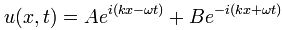
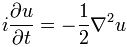
$\hat{E} \Psi = i\hbar\dfrac{\partial}{\partial t}\Psi = E\Psi$ Now if we plug that in the equation above, we get our time-dependent Schrödinger equation:

$i \hbar \frac{\partial}{\partial t}\Psi = \hat H \Psi$

OK. You probably did not understand one iota of this but, even then, you will object that this does not resemble the equation I wrote at the very beginning: i(∂u/∂t) = (-1/2)∇²u.

You’re right, but we only need one more step for that. If we leave out potential energy (so we assume a particle moving in free space), then the Hamiltonian can be written as:

$\hat{H} = -\frac{\hbar^2}{2m}\nabla^2$

You’ll ask me how this is done but I will be short on that: the relationship between energy and momentum is being used here (and so that’s where the 2m factor in the denominator comes from). However, I won’t say more about it because this post would become way too lengthy if I would include each and every derivation and, remember, I just want to get to the result because the derivations here are not the point: I want you to understand the functional form of the wave equation only. So, using the above identity and, OK, let’s be somewhat more complete and include potential energy once again, we can write the time-dependent wave equation as:

$i\hbar\frac{\partial}{\partial t}\Psi(\mathbf{r},t) = -\frac{\hbar^2}{2m}\nabla^2\Psi(\mathbf{r},t) + V(\mathbf{r},t)\Psi(\mathbf{r},t)$

Now, how is the equation above related to i(∂u/∂t) = (-1/2)∇²u? It’s a very simplified version of it: potential energy is, once again, assumed to be not relevant (so we’re talking a free particle again, with no external forces acting on it) but the real simplification is that we give m and ħ the value 1, so m = ħ = 1. Why?

Well… My initial idea was to do something similar as I did above and, hence, actually use a specific example with an actual functional form, just like we did for that the real-valued u(x, t) function. However, when I look at how long this post has become already, I realize I should not do that. In fact, I would just copy an example from somewhere else – probably Wikipedia once again, if only because their examples are usually nicely illustrated with graphs (and often animated graphs). So let me just refer you here to the other example given in the Wikipedia article on wave packets: that example uses that simplified i(∂u/∂t) = (-1/2)∇²u equation indeed. It actually uses the same initial condition:

However, because the wave equation is different, the wave packet behaves differently. It’s a so-called dispersive wave packet: it delocalizes. Its width increases over time and so, after a while, it just vanishes because it diffuses all over space. So there’s a solution to the wave equation, given this initial condition, but it’s just not stable – as a description of some particle that is (from a mathematical point of view – or even a physical point of view – there is no issue).

In any case, this probably all sounds like Chinese – or Greek if you understand Chinese :-). I actually haven’t worked with these Hermitian operators yet, and so it’s pretty shaky territory for me myself. However, I felt like I had picked up enough math and physics on this long and winding Road to Reality (I don’t think I am even halfway) to give it a try. I hope I succeeded in passing the message, which I’ll summarize as follows:

Schrödinger’s equation is just like any other differential equation used in physics, in the sense that it represents a system subject to constraints, such as the relationship between energy and momentum.
It will have many general solutions. In other words, the wave function – which describes a probability amplitude as a function in space and time – will have many general solutions, and a specific solution will depend on the initial conditions.
The solution(s) can represent stationary states, but not necessary so: a wave (or a wave packet) can be non-dispersive or dispersive. However, when we plug the wave function into the wave equation, it will satisfy that equation.

That’s neither spectacular nor difficult, is it? But, perhaps, it helps you to ‘understand’ wave equations, including the Schrödinger equation. But what is understanding? Dirac once famously said: “I consider that I understand an equation when I can predict the properties of its solutions, without actually solving it.”

Hmm… I am not quite there yet, but I am sure some more practice with it will help. 🙂

Post scriptum: On Maxwell’s equations

First, we should say something more about these two other operators which I introduced above: the divergence and the curl. First on the divergence.

The divergence of a field vector E (or B) at some point r represents the so-called flux of E, i.e. the ‘flow’ of E per unit volume. So flux and divergence both deal with the ‘flow’ of electric field lines away from (positive) charges. [The ‘away from’ is from positive charges indeed – as per the convention: Maxwell himself used the term ‘convergence’ to describe flow towards negative charges, but so his ‘convention’ did not survive. Too bad, because I think convergence would be much easier to remember.]

So if we write that ∇•E = ρ/ε₀, then it means that we have some constant flux of E because of some (fixed) distribution of charges.

Now, we already mentioned that equation (2) in Maxwell’s set meant that there is no such thing as a ‘magnetic’ charge: indeed, ∇•B = 0 means there is no magnetic flux. But, of course, magnetic fields do exist, don’t they? They do. A current in a wire, for example, i.e. a bunch of steadily moving electric charges, will induce a magnetic field according to Ampère’s law, which is part of equation (4) in Maxwell’s set: c²∇×B = j/ε₀, with j representing the current density and ε₀ the electric constant.

Now, at this point, we have this curl: ∇×B. Just like divergence (or convergence as Maxwell called it – but then with the sign reversed), curl also means something in physics: it’s the amount of ‘rotation’, or ‘circulation’ as Feynman calls it, around some loop.

So, to summarize the above, we have (1) flux (divergence) and (2) circulation (curl) and, of course, the two must be related. And, while we do not have any magnetic charges and, hence, no flux for B, the current in that wire will cause some circulation of B, and so we do have a magnetic field. However, that magnetic field will be static, i.e. it will not change. Hence, the time derivative ∂B/∂t will be zero and, hence, from equation (2) we get that ∇×E = 0, so our electric field will be static too. The time derivative ∂E/∂t which appears in equation (4) also disappears and we just have c²∇×B = j/ε₀. This situation – of a constant magnetic and electric field – is described as electrostatics and magnetostatics respectively. It implies a neat separation of the four equations, and it makes magnetism and electricity appear as distinct phenomena. Indeed, as long as charges and currents are static, we have:

[I] Electrostatics: (1) ∇•E = ρ/ε₀and (2) ∇×E = 0

[II] Magnetostatics: (3) c²∇×B = j/ε₀and (4) ∇•B = 0

The first two equations describe a vector field with zero curl and a given divergence (i.e. the electric field) while the third and fourth equations second describe a seemingly separate vector field with a given curl but zero divergence. Now, I am not writing this post scriptum to reproduce Feynman’s Lectures on Electromagnetism, and so I won’t say much more about this. I just want to note two points:

1. The first point to note is that factor c²in the c²∇×B = j/ε₀equation. That’s something which you don’t have in the ∇•E = ρ/ε₀equation. Of course, you’ll say: So what? Well… It’s weird. And if you bring it to the other side of the equation, it becomes clear that you need an awful lot of current for a tiny little bit of magnetic circulation (because you’re dividing by c² , so that’s a factor 9 with 16 zeroes after it (9×10¹⁶): an awfully big number in other words). Truth be said, it reveals something very deep. Hmm? Take a wild guess. […] Relativity perhaps? Well… Yes!

It’s obvious that we buried v somewhere in this equation, the velocity of the moving charges. But then it’s part of j of course: the rate at which charge flows through a unit area per second. But – Hey! – velocity as compared to what? What’s the frame of reference? The frame of reference is us obviously or – somewhat less subjective – the stationary charges determining the electric field according to equation (1) in the set above: ∇•E = ρ/ε₀. But so here we can ask the same question: stationary in what reference frame? As compared to the moving charges? Hmm… But so how does it work with relativity? I won’t copy Feynman’s 13th Lecture here, but so, in that lecture, he analyzes what happens to the electric and magnetic force when we look at the scene from another coordinate system – let’s say one that moves parallel to the wire at the same speed as the moving electrons, so – because of our new reference frame – the ‘moving electrons’ now appear to have no speed at all but, of course, our stationary charges will now seem to move.

What Feynman finds – and his calculations are very easy and straightforward – is that, while we will obviously insert different input values into Maxwell’s set of equations and, hence, get different values for the E and B fields, the actual physical effect – i.e. the final Lorentz force on a (charged) particle – will be the same. To be very specific, in a coordinate system at rest with respect to the wire (so we see charges move in the wire), we find a ‘magnetic’ force indeed, but in a coordinate system moving at the same speed of those charges, we will find an ‘electric’ force only. And from yet another reference frame, we will find a mixture of E and B fields. However, the physical result is the same: there is only one combined force in the end – the Lorentz force F = q(E + v×B) – and it’s always the same, regardless of the reference frame (inertial or moving at whatever speed – relativistic (i.e. close to c) or not).

In other words, Maxwell’s description of electromagnetism is invariant or, to say exactly the same in yet other words, electricity and magnetism taken together are consistent with relativity: they are part of one physical phenomenon: the electromagnetic interaction between (charged) particles. So electric and magnetic fields appear in different ‘mixtures’ if we change our frame of reference, and so that’s why magnetism is often described as a ‘relativistic’ effect – although that’s not very accurate. However, it does explain that c²factor in the equation for the curl of B. [How exactly? Well… If you’re smart enough to ask that kind of question, you will be smart enough to find the derivation on the Web. :-)]

Note: Don’t think we’re talking astronomical speeds here when comparing the two reference frames. It would also work for astronomical speeds but, in this case, we are talking the speed of the electrons moving through a wire. Now, the so-called drift velocity of electrons – which is the one we have to use here – in a copper wire of radius 1 mm carrying a steady current of 3 Amps is only about 1 m per hour! So the relativistic effect is tiny – but still measurable !

2. The second thing I want to note is that Maxwell’s set of equations with non-zero time derivatives for E and B clearly show that it’s changing electric and magnetic fields that sort of create each other, and it’s this that’s behind electromagnetic waves moving through space without losing energy. They just travel on and on. The math behind this is beautiful (and the animations in the related Wikipedia articles are equally beautiful – and probably easier to understand than the equations), but that’s stuff for another post. As the electric field changes, it induces a magnetic field, which then induces a new electric field, etc., allowing the wave to propagate itself through space. I should also note here that the energy is in the field and so, when electromagnetic waves, such as light, or radiowaves, travel through space, they carry their energy with them.

Let me be fully complete here, and note that there’s energy in electrostatic fields as well, and the formula for it is remarkably beautiful. The total (electrostatic) energy U in an electrostatic field generated by charges located within some finite distance is equal to:

This equation introduces the electrostatic potential. This is a scalar field Φ from which we can derive the electric field vector just by applying the gradient operator. In fact, all curl-free fields (such as the electric field in this case) can be written as the gradient of some scalar field. That’s a universal truth. See how beautiful math is? 🙂

End of the Road to Reality?

Pre-scriptum (dated 26 June 2020): This post did not suffer from the DMCA take-down of some material. It is, therefore, still quite readable—even if my views on these matters have evolved quite a bit as part of my realist interpretation of QM. I now think the idea of force-carrying particles (bosons) is quite medieval. Moreover, I think the Higgs particle and other bosons (except for the photon and the neutrino) are just short-lived transients or resonances. Disequilibrium states, in other words. One should not refer to them as particles.

Original post:

Or the end of theoretical physics?

In my previous post, I mentioned the Goliath of science and engineering: the Large Hadron Collider (LHC), built by the European Organization for Nuclear Research (CERN) under the Franco-Swiss border near Geneva. I actually started uploading some pictures, but then I realized I should write a separate post about it. So here we go.

The first image (see below) shows the LHC tunnel, while the other shows (a part of) one of the two large general-purpose particle detectors that are part of this Large Hadron Collider. A detector is the thing that’s used to look at those collisions. This is actually the smallest of the two general-purpose detectors: it’s the so-called CMS detector (the other one is the ATLAS detector), and it’s ‘only’ 21.6 meter long and 15 meter in diameter – and it weighs about 12,500 tons. But so it did detect a Higgs particle – just like the ATLAS detector. [That’s actually not 100% sure but it was sure enough for the Nobel Prize committee – so I guess that should be good enough for us common mortals :-)]

The picture above shows one of these collisions in the CMS detector. It’s not the one with the trace of the Higgs particle though. In fact, I have not found any image that actually shows the Higgs particle: the closest thing to such image are some impressionistic images on the ATLAS site. See http://atlas.ch/news/2013/higgs-into-fermions.html

In case you wonder what’s being scattered here… Well… All kinds of things – but so the original collision is usually between protons (so these are hydrogen ions: H⁺nuclei), although the LHC can produce other nucleon beams as well (collectively referred to as hadrons). These protons have energy levels of 4 TeV (tera-electronVolt: 1 TeV = 1000 GeV = 1 trillion eV = 1×10¹² eV).

Now, let’s think about scale once again. Remember (from that same previous post) that we calculated a wavelength of 0.33 nanometer (1 nm = 1×10^–9 m, so that’s a billionth of a meter) for an electron. Well, this LHC is actually exploring the sub-femtometer (fm) frontier. One femtometer (fm) is 1×10^–15 m so that’s another million times smaller. Yes: so we are talking a millionth of a billionth of a meter. The size of a proton is an estimated 1.7 femtometer indeed and, as you surely know, a proton is a point-like thing occupying a very tiny space, so it’s not like an electron ‘cloud’ swirling around: it’s much smaller. In fact, quarks – three of them make up a proton (or a neutron) – are usually thought of as being just a little bit less than half that size – so that’s about 0.7 fm.

It may also help you to use the value I mentioned for high-energy electrons when I was discussing the LEP (the Large Electron-Positron Collider, which preceded the LHC) – so that was 104.5 GeV – and calculate the associated de Broglie wavelength using E = hf and λ = v/f. The velocity v is close to c and, hence, if we plug everything in, we get a value close to 1.2×10^–15 m indeed, so that’s the femtometer scale indeed. [If you don’t want to calculate anything, then just note we’re going from eV to giga-eV energy levels here, and so our wavelength decreases accordingly: one billion times smaller. Also remember (from the previous posts) that we calculated a wavelength of 0.33×10^–6 m and an associated energy level of 70 eV for a slow-moving electron – i.e. one going at 2200 km per second ‘only’, i.e. less than 1% of the speed of light.] Also note that, at these energy levels, it doesn’t matter whether or not we include the rest mass of the electron: 0.511 MeV is nothing as compared to the GeV realm. In short, we are talking very very tiny stuff here.

But so that’s the LEP scale. I wrote that the LHC is probing things at the sub-femtometer scale. So how much sub-something is that? Well… Quite a lot: the LHC is looking at stuff at a scale that’s more than a thousand times smaller. Indeed, if collision experiments in the giga-electronvolt (GeV) energy range correspond to probing stuff at the femtometer scale, then tera-electronvolt (TeV) energy levels correspond to probing stuff that’s, once again, another thousand times smaller, so we’re looking at distances of less than a thousandth of a millionth of a billionth of a meter. Now, you can try to ‘imagine’ that, but you can’t really.

So what do we actually ‘see’ then? Well… Nothing much one could say: all we can ‘see’ are traces of point-like ‘things’ being scattered, which then disintegrate or just vanish from the scene – as shown in the image above. In fact, as mentioned above, we do not even have such clear-cut ‘trace’ of a Higgs particle: we’ve got a ‘kinda signal’ only. So that’s it? Yes. But then these images are beautiful, aren’t they? If only to remind ourselves that particle physics is about more than just a bunch of formulas. It’s about… Well… The essence of reality: its intrinsic nature so to say. So… Well…

Let me be skeptical. So we know all of that now, don’t we? The so-called Standard Model has been confirmed by experiment. We now know how Nature works, don’t we? We observe light (or, to be precise, radiation: most notably that cosmic background radiation that reaches us from everywhere) that originated nearly 14 billion years ago (to be precise: 380,000 years after the Big Bang – but what’s 380,000 years on this scale?) and so we can ‘see’ things that are 14 billion light-years away. In fact, things that were 14 billion light-years away: indeed, because of the expansion of the universe, they are further away now and so that’s why the so-called observable universe is actually larger. So we can ‘see’ everything we need to ‘see’ at the cosmic distance scale and now we can also ‘see’ all of the particles that make up matter, i.e. quarks and electrons mainly (we also have some other so-called leptons, like neutrinos and muons), and also all of the particles that make up anti-matter of course (i.e. antiquarks, positrons etcetera). As importantly – or even more – we can also ‘see’ all of the ‘particles’ carrying the forces governing the interactions between the ‘matter particles’ – which are collectively referred to as fermions, as opposed to the ‘force carrying’ particles, which are collectively referred to as bosons (see my previous post on Bose and Fermi). Let me quickly list them – just to make sure we’re on the same page:

Photons for the electromagnetic force.
Gluons for the so-called strong force, which explains why positively charged protons ‘stick’ together in nuclei – in spite of their electric charge, which should push them away from each other. [You might think it’s the neutrons that ‘glue’ them together but so, no, it’s the gluons.]
W⁺, W^–, and Z bosons for the so-called ‘weak’ interactions (aka as Fermi’s interaction), which explain how one type of quark can change into another, thereby explaining phenomena such as beta decay. [For example, carbon-14 will – through beta decay – spontaneously decay into nitrogen-14. Indeed, carbon-12 is the stable isotope, while carbon-14 has a life-time of 5,730 ± 40 years ‘only’ 🙂 and, hence, measuring how much carbon-14 is left in some organic substance allows us to date it (that’s what (radio)carbon-dating is about). As for the name, a beta particle can refer to an electron or a positron, so we can have β^– decay (e.g. the above-mentioned carbon-14 decay) as well as β⁺decay (e.g. magnesium-23 into sodium-23). There’s also alpha and gamma decay but that involves different things. In any case… Let me end this digression within the digression.]
Finally, the existence of the Higgs particle – and, hence, of the associated Higgs field – has been predicted since 1964 already, but so it was only experimentally confirmed (i.e. we saw it, in the LHC) last year, so Peter Higgs – and a few others of course – got their well-deserved Nobel prize only 50 years later. The Higgs field gives fermions, and also the W⁺, W^–, and Z bosons, mass (but not photons and gluons, and so that’s why the weak force has such short range – as compared to the electromagnetic and strong forces).

So there we are. We know it all. Sort of. Of course, there are many questions left – so it is said. For example, the Higgs particle does actually not explain the gravitational force, so it’s not the (theoretical) graviton, and so we do not have a quantum field theory for the gravitational force. [Just Google it and you’ll see why: there’s theoretical as well as practical (experimental) reasons for that.] Secondly, while we do have a quantum field theory for all of the forces (or ‘interactions’ as physicists prefer to call them), there are a lot of constants in them (much more than just that Planck constant I introduced in my posts!) that seem to be ‘unrelated and arbitrary.’ I am obviously just quoting Wikipedia here – but it’s true.

Just look at it: three ‘generations’ of matter with various strange properties, four force fields (and some ‘gauge theory’ to provide some uniformity), bosons that have mass (the W⁺, W^–, and Z bosons, and then the Higgs particle itself) but then photons and gluons don’t… It just doesn’t look good, and then Feynman himself wrote, just a few years before his death (QED, 1985, p. 128), that the math behind calculating some of these constants (the coupling constant j for instance, or the rest mass n of an electron), which he actually invented (it makes use of a mathematical approximation method called perturbation theory) and for which he got a Nobel Prize, is a “dippy process” and that “having to resort to such hocus-pocus has prevented us from proving that the theory of quantum electrodynamics is mathematically self-consistent“. He adds: “It’s surprising that the theory still hasn’t been proved self-consistent one way or the other by now; I suspect that renormalization [“the shell game that we play to find n and j” as he calls it] is not mathematically legitimate.” And so he writes this about quantum electrodynamics, not about “the rest of physics” (and so that’s quantum chromodynamics (QCD) – the theory of the strong interactions – and quantum flavordynamics (QFD) – the theory of weak interactions) which, he adds, “has not been checked anywhere near as well as electrodynamics.”

Waw ! That’s a pretty damning statement, isn’t it? In short, all of the celebrations around the experimental confirmation of the Higgs particle cannot hide the fact that it all looks a bit messy. There are other questions as well – most of which I don’t understand so I won’t mention them. To make a long story short, physicists and mathematicians alike seem to think there must be some ‘more fundamental’ theory behind. But – Hey! – you can’t have it all, can you? And, of course, all these theoretical physicists and mathematicians out there do need to justify their academic budget, don’t they? And so all that talk about a Grand Unification Theory (GUT) is probably just what is it: talk. Isn’t it? Maybe.

The key question is probably easy to formulate: what’s beyond this scale of a thousandth of a proton diameter (0.001×10^–15m) – a thousandth of a millionth of a billionth of a meter that is. Well… Let’s first note that this so-called ‘beyond’ is a ‘universe’ which mankind (or let’s just say ‘we’) will never see. Never ever. Why? Because there is no way to go substantially beyond the 4 TeV energy levels that were reached last year – at great cost – in the world’s largest particle collider (the LHC). Indeed, the LHC is widely regarded not only as “the most complex and ambitious scientiﬁc project ever accomplished by humanity” (I am quoting a CERN scientist here) but – with a cost of more than 7.5 billion Euro – also as one of the most expensive ones. Indeed, taking into account inflation and all that, it was like the Manhattan project indeed (although scientists loathe that comparison). So we should not have any illusions: there will be no new super-duper LHC any time soon, and surely not during our lifetime: the current LHC is the super-duper thing!

Indeed, when I write ‘substantially‘ above, I really mean substantially. Just to put things in perspective: the LHC is currently being upgraded to produce 7 TeV beams (it was shut down for this upgrade, and it should come back on stream in 2015). That sounds like an awful lot (from 4 to 7 is +75%), and it is: it amounts to packing the kinetic energy of seven flying mosquitos (instead of four previously :-)) into each and every particle that makes up the beam. But that’s not substantial, in the sense that it is very much below the so-called GUT energy scale, which is the energy level above which, it is believed (by all those GUT theorists at least), the electromagnetic force, the weak force and the strong force will all be part and parcel of one and the same unified force. Don’t ask me why (I’ll know when I finished reading Penrose, I hope) but that’s what it is (if I should believe what I am reading currently that is). In any case, the thing to remember is that the GUT energy levels are in the 10¹⁶ GeV range, so that’s – sorry for all these numbers – a trillion TeV. That amounts to pumping more than 160,000 Joule in each of those tiny point-like particles that make up our beam. So… No. Don’t even try to dream about it. It won’t happen. That’s science fiction – with the emphasis on fiction. [Also don’t dream about a trillion flying mosquitos packed into one proton-sized super-mosquito either. :-)]

So what?

Well… I don’t know. Physicists refer to the zone beyond the above-mentioned scale (so things smaller than 0.001×10^–15m) as the Great Desert. That’s a very appropriate name I think – for more than one reason. And so it’s this ‘desert’ that Roger Penrose is actually trying to explore in his ‘Road to Reality’. As for me, well… I must admit I have great trouble following Penrose on this road. I’ve actually started to doubt that Penrose’s Road leads to Reality. Maybe it takes us away from it. Huh? Well… I mean… Perhaps the road just stops at that 0.001×10^–15m frontier?

In fact, that’s a view which one of the early physicists specialized in high-energy physics, Raoul Gatto, referred to as the zeroth scenario. I am actually not quoting Gatto here, but another theoretical physicist: Gerard ‘t Hooft, another Nobel prize winner (you may know him better because he’s a rather fervent Mars One supporter, but so here I am referring to his popular 1996 book In Search of the Ultimate Building Blocks). In any case, Gatto, and most other physicists, including ‘T Hooft (despite the fact ‘T Hooft got his Nobel prize for his contribution to gauge theory – which, together with Feynman’s application of perturbation theory to QED, is actually the backbone of the Standard Model) firmly reject this zeroth scenario. ‘T Hooft himself thinks superstring theory (i.e. supersymmetric string theory – which has now been folded into M-theory or – back to the original term – just string theory – the terminology is quite confusing) holds the key to exploring this desert.

But who knows? In fact, we can’t – because of the above-mentioned practical problem of experimental confirmation. So I am likely to stay on this side of the frontier for quite a while – if only because there’s still so much to see here and, of course, also because I am just at the beginning of this road. 🙂 And then I also realize I’ll need to understand gauge theory and all that to continue on this road – which is likely to take me another six months or so (if not more) and then, only then, I might try to look at those little strings, even if we’ll never see them because… Well… Their theoretical diameter is the so-called Planck length. So what? Well… That’s equal to 1.6×10⁻³⁵m. So what? Well… Nothing. It’s just that 1.6×10⁻³⁵m is 1/10 000 000 000 000 000 of that sub-femtometer scale. I don’t even want to write this in trillionths of trillionths of trillionths etcetera because I feel that’s just not making any sense. And perhaps it doesn’t. One thing is for sure: that ‘desert’ that GUT theorists want us to cross is not just ‘Great’: it’s ENORMOUS!

Richard Feynman – another Nobel Prize scientist whom I obviously respect a lot – surely thought trying to cross a desert like that amounts to certain death. Indeed, he’s supposed to have said the following about string theorists, about a year or two before he died (way too young): “I don’t like that they’re not calculating anything. I don’t like that they don’t check their ideas. I don’t like that for anything that disagrees with an experiment, they cook up an explanation–a fix-up to say, “Well, it might be true.” For example, the theory requires ten dimensions. Well, maybe there’s a way of wrapping up six of the dimensions. Yes, that’s all possible mathematically, but why not seven? When they write their equation, the equation should decide how many of these things get wrapped up, not the desire to agree with experiment. In other words, there’s no reason whatsoever in superstring theory that it isn’t eight out of the ten dimensions that get wrapped up and that the result is only two dimensions, which would be completely in disagreement with experience. So the fact that it might disagree with experience is very tenuous, it doesn’t produce anything; it has to be excused most of the time. It doesn’t look right.”

Hmm… Feynman and ‘T Hooft… Two giants in science. Two Nobel Prize winners – and for stuff that truly revolutionized physics. The amazing thing is that those two giants – who are clearly at loggerheads on this one – actually worked closely together on a number of other topics – most notably on the so-called Feynman-‘T Hooft gauge, which – as far as I understand – is the one that is most widely used in quantum field calculations. But I’ll leave it at that here – and I’ll just make a mental note of the terminology here. The Great Desert… Probably an appropriate term. ‘T Hooft says that most physicists think that desert is full of tiny flowers. I am not so sure – but then I am not half as smart as ‘T Hooft. Much less actually. So I’ll just see where the road I am currently following leads me. With Feynman’s warning in mind, I should probably expect the road condition to deteriorate quickly.

Post scriptum: You will not be surprised to hear that there’s a word for 1×10^–18m: it’s called an attometer (with two t’s, and abbreviated as am). And beyond that we have zeptometer (1 zm = 1×10^–21m) and yoctometer (1 ym = 1×10^–23m). In fact, these measures actually represent something: 20 yoctometer is the estimated radius of a 1 MeV neutrino – or, to be precise, its the radius of the cross section, which is “the effective area that governs the probability of some scattering or absorption event.” But so then there are no words anymore. The next measure is the Planck length: 1.62 × 10⁻³⁵ m – but so that’s a trillion (10¹²) times smaller than a yoctometer. Unimaginable, isn’t it? Literally.

Note: A 1 MeV neutrino? Well… Yes. The estimated rest mass of an (electron) neutrino is tiny: at least 50,000 times smaller than the mass of the electron and, therefore, neutrinos are often assumed to be massless, for all practical purposes that is. However, just like the massless photon, they can carry high energy. High-energy gamma ray photons, for example, are also associated with MeV energy levels. Neutrinos are one of the many particles produced in high-energy particle collisions in particle accelerators, but they are present everywhere: they’re produced by stars (which, as you know, are nuclear fusion reactors). In fact, most neutrinos passing through Earth are produced by our Sun. The largest neutrino detector on Earth is called IceCube. It sits on the South Pole – or under it, as it’s suspended under the Antarctic ice, and it regularly captures high-energy neutrinos in the range of 1 to 10 TeV. Last year (in November 2013), it captured two with energy levels around 1000 TeV – so that’s the peta-electronvolt level (1 PeV = 1×10¹⁵eV). If you think that’s amazing, it is. But also remember that 1 eV is 1.6×10⁻¹⁹Joule, so it’s ‘only’ a ten-thousandth of a Joule. In other words, you would need at least ten thousand of them to briefly light up an LED. The PeV pair was dubbed Bert and Ernie and the illustration below (from IceCube’s website) conveys how the detectors sort of lit up when they passed. It was obviously a pretty clear ‘signal’ – but so the illustration also makes it clear that we don’t really ‘see’ at such small scale: we just know ‘something’ happened.

The Uncertainty Principle re-visited: Fourier transforms and conjugate variables

Pre-scriptum (dated 26 June 2020): This post did not suffer from the DMCA take-down of some material. It is, therefore, still quite readable—even if my views on the nature of the Uncertainty Principle have evolved quite a bit as part of my realist interpretation of QM.

Original post:

In previous posts, I presented a time-independent wave function for a particle (or wavicle as we should call it – but so that’s not the convention in physics) – let’s say an electron – traveling through space without any external forces (or force fields) acting upon it. So it’s just going in some random direction with some random velocity v and, hence, its momentum is p = mv. Let me be specific – so I’ll work with some numbers here – because I want to introduce some issues related to units for measurement.

So the momentum of this electron is the product of its mass m (about 9.1×10⁻²⁸ grams) with its velocity v (typically something in the range around 2,200 km/s, which is fast but not even close to the speed of light – and, hence, we don’t need to worry about relativistic effects on its mass here). Hence, the momentum p of this electron would be some 20×10⁻²⁵ kg·m/s. Huh? Kg·m/s?Well… Yes, kg·m/s or N·s are the usual measures of momentum in classical mechanics: its dimension is [mass][length]/[time] indeed. However, you know that, in atomic physics, we don’t want to work with these enormous units (because we then always have to add these ×10⁻²⁸ and ×10⁻²⁵ factors and so that’s a bit of a nuisance indeed). So the momentum p will usually be measured in eV/c, with c representing what it usually represents, i.e. the speed of light. Huh? What’s this strange unit? Electronvolts divided by c? Well… We know that eV is an appropriate unit for measuring energy in atomic physics: we can express eV in Joule and vice versa: 1 eV = 1.6×10⁻¹⁹Joule, so that’s OK – except for the fact that this Joule is a monstrously large unit at the atomic scale indeed, and so that’s why we prefer electronvolt. But the Joule is a shorthand unit for kg·m²/s², which is the measure for energy expressed in SI units, so there we are: while the SI dimension for energy is actually [mass][length]²/[time]², using electronvolts (eV) is fine. Now, just divide the SI dimension for energy, i.e. [mass][length]²/[time]², by the SI dimension for velocity, i.e. [length]/[time]: we get something expressed in [mass][length]/[time]. So that’s the SI dimension for momentum indeed! In other words, dividing some quantity expressed in some measure for energy (be it Joules or electronvolts or erg or calories or coulomb-volts or BTUs or whatever – there’s quite a lot of ways to measure energy indeed!) by the speed of light (c) will result in some quantity with the right dimensions indeed. So don’t worry about it. Now, 1 eV/c is equivalent to 5.344×10⁻²⁸ kg·m/s, so the momentum of this electron will be 3.75 eV/c.

Let’s go back to the main story now. Just note that the momentum of this electron that we are looking at is a very tiny amount – as we would expect of course.

Time-independent means that we keep the time variable (t) in the wave function Ψ(x, t) fixed and so we only look at how Ψ(x, t) varies in space, with x as the (real) space variable representing position. So we have a simplified wave function Ψ(x) here: we can always put the time variable back in when we’re finished with the analysis. By now, it should also be clear that we should distinguish between real-valued wave functions and complex-valued wave functions. Real-valued wave functions represent what Feynman calls “real waves”, like a sound wave, or an oscillating electromagnetic field. Complex-valued wave functions describe probability amplitudes. They are… Well… Feynman actually stops short of saying that they are not real. So what are they?

They are, first and foremost complex numbers, so they have a real and a so-called imaginary part (z = a + ib or, if we use polar coordinates, re^θ= cosθ + isinθ). Now, you may think – and you’re probably right to some extent – that the distinction between ‘real’ waves and ‘complex’ waves is, perhaps, less of a dichotomy than popular writers – like me 🙂 – suggest. When describing electromagnetic waves, for example, we need to keep track of both the electric field vector E as well as the magnetic field vector B (both are obviously related through Maxwell’s equations). So we have two components as well, so to say, and each of these components has three dimensions in space, and we’ll use the same mathematical tools to describe them (so we will also represent them using complex numbers). That being said, these probability amplitudes, usually denoted by Ψ(x), describe something very different. What exactly? Well… By now, it should be clear that that is actually hard to explain: the best thing we can do is to work with them, so they start feeling familiar. The main thing to remember is that we need to square their modulus (or magnitude or absolute value if you find these terms more comprehensible) to get a probability (P). For example, the expression below gives the probability of finding a particle – our electron for example – in in the (space) interval [a, b]:

Of course, we should not be talking intervals but three-dimensional regions in space. However, we’ll keep it simple: just remember that the analysis should be extended to three (space) dimensions (and, of course, include the time dimension as well) when we’re finished (to do that, we’d use so-called four-vectors – another wonderful mathematical invention).

Now, we also used a simple functional form for this wave function, as an example: Ψ(x) could be proportional, we said, to some idealized function e^ikx. So we can write: Ψ(x) ∝ e^ikx (∝ is the standard symbol expressing proportionality). In this function, we have a wave number k, which is like the frequency in space of the wave (but then measured in radians because the phase of the wave function has to be expressed in radians). In fact, we actually wrote Ψ(x, t) = (1/x)e^{i(kx – ωt)}(so the magnitude of this amplitude decreases with distance) but, again, let’s keep it simple for the moment: even with this very simple function e^ikx , things will become complex enough.

We also introduced the de Broglie relation, which gives this wave number k as a function of the momentum p of the particle: k = p/ħ, with ħ the (reduced) Planck constant, i.e. a very tiny number in the neighborhood of 6.582 ×10⁻¹⁶ eV·s. So, using the numbers above, we’d have a value for k equal to 3.75 eV/c divided by 6.582 ×10⁻¹⁶ eV·s. So that’s 0.57×10¹⁶ (radians) per… Hey, how do we do it with the units here? We get an incredibly huge number here (57 with 14 zeroes after it) per second? We should get some number per meter because k is expressed in radians per unit distance, right? Right. We forgot c. We are actually measuring distance here, but in light-seconds instead of meter: k is 0.57×10¹⁶/c·s. Indeed, a light-second is the distance traveled by light in one second, so that’s c·s, and if we want k expressed in radians per meter, then we need to divide this huge number 0.57×10¹⁶ (in rad) by 2.998×10⁸( in (m/s)·s) and so then we get a much more reasonable value for k, and with the right dimension too: to be precise, k is about 19×10⁶ rad/m in this case. That’s still huge: it corresponds with a wavelength of 0.33 nanometer (1 nm = 10^-6 m) but that’s the correct order of magnitude indeed.

[In case you wonder what formula I am using to calculate the wavelength: it’s λ = 2π/k. Note that our electron’s wavelength is more than a thousand times shorter than the wavelength of (visible) light (we humans can see light with wavelengths ranging from 380 to 750 nm) but so that’s what gives the electron its particle-like character! If we would increase their velocity (e.g. by accelerating them in an accelerator, using electromagnetic fields to propel them to speeds closer to c and also to contain them in a beam), then we get hard beta rays. Hard beta rays are surely not as harmful as high-energy electromagnetic rays. X-rays and gamma rays consist of photons with wavelengths ranging from 1 to 100 picometer (1 pm = 10^–12m) – so that’s another factor of a thousand down – and thick lead shields are needed to stop them: they are the cause of cancer (Marie Curie’s cause of death), and the hard radiation of a nuclear blast will always end up killing more people than the immediate blast effect. In contrast, hard beta rays will cause skin damage (radiation burns) but they won’t go deeper than that.]

Let’s get back to our wave function Ψ(x) ∝ e^ikx. When we introduced it in our previous posts, we said it could not accurately describe a particle because this wave function (Ψ(x) = Ae^ikx) is associated with probabilities |Ψ(x)|² that are the same everywhere. Indeed, |Ψ(x)|² = |Ae^ikx|² = A². Apart from the fact that these probabilities would add up to infinity (so this mathematical shape is unacceptable anyway), it also implies that we cannot locate our electron somewhere in space. It’s everywhere and that’s the same as saying it’s actually nowhere. So, while we can use this wave function to explain and illustrate a lot of stuff (first and foremost the de Broglie relations), we actually need something different if we would want to describe anything real (which, in the end, is what physicists want to do, right?). We already said in our previous posts: real particles will actually be represented by a wave packet, or a wave train. A wave train can be analyzed as a composite wave consisting of a (potentially infinite) number of component waves. So we write:

Note that we do not have one unique wave number k or – what amounts to saying the same – one unique value p for the momentum: we have n values. So we’re introducing a spread in the wavelength here, as illustrated below:

In fact, the illustration above talks of a continuous distribution of wavelengths and so let’s take the continuum limit of the function above indeed and write what we should be writing:

Now that is an interesting formula. [Note that I didn’t care about normalization issues here, so it’s not quite what you’d see in a more rigorous treatment of the matter. I’ll correct that in the Post Scriptum.] Indeed, it shows how we can get the wave function Ψ(x) from some other function Φ(p). We actually encountered that function already, and we referred to it as the wave function in the momentum space. Indeed, Nature does not care much what we measure: whether it’s position (x) or momentum (p), Nature will not share her secrets with us and, hence, the best we can do – according to quantum mechanics – is to find some wave function associating some (complex) probability amplitude with each and every possible (real) value of x or p. What the equation above shows, then, is these wave functions come as a pair: if we have Φ(p), then we can calculate Ψ(x) – and vice versa. Indeed, the particular relation between Ψ(x) and Φ(p) as established above, makes Ψ(x) and Φ(p) a so-called Fourier transform pair, as we can transform Φ(p) into Ψ(x) using the above Fourier transform (that’s how that integral is called), and vice versa. More in general, a Fourier transform pair can be written as:

Instead of x and p, and Ψ(x) and Φ(p), we have x and y, and f(x) and g(y), in the formulas above, but so that does not make much of a difference when it comes to the interpretation: x and p (or x and y in the formulas above) are said to be conjugate variables. What it means really is that they are not independent. There are quite a few of such conjugate variables in quantum mechanics such as, for example: (1) time and energy (and time and frequency, of course, in light of the de Broglie relation between both), and (2) angular momentum and angular position (or orientation). There are other pairs too but these involve quantum-mechanical variables which I do not understand as yet and, hence, I won’t mention them here. [To be complete, I should also say something about that 1/2π factor, but so that’s just something that pops up when deriving the Fourier transform from the (discrete) Fourier series on which it is based. We can put it in front of either integral, or split that factor across both. Also note the minus sign in the exponent of the inverse transform.]

When you look at the equations above, you may think that f(x) and g(y) must be real-valued functions. Well… No. The Fourier transform can be used for both real-valued as well as complex-valued functions. However, at this point I’ll have to refer those who want to know each and every detail about these Fourier transforms to a course in complex analysis (such as Brown and Churchill’s Complex Variables and Applications (2004) for instance) or, else, to a proper course on real and complex Fourier transforms (they are used in signal processing – a very popular topic in engineering – and so there’s quite a few of those courses around).

The point to note in this post is that we can derive the Uncertainty Principle from the equations above. Indeed, the (complex-valued) functions Ψ(x) and Φ(p) describe (probability) amplitudes, but the (real-valued) functions |Ψ(x)|² and |Φ(p)|² describe probabilities or – to be fully correct – they are probability (density) functions. So it is pretty obvious that, if the functions Ψ(x) and Φ(p) are a Fourier transform pair, then |Ψ(x)|² and |Φ(p)|² must be related to. They are. The derivation is a bit lengthy (and, hence, I will not copy it from the Wikipedia article on the Uncertainty Principle) but one can indeed derive the so-called Kennard formulation of the Uncertainty Principle from the above Fourier transforms. This Kennard formulation does not use this rather vague Δx and Δp symbols but clearly states that the product of the standard deviation from the mean of these two probability density functions can never be smaller than ħ/2:

σ_xσ_p≥ ħ/2

To be sure: ħ/2 is a rather tiny value, as you should know by now, 🙂 but, so, well… There it is.

As said, it’s a bit lengthy but not that difficult to do that derivation. However, just for once, I think I should try to keep my post somewhat shorter than usual so, to conclude, I’ll just insert one more illustration here (yes, you’ve seen that one before), which should now be very easy to understand: if the wave function Ψ(x) is such that there’s relatively little uncertainty about the position x of our electron, then the uncertainty about its momentum will be huge (see the top graphs). Vice versa (see the bottom graphs), precise information (or a narrow range) on its momentum, implies that its position cannot be known.

Does all this math make it any easier to understand what’s going on? Well… Yes and no, I guess. But then, if even Feynman admits that he himself “does not understand it the way he would like to” (Feynman Lectures, Vol. III, 1-1), who am I? In fact, I should probably not even try to explain it, should I? 🙂

So the best we can do is try to familiarize ourselves with the language used, and so that’s math for all practical purposes. And, then, when everything is said and done, we should probably just contemplate Mario Livio’s question: Is God a mathematician? 🙂

Post scriptum:

I obviously cut corners above, and so you may wonder how that ħ factor can be related to σ_xand σ _pif it doesn’t appear in the wave functions. Truth be told, it does. Because of (i) the presence of ħ in the exponent in our e^i(p/ħ)x function, (ii) normalization issues (remember that probabilities (i.e. Ψ|(x)|² and |Φ(p)|²) have to add up to 1) and, last but not least, (iii) the 1/2π factor involved in Fourier transforms , Ψ(x) and Φ(p) have to be written as follows:

Note that we’ve also re-inserted the time variable here, so it’s pretty complete now. One more thing we could do is to substitute x for a proper three-dimensional space vector x or, better still, introduce four-vectors, which would allow us to also integrate relativistic effects (most notably the slowing of time with motion – as observed from the stationary reference frame) – which become important when, for instance, we’re looking at electrons being accelerated, which is the rule, rather than the exception, in experiments.

Remember (from a previous post) that we calculated that an electron traveling at its usual speed in orbit (2200 km/s, i.e. less than 1% of the speed of light) had an energy of about 70 eV? Well, the Large Electron-Positron Collider (LEP) did accelerate them to speeds close to light, thereby giving them energy levels topping 104.5 billion eV (or 104.5 GeV as it’s written) so they could hit each other with collision energies topping 209 GeV (they come from opposite directions so it’s two times 104.5 GeV). Now, 209 GeV is tiny when converted to everyday energy units: 209 GeV is 33×10^–9Joule only indeed – and so note the minus sign in the exponent here: we’re talking billionths of a Joule here. Just to put things into perspective: 1 Watt is the energy consumption of an LED (and 1 Watt is 1 Joule per second), so you’d need to combine the energy of billions of these fast-traveling electrons to power just one little LED lamp. But, of course, that’s not the right comparison: 104.5 GeV is more than 200,000 times the electron’s rest mass (0.511 MeV), so that means that – in practical terms – their mass (remember that mass is a measure for inertia) increased by the same factor (204,500 times to be precise). Just to give an idea of the effort that was needed to do this: CERN’s LEP collider was housed in a tunnel with a circumference of 27 km. Was? Yes. The tunnel is still there but it now houses the Large Hadron Collider (LHC) which, as you surely know, is the world’s largest and most powerful particle accelerator: its experiments confirmed the existence of the Higgs particle in 2013, thereby confirming the so-called Standard Model of particle physics. [But I’ll see a few things about that in my next post.]

Oh… And, finally, in case you’d wonder where we get the inequality sign in σ_xσ_p≥ ħ/2, that’s because – at some point in the derivation – one has to use the Cauchy-Schwarz inequality (aka as the triangle inequality): |z₁+ z₁| ≤ |z₁|+| z₁|. In fact, to be fully complete, the derivation uses the more general formulation of the Cauchy-Schwarz inequality, which also applies to functions as we interpret them as vectors in a function space. But I would end up copying the whole derivation here if I add any more to this – and I said I wouldn’t do that. 🙂 […]

Bose and Fermi

Pre-scriptum (dated 26 June 2020): This post suffered from the DMCA take-down of material from Feynman’s Lectures, so some graphs are lacking and the layout was altered as a result. In any case, I now think the distinction between bosons and fermions is one of the most harmful scientific myths in physics. I deconstructed quite a few myths in my realist interpretation of QM, but I focus on this myth in particular in this paper: Feynman’s Worst Jokes and the Boson-Fermion Theory.

Original post:

Probability amplitudes: what are they?

Instead of reading Penrose, I’ve started to read Richard Feynman again. Of course, reading the original is always better than whatever others try to make of that, so I’d recommend you read Feynman yourself – instead of this blog. But then you’re doing that already, aren’t you? 🙂

Let’s explore those probability amplitudes somewhat more. They are complex numbers. In a fine little book on quantum mechanics (QED, 1985), Feynman calls them ‘arrows’ – and that’s what they are: two-dimensional vectors, aka complex numbers. So they have a direction and a length (or magnitude). When talking amplitudes, the direction and length are known as the phase and the modulus (or absolute value) respectively and you also know by now that the modulus squared represents a probability or probability density, such as the probability of detecting some particle (a photon or an electron) at some location x or some region Δx, or the probability of some particle going from A to B, or the probability of a photon being emitted or absorbed by an electron (or a proton), etcetera. I’ve inserted two illustrations below to explain the matter.

The first illustration just shows what a complex number really is: a two-dimensional number (z) with a real part (Re(z) = x) and an imaginary part (Im(z) = y). We can represent it in two ways: one uses the (x, y) coordinate system (z = x + iy), and the other is the so-called polar form: z = reⁱ^φ. The (real) number e in the latter equation is just Euler’s number, so that’s a mathematical constant (just like π). The little i is the imaginary unit, so that’s the thing we introduce to add a second (vertical) dimension to our analysis: i can be written as 0+i = (0, 1) indeed, and so it’s like a (second) basis vector in the two-dimensional (Cartesian or complex) plane.

I should not say much more about this, but I must list some essential properties and relationships:

The coordinate and polar form are related through Euler’s formula: z = x + iy = reⁱ^φ= r(cosφ + isinφ).
From this, and the fact that cos(-φ) = cosφ and sin(-φ) = –sinφ, it follows that the (complex) conjugate z* = x – iy of a complex number z = x + iy is equal to z* = re^–iφ. [I use z* as a symbol, instead of z-bar, because I can’t find a z-bar in the character set here.] This equality is illustrated above.
The length/modulus/absolute value of a complex number is written as |z| and is equal to |z| = (x² + y²)^1/2 = |reⁱ^φ| = r (so r is always a positive (real) number).
As you can see from the graph, a complex number z and its conjugate z* have the same absolute value: |z| = |x+iy| = |z*| = |x-iy|.
Therefore, we have the following: |z||z|=|z*||z*|=|z||z*|=|z|², and we can use this result to calculate the (multiplicative) inverse: z^-1 = 1/z = z*/|z|².
The absolute value of a product of complex numbers equals the product of the absolute values of those numbers: |z₁z₂| = |z₁||z₂|.
Last but not least, it is important to be aware of the geometric interpretation of the sum and the product of two complex numbers:
- The sum of two complex numbers amounts to adding vectors, so that’s the familiar parallelogram law for vector addition: (a+ib) + (c+id) = (a+b) + i(c+d).
- Multiplying two complex numbers amounts to adding the angles and multiplying their lengths – as evident from writing such product in its polar form: reⁱ^θseⁱ^Θ= rseⁱ⁽^θ+^Θ). The result is, quite obviously, another complex number. So it is not the usual scalar or vector product which you may or may not be familiar with.

[For the sake of completeness: (i) the scalar product (aka dot product) of two vectors (a•b) is equal to the product of is the product of the magnitudes of the two vectors and the cosine of the angle between them: a•b = |a||b|cosα; and (ii) the result of a vector product (or cross product) is a vector which is perpendicular to both, so it’s a vector that is not in the same plane as the vectors we are multiplying: a×b = |a||b| sinα n, with n the unit vector perpendicular to the plane containing a and b in the direction given by the so-called right-hand rule. Just be aware of the difference.]

The second illustration (see below) comes from that little book I mentioned above already: Feynman’s exquisite 1985 Alix G. Mautner Memorial Lectures on Quantum Electrodynamics, better known as QED: the Strange Theory of Light and Matter. It shows how these probability amplitudes, or ‘arrows’ as he calls them, really work, without even mentioning that they are ‘probability amplitudes’ or ‘complex numbers’. That being said, these ‘arrows’ are what they are: probability amplitudes.

To be precise, the illustration below shows the probability amplitude of a photon (so that’s a little packet of light) reflecting from the front surface (front reflection arrow) and the back (back reflection arrow) of a thin sheet of glass. If we write these vectors in polar form (reⁱ^φ), then it is obvious that they have the same length (r = 0.2) but their phase φ is different. That’s because the photon needs to travel a bit longer to reach the back of the glass: so the phase varies as a function of time and space, but the length doesn’t. Feynman visualizes that with the stopwatch: as the photon is emitted from a light source and travels through time and space, the stopwatch turns and, hence, the arrow will point in a different direction.

[To be even more precise, the amplitude for a photon traveling from point A to B is a (fairly simple) function (which I won’t write down here though) which depends on the so-called spacetime interval. This spacetime interval (written as I or s²) is equal to I = [(x₂-x₁)²+(y₂-y₁)²+(z₂-z₁)²] – (t₂-t₁)². So the first term in this expression is the square of the distance in space, and the second term is the difference in time, or the ‘time distance’. Of course, we need to measure time and distance in equivalent units: we do that either by measuring spatial distance in light-seconds (i.e. the distance traveled by light in one second) or by expressing time in units that are equal to the time it takes for light to travel one meter (in the latter case we ‘stretch’ time (by multiplying it with c, i.e. the speed of light) while in the former, we ‘stretch’ our distance units). Because of the minus sign between the two terms, the spacetime interval can be negative, zero, or positive, and we call these intervals time-like (I < 0), light-like (I = 0) or space-like (I > 0). Because nothing travels faster than light, two events separated by a space-like interval cannot have a cause-effect relationship. I won’t go into any more detail here but, at this point, you may want to read the article on the so-called light cone relating past and future events in Wikipedia, because that’s what we’re talking about here really.]

Feynman adds the two arrows, because a photon may be reflected either by the front surface or by the back surface and we can’t know which of the two possibilities was the case. So he adds the amplitudes here, not the probabilities. The probability of the photon bouncing off the front surface is the modulus of the amplitude squared, (i.e. |reⁱ^φ|²= r²), and so that’s 4% here (0.2·0.2). The probability for the back surface is the same: 4% also. However, the combined probability of a photon bouncing back from either the front or the back surface – we cannot know which path was followed – is not 8%, but some value between 0 and 16% (5% only in the top illustration, and 16% (i.e. the maximum) in the bottom illustration). This value depends on the thickness of the sheet of glass. That’s because it’s the thickness of the sheet that determines where the hand of our stopwatch stops. If the glass is just thick enough to make the stopwatch make one extra half turn as the photon travels through the glass from the front to the back, then we reach our maximum value of 16%, and so that’s what shown in the bottom half of the illustration above.

For the sake of completeness, I need to note that the full explanation is actually a bit more complex. Just a little bit. 🙂 Indeed, there is no such thing as ‘surface reflection’ really: a photon has an amplitude for scattering by each and every layer of electrons in the glass and so we have actually have many more arrows to add in order to arrive at a ‘final’ arrow. However, Feynman shows how all these arrows can be replaced by two so-called ‘radius arrows’: one for ‘front surface reflection’ and one for ‘back surface reflection’. The argument is relatively easy but I have no intention to fully copy Feynman here because the point here is only to illustrate how probabilities are calculated from probability amplitudes. So just remember: probabilities are real numbers between 0 and 1 (or between 0 and 100%), while amplitudes are complex numbers – or ‘arrows’ as Feynman calls them in this popular lectures series.

In order to give somewhat more credit to Feynman – and also to be somewhat more complete on how light really reflects from a sheet of glass (or a film of oil on water or a mud puddle), I copy one more illustration here – with the text – which speaks for itself: “The phenomenon of colors produced by the partial reflection of white light by two surfaces is called iridescence, and can be found in many places. Perhaps you have wondered how the brilliant colors of hummingbirds and peacocks are produced. Now you know.” The iridescence phenomenon is caused by really small variations in the thickness of the reflecting material indeed, and it is, perhaps, worth noting that Feynman is also known as the father of nanotechnology… 🙂

Light versus matter

So much for light – or electromagnetic waves in general. They consist of photons. Photons are discrete wave-packets of energy, and their energy (E) is related to the frequency of the light (f) through the Planck relation: E = hf. The factor h in this relation is the Planck constant, or the quantum of action in quantum mechanics as this tiny number (6.62606957×10⁻³⁴) is also being referred to. Photons have no mass and, hence, they travel at the speed of light indeed. But what about the other wave-like particles, like electrons?

For these, we have probability amplitudes (or, more generally, a wave function) as well, the characteristics of which are given by the de Broglie relations. These de Broglie relations also associate a frequency and a wavelength with the energy and/or the momentum of the ‘wave-particle’ that we are looking at: f = E/h and λ = h/p. In fact, one will usually find those two de Broglie relations in a slightly different but equivalent form: ω = E/ħ and k = p/ħ. The symbol ω stands for the angular frequency, so that’s the frequency expressed in radians. In other words, ω is the speed with which the hand of that stopwatch is going round and round and round. Similarly, k is the wave number, and so that’s the wavelength expressed in radians (or the spatial frequency one might say). We use k and ω in wave functions because the argument of these wave functions is the phase of the probability amplitude, and this phase is expressed in radians. For more details on how we go from distance and time units to radians, I refer to my previous post. [Indeed, I need to move on here otherwise this post will become a book of its own! Just check out the following: λ = 2π/k and f = ω/2π.]

How should we visualize a de Broglie wave for, let’s say, an electron? Well, I think the following illustration (which I took from Wikipedia) is not too bad.

Let’s first look at the graph on the top of the left-hand side of the illustration above. We have a complex wave function Ψ(x) here but only the real part of it is being graphed. Also note that we only look at how this function varies over space at some fixed point of time, and so we do not have a time variable here. That’s OK. Adding the complex part would be nice but it would make the graph even more ‘complex’ :-), and looking at one point in space only and analyzing the amplitude as a function of time only would yield similar graphs. If you want to see an illustration with both the real as well as the complex part of a wave function, have a look at my previous post.

We also have the probability – that’s the red graph – as a function of the probability amplitude: P = |Ψ(x)|² (so that’s just the modulus squared). What probability? Well, the probability that we can actually find the particle (let’s say an electron) at that location. Probability is obviously always positive (unlike the real (or imaginary) part of the probability amplitude, which oscillate around the x-axis). The probability is also reflected in the opacity of the little red ‘tennis ball’ representing our ‘wavicle’: the opacity varies as a function of the probability. So our electron is smeared out, so to say, over the space denoted as Δx.

Δx is the uncertainty about the position. The question mark next to the λ symbol (we’re still looking at the graph on the top left-hand side of the above illustration only: don’t look at the other three graphs now!) attributes this uncertainty to uncertainty about the wavelength. As mentioned in my previous post, wave packets, or wave trains, do not tend to have an exact wavelength indeed. And so, according to the de Broglie equation λ = h/p, if we cannot associate an exact value with λ, we will not be able to associate an exact value with p. Now that’s what’s shown on the right-hand side. In fact, because we’ve got a relatively good take on the position of this ‘particle’ (or wavicle we should say) here, we have a much wider interval for its momentum : Δp_x. [We’re only considering the horizontal component of the momentum vector p here, so that’s p_x.] $Φ(p) is referred to as the momentum wave function, and |Φ(p)| 2$ is the corresponding probability (or probability density as it’s usually referred to).

The two graphs at the bottom present the reverse situation: fairly precise momentum, but a lot of uncertainty about the wavicle’s position (I know I should stick to the term ‘particle’ – because that’s what physicists prefer – but I think ‘wavicle’ describes better what it’s supposed to be). So the illustration above is not only an illustration of the de Broglie wave function for a particle, but it also illustrates the Uncertainty Principle.

Now, I know I should move on to the thing I really want to write about in this post – i.e. bosons and fermions – but I feel I need to say a few things more about this famous ‘Uncertainty Principle’ – if only because I find it quite confusing. According to Feynman, one should not attach too much importance to it. Indeed, when introducing his simple arithmetic on probability amplitudes, Feynman writes the following about it: “The uncertainty principle needs to be seen in its historical context. When the revolutionary ideas of quantum physics were first coming out, people still tried to understand them in terms of old-fashioned ideas (such as, light goes in straight lines). But at a certain point, the old-fashioned ideas began to fail, so a warning was developed that said, in effect, ‘Your old-fashioned ideas are no damn good when…’ If you get rid of all the old-fashioned ideas and instead use the ideas that I’m explaining in these lectures – adding arrows for all the ways an event can happen – there is no need for the uncertainty principle!” So, according to Feynman, wave function math deals with all and everything and therefore we should, perhaps, indeed forget about this rather mysterious ‘principle’.

However, because it is mentioned so much (especially in the more popular writing), I did try to find some kind of easy derivation of its standard formulation: ΔxΔp ≥ ħ (ħ = h/2π, i.e. the quantum of angular momentum in quantum mechanics). To my surprise, it’s actually not easy to derive the uncertainty principle from other basic ‘principles’. As mentioned above, it follows from the de Broglie equation λ = h/p that momentum (p) and wavelength (λ) are related, but so how do we relate the uncertainty about the wavelength (Δλ) or the momentum (Δp) to the uncertainty about the position of the particle (Δx)? The illustration below, which analyzes a wave packet (aka a wave train), might provide some clue. Before you look at the illustration and start wondering what it’s all about, remember that a wave function with a definite (angular) frequency ω and wave number k (as described in my previous post), which we can write as Ψ = Ae^i(ωt-k•x), represents the amplitude of a particle with a known momentum p = ħ/k at some point x and t, and that we had a big problem with such wave, because the squared modulus of this function is a constant: |Ψ|² = |Ae^i(ωt-k•x)|²= A². So that means that the probability of finding this particle is the same at all points. So it’s everywhere and nowhere really (so it’s like the second wave function in the illustration above, but then with Δx infinitely long and the same wave shape all along the x-axis). Surely, we can’t have this, can we? Now we cannot – if only because of the fact that if we add up all of the probabilities, we would not get some finite number. So, in reality, particles are effectively confined to some region Δx or – if we limit our analysis to one dimension only (for the sake of simplicity) – Δx (remember that bold-type symbols represent vectors). So the probability amplitude of a particle is more likely to look like something that we refer to as a wave packet or a wave train. And so that’s what’s explained more in detail below.

Now, I said that localized wave trains do not tend to have an exact wavelength. What do I mean with that? It doesn’t sound very precise, does it? In fact, we actually can easily sketch a graph of a wave packet with some fixed wavelength (or fixed frequency), so what am I saying here? I am saying that, in quantum physics, we are only looking at a very specific type of wave train: they are a composite of a (potentially infinite) number of waves whose wavelengths are distributed more or less continuously around some average, as shown in the illustration below, and so the addition of all of these waves – or their superposition as the process of adding waves is usually referred to – results in a combined ‘wavelength’ for the localized wave train that we cannot, indeed, equate with some exact number. I have not mastered the details of the mathematical process referred to as Fourier analysis (which refers to the decomposition of a combined wave into its sinusoidal components) as yet, and, hence, I am not in a position to quickly show you how Δx and Δλ are related exactly, but the point to note is that a wider spread of wavelengths results in a smaller Δx. Now, a wider spread of wavelengths corresponds to a wider spread in p too, and so there we have the Uncertainty Principle: the more we know about Δx, the less we know about Δx, and so that’s what the inequality ΔxΔp ≥ h/2π represents really.

[Those who like to check things out may wonder why a wider spread in wavelength implies a wider spread in momentum. Indeed, if we just replace λ and p with Δλ and Δp in the de Broglie equation λ = h/p, we get Δλ = h/Δp and so we have an inversely proportional relationship here, don’t we? No. We can’t just write that Δλ = Δ(h/p) but this Δ is not some mathematical operator than you can simply move inside of the brackets. What is Δλ? Is it a standard deviation? Is it the spread and, if so, what’s the spread? We could, for example, define it as the difference between some maximum value λ_maxand some minimum value λ_min, so as Δλ = λ_max– λ_min. These two values would then correspond with p_max=h/λ_min and p_min=h/λ_maxand so the corresponding spread in momentum would be equal to Δp = p_max– p_min = h/λ_min – h/λ_max= h(λ_max – λ_min)/(λ_maxλ_min). So a wider spread in wavelength does result in a wider spread in momentum, but the relationship is more subtle than you might think at first. In fact, in a more rigorous approach, we would indeed see the standard deviation (represented by the sigma symbol σ) from some average as a measure of the ‘uncertainty’. To be precise, the more precise formulation of the Uncertainty Principle is: σ_xσ_p≥ ħ/2, but don’t ask me where that 2 comes from!]

I really need to move on now, because this post is already way too lengthy and, hence, not very readable. So, back to that very first question: what’s that wave function math? Well, that’s obviously too complex a topic to be fully exhausted here. 🙂 I just wanted to present one aspect of it in this post: Bose-Einstein statistics. Huh? Yes.

When we say Bose-Einstein statistics, we should also say its opposite: Fermi-Dirac statistics. Bose-Einstein statistics were ‘discovered’ by the Indian scientist Satyanendra Nath Bose (the only thing Einstein did was to give Bose’s work on this wider recognition) and they apply to bosons (so they’re named after Bose only), while Fermi-Dirac statistics apply to fermions (‘Fermi-Diraqions’ doesn’t sound good either obviously). Any particle, or any wavicle I should say, is either a fermion or a boson. There’s a strict dichotomy: you can’t have characteristics of both. No split personalities. Not even for a split second.

The best-known examples of bosons are photons and the recently experimentally confirmed Higgs particle. But, in case you have heard of them, gluons (which mediate the so-called strong interactions between particles), and the W $+$ , W $-$ and Z particles (which mediate the so-called weak interactions) are bosons too. Protons, neutrons and electrons, on the other hand, are fermions.

More complex particles, such as atomic nuclei, are also either bosons or fermions. That depends on the number of protons and neutrons they consist of. But let’s not get ahead of ourselves. Here, I’ll just note that bosons – unlike fermions – can pile on top of one another without limit, all occupying the same ‘quantum state’. This explains superconductivity, superfluidity and Bose-Einstein condensation at low temperatures. Indeed, these phenomena usually involve (bosonic) helium. You can’t do it with fermions. Superfluid helium has very weird properties, including zero viscosity – so it flows without dissipating energy and it creeps up the wall of its container, seemingly defying gravity: just Google one of the videos on the Web! It’s amazing stuff! Bose statistics also explain why photons of the same frequency can form coherent and extremely powerful laser beams, with (almost) no limit as to how much energy can be focused in a beam.

Fermions, on the other hand, avoid one another. Electrons, for example, organize themselves in shells around a nucleus stack. They can never collapse into some kind of condensed cloud, as bosons can. If electrons would not be fermions, we would not have such variety of atoms with such great range of chemical properties. But, again, let’s not get ahead of ourselves. Back to the math.

Bose versus Fermi particles

When adding two probability amplitudes (instead of probabilities), we are adding complex numbers (or vectors or arrows or whatever you want to call them), and so we need to take their phase into account or – to put it simply – their direction. If their phase is the same, the length of the new vector will be equal to the sum of the lengths of the two original vectors. When their phase is not the same, then the new vector will be shorter than the sum of the lengths of the two amplitudes that we are adding. How much shorter? Well, that obviously depends on the angle between the two vectors, i.e. the difference in phase: if it’s 180 degrees (or π radians), then they will cancel each other out and we have zero amplitude! So that’s destructive or negative interference. If it’s less than 90 degrees, then we will have constructive or positive interference.

It’s because of this interference effect that we have to add probability amplitudes first, before we can calculate the probability of an event happening in one or the other (indistinguishable) way (let’s say A or B) – instead of just adding probabilities as we would do in the classical world. It’s not subtle. It makes a big difference: |Ψ_A + Ψ_B|²is the probability when we cannot distinguish the alternatives (so when we’re in the world of quantum mechanics and, hence, we have to add amplitudes), while |Ψ_A|²+ |Ψ_B|²is the probability when we can see what happens (i.e. we can see whether A or B was the case). Now, |Ψ_A + Ψ_B|²is definitely not the same as |Ψ_A|²+ |Ψ_B|²– not for real numbers, and surely not for complex numbers either. But let’s move on with the argument – literally: I mean the argument of the wave function at hand here.

That stopwatch business above makes it easier to introduce the thought experiment which Feynman also uses to introduce Bose versus Fermi statistics (Feynman Lectures (1965), Vol. III, Lecture 4). The experimental set-up is shown below. We have two particles, which are being referred to as particle a and particle b respectively (so we can distinguish the two), heading straight for each other and, hence, they are likely to collide and be scattered in some other direction. The experimental set-up is designed to measure where they are likely to end up, i.e. to measure probabilities. [There’s no certainty in the quantum-mechanical world, remember?] So, in this experiment, we have a detector (or counter) at location 1 and a detector/counter at location 2 and, after many many measurements, we have some value for the (combined) probability that particle a goes to detector 1 and particle b goes to counter 2. This amplitude is a complex number and you may expect it will depend on the angle θ as shown in the illustration below.

So this angle θ will obviously show up somehow in the argument of our wave function. Hence, the wave function, or probability amplitude, describing the amplitude of particle a ending up in counter 1 and particle b ending up in counter 2 will be some (complex) function Ψ₁= f(θ). Please note, once again, that θ is not some (complex) phase but some real number (expressed in radians) between 0 and 2π that characterizes the set-up of the experiment above. It is also worth repeating that f(θ) is not the amplitude of particle a hitting detector 1 only but the combined amplitude of particle a hitting counter 1 and particle b hitting counter 2! It makes a big difference and it’s essential in the interpretation of this argument! So, the combined probability of a going to 1 and of particle b going to 2, which we will write as P₁, is equal to |Ψ₁|²= |f(θ)|².

OK. That’s obvious enough. However, we might also find particle a in detector 2 and particle b in detector 1. Surely, the probability amplitude probability for this should be equal to f(θ+π)? It’s just a matter of switching counter 1 and 2 – i.e. we rotate their position over 180 degrees, or π (in radians) – and then we just insert the new angle of this experimental set-up (so that’s θ+π) into the very same wave function and there we are. Right?

Well… Maybe. The probability of a going to 2 and b going to 1, which we will write as P₂, will be equal to |f(θ+π)|²indeed. However, our probability amplitude, which I’ll write as Ψ₂, may not be equal to f(θ+π). It’s just a mathematical possibility. I am not saying anything definite here. Huh? Why not?

Well… Think about the thing we said about the phase and the possibility of a phase shift: f(θ+π) is just one of the many mathematical possibilities for a wave function yielding a probability P₂=|Ψ₂|²= |f(θ+π)|². But any function eⁱ^δf(θ+π) will yield the same probability. Indeed, |z₁z₂| = |z₁||z₂| and so |eⁱ^δ f(θ+π)|² = (|eⁱ^δ||f(θ+π)|)²= |eⁱ^δ|²|f(θ+π)|²= |f(θ+π)|²(the square of the modulus of a complex number on the unit circle is always one – because the length of vectors on the unit circle is equal to one). It’s a general thing: if Ψ is some wave function (i.e. it describes some complex amplitude in space and time, then eⁱ^δΨ is the same wave function but with a phase shift equal to δ. Huh? Yes. Think about it: we’re multiplying complex numbers here, so that’s adding angles and multiplying lengths. Now the length of eⁱ^δ is 1 (because it’s a complex number on the unit circle) but its phase is δ. So multiplying Ψ with eⁱ^δdoes not change the length of Ψ but it does shift its phase by an amount (in radians) equal to δ. That should be easy enough to understand.

You probably wonder what I am being so fussy, and what that δ could be, or why it would be there. After all, we do have a well-behaved wave function f(θ) here, depending on x, t and θ, and so the only thing we did was to change the angle θ (we added π radians to it). So why would we need to insert a phase shift here? Because that’s what δ really is: some random phase shift. Well… I don’t know. This phase factor is just a mathematical possibility as for now. So we just assume that, for some reason which we don’t understand right now, there might be some ‘arbitrary phase factor’ (that’s how Feynman calls δ) coming into play when we ‘exchange’ the ‘role’ of the particles. So maybe that δ is there, but maybe not. I admit it looks very ugly. In fact, if the story about Bose’s ‘discovery’ of this ‘mathematical possibility’ (in 1924) is correct, then it all started with an obvious ‘mistake’ in a quantum-mechanical calculation – but a ‘mistake’ that, miraculously, gave predictions that agreed with experimental results that could not be explained without introducing this ‘mistake’. So let the argument go full circle – literally – and take your time to appreciate the beauty of argumentation in physics.

Let’s swap detector 1 and detector 2 a second time, so we ‘exchange’ particle a and b once again. So then we need to apply this phase factor δ once again and, because of symmetry in physics, we obviously have to use the same phase factor δ – not some other value γ or something. We’re only rotating our detectors once again. That’s it. So all the rest stays the same. Of course, we also need to add π once more to the argument in our wave function f. In short, the amplitude for this is:

eⁱ^δ[eⁱ^δf(θ+π+π)] = (eⁱ^δ)²f(θ) = eⁱ²^δf(θ)

Indeed, the angle θ+2π is the same as θ. But so we have twice that phase shift now: 2δ. As ugly as that ‘thing’ above: eⁱ^δf(θ+π). However, if we square the amplitude, we get the same probability: P₁= |Ψ₁|²= |eⁱ²^δf(θ)| = |f(θ)|². So it must be right, right? Yes. But – Hey! Wait a minute! We are obviously back at where we started, aren’t we? We are looking at the combined probability – and amplitude – for particle a going to counter 1 and particle b going to counter 2, and the angle is θ! So it’s the same physical situation, and – What the heck! – reality doesn’t change just because we’re rotating these detectors a couple of times, does it? [In fact, we’re actually doing nothing but a thought experiment here!] Hence, not only the probability but also the amplitude must be the same. So (eⁱ^δ)²f(θ) must equal f(θ) and so… Well… If (eⁱ^δ)²f(θ) = f(θ), then (eⁱ^δ)² must be equal to 1. Now, what does that imply for the value of δ?

Well… While the square of the modulus of all vectors on the unit circle is always equal to 1, there are only two cases for which the square of the vector itself yields 1: (I) eⁱ^δ = eⁱ^π= e^–i^π = –1 (check it: (eⁱ^π)²= (–1)²= eⁱ²^π = eⁱ⁰ = +1), and (II) eⁱ^δ = eⁱ²^π= eⁱ⁰= e⁰= +1 (check it: eⁱ²^π)²= (+1)²= eⁱ⁴^π = eⁱ⁰ = +1). In other words, our phase factor δ is either δ = 0 (or 0 ± 2nπ) or, else, δ = π (or π ± 2nπ). So eⁱ^δ = ± 1 and Ψ₂ is either +f(θ+π) or, else, –f(θ+π). What does this mean? It means that, if we’re going to be adding the amplitudes, then the ‘exchanged case’ may contribute with the same sign or, else, with the opposite sign.

But, surely, there is no need to add amplitudes here, is there? Particle a can be distinguished from particle b and so the first case (particle a going into counter 1 and particle b going into counter 2) is not the same as the ‘exchanged case’ (particle a going into counter 2 and b going into counter 1). So we can clearly distinguish or verify which of the two possible paths are followed and, hence, we should be adding probabilities if we want to get the combined probability for both cases, not amplitudes. Now that is where the fun starts. Suppose that we have identical particles here – so not some beam of α-particles (i.e. helium nuclei) bombarding beryllium nuclei for instance but, let’s say, electrons on electrons, or photons on photons indeed – then we do have to add the amplitudes, not the probabilities, in order to calculate the combined probability of a particle going into counter 1 and the other particle going into counter 2, for the simple reason that we don’t know which is which and, hence, which is going where.

Let me immediately throw in an important qualifier: defining ‘identical particles’ is not as easy as it sounds. Our ‘wavicle’ of choice, for example, an electron, can have its spin ‘up’ or ‘down’ – and so that’s two different things. When an electron arrives in a counter, we can measure its spin (in practice or in theory: it doesn’t matter in quantum mechanics) and so we can distinguish it and, hence, an electron that’s ‘up’ is not identical to one that’s ‘down’. [I should resist the temptation but I’ll quickly make the remark: that’s the reason why we have two electrons in one atomic orbital: one is ‘up’ and the other one is ‘down’. Identical particles need to be in the same ‘quantum state’ (that’s the standard expression for it) to end up as ‘identical particles’ in, let’s say, a laser beam or so. As Feynman states it: in this (theoretical) experiment, we are talking polarized beams, with no mixture of different spin states.]

The wonderful thing in quantum mechanics is that mathematical possibility usually corresponds with reality. For example, electrons with positive charge, or anti-matter in general, is not only a theoretical possibility: they exist. Likewise, we effectively have particles which interfere with positive sign – these are called Bose particles – and particles which interfere with negative sign – Fermi particles.

So that’s reality. The factor eⁱ^δ = ± 1 is there, and it’s a strict dichotomy: photons, for example, always behave like Bose particles, and protons, neutrons and electrons always behave like Fermi particles. So they don’t change their mind and switch from one to the other category, not for a short while, and not for a long while (or forever) either. In fact, you may or may not be surprised to hear that there are experiments trying to find out if they do – just in case. 🙂 For example, just Google for Budker and English (2010) from the University of California at Berkeley. The experiments confirm the dichotomy: no split personalities here, not even for a nanosecond (10⁻⁹ s), or a picosecond (10⁻¹² s). [A picosecond is the time taken by light to travel 0.3 mm in a vacuum. In a nanosecond, light travels about one foot.]

In any case, does all of this really matter? What’s the difference, in practical terms that is? Between Bose or Fermi, I must assume we prefer the booze.

It’s quite fundamental, however. Hang in there for a while and you’ll see why.

Bose statistics

Suppose we have, once again, some particle a and b that (i) come from different directions (but, this time around, not necessarily in the experimental set-up as described above: the two particles may come from any direction really), (ii) are being scattered, at some point in space (but, this time around, not necessarily the same point in space), (iii) end up going in one and the same direction and – hopefully – (iv) arrive together at some other point in space. So they end up in the same state, which means they have the same direction and energy (or momentum) and also whatever other condition that’s relevant. Again, if the particles are not identical, we can catch both of them and identify which is which. Now, if it’s two different particles, then they won’t take exactly the same path. Let’s say they travel along two infinitesimally close paths referred to as path 1 and 2 and so we should have two infinitesimally small detectors: one at location 1 and the other at location 2. The illustration below (credit to Feynman once again!) is for n particles, but here we’ll limit ourselves to the calculations for just two.

Let’s denote the amplitude of a to follow path 1 (and end up in counter 1) as a₁, and the amplitude of b to follow path 2 (and end up in counter 2) as b₁. Then the amplitude for these two scatterings to occur at the same time is the product of these two amplitudes, and so the probability is equal to |a₁b₁|²= [|a₁||b₁|]²= |a₁|²|b₁|². Similarly, the combined amplitude of a following path 2 (and ending up in counter 2) and b following path 1 (etcetera) is |a₂|²|b₂|². But so we said that the directions 1 and 2 were infinitesimally close and, hence, the values for a₁and a₂, and for b₁and b₂, should also approach each other, so we can equate them with a and b respectively and, hence, the probability of some kind of combined detector picking up both particles as they hit the counter is equal to P = 2|a|²|b|² (just substitute and add). [Note: For those who would think that separate counters and ‘some kind of combined detector’ radically alter the set-up of this thought experiment (and, hence, that we cannot just do this kind of math), I refer to Feynman (Vol. III, Lecture 4, section 4): he shows how it works using differential calculus.]

Now, if the particles cannot be distinguished – so if we have ‘identical particles’ (like photons, or polarized electrons) – and if we assume they are Bose particles (so they interfere with a positive sign – i.e. like photons, but not like electrons), then we should no longer add the probabilities but the amplitudes, so we get a₁b₂+ a₂b₁= 2ab for the amplitude and – lo and behold! – a probability equal to P = 4|a|²|b|². So what? Well… We’ve got a factor 2 difference here: 4|a|²|b|²is two times 2|a|²|b|².

This is a strange result: it means we’re twice as likely to find two identical Bose particles scattered into the same state as you would assuming the particles were different. That’s weird, to say the least. In fact, it gets even weirder, because this experiment can easily be extended to a situation where we have n particles present (which is what the illustration suggests), and that makes it even more interesting (more ‘weird’ that is). I’ll refer to Feynman here for the (fairly easy but somewhat lengthy) calculus in case we have n particles, but the conclusion is rock-solid: if we have n bosons already present in some state, then the probability of getting one extra boson is n+1 times greater than it would be if there were none before.

So the presence of the other particles increases the probability of getting one more: bosons like to crowd. And there’s no limit to it: the more bosons you have in one space, the more likely it is another one will want to occupy the same space. It’s this rather weird phenomenon which explains equally weird things such as superconductivity and superfluidity, or why photons of the same frequency can form such powerful laser beams: they don’t mind being together – literally on the same spot – in huge numbers. In fact, they love it: a laser beam, superfluidity or superconductivity are actually quantum-mechanical phenomena that are visible at a macro-scale.

OK. I won’t go into any more detail here. Let me just conclude by showing how interference works for Fermi particles. Well… That doesn’t work or, let me be more precise, it leads to the so-called (Pauli) Exclusion Principle which, for electrons, states that “no two electrons can be found in exactly the same state (including spin).” Indeed, we get a₁b₂– a₂b₁= ab– ab = 0 (zero!) if we let the values of a₁and a₂, and b₁and b₂, come arbitrarily close to each other. So the amplitude becomes zero as the two directions (1 and 2) approach each other. That simply means that it is not possible at all for two electrons to have the same momentum, location or, in general, the same state of motion – unless they are spinning opposite to each other (in which case they are not ‘identical’ particles). So what? Well… Nothing much. It just explains all of the chemical properties of atoms. 🙂

In addition, the Pauli exclusion principle also explains the stability of matter on a larger scale: protons and neutrons are fermions as well, and so they just “don’t get close together with one big smear of electrons around them”, as Feynman puts it, adding: “Atoms must keep away from each other, and so the stability of matter on a large scale is really a consequence of the Fermi particle nature of the electrons, protons and neutrons.”

Well… There’s nothing much to add to that, I guess. 🙂

Post scriptum:

I wrote that “more complex particles, such as atomic nuclei, are also either bosons or fermions”, and that this depends on the number of protons and neutrons they consist of. In fact, bosons are, in general, particles with integer spin (0 or 1), while fermions have half-integer spin (1/2). Bosonic Helium-4 (He⁴) has zero spin. Photons (which mediate electromagnetic interactions), gluons (which mediate the so-called strong interactions between particles), and the W $+$ , W $-$ and Z particles (which mediate the so-called weak interactions) all have spin one (1). As mentioned above, Lithium-7 (Li⁷) has half-integer spin (3/2). The underlying reason for the difference in spin between He⁴ and Li⁷ is their composition indeed: He⁴ consists of two protons and two neutrons, while Li⁷consists of three protons and four neutrons.

However, we have to go beyond the protons and neutrons for some better explanation. We now know that protons and neutrons are not ‘fundamental’ any more: they consist of quarks, and quarks have a spin of 1/2. It is probably worth noting that Feynman did not know this when he wrote his Lectures in 1965, although he briefly sketches the findings of Murray Gell-Man and Georg Zweig, who published their findings in 1961 and 1964 only, so just a little bit before, and describes them as ‘very interesting’. I guess this is just another example of Feynman’s formidable intellect and intuition… In any case, protons and neutrons are so-called baryons: they consist of three quarks, as opposed to the short-lived (unstable) mesons, which consist of one quark and one anti-quark only (you may not have heard about mesons – they don’t live long – and so I won’t say anything about them). Now, an uneven number of quarks result in half-integer spin, and so that’s why protons and neutrons have half-integer spin. An even number of quarks result in integer spin, and so that’s why mesons have spin zero 0 or 1. Two protons and two neutrons together, so that’s He⁴, can condense into a bosonic state with spin zero, because four half-integer spins allows for an integer sum. Seven half-integer spins, however, cannot be combined into some integer spin, and so that’s why Li⁷ has half-integer spin (3/2). Electrons also have half-integer spin (1/2) too. So there you are.

Now, I must admit that this spin business is a topic of which I understand little – if anything at all. And so I won’t go beyond the stuff I paraphrased or quoted above. The ‘explanation’ surely doesn’t ‘explain’ this fundamental dichotomy between bosons and fermions. In that regard, Feynman’s 1965 conclusion still stands: “It appears to be one of the few places in physics where there is a rule which can be stated very simply, but for which no one has found a simple and easy explanation. The explanation is deep down in relativistic quantum mechanics. This probably means that we do not have a complete understanding of the fundamental principle involved. For the moment, you will just have to take it as one of the rules of the world.”

Some content on this page was disabled on June 20, 2020 as a result of a DMCA takedown notice from Michael A. Gottlieb, Rudolf Pfeiffer, and The California Institute of Technology. You can learn more about the DMCA here:

https://wordpress.com/support/copyright-and-the-dmca/
Some content on this page was disabled on June 20, 2020 as a result of a DMCA takedown notice from Michael A. Gottlieb, Rudolf Pfeiffer, and The California Institute of Technology. You can learn more about the DMCA here:

https://wordpress.com/support/copyright-and-the-dmca/

An easy piece: introducing quantum mechanics and the wave function

Pre-scriptum (dated 26 June 2020): A quick glance at this piece – so many years after I have written it – tells me it is basically OK. However, it is quite obvious that, in terms of interpreting the math, I have come a very long way. However, I would recommend you go through the piece so as to get the basic math, indeed, and then you may or may not be ready for the full development of my realist or classical interpretation of QM. My manuscript may also be a fun read for you.

Original post:

After all those boring pieces on math, it is about time I got back to physics. Indeed, what’s all that stuff on differential equations and complex numbers good for? This blog was supposed to be a journey into physics, wasn’t it? Yes. But wave functions – functions describing physical waves (in classical mechanics) or probability amplitudes (in quantum mechanics) – are the solution to some differential equation, and they will usually involve complex-number notation. However, I agree we have had enough of that now. Let’s see how it works. By the way, the title of this post – An Easy Piece – is an obvious reference to (some of) Feynman’s 1965 Lectures on Physics, some of which were re-packaged in 1994 (six years after his death that is) in ‘Six Easy Pieces’ indeed – but, IMHO, it makes more sense to read all of them as part of the whole series.

Let’s first look at one of the most used mathematical shapes: the sinusoidal wave. The illustration below shows the basic concepts: we have a wave here – some kind of cyclic thing – with a wavelength λ, an amplitude (or height) of (maximum) A₀, and a so-called phase shift equal to φ. The Wikipedia definition of a wave is the following: “a wave is a disturbance or oscillation that travels through space and matter, accompanied by a transfer of energy.” Indeed, a wave transports energy as it travels (oh – I forgot to mention the speed or velocity of a wave (v) as an important characteristic of a wave), and the energy it carries is directly proportional to the square of the amplitude of the wave: E ∝ A² (this is true not only for waves like water waves, but also for electromagnetic waves, like light).

Let’s now look at how these variables get into the argument – literally: into the argument of the wave function. Let’s start with that phase shift. The phase shift is usually defined referring to some other wave or reference point (in this case the origin of the x and y axis). Indeed, the amplitude – or ‘height’ if you want (think of a water wave, or the strength of the electric field) – of the wave above depends on (1) the time t (not shown above) and (2) the location (x), but so we will need to have this phase shift φ in the argument of the wave function because at x = 0 we do not have a zero height for the wave. So, as we can see, we can shift the x-axis left or right with this φ. OK. That’s simple enough. Let’s look at the other independent variables now: time and position.

The height (or amplitude) of the wave will obviously vary both in time as well as in space. On this graph, we fixed time (t = 0) – and so it does not appear as a variable on the graph – and show how the amplitude y = A varies in space (i.e. along the x-axis). We could also have looked at one location only (x = 0 or x₁or whatever other location) and shown how the amplitude varies over time at that location only. The graph would be very similar, except that we would have a ‘time distance’ between two crests (or between two troughs or between any other two points separated by a full cycle of the wave) instead of the wavelength λ (i.e. a distance in space). This ‘time distance’ is the time needed to complete one cycle and is referred to as the period of the wave (usually denoted by the symbol T or T₀– in line with the notation for the maximum amplitude A₀). In other words, we will also see time (t) as well as location (x) in the argument of this cosine or sine wave function. By the way, it is worth noting that it does not matter if we use a sine or cosine function because we can go from one to the other using the basic trigonometric identities cos θ = sin(π/2 – θ) and sin θ = cos(π/2 – θ). So all waves of the shape above are referred to as sinusoidal waves even if, in most cases, the convention is to actually use the cosine function to represent them.

So we will have x, t and φ in the argument of the wave function. Hence, we can write A = A(x, t, φ) = cos(x + t + φ) and there we are, right? Well… No. We’re adding very different units here: time is measured in seconds, distance in meter, and the phase shift is measured in radians (i.e. the unit of choice for angles). So we can’t just add them up. The argument of a trigonometric function (like this cosine function) is an angle and, hence, we need to get everything in radians – because that’s the unit we use to measure angles. So how do we do that? Let’s do it step by step.

First, it is worth noting that waves are usually caused by something. For example, electromagnetic waves are caused by an oscillating point charge somewhere, and radiate out from there. Physical waves – like water waves, or an oscillating string – usually also have some origin. In fact, we can look at a wave as a way of transmitting energy originating elsewhere. In the case at hand here – i.e. the nice regular sinusoidal wave illustrated above – it is obvious that the amplitude at some time t = t₁at some point x = x₁ will be the same as the amplitude of that wave at point x = 0 some time ago. How much time ago? Well… The time (t₀) that was needed for that wave to travel from point x = 0 to point x = x₁is easy to calculate: indeed, if the wave originated at t = 0 and x = 0, then x₁(i.e. the distance traveled by the wave) will be equal to its velocity (v) multiplied by t₁, so we have x₁= v.t₁(note that we assume the wave velocity is constant – which is a very reasonable assumption). In other words, inserting x₁and t₁ in the argument of our cosine function should yield the same value as inserting zero for x and t. Distance and time can be substituted so to say, and that’s we will have something like x – vt or vt – x in the argument in that cosine function: we measure both time and distance in units of distance so to say. [Note that x – vt and –(x-vt) = vt – x are equivalent because cos θ = cos (-θ)]

Does this sound fishy? It shouldn’t. Think about it. In the (electric) field equation for electromagnetic radiation (that’s one of the examples of a wave which I mentioned above), you’ll find the so-called retarded acceleration a(t – x/c) in the argument: that’s the acceleration (a)of the charge causing the electric field at point x to change not at time t but at time t – x/c. So that’s the retarded acceleration indeed: x/c is the time it took for the wave to travel from its origin (the oscillating point charge) to x and so we subtract that from t. [When talking electromagnetic radiation (e.g. light), the wave velocity v is obviously equal to c, i.e. the speed of light, or of electromagnetic radiation in general.] Of course, you will now object that t – x/c is not the same as vt – x, and you are right: we need time units in the argument of that acceleration function, not distance. We can get to distance units if we would multiply the time with the wave velocity v but that’s complicated business because the velocity of that moving point charge is not a constant.

[…] I am not sure if I made myself clear here. If not, so be it. The thing to remember is that we need an input expressed in radians for our cosine function, not time, nor distance. Indeed, the argument in a sine or cosine function is an angle, not some distance. We will call that angle the phase of the wave, and it is usually denoted by the symbol θ – which we also used above. But so far we have been talking about amplitude as a function of distance, and we expressed time in distance units too – by multiplying it with v. How can we go from some distance to some angle? It is simple: we’ll multiply x – vt with 2π/λ.

Huh? Yes. Think about it. The wavelength will be expressed in units of distance – typically 1 m in the SI International System of Units but it could also be angstrom (10^–10 m = 0.1 nm) or nano-meter (10^–9 m = 10 Å). A wavelength of two meter (2 m) means that the wave only completes half a cycle per meter of travel. So we need to translate that into radians, which – once again – is the measure used to… well… measure angles, or the phase of the wave as we call it here. So what’s the ‘unit’ here? Well… Remember that we can add or subtract 2π (and any multiple of 2π, i.e. ± 2nπ with n = ±1, ±2, ±3,…) to the argument of all trigonometric functions and we’ll get the same value as for the original argument. In other words, a cycle characterized by a wavelength λ corresponds to the angle θ going around the origin and describing one full circle, i.e. 2π radians. Hence, it is easy: we can go from distance to radians by multiplying our ‘distance argument’ x – vt with 2π/λ. If you’re not convinced, just work it out for the example I gave: if the wavelength is 2 m, then 2π/λ equals 2π/2 = π. So traveling 6 meters along the wave – i.e. we’re letting x go from 0 to 6 m while fixing our time variable – corresponds to our phase θ going from 0 to 6π: both the ‘distance argument’ as well as the change in phase cover three cycles (three times two meter for the distance, and three times 2π for the change in phase) and so we’re fine. [Another way to think about it is to remember that the circumference of the unit circle is also equal to 2π (2π·r = 2π·1 in this case), so the ratio of 2π to λ measures how many times the circumference contains the wavelength.]

In short, if we put time and distance in the (2π/λ)(x-vt) formula, we’ll get everything in radians and that’s what we need for the argument for our cosine function. So our sinusoidal wave above can be represented by the following cosine function:

A = A(x, t) = A₀cos[(2π/λ)(x-vt)]

We could also write A = A₀cosθ with θ = (2π/λ)(x-vt). […] Both representations look rather ugly, don’t they? They do. And it’s not only ugly: it’s not the standard representation of a sinusoidal wave either. In order to make it look ‘nice’, we have to introduce some more concepts here, notably the angular frequency and the wave number. So let’s do that.

The angular frequency is just like the… well… the frequency you’re used to, i.e. the ‘non-angular’ frequency f, as measured in cycles per second (i.e. in Hertz). However, instead of measuring change in cycles per second, the angular frequency (usually denoted by the symbol ω) will measure the rate of change of the phase with time, so we can write or define ω as ω = ∂θ/∂t. In this case, we can easily see that ω = –2πv/λ. [Note that we’ll take the absolute value of that derivative because we want to work with positive numbers for such properties of functions.] Does that look complicated? In doubt, just remember that ω is measured in radians per second and then you can probably better imagine what it is really. Another way to understand ω somewhat better is to remember that the product of ω and the period T is equal to 2π, so that’s a full cycle. Indeed, the time needed to complete one cycle multiplied with the phase change per second (i.e. per unit time) is equivalent to going round the full circle: 2π = ω.T. Because f = 1/T, we can also relate ω to f and write ω = 2π.f = 2π/T.

Likewise, we can measure the rate of change of the phase with distance, and that gives us the wave number k = ∂θ/∂x, which is like the spatial frequency of the wave. So it is just like the wavelength but then measured in radians per unit distance. From the function above, it is easy to see that k = 2π/λ. The interpretation of this equality is similar to the ω.T = 2π equality. Indeed, we have a similar equation for k: 2π = k.λ, so the wavelength (λ) is for k what the period (T) is for ω. If you’re still uncomfortable with it, just play a bit with some numerical examples and you’ll be fine.

To make a long story short, this, then, allows us to re-write the sinusoidal wave equation above in its final form (and let me include the phase shift φ again in order to be as complete as possible at this stage):

A(x, t) = A₀cos(kx – ωt + φ)

You will agree that this looks much ‘nicer’ – and also more in line with what you’ll find in textbooks or on Wikipedia. 🙂 I should note, however, that we’re not adding any new parameters here. The wave number k and the angular frequency ω are not independent: this is still the same wave (A = A₀cos[(2π/λ)(x-vt)]), and so we are not introducing anything more than the frequency and – equally important – the speed with which the wave travels, which is usually referred to as the phase velocity. In fact, it is quite obvious from the ω.T = 2π and the k = 2π/λ identities that kλ = ω.T and, hence, taking into account that λ is obviously equal to λ = v.T (the wavelength is – by definition – the distance traveled by the wave in one period), we find that the phase (or wave) velocity v is equal to the ratio of ω and k, so we have that v = ω/k. So x, t, ω and k could be re-scaled or so but their ratio cannot change: the velocity of the wave is what it is. In short, I am introducing two new concepts and symbols (ω and k) but there are no new degrees of freedom in the system so to speak.

[At this point, I should probably say something about the difference between the phase velocity and the so-called group velocity of a wave. Let me do that in as brief a way as I can manage. Most real-life waves travel as a wave packet, aka a wave train. So that’s like a burst, or an “envelope” (I am shamelessly quoting Wikipedia here…), of “localized wave action that travels as a unit.” Such wave packet has no single wave number or wavelength: it actually consists of a (large) set of waves with phases and amplitudes such that they interfere constructively only over a small region of space, and destructively elsewhere. The famous Fourier analysis (or infamous if you have problems understanding what it is really) decomposes this wave train in simpler pieces. While these ‘simpler’ pieces – which, together, add up to form the wave train – are all ‘nice’ sinusoidal waves (that’s why I call them ‘simple’), the wave packet as such is not. In any case (I can’t be too long on this), the speed with which this wave train itself is traveling through space is referred to as the group velocity. The phase velocity and the group velocity are usually very different: for example, a wave packet may be traveling forward (i.e. its group velocity is positive) but the phase velocity may be negative, i.e. traveling backward. However, I will stop here and refer to the Wikipedia article on group and phase velocity: it has wonderful illustrations which are much and much better than anything I could write here. Just one last point that I’ll use later: regardless of the shape of the wave (sinusoidal, sawtooth or whatever), we have a very obvious relationship relating wavelength and frequency to the (phase) velocity: v = λ.f, or f = v/λ. For example, the frequency of a wave traveling 3 meter per second and wavelength of 1 meter will obviously have a frequency of three cycles per second (i.e. 3 Hz). Let’s go back to the main story line now.]

With the rather lengthy ‘introduction’ to waves above, we are now ready for the thing I really wanted to present here. I will go much faster now that we have covered the basics. Let’s go.

From my previous posts on complex numbers (or from what you know on complex numbers already), you will understand that working with cosine functions is much easier when writing them as the real part of a complex number A₀eⁱ^θ= A₀eⁱ^{(kx –}^{ωt + φ)}. Indeed, A₀eⁱ^θ = A₀(cosθ + isinθ) and so the cosine function above is nothing else but the real part of the complex number A₀eⁱ^θ. Working with complex numbers makes adding waves and calculating interference effects and whatever we want to do with these wave functions much easier: we just replace the cosine functions by complex numbers in all of the formulae, solve them (algebra with complex numbers is very straightforward), and then we look at the real part of the solution to see what is happening really. We don’t care about the imaginary part, because that has no relationship to the actual physical quantities – for physical and electromagnetic waves that is, or for any other problem in classical wave mechanics. Done. So, in classical mechanics, the use of complex numbers is just a mathematical tool.

Now, that is not the case for the wave functions in quantum mechanics: the imaginary part of a wave equation – yes, let me write one down here – such as Ψ = Ψ(x, t) = (1/x)eⁱ^{(kx – ωt)}is very much part and parcel of the so-called probability amplitude that describes the state of the system here. In fact, this Ψ function is an example taken from one of Feynman’s first Lectures on Quantum Mechanics (i.e. Volume III of his Lectures) and, in this case, Ψ(x, t) = (1/x)eⁱ^{(kx – ωt)}represents the probability amplitude of a tiny particle (e.g. an electron) moving freely through space – i.e. without any external forces acting upon it – to go from 0 to x and actually be at point x at time t. [Note how it varies inversely with the distance because of the 1/x factor, so that makes sense.] In fact, when I started writing this post, my objective was to present this example – because it illustrates the concept of the wave function in quantum mechanics in a fairly easy and relatively understandable way. So let’s have a go at it.

First, it is necessary to understand the difference between probabilities and probability amplitudes. We all know what a probability is: it is a real number between o and 1 expressing the chance of something happening. It is usually denoted by the symbol P. An example is the probability that monochromatic light (i.e. one or more photons with the same frequency) is reflected from a sheet of glass. [To be precise, this probability is anything between 0 and 16% (i.e. P = 0 to 0.16). In fact, this example comes from another fine publication of Richard Feynman – QED (1985) – in which he explains how we can calculate the exact probability, which depends on the thickness of the sheet.]

A probability amplitude is something different. A probability amplitude is a complex number (3 + 2i, or 2.6eⁱ^1.34, for example) and – unlike its equivalent in classical mechanics – both the real and imaginary part matter. That being said, probabilities and probability amplitudes are obviously related: to be precise, one calculates the probability of an event actually happening by taking the square of the modulus (or the absolute value) of the probability amplitude associated with that event. Huh? Yes. Just let it sink in. So, if we denote the probably amplitude by Φ, then we have the following relationship:

P =|Φ|²

P = probability

Φ = probability amplitude

In addition, where we would add and multiply probabilities in the classical world (for example, to calculate the probability of an event which can happen in two different ways – alternative 1 and alternative 2 let’s say – we would just add the individual probabilities to arrive at the probably of the event happening in one or the other way, so P = P₁+ P₂), in the quantum-mechanical world we should add and multiply probability amplitudes, and then take the square of the modulus of that combined amplitude to calculate the combined probability. So, formally, the probability of a particle to reach a given state by two possible routes (route 1 or route 2 let’s say) is to be calculated as follows:

Φ = Φ₁+ Φ₂

and P =|Φ|²=|Φ₁+ Φ₂|²

Also, when we have only one route, but that one route consists of two successive stages (for example: to go from A to C, the particle would have first have to go from A to B, and then from B to C, with different probabilities of stage AB and stage BC actually happening), we will not multiply the probabilities (as we would do in the classical world) but the probability amplitudes. So we have:

Φ = Φ_ABΦ_BC

and P =|Φ|²=|Φ_ABΦ_BC|²

In short, it’s the probability amplitudes (and, as mentioned, these are complex numbers, not real numbers) that are to be added and multiplied etcetera and, hence, the probability amplitudes act as the equivalent, so to say, in quantum mechanics, of the conventional probabilities in classical mechanics. The difference is not subtle. Not at all. I won’t dwell too much on this. Just re-read any account of the double-slit experiment with electrons which you may have read and you’ll remember how fundamental this is. [By the way, I was surprised to learn that the double-slit experiment with electrons has apparently only been done in 2012 in exactly the way as Feynman described it. So when Feynman described it in his 1965 Lectures, it was still very much a ‘thought experiment’ only – even a 1961 experiment (not mentioned by Feynman) had clearly established the reality of electron interference.]

OK. Let’s move on. So we have this complex wave function in quantum mechanics and, as Feynman writes, “It is not like a real wave in space; one cannot picture any kind of reality to this wave as one does for a sound wave.” That being said, one can, however, get pretty close to ‘imagining’ what it actually is IMHO. Let’s go by the example which Feynman gives himself – on the very same page where he writes the above actually. The amplitude for a free particle (i.e. with no forces acting on it) with momentum p = mv to go from location r₁to location r₂is equal to

Φ₁₂= (1/r₁₂)eⁱ^p.r₁₂/ħwith r₁₂ = r₂– r₁

I agree this looks somewhat ugly again, but so what does it say? First, be aware of the difference between bold and normal type: I am writing p and v in bold type above because they are vectors: they have a magnitude (which I will denote by p and v respectively) as well as a direction in space. Likewise, r₁₂ is a vector going from r₁to r₂ (and r₁and r₂ themselves are space vectors themselves obviously) and so r₁₂(non-bold) is the magnitude of that vector. Keeping that in mind, we know that the dot product p.r₁₂ is equal to the product of the magnitudes of those vectors multiplied by cosα, with α the angle between those two vectors. Hence, p.r₁₂ .= p.r₁₂.cosα. Now, if p and r₁₂ have the same direction, the angle α will be zero and so cosα will be equal to one and so we just have p.r₁₂ = p.r₁₂or, if we’re considering a particle going from 0 to some position x, p.r₁₂ = p.r₁₂= px.

Now we also have Planck’s constant there, in its reduced form ħ = h/2π. As you can imagine, this 2π has something to do with the fact that we need radians in the argument. It’s the same as what we did with x in the argument of that cosine function above: if we have to express stuff in radians, then we have to absorb a factor of 2π in that constant. However, here I need to make an additional digression. Planck’s constant is obviously not just any constant: it is the so-called quantum of action. Indeed, it appears in what may well the most fundamental relations in physics.

The first of these fundamental relations is the so-called Planck relation: E = hf. The Planck relation expresses the wave-particle duality of light (or electromagnetic waves in general): light comes in discrete quanta of energy (photons), and the energy of these ‘wave particles’ is directly proportional to the frequency of the wave, and the factor of proportionality is Planck’s constant.

The second fundamental relation, or relations – in plural – I should say, are the de Broglie relations. Indeed, Louis-Victor-Pierre-Raymond, 7th duc de Broglie, turned the above on its head: if the fundamental nature of light is (also) particle-like, then the fundamental nature of particles must (also) be wave-like. So he boldly associated a frequency f and a wavelength λ with all particles, such as electrons for example – but larger-scale objects, such as billiard balls, or planets, also have a de Broglie wavelength and frequency! The de Broglie relation determining the de Broglie frequency is – quite simply – the re-arranged Planck relation: f = E/h. So this relation relates the de Broglie frequency with energy. However, in the above wave function, we’ve got momentum, not energy. Well… Energy and momentum are obviously related, and so we have a second de Broglie relation relating momentum with wavelength: λ = h/p.

We’re almost there: just hang in there. 🙂 When we presented the sinusoidal wave equation, we introduced the angular frequency (ω) and the wave number (k), instead of working with f and λ. That’s because we want an argument expressed in radians. Here it’s the same. The two de Broglie equations have a equivalent using angular frequency and wave number: ω = E/ħ and k = p/ħ. So we’ll just use the second one (i.e. the relation with the momentum in it) to associate a wave number with the particle (k = p/ħ).

Phew! So, finally, we get that formula which we introduced a while ago already: Ψ(x) = (1/x)eⁱ^kx, or, including time as a variable as well (we made abstraction of time so far):

Ψ(x, t) = (1/x)eⁱ^{(kx – ωt)}

The formula above obviously makes sense. For example, the 1/x factor makes the probability amplitude decrease as we get farther away from where the particle started: in fact, this 1/x or 1/r variation is what we see with electromagnetic waves as well: the amplitude of the electric field vector E varies as 1/r and, because we’re talking some real wave here and, hence, its energy is proportional to the square of the field, the energy that the source can deliver varies inversely as the square of the distance. [Another way of saying the same is that the energy we can take out of a wave within a given conical angle is the same, no matter how far away we are: the energy flux is never lost – it just spreads over a greater and greater effective area. But let’s go back to the main story.]

We’ve got the math – I hope. But what does this equation mean really? What’s that de Broglie wavelength or frequency in reality? What wave are we talking about? Well… What’s reality? As mentioned above, the famous de Broglie relations associate a wavelength λ and a frequency f to a particle with momentum p and energy E, but it’s important to mention that the associated de Broglie wave function yields probability amplitudes. So it is, indeed, not a ‘real wave in space’ as Feynman would put it. It is a quantum-mechanical wave equation.

Huh? […] It’s obviously about time I add some illustrations here, and so that’s what I’ll do. Look at the two cases below. The case on top is pretty close to the situation I described above: it’s a de Broglie wave – so that’s a complex wave – traveling through space (in one dimension only here). The real part of the complex amplitude is in blue, and the green is the imaginary part. So the probability of finding that particle at some position x is the modulus squared of this complex amplitude. Now, this particular wave function ignores the 1/x variation and, hence, the squared modulus of Aeⁱ^{(kx – ωt)}is equal to a constant. To be precise, it’s equal to A² (check it: the squared modulus of a complex number z equals the product of z and its complex conjugate, and so we get A²as a result indeed). So what does this mean? It means that the probability of finding that particle (an electron, for example) is the same at all points! In other words, we don’t know where it is! In the illustration below (top part), that’s shown as the (yellow) color opacity: the probability is spread out, just like the wave itself, so there is no definite position of the particle indeed.

[Note that the formula in the illustration above (which I took from Wikipedia once again) uses p instead of k as the factor in front of x. While it does not make a big difference from a mathematical point of view (ħ is just a factor of proportionality: k = p/ħ), it does make a big difference from a conceptual point of view and, hence, I am puzzled as to why the author of this article did this. Also, there is some variation in the opacity of the yellow (i.e. the color of our tennis (or ping pong) ball representing our ‘wavicle’) which shouldn’t be there because the probability associated with this particular wave function is a constant indeed: so there is no variation in the probability (when squaring the absolute value of a complex number, the phase factor does not come into play). Also note that, because all probabilities have to add up to 100% (or to 1), a wave function like this is quite problematic. However, don’t worry about it just now: just try to go with the flow.]

By now, I must assume you shook your head in disbelief a couple of time already. Surely, this particle (let’s stick to the example of an electron) must be somewhere, yes? Of course.

The problem is that we gave an exact value to its momentum and its energy and, as a result, through the de Broglie relations, we also associated an exact frequency and wavelength to the de Broglie wave associated with this electron. Hence, Heisenberg’s Uncertainty Principle comes into play: if we have exact knowledge on momentum, then we cannot know anything about its location, and so that’s why we get this wave function covering the whole space, instead of just some region only. Sort of. Here we are, of course, talking about that deep mystery about which I cannot say much – if only because so many eminent physicists have already exhausted the topic. I’ll just state Feynman once more: “Things on a very small scale behave like nothing that you have any direct experience with. […] It is very difficult to get used to, and it appears peculiar and mysterious to everyone – both to the novice and to the experienced scientist. Even the experts do not understand it the way they would like to, and it is perfectly reasonable that they should not because all of direct, human experience and of human intuition applies to large objects. We know how large objects will act, but things on a small scale just do not act that way. So we have to learn about them in a sort of abstract or imaginative fashion and not by connection with our direct experience.” And, after describing the double-slit experiment, he highlights the key conclusion: “In quantum mechanics, it is impossible to predict exactly what will happen. We can only predict the odds [i.e. probabilities]. Physics has given up on the problem of trying to predict exactly what will happen. Yes! Physics has given up. We do not know how to predict what will happen in a given circumstance. It is impossible: the only thing that can be predicted is the probability of different events. It must be recognized that this is a retrenchment in our ideal of understanding nature. It may be a backward step, but no one has seen a way to avoid it.”

[…] That’s enough on this I guess, but let me – as a way to conclude this little digression – just quickly state the Uncertainty Principle in a more or less accurate version here, rather than all of the ‘descriptions’ which you may have seen of it: the Uncertainty Principle refers to any of a variety of mathematical inequalities asserting a fundamental limit (fundamental means it’s got nothing to do with observer or measurement effects, or with the limitations of our experimental technologies) to the precision with which certain pairs of physical properties of a particle (these pairs are known as complementary variables) such as, for example, position (x) and momentum (p), can be known simultaneously. More in particular, for position and momentum, we have that σ_xσ_p ≥ ħ/2 (and, in this formulation, σ is, obviously the standard symbol for the standard deviation of our point estimate for x and p respectively).

OK. Back to the illustration above. A particle that is to be found in some specific region – rather than just ‘somewhere’ in space – will have a probability amplitude resembling the wave equation in the bottom half: it’s a wave train, or a wave packet, and we can decompose it, using the Fourier analysis, in a number of sinusoidal waves, but so we do not have a unique wavelength for the wave train as a whole, and that means – as per the de Broglie equations – that there’s some uncertainty about its momentum (or its energy).

I will let this sink in for now. In my next post, I will write some more about these wave equations. They are usually a solution to some differential equation – and that’s where my next post will connect with my previous ones (on differential equations). Just to say goodbye – as for now that is – I will just copy another beautiful illustration from Wikipedia. See below: it represents the (likely) space in which a single electron on the 5d atomic orbital of a hydrogen atom would be found. The solid body shows the places where the electron’s probability density (so that’s the squared modulus of the probability amplitude) is above a certain value – so it’s basically the area where the likelihood of finding the electron is higher than elsewhere. The hue on the colored surface shows the complex phase of the wave function.

It is a wonderful image, isn’t it? At the very least, it increased my understanding of the mystery surround quantum mechanics somewhat. I hope it helps you too. 🙂

Post scriptum 1: On the need to normalize a wave function

In this post, I wrote something about the need for probabilities to add up to 1. In mathematical terms, this condition will resemble something like

In this integral, we’ve got – once again – the squared modulus of the wave function, and so that’s the probability of find the particle somewhere. The integral just states that all of the probabilities added all over space (Rⁿ) should add up to some finite number (a²). Hey! But that’s not equal to 1 you’ll say. Well… That’s a minor problem only: we can create a normalized wave function ψ out of ψ₀ by simply dividing $ψ by a so we have ψ = ψ 0 / a, and then all is ‘normal’ indeed. 🙂$

Post scriptum 2: On using colors to represent complex numbers

When inserting that beautiful 3D graph of that 5d atomic orbital (again acknowledging its source: Wikipedia), I wrote that “the hue on the colored surface shows the complex phase of the wave function.” Because this kind of visual representation of complex numbers will pop up in other posts as well (and you’ve surely encountered it a couple of times already), it’s probably useful to be explicit on what it represents exactly. Well… I’ll just copy the Wikipedia explanation, which is clear enough: “Given a complex number z = re^iθ, the phase (also known as argument) θ can be represented by a hue, and the modulus r =|z| is represented by either intensity or variations in intensity. The arrangement of hues is arbitrary, but often it follows the color wheel. Sometimes the phase is represented by a specific gradient rather than hue.” So here you go…

Post scriptum 3: On the de Broglie relations

The de Broglie relations are a wonderful pair. They’re obviously equivalent: energy and momentum are related, and wavelength and frequency are obviously related too through the general formula relating frequency, wavelength and wave velocity: fλ = v (the product of the frequency and the wavelength must yield the wave velocity indeed). However, when it comes to the relation between energy and momentum, there is a little catch. What kind of energy are we talking about? We were describing a free particle (e.g. an electron) traveling through space, but with no (other) charges acting on it – in other words: no potential acting upon it), and so we might be tempted to conclude that we’re talking about the kinetic energy (K.E.) here. So, at relatively low speeds (v), we could be tempted to use the equations p = mv and K.E. = p²/2m = mv²/2 (the one electron in a hydrogen atom travels at less than 1% of the speed of light, and so that’s a non-relativistic speed indeed) and try to go from one equation to the other with these simple formulas. Well… Let’s try it.

f = E/h according to de Broglie and, hence, substituting E with p²/2m and f with v/λ, we get v/λ = m²v²/2mh. Some simplification and re-arrangement should then yield the second de Broglie relation: λ = 2h/mv = 2h/p. So there we are. Well… No. The second de Broglie relation is just λ = h/p: there is no factor 2 in it. So what’s wrong? The problem is the energy equation: de Broglie does not use the K.E. formula. [By the way, you should note that the K.E. = mv²/2 equation is only an approximation for low speeds – low compared to c that is.] He takes Einstein’s famous E = mc²equation (which I am tempted to explain now but I won’t) and just substitutes c, the speed of light, with v, the velocity of the slow-moving particle. This is a very fine but also very deep point which, frankly, I do not yet fully understand. Indeed, Einstein’s E = mc²is obviously something much ‘deeper’ than the formula for kinetic energy. The latter has to do with forces acting on masses and, hence, obeys Newton’s laws – so it’s rather familiar stuff. As for Einstein’s formula, well… That’s a result from relativity theory and, as such, something that is much more difficult to explain. While the difference between the two energy formulas is just a factor of 1/2 (which is usually not a big problem when you’re just fiddling with formulas like this), it makes a big conceptual difference.

Hmm… Perhaps we should do some examples. So these de Broglie equations associate a wave with frequency f and wavelength λ with particles with energy E, momentum p and mass m traveling through space with velocity v: E = hf and p = h/λ. [And, if we would want to use some sine or cosine function as an example of such wave function – which is likely – then we need an argument expressed in radians rather than in units of time or distance. In other words, we will need to convert frequency and wavelength to angular frequency and wave number respectively by using the 2π = ωT = ω/f and 2π = kλ relations, with the wavelength (λ), the period (T) and the velocity (v) of the wave being related through the simple equations f = 1/T and λ = vT. So then we can write the de Broglie relations as: E = ħω and p = ħk, with ħ = h/2π.]

In these equations, the Planck constant (be it h or ħ) appears as a simple factor of proportionality (we will worry about what h actually is in physics in later posts) – but a very tiny one: approximately 6.626×10^–34 J·s (Joule is the standard SI unit to measure energy, or work: 1 J = 1 kg·m²/s²), or 4.136×10^–15 eV·s when using a more appropriate (i.e. larger) measure of energy for atomic physics: still, 10^–15 is only 0.000 000 000 000 001. So how does it work? First note, once again, that we are supposed to use the equivalent for slow-moving particles of Einstein’s famous E = mc²equation as a measure of the energy of a particle: E = mv². We know velocity adds mass to a particle – with mass being a measure for inertia. In fact, the mass of so-called massless particles, like photons, is nothing but their energy (divided by c²). In other words, they do not have a rest mass, but they do have a relativistic mass m = E/c², with E = hf (and with f the frequency of the light wave here). Particles, such as electrons, or protons, do have a rest mass, but then they don’t travel at the speed of light. So how does that work out in that E = mv²formula which – let me emphasize this point once again – is not the standard formula (for kinetic energy) that we’re used to (i.e. E = mv²/2)? Let’s do the exercise.

For photons, we can re-write E = hf as E = hc/λ. The numerator hc in this expression is 4.136×10^–15 eV·s (i.e. the value of the Planck constant h expressed in eV·s) multiplied with 2.998×10⁸ m/s (i.e. the speed of light c) so that’s (more or less) hc ≈ 1.24×10^–6 eV·m. For visible light, the denominator will range from 0.38 to 0.75 micrometer (1 μm = 10^–6 m), i.e. 380 to 750 nanometer (1 nm = 10^–6 m), and, hence, the energy of the photon will be in the range of 3.263 eV to 1.653 eV. So that’s only a few electronvolt (an electronvolt (eV) is, by definition, the amount of energy gained (or lost) by a single electron as it moves across an electric potential difference of one volt). So that’s 2.6 to 5.2 Joule (1 eV = 1.6×10^–19Joule) and, hence, the equivalent relativistic mass of these photons is E/c²or 2.9 to 5.8×10^–34kg. That’s tiny – but not insignificant. Indeed, let’s look at an electron now.

The rest mass of an electron is about 9.1×10⁻³¹kg (so that’s a scale factor of a thousand as compared to the values we found for the relativistic mass of photons). Also, in a hydrogen atom, it is expected to speed around the nucleus with a velocity of about 2.2×10⁶m/s. That’s less than 1% of the speed of light but still quite fast obviously: at this speed (2,200 km per second), it could travel around the earth in less than 20 seconds (a photon does better: it travels not less than 7.5 times around the earth in one second). In any case, the electron’s energy – according to the formula to be used as input for calculating the de Broglie frequency – is 9.1×10⁻³¹kg multiplied with the square of 2.2×10⁶ m/s, and so that’s about 44×10^–19Joule or about 70 eV (1 eV = 1.6×10^–19Joule). So that’s – roughly – 35 times more than the energy associated with a photon.

The frequency we should associate with 70 eV can be calculated from E = hv/λ (we should, once again, use v instead of c), but we can also simplify and calculate directly from the mass: λ = hv/E = hv/mv² = h/mv (however, make sure you express h in J·s in this case): we get a value for λ equal to 0.33 nanometer, so that’s more than one thousand times shorter than the above-mentioned wavelengths for visible light. So, once again, we have a scale factor of about a thousand here. That’s reasonable, no? [There is a similar scale factor when moving to the next level: the mass of protons and neutrons is about 2000 times the mass of an electron.] Indeed, note that we would get a value of 0.510 MeV if we would apply the E = mc², equation to the above-mentioned (rest) mass of the electron (in kg): MeV stands for mega-electronvolt, so 0.510 MeV is 510,000 eV. So that’s a few hundred thousand times the energy of a photon and, hence, it is obvious that we are not using the energy equivalent of an electron’s rest mass when using de Broglie’s equations. No. It’s just that simple but rather mysterious E = mv²formula. So it’s not mc²nor mv²/2 (kinetic energy). Food for thought, isn’t it? Let’s look at the formulas once again.

They can easily be linked: we can re-write the frequency formula as λ = hv/E = hv/mv² = h/mv and then, using the general definition of momentum (p = mv), we get the second de Broglie equation: p = h/λ. In fact, de Broglie‘s rather particular definition of the energy of a particle (E = mv²) makes v a simple factor of proportionality between the energy and the momentum of a particle: v = E/p or E = pv. [We can also get this result in another way: we have h = E/f = pλ and, hence, E/p = fλ = v.]

Again, this is serious food for thought: I have not seen any ‘easy’ explanation of this relation so far. To appreciate its peculiarity, just compare it to the usual relations relating energy and momentum: E =p²/2m or, in its relativistic form, p²c² = E² – m₀²c⁴. So these two equations are both not to be used when going from one de Broglie relation to another. [Of course, it works for massless photons: using the relativistic form, we get p²c² = E² – 0 or E = pc, and the de Broglie relation becomes the Planck relation: E = hf (with f the frequency of the photon, i.e. the light beam it is part of). We also have p = h/λ = hf/c, and, hence, the E/p = c comes naturally. But that’s not the case for (slower-moving) particles with some rest mass: why should we use mv² as a energy measure for them, rather than the kinetic energy formula?

But let’s just accept this weirdness and move on. After all, perhaps there is some mistake here and so, perhaps, we should just accept that factor 2 and replace λ = h/p by λ = 2h/p. Why not? 🙂 In any case, both the λ = h/mv and λ = 2h/p = 2h/mv expressions give the impression that both the mass of a particle as well as its velocity are on a par so to say when it comes to determining the numerical value of the de Broglie wavelength: if we double the speed, or the mass, the wavelength gets shortened by half. So, one would think that larger masses can only be associated with extremely short de Broglie wavelengths if they move at a fairly considerable speed. But that’s where the extremely small value of h changes the arithmetic we would expect to see. Indeed, things work different at the quantum scale, and it’s the tiny value of h that is at the core of this. Indeed, it’s often referred to as the ‘smallest constant’ in physics, and so here’s the place where we should probably say a bit more about what h really stands for.

Planck’s constant h describes the tiny discrete packets in which Nature packs energy: one cannot find any smaller ‘boxes’. As such, it’s referred to as the ‘quantum of action’. But, surely, you’ll immediately say that it’s cousin, ħ = h/2π, is actually smaller. Well… Yes. You’re actually right: ħ = h/2π is actually smaller. It’s the so-called quantum of angular momentum, also (and probably better) known as spin. Angular momentum is a measure of… Well… Let’s call it the ‘amount of rotation’ an object has, taking into account its mass, shape and speed. Just like p, it’s a vector. To be precise, it’s the product of a body’s so-called rotational inertia (so that’s similar to the mass m in p = mv) and its rotational velocity (so that’s like v, but it’s ‘angular’ velocity), so we can write L = Iω but we’ll not go in any more detail here. The point to note is that angular momentum, or spin as it’s known in quantum mechanics, also comes in discrete packets, and these packets are multiples of ħ. [OK. I am simplifying here but the idea or principle that I am explaining here is entirely correct.]

But let’s get back to the de Broglie wavelength now. As mentioned above, one would think that larger masses can only be associated with extremely short de Broglie wavelengths if they move at a fairly considerable speed. Well… It turns out that the extremely small value of h upsets our everyday arithmetic. Indeed, because of the extremely small value of h as compared to the objects we are used to ( in one grain of salt alone, we will find about 1.2×10¹⁸ atoms – just write a 1 with 18 zeroes behind and you’ll appreciate this immense numbers somewhat more), it turns out that speed does not matter all that much – at least not in the range we are used to. For example, the de Broglie wavelength associated with a baseball weighing 145 grams and traveling at 90 mph (i.e. approximately 40 m/s) would be 1.1×10^–34 m. That’s immeasurably small indeed – literally immeasurably small: not only technically but also theoretically because, at this scale (i.e. the so-called Planck scale), the concepts of size and distance break down as a result of the Uncertainty Principle. But, surely, you’ll think we can improve on this if we’d just be looking at a baseball traveling much slower. Well… It does not much get better for a baseball traveling at a snail’s pace – let’s say 1 cm per hour, i.e. 2.7×10^–6 m/s. Indeed, we get a wavelength of 17×10^–28 m, which is still nowhere near the nanometer range we found for electrons. Just to give an idea: the resolving power of the best electron microscope is about 50 picometer (1 pm = ×10^–12 m) and so that’s the size of a small atom (the size of an atom ranges between 30 and 300 pm). In short, for all practical purposes, the de Broglie wavelength of the objects we are used to does not matter – and then I mean it does not matter at all. And so that’s why quantum-mechanical phenomena are only relevant at the atomic scale.

Ordinary Differential Equations (II)

Pre-scriptum (dated 26 June 2020): In pre-scriptums for my previous posts on math, I wrote that the material in posts like this remains interesting but that one, strictly speaking, does not need it to understand quantum mechanics. This post is a little bit different: one has to understand the basic concept of a differential equation as well as the basic solution methods. So, yes, it is a prerequisite.

Original post:

According to the ‘What’s Physics All About?’ title in Usborne Children’s Books series, physics is all about ‘discovering why things fall to the ground, how sound travels through walls and how many wonderful inventions exist thanks to physics.’

The Encyclopædia Britannica rephrases that definition of physics somewhat and identifies physics with ‘the science that deals with the structure of matter and the interactions between the fundamental constituents of the observable universe.’

[…]

Now, if I would have to define physics at this very moment, I’d say that physics is all about solving differential equations and complex integration. Let’s be honest: is there any page in any physics textbook that does not have any ∫ or ∂ symbols on it?

When everything is said and done, I guess that’s the Big Lie behind all these popular books, including Penrose’s Road to Reality. You need to learn how to write and speak in the language of physics to appreciate them and, for all practical purposes, the language of physics is math. Period.

I am also painfully aware of the fact that the type of differential equations I had to study as a student in economics (even at the graduate or Master’s level) are just a tiny fraction of what’s out there. The variety of differential equations that can be solved is truly intimidating and, because each and every type comes with its own step-by-step methodology, it’s not easy to remember what needs to be done.

Worse, I actually find it quite difficult to remember what ‘type’ this or that equation actually is. In addition, one often needs to reduce or rationalize the equation or – more complicated – substitute variables to get the equation in a form which can then be used to apply a certain method. To top if all off, there’s also this intimidating fact that – despite all these mathematical acrobatics – the vast majority of differential equations can actually not be solved analytically. Hence, in order to penetrate that area of darkness, one has to resort to numerical approaches, which I have yet to learn (the oldest of such numerical methods was apparently invented by the great Leonhard Euler, an 18th century mathematician and physicist from Switzerland).

So where am I actually in this mathematical Wonderland?

I’ve looked at ordinary differential equations only so far, i.e. equations involving one dependent variable (usually written as y) and one independent variable (usually written as x or t), and at equations of the first order only. So that means that (a) we don’t have any ∂ symbols in these differential equations (let me use the DE abbreviation from now on) but just the differential symbol d (so that’s what makes them ordinary DEs, as opposed to partial DEs), and that (b) the highest-order derivative in them is the first derivative only (i.e. y’ = dy/dx). Hence, the only ‘lower-order derivative’ is the function y itself (remember that there’s this somewhat odd mathematical ‘convention’ identifying a function with the zeroth derivative of itself).

Such first-order DEs will usually not be linear things and, even if they look like linear things, don’t jump to conclusions because the term linear (first-order) differential equation is very specific: it means that the (first) derivative and the function itself appear in a linear combination. To be more specific, the term linear differential equation (for the first-order case) is reserved for DEs of the form

a₁(t) y'(t) + a₀(t) y(t) = q(t).

So, besides y(t) and y'(t) – whose functional form we don’t know because (don’t forget!) finding y(t) is the objective of solving these DEs 🙂 – we have three other random functions of the independent variable t here, namely a₁(t), a₀(t) and q(t). Now, these functions may or may not be linear functions of t (they’re probably not) but that doesn’t matter: the important thing – to qualify as ‘linear’ – is that (1) y(t) and y'(t), i.e. the dependent variable and its derivative, appear in a linear combination and have these ‘coefficients’ a₁(t) and a₀(t) (which, I repeat, may be constants but, more likely, will probably be functions of t themselves), and (2) that, on the other side of the equation, we’ve got this q(t) function, which also may or – more likely – may not be a constant.

Are you still with me? [If not, read again. :-)]

This type of equation – of which the example in my previous post was a specimen – can be solved by introducing a so-called integrating factor. Now, I won’t explain that here – not because the explanation is too easy (it’s not), but because it’s pretty standard and, much more importantly, because it’s too lengthy to copy here. [If you’d be looking for an ‘easy’ explanation, I’d recommend Paul’s Online Math Notes once again.]

So I’ll continue with my ‘typology’ of first-order DEs. However, I’ll do so only after noting that, before letting that integrating factor loose (OK, let me say something about it: in essence, the integrating factor is some function λ(x) which we’ll multiply with the whole equation and which, because of a clever choice of λ(x) obviously, helps us to solve the equation), you’ll have to rewrite these linear first-order DEs as y'(t) + (a₀(t)/a₁(t)) y(t) = q(t)/a₁(t) (so just divide both sides by this a₁(t) function) or, using the more prevalent notation x for the independent variable (instead of t) and equating a₀(x)/a₁(x) with F(x) and q(x)/a₁(x) with G(x), as:

dy/dx + F(x) y = G(x), or y‘ + F(x) y = G(x)

So, that’s one ‘type’ of first-order differential equations: linear DEs. [We’re only dealing with first-order DEs here but let me note that the general form of a linear DE of the nth order is a_n(x) y⁽ⁿ⁾ + a_n-1(x) y^(n-1) + … + a₁(x) y’ + a₀(x) y = q(x), and that most standard texts on higher-order DEs focus on linear DEs only, so they are important – even if they are only a tiny fraction of the DE universe.]

The second major ‘exam-type’ of DEs which you’ll encounter is the category of so-called separable DEs. Separable (first-order) differential equations are equations of the form:

P(x) dx + Q(y) dy = 0, which can also be written as G(y) y‘ = F(x)

or dy/dx = F(x)/G(y)

The notion of ‘separable’ refers to the fact that we can neatly separate out the terms involving y and x respectively, in order to then bring them on the left- and right-hand side of the equation respectively (cf. the G(y) y‘ = F(x) form), which is what we’ll need to do to solve the equation.

I’ve been rather vague on that ‘integrating factor’ we use to solve linear equations – for the obvious reason that it’s not all that simple – but, in contrast, solving separable equations is very straightforward. We don’t need to use an integrating factor or substitute something. We actually don’t need any mathematical acrobatics here at all! We can just ‘separate’ the variables indeed and integrate both sides.

Indeed, if we write the equation as G(y)y’ = G(y)[dy/dx] = F(x), we can integrate both sides over x, but use the fact that ∫G(y)[dy/dx]dx = ∫G(y)dy. So the equation becomes ∫G(y)dy = ∫F(x)dx, and so we’re actually integrating a function of y over y on the left-hand side, and the other function (of x), on the right-hand side, over x. We then get an implicit function with y and x as variables and, usually, we can solve that implicit equation and find y in terms of x (i.e. we can solve the implicit equation for y(x) – which is the solution for our problem). [I do say ‘usually’ here. That means: not always. In fact, for most implicit functions, there’s no formula which defines them explicitly. But that’s OK and I won’t dwell on that.]

So that’s what meant with ‘separation’ of variables: we put all the things with y on one side, and all the things with x on the other, and then we integrate both sides. Sort of. 🙂

OK. You’re with me. In fact, you’re ahead of me and you’ll say: Hey! Hold it! P(x)dx + Q(y)dy is a linear combination as well, isn’t it? So we can look at this as a linear DE as well, isn’t it? And so why wouldn’t we use the other method – the one with that factor thing?

Well… No. Go back and read again. We’ve got a linear combination of the differentials dx and dy here, but so that’s obviously not a linear combination of the derivative y’ and the function y. In addition, the coefficient in front of dy is a function in y, i.e. a function of the dependent variable, not a function in x, so it’s not like these a_n(x) coefficients which we would need to see in order to qualify the DE as a linear one. So it’s not linear. It’s separable. Period.

[…] Oh. I see. But are these non-linear things allowed really?

Of course. Linear differential equations are only a tiny little fraction of the DE universe: first, we can have these ‘coefficients’, which can be – and usually will be – a function of both x and y, and then, secondly, the various terms in the DE do not need to constitute a nice linear combination. In short, most DEs are not linear – in the context-specific definitional sense of the word ‘linear’ that is (sorry for my poor English). 🙂

[…] OK. Got it. Please carry on.

That brings us to the third type of first-order DEs: these are the so-called exact DEs. Exact DEs have the same ‘shape’ as separable equations but the ‘coefficients’ of the dx and dy terms are a function of both x and y indeed. In other words, we can write them as:

P(x, y) dx + Q(x, y) dy = 0, or as A(x, y) dx + B(x, y) dy = 0,

or, as you will also see it, dy/dx = M(x, y)/N(x, y) (use whatever letter you want).

However, in order to solve this type of equation, an additional condition will need to be fulfilled, and that is that ∂P/∂y = ∂Q/∂x (or ∂A/∂y = ∂B/∂x if you use the other representation). Indeed, if that condition is fulfilled – which you have to verify by checking these derivatives for the case at hand – then this equation is a so-called exact equation and, then… Well… Then we can find some function U(x, y) of which P(x, y) and Q(x, y) are the partial derivatives, so we’ll have that ∂U(x, y)/∂x = P(x, y) and ∂U(x, y)/∂y = Q(x, y). [As for that condition we need to impose, that’s quite logical if you write down the second-order cross-partials, ∂P(x, y)/∂y and ∂Q(x, y)/∂x and remember that such cross-partials are equal to each other, i.e. U_xy = U_yx.]

We can then find U(x, y), of course, by integrating P or Q. And then we just write that dU = P(x, y) dx + Q(x, y) dy = U_x dx + U_y dy = 0 and, because we’ve got the functional form of U, we’ll get, once again, an implicit function in y and x, which we may or may not be able to solve for y(x).

Are you still with me? [If not, read again. :-)]

So, we’ve got three different types of first-order DEs here: linear, separable, and exact. Are there any other types? Well… Yes.

Yes of course! Just write down any random equation with a first-order derivative in it – don’t think: just do it – and then look at what you’ve jotted down and compare its form with the form of the equations above: the probability that it will not fit into any of the three mentioned categories is ‘rather high’, as the Brits would say – euphemistically. 🙂

That being said, it’s also quite probable that a good substitution of the variable could make it ‘fit’. In addition, we have not exhausted our typology of first-order DEs as yet and, hence, we’ve not exhausted our repertoire of methods to solve them either.

For example, if we would find that the conditions for exactness for the equation P(x, y) dx + Q(x, y) dy = 0 are not fulfilled, we could still solve that equation if another condition would turn out to be true: if the functions P(x, y) and Q(x, y) would happen to be homogeneous, i.e. P(x, y) and Q(x, y) would both happen to satisfy the equality P(ax, ay) = a^r P(x, y) and Q(ax, ay) = a^r Q(x, y) (i.e. they are both homogeneous functions of degree r), then we can use the substitution v(x) = y/x (i.e. y = vx) and transform the equation into a separable one, which we can then solve for v.

Indeed, the substitution yields dv/dx = [F(v)-v]/x, and so that’s nicely separable. We can then find y, after we’ve solved the equation, by substituting v for y/x again. I’ll refer to the Wikipedia article on homogeneous functions for the proof that, if P(x, y) and Q(x, y) are homogeneous indeed, we can write the differential equation as:

dy/dx = M(x, y)/N(x, y) = F(y/x) or, in short, y’ = F(y/x)

[…]

Hmm… OK. What’s next? That condition of homogeneity which we are imposing here is quite restrictive too, isn’t it?

It is: the vast majority of M(x, y) and N(x, y) functions will not be homogeneous and so then we’re stuck once again. But don’t worry, the mathematician’s repertoire of substitutions is vast, and so there’s plenty of other stuff out there which we can try – if we’d remember it at least 🙂 .

Indeed, another nice example of a type of equation which can be made separable through the use of a substitution are equations of the form y’ = G(ax + by), which can be rewritten as a separable equation by substituting ax + by for v. If we do this substitution, we can then rewrite the equation – after some re-arranging of the terms at least – as dv/dx = a + b G(v), and so that’s, once again, an equation which is separable and, hence, solvable. Tick! 🙂

Finally, we can also solve DEs which come in the form of a so-called Bernoulli equation through another clever substitution. A Bernoulli equation is a non-linear differential equation in the form:

y’ + F(x) y = G(x) yⁿ

The problem here is, obviously, that exponent n in the right-hand side of the equation (i.e. the exponent of y), which makes the equation very non-linear indeed. However, it turns out that, if one substitutes y for v = y^1-n, we are back at the linear situation and so we can then use the method for the linear case (i.e. the use of an integrating factor). [If you want to try this without consulting a math textbook, then don’t forget that v’ will be equal to v’ = (1-n)y^-ny’ (so y^-ny’ = v’/(1-n), and also that you’ll need to rewrite the equation as y^-ny’ + f(x) y^1-n = g(x) before doing that substitution. Of course, also remember that, after the substitution, you’ll still have to solve the linear equation, so then you need to know how to use that integrating factor. Good luck! :-)]

OK. I understand you’ve had enough by now. So what’s next? Well, frankly, this is not so bad as far as first-order differential equations go. I actually covered a lot of terrain here, although Mathews and Walker go much and much further (so don’t worry: I know what to do in the days ahead!).

The thing now is to get good at solving these things, and to understand how to model physical systems using such equations. But so that’s something which is supposed to be fun: it should be all about “discovering why things fall to the ground, how sound travels through walls and how many wonderful inventions exist thanks to physics” indeed.

Too bad that, in order to do that, one has to do quite some detour!

Post Scriptum: The term ‘homogeneous’ is quite confusing: there is also the concept of linear homogeneous differential equations and it’s not the same thing as a homogeneous first-order differential equation. I find it one of the most striking examples of how the same word can mean entirely different things even in mathematics. What’s the difference?

Well… A homogeneous first-order DE is actually not linear. See above: a homogeneous first-order DE is an equation in the form dy/dx = M(x, y)/N(x, y). In addition, there’s another requirement, which is as important as the form of the DE, and that is that M(x, y) and N(x, y) should be homogeneous functions, i.e. they should have that F(ax, ay) = a^r F(x, y) property. In contrast, a linear homogeneous DE is, in the first place, a linear DE, so it’s general form must be L(y) = a_n(x) y⁽ⁿ⁾ + a_n-1(x) y^(n-1) + … + a₁(x) y’ + a₀(x) y = q(x) (so L(y) must be a linear combination whose terms have coefficients which may be constants but, more often than not, will be functions of the variable x). In addition, it must be homogeneous, and this means – in this context at least – that q(x) is equal to zero (so q(x) is equal to the constant 0). So we’ve got L(y) = 0 or, if we’d use the y’ + F(x) y = G(x) formulation, we have y’ + F(x) y = 0 (so that G(x) function in the more general form of a linear first-order DE is equal to zero).

So is this yet another type of differential equation? No. A linear homogeneous DE is, in the first place, linear, 🙂 so we can solve it with that method I mentioned above already, i.e. we should introduce an integrating factor. An integrating factor is a new function λ(x), which helps us – after we’ve multiplied the whole equation with this λ(x) – to solve the equation. However, while the procedure is not difficult at all, its explanation is rather lengthy and, hence, I’ll skip that and just refer my imaginary readers here to the Web.

But, now that we’re here, let me quickly complete my typology of first-order DEs and introduce a generalization of the (first) notion of homogeneity, and that’s isobaric differential equations.

An isobaric DE is an equation which has the same general form as the homogeneous (first-order) DE, so an isobaric DE looks like dy/dx = F(x, y), but we have a more general condition than homogeneity applying to F(x, y), namely the property of isobarity (which is another word with multiple meanings but let us not be bothered by that). An isobaric function F(x, y) satisfies the following equality: F(ax, a^ry) = a^r-1F(x, y), and it can be shown that the isobaric differential equation dy/dx = F(x, y), i.e. a DE of this form with F(x, y) being isobaric, becomes separable when using the y = vx^r substitution.

OK. You’ll say: So what? Well… Nothing much I guess. 🙂

Let me wrap up by noting that we also have the so-called Clairaut equations as yet another type of first-order DEs. Clairaut equations are first-order DEs in the form y – xy’ = F(y’). When we differentiate both sides, we get y”(F'(y’) + x) = 0.

Now, this equation holds if (i) y” = 0 or (ii) F'(y’) + x = 0 (or both obviously). Solving (i), so solving for y” = 0, yields a family of (infinitely many) straight-line functions y = ax + b as the general solution, while solving (ii) yields only one solution, the so-called singular solution, whose graph is the envelope of the graphs of the general solution. The graph below shows these solutions for the square and cube functional forms respectively (so the solutions for y – xy’ = [y’]²and y – xy’ = [y’]³ respectively).

Clairaut f(t)=t^2 Clairaut equation f(t)=t^3

For the F(y’) = [y’]²functional form, you have a parabola (i.e. the graph of a quadratic function indeed) as the envelope of all of the straight lines. As for the F(y’) = [y’]³function, well… I am not sure. It reminds me of those plastic French curves we used as little kids to make all kinds of silly drawings. It also reminds me of those drawings we had to make in high school on engineering graph paper using an expensive 0.1 or 0.05 mm pen. 🙂

In any case, we’ve got quite a collection of first-order DEs now – linear, separable, exact, homogeneous, Bernouilli-type, isobaric, Clairaut-type, … – and so I think I should really stop now. Remember I haven’t started talking about higher-order DEs (e.g. second-order DEs) as yet, and I haven’t talked about partial differential equations either, and so you can imagine that the universe of differential equations is much and much larger than what this brief overview here suggests. Expect much more to come as I’ll dig into it!

Post Scriptum 2: There is a second thing I wanted to jot down somewhere, and this post may be the appropriate place. Let me ask you something: have you never wondered why the same long S symbol (i.e. the summation or integration symbol ∫) is used to denote both definite and indefinite integrals? I did. I mean the following: when we write ∫f(x)dx or ∫_{[a, b]}f(x)dx, we refer to two very different things, don’t we? Things that, at first sight, have nothing to do with each other.

Huh?

Well… Think about it. When we write ∫f(x)dx, then we actually refer to infinitely many functions F₁(x), F₂(x), F₃(x), etcetera (we generally write them as F(x) + c, because they differ by a constant only) which all belong to the same ‘family’ because they all have the same derivative, namely that function f(x) in the integrand. So we have F₁‘(x) = F₂‘(x) = F₃‘(x) = … = F'(x) = f(x). The graphs of these functions cover the whole plane, and we can say all kinds of things about them, but it is not obvious that these functions can be related to some sum, finite or infinite. Indeed, when we look for those functions by solving, for example, an integral such as ∫(xe^6x+x⁵/3+√x)dx, we use a lot of rules and various properties of functions (this one will involve integration by parts for example) but nothing of that reminds us, not even remotely, of doing some kind of finite or infinite sum.

On the other hand, ∫_{[a, b]}f(x)dx, i.e. the definite integral of f(x) over the interval [a, b], yields a real number with a very specific meaning: it’s the area between point a and point b under the graph y = f(x), and the long S symbol (i.e. the summation symbol ∫) is particularly appropriate because the expression ∫_{[a, b]}f(x)dx stands for an infinite sum indeed. That’s why Leibniz chose the symbol back in 1675!

Let me give an example here. Let x be the distance which an object has traveled since we started observing it. Now, that distance is equal to an infinite sum which we can write as ∑v(t)Δt, . What we do here amounts to multiplying the speed v at time t, i.e. v(t), with (the length of) the time interval Δt over an infinite number of little time intervals, and then we sum all those products to get the total distance. If we use the differential notation (d) for infinitesimally small quantities (dv, dx, dt etcetera), then this distance x will be equal to the sum of all little distances dx = v(t)dt. So we have an infinite sum indeed which, using the long S (i.e. Leibniz’s summation symbol), we can write as ∑v(t)dt = ∑dx = ∫_{[0, t]}v(t)dt = ∫_{[0, t]}dx = x(t).

The illustration below gives an idea of how this works. The black curve is the v(t) function, so velocity (vertical axis) as a function of time (horizontal axis). Don’t worry about the function going negative: negative velocity would mean that we allow our object to reverse direction. As you can see, the value of v(t) is the (approximate) height of each of these rectangles (note that we take irregular partitions here, but that doesn’t matter), and then just imagine that the time intervals Δt (i.e. the width of the rectangular areas) become smaller and smaller – infinitesimally small in fact.

I guess I don’t need to be more explicit here. The point is that we have such infinite sum interpretation for the definite integral only, not for an indefinite one. So why would we use the same summation symbol ∫ for the indefinite integral? Why wouldn’t we use some other symbol for it (because it is something else, isn’t it?)? Or, if we wouldn’t want to introduce any new symbols (because we’ve got quite a bunch already here), then why wouldn’t we combine the common inverse function symbol (i.e. f^-1) and the differentiation operator D, D_xor d/dx, so we would write D^-1f(x) or D_x^-1instead of ∫f(x)dx? If we would do that, we would write the Fundamental Theorem of Calculus, which you obviously know (as you need it to solve definite integrals), as:

You have seen this formula, haven’t you? Except for the D^-1f(x) notation of course. This Theorem tells us that, to solve the definite integral on the left-hand side, we should just (i) take an antiderivative of f(x) (and it really doesn’t matter which one because the constant c will appear two times in the F(b) – F(a) equation, as c — c = 0 to be precise, and, hence, this constant just vanishes, regardless of its value), (ii) plug in the values a and b, (iii) subtract one from the other (i.e. F(a) from F(b), not the other way around—otherwise we’ll have the sign of the integral wrong), and there we are: we’ve got the answer—for our definite integral that is.

But so I am not using the standard ∫ symbol for the antiderivative above. I am using… well… a new symbol, D^-1, which, in my view, makes it clear what we have to do, and that is to find an antiderivative of f(x) so we can solve that definite integral. [Note that, if we’d want to keep track of what variable we’re integrating over (in case we’d be dealing with partial differential equations for instance, or if it would not be sufficiently clear from the context), we should use the D_x^-1notation, rather than just D.]

OK. You may think this is hairsplitting. What’s in a name after all? Or in a symbol in this case? Well… In math, you need to make sure that your notations make perfect sense and that you don’t write things that may be confusing.

That being said, there’s actually a very good reason to re-use the long S symbol for indefinite integrals also.

Huh? Why? You just said the definite and indefinite integral are two very different things and so that’s why you’d rather see that new D^-1f(x) notation instead of ∫f(x)dx !?

Well… Yes and no. You may or may not remember from your high school course in calculus or analysis that, in order to get to that fundamental theorem of calculus, we need the following ‘intermediate’ result: IF we define a function F(x) in some interval [a, b] as F(x) = ∫_[a, x]f(t)dt (so a ≤ x ≤ b and a ≤ t ≤ x) — so, in other words, we’ve got a definite integral here with some fixed value a as the lower boundary but with the variable x itself as the upper boundary (so we have x instead of the fixed value b, and b now only serves as the upper limit of the interval over which we’re defining this new function F(x) here) — THEN it’s easy to show that the derivative of this F(x) function will be equal to f(x), so we’ll find that F'(x) = f(x).

In other words, F(x) = ∫_[a, x]f(t)dt is, quite obviously, one of the (infinitely many) antiderivatives of f(x), and if you’d wonder which one, well… That obviously depends on the value of a that we’d be picking. So there actually is a pretty straightforward relationship between the definite and indefinite integral: we can find an antiderivative F(x) + c of a function f(x) by evaluating a definite integral from some fixed point a to the variable x itself, as illustrated below.

Now, remember that we just need one antiderivative to solve a definite integral, not the whole family, and which one we’ll get will depend on that value a (or x₀as that fixed point is being referred to in the formula used the illustration above), so it will depend on what choice we make there for the lower boundary. Indeed, you can work that out for yourself by just solving ∫_[x₀, x]f(t)dt for two different values of x₀(i.e. a and b in the example below):

The point is that we can get all of the antiderivatives of f(x) through that definite integral: it just depends on a judicious choice of x₀ but so you’ll get the same family of functions F(x) + c. Hence, it is logical to use the same summation symbol, but with no bounds mentioned, to designate the whole family of antiderivatives. So, writing the Fundamental Theorem of Calculus as

instead of that alternative with the D^-1f(x) notation does make sense. 🙂

Let me wrap up this conversation by noting that the above-mentioned ‘intermediate’ result (I mean F(x) = ∫_[a, x]f(t)dt with F'(x) = f(x) here) is actually not ‘intermediate’ at all: it is equivalent to the fundamental theorem of calculus itself (indeed, the author of the Wikipedia article of the fundamental theorem of calculus presents the expression above as a ‘corollary’ to the F(x) = ∫_[a, x]f(t)dt result, which he or she presents as the theorem itself). So, if you’ve been able to prove the ‘intermediate’ result, you’ve also proved the theorem itself. One can easily see that by verifying the identities below:

Huh? Is this legal? It is. Just jot down a graph with some function f(t) and the values a, x and b, and you’ll see it all makes sense. 🙂

An easy piece: Ordinary Differential Equations (I)

Original post:

Although Richard Feynman’s iconic Lectures on Physics are best read together, as an integrated textbook that is, smart publishers bundled some of the lectures in two separate publications: Six Easy Pieces and Six Not-So-Easy Pieces. Well… Reading Penrose has been quite exhausting so far and, hence, I feel like doing an easy piece here – just for a change. 🙂

In addition, I am half-way through this graduate-level course on Complex variables and Applications (from McGraw-Hill’s Brown—Churchill Series) but I feel that I will gain much more from the remaining chapters (which are focused on applications) if I’d just branch off for a while and first go through another classic graduate-level course dealing with math, but perhaps with some more emphasis on physics. A quick check reveals that Mathematical Methods of Physics, written by Jon Mathews and R.L. Walker will probably fit the bill. This textbook is used it as a graduate course at the University of Chicago and, in addition, Mathews and Walker were colleagues of Feynman and, hence, their course should dovetail nicely with Feynman’s Lectures: that’s why I bought it when I saw this 2004 reprint for the Indian subcontinent in a bookshop in Delhi. [As for Feynman’s Lectures, I wouldn’t recommend these Lectures if you want to know more about quantum mechanics, but for classical mechanics and electromagnetism/electrodynamics they’re still great.]

So here we go: Chapter 1, on Differential Equations.

Of course, I mean ordinary differential equations, so things with one dependent and one independent variable only, as opposed to partial differential equations, which have partial derivatives (i.e. terms with δ symbols in them, as opposed to the d used in dy and dy) because there’s more than one independent variable. We’ll need to get into partial differential equations soon enough, if only because wave equations are partial differential equations, but let’s start with the start.

While I thought I knew a thing or two about differential equations from my graduate-level courses in economics, I’ve discovered many new things already. One of them is the concept of a slope field, or a direction field. Below the examples I took from Paul’s Online Notes in Mathematics (http://tutorial.math.lamar.edu/Classes/DE/DirectionFields.aspx), who’s a source I warmly recommend (his full name is Paul Dawkins, and he developed these notes for Lamar University, Texas):

These things are great: they helped me to understand what a differential equation actually is. So what is it then? Well, let’s take the example of the first graph. That example models the following situation: we have a falling object with mass m (so the force of gravity acts on it) but its fall gets slowed down because of air resistance. So we have two forces F_G and F_Aacting on the object, as depicted below:

Now, the force of gravity is proportional to the mass m of the falling object, with the factor of proportionality equal to the gravitational constant of course. So we have F_G = mg with g = 9.8 m/s². [Note that forces are measured in newtons and 1 N = 1 (kg)(m)/(s²).]

The force due to air resistance has a negative sign because it acts like a brake and, hence, it has the opposite direction of the gravity force. The example assumes that it is proportional to the velocity v of the object, which seems reasonable enough: if it goes faster and faster, the air will slow it down more and more so we have F_A = —γv, with v = v(t) the velocity of the object and γ some (positive) constant representing the factor of proportionality for this force. [In fact, the force due to air resistance is usually referred to as the drag, and it is proportional to the square of the velocity, but so let’s keep it simple here.]

Now, when things are being modeled like this, I find the thing that is most difficult is to keep track of what depends on what exactly. For example, it is obvious that, in this example, the total force on the object will also depend on the velocity and so we have a force here which we should write as a function of both time and velocity. Newton’s Law of Motion (the Second Law to be precise, i.e. ma = m(dv/dt) =F) thus becomes

m(dv/dt) = F(t, v) = mg – γv(t).

Note the peculiarity of this F(t, v) function: in the end, we will want to write v(t) as an explicit function of t, but so here we write F as a function with two separate arguments t and v. So what depends on what here? What does this equation represent really?

Well… The equation does surely not represent one or the other implicit function: an implicit function, such as x² + y² = 1 for example (i.e. the unit circle), is still a function: it associates one of the variables (usually referred to as the value) to the other variables (the arguments). But, surely, we have that too here? No. If anything, a differential equation represents a family of functions, just like an indefinite integral.

Indeed, you’ll remember that an indefinite integral ∫f(x)dx represents all functions F(x) for which F'(x) = dF(x)/dx = f(x). These functions are, for a very obvious reason, referred to as the anti-derivatives of f(x) and it turns out that all these antiderivatives differ from each other by a constant only, so we can write ∫f(x)dx = F(x) + c, and so the graphs of all the antiderivatives of a given function are, quite simply, vertical translations of each other, i.e. their vertical location depends on the value of c. I don’t want to anticipate too much, but so we’ll have something similar here, except that our ‘constant’ will usually appear in a somewhat more complicated format such as, in this example, as v(t) = 50 + ce^—0.196t. So we also have a family of primitive functions v(t) here, which differ from each other by the constant c (and, hence, are ‘indefinite’ so to say), but so when we would graph this particular family of functions, their vertical distance will not only depend on c but also on t. But let us not run before we can walk.

The thing to note – and to always remember when you’re looking at a differential equation – is that the equation itself represents a world of possibilities, or parallel universes if you want :-), but, also, that’s it in only one of them that things are actually happening. That’s why differential equations usually have an infinite number of general (or possible) solutions but only one of these will be the actual solution, and which one that is will depend on the initial conditions, i.e. where we actually start from: is the object at rest when we start looking, is it in equilibrium, or is it somewhere in-between?

What we know for sure is that, at any one point of time t, this object can only have one velocity, and, because it’s also pretty obvious that, in the real world, t is the independent variable and v the dependent one (the velocity of our object does not change time), we can thus write v = v(t) = du/dt indeed. [The variable u = u(t) is the vertical position of the object and its velocity is, obviously, the rate of change of this vertical position, i.e. the derivative with regard to time.]

So that’s the first thing you should note about these direction fields: we’re trying to understand what is going on with these graphs and so we identify the dependent variable with the y axis and the independent variable with the x axis, in line with the general convention that such graphs will usually depict a y = y(x) relationship. In this case, we’re interested in the velocity of the object (not its position), and so v = v(t) is the variable on the y axis of that first graph.

Now, there’s a world of possibilities out there indeed, but let’s suppose we start watching when the object is at rest, i.e. we have v(t) = v(0) = 0 and so that’s depicted by the origin point. Let’s also make it all more real by assigning the values m = 2 kg and γ = 0.392 to m an γ in Newton’s formula. [In case you wonder where this value for γ comes from, note that its value is 1/25 of the gravitational constant and so it’s just a number to make sure the solution for v(t) is a ‘nice’ number, i.e. an integer instead of some decimal. In any case, I am taking this example from Paul’s Online Notes and I won’t try to change it.]

So we start at point zero with zero velocity but so now we’ve got the force F with us. 🙂 Hence, the object’s velocity v(t) will not stay zero. As the clock ticks, its movement will respect Newton’s Law, i.e. m(dv/dt) = F(t, v), which is m(dv/dt) = mg – γv(t) in this case. Now, if we plug in the above-mentioned values for m and γ (as well as the 9.8 approximation for g), we get dv(t)/dt = 9.8 – 0.196v(t) (we brought m over to the other side, and so then it becomes 1/m on the right-hand side).

Now, let’s insert some values into these equation. Let’s first take the value v(0) = 0, i.e. our point of departure. We obviously get d(v(0)/dt = 9.8 – 0.196.0 = 9.8 (so that’s close to 10 but not quite).

Let’s take another value for v(0). If v(0) would be equal to 30 m/s (this means that the object is already moving at a speed of 30 m/s when we start watching), then we’d get a value for dv/dt of 3.92, which is much less – but so that reflects the fact that, at such speed, air resistance is counteracting gravity.

Let’s take yet another value for v(0). Let’s take 100 now for example: we get dv/dt = – 9.8.

Ooops! What’s that? Minus 9.8? A negative value for dv/dt? Yes. It indicates that, at such high speed, air resistance is actually slowing down the object. [Of course, if that’s the case, then you may wonder how it got to go so fast in the first place but so that’s none of our own business: maybe it’s an object that got launched up into the air instead of something that was dropped out of an airplane. Note that a speed of 100 m/s is 360 km/h so we’re not talking any supersonic launch speeds here.]

OK. Enough of that kids’ stuff now. What’s the point?

Well, it’s these values for dv/dt (so these values of 9.8, 3.92, -9.8 etcetera) that we use for that direction field, or slope field as it’s often referred to. Note that we’re currently considering the world of possibilities, not the actual world so to say, and so we are contemplating any possible combination of v and t really.

Also note that, in this particular example that is, it’s only the value of v that determines the value of dv/dt, not the value of t. So, if, at some other point in time (e.g. t = 3), we’d be imagining the same velocities for our object, i.e. 0 m/s, 30 m/s or 100 m/s, we’d get the same values 9.8, 3.92 and -9.8 for dv/dt. So the little red arrows which represent the direction field all have the same magnitude and the same direction for equal values of v(t). [That’s also the case in the second graph above, but not for the third graph, which presents a far more general case: think of a changing electromagnetic field for instance. A second footnote to be made here concerns the length – or magnitude – of these arrows: they obviously depend on the scale we’re using but so they do reflect the values for dv/dt we calculated.]

So that slope field, or direction field, i.e. all of these little red arrows, represents the fact that the world of possibilities, or all parallel universes which may exist out there, have one thing in common: they all need to respect Newton or, at the very least, his m(dv/dt) = mg – γv(t) equation which, in this case, is dv(t)/dt = 9.8 – 0.196v(t). So, wherever we are in this (v, t) space, we look at the nearest arrow and it will tell us how our speed v will change as a function of t.

As you can see from the graph, the slope of these little arrows (i.e. dv/dt) is negative above the v(t) = 50 m/s line, and positive underneath it, and so we should not be surprised that, when we try to calculate at what speed dv/dt would be equal to zero (we do this by writing 9.8 – 0.196v(t) = 0), we find that this is the case if and only if v(t) = 9.8/0.196 = 50 indeed. So that looks like the stable situation: indeed, you’ll remember that derivatives reflect the rate of change, and so when dv/dt = 0, it means the object won’t change speed.

Now, the dynamics behind the graph are obviously clear: above the v(t) = 50 m/s line, the object will be slowing down, and underneath it, it will be speeding up. At the v(t) line itself, the gravity and air resistance forces will balance each other and the object’s speed will be constant – that is until it hits the earth of course :-).

So now we can have a look at these blue lines on the graph. If you understood something of the lengthy story about the red arrows above, then you’ll also understand, intuitively at least, that the blue lines on this graph represent the various solutions to the differential equation. Huh? Well. Yes.

The blue lines show how the velocity of the object will gradually converge to 50 m/s, and that the actual path being followed will depend on our actual starting point, which may be zero, less than 50 m/s, or equal or more than 50 m/s. So these blue lines still represent the world of possibilities, or all of the possible parallel universes, but so one of them – and one of them only – will represent the actual situation. Whatever that actual situation is (i.e. whatever point we start at when t = 0), the dynamics at work will make sure the speed converges to 50 m/s, so that’s the longer-term equilibrium for this situation. [Note that all is relative of course: if the object is being dropped out of a plane at an altitude of two or three km only, then ‘longer-term’ means like a minute or so, after which time the object will hit the ground and so then the equilibrium speed is obviously zero. :-)]

OK. I must assume you’re fine with the intuitive interpretation of these blue curves now. But so what are they really, beyond this ‘intuitive’ interpretation? Well, they are the solutions to the differential equation really and, because these solutions are found through an integration process indeed, they are referred to as the integral curves. I have to refer my imaginary reader here to Paul’s Notes (or any other math course) for as to how exactly that integration process works (it’s not as easy as you might think) but the equation for these blue curves is

v(t) = 50 + ce^—0.196t

In this equation, we have Euler’s number e (so that’s the irrational number e = 2.718281… etcetera) and also a constant c which depends on the initial conditions indeed. The graph below shows some of these curves for various values of c. You can calculate some more yourself of course. For example, if we start at the origin indeed, so if we have zero speed at t = 0, then we have v(0) = 50 + ce^-0.196.0 = 50 + ce⁰ = 50 + c and, hence, c = -50 will represent that initial condition. [And, yes, please do note the similarity with the graphs of the antiderivatives (i.e. the indefinite integral) of a given function, because the c in that v(t) function is, effectively, the result of an integration process.]

So that’s it really: the secret behind differential equations has been unlocked. There’s nothing more to it.

Well… OK. Of course we still need to learn how to actually solve these differential equations, and we’ll also have to learn how to solve partial differential equations, including equations with complex numbers as well obviously, and so on and son on. Even those other two ‘simple’ situations depicted above (see the two other graphs) are obviously more intimidating already (the second graph involves three equilibrium solutions – one stable, one unstable and one semi-stable – while the third graph shows not all situations have equilibrium solutions). However, I am sure I’ll get through it: it has been great fun so far, and what I read so far (i.e. this morning) is surely much easier to digest than all the things I wrote about in my other posts. 🙂

In addition, the example did involve two forces, and so it resembles classical electrodynamics, in which we also have two forces, the electric and magnetic force, which generate force fields that influence each other. However, despite of all the complexities, it is fair to say that, when push comes to shove, understanding Maxwell’s equations is a matter of understanding a particular set of partial differential equations. However, I won’t dwell on that now. My next post might consist of a brief refresher on all of that but I will probably first want to move on a bit with that course of Mathews and Walker. I’ll keep you posted on progress. 🙂

Post scriptum:

My imaginary reader will obviously note that this direction field looks very much like a vector field. In fact, it obviously is a vector field. Remember that a vector field assigns a vector to each point, and so a vector field in the plane is visualized as a collection of arrows indeed, with a given magnitude and direction attached to a point in the plane. As Wikipedia puts it: ‘vector fields are often used to model the strength and direction of some force, such as the electrostatic, magnetic or gravitational force. And so, yes, in the example above, we’re indeed modeling a force obeying Newton’s law: the change in the velocity of the object (i.e. the factor a = dv/dt in the F = ma equation) is proportional to the force (which is a force combining gravity and drag in this example), and the factor of proportionality is the inverse of the object’s mass (a = F/m and, hence, the greater its mass, the less a body accelerates under given force). [Note that the latter remark just underscores the fact that Newton’s formula shows that mass is nothing but a measure of the object’s inertia, i.e. its resistance to being accelerated or change its direction of motion.]

A second post scriptum point to be made, perhaps, is my remark that solving that dv(t)/dt = 9.8 – 0.196v(t) equation is not as easy as it may look. Let me qualify that remark: it actually is an easy differential equation, but don’t make the mistake of just putting an integral sign in front and writing something like ∫(0.196v + v’) dv = ∫9.8 dv, to then solve it as 0.098 v²+ v = 9.8v + c, which is equivalent to 0.098 v²– 8.8 v + c = 0. That’s nonsensical because it does not give you v as an implicit or explicit function of t and so it’s a useless approach: it just yields a quadratic function in v which may or may not have any physical interpretation.

So should we, perhaps, use t as the variable of integration on one side and, hence, write something like ∫(0.196v + v’) dv = ∫9.8 dt? We then find 0.098 v²+ v = 9.8t + c, and so that looks good, doesn’t it? No. It doesn’t. That’s worse than that other quadratic expression in v (I mean the one which didn’t have t in it), and a lot worse, because it’s not only meaningless but wrong – very wrong. Why? Well, you’re using a different variable of integration (v versus t) on both sides of the equation and you can’t do that: you have to apply the same operation to both sides of the equation, whether that’s multiplying it with some factor or bringing one of the terms over to the other side (which actually mounts to subtracting the same term from both sides) or integrating both sides: we have to integrate both sides over the same variable indeed.

But – hey! – you may remember that’s what we do when differential equations are separable, isn’t? And so that’s the case here, isn’t it?We’ve got all the y’s on one side and all the x’s on the other side of the equation here, don’t we? And so then we surely can integrate one side over y and the other over x, isn’t it? Well… No. And yes. For a differential equation to be separable, all the x‘s and all the y’s must be nicely separated on both sides of the equation indeed but all the y’s in the differential equation (so not just one of them) must be part of the product with the derivative. Remember, a separable equation is an equation in the form of B(y)(dy/dx) = A(x), with B(y) some function of y indeed, and A(x) some function of x, but so the whole B(y) function is multiplied with dy/dx, not just one part of it. If, and only if, the equation can be written in this form, we can (a) integrate both sides over x but (b) also use the fact that ∫[B(y)dy/dx]dx = ∫B(y)dy. So, it looks like we’re effectively integrating one part (or one side) of the equation over the dependent variable y here, and the other over x, but the condition for being allowed to do so is that the whole B(y) function can be written as a factor in a product involving the dy/dx derivative. Is that clear? I guess not. 😦 But then I need to move on.

The lesson here is that we always have to make sure that we write the differential equation in its ‘proper form’ before we do the integration, and we should note that the ‘proper form’ usually depends on the method we’re going to select to solve the equation: if we can’t write the equation in its proper form, then we can’t apply the method. […] Oh… […] But so how do we solve that equation then? Well… It’s done using a so-called integrating factor but, just as I did in the text above already, I’ll refer you to a standard course on that, such as Paul’s Notes indeed, because otherwise my posts would become even longer than they already are, and I would have even less imaginary readers. 🙂

Compactifying complex spaces

Pre-scriptum (dated 26 June 2020): the material in this post remains interesting but is, strictly speaking, not a prerequisite to understand quantum mechanics. It’s yet another example of how one can get lost in math when studying or teaching physics.

Original post:

In this post, I’ll try to explain how Riemann surfaces (or topological spaces in general) are transformed into compact spaces. Compact spaces are, in essence, closed and bounded subsets of some larger space. The larger space is unbounded – or ‘infinite’ if you want (the term ‘infinite’ is less precise – from a mathematical point of view at least).

I am sure you have all seen it: the Euclidean or complex plane gets wrapped around a sphere (the so-called Riemann sphere), and the Riemann surface of a square root function becomes a torus (i.e. a donut-like object). And then the donut becomes a coffee cup (yes: just type ‘donut and coffee cup’ and look at the animation). The sphere and the torus (and the coffee cup of course) are compact spaces indeed – as opposed to the infinite plane, or the infinite Riemann surface representing the domain of a (complex) square root function. But what does it all mean?

Let me, for clarity, start with a note on the symbols that I’ll be using in this post. I’ll use a boldface z for the complex number z = (x, y) = reⁱ^θin this post (unlike what I did in my previous posts, in which I often used standard letters for complex numbers), or for any other complex number, such as w = u + iv. That’s because I want to reserve the non-boldface letter z for the (real) vertical z coordinate in the three-dimensional (Cartesian or Euclidean) coordinate space, i.e. R³. Likewise, non-boldface letters such as x, y or u and v, denote other real numbers. Note that I will also use a boldface R and a boldface C to denote the set of real numbers and the complex space respectively. That’s just because the WordPress editor has its limits and, among other things, it can’t do blackboard bold (i.e. these double struck symbols which you usually see as symbols for the set of real and complex numbers respectively). OK. Let’s go for it now.

In my previous post, I introduced the concept of a Riemann surface using the multivalued square root function w = z^1/2= √z. The square root function has only two values. If we write z as z = reⁱ ^θ, then we can write these two values as w₁ = √r eⁱ⁽^θ/2)and w₂= √r eⁱ⁽^{θ/2 ± π)}. Now, √r eⁱ⁽^{θ/2 ± π)}is equal to √r eⁱ^(±π)eⁱ⁽^θ/2) = – √r eⁱ⁽^θ/2)and, hence, the second root is just the opposite of the first one, so w₂= – w₁.

Introducing the concept of a Riemann surface using a ‘simple’ quadratic function may look easy enough but, in fact, this square root function is actually not the easiest one to start with. First, a simple single-valued function, such as w = 1/z(i.e. the function that is associated with the Riemann sphere) for example, would obviously make for a much easier point of departure. Secondly, the fact that we’re working with a limited number of values, as opposed to an infinite number of values (which is the case for the log z function for example) introduces this particularity of a surface turning back into itself which, as I pointed out in my previous post, makes the visualization of the surface somewhat tricky – to the extent it may actually prevent a good understanding of what’s actually going on.

Indeed, in the previous post I explained how the Riemann surface of the square root function can be visualized in the three-dimensional Euclidean space (i.e. R³). However, such representations only show the real part of z^1/2, i.e. the vertical distance Re(z^1/2) = √r cos(θ/2 + nπ), with n = 0 or ± 1. So these representations, like the one below for example, do not show the imaginary part, i.e. Im(z^1/2) = √r sin(θ/2 + nπ) (n = 0, ± 1).

That’s both good and bad. It’s good because, in a graph like this, you want one point to represent one point only, and so you wouldn’t get that if you would superimpose the plot with the imaginary part of w = z^1/2on the plot showing the real part only. But it’s also bad, because one often forgets that we’re only seeing some part of the ‘real’ picture here, namely the real part, and so one often forgets to imagine the imaginary part. 🙂

The thick black polygonal line in the two diagrams in the illustration above shows how, on this Riemann surface (or at least its real part), the argument θ of z = reⁱ ^θwill go from 0 to 2π (and further), i.e. we’re making (more than) a full turn around the vertical axis, as the argument Θ of w = z^1/2= √reⁱ^Θmakes half a turn only (i.e. Θ goes from 0 to π only). That’s self-evident because Θ = θ/2. [The first diagram in the illustration above represents the (flat) w plane, while the second one is the Riemann surface of the square root function, so it represents z but so we have like two points for every z on the flat z plane: one for each root.]

All these visualizations of Riemann surfaces (and the projections on the z and w plane that come with them) have their limits, however. As mentioned in my previous post, one major drawback is that we cannot distinguish the two distinct roots for all of the complex numbers z on the negative real axis (i.e. all the points z = reⁱ ^θfor which θ is equal to ±π, ±3π,…). Indeed, the real part of w = z^1/2, i.e. Re(w), is equal to zero for both roots there, and so, when looking at the plot, you may get the impression that we get the same values for w there, so that the two distinct roots of z (i.e. w₁and w₂) coincide. They don’t: the imaginary part of w₁and w₂is different there, so we need to look at the imaginary part of w too. Just to be clear on this: on the diagram above, it’s where the two sheets of the Riemann surface cross each other, so it’s like there’s an infinite number of branch points, which is not the case: the only branch point is the origin.

So we need to look at the imaginary part too. However, if we look at the imaginary part separately, we will have a similar problem on the positive real axis: the imaginary part of the two roots coincides there, i.e. Im(w) is zero, for both roots, for all the points z = reⁱ ^θfor which θ = 0, 2π, 4π,… That’s what represented and written in the graph below.

The graph above is a cross-section, so to say, of the Riemann surface w = z^1/2that is orthogonal to the z plane. So we’re looking at the x axis from -∞ to +∞ along the y axis so to say. The point at the center of this graph is the origin obviously, which is the branch point of our function w = z^1/2, and so the y axis goes through it but we can’t see it because we’re looking along that axis (so the y-axis is perpendicular to the cross-section).

This graph is one I made as I tried to get some better understanding of what a ‘branch point’ actually is. Indeed, the graph makes it perfectly clear – I hope 🙂 – that we really have to choose between one of the two branches of the function when we’re at the origin, i.e. the branch point. Indeed, we can pick either the n = 0 branch or the n = ±1 branch of the function, and then we can go in any direction we want as we’re traveling on that Riemann surface, but so our initial choice has consequences: as Dr. Teleman (whom I’ll introduce later) puts it, “any choice of w, followed continuously around the origin, leads, automatically, to the opposite choice as we turn around it.” For example, if we take the w₁branch (or the ‘positive’ root as I call it – even if complex numbers cannot be grouped into ‘positive’ or ‘negative’ numbers), then we’ll encounter the negative root w₂after one loop around the origin. Well… Let me immediately qualify that statement: we will still be traveling on the w₁branch but so the value of w₁will be the opposite or negative value of our original w₁as we add 2π to arg z = θ. Mutatis mutandis, we’re in a similar situation if we’d take the w₂branch. Does that make sense?

Perhaps not, but I can’t explain it any better. In any case, the gist of the matter is that we can switch from the w₁branch to the w₂branch at the origin, and also note that we can only switch like that there, at the branch point itself: we can’t switch anywhere else. So there, at the branch point, we have some kind of ‘discontinuity’, in the sense that we have a genuine choice between two alternatives.

That’s, of course, linked to the fact that one cannot define the value of our function at the origin: 0 is not part of the domain of the (complex) square root function, or of the (complex) logarithmic function in general (remember that our square root function is just a special case of the log function) and, hence, the function is effectively not analytic there. So it’s like what I said about the Riemann surface for the log z function: at the origin, we can ‘take the elevator’ to any other level, so to say, instead of having to walk up and down that spiral ramp to get there. So we can add or subtract ± 2nπ to θ without any sweat.

So here it’s the same. However, because it’s the square root function, we’ll only see two buttons to choose from in that elevator, and our choice will determine whether we get out at level Θ = α (i.e. the w₁branch) or at level Θ = α ± π (i.e. the w₂branch). Of course, you can try to push both buttons at the same time but then I assume that the elevator will make some kind of random choice for you. 🙂 Also note that the elevator in the log z parking tower will probably have a numpad instead of buttons, because there’s infinitely many levels to choose from. 🙂

OK. Let’s stop joking. The idea I want to convey is that there’s a choice here. The choice made determines whether you’re going to be looking at the ‘positive’ roots of z, i.e. √r(cosΘ+i sinΘ) or at the ‘negative’ roots of z, i.e. √r(cos(Θ±π)+isin(Θ±π)), or, equivalently (because Θ = θ/2) if you’re going to be looking at the values of w for θ going from 0 to 2π, or the values of w for θ going from 2π to 4π.

Let’s try to imagine the full picture and think about how we could superimpose the graphs of both the real and imaginary part of w. The illustration below should help us to do so: the blue and red image should be shifted over and across each other until they overlap completely. [I am not doing it here because I’d have to make one surface transparent so you can see the other one behind – and that’s too much trouble now. In addition, it’s good mental exercise for you to imagine the full picture in your head.]

It is important to remember here that the origin of the complex z plane, in both images, is at the center of these cuboids (or ‘rectangular prisms’ if you prefer that term). So that’s what the little red arrow points is pointing at in both images and, hence, the final graph, consisting of the two superimposed surfaces (the imaginary and the real one), should also have one branch point only, i.e. at the origin.

[…]

I guess I am really boring my imaginary reader here by being so lengthy but so there’s a reason: when I first tried to imagine that ‘full picture’, I kept thinking there was some kind of problem along the whole x axis, instead of at the branch point only. Indeed, these two plots suggest that we have two or even four separate sheets here that are ‘joined at the hip’ so to say (or glued or welded or stitched together – whatever you want to call it) along the real axis (i.e. the x axis of the z plane). In such (erroneous) view, we’d have two sheets above the complex z plane (one representing the imaginary values of √z and one the real part) and two below it (again one with the values of the imaginary part of √z and one representing the values of the real part). All of these ‘sheets’ have a sharp fold on the x axis indeed (everywhere else they are smooth), and that’s where they join in this (erroneous) view of things.

Indeed, such thinking is stupid and leads nowhere: the real and imaginary parts should always be considered together, and so there’s no such thing as two or four sheets really: there is only one Riemann surface with two (overlapping) branches. You should also note that where these branches start or end is quite arbitrary, because we can pick any angle α to define the starting point of a branch. There is also only one branch point. So there is no ‘line’ separating the Riemann surface into two separate pieces. There is only that branch point at the origin, and there we decide what branch of the function we’re going to look at: the n = 0 branch (i.e. we consider arg w = Θ to be equal to θ/2) or the n = ±1 branch (i.e. we take the Θ = θ/2 ± π equation to calculate the values for w = z^1/2).

OK. Enough of these visualizations which, as I told you above already, are helpful only to some extent. Is there any other way of approaching the topic?

Of course there is. When trying to understand these Riemann surfaces (which is not easy when you read Penrose because he immediately jumps to Riemann surfaces involving three or more branch points, which makes things a lot more complicated), I found it useful to look for a more formal mathematical definition of a Riemann surface. I found such more formal definition in a series of lectures of a certain Dr. C. Teleman (Berkeley, Lectures on Riemann surfaces, 2003). He defines them as graphs too, or surfaces indeed, just like Penrose and others, but, in contrast, he makes it very clear, right from the outset, that it’s really the association (i.e. the relation) between z and w which counts, not these rather silly attempts to plot all these surfaces in three-dimensional space.

Indeed, according to Dr. Teleman’s introduction to the topic, a Riemann surface S is, quite simply, a set of ‘points’ (z, w) in the two-dimensional complex space C²= C x C (so they’re not your typical points in the complex plane but points with two complex dimensions), such that w and z are related with each other by a holomorphic function w = f(z), which itself defines the Riemann surface. The same author also usefully points out that this holomorphic function is usually written in its implicit form, i.e. as P(z, w) = 0 (in case of a polynomial function) or, more generally, as F(z, w) = 0.

There are two things you should note here. The first one is that this eminent professor suggests that we should not waste too much time by trying to visualize things in the three-dimensional R³= R x R x R space: Riemann surfaces are complex manifolds and so we should tackle them in their own space, i.e. the complex C²space. The second thing is linked to the first: we should get away from these visualizations, because these Riemann surfaces are usually much and much more complicated than a simple (complex) square root function and, hence, are usually not easy to deal with. That’s quite evident when we consider the general form of the complex-analytical (polynomial) P(z, w) function above, which is P(z, w) = wⁿ + p_n-1(z)w^n-1 + … + p₁(z)w + p₀(z), with the p_k(z) coefficients here being polynomials in z themselves.

That being said, Dr. Teleman immediately gives a ‘very simple’ example of such function himself, namely w = [(z²– 1) + ((z²– k²)]^1/2. Huh? If that’s regarded as ‘very simple’, you may wonder what follows. Well, just look him up I’d say: I only read the first lecture and so there are fourteen more. 🙂

But he’s actually right: this function is not very difficult. In essence, we’ve got our square root function here again (because of the ^1/2 exponent), but with four branch points this time, namely ± 1 and ± k (i.e. the positive and negative square roots of 1 and k²respectively, cf. the (z²– 1) and (z²– k²) terms in the argument of this function), instead of only one (the origin).

Despite the ‘simplicity’ of this function, Dr. Teleman notes that “we cannot identify this shape by projection (or in any other way) with the z-plane or the w-plane”, which confirms the above: Riemann surfaces are usually not simple and, hence, these ‘visualizations’ don’t help all that much. However, while not ‘identifying the shape’ of this particular square root function, Dr. Teleman does make the following drawing of the branch points:

This is also some kind of cross-section of the Riemann surface, just like the one I made above for the ‘super-simple’ w = √z function: the dotted lines represent the imaginary part of w = [(z²– 1) + (z²– k²)]^1/2, and the non-dotted lines are the real part of the (double-valued) w function. So that’s like ‘my’ graph indeed, except that we’ve got four branch points here, so we can make a choice between one of the two branches of w at each of them.

[Note that one obvious difficulty in the interpretation of Dr. Teleman’s little graph above is that we should not assume that the complex numbers k and –k are actually lying on the same line as 1 and -1 (i.e. the real line). Indeed, k and –k are just standard complex numbers and most complex numbers do not lie on the real line. While that makes the interpretation of that simple graph of Dr. Teleman somewhat tricky, it’s probably less misleading than all these fancy 3D graphs. In order to proceed, we can either assume that this z axis is some polygonal line really, representing line segments between these four branch points or, even better, I think we should just accept the fact we’re looking at the z plane here along the z plane itself, so we can only see it as a line and we shouldn’t bother about where these points k and –k are located. In fact, their absolute value may actually be smaller than 1, in which case we’d probably want to change the order of the branch points in Dr. Teleman’s little graph).]

Dr. Teleman doesn’t dwell too long on this graph and, just like Penrose, immediately proceeds to what’s referred to as the compactification of the Riemann space, so that’s this ‘transformation’ of this complex surface into a donut (or a torus as it’s called in mathematics). So how does one actually go about that?

Well… Dr. Teleman doesn’t waste too many words on that. In fact, he’s quite cryptic, although he actually does provide much more of an explanation than Penrose does (Penrose’s treatment of the matter is really hocus-pocus I feel). So let me start with a small introduction of my own once again.

I guess it all starts with the ‘compactification’ of the real line, which is visualized below: we reduce the notion of infinity to a ‘point’ (this ‘point’ is represented by the symbol ∞ without a plus or minus sign) that bridges the two ‘ends’ of the real line (i.e. the positive and negative real half-line). Like that, we can roll up single lines and, by extension, the whole complex plane (just imagine rolling up the infinite number of lines that make up the plane I’d say :-)). So then we’ve got an infinitely long cylinder.

But why would we want to roll up a line, or the whole plane for that matter? Well… I don’t know, but I assume there are some good reasons out there: perhaps we actually do have some thing going round and round, and so then it’s probably better to transform our ‘real line’ domain into a ‘real circle’ domain. The illustration below shows how it works for a finite sheet, and I’d also recommend my imaginary reader to have a look at the Riemann Project website (http://science.larouchepac.com/riemann/page/23), where you’ll find some nice animations (but do download Wolfram’s browser plugin if your Internet connection is slow: downloading the video takes time). One of the animations shows how a torus is, indeed, ideally suited as a space for a phenomenon characterized by two “independent types of periodicity”, not unlike the cylinder, which is the ‘natural space’ for “motion marked by a single periodicity”.

However, as I explain in a note below this post, the more natural way to roll or wrap up a sheet or a plane is to wrap it around a sphere, rather than trying to create a donut. Indeed, if we’d roll the infinite plane up in a donut, we’ll still have a line representing infinity (see below) and so it looks quite ugly: if you’re tying ends up, it’s better you tie all of them up, and so that’s what you do when you’d wrap the plane up around a sphere, instead of a torus.

OK. Enough on planes. Back to our Riemann surface. Because the square root function w has two values for each z, we cannot make a simple sphere: we have to make a torus. That’s because a sphere has one complex dimension only, just like a plane, and, hence, they are topologically equivalent so to say. In contrast, a double-valued function has two ‘dimensions’ so to say and, hence, we have to transform the Riemann surface into something which accommodates that, and so that’s a torus (or a coffee cup :-)). In topological jargon, a torus has genus one, while the complex plane (and the Riemann sphere) has genus zero.

[Please do note that this will be the case regardless of the number of branch points. Indeed, Penrose gives the example of the function w = (1 – z³)^1/2, which has three branch points, namely the three cube roots of the 1 – z³expression (these three roots are obviously equal to the three cube roots of unity). However, ‘his’ Riemann surface is also a Riemann surface of a square root function (albeit one with a more complicated form than the ‘core’ w = z^1/2 example) and, hence, he also wraps it up as a donut indeed, instead of a sphere or something else.]

I guess that you, my imaginary reader, have stopped reading all of this nonsense. If you haven’t, you’re probably thinking: why don’t we just do it? How does it work? What’s the secret?

Frankly, the illustration in Penrose’s Road to Reality (i.e. Fig. 8.2 on p. 137) is totally useless in terms of understanding how it’s being done really. In contrast, Dr. Teleman is somewhat more explicit and so I’ll follow him here as much as I can while I try to make sense of it (which is not as easy as you might think).

The short story is the following: Dr. Teleman first makes two ‘cuts’ (or ‘slits’) in the z plane, using the four branch points as the points where these ‘cuts’ start and end. He then uses these cuts to form two cylinders, and then he joins the ends of these cylinders to form that torus. That’s it. The drawings below illustrate the proceedings.

Huh? OK. You’re right: the short story is not correct. Let’s go for the full story. In order to be fair to Dr. Teleman, I will literally copy all what he writes on what is illustrated above, and add my personal comments and interpretations in square brackets (so when you see those square brackets, that’s [me] :-)). So this is what Dr. Teleman has to say about it:

The function w = [(z²– 1) + ((z²– k²)]^1/2 behaves like the [simple] square root [function] near ± 1 and ± k. The important thing is that there is no continuous single-valued choice of w near these points [shouldn’t he say ‘on’ these points, instead of ‘near’?]: any choice of w, followed continuously round any of the four points, leads to the opposite choice upon return.

[The formulation may sound a bit weird, but it’s the same as what happens on the simple w = z^1/2 surface: when we’re on one of the two branches, the argument of w changes only gradually and, going around the origin, starting from one root of z (let’s say the ‘positive’ root w₁), we arrive, after one full loop around the origin on the z plane (i.e. we add 2π to arg z = θ), at the opposite value, i.e. the ‘negative’ root w₂= -w₁.]

Defining a continuous branch for the function necessitates some cuts. The simplest way is to remove the open line segments joining 1 with k and -1 with –k. On the complement of these segments [read: everywhere else on the z plane], we can make a continuous choice of w, which gives an analytic function (for z ≠ ±1, ±k). The other branch of the graph is obtained by a global change of sign. [Yes. That’s obvious: the two roots are each other’s opposite (w₂= –w₁) and so, yes, the two branches are, quite simply, just each other’s opposite.]

Thus, ignoring the cut intervals for a moment, the graph of w breaks up into two pieces, each of which can be identified, via projection, with the z-plane minus two intervals (see Fig. 1.4 above). [These ‘projections’ are part and parcel of this transformation business it seems. I’ve encountered more of that stuff and so, yes, I am following you, Dr. Teleman!]

Now, over the said intervals [i.e. between the branch points], the function also takes two values, except at the endpoints where those coincide. [That’s true: even if the real parts of the two roots are the same (like on the negative real axis for our w = z^1/2 s), the imaginary parts are different and, hence, the roots are different for points between the various branch points, and vice versa of course. This is actually one of the reasons why I don’t like Penrose’s illustration on this matter: his illustration suggests that this is not the case.]

To understand how to assemble the two branches of the graph, recall that the value of w jumps to its negative as we cross the cuts. [At first, I did not get this, but so it’s the consequence of Dr. Teleman ‘breaking up the graph into tow pieces’. So he separates the two branches indeed, and he does so at the ‘slits’ he made, so that’s between the branch points. It follows that the value of w will indeed jump to its opposite value as we cross them, because we’re jumping on the other branch there.]

Thus, if we start on the upper sheet and travel that route, we find ourselves exiting on the lower sheet. [That’s the little arrows on these cuts.] Thus, (a) the far edges of the cuts on the top sheet must be identified with the near edges of the cuts on the lower sheet; (b) the near edges of the cuts on the top sheet must be identified with the far edges on the lower sheet; (c) matching endpoints are identified; (d) there are no other identifications. [Point (d) seems to be somewhat silly but I get it: here he’s just saying that we can’t do whatever we want: if we glue or stitch or weld all of these patches of space together (or should I say copies of patches of space?), we need to make sure that the points on the edges of these patches are the same indeed.]

A moment’s thought will convince us that we cannot do all this in in R³, with the sheets positioned as depicted, without introducing spurious crossings. [That’s why Brown and Churchill say it’s ‘physically impossible.’] To rescue something, we flip the bottom sheet about the real axis.

[Wow! So that’s the trick! That’s the secret – or at least one of them! Flipping the sheet means rotating it by 180 degrees, or multiplying all points twice with i, so that’s i²= -1 and so then you get the opposite values. Now that’s a smart move!]

The matching edges of the cuts are now aligned, and we can perform the identifications by stretching each of the surfaces around the cut to pull out a tube. We obtain a picture representing two planes (ignore the boundaries) joined by two tubes (see Fig. 1.5.a above).

[Hey! That’s like the donut-to-coffee-cup animation, isn’t it? Pulling out a tube? Does that preserve angles and all that? Remember it should!]

For another look at this surface, recall that the function z → R²/z identifies the exterior of the circle ¦z¦ < R with the punctured disc z: ¦z¦ < R and z ≠ 0 (it’s a punctured disc so its center is not part of the disc). Using that, we can pull the exteriors of the discs, missing from the picture above, into the picture as punctured discs, and obtain a torus with two missing points as the definitive form of our Riemann surface (see Fig. 1.5.b).

[Dr. Teleman is doing another hocus-pocus thing here. So we have those tubes with an infinite plane hanging on them, and so it’s obvious we just can’t glue these two infinite planes together because it wouldn’t look like a donut 🙂. So we first need to transform them into something more manageable, and so that’s the punctured discs he’s describing. I must admit I don’t quite follow him here, but I can sort of sense – a little bit at least – what’s going on.]

[…]

Phew! Yeah, I know. My imaginary reader will surely feel that I don’t have a clue of what’s going on, and that I am actually not quite ready for all of this high-brow stuff – or not yet at least. He or she is right: my understanding of it all is rather superficial at the moment and, frankly, I wish either Penrose or Teleman would explain this compactification thing somewhat better. I also would like them to explain why we actually need to do this compactification thing, why it’s relevant for the real world.

Well… I guess I can only try to move forward as good as I can. I’ll keep you/myself posted.

Note: As mentioned above, there is more than one way to roll or wrap up the complex plane, and the most natural way of doing this is to do it around a sphere, i.e. the so-called Riemann sphere, which is illustrated below. This particular ‘compactification’ exercise is equivalent to a so-called stereographic projection: it establishes a one-on-one relationship between all points on the sphere and all points of the so-called extended complex plane, which is the complex plane plus the ‘point’ at infinity (see my explanation on the ‘compactification’ of the real line above).

But so Riemann surfaces are associated with complex-analytic functions, right? So what’s the function? Well… The function with which the Riemann sphere is associated is w = 1/z. [1/z is equal to z = z*/¦z¦², with z* = x – iy, i.e. the complex conjugate of z = x + iy, and ¦z¦ the modulus or absolute value of z, and so you’ll recognize the formulas for the stereographic projection here indeed.]

OK. So what? Well… Nothing much. This mapping from the complex z plane to the complex w plane is conformal indeed, i.e. it preserves angles (but not areas) and whatever else that comes with complex analyticity. However, it’s not as straightforward as Penrose suggests. The image below (taken from Brown and Churchill) shows what happens to lines parallel to the x and y axis in the z plane respectively: they become circles in the w plane. So this particular function actually does map circles to circles (which is what holomorphic functions have to do) but only if we think of straight lines as being particular cases of circles, namely circles “of infinite radius”, as Penrose puts it.

Frankly, it is quite amazing what Penrose expects in terms of mental ‘agility’ of the reader. Brown and Churchill are much more formal in their approach (lots of symbols and equations I mean, and lots of mathematical proofs) but, to be honest, I find their stuff easier to read, even if their textbook is a full-blown graduate level course in complex analysis.

I’ll conclude this post here with two more graphs: they give an idea of how the Cartesian and polar coordinate spaces can be mapped to the Riemann sphere. In both cases, the grid on the plane appears distorted on the sphere: the grid lines are still perpendicular, but the areas of the grid squares shrink as they approach the ‘north pole’.

The mathematical equations for the stereographic projection, and the illustration above, suggest that the w = 1/z function is basically just another way to transform one coordinate system into another. But then I must admit there is a lot of finer print that I don’t understand – as yet that is. It’s sad that Penrose doesn’t help out very much here.