The math behind the maser

Pre-script (dated 26 June 2020): I have come to the conclusion one does not need all this hocus-pocus to explain masers or lasers (and two-state systems in general): classical physics will do. So no use to read this. Read my papers instead. 🙂

Original post:

As I skipped the mathematical arguments in my previous post so as to focus on the essential results only, I thought it would be good to complement that post by looking at the math once again, so as to ensure we understand what it is that we’re doing. So let’s do that now. We start with the easy situation: free space.

The two-state system in free space

We started with an ammonia molecule in free space, i.e. we assumed there were no external force fields, like a gravitational or an electromagnetic force field. Hence, the picture was as simple as the one below: the nitrogen atom could be ‘up’ or ‘down’ with regard to its spin around its axis of symmetry.

It’s important to note that this ‘up’ or ‘down’ direction is defined in regard to the molecule itself, i.e. not in regard to some external reference frame. In other words, the reference frame is that of the molecule itself. For example, if I flip the illustration above – like below – then we’re still talking the same states, i.e. the molecule is still in state 1 in the image on the left-hand side and it’s still in state 2 in the image on the right-hand side.

We then modeled the uncertainty about its state by associating two different energy levels with the molecule: E₀+ A and E₀− A. The idea is that the nitrogen atom needs to tunnel through a potential barrier to get to the other side of the plane of the hydrogens, and that requires energy. At the same time, we’ll show the two energy levels are effectively associated with an ‘up’ or ‘down’ direction of the electric dipole moment of the molecule. So that resembles the two spin states of an electron, which we associated with the +ħ/2 and −ħ/2 energies respectively. So if E₀would be zero (we can always take another reference point, remember?), then we’ve got the same thing: two energy levels that are separated by some definite amount: that amount is 2A for the ammonia molecule, and ħ when we’re talking quantum-mechanical spin. I should make a last note here, before I move on: note that these energies only make sense in the presence of some external field, because the + and − signs in the E₀+ A and E₀− A and +ħ/2 and −ħ/2 expressions make sense only with regard to some external direction defining what’s ‘up’ and what’s ‘down’ really. But I am getting ahead of myself here. Let’s go back to free space: no external fields, so what’s ‘up’ or ‘down’ is completely random here. 🙂

Now, we also know an energy level can be associated with a complex-valued wavefunction, or an amplitude as we call it. To be precise, we can associate it with the generic a·e^{−(i/ħ)·(E·t − p∙x)}expression which you know so well by now. Of course, as the reference frame is that of the molecule itself, its momentum is zero, so the p∙x term in the a·e^{−(i/ħ)·(E·t − p∙x)}expression vanishes and the wavefunction reduces to a·e^−i·ω·t= a·e^{−(i/ħ)·E·t}, with ω = E/ħ. In other words, the energy level determines the temporal frequency, or the temporal variation (as opposed to the spatial frequency or variation), of the amplitude.

We then had to find the amplitudes C₁(t) = 〈 1 | ψ 〉 and C₂(t) =〈 2 | ψ 〉, so that’s the amplitude to be in state 1 or state 2 respectively. In my post on the Hamiltonian, I explained why the dynamics of a situation like this can be represented by the following set of differential equations:

As mentioned, the C₁and C₂functions evolve in time, and so we should write them as C₁= C₁(t) and C₂= C₂(t) respectively. In fact, our Hamiltonian coefficients may also evolve in time, which is why it may be very difficult to solve those differential equations! However, as I’ll show below, one usually assumes they are constant, and then one makes informed guesses about them so as to find a solution that makes sense.

Now, I should remind you here of something you surely know: if C₁and C₂are solutions to this set of differential equations, then the superposition principle tells us that any linear combination a·C₁+ b·C₂will also be a solution. So we need one or more extra conditions, usually some starting condition, which we can combine with a normalization condition, so we can get some unique solution that makes sense.

The H_ijcoefficients are referred to as Hamiltonian coefficients and, as shown in the mentioned post, the H₁₁and H₂₂coefficients are related to the amplitude of the molecule staying in state 1 and state 2 respectively, while the H₁₂and H₂₁coefficients are related to the amplitude of the molecule going from state 1 to state 2 and vice versa. Because of the perfect symmetry of the situation here, it’s easy to see that H₁₁should equal H₂₂, and that H₁₂and H₂₁should also be equal to each other. Indeed, Nature doesn’t care what we call state 1 or 2 here: as mentioned above, we did not define the ‘up’ and ‘down’ direction with respect to some external direction in space, so the molecule can have any orientation and, hence, switching the i an j indices should not make any difference. So that’s one clue, at least, that we can use to solve those equations: the perfect symmetry of the situation and, hence, the perfect symmetry of the Hamiltonian coefficients—in this case, at least!

The other clue is to think about the solution if we’d not have two states but one state only. In that case, we’d need to solve iħ·[dC₁(t)/dt] = H₁₁·C₁(t). That’s simple enough, because you’ll remember that the exponential function is its own derivative. To be precise, we write: d(a·e^iωt)/dt = a·d(e^iωt)/dt = a·iω·e^iωt, and please note that a can be any complex number: we’re not necessarily talking a real number here! In fact, we’re likely to talk complex coefficients, and we multiply with some other complex number (iω) anyway here! So if we write iħ·[dC₁/dt] = H₁₁·C₁ as dC₁/dt = −(i/ħ)·H₁₁·C₁ (remember: i⁻¹ = 1/i = −i), then it’s easy to see that the C₁= a·e^{–(i/ħ)·H₁₁·t}function is the general solution for this differential equation. Let me write it out for you, just to make sure:

dC₁/dt = d[a·e^{–(i/ħ)H₁₁t}]/dt = a·d[e^{–(i/ħ)H₁₁t}]/dt = –a·(i/ħ)·H₁₁·e^{–(i/ħ)H₁₁t}

= –(i/ħ)·H₁₁·a·e^{–(i/ħ)H₁₁t}= −(i/ħ)·H₁₁·C₁

Of course, that reminds us of our generic wavefunction a·e^{−(i/ħ)·E₀·t} wavefunction: we only need to equate H₁₁ with E₀ and we’re done! Hence, in a one-state system, the Hamiltonian coefficient is, quite simply, equal to the energy of the system. In fact, that’s a result can be generalized, as we’ll see below, and so that’s why Feynman says the Hamiltonian ought to be called the energy matrix.

In fact, we actually may have two states that are entirely uncoupled, i.e. a system in which there is no dependence of C₁ on C₂and vice versa. In that case, the two equations reduce to:

iħ·[dC₁/dt] = H₁₁·C₁ and iħ·[dC₂/dt] = H₂₂·C₂

These do not form a coupled system and, hence, their solutions are independent:

C₁(t) = a·e^{–(i/ħ)·H₁₁·t}and C₂(t)= b·e^{–(i/ħ)·H₂₂·t}

The symmetry of the situation suggests we should equate a and b, and then the normalization condition says that the probabilities have to add up to one, so |C₁(t)|²+ |C₂(t)|²= 1, so we’ll find that a = b = 1/√2.

OK. That’s simple enough, and this story has become quite long, so we should wrap it up. The two ‘clues’ – about symmetry and about the Hamiltonian coefficients being energy levels – lead Feynman to suggest that the Hamiltonian matrix for this particular case should be equal to:

Why? Well… It’s just one of Feynman’s clever guesses, and it yields probability functions that makes sense, i.e. they actually describe something real. That’s all. 🙂 I am only half-joking, because it’s a trial-and-error process indeed and, as I’ll explain in a separate section in this post, one needs to be aware of the various approximations involved when doing this stuff. So let’s be explicit about the reasoning here:

We know that H₁₁= H₂₂= E₀if the two states would be identical. In other words, if we’d have only one state, rather than two – i.e. if H₁₂and H₂₁would be zero – then we’d just plug that in. So that’s what Feynman does. So that’s what we do here too! 🙂
However, H₁₂and H₂₁are not zero, of course, and so assume there’s some amplitude to go from one position to the other by tunneling through the energy barrier and flipping to the other side. Now, we need to assign some value to that amplitude and so we’ll just assume that the energy that’s needed for the nitrogen atom to tunnel through the energy barrier and flip to the other side is equal to A. So we equate H₁₂and H₂₁ with −A.

Of course, you’ll wonder: why minus A? Why wouldn’t we try H₁₂= H₂₁ = A? Well… I could say that a particle usually loses potential energy as it moves from one place to another, but… Well… Think about it. Once it’s through, it’s through, isn’t it? And so then the energy is just E₀again. Indeed, if there’s no external field, the + or − sign is quite arbitrary. So what do we choose? The answer is: when considering our molecule in free space, it doesn’t matter. Using +A or −A yields the same probabilities. Indeed, let me give you the amplitudes we get for H₁₁= H₂₂= E₀and H₁₂and H₂₁ = −A:

C₁(t) = 〈 1 | ψ 〉 = (1/2)·e^{−(i/ħ)·(E₀− A)·t}+ (1/2)·e^{−(i/ħ)·(E₀+ A)·t}= e^{−(i/ħ)·E₀·t}·cos[(A/ħ)·t]
C₂(t) = 〈 2 | ψ 〉 = (1/2)·e^{−(i/ħ)·(E₀− A)·t}– (1/2)·e^{−(i/ħ)·(E₀+ A)·t}= i·e^{−(i/ħ)·E₀·t}·sin[(A/ħ)·t]

[In case you wonder how we go from those exponentials to a simple sine and cosine factor, remember that the sum of complex conjugates, i.e e^iθ+ e^−iθreduces to 2·cosθ, while e^iθ− e^−iθreduces to 2·i·sinθ.]

Now, it’s easy to see that, if we’d have used +A rather than −A, we would have gotten something very similar:

C₁(t) = 〈 1 | ψ 〉 = (1/2)·e^{−(i/ħ)·(E₀+ A)·t}+ (1/2)·e^{−(i/ħ)·(E₀− A)·t}= e^{−(i/ħ)·E₀·t}·cos[(A/ħ)·t]
C₂(t) = 〈 2 | ψ 〉 = (1/2)·e^{−(i/ħ)·(E₀+ A)·t}– (1/2)·e^{−(i/ħ)·(E₀− A)·t}= −i·e^{−(i/ħ)·E₀·t}·sin[(A/ħ)·t]

So we get a minus sign in front of our C₂(t) function, because cos(α) = cos(–α) but sin(α) = −sin(α). However, the associated probabilities are exactly the same. For both, we get the same P₁(t) and P₂(t) functions:

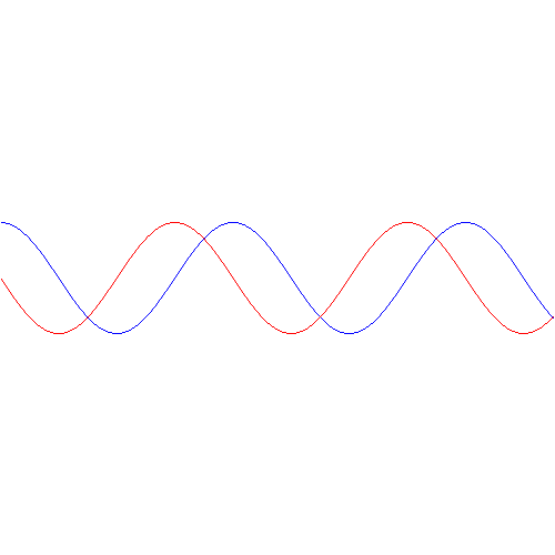
P₁(t) = |C₁(t)|² = cos²[(A/ħ)·t]
P₂(t) = |C₂(t)|²= sin²[(A/ħ)·t]

[Remember: the absolute square of i and −i is |i|²= +√1²= +1 and |−i|²= (−1)²|i|²= +1 respectively, so the i and −i in the two C₂(t) formulas disappear.]

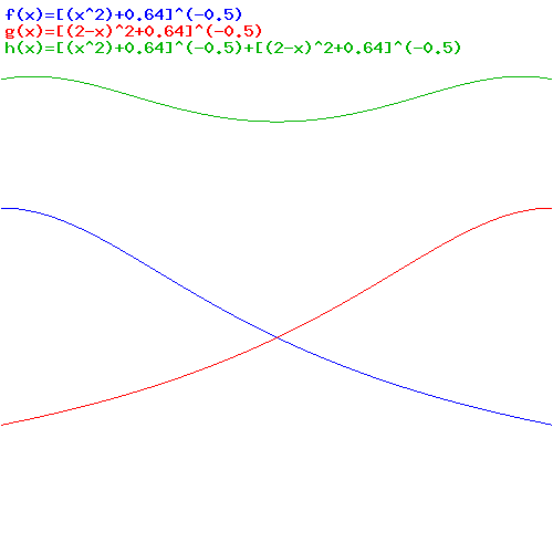
You’ll remember the graph:

Of course, you’ll say: that plus or minus sign in front of C₂(t) should matter somehow, doesn’t it? Well… Think about it. Taking the absolute square of some complex number – or some complex function , in this case! – amounts to multiplying it with its complex conjugate. Because the complex conjugate of a product is the product of the complex conjugates, it’s easy to see what happens: the e^{−(i/ħ)·E₀·t} factor in C₁(t) = e^{−(i/ħ)·E₀·t}·cos[(A/ħ)·t] and C₂(t) = ±i·e^{−(i/ħ)·E₀·t}·sin[(A/ħ)·t] gets multiplied by e^{+(i/ħ)·E₀·t} and, hence, doesn’t matter: e^{−(i/ħ)·E₀·t}·e^{+(i/ħ)·E₀·t} = e⁰= 1. The cosine factor in C₁(t) = e^{−(i/ħ)·E₀·t}·cos[(A/ħ)·t] is real, and so its complex conjugate is the same. Now, the ±i·sin[(A/ħ)·t] factor in C₂(t) = ±i·e^{−(i/ħ)·E₀·t}·sin[(A/ħ)·t] is a pure imaginary number, and so its complex conjugate is its opposite. For some reason, we’ll find similar solutions for all of the situations we’ll describe below: the factor determining the probability will either be real or, else, a pure imaginary number. Hence, from a math point of view, it really doesn’t matter if we take +A or −A for or real factor for those H₁₂and H₂₁ coefficients. We just need to be consistent in our choice, and I must assume that, in order to be consistent, Feynman likes to think of our nitrogen atom borrowing some energy from the system and, hence, temporarily reducing its energy by an amount that’s equal to −A. If you have a better interpretation, please do let me know! 🙂

OK. We’re done with this section… Except… Well… I have to show you how we got those C₁(t) and C₁(t) functions, no? Let me copy Feynman here:

Note that the ‘trick’ involving the addition and subtraction of the differential equations is a trick we’ll use quite often, so please do have a look at it. As for the value of the a and b coefficients – which, as you can see, we’ve equated to 1 in our solutions for C₁(t) and C₁(t) – we get those because of the following starting condition: we assume that at t = 0, the molecule will be in state 1. Hence, we assume C₁(0) = 1 and C₂(0) = 0. In other words: we assume that we start out on that P₁(t) curve in that graph with the probability functions above, so the C₁(0) = 1 and C₂(0) = 0 starting condition is equivalent to P₁(0) = 1 and P₁(0) = 0. Plugging that in gives us a/2 + b/2 = 1 and a/2 − b/2 = 0, which is possible only if a = b = 1.

Of course, you’ll say: what if we’d choose to start out with state 2, so our starting condition is P₁(0) = 0 and P₁(0) = 1? Then a = 1 and b = −1, and we get the solution we got when equating H₁₂and H₂₁ with +A, rather than with −A. So you can think about that symmetry once again: when we’re in free space, then it’s quite arbitrary what we call ‘up’ or ‘down’.

So… Well… That’s all great. I should, perhaps, just add one more note, and that’s on that A/ħ value. We calculated it in the previous post, because we wanted to actually calculate the period of those P₁(t) and P₂(t) functions. Because we’re talking the square of a cosine and a sine respectively, the period is equal to π, rather than 2π, so we wrote: (A/ħ)·T = π ⇔ T = π·ħ/A. Now, the separation between the two energy levels E₀+ A and E₀− A, so that’s 2A, has been measured as being equal, more or less, to 2A ≈ 10⁻⁴eV.

How does one measure that? As mentioned above, I’ll show you, in a moment, that, when applying some external field, the plus and minus sign do matter, and the separation between those two energy levels E₀+ A and E₀− A will effectively represent something physical. More in particular, we’ll have transitions from one energy level to another and that corresponds to electromagnetic radiation being emitted or absorbed, and so there’s a relation between the energy and the frequency of that radiation. To be precise, we can write 2A = h·f₀. The frequency of the radiation that’s being absorbed or emitted is 23.79 GHz, which corresponds to microwave radiation with a wavelength of λ = c/f₀ = 1.26 cm. Hence, 2·A ≈ 25×10⁹ Hz times 4×10⁻¹⁵ eV·s = 10⁻⁴eV, indeed, and, therefore, we can write: T = π·ħ/A ≈ 3.14 × 6.6×10⁻¹⁶eV·s divided by 0.5×10⁻⁴eV, so that’s 40×10⁻¹²seconds = 40 picoseconds. That’s 40 trillionths of a seconds. So that’s very short, and surely much shorter than the time that’s associated with, say, a freely emitting sodium atom, which is of the order of 3.2×10⁻⁸seconds. You may think that makes sense, because the photon energy is so much lower: a sodium light photon is associated with an energy equal to E = h·f = 500×10¹² Hz times 4×10⁻¹⁵ eV·s = 2 eV, so that’s 20,000 times 10⁻⁴eV.

There’s a funny thing, however. An oscillation of a frequency of 500 tera-hertz that lasts 3.2×10⁻⁸seconds is equivalent to 500×10¹² Hz times 3.2×10⁻⁸s ≈ 16 million cycles. However, an oscillation of a frequency of 23.97 giga-hertz that only lasts 40×10⁻¹²seconds is equivalent to 23.97×10⁹ Hz times 40×10⁻¹²s ≈ 1000×10⁻³= 1 ! One cycle only? We’re surely not talking resonance here!

So… Well… I am just flagging it here. We’ll have to do some more thinking about that later. [I’ve added an addendum that may or may not help us in this regard. :-)]

The two-state system in a field

As mentioned above, when there is no external force field, we define the ‘up’ or ‘down’ direction of the nitrogen atom was defined with regard to its its spin around its axis of symmetry, so with regard to the molecule itself. However, when we apply an external electromagnetic field, as shown below, we do have some external reference frame.

Now, the external reference frame – i.e. the physics of the situation, really – may make it more convenient to define the whole system using another set of base states, which we’ll refer to as I and II, rather than 1 and 2. Indeed, you’ve seen the picture below: it shows a state selector, or a filter as we called it. In this case, there’s a filtering according to whether our ammonia molecule is in state I or, alternatively, state II. It’s like a Stern-Gerlach apparatus splitting an electron beam according to the spin state of the electrons, which is ‘up’ or ‘down’ too, but in a totally different way than our ammonia molecule. Indeed, the ‘up’ and ‘down’ spin of an electron has to do with its magnetic moment and its angular momentum. However, there are a lot of similarities here, and so you may want to compare the two situations indeed, i.e. the electron beam in an inhomogeneous magnetic field versus the ammonia beam in an inhomogeneous electric field.

Now, when reading Feynman, as he walks us through the relevant Lecture on all of this, you get the impression that it’s the I and II states only that have some kind of physical or geometric interpretation. That’s not the case. Of course, the diagram of the state selector above makes it very obvious that these new I and II base states make very much sense in regard to the orientation of the field, i.e. with regard to external space, rather than with respect to the position of our nitrogen atom vis-á-vis the hydrogens. But… Well… Look at the image below: the direction of the field (which we denote by ε because we’ve been using the E for energy) obviously matters when defining the old ‘up’ and ‘down’ states of our nitrogen atom too!

In other words, our previous | 1 〉 and | 2 〉 base states acquire a new meaning too: it obviously matters whether or not the electric dipole moment of the molecule is in the same or, conversely, in the opposite direction of the field. To be precise, the presence of the electromagnetic field suddenly gives the energy levels that we’d associate with these two states a very different physical interpretation.

Indeed, from the illustration above, it’s easy to see that the electric dipole moment of this particular molecule in state 1 is in the opposite direction and, therefore, temporarily ignoring the amplitude to flip over (so we do not think of A for just a brief little moment), the energy that we’d associate with state 1 would be equal to E₀+ με. Likewise, the energy we’d associate with state 2 is equal to E₀− με. Indeed, you’ll remember that the (potential) energy of an electric dipole is equal to the vector dot product of the electric dipole moment μ and the field vector ε, but with a minus sign in front so as to get the sign for the energy righ. So the energy is equal to −μ·ε = −|μ|·|ε|·cosθ, with θ the angle between both vectors. Now, the illustration above makes it clear that state 1 and 2 are defined for θ = π and θ = 0 respectively. [And, yes! Please do note that state 1 is the highest energy level, because it’s associated with the highest potential energy: the electric dipole moment μ of our ammonia molecule will – obviously! – want to align itself with the electric field ε ! Just think of what it would imply to turn the molecule in the field!]

Therefore, using the same hunches as the ones we used in the free space example, Feynman suggests that, when some external electric field is involved, we should use the following Hamiltonian matrix:

So we’ll need to solve a similar set of differential equations with this Hamiltonian now. We’ll do that later and, as mentioned above, it will be more convenient to switch to another set of base states, or another ‘representation’ as it’s referred to. But… Well… Let’s not get too much ahead of ourselves: I’ll say something about that before we’ll start solving the thing, but let’s first look at that Hamiltonian once more.

When I say that Feynman uses the same clues here, then… Well.. That’s true and not true. You should note that the diagonal elements in the Hamiltonian above are not the same: E₀+ με ≠ E₀+ με. So we’ve lost that symmetry of free space which, from a math point of view, was reflected in those identical H₁₁= H₂₂= E₀coefficients.

That should be obvious from what I write above: state 1 and state 2 are no longer those 1 and 2 states we described when looking at the molecule in free space. Indeed, the | 1 〉 and | 2 〉 states are still ‘up’ or ‘down’, but the illustration above also makes it clear we’re defining state 1 and state 2 not only with respect to the molecule’s spin around its own axis of symmetry but also vis-á-vis some direction in space. To be precise, we’re defining state 1 and state 2 here with respect to the direction of the electric field ε. Now that makes a really big difference in terms of interpreting what’s going on.

In fact, the ‘splitting’ of the energy levels because of that amplitude A is now something physical too, i.e. something that goes beyond just modeling the uncertainty involved. In fact, we’ll find it convenient to distinguish two new energy levels, which we’ll write as E_I= E₀+ A and E_II= E₀− A respectively. They are, of course, related to those new base states | I 〉 and | II 〉 that we’ll want to use. So the E₀+ A and E₀− A energy levels themselves will acquire some physical meaning, and especially the separation between them, i.e. the value of 2A. Indeed, E_I= E₀+ A and E_II= E₀− A will effectively represent an ‘upper’ and a ‘lower’ energy level respectively.

But, again, I am getting ahead of myself. Let’s first, as part of working towards a solution for our equations, look at what happens if and when we’d switch to another representation indeed.

Switching to another representation

Let me remind you of what I wrote in my post on quantum math in this regard. The actual state of our ammonia molecule – or any quantum-mechanical system really – is always to be described in terms of a set of base states. For example, if we have two possible base states only, we’ll write:

| φ 〉 = | 1 〉 C₁ + | 2 〉 C₂

You’ll say: why? Our molecule is obviously always in either state 1 or state 2, isn’t it? Well… Yes and no. That’s the mystery of quantum mechanics: it is and it isn’t. As long as we don’t measure it, there is an amplitude for it to be in state 1 and an amplitude for it to be in state 2. So we can only make sense of its state by actually calculating 〈 1 | φ 〉 and 〈 2 | φ 〉 which, unsurprisingly are equal to 〈 1 | φ 〉 = 〈 1 | 1 〉 C₁ + 〈 1 | 2 〉 C₂ = C₁(t) and 〈 2 | φ 〉 = 〈 2 | 1 〉 C₁ + 〈 2 | 2 〉 C₂ = C₂(t) respectively, and so these two functions give us the probabilities P₁(t) and P₂(t) respectively. So that’s Schrödinger’s cat really: the cat is dead or alive, but we don’t know until we open the box, and we only have a probability function – so we can say that it’s probably dead or probably alive, depending on the odds – as long as we do not open the box. It’s as simple as that.

Now, the ‘dead’ and ‘alive’ condition are, obviously, the ‘base states’ in Schrödinger’s rather famous example, and we can write them as | DEAD 〉 and | ALIVE 〉 you’d agree it would be difficult to find another representation. For example, it doesn’t make much sense to say that we’ve rotated the two base states over 90 degrees and we now have two new states equal to (1/√2)·| DEAD 〉 – (1/√2)·| ALIVE 〉 and (1/√2)·| DEAD 〉 + (1/√2)·| ALIVE 〉 respectively. There’s no direction in space in regard to which we’re defining those two base states: dead is dead, and alive is alive.

The situation really resembles our ammonia molecule in free space: there’s no external reference against which to define the base states. However, as soon as some external field is involved, we do have a direction in space and, as mentioned above, our base states are now defined with respect to a particular orientation in space. That implies two things. The first is that we should no longer say that our molecule will always be in either state 1 or state 2. There’s no reason for it to be perfectly aligned with or against the field. Its orientation can be anything really, and so its state is likely to be some combination of those two pure base states | 1 〉 and | 2 〉.

The second thing is that we may choose another set of base states, and specify the very same state in terms of the new base states. So, assuming we choose some other set of base states | I 〉 and | II 〉, we can write the very same state | φ 〉 = | 1 〉 C₁ + | 2 〉 C₂as:

| φ 〉 = | I 〉 C_I + | II 〉 C_II

It’s really like what you learned about vectors in high school: one can go from one set of base vectors to another by a transformation, such as, for example, a rotation, or a translation. It’s just that, just like in high school, we need some direction in regard to which we define our rotation or our translation.

For state vectors, I showed how a rotation of base states worked in one of my posts on two-state systems. To be specific, we had the following relation between the two representations:

The (1/√2) factor is there because of the normalization condition, and the two-by-two matrix equals the transformation matrix for a rotation of a state filtering apparatus about the y-axis, over an angle equal to (minus) 90 degrees, which we wrote as:

The y-axis? What y-axis? What state filtering apparatus? Just relax. Think about what you’ve learned already. The orientations are shown below: the S apparatus separates ‘up’ and ‘down’ states along the z-axis, while the T-apparatus does so along an axis that is tilted, about the y-axis, over an angle equal to α, or φ, as it’s written in the table above.

Of course, we don’t really introduce an apparatus at this or that angle. We just introduced an electromagnetic field, which re-defined our | 1 〉 and | 2 〉 base states and, therefore, through the rotational transformation matrix, also defines our | I 〉 and | II 〉 base states.

[…] You may have lost me by now, and so then you’ll want to skip to the next section. That’s fine. Just remember that the representations in terms of | I 〉 and | II 〉 base states or in terms of | 1 〉 and | 2 〉 base states are mathematically equivalent. Having said that, if you’re reading this post, and you want to understand it, truly (because you want to truly understand quantum mechanics), then you should try to stick with me here. 🙂 Indeed, there’s a zillion things you could think about right now, but you should stick to the math now. Using that transformation matrix, we can relate the C_Iand C_IIcoefficients in the | φ 〉 = | I 〉 C_I + | II 〉 C_II expression to the C_Iand C_IIcoefficients in the | φ 〉 = | 1 〉 C₁ + | 2 〉 C₂ expression. Indeed, we wrote:

C_I= 〈 I | ψ 〉 = (1/√2)·(C₁− C₂)
C_II= 〈 II | ψ 〉 = (1/√2)·(C₁+ C₂)

That’s exactly the same as writing:

OK. […] Waw! You just took a huge leap, because we can now compare the two sets of differential equations:

They’re mathematically equivalent, but the mathematical behavior of the functions involved is very different. Indeed, unlike the C₁(t) and C₂(t) amplitudes, we find that the C_I(t) and C_II(t) amplitudes are stationary, i.e. the associated probabilities – which we find by taking the absolute square of the amplitudes, as usual – do not vary in time. To be precise, if you write it all out and simplify, you’ll find that the C_I(t) and C_II(t) amplitudes are equal to:

C_I(t) = 〈 I | ψ 〉 = (1/√2)·(C₁− C₂) = (1/√2)·e^{−(i/ħ)·(E₀+ A)·t} = (1/√2)·e^{−(i/ħ)·E_I·t}
C_II(t) = 〈 II | ψ 〉 = (1/√2)·(C₁+ C₂) = (1/√2)·e^{−(i/ħ)·(E₀− A)·t}= (1/√2)·e^{−(i/ħ)·E_II·t}

As the absolute square of the exponential is equal to one, the associated probabilities, i.e. |C_I(t)|² and |C_II(t)|², are, quite simply, equal to |1/√2|² = 1/2. Now, it is very tempting to say that this means that our ammonia molecule has an equal chance to be in state I or state II. In fact, while I may have said something like that in my previous posts, that’s not how one should interpret this. The chance of our molecule being exactly in state I or state II, or in state 1 or state 2 is varying with time, with the probability being ‘dumped’ from one state to the other all of the time.

I mean… The electric dipole moment can point in any direction, really. So saying that our molecule has a 50/50 chance of being in state 1 or state 2 makes no sense. Likewise, saying that our molecule has a 50/50 chance of being in state I or state II makes no sense either. Indeed, the state of our molecule is specified by the | φ 〉 = | I 〉 C_I + | II 〉 C_II= | 1 〉 C₁ + | 2 〉 C₂equations, and neither of these two expressions is a stationary state. They mix two frequencies, because they mix two energy levels.

Having said that, we’re talking quantum mechanics here and, therefore, an external inhomogeneous electric field will effectively split the ammonia molecules according to their state. The situation is really like what a Stern-Gerlach apparatus does to a beam of electrons: it will split the beam according to the electron’s spin, which is either ‘up’ or, else, ‘down’, as shown in the graph below:

The graph for our ammonia molecule, shown below, is very similar. The vertical axis measures the same: energy. And the horizontal axis measures με, which increases with the strength of the electric field ε. So we see a similar ‘splitting’ of the energy of the molecule in an external electric field.

How should we explain this? It is very tempting to think that the presence of an external force field causes the electrons, or the ammonia molecule, to ‘snap into’ one of the two possible states, which are referred to as state I and state II respectively in the illustration of the ammonia state selector below. But… Well… Here we’re entering the murky waters of actually interpreting quantum mechanics, for which (a) we have no time, and (b) we are not qualified. So you should just believe, or take for granted, what’s being shown here: an inhomogeneous electric field will split our ammonia beam according to their state, which we define as I and II respectively, and which are associated with the energy E₀+ A and E₀− A respectively.

electric field

As mentioned above, you should note that these two states are stationary. The Hamiltonian equations which, as they always do, describe the dynamics of this system, imply that the amplitude to go from state I to state II, or vice versa, is zero. To make sure you ‘get’ that, I reproduce the associated Hamiltonian matrix once again:

Of course, that will change when we start our analysis of what’s happening in the maser. Indeed, we will have some non-zero H_I,II and H_II,Iamplitudes in the resonant cavity of our ammonia maser, in which we’ll have an oscillating electric field and, as a result, induced transitions from state I to II and vice versa. However, that’s for later. While I’ll quickly insert the full picture diagram below, you should, for the moment, just think about those two stationary states and those two zeroes. 🙂

Capito? If not… Well… Start reading this post again, I’d say. 🙂

Intermezzo: on approximations

At this point, I need to say a few things about all of the approximations involved, because it can be quite confusing indeed. So let’s take a closer look at those energy levels and the related Hamiltonian coefficients. In fact, in his Lectures, Feynman shows us that we can always have a general solution for the Hamiltonian equations describing a two-state system whenever we have constant Hamiltonian coefficients. That general solution – which, mind you, is derived assuming Hamiltonian coefficients that do not depend on time – can always be written in terms of two stationary base states, i.e. states with a definite energy and, hence, a constant probability. The equations, and the two definite energy levels are:

That yields the following values for the energy levels for the stationary states:

Now, that’s very different from the E_I= E₀+ A and E_II= E₀− A energy levels for those stationary states we had defined in the previous section: those stationary states had no square root, and no μ²ε², in their energy. In fact, that sort of answers the question: if there’s no external field, then that μ²ε² factor is zero, and the square root in the expression becomes ±√A²= ±A. So then we’re back to our E_I= E₀+ A and E_II= E₀− A formulas. The whole point, however, is that we will actually have an electric field in that cavity. Moreover, it’s going to be a field that varies in time, which we’ll write:

Now, part of the confusion in Feynman’s approach is that he constantly switches between representing the system in terms of the I and II base states and the 1 and 2 base states respectively. For a good understanding, we should compare with our original representation of the dynamics in free space, for which the Hamiltonian was the following one:

That matrix can easily be related to the new one we’re going to have to solve, which is equal to:

The interpretation is easy if we look at that illustration again:

If the direction of the electric dipole moment is opposite to the direction ε, then the associated energy is equal to −μ·ε = −μ·ε = −|μ|·|ε|·cosθ = −μ·ε·cos(π) = +με. Conversely, for state 2, we find −μ·ε·cos(0) = −με for the energy that’s associated with the dipole moment. You can and should think about the physics involved here, because they make sense! Thinking of amplitudes, you should note that the +με and −με terms effectively change the H₁₁ and H₂₂ coefficients, so they change the amplitude to stay in state 1 or state 2 respectively. That, of course, will have an impact on the associated probabilities, and so that’s why we’re talking of induced transitions now.

Having said that, the Hamiltonian matrix above keeps the −A for H₁₂ and H₂₁, so the matrix captures spontaneous transitions too!

Still… You may wonder why Feynman doesn’t use those E_Iand E_IIformulas with the square root because that would give us some exact solution, wouldn’t it? The answer to that question is: maybe it would, but would you know how to solve those equations? We’ll have a varying field, remember? So our Hamiltonian H₁₁ and H₂₂ coefficients will no longer be constant, but time-dependent. As you’re going to see, it takes Feynman three pages to solve the whole thing using the +με and −με approximation. So just imagine how complicated it would be using that square root expression! [By the way, do have a look at those asymptotic curves in that illustration showing the splitting of energy levels above, so you see how that approximation looks like.]

So that’s the real answer: we need to simplify somehow, so as to get any solutions at all!

Of course, it’s all quite confusing because, after Feynman first notes that, for strong fields, the A² in that square root is small as compared to μ²ε², thereby justifying the use of the simplified E_I= E₀+ με = H₁₁ and E_II= E₀− με = H₂₂ coefficients, he continues and bluntly uses the very same square root expression to explain how that state selector works, saying that the electric field in the state selector will be rather weak and, hence, that με will be much smaller than A, so one can use the following approximation for the square root in the expressions above:

The energy expressions then reduce to:

And then we can calculate the force on the molecules as:

So the electric field in the state selector is weak, but the electric field in the cavity is supposed to be strong, and so… Well… That’s it, really. The bottom line is that we’ve a beam of ammonia molecules that are all in state I, and it’s what happens with that beam then, that is being described by our new set of differential equations:

Solving the equations

As all molecules in our ammonia beam are described in terms of the | I 〉 and | II 〉 base states – as evidenced by the fact that we say all molecules that enter the cavity are state I – we need to switch to that representation. We do that by using that transformation above, so we write:

C_I= 〈 I | ψ 〉 = (1/√2)·(C₁− C₂)
C_II= 〈 II | ψ 〉 = (1/√2)·(C₁+ C₂)

Keeping these ‘definitions’ of C_Iand C_IIin mind, you should then add the two differential equations, divide the result by the square root of 2, and you should get the following new equation:

Please! Do it and verify the result! You want to learn something here, no? 🙂

Likewise, subtracting the two differential equations, we get:

We can re-write this as:

Now, the problem is that the Hamiltonian constants here are not constant. To be precise, the electric field ε varies in time. We wrote:

So H_I,IIand H_II,I, which are equal to με, are not constant: we’ve got Hamiltonian coefficients that are a function of time themselves. […] So… Well… We just need to get on with it and try to finally solve this thing. Let me just copy Feynman as he grinds through this:

This is only the first step in the process. Feynman just takes two trial functions, which are really similar to the very general C₁= a·e^{–(i/ħ)·H₁₁·t}function we presented when only one equation was involved, or – if you prefer a set of two equations – those C_I(t) = a·e^{−(i/ħ)·E_I·t}and C_I(t) = b·e^{−(i/ħ)·E_II·}^tequations above. The difference is that the coefficients in front, i.e. γ_I and γ_II are not some (complex) constant, but functions of time themselves. The next step in the derivation is as follows:

One needs to do a bit of gymnastics here as well to follow what’s going on, but please do check and you’ll see it works. Feynman derives another set of differential equations here, and they specify these γ_I = γ_I(t) and γ_II = γ_II(t) functions. These equations are written in terms of the frequency of the field, i.e. ω, and the resonant frequency ω₀, which we mentioned above when calculating that 23.79 GHz frequency from the 2A = h·f₀ equation. So ω₀ is the same molecular resonance frequency but expressed as an angular frequency, so ω₀ = f₀/2π = ħ/2A. He then proceeds to simplify, using assumptions one should check. He then continues:

That gives us what we presented in the previous post:

So… Well… What to say? I explained those probability functions in my previous post, indeed. We’ve got two probabilities here:

P_I= cos²[(με₀/ħ)·t]
P_II= sin²[(με₀/ħ)·t]

So that’s just like the P₁= cos²[(A/ħ)·t] and P₂= sin²[(A/ħ)·t] probabilities we found for spontaneous transitions. But so here we are talking induced transitions.

As you can see, the frequency and, hence, the period, depend on the strength, or magnitude, of the electric field, i.e. the ε₀constant in the ε = 2ε₀cos(ω·t) expression. The natural unit for measuring time would be the period once again, which we can easily calculate as (με₀/ħ)·T = π ⇔ T = π·ħ/με₀.

Now, we had that T = (π·ħ)/(2A) expression above, which allowed us to calculate the period of the spontaneous transition frequency, which we found was like 40 picoseconds, i.e. 40×10⁻¹²seconds. Now, the T = (π·ħ)/(2με₀) is very similar, it allows us to calculate the expected, average, or mean time for an induced transition. In fact, if we write T_induced = (π·ħ)/(2με₀) and T_spontaneous = (π·ħ)/(2A), then we can take ratio to find:

T_induced/T_spontaneous = [(π·ħ)/(2με₀)]/[(π·ħ)/(2A)] = A/με₀

This A/με₀ratio is greater than one, so T_induced/T_spontaneous is greater than one, which, in turn, means that the presence of our electric field – which, let me remind you, dances to the beat of the resonant frequency – causes a slower transition than we would have had if the oscillating electric field were not present.

But – Hey! – that’s the wrong comparison! Remember all molecules enter in a stationary state, as they’ve been selected so as to ensure they’re in state I. So there is no such thing as a spontaneous transition frequency here! They’re all polarized, so to speak, and they would remain that way if there was no field in the cavity. So if there was no oscillating electric field, they would never transition. Nothing would happen! Well… In terms of our particular set of base states, of course! Why? Well… Look at the Hamiltonian coefficients H_I,II= H_II,I= με: these coefficients are zero if ε is zero. So… Well… That says it all.

So that‘s what it’s all about: induced emission and, as I explained in my previous post, because all molecules enter in state I, i.e. the upper energy state, literally, they all ‘dump’ a net amount of energy equal to 2A into the cavity at the occasion of their first transition. The molecules then keep dancing, of course, and so they absorb and emit the same amount as they go through the cavity, but… Well… We’ve got a net contribution here, which is not only enough to maintain the cavity oscillations, but actually also provides a small excess of power that can be drawn from the cavity as microwave radiation of the same frequency.

As Feynman notes, an exact description of what actually happens requires an understanding of the quantum mechanics of the field in the cavity, i.e. quantum field theory, which I haven’t studied yet. But… Well… That’s for later, I guess. 🙂

Post scriptum: The sheer length of this post shows we’re not doing something that’s easy here. Frankly, I feel the whole analysis is still quite obscure, in the sense that – despite looking at this thing again and again – it’s hard to sort of interpret what’s going on, in a physical sense that is. But perhaps one shouldn’t try that. I’ve quoted Feynman’s view on how easy or how difficult it is to ‘understand’ quantum mechanics a couple of times already, so let me do it once more:

So… Well… I’ll grind through the remaining Lectures now – I am halfway through Volume III now – and then re-visit all of this. Despite Feynman’s warning, I want to understand it the way I like to, even if I don’t quite know what way that is right now. 🙂

Addendum: As for those cycles and periods, I noted a couple of times already that the Planck-Einstein equation E = h·f can usefully be re-written as E/f = h, as it gives a physical interpretation to the value of the Planck constant. In fact, I said h is the energy that’s associated with one cycle, regardless of the frequency of the radiation involved. Indeed, the energy of a photon divided by the number of cycles per second, should give us the energy per cycle, no?

Well… Yes and no. Planck’s constant h and the frequency f are both expressed referencing the time unit. However, if we say that a sodium atom emits one photon only as its electron transitions from a higher energy level to a lower one, and if we say that involves a decay time of the order of 3.2×10⁻⁸seconds, then what we’re saying really is that a sodium light photon will ‘pack’ like 16 million cycles, which is what we get when we multiply the number of cycles per second (i.e. the mentioned frequency of 500×10¹²Hz) by the decay time (i.e. 3.2×10⁻⁸seconds): (500×10¹²Hz)·(3.2×10⁻⁸s) = 16 ×10⁶cycles, indeed. So the energy per cycle is 2.068 eV (i.e. the photon energy) divided by 16×10⁶, so that’s 0.129×10⁻⁶eV. Unsurprisingly, that’s what we get when we we divide h by 3.2×10⁻⁸s: (4.13567×10⁻¹⁵)/(3.2×10⁻⁸s) = 1.29×10⁻⁷eV. We’re just putting some values in to the E/(f·T) = h/T equation here.

The logic for that 2A = h·f₀ is the same. The frequency of the radiation that’s being absorbed or emitted is 23.79 GHz, so the photon energy is (23.97×10⁹ Hz)·(4.13567×10⁻¹⁵ eV·s) ≈ 1×10⁻⁴eV. Now, we calculated the transition period T as T = π·ħ/A ≈ (π·6.626×10⁻¹⁶eV·s)/(0.5×10⁻⁴eV) ≈ 41.6×10⁻¹²seconds. Now, an oscillation of a frequency of 23.97 giga-hertz that only lasts 41.6×10⁻¹²seconds is an oscillation of one cycle only. The consequence is that, when we continue this style of reasoning, we’d have a photon that packs all of its energy into one cycle!

Let’s think about what this implies in terms of the density in space. The wavelength of our microwave radiation is 1.25×10⁻²m, so we’ve got a ‘density’ of 1×10⁻⁴eV/1.25×10⁻²m = 0.8×10⁻²eV/m = 0.008 eV/m. The wavelength of our sodium light is 0.6×10⁻⁶m, so we get a ‘density’ of 1.29×10⁻⁷eV/0.6×10⁻⁶m = 2.15×10⁻¹eV/m = 0.215 eV/m. So the energy ‘density’ of our sodium light is 26.875 times that of our microwave radiation. 🙂

Frankly, I am not quite sure if calculations like this make much sense. In fact, when talking about energy densities, I should review my posts on the Poynting vector. However, they may help you think things through. 🙂

Quantum math revisited

It’s probably good to review the concepts we’ve learned so far. Let’s start with the foundation of all of our math, i.e. the concept of the state, or the state vector. [The difference between the two concepts is subtle but real. I’ll come back to it.]

State vectors and base states

We used Dirac’s bra-ket notation to denote a state vector, in general, as | ψ 〉. The obvious question is: what is this thing? We called it a vector because we use it like a vector: we multiply it with some number, and then add it to some other vector. So that’s just what you did in high school, when you learned about real vector spaces. In this regard, it is good to remind you of the definition of a vector space. To put it simply, it is is a collection of objects called vectors, which may be added together, and multiplied by numbers. So we have two things here: the ‘objects’, and the ‘numbers’. That’s why we’d say that we have some vector space over a field of numbers. [The term ‘field’ just refers to an algebraic structure, so we can add and multiply and what have you.] Of course, what it means to ‘add’ two ‘objects’, and what it means to ‘multiply’ an object with a number, depends on the type of objects and, unsurprisingly, the type of numbers.

Huh? The type of number?! A number is a number, no?

No, hombre, no! We’ve got natural numbers, rational numbers, real numbers, complex numbers—and you’ve probably heard of quaternions too – and, hence, ‘multiplying’ a ‘number’ with ‘something else’ can mean very different things. At the same time, the general idea is the general idea, so that’s the same, indeed. 🙂 When using real numbers and the kind of vectors you are used to (i.e. Euclidean vectors), then the multiplication amounts to a re-scaling of the vector, and so that’s why a real number is often referred to as a scalar. At the same time, anything that can be used to multiply a vector is often referred to as a scalar in math so… Well… Terminology is often quite confusing. In fact, I’ll give you some more examples of confusing terminology in a moment. But let’s first look at our ‘objects’ here, i.e. our ‘vectors’.

I did a post on Euclidean and non-Euclidean vector spaces two years ago, when I started this blog, but state vectors are obviously very different ‘objects’. They don’t resemble the vectors we’re used to. We’re used to so-called polar vectors, aka as real vectors, like the position vector (x or r), or the momentum vector (p = m·v), or the electric field vector (E). We are also familiar with the so-called pseudo-vectors, aka as axial vectors, like angular momentum (L = r×p), or the magnetic dipole moment. [Unlike what you might think, not all vector cross products yield a pseudo-vector. For example, the cross-product of a polar and an axial vector yields a polar vector.] But here we are talking some very different ‘object’. In math, we say that state vectors are elements in a Hilbert space. So a Hilbert space is a vector space but… Well… With special vectors. 🙂

The key to understanding why we’d refer to states as state vectors is the fact that, just like Euclidean vectors, we can uniquely specify any element in a Hilbert space with respect to a set of base states. So it’s really like using Cartesian coordinates in a two- or three-dimensional Euclidean space. The analogy is complete because, even in the absence of a geometrical interpretation, we’ll require those base states to be orthonormal. Let me be explicit on that by reminding you of your high-school classes on vector analysis: you’d choose a set of orthonormal base vectors e₁, e₂, and e₃, and you’d write any vector A as:

A = (A_x, A_y, A_z) = A_x·e₁ + A_y·e₂+ A_z·e₃ with e_i·e_j = 1 if i = j, and e_i·e_j = 0 if i ≠ j

The e_i·e_j = 1 if i = j and e_i·e_j = 0 if i ≠ j condition expresses the orthonormality condition: the base vectors need to be orthogonal unit vectors. We wrote it as e_i·e_j = δ_ijusing the Kronecker delta (δ_ij= 1 if i = j and 0 if i ≠ j). Now, base states in quantum mechanics do not necessarily have a geometrical interpretation. Indeed, although one often can actually associate them with some position or direction in space, the condition of orthonormality applies in the mathematical sense of the word only. Denoting the base states by i = 1, 2,… – or by Roman numerals, like I and II – so as to distinguish them from the Greek ψ or φ symbols we use to denote state vectors in general, we write the orthonormality condition as follows:

〈 i | j 〉 = δ_ij, with δ_ij= δ_jiis equal to 1 if i = j, and zero if i ≠ j

Now, you may grumble and say: that 〈 i | j 〉 bra-ket does not resemble the e_i·e_j product. Well… It does and it doesn’t. I’ll show why in a moment. First note how we uniquely specify state vectors in general in terms of a set of base states. For example, if we have two possible base states only, we’ll write:

| φ 〉 = | 1 〉 C₁ + | 2 〉 C₂

Or, if we chose some other set of base states | I 〉 and | II 〉, we’ll write:

| φ 〉 = | I 〉 C_I + | II 〉 C_II

You should note that the | 1 〉 C₁ term in the | φ 〉 = | 1 〉 C₁ + | 2 〉 C₂ sum is really like the A_x·e₁ product in the A = A_x·e₁ + A_y·e₂+ A_z·e₃ expression. In fact, you may actually write it as C₁·| 1 〉, or just reverse the order and write C₁| 1 〉. However, that’s not common practice and so I won’t do that, except occasionally. So you should look at | 1 〉 C₁ as a product indeed: it’s the product of a base state and a complex number, so it’s really like m·v, or whatever other product of some scalar and some vector, except that we’ve got a complex scalar here. […] Yes, I know the term ‘complex scalar’ doesn’t make sense, but I hope you know what I mean. 🙂

More generally, we write:

Writing our state vector | ψ 〉, | φ 〉 or | χ 〉 like this also defines these coefficients or coordinates C_i. Unlike our state vectors, or our base states, C_iis an actual number. It has to be, of course: it’s the complex number that makes sense of the whole expression. To be precise, C_iis an amplitude, or a wavefunction, i.e. a function depending on both space and time. In our previous posts, we limited the analysis to amplitudes varying in time only, and we’ll continue to do so for a while. However, at some point, you’ll get the full picture.

Now, what about the supposed similarity between the 〈 i | j〉 bra-ket and the e_i·e_j product? Let me invoke what Feynman, tongue-in-cheek as usual, refers to as the Great Law of Quantum Mechanics:

You get this by taking | ψ 〉 out of the | ψ 〉 = ∑| i 〉〈 i | ψ 〉 expression. And, no, don’t say: what nonsense! Because… Well… Dirac’s notation really is that simple and powerful! You just have to read it from right to left. There’s an order to the symbols, unlike what you’re used to in math, because you’re used to operations that are commutative. But I need to move on. The upshot is that we can specify our base states in terms of the base states too. For example, if we have only two base states, let’s say I and II, then we can write:

| I 〉 = ∑| i 〉〈 i | 1 〉 = 1·| I 〉 + 0·| II 〉 and | II 〉 = ∑| i 〉〈 i | II 〉 = 0·| 1 〉 + 0·| II 〉

We can write this using a matrix notation:

Now that is silly, you’ll say. What’s the use of this? It doesn’t tell us anything new, and it also does not show us why we should think of the 〈 i | j 〉 bra-ket and the e_i·e_j product as being similar! Well… Yes and no. Let me show you something else. Let’s assume we’ve got some state χ and φ, which we specify in terms of our chosen set of base states as | χ 〉 = ∑ | i 〉 D_i and | φ 〉 = ∑ | i 〉 C_i respectively. Now, from our post on quantum math, you’ll remember that 〈 χ | i 〉 and 〈 i | χ 〉 are each other’s complex conjugates, so we know that 〈 χ | i 〉 = 〈 i | χ 〉* = D_i*. So if we have all C_i = 〈 i | φ 〉 and all D_i = 〈 i | χ 〉, i.e. the ‘components’ of both states in terms of our base states, then we can calculate 〈 χ | φ 〉 – i.e. the amplitude to go from some state φ to some state χ as:

〈 χ | φ 〉 = ∑〈 χ | i 〉〈 i | φ 〉 =∑ D_i*C_i= ∑ D_i*〈 i | φ 〉

We can now scrap | φ 〉 in this expression – yes, it’s the power of Dirac’s notation once more! – so we get:

Now, we can re-write this using a matrix notation:

[I assumed that we have three base states now, so as to make the example somewhat less obvious. Please note we can never leave one of the base states out when specifying a state vector, so it’s not like the previous example was not complete. I’ll switch from two-state to three-state systems and back again all the time, so as to show the analysis is pretty general. To visualize things, think of the ammonia molecule as an example of a two-state system versus the spin of a proton or an electron as a three-state system, respectively. OK. Let’s get back to the lesson.]

You’ll say: so what? Well… Look at this:

I just combined the notations for 〈 I | and | III 〉. Can you now see the similarity between the the 〈 i | j〉 bra-ket and the e_i·e_j product? It really is the same: you just need to respect the subtleties in regard to writing the 〈 i | and | j 〉 vector, or the e_iand e_j vectors, as a row vector or a column vector respectively.

It doesn’t stop here, of course. When learning about vectors in high school, we also learned that we could go from one set of base vectors to another by a transformation, such as, for example, a rotation, or a translation. We showed how a rotation worked in one of our post on two-state systems, where we wrote:

So we’ve got that transformation matrix, which, of course, isn’t random. To be precise, we got the matrix equation above (note that we’re back to two states only, so as to simplify) because we defined the C_Iand C_IIcoefficients in the | φ 〉 = | I 〉 C_I + | II 〉 C_II = | 1 〉 C₁ + | 2 〉 C₂ expression as follows:

C_I= 〈 I | ψ 〉 = (1/√2)·(C₁− C₂)
C_II= 〈 II | ψ 〉 = (1/√2)·(C₁+ C₂)

The (1/√2) factor is there because of the normalization condition, and the two-by-two matrix equals the transformation matrix for a rotation of a state filtering apparatus about the y-axis, over an angle equal to (minus) 90 degrees, which we wrote as:

I promised I’d say something more about confusing terminology so let me do that here. We call a set of base states a ‘representation‘, and writing a state vector in terms of a set of base states is often referred to as a ‘projection‘ of that state into the base set. Again, we can see it’s sort of a mathematical projection, rather than a geometrical one. But it makes sense. In any case, that’s enough on state vectors and base states.

Let me wrap it up by inserting one more matrix equation, which you should be able to reconstruct yourself:

The only thing we’re doing here is to substitute 〈 χ | and | φ 〉 for ∑ D_j*〈 j | and ∑ | i 〉 C_i respectively. All the rest follows. Finally, I promised I’d tell you the difference between a state and a state vector. It’s subtle and, in practice, the two concepts refer to the same. However, we write a state as a state, like ψ or, if it’s a base state, like I, or ‘up’, or whatever. When we say a state vector, then we think of a set of numbers. It may be a row vector, like the 〈 χ | row vector with the D_i* coefficients, or a column vector, like the | φ 〉 column vector with the D_i* coefficients. But so if we say vector, then we think of a one-dimensional array of numbers, while the state itself is… Well… The state. So that’s some reality in physics. So you might define the state vector as the set of numbers that describes the state. While the difference is subtle, it’s important. It’s also important to note that the 〈 χ | and | χ 〉 state vectors are different too. The former appears as the final state in an amplitude, while the latter describes the starting condition. The former is referred to as a bra in the 〈 χ | φ 〉 bra-ket, while the latter is a ket in the 〈 φ | χ 〉 = 〈 χ | φ 〉* amplitude. 〈 χ | is a row vector equal to ∑ D_i*〈 i |, while | χ 〉 = ∑ D_i| χ 〉. So it’s quite different. More in general, we’d define bras and kets as row and column vectors respectively, so we write:

That makes it clear that a bra next to a ket is to be understood as a matrix multiplication. From what I wrote, it is also obvious that the conjugate transpose (which is also known as the Hermitian conjugate) of a bra is the corresponding ket and vice versa, so we write:

Let me formally define the conjugate or Hermitian transpose here: the conjugate transpose of an m-by-n matrix $A$ $with complex elements is the$ n-by-m matrix A† obtained from $A$ by taking the transpose (so we write the rows as columns and vice versa) and then taking the complex conjugate of each element (i.e. we switch the sign of the imaginary part of the complex number). A† is read as ‘A dagger’, but mathematicians will usually denote it by $A*$ . In fact, there are a lot of equivalent notations, as we can write:

OK. That’s it on this.

One more thing, perhaps. We’ll often have states, or base states, that make sense, in a physical sense, that is. But it’s not always the case: we’ll sometimes use base states that may not represent some situation we’re likely to encounter, but that make sense mathematically. We gave the example of the ‘mathematical’ | I 〉 and | II 〉 base states, versus the ‘physical’ | 1 〉 and | 2 〉 base states, in our post on the ammonia molecule, so I won’t say more about this here. Do keep it in mind though. Sometimes it may feel like nothing makes sense, physically, but it usually does mathematically and, therefore, all usually comes out alright in the end. 🙂 To be precise, what we did there, was to choose base states with a unambiguous, i.e. a definite, energy level. That made our calculations much easier, and the end result was the same, indeed!

So… Well… I’ll let this sink in, and move on to the next topic.

The Hamiltonian operator

In my post on the post on the Hamiltonian, I explained that those C_i and D_i coefficients are usually a function of time, and how they can be determined. To be precise, they’re determined by a set of differential equations (i.e. equations involving a function and the derivative of that function) which we wrote as:

If we have two base states only, then this set of equations can be written as:

Two equations and two functions – C₁= C₁(t) and C₂= C₂(t) – so we should be able to solve this thing, right? Well… No. We don’t know those H_ijcoefficients. As I explained in that post, they also evolve in time, so we should write them as H_ij(t) instead of H_ijtout court, and so it messes the whole thing up. We have two equations and six functions really. Of course, there’s always a way out, but I won’t dwell on that here—not now at least. What I want to do here is look at the Hamiltonian as an operator.

We introduced operators – but not very rigorously – when explaining the Hamiltonian. We did so by ‘expanding’ our 〈 χ | φ 〉 amplitude as follows. We’d say the amplitude to find a ‘thing’ – like a particle, for example, or some system, of particles or other things – in some state χ at the time t = t₂, when it was in some state φ state at the time t = t₁ was equal to:

Now, a formula like this only makes sense because we’re ‘abstracting away’ from the base states, which we need to describe any state. Hence, to actually describe what’s going on, we have to choose some representation and expand this expression as follows:

That looks pretty monstrous, so we should write it all out. Using the matrix notation I introduced above, we can do that – let’s take a practical example with three base states once again – as follows:

Now, this still looks pretty monstrous, but just think of it. We’re just applying that ‘Great Law of Quantum Physics’ here, i.e. | = ∑ | i 〉〈 i | over all base states i. To be precise, we apply it to an 〈 χ | A | φ 〉 expression, and we do so twice, so we get:

Nothing more, nothing less. 🙂 Now, the idea of an operator is the result of being creative: we just drop the 〈 χ | state from the expression above to write:

Yes. I know. That’s a lot to swallow, but you’ll see it makes sense because of the Great Law of Quantum Mechanics:

Just think about it and continue reading when you’re ready. 🙂 The upshot is: we now think of the particle entering some ‘apparatus’ A in the state ϕ and coming out of A in some state ψ or, looking at A as an operator, we can generalize this. As Feynman puts it:

“The symbol A is neither an amplitude, nor a vector; it is a new kind of thing called an operator. It is something which “operates on” a state to produce a new state.”

Back to our Hamiltonian. Let’s go through the same process of ‘abstraction’. Let’s first re-write that ‘Hamiltonian equation’ as follows:

The H_ij(t) are amplitudes indeed, and we can represent them in a 〈 i | H_ij(t) | j 〉 matrix indeed! Now let’s take the first step in our ‘abstraction process’: let’s scrap the 〈 i | bit. We get:

We can, of course, also abstract away from the | j 〉 bit, so we get:

Look at this! The right-hand side of this expression is exactly the same as that A | χ 〉 format we presented when introducing the concept of an operator. [In fact, when I say you should ‘abstract away’ from the | j 〉 bit, then you should think of the ‘Great Law’ and that matrix notation above.] So H is an operator and, therefore, it’s something which operates on a state to produce a new state.

OK. Clear enough. But what’s that ‘state’ on the left-hand side? I’ll just paraphrase Feynman here, who says we should think of it as follows: “The time derivative of the state vector |ψ〉 times iℏ is equal to what you get by (1) operating with the Hamiltonian operator H on each base state, (2) multiplying by the amplitude that ψ is in the state j (i.e. 〈j|ψ〉), and (1) summing over all j.” Alternatively, you can also say: “The time derivative, times iħ, of a state |ψ〉 is equal to what you get if you operate on it with the Hamiltonian.” Of course, that’s true for any state, so we can ‘abstract away’ the |ψ〉 bit too and, putting a little hat (^) over the operator to remind ourselves that it’s an operator (rather than just any matrix), we get the Hamiltonian operator equation:

Now, that’s all nice and great, but the key question, of course, is: what can you do with this? Well… It turns out his Hamiltonian operators is useful to calculate lots of stuff. In the first place, of course, it’s a useful operator in the context of those differential equations describing the dynamics of a quantum-mechanical system. When everything is said and done, those equations are the equivalent, in quantum physics, of the law of motion in classical physics. [And I am not joking here.]

In addition, the Hamiltonian operator also has other uses. The one I should really mention here is that you can calculate the average or expected value (EV[X]) of the energy of a state ψ (i.e. any state, really) by first operating on | ψ 〉 with the Hamiltonian, and then multiplying 〈 ψ | with the result. That sounds a bit complicated, but you’ll understand it when seeing the mathematical expression, which we can write as:

The formula is pretty straightforward. [If you don’t think so, then just write it all out using the matrix notation.] But you may wonder how it works exactly… Well… Sorry. I don’t want to copy all of Feynman here, so I’ll refer you to him on this. In fact, the proof of this formula is actually very straightforward, and so you should be able to get through it with the math you got here. You may even understand Feynman’s illustration of it for the ‘special case’ when base states are, indeed, those mathematically convenient base states with definite energy levels.

Have fun with it! 🙂

Post scriptum on Hilbert spaces:

As mentioned above, our state vectors are actually functions. To be specific, they are wavefunctions, i.e. periodic functions, evolving in space and time, so we usually write them as ψ = ψ(x, t). Our ‘Hilbert space’, i.e. our collection of state vectors, is, therefore, often referred to as a function space. So it’s a set of functions. At the same time, it is a vector space too, because we have those addition and multiplication operations, so our function space has the algebraic structure of a vector space. As you can imagine, there are some mathematical conditions for a space or a set of objects to ‘qualify’ as a Hilbert space, and the epithet itself comes with a lot of interesting properties. One of them is completeness, which is a property that allows us to jot down those differential equations that describe the dynamics of a quantum-mechanical system. However, as you can find whatever you’d need or want to know about those mathematical properties on the Web, I won’t get into it. The important thing here is to understand the concept of a Hilbert space intuitively. I hope this post has helped you in that regard, at least. 🙂

Occam’s Razor

The analysis of a two-state system (i.e. the rather famous example of an ammonia molecule ‘flipping’ its spin direction from ‘up’ to ‘down’, or vice versa) in my previous post is a good opportunity to think about Occam’s Razor once more. What are we doing? What does the math tell us?

In the example we chose, we didn’t need to worry about space. It was all about time: an evolving state over time. We also knew the answers we wanted to get: if there is some probability for the system to ‘flip’ from one state to another, we know it will, at some point in time. We also want probabilities to add up to one, so we knew the graph below had to be the result we would find: if our molecule can be in two states only, and it starts of in one, then the probability that it will remain in that state will gradually decline, while the probability that it flips into the other state will gradually increase, which is what is depicted below.

However, the graph above is only a Platonic idea: we don’t bother to actually verify what state the molecule is in. If we did, we’d have to ‘re-set’ our t = 0 point, and start all over again. The wavefunction would collapse, as they say, because we’ve made a measurement. However, having said that, yes, in the physicist’s Platonic world of ideas, the probability functions above make perfect sense. They are beautiful. You should note, for example, that P₁ (i.e. the probability to be in state 1) and P₂ (i.e. the probability to be in state 2) add up to 1 all of the time, so we don’t need to integrate over a cycle or something: so it’s all perfect!

These probability functions are based on ideas that are even more Platonic: interfering amplitudes. Let me explain.

Quantum physics is based on the idea that these probabilities are determined by some wavefunction, a complex-valued amplitude that varies in time and space. It’s a two-dimensional thing, and then it’s not. It’s two-dimensional because it combines a sine and cosine, i.e. a real and an imaginary part, but the argument of the sine and the cosine is the same, and the sine and cosine are the same function, except for a phase shift equal to π. We write:

a·e^−iθ= a·cos(θ) – a·sin(−θ) = a·cosθ – a·sinθ

The minus sign is there because it turns out that Nature measures angles, i.e. our phase, clockwise, rather than counterclockwise, so that’s not as per our mathematical convention. But that’s a minor detail, really. [It should give you some food for thought, though.] For the rest, the related graph is as simple as the formula:

Now, the phase of this wavefunction is written as θ = (ω·t − k ∙x). Hence, ω determines how this wavefunction varies in time, and the wavevector k tells us how this wave varies in space. The young Frenchman Comte Louis de Broglie noted the mathematical similarity between the ω·t − k ∙x expression and Einstein’s four-vector product p_μx_μ= E·t − p∙x, which remains invariant under a Lorentz transformation. He also understood that the Planck-Einstein relation E = ħ·ω actually defines the energy unit and, therefore, that any frequency, any oscillation really, in space or in time, is to be expressed in terms of ħ.

[To be precise, the fundamental quantum of energy is h = ħ·2π, because that’s the energy of one cycle. To illustrate the point, think of the Planck-Einstein relation. It gives us the energy of a photon with frequency f: E_γ = h·f. If we re-write this equation as E_γ/f = h, and we do a dimensional analysis, we get: h = E_γ/f ⇔ 6.626×10⁻³⁴ joule·second = [x joule]/[f cycles per second] ⇔ h = 6.626×10⁻³⁴ joule per cycle. It’s only because we are expressing ω and k as angular frequencies (i.e. in radians per second or per meter, rather than in cycles per second or per meter) that we have to think of ħ = h/2π rather than h.]

Louis de Broglie connected the dots between some other equations too. He was fully familiar with the equations determining the phase and group velocity of composite waves, or a wavetrain that actually might represent a wavicle traveling through spacetime. In short, he boldly equated ω with ω = E/ħ and k with k = p/ħ, and all came out alright. It made perfect sense!

I’ve written enough about this. What I want to write about here is how this also makes for the situation on hand: a simple two-state system that depends on time only. So its phase is θ = ω·t = E₀/ħ. What’s E₀? It is the total energy of the system, including the equivalent energy of the particle’s rest mass and any potential energy that may be there because of the presence of one or the other force field. What about kinetic energy? Well… We said it: in this case, there is no translational or linear momentum, so p = 0. So our Platonic wavefunction reduces to:

a·e^−iθ= ae⁻⁽^{i/ħ)·(E₀·t)}

Great! […] But… Well… No! The problem with this wavefunction is that it yields a constant probability. To be precise, when we take the absolute square of this wavefunction – which is what we do when calculating a probability from a wavefunction − we get P = a², always. The ‘normalization’ condition (so that’s the condition that probabilities have to add up to one) implies that P₁ = P₂ = a² = 1/2. Makes sense, you’ll say, but the problem is that this doesn’t reflect reality: these probabilities do not evolve over time and, hence, our ammonia molecule never ‘flips’ its spin direction from ‘up’ to ‘down’, or vice versa. In short, our wavefunction does not explain reality.

The problem is not unlike the problem we’d had with a similar function relating the momentum and the position of a particle. You’ll remember it: we wrote it as a·e^−iθ= ae⁽^{i/ħ)·(p·x)}. [Note that we can write a·e^−iθ= a·e⁻⁽^{i/ħ)·(E₀·t − p·x)}= a·e⁻⁽ⁱ^/ħ)·(E^₀·t)·e⁽^{i/ħ)·(p·x)}, so we can always split our wavefunction in a ‘time’ and a ‘space’ part.] But then we found that this wavefunction also yielded a constant and equal probability all over space, which implies our particle is everywhere (and, therefore, nowhere, really).

In quantum physics, this problem is solved by introducing uncertainty. Introducing some uncertainty about the energy, or about the momentum, is mathematically equivalent to saying that we’re actually looking at a composite wave, i.e. the sum of a finite or infinite set of component waves. So we have the same ω = E/ħ and k = p/ħ relations, but we apply them to n energy levels, or to some continuous range of energy levels ΔE. It amounts to saying that our wave function doesn’t have a specific frequency: it now has n frequencies, or a range of frequencies Δω = ΔE/ħ.

We know what that does: it ensures our wavefunction is being ‘contained’ in some ‘envelope’. It becomes a wavetrain, or a kind of beat note, as illustrated below:

[The animation also shows the difference between the group and phase velocity: the green dot shows the group velocity, while the red dot travels at the phase velocity.]

This begs the following question: what’s the uncertainty really? Is it an uncertainty in the energy, or is it an uncertainty in the wavefunction? I mean: we have a function relating the energy to a frequency. Introducing some uncertainty about the energy is mathematically equivalent to introducing uncertainty about the frequency. Of course, the answer is: the uncertainty is in both, so it’s in the frequency and in the energy and both are related through the wavefunction. So… Well… Yes. In some way, we’re chasing our own tail. 🙂

However, the trick does the job, and perfectly so. Let me summarize what we did in the previous post: we had the ammonia molecule, i.e. an NH₃ molecule, with the nitrogen ‘flipping’ across the hydrogens from time to time, as illustrated below:

This ‘flip’ requires energy, which is why we associate two energy levels with the molecule, rather than just one. We wrote these two energy levels as E₀+ A and E₀− A. That assumption solved all of our problems. [Note that we don’t specify what the energy barrier really consists of: moving the center of mass obviously requires some energy, but it is likely that a ‘flip’ also involves overcoming some electrostatic forces, as shown by the reversal of the electric dipole moment in the illustration above.] To be specific, it gave us the following wavefunctions for the amplitude to be in the ‘up’ or ‘1’ state versus the ‘down’ or ‘2’ state respectivelly:

C₁= (1/2)·e^{−(i/ħ)·(E₀− A)·t}+ (1/2)·e^{−(i/ħ)·(E₀+ A)·t}
C₂= (1/2)·e^{−(i/ħ)·(E₀− A)·t}– (1/2)·e^{−(i/ħ)·(E₀+ A)·t}

Both are composite waves. To be precise, they are the sum of two component waves with a temporal frequency equal to ω₁= (E₀− A)/ħ and ω₁= (E₀+ A)/ħ respectively. [As for the minus sign in front of the second term in the wave equation for C₂, −1 = e^±iπ, so + (1/2)·e^{−(i/ħ)·(E₀+ A)·t}and – (1/2)·e^{−(i/ħ)·(E₀+ A)·t} are the same wavefunction: they only differ because their relative phase is shifted by ±π.] So the so-called base states of the molecule themselves are associated with two different energy levels: it’s not like one state has more energy than the other.

You’ll say: so what?

Well… Nothing. That’s it really. That’s all I wanted to say here. The absolute square of those two wavefunctions gives us those time-dependent probabilities above, i.e. the graph we started this post with. So… Well… Done!

You’ll say: where’s the ‘envelope’? Oh! Yes! Let me tell you. The C₁(t) and C₂(t) equations can be re-written as:

Now, remembering our rules for adding and subtracting complex conjugates (e^iθ + e^–iθ = 2cosθ and e^iθ − e^–iθ = 2sinθ), we can re-write this as:

So there we are! We’ve got wave equations whose temporal variation is basically defined by E₀but, on top of that, we have an envelope here: the cos(A·t/ħ) and sin(A·t/ħ) factor respectively. So their magnitude is no longer time-independent: both the phase as well as the amplitude now vary with time. The associated probabilities are the ones we plotted:

|C₁(t)|²= cos²[(A/ħ)·t], and
|C₂(t)|²= sin²[(A/ħ)·t].

So, to summarize it all once more, allowing the nitrogen atom to push its way through the three hydrogens, so as to flip to the other side, thereby breaking the energy barrier, is equivalent to associating two energy levels to the ammonia molecule as a whole, thereby introducing some uncertainty, or indefiniteness as to its energy, and that, in turn, gives us the amplitudes and probabilities that we’ve just calculated. [And you may want to note here that the probabilities “sloshing back and forth”, or “dumping into each other” – as Feynman puts it – is the result of the varying magnitudes of our amplitudes, so that’s the ‘envelope’ effect. It’s only because the magnitudes vary in time that their absolute square, i.e. the associated probability, varies too.

So… Well… That’s it. I think this and all of the previous posts served as a nice introduction to quantum physics. More in particular, I hope this post made you appreciate the mathematical framework is not as horrendous as it often seems to be.

When thinking about it, it’s actually all quite straightforward, and it surely respects Occam’s principle of parsimony in philosophical and scientific thought, also know as Occam’s Razor: “When trying to explain something, it is vain to do with more what can be done with less.” So the math we need is the math we need, really: nothing more, nothing less. As I’ve said a couple of times already, Occam would have loved the math behind QM: the physics call for the math, and the math becomes the physics.

That’s what makes it beautiful. 🙂

Post scriptum:

One might think that the addition of a term in the argument in itself would lead to a beat note and, hence, a varying probability but, no! We may look at e^{−(i/ħ)·(E₀+ A)·t}as a product of two amplitudes:

e^{−(i/ħ)·(E₀+ A)·t}= e^{−(i/ħ)·E₀·t}·e^{−(i/ħ)·A·t}

But, when writing this all out, one just gets a cos(α·t+β·t)–sin(α·t+β·t), whose absolute square |cos(α·t+β·t)–sin(α·t+β·t)|²= 1. However, writing e^{−(i/ħ)·(E₀+ A)·t}as a product of two amplitudes in itself is interesting. We multiply amplitudes when an event consists of two sub-events. For example, the amplitude for some particle to go from s to x via some point a is written as:

〈 x | s 〉_{via a} = 〈 x | a 〉〈 a | s 〉

Having said that, the graph of the product is uninteresting: the real and imaginary part of the wavefunction are a simple sine and cosine function, and their absolute square is constant, as shown below.

Adding two waves with very different frequencies – A is a fraction of E₀– gives a much more interesting pattern, like the one below, which shows an e^−iαt+e^−iβt= cos(αt)−i·sin(αt)+cos(βt)−i·sin(βt) = cos(αt)+cos(βt)−i·[sin(αt)+sin(βt)] pattern for α = 1 and β = 0.1.

That doesn’t look a beat note, does it? The graphs below, which use 0.5 and 0.01 for β respectively, are not typical beat notes either.

We get our typical ‘beat note’ only when we’re looking at a wave traveling in space, so then we involve the space variable x again, and the relations that come with in, i.e. a phase velocity v_p= ω/k = (E/ħ)/(p/ħ) = E/p = c²/v (read: all component waves travel at the same speed), and a group velocity v_g= dω/dk = v (read: the composite wave or wavetrain travels at the classical speed of our particle, so it travels with the particle, so to speak). That’s what’s I’ve shown numerous times already, but I’ll insert one more animation here, just to make sure you see what we’re talking about. [Credit for the animation goes to another site, one on acoustics, actually!]

So what’s left? Nothing much. The only thing you may want to do is to continue thinking about that wavefunction. It’s tempting to think it actually is the particle, somehow. But it isn’t. So what is it then? Well… Nobody knows, really, but I like to think it does travel with the particle. So it’s like a fundamental property of the particle. We need it every time when we try to measure something: its position, its momentum, its spin (i.e. angular momentum) or, in the example of our ammonia molecule, its orientation in space. So the funny thing is that, in quantum mechanics,

We can measure probabilities only, so there’s always some randomness. That’s how Nature works: we don’t really know what’s happening. We don’t know the internal wheels and gears, so to speak, or the ‘hidden variables’, as one interpretation of quantum mechanics would say. In fact, the most commonly accepted interpretation of quantum mechanics says there are no ‘hidden variables’.
But then, as Polonius famously put, there is a method in this madness, and the pioneers – I mean Werner Heisenberg, Louis de Broglie, Niels Bohr, Paul Dirac, etcetera – discovered. All probabilities can be found by taking the square of the absolute value of a complex-valued wavefunction (often denoted by Ψ), whose argument, or phase (θ), is given by the de Broglie relations ω = E/ħ and k = p/ħ:

θ = (ω·t − k ∙x) = (E/ħ)·t − (p/ħ)·x

That should be obvious by now, as I’ve written dozens of posts on this by now. 🙂 I still have trouble interpreting this, however—and I am not ashamed, because the Great Ones I just mentioned have trouble with that too. But let’s try to go as far as we can by making a few remarks:

Adding two terms in math implies the two terms should have the same dimension: we can only add apples to apples, and oranges to oranges. We shouldn’t mix them. Now, the (E/ħ)·t and (p/ħ)·x terms are actually dimensionless: they are pure numbers. So that’s even better. Just check it: energy is expressed in newton·meter (force over distance, remember?) or electronvolts (1 eV = 1.6×10⁻¹⁹J = 1.6×10⁻¹⁹N·m); Planck’s constant, as the quantum of action, is expressed in J·s or eV·s; and the unit of (linear) momentum is 1 N·s = 1 kg·m/s = 1 N·s. E/ħ gives a number expressed per second, and p/ħ a number expressed per meter. Therefore, multiplying it by t and x respectively gives us a dimensionless number indeed.
It’s also an invariant number, which means we’ll always get the same value for it. As mentioned above, that’s because the four-vector product p_μx_μ= E·t − p∙x is invariant: it doesn’t change when analyzing a phenomenon in one reference frame (e.g. our inertial reference frame) or another (i.e. in a moving frame).
Now, Planck’s quantum of action h or ħ (they only differ in their dimension: h is measured in cycles per second and ħ is measured in radians per second) is the quantum of energy really. Indeed, if “energy is the currency of the Universe”, and it’s real and/or virtual photons who are exchanging it, then it’s good to know the currency unit is h, i.e. the energy that’s associated with one cycle of a photon.
It’s not only time and space that are related, as evidenced by the fact that t − x itself is an invariant four-vector, E and p are related too, of course! They are related through the classical velocity of the particle that we’re looking at: E/p = c²/v and, therefore, we can write: E·β = p·c, with β = v/c, i.e. the relative velocity of our particle, as measured as a ratio of the speed of light. Now, I should add that the t − x four-vector is invariant only if we measure time and space in equivalent units. Otherwise, we have to write c·t − x. If we do that, so our unit of distance becomes c meter, rather than one meter, or our unit of time becomes the time that is needed for light to travel one meter, then c = 1, and the E·β = p·c becomes E·β = p, which we also write as β = p/E: the ratio of the energy and the momentum of our particle is its (relative) velocity.

Combining all of the above, we may want to assume that we are measuring energy and momentum in terms of the Planck constant, i.e. the ‘natural’ unit for both. In addition, we may also want to assume that we’re measuring time and distance in equivalent units. Then the equation for the phase of our wavefunctions reduces to:

θ = (ω·t − k ∙x) = E·t − p·x

Now, θ is the argument of a wavefunction, and we can always re-scale such argument by multiplying or dividing it by some constant. It’s just like writing the argument of a wavefunction as v·t–x or (v·t–x)/v = t –x/v with v the velocity of the waveform that we happen to be looking at. [In case you have trouble following this argument, please check the post I did for my kids on waves and wavefunctions.] Now, the energy conservation principle tells us the energy of a free particle won’t change. [Just to remind you, a ‘free particle’ means it is present in a ‘field-free’ space, so our particle is in a region of uniform potential.] You see what I am going to do now: we can, in this case, treat E as a constant, and divide E·t − p·x by E, so we get a re-scaled phase for our wavefunction, which I’ll write as:

φ = (E·t − p·x)/E = t − (p/E)·x = t − β·x

Now that’s the argument of a wavefunction with the argument expressed in distance units. Alternatively, we could also look at p as some constant, as there is no variation in potential energy that will cause a change in momentum, i.e. in kinetic energy. We’d then divide by p and we’d get (E·t − p·x)/p = (E/p)·t − x) = t/β − x, which amounts to the same, as we can always re-scale by multiplying it with β, which would then yield the same t − β·x argument.

The point is, if we measure energy and momentum in terms of the Planck unit (I mean: in terms of the Planck constant, i.e. the quantum of energy), and if we measure time and distance in ‘natural’ units too, i.e. we take the speed of light to be unity, then our Platonic wavefunction becomes as simple as:

Φ(φ) = a·e^−iφ= a·e^{−i(t − β·x)}

This is a wonderful formula, but let me first answer your most likely question: why would we use a relative velocity?Well… Just think of it: when everything is said and done, the whole theory of relativity and, hence, the whole of physics, is based on one fundamental and experimentally verified fact: the speed of light is absolute. In whatever reference frame, we will always measure it as 299,792,458 m/s. That’s obvious, you’ll say, but it’s actually the weirdest thing ever if you start thinking about it, and it explains why those Lorentz transformations look so damn complicated. In any case, this fact legitimately establishes c as some kind of absolute measure against which all speeds can be measured. Therefore, it is only natural indeed to express a velocity as some number between 0 and 1. Now that amounts to expressing it as the β = v/c ratio.

Let’s now go back to that Φ(φ) = a·e^−iφ= a·e^{−i(t − β·x)}wavefunction. Its temporal frequency ω is equal to one, and its spatial frequency k is equal to β = v/c. It couldn’t be simpler but, of course, we’ve got this remarkably simple result because we re-scaled the argument of our wavefunction using the energy and momentum itself as the scale factor. So, yes, we can re-write the wavefunction of our particle in a particular elegant and simple form using the only information that we have when looking at quantum-mechanical stuff: energy and momentum, because that’s what everything reduces to at that level.

Of course, the analysis above does not include uncertainty. Our information on the energy and the momentum of our particle will be incomplete: we’ll write E = E₀± σ_E, and p = p₀± σ_p. [I am a bit tired of using the Δ symbol, so I am using the σ symbol here, which denotes a standard deviation of some density function. It underlines the probabilistic, or statistical, nature of our approach.] But, including that, we’ve pretty much explained what quantum physics is about here.

You just need to get used to that complex exponential: e^−iφ = cos(−φ) + i·sin(−φ) = cos(φ) − i·sin(φ). Of course, it would have been nice if Nature would have given us a simple sine or cosine function. [Remember the sine and cosine function are actually the same, except for a phase difference of 90 degrees: sin(φ) = cos(π/2−φ) = cos(φ+π/2). So we can go always from one to the other by shifting the origin of our axis.] But… Well… As we’ve shown so many times already, a real-valued wavefunction doesn’t explain the interference we observe, be it interference of electrons or whatever other particles or, for that matter, the interference of electromagnetic waves itself, which, as you know, we also need to look at as a stream of photons , i.e. light quanta, rather than as some kind of infinitely flexible aether that’s undulating, like water or air.

So… Well… Just accept that e^−iφ is a very simple periodic function, consisting of two sine waves rather than just one, as illustrated below.

And then you need to think of stuff like this (the animation is taken from Wikipedia), but then with a projection of the sine of those phasors too. It’s all great fun, so I’ll let you play with it now. 🙂

The Hamiltonian for a two-state system: the ammonia example

Ammonia, i.e. NH₃, is a colorless gas with a strong smell. Its serves as a precursor in the production of fertilizer, but we also know it as a cleaning product, ammonium hydroxide, which is NH₃ dissolved in water. It has a lot of other uses too. For example, its use in this post, is to illustrate a two-state system. 🙂 We’ll apply everything we learned in our previous posts and, as I mentioned when finishing the last of those rather mathematical pieces, I think the example really feels like a reward after all of the tough work on all of those abstract concepts – like that Hamiltonian matrix indeed – so I hope you enjoy it. So… Here we go!

The geometry of the NH₃ molecule can be described by thinking of it as a trigonal pyramid, with the nitrogen atom (N) at its apex, and the three hydrogen atoms (H) at the base, as illustrated below. [Feynman’s illustration is slightly misleading, though, because it may give the impression that the hydrogen atoms are bonded together somehow. That’s not the case: the hydrogen atoms share their electron with the nitrogen, thereby completing the outer shell of both atoms. This is referred to as a covalent bond. You may want to look it up, but it is of no particular relevance to what follows here.]

Here, we will only worry about the spin of the molecule about its axis of symmetry, as shown above, which is either in one direction or in the other, obviously. So we’ll discuss the molecule as a two-state system. So we don’t care about its translational (i.e. linear) momentum, its internal vibrations, or whatever else that might be going on. It is one of those situations illustrating that the spin vector, i.e. the vector representing angular momentum, is an axial vector: the first state, which is denoted by | 1 〉 is not the mirror image of state | 2 〉. In fact, there is a more sophisticated version of the illustration above, which usefully reminds us of the physics involved.

It should be noted, however, that we don’t need to specify what the energy barrier really consists of: moving the center of mass obviously requires some energy, but it is likely that a ‘flip’ also involves overcoming some electrostatic forces, as shown by the reversal of the electric dipole moment in the illustration above. In fact, the illustration may confuse you, because we’re usually thinking about some net electric charge that’s spinning, and so the angular momentum results in a magnetic dipole moment, that’s either ‘up’ or ‘down’, and it’s usually also denoted by the very same μ symbol that’s used below. As I explained in my post on angular momentum and the magnetic moment, it’s related to the angular momentum J through the so-called g-number. In the illustration above, however, the μ symbol is used to denote an electric dipole moment, so that’s different. Don’t rack your brain over it: just accept there’s an energy barrier, and it requires energy to get through it. Don’t worry about its details!

Indeed, in quantum mechanics, we abstract away from such nitty-gritty, and so we just say that we have base states | i 〉 here, with i equal to 1 or 2. One or the other. Now, in our post on quantum math, we introduced what Feynman only half-jokingly refers to as the Great Law of Quantum Physics: | = ∑ | i 〉〈 i | over all base states i. It basically means that we should always describe our initial and end states in terms of base states. Applying that principle to the state of our ammonia molecule, which we’ll denote by | ψ 〉, we can write:

You may – in fact, you should – mechanically apply that | = ∑ | i 〉〈 i | substitution to | ψ 〉 to get what you get here, but you should also think about what you’re writing. It’s not an easy thing to interpret, but it may help you to think of the similarity of the formula above with the description of a vector in terms of its base vectors, which we write as A = A_x·e₁+ A_y·e₂ + A_z·e₃. Just substitute the A_icoefficients for C_i and the e_ibase vectors for the | i 〉 base states, and you may understand this formula somewhat better. It also explains why the | ψ 〉 state is often referred to as the | ψ 〉 state vector: unlike our A = ∑ A_i·e_isum of base vectors, our | 1 〉 C₁ + | 2 〉 C₂sum does not have any geometrical interpretation but… Well… Not all ‘vectors’ in math have a geometric interpretation, and so this is a case in point.

It may also help you to think of the time-dependency. Indeed, this formula makes a lot more sense when realizing that the state of our ammonia molecule, and those coefficients C_i, depend on time, so we write: ψ = ψ(t) and C_i= C_i(t). Hence, if we would know, for sure, that our molecule is always in state | 1 〉, then C₁ = 1 and C₂ = 0, and we’d write: | ψ 〉 = | 1 〉 = | 1 〉 1 + | 2 〉 0. [I am always tempted to insert a little dot (·), and change the order of the factors, so as to show we’re talking some kind of product indeed – so I am tempted to write | ψ 〉 = C₁·| 1 〉 C₁ + C₂·| 2 〉 C₂, but I note that’s not done conventionally, so I won’t do it either.]

Why this time dependency? It’s because we’ll allow for the possibility of the nitrogen to push its way through the pyramid – through the three hydrogens, really – and flip to the other side. It’s unlikely, because it requires a lot of energy to get half-way through (we’ve got what we referred to as an energy barrier here), but it may happen and, as we’ll see shortly, it results in us having to think of the the ammonia molecule as having two separate energy levels, rather than just one. We’ll denote those energy levels as E₀ ± A. However, I am getting ahead of myself here, so let me get back to the main story.

To fully understand the story, you should really read my previous post on the Hamiltonian, which explains how those C_i coefficients, as a function of time, can be determined. They’re determined by a set of differential equations (i.e. equations involving a function and the derivative of that function) which we wrote as:

If we have two base states only – which is the case here – then this set of equations is:

Two equations and two functions – C₁= C₁(t) and C₂= C₂(t) – so we should be able to solve this thing, right? Well… No. We don’t know those H_ijcoefficients. As I explained in my previous post, they also evolve in time, so we should write them as H_ij(t) instead of H_ijtout court, and so it messes the whole thing up. We have two equations and six functions really. There is no way we can solve this! So how do we get out of this mess?

Well… By trial and error, I guess. 🙂 Let us just assume the molecule would behave nicely—which we know it doesn’t, but so let’s push the ‘classical’ analysis as far as we can, so we might get some clues as to how to solve this problem. In fact, our analysis isn’t ‘classical’ at all, because we’re still talking amplitudes here! However, you’ll agree the ‘simple’ solution would be that our ammonia molecule doesn’t ‘tunnel’. It just stays in the same spin direction forever. Then H₁₂and H₂₁must be zero (think of the U₁₂(t + Δt, t) and U₂₁(t + Δt, t) functions) and H₁₁and H₂₂are equal to… Well… I’d love to say they’re equal to 1 but… Well… You should go through my previous posts: these Hamiltonian coefficients are related to probabilities but… Well… Same-same but different, as they say in Asia. 🙂 They’re amplitudes, which are things you use to calculate probabilities. But calculating probabilities involve normalization and other stuff, like allowing for interference of amplitudes, and so… Well… To make a long story short, if our ammonia molecule would stay in the same spin direction forever, then H₁₁and H₂₂are not one but some constant. In any case, the point is that they would not change in time (so H₁₁(t) = H₁₁ and H₂₂(t ) = H₂₂), and, therefore, our two equations would reduce to:

So the coefficients are now proper coefficients, in the sense that they’ve got some definite value, and so we have two equations and two functions only now, and so we can solve this. Indeed, remembering all of the stuff we wrote on the magic of exponential functions (more in particular, remembering that d[e^x]/dx), we can understand the proposed solution:

As Feynman notes: “These are just the amplitudes for stationary states with the energies E₁= H₁₁ and E₂= H₂₂.” Now let’s think about that. Indeed, I find the term ‘stationary’ state quite confusing, as it’s ill-defined. In this context, it basically means that we have a wavefunction that is determined by (i) a definite (i.e. unambiguous, or precise) energy level and (ii) that there is no spatial variation. Let me refer you to my post on the basics of quantum math here. We often use a sort of ‘Platonic’ example of the wavefunction indeed:

a·e^−i·θ= e^{−i·(ω·t − k ∙x)} = a·e^{−(i/ħ)·(E·t − p∙x)}

So that’s a wavefunction assuming the particle we’re looking at has some well-defined energy E and some equally well-defined momentum p. Now, that’s kind of ‘Platonic’ indeed, because it’s more like an idea, rather than something real. Indeed, a wavefunction like that means that the particle is everywhere and nowhere, really—because its wavefunction is spread out all of over space. Of course, we may think of the ‘space’ as some kind of confined space, like a box, and then we can think of this particle as being ‘somewhere’ in that box, and then we look at the temporal variation of this function only – which is what we’re doing now: we don’t consider the space variable x at all. So then the equation reduces to a·e^{–(i/ħ)·(E·t)}, and so… Well… Yes. We do find that our Hamiltonian coefficient H_iiis like the energy of the | i 〉 state of our NH₃ molecule, so we write: H₁₁= E₁, and H₂₂= E₂, and the ‘wavefunctions’ of our C₁and C₂coefficients can be written as:

C₁= a·e^{−(i/ħ)·(H₁₁·t)}= a·e^{−(i/ħ)·(E₁·t)}, with H₁₁= E₁, and
C₂= a·e^{−(i/ħ)·(H₂₂·t)}= a·e^{−(i/ħ)·(E₂·t)}, with H₂₂= E₂.

But can we interpret C₁and C₂as proper amplitudes? They are just coefficients in these equations, aren’t they? Well… Yes and no. From what we wrote in previous posts, you should remember that these C_icoefficients are equal to 〈 i | ψ 〉, so they are the amplitude to find our ammonia molecule in one state or the other.

Back to Feynman now. He adds, logically but brilliantly:

“We note, however, that for the ammonia molecule the two states |1〉 and |2〉 have a definite symmetry. If nature is at all reasonable, the matrix elements H₁₁ and H₂₂ must be equal. We’ll call them both E₀, because they correspond to the energy the states would have if H₁₁ and H₂₂ were zero.”

So our C₁and C₂amplitudes then reduce to:

C₁= 〈 1 | ψ 〉 = a·e^{−(i/ħ)·(E₀·t)}
C₂=〈 2 | ψ 〉 = a·e^{−(i/ħ)·(E₀·t)}

We can now take the absolute square of both to find the probability for the molecule to be in state 1 or in state 2:

|〈 1 | ψ 〉|²= |a·e^{−(i/ħ)·(E₀·t)}|²= a²
|〈 2 | ψ 〉|²= |a·e^{−(i/ħ)·(E₀·t)}|²= a²

Now, the probabilities have to add up to 1, so a²+ a²= 1 and, therefore, the probability to be in either in state 1 or state 2 is 0.5, which is what we’d expect.

Note: At this point, it is probably good to get back to our | ψ 〉 = | 1 〉 C₁ + | 2 〉 C₂equation, so as to try to understand what it really says. Substituting the a·e^{−(i/ħ)·(E₀·t)} expression for C₁ and C₂yields:

| ψ 〉 = | 1 〉 a·e^{−(i/ħ)·(E₀·t)} + | 2 〉 a·e^{−(i/ħ)·(E₀·t)}= [| 1 〉 + | 2 〉] a·e^{−(i/ħ)·(E₀·t)}

Now, what is this saying, really? In our previous post, we explained this is an ‘open’ equation, so it actually doesn’t mean all that much: we need to ‘close’ or ‘complete’ it by adding a ‘bra’, i.e. a state like 〈 χ |, so we get a 〈 χ | ψ〉 type of amplitude that we can actually do something with. Now, in this case, our final 〈 χ | state is either 〈 1 | or 〈 2 |, so we write:

〈 1 | ψ 〉 = [〈 1 | 1 〉 + 〈 1 | 2 〉]·a·e^{−(i/ħ)·(E₀·t)}= [1 + 0]·a·e^{−(i/ħ)·(E₀·t)}· = a·e^{−(i/ħ)·(E₀·t)}
〈 2 | ψ 〉 = [〈 2 | 1 〉 + 〈 2 | 2 〉]·a·e^{−(i/ħ)·(E₀·t)}= [0 + 1]·a·e^{−(i/ħ)·(E₀·t)}· = a·e^{−(i/ħ)·(E₀·t)}

Note that I finally added the multiplication dot (·) because we’re talking proper amplitudes now and, therefore, we’ve got a proper product too: we multiply one complex number with another. We can now take the absolute square of both to find the probability for the molecule to be in state 1 or in state 2:

|〈 1 | ψ 〉|²= |a·e^{−(i/ħ)·(E₀·t)}|²= a²
|〈 2 | ψ 〉|²= |a·e^{−(i/ħ)·(E₀·t)}|²= a²

Unsurprisingly, we find the same thing: these probabilities have to add up to 1, so a²+ a²= 1 and, therefore, the probability to be in state 1 or state 2 is 0.5. So the notation and the logic behind makes perfect sense. But let me get back to the lesson now.

The point is: the true meaning of a ‘stationary’ state here, is that we have non-fluctuating probabilities. So they are and remain equal to some constant, i.e. 1/2 in this case. This implies that the state of the molecule does not change: there is no way to go from state 1 to state 2 and vice versa. Indeed, if we know the molecule is in state 1, it will stay in that state. [Think about what normalization of probabilities means when we’re looking at one state only.]

You should note that these non-varying probabilities are related to the fact that the amplitudes have a non-varying magnitude. The phase of these amplitudes varies in time, of course, but their magnitude is and remains a, always. The amplitude is not being ‘enveloped’ by another curve, so to speak.

OK. That should be clear enough. Sorry I spent so much time on this, but this stuff on ‘stationary’ states comes back again and again and so I just wanted to clear that up as much as I can. Let’s get back to the story.

So we know that, what we’re describing above, is not what ammonia does really. As Feynman puts it: “The equations [i.e. the C₁and C₂equations above] don’t tell us what what ammonia really does. It turns out that it is possible for the nitrogen to push its way through the three hydrogens and flip to the other side. It is quite difficult; to get half-way through requires a lot of energy. How can it get through if it hasn’t got enough energy? There is some amplitude that it will penetrate the energy barrier. It is possible in quantum mechanics to sneak quickly across a region which is illegal energetically. There is, therefore, some [small] amplitude that a molecule which starts in |1〉 will get to the state |2〉. The coefficients H₁₂ and H₂₁ are not really zero.”

He adds: “Again, by symmetry, they should both be the same—at least in magnitude. In fact, we already know that, in general, H_ijmust be equal to the complex conjugate of H_ji.”

His next step, then, is to interpreted as either a stroke of genius or, else, as unexplained. 🙂 He invokes the symmetry of the situation to boldly state that H₁₂is some real negative number, which he denotes as −A, which – because it’s a real number (so the imaginary part is zero) – must be equal to its complex conjugate H₂₁. So then Feynman does this fantastic jump in logic. First, he keeps using the E₀ value for H₁₁ and H₂₂, motivating that as follows: “If nature is at all reasonable, the matrix elements H₁₁ and H₂₂ must be equal, and we’ll call them both E₀, because they correspond to the energy the states would have if H₁₁ and H₂₂ were zero.” Second, he uses that minus A value for H₁₂and H₂₁. In short, the two equations and six functions are now reduced to:

Solving these equations is rather boring. Feynman does it as follows:

solution

Now, what does these equations actually mean? It depends on those a and b coefficients. Looking at the solutions, the most obvious question to ask is: what if a or b are zero? If b is zero, then the second terms in both equations is zero, and so C₁ and C₂ are exactly the same: two amplitudes with the same temporal frequency ω = (E₀− A)/ħ. If a is zero, then C₁ and C₂ are the same too, but with opposite sign: two amplitudes with the same temporal frequency ω = (E₀+ A)/ħ. Squaring them – in both cases (i.e. for a = 0 or b = 0) – yields, once again, an equal and constant probability for the spin of the ammonia molecule to in the ‘up’ or ‘down’ or ‘down’. To be precise, we We can now take the absolute square of both to find the probability for the molecule to be in state 1 or in state 2:

For b = 0: |〈 1 | ψ 〉|²= |(a/2)·e^{−(i/ħ)·(E₀− A)·t}|²= a²/4 = |〈 2 | ψ 〉|²
For a = 0: |〈 1 | ψ 〉|²=|(b/2)·e^{−(i/ħ)·(E₀+ A)·t}|²= b²/4 = |〈 2 | ψ 〉|²(the minus sign in front of b/2 is squared away)

So we get two stationary states now. Why two instead of one? Well… You need to use your imagination a bit here. They actually reflect each other: they’re the same as the one stationary state we found when assuming our nitrogen atom could not ‘flip’ from one position to the other. It’s just that the introduction of that possibility now results in a sort of ‘doublet’ of energy levels. But so we shouldn’t waste our time on this, as we want to analyze the general case, for which the probabilities to be in state 1 or state 2 do vary in time. So that’s when a and b are non-zero.

To analyze it all, we may want to start with equating t to zero. We then get:

This leads us to conclude that a = b = 1, so our equations for C₁(t) and C₂(t) can now be written as:

Remembering our rules for adding and subtracting complex conjugates (e^iθ + e^–iθ = 2cosθ and e^iθ − e^–iθ = 2sinθ), we can re-write this as:

Now these amplitudes are much more interesting. Their temporal variation is defined by E₀but, on top of that, we have an envelope here: the cos(A·t/ħ) and sin(A·t/ħ) factor respectively. So their magnitude is no longer time-independent: both the phase as well as the amplitude now vary with time. What’s going on here becomes quite obvious when calculating and plotting the associated probabilities, which are

|C₁(t)|²= cos²(A·t/ħ), and
|C₂(t)|²= sin²(A·t/ħ)

respectively (note that the absolute square of i is equal to 1, not −1). The graph of these functions is depicted below.

As Feynman puts it: “The probability sloshes back and forth.” Indeed, the way to think about this is that, if our ammonia molecule is in state 1, then it will not stay in that state. In fact, one can be sure the nitrogen atom is going to flip at some point in time, with the probabilities being defined by that fluctuating probability density function above. Indeed, as time goes by, the probability to be in state 2 increases, until it will effectively be in state 2. And then the cycle reverses.

Our | ψ 〉 = | 1 〉 C₁ + | 2 〉 C₂equation is a lot more interesting now, as we do have a proper mix of pure states now: we never really know in what state our molecule will be, as we have these ‘oscillating’ probabilities now, which we should interpret carefully.

The point to note is that the a = 0 and b = 0 solutions came with precise temporal frequencies: (E₀− A)/ħ and (E₀+ A)/ħ respectively, which correspond to two separate energy levels: E₀− A and E₀+ A respectively, with |A| = H₁₂= H₂₁. So everything is related to everything once again: allowing the nitrogen atom to push its way through the three hydrogens, so as to flip to the other side, thereby breaking the energy barrier, is equivalent to associating two energy levels to the ammonia molecule as a whole, thereby introducing some uncertainty, or indefiniteness as to its energy, and that, in turn, gives us the amplitudes and probabilities that we’ve just calculated.

Note that the probabilities “sloshing back and forth”, or “dumping into each other” – as Feynman puts it – is the result of the varying magnitudes of our amplitudes, going up and down and, therefore, their absolute square varies too.

So… Well… That’s it as an introduction to a two-state system. There’s more to come. Ammonia is used in the ammonia maser. Now that is something that’s interesting to analyze—both from a classical as well as from a quantum-mechanical perspective. Feynman devotes a full chapter to it, so I’d say… Well… Have a look. 🙂

Post scriptum: I must assume this analysis of the NH₃ molecule, with the nitrogen ‘flipping’ across the hydrogens, triggers a lot of questions, so let me try to answer some. Let me first insert the illustration once more, so you don’t have to scroll up:

The first thing that you should note is that the ‘flip’ involves a change in the center of mass position. So that requires energy, which is why we associate two different energy levels with the molecule: E₀+ A and E₀− A. However, as mentioned above, we don’t care about the nitty-gritty here: the energy barrier is likely to combine a number of factors, including electrostatic forces, as evidenced by the flip in the electric dipole moment, which is what the μ symbol here represents! Just note that the two energy levels are separated by an amount that’s equal to 2·A, rather than A and that, once again, it becomes obvious now why Feynman would prefer the Hamiltonian to be called the ‘energy matrix’, as its coefficients do represent specific energy levels, or differences between them! Now, that assumption yielded the following wavefunctions for C₁= 〈 1 | ψ 〉 and C₁= 〈 2 | ψ 〉:

C₁= 〈 1 | ψ 〉 = (1/2)·e^{−(i/ħ)·(E₀− A)·t}+ (1/2)·e^{−(i/ħ)·(E₀+ A)·t}
C₂= 〈 2 | ψ 〉 = (1/2)·e^{−(i/ħ)·(E₀− A)·t}– (1/2)·e^{−(i/ħ)·(E₀+ A)·t}

Now, writing things this way, rather than in terms of probabilities, makes it clear that the two base states of the molecule themselves are associated with two different energy levels, so it is not like one state has more energy than the other. It’s just that the possibility of going from one state to the other requires an uncertainty about the energy, which is reflected by the energy doublet E₀± A in the wavefunction of the base states. Now, if the wavefunction of the base states incorporates that energy doublet, then it is obvious that the state of the ammonia molecule, at any point in time, will also incorporate that energy doublet.

This triggers the following remark: what’s the uncertainty really? Is it an uncertainty in the energy, or is it an uncertainty in the wavefunction? I mean: we have a function relating the energy to a frequency. Introducing some uncertainty about the energy is mathematically equivalent to introducing uncertainty about the frequency. Think of it: two energy levels implies two frequencies, and vice versa. More in general, introducing n energy levels, or some continuous range of energy levels ΔE, amounts to saying that our wave function doesn’t have a specific frequency: it now has n frequencies, or a range of frequencies Δω = ΔE/ħ. Of course, the answer is: the uncertainty is in both, so it’s in the frequency and in the energy and both are related through the wavefunction. So… In a way, we’re chasing our own tail.

Having said that, the energy may be uncertain, but it is real. It’s there, as evidenced by the fact that the ammonia molecule behaves like an atomic oscillator: we can excite it in exactly the same way as we can excite an electron inside an atom, i.e. by shining light on it. The only difference is the photon energies: to cause a transition in an atom, we use photons in the optical or ultraviolet range, and they give us the same radiation back. To cause a transition in an ammonia molecule, we only need photons with energies in the microwave range. Here, I should quickly remind you of the frequencies and energies involved. visible light is radiation in the 400–800 terahertz range and, using the E = h·f equation, we can calculate the associated energies of a photon as 1.6 to 3.2 eV. Microwave radiation – as produced in your microwave oven – is typically in the range of 1 to 2.5 gigahertz, and the associated photon energy is 4 to 10 millionths of an eV. Having illustrated the difference in terms of the energies involved, I should add that masers and lasers are based on the same physical principle: LASER and MASER stand for Light/Micro-wave Amplification by Stimulated Emission of Radiation, respectively.

So… How shall I phrase this? There’s uncertainty, but the way we are modeling that uncertainty matters. So yes, the uncertainty in the frequency of our wavefunction and the uncertainty in the energy are mathematically equivalent, but the wavefunction has a meaning that goes much beyond that. [You may want to reflect on that yourself.]

Finally, another question you may have is why would Feynman take minus A (i.e. −A) for H₁₂ and H₂₁. Frankly, my first thought on this was that it should have something to do with the original equation for these Hamiltonian coefficients, which also has a minus sign: U_ij(t + Δt, t) = δ_ij + K_ij(t)·Δt = δ_ij − (i/ħ)·H_ij(t)·Δt. For i ≠ j, this reduces to:

U_ij(t + Δt, t) = + K_ij(t)·Δt = − (i/ħ)·H_ij(t)·Δt

However, the answer is: it really doesn’t matter. One could write: H₁₂ and H₂₁ = +A, and we’d find the same equations. We’d just switch the indices 1 and 2, and the coefficients a and b. But we get the same solutions. You can figure that out yourself. Have fun with it !

Oh ! And please do let me know if some of the stuff above would trigger other questions. I am not sure if I’ll be able to answer them, but I’ll surely try, and good question always help to ensure we sort of ‘get’ this stuff in a more intuitive way. Indeed, when everything is said and done, the goal of this blog is not simply re-produce stuff, but to truly ‘get’ it, as good as we can. 🙂

Quantum math: the Hamiltonian

Pre-script (dated 26 June 2020): I have come to the conclusion one does not need all this hocus-pocus to explain quantum-mechanical systems: classical physics will do. So no use to read this. Read my papers instead. 🙂

Original post:

After all of the ‘rules’ and ‘laws’ we’ve introduced in our previous post, you might think we’re done but, of course, we aren’t. Things change. As Feynman puts it: “One convenient, delightful ‘apparatus’ to consider is merely a wait of a few minutes; During the delay, various things could be going on—external forces applied or other shenanigans—so that something is happening. At the end of the delay, the amplitude to find the thing in some state χ is no longer exactly the same as it would have been without the delay.”

In short, the picture we presented in the previous posts was a static one. Time was frozen. In reality, time passes, and so we now need to look at how amplitudes change over time. That’s where the Hamiltonian kicks in. So let’s have a look at that now.

[If you happen to understand the Hamiltonian already, you may want to have a look at how we apply it to a real situation: we’ll explain the basics involving state transitions of the ammonia molecule, which are a prerequisite to understanding how a maser works, which is not unlike a laser. But that’s for later. First we need to get the basics.]

Using Dirac’s bra-ket notation, which we introduced in the previous posts, we can write the amplitude to find a ‘thing’ – i.e. a particle, for example, or some system, of particles or other things – in some state χ at the time t = t₂, when it was in some state φ state at the time t = t₁ as follows:

Don’t be scared of this thing. If you’re unfamiliar with the notation, just check out my previous posts: we’re just replacing A by U, and the only thing that we’ve modified is that the amplitudes to go from φ to χ now depend on t₁ and t₂. Of course, we’ll describe all states in terms of base states, so we have to choose some representation and expand this expression, so we write:

I’ve explained the point a couple of time already, but let me note it once more: in quantum physics, we always measure some (vector) quantity – like angular momentum, or spin – in some direction, let’s say the z-direction, or the x-direction, or whatever direction really. Now we can do that in classical mechanics too, of course, and then we find the component of that vector quantity (vector quantities are defined by their magnitude and, importantly, their direction). However, in classical mechanics, we know the components in the x-, y- and z-direction will unambiguously determine that vector quantity. In quantum physics, it doesn’t work that way. The magnitude is never all in one direction only, so we can always some of it in some other direction. (see my post on transformations, or on quantum math in general). So there is an ambiguity in quantum physics has no parallel in classical mechanics. So the concept of a component of a vector needs to be carefully interpreted. There’s nothing definite there, like in classical mechanics: all we have is amplitudes, and all we can do is calculate probabilities, i.e. expected values based on those amplitudes.

In any case, I can’t keep repeating this, so let me move on. In regard to that 〈 χ | U | φ 〉 expression, I should, perhaps, add a few remarks. First, why U instead of A? The answer: no special reason, but it’s true that the use of U reminds us of energy, like potential energy, for example. We might as well have used W. The point is: energy and momentum do appear in the argument of our wavefunctions, and so we might as well remind ourselves of that by choosing symbols like W or U here. Second, we may, of course, want to choose our time scale such that t₁ = 0. However, it’s fine to develop the more general case. Third, it’s probably good to remind ourselves we can think of matrices to model it all. More in particular, if we have three base states, say ‘plus‘, ‘zero, or ‘minus‘, and denoting 〈 i | φ 〉 and 〈 i | χ 〉 as C_i and D_i respectively (so 〈 χ | i 〉 = 〈 i | χ 〉* = D_i*), then we can re-write the expanded expression above as:

Fourth, you may have heard of the S-matrix, which is also known as the scattering matrix—which explains the S in front but it’s actually a more general thing. Feynman defines the S-matrix as the U(t₁, t₂) matrix for t₁→ −∞ and t₂→ +∞, so as some kind of limiting case of U. That’s true in the sense that the S-matrix is used to relate initial and final states, indeed. However, the relation between the S-matrix and the so-called evolution operators U is slightly more complex than he wants us to believe. I can’t say too much about this now, so I’ll just refer you to the Wikipedia article on that, as I have to move on.

The key to the analysis is to break things up once more. More in particular, one should appreciate that we could look at three successive points in time, t₁, t₂, t₃, and write U(t₁, t₃) as:

U(t₃, t₁) = U(t₃, t₂)·U(t₂, t₁)

It’s just like adding another apparatus in series, so it’s just like what did in our previous post, when we wrote:

So we just put a | bar between B and A and wrote it all out. That | bar is really like a factor 1 in multiplication but – let me caution you – you really need to watch the order of the various factors in your product, and read symbols in the right order, which is often from right to left, like in Hebrew or Arab, rather than from left to right. In that regard, you should note that we wrote U(t₃, t₁) rather than U(t₁, t₃): you need to keep your wits about you here! So as to make sure we can all appreciate that point, let me show you what that U(t₃, t₁) = U(t₃, t₂)·U(t₂, t₁) actually says by spelling it out if we have two base states only (like ‘up‘ or ‘down‘, which I’ll note as ‘+’ and ‘−’ again) :

So now you appreciate why we try to simplify our notation as much as we can! But let me get back to the lesson. To explain the Hamiltonian, which we need to describe how states change over time, Feynman embarks on a rather spectacular differential analysis. Now, we’ve done such exercises before, so don’t be too afraid. He substitutes t₁ for t tout court, and t₂for t + Δt, with Δt the infinitesimal you know from Δy = (dy/dx)·Δx, with the derivative dy/dx being defined as the Δy/Δx ratio for Δx → 0. So we write U(t₂, t₁) = U(t + Δt, t). Now, we also explained the idea of an operator in our previous post. It came up when we’re being creative, and so we dropped the 〈 χ | state from the 〈 χ | A | φ〉 expression and just wrote:

If you ‘get’ that, you’ll also understand what I am writing now:

This is quite abstract, however. It is an ‘open’ equation, really: one needs to ‘complete’ it with a ‘bra’, i.e. a state like 〈 χ |, so as to give a 〈 χ | ψ〉 = 〈 χ | A | φ〉 type of amplitude that actually means something. What we’re saying is that our operator (or our ‘apparatus’ if it helps you to think that way) does not mean all that much as long as we don’t measure what comes out, so we have to choose some set of base states, i.e. a representation, which allows us to describe the final state, which we write as 〈 χ |. In fact, what we’re interested in is the following amplitudes:

So now we’re in business, really. 🙂 If we can find those amplitudes, for each of our base states i, we know what’s going on. Of course, we’ll want to express our ψ(t) state in terms of our base states too, so the expression we should be thinking of is:

Phew! That looks rather unwieldy, doesn’t it? You’re right. It does. So let’s simplify. We can do the following substitutions:

〈 i | ψ(t + Δt)〉 = C_i(t + Δt) or, more generally, 〈 j | ψ(t)〉 = C_j(t)
〈 i | U(t₂, t₁) | j〉 = U_ij(t₂, t₁) or, more specifically, 〈 i | U(t + Δt, t) | j〉 = U_ij(t + Δt, t)

As Feynman notes, that’s how the dynamics of quantum mechanics really look like. But, of course, we do need something in terms of derivatives rather than in terms of differentials. That’s where the Δy = (dy/dx)·Δx equation comes in. The analysis looks kinda dicey because it’s like doing some kind of first-order linear approximation of things – rather than an exact kinda thing – but that’s how it is. Let me remind you of the following formula: if we write our function y as y = f(x), and we’re evaluating the function near some point a, then our Δy = (dy/dx)·Δx equation can be used to write:

y = f(x) ≈ f(a) + f'(a)·(x − a) = f(a) + (dy/dx)·Δx

To remind yourself of how this works, you can complete the drawing below with the actual y = f(x) as opposed to the f(a) + Δy approximation, remembering that the (dy/dx) derivative gives you the slope of the tangent to the curve, but it’s all kids’ stuff really and so we shouldn’t waste too much spacetime on this. 🙂

The point is: our U_ij(t + Δt, t) is a function too, not only of time, but also of i and j. It’s just a rather special function, because we know that, for Δt → 0, U_ijwill be equal to 1 if i = j (in plain language: if Δt → 0 goes to zero, nothing happens and we’re just in state i), and equal to 0 if i = j. That’s just as per the definition of our base states. Indeed, remember the first ‘rule’ of quantum math:

〈 i | j〉 = 〈 j | i〉 = δ_ij, with δ_ij= δ_jiis equal to 1 if i = j, and zero if i ≠ j

So we can write our f(x) ≈ f(a) + (dy/dx)·Δx expression for U_ijas:

So K_ij is also some kind of derivative and the Kronecker delta, i.e. δ_ij, serves as the reference point around which we’re evaluating U_ij. However, that’s about as far as the comparison goes. We need to remind ourselves that we’re talking complex-valued amplitudes here. In that regard, it’s probably also good to remind ourselves once more that we need to watch the order of stuff: U_ij = 〈 i | U | j〉, so that’s the amplitude to go from base state j to base state i, rather than the other way around. Of course, we have the 〈 χ | φ 〉 = 〈 φ | χ 〉* rule, but we still need to see how that plays out with an expression like 〈 i | U(t + Δt, t) | j〉. So, in short, we should be careful here!

Having said that, we can actually play a bit with that expression, and so that’s what we’re going to do now. The first thing we’ll do is to write K_ij as a function of time indeed:

K_ij = K_ij(t)

So we don’t have that Δt in the argument. It’s just like dy/dx = f'(x): a derivative is a derivative—a function which we derive from some other function. However, we’ll do something weird now: just like any function, we can multiply or divide it by some constant, so we can write something like G(x) = c·F(x), which is equivalent to saying that F(x) = G(x)/c. I know that sound silly but it is how is, and we can also do it with complex-valued functions: we can define some other function by multiplying or dividing by some complex-valued constant, like a + b·i, or ξ or whatever other constant. Just note we’re no longer talking the base state i but the imaginary unit i. So it’s all done so as to confuse you even more. 🙂

So let’s take −i/ħ as our constant and re-write our K_ij(t) function as −i/ħ times some other function, which we’ll denote by H_ij(t), so K_ij(t) = –(i/ħ)·H_ij(t). You guess it, of course: H_ij(t) is the infamous Hamiltonian, and it’s written the way it’s written both for historical as well as for practical reasons, which you’ll soon discover. Of course, we’re talking one coefficient only and we’ll have nine if we have three base states i and j, or four if we have only two. So we’ve got a n-by-n matrix once more. As for its name… Well… As Feynman notes: “How Hamilton, who worked in the 1830s, got his name on a quantum mechanical matrix is a tale of history. It would be much better called the energy matrix, for reasons that will become apparent as we work with it.”

OK. So we’ll just have to acknowledge that and move on. Our U_ij(t + Δt, t) = δ_ij + K_ij(t)·Δt expression becomes:

U_ij(t + Δt, t) = δ_ij –(i/ħ)·H_ij(t)·Δt

[Isn’t it great you actually start to understand those Chinese-looking formulas? :-)] We’re not there yet, however. In fact, we’ve still got quite a bit of ground to cover. We now need to take that other monster:

So let’s substitute now, so we get:

We can get this in the form we want to get – so that’s the form you’ll find in textbooks 🙂 – by noting that the ∑δ_ij·C_j(t) sum, taking over all j is, quite simply, equal to C_i(t). [Think about the indexes here: we’re looking at some i, and so it’s only the j that’s taking on whatever value it can possibly have.] So we can move that to the other side, which gives us C_i(t + Δt) – C_i(t). We can then divide both sides of our expression by Δt, which gives us an expression like [f(x + Δx) – f(x)]/Δx = Δy//Δx, which is actually the definition of the derivative for Δx going to zero. Now, that allows us to re-write the whole thing in terms of a proper derivative, rather than having to work with this rather unwieldy differential stuff. So, if we substitute [C_i(t + Δt) – C_i(t)]/Δx for d[C_i(t)]/dt, and then also move –(i/ħ) to the left-hand side, remembering that 1/i = –i (and, hence, [–(i/ħ)]⁻¹= i/ħ), we get the formula in the shape we wanted it in:

Done ! Of course, this is a set of differential equations and… Well… Yes. Yet another set of differential equations. 🙂 It seems like we can’t solve anything without involving differential equations in physics, isn’t it? But… Well… I guess that’s the way it is. So, before we turn to some example, let’s note a few things.

First, we know that a particle, or a system, must be in some state at any point of time. That’s equivalent to stating that the sum of the probabilities |C_i(t)|²= |〈 i | ψ(t)〉|²is some constant. In fact, we’d like to say it’s equal to one, but then we haven’t normalized anything here. You can fiddle with the formulas but it’s probably easier to just acknowledge that, if we’d measure anything – think of the angular momentum along the z-direction, or some other direction, if you’d want an example – then we’ll find it’s either ‘up’ or ‘down’ for a spin-1/2 particle, or ‘plus’, ‘zero’, or ‘minus’ for a spin-1 particle.

Now, we know that the complex conjugate of a sum is equal to the sum of the complex conjugates: [∑ z_i]* = ∑ z_i*, and that the complex conjugate of a product is the product of the complex conjugates, so we have [∑ z_iz_j]* = ∑ z_i*z_j*. Now, some fiddling with the formulas above should allow you to prove that H_ij= H_ij*, and the associated matrix is usually referred to as the Hermitian or conjugate transpose. If if the original Hamiltonian matrix is denoted as H, then its conjugate transpose will be denoted by H*, H^† or even H^H(so the H in the superscript stands for Hermitian, instead of Hamiltonean). So… Yes. There’s competing notations around. 🙂

The simplest situation, of course, is when the Hamiltonian do not depend on time. In that case, we’re back in the static case, and all H_ijcoefficients are just constants. For a system with two base states, we’d have the following set of equations:

This set of two equations can be easily solved by remembering the solution for one equation only. Indeed, if we assume there’s only base state – which is like saying: the particle is at rest somewhere (yes: it’s that stupid!) – our set of equations reduces to only one:

This is a differential equation which is easily solved to give:

[As for being ‘easily solved’, just remember the exponential function is its own derivative and, therefore, d[a·e^{–(i/ħ)H_ijt}]/dt = a·d[e^{–(i/ħ)H_ijt}]/dt = –a·(i/ħ)·H_ij·e^{–(i/ħ)H_ijt}, which gives you the differential equation, so… Well… That’s the solution.]

This should, of course, remind you of the equation that inspired Louis de Broglie to write down his now famous matter-wave equation (see my post on the basics of quantum math):

a·e^−i·θ= e^{−i·(ω·t − k ∙x)} = a·e^{−(i/ħ)·(E·t − p∙x)}

Indeed, if we look at the temporal variation of this function only – so we don’t consider the space variable x – then this equation reduces to a·e^{–(i/ħ)·(E·t)}, and so find that our Hamiltonian coefficient H₁₁is equal to the energy of our particle, so we write: H₁₁= E, which, of course, explains why Feynman thinks the Hamiltonian matrix should be referred to as the energy matrix. As he puts it: “The Hamiltonian is the generalization of the energy for more complex situations.”

Now, I’ll conclude this post by giving you the answer to Feynman’s remark on why the Irish 19th century mathematician William Rowan Hamilton should be associated with the Hamiltonian. The truth is: the term ‘Hamiltonian matrix’ may also refer to a more general notion. Let me copy Wikipedia here: “In mathematics, a Hamiltonian matrix is a $2 n$ -by- $2 n$ matrix $A$ such that $JA$ is symmetric, where $J$ is the skew-symmetric matrix

J= \begin{bmatrix} 0 & I_n \\ -I_n & 0 \\ \end{bmatrix}

and $I n$ is the $n$ -by- $n$ identity matrix. In other words, $A$ is Hamiltonian if and only if $(JA) T = JA$ where $() T$ denotes the transpose. So… That’s the answer. 🙂 And there’s another reason too: Hamilton invented the quaternions and… Well… I’ll leave it to you to check out what these have got to do with quantum physics. 🙂

[…] Oh ! And what about the maser example? Well… I am a bit tired now, so I’ll just refer you to Feynman’s exposé on it. It’s not that difficult if you understood all of the above. In fact, it’s actually quite straightforward, and so I really recommend you work your way through the example, as it will give you a much better ‘feel’ for the quantum-mechanical framework we’ve developed so far. In fact, walking through the whole thing is like a kind of ‘reward’ for having worked so hard on the more abstract stuff in this and my previous posts. So… Yes. Just go for it! 🙂 [And, just in case you don’t want to go for it, I did write a little introduction to in the following post. :-)]

Quantum math: transformations

Pre-script (dated 26 June 2020): Our ideas have evolved into a full-blown realistic (or classical) interpretation of all things quantum-mechanical. In addition, I note the dark force has amused himself by removing some material. So no use to read this. Read my recent papers instead. 🙂

Original post:

We’ve come a very long way. Now we’re ready for the Big Stuff. We’ll look at the rules for transforming amplitudes from one ‘base’ to ‘another’. [In quantum mechanics, however, we’ll talk about a ‘representation’, rather than a ‘base’, as we’ll reserve the latter term for a ‘base’ state.] In addition, we’ll look at how physicists model how amplitudes evolve over time using the so-called Hamiltonian matrix. So let’s go for it.

Transformations: how should we think about them?

In my previous post, I presented the following hypothetical set-up: we have an S-filter and a T-filter in series, but the T-filter at the angle α with respect to the first. In case you forgot: these ‘filters’ are modified Stern-Gerlach apparatuses, designed to split a particle beam according to the angular momentum in the direction of the gradient of the magnetic field, in which we may place masks to filter out one or more states.

The idea is illustrated in the hypothetical example below. The unpolarized beam goes through S, but we have masks blocking all particles with zero or negative spin in the z-direction, i.e. with respect to S. Hence, all particles entering the T-filter are in the +S state. Now, we assume the set-up of the T-filter is such that it filters out all particles with positive or negative spin. Hence, only particles with zero spin go through. So we’ve got something like this:

However, we need to be careful as what we are saying here. The T-apparatus is tilted, so the gradient of the magnetic field is different. To be precise, it’s got the same tilt as the T-filter itself (α). Hence, it will be filtering out all particles with positive or negative spin with respect to T. So, unlike what you might think at first, some fraction of the particles in the +S state will get through the T-filter, and come out in the 0T state. In fact, we know how many, because we have formulas for situations like this. To be precise, in this case, we should apply the following formula:

〈 0T | +S 〉 = −(1/√2)·sinα

This is a real-valued amplitude. As usual, we get the following probability by taking the absolute square, so P = |−(1/√2)·sinα|²= (1/2)·sin²α, which gives us the following graph of P:

The probability varies between 0 (for α = 0 or π) and 1/2 = 0.5 (for α = π/2 or 3π/2). Now, this graph may or may not make sense to you, so you should think about it. You’ll admit it makes sense to find P = 0 for α = 0, but what about the non-zero values?

Think about what this would mean in classical terms: we’ve got a beam of particles whose angular momentum is ‘up’ in the z-direction. To be precise, this means that J_z = +ħ. [Angular momentum and the quantum of action have the same dimension: the joule·second.] So that’s the maximum value out of the three permitted values, which are +ħ, 0 and –ħ. Note that the particles here must be bosons. So you may think we’re talking photons, in practice but… Well… No. As I’ll explain in a later post, the photon is a spin-one particle but it’s quite particular, because it has no ‘zero spin’-state. Don’t worry about it here – but it’s really quite remarkable. So, instead of thinking of a photon, you should think of some composite matter particle obeying Bose-Einstein statistics. These are not so rare as you may think: all matter-particles that contain an even number of fermions – like elementary particles – have integer spin – but… Well… Their spin number is usually zero – not one. So… Well… Feynman’s particle here is somewhat theoretical – but it doesn’t matter. Let’s move on. 🙂

Let’s look at another transformation formula. More in particular, let’s look at the formula we (should) get for 〈 0T | −S 〉 as a function of α. So we change the set-up of the S-filter to ensure all particles entering T have negative spin. The formula is:

〈 0T | −S 〉 = +(1/√2)·sinα

That gives the same probabilities: |+(1/√2)·sinα|²= (1/2)·sin²α. Adding |〈 0T | +S 〉|² and |〈 0T | −S 〉|²gives us a total probability equal to sin²α, which is equal to 1 if α = π/2 or 3π/2. We may be tempted to interpret this as follows: if a particle is in the +S or −S state before entering the T-apparatus, and the T-apparatus is tilted at an angle α = π/2 or 3π/2 with respect to the S-apparatus, then this particle will come out of the T-apparatus in the 0T-state. No ambiguity here: P = 1.

Is this strange? Well… Let’s think about what it means to tilt the T-apparatus. You’ll have to admit that, if the apparatus is tilted at the angle π/2 or 3π/2, it’s going to measure the angular momentum in the x-direction. [The y-direction is the common axis of both apparatuses here.] So… Well… It’s pretty plausible, isn’t it? If all of the angular momentum is in the positive or negative z-direction, then it’s not going to have any angular momentum in the x-direction, right? And not having any angular momentum in the x-direction effectively corresponds to being in the 0T-state, right?

Oh ! Is it that easy?

Well… No! Not at all! The reasoning above shows how easy it is to be led astray. We forgot to normalize. Remember, if we integrate the probability density function over its domain, i.e. α ∈ [0, 2π], then we have to get one, as all probabilities have to add up to one. The definite integral of (1/2)·sin²α over [0, 2π] is equal to π/2 (the definite integral of the sine or cosine squared over a full cycle is equal to π), so we need to multiply this function by 2/π to get the actual probability density function, i.e. (1/π)·sin²α. It’s got the same shape, obviously, but it gives us maximum probabilities equal to 1/π ≈ 0.32 for α = π/2 or 3π/2, instead of 1/2 = 0.5.

Likewise, the sin²α function we got when adding |〈 0T | +S 〉|² and |〈 0T | −S 〉|²should also be normalized. One really needs to keep one’s wits about oneself here. What we’re saying here is that we have a particle that is either in the +S or the −S state, so let’s say that the chance is 50/50 to be in either of the two states. We then have these probabilities |〈 0T | +S 〉|² and |〈 0T | −S 〉|², which we calculated as (1/π)·sin²α. So the total combined probability is equal to 0.5·(1/π)·sin²α + 0.5·(1/π)·sin²α = (1/π)·sin²α. So we’re now weighing the two (1/π)·sin²α functions – and it doesn’t matter if the weights are 50/50 or 75/25 or whatever, as long as the two weights add up to one. The bottom line is: we get the same (1/π)·sin²α function for P, and the same maximum probability 1/π ≈ 0.32 for α = π/2 or 3π/2.

So we don’t get unity: P ≠ 1 for α = π/2 or 3π/2. Why not? Think about it. The classical analysis made sense, didn’t it? If the angular momentum is all in the z-direction (or in one of the two z-directions, I should say), then we cannot have any of it in the x-direction, can it? Well… The surprising answer is: yes, we can. The remarkable thing is that, in quantum physics, we actually never have all of the angular momentum in one direction. As I explained in my post on spin and angular momentum, the classical concepts of angular momentum, and the related magnetic moment, have their limits in quantum mechanics. In quantum physics, we find that the magnitude of a vector quantity, like angular momentum, or the related magnetic moment, is generally not equal to the maximum value of the component of that quantity in any direction. The general rule is that the maximum value of any component of J in whatever direction – i.e. +ħ in the example we’re discussing here – is smaller than the magnitude of J – which I calculated in the mentioned post as |J| = J = +√2·ħ ≈ 1.414·ħ, so that’s almost 1.5 times ħ! So it’s quite a bit smaller! The upshot is that we cannot associate any precise and unambiguous direction with quantities like the angular momentum J or the magnetic moment μ. So the answer is: the angular momentum can never be all in the z-direction, so we can always have some of it in the x-direction, and so that explains the amplitudes and probabilities we’re having here.

Huh?

Yep. I know. We never seem to get out of this ‘weirdness’, but then that’s how quantum physics is like. Feynman warned us upfront:

“Because atomic behavior is so unlike ordinary experience, it is very difficult to get used to, and it appears peculiar and mysterious to everyone—both to the novice and to the experienced physicist. Even the experts do not understand it the way they would like to, and it is perfectly reasonable that they should not, because all of direct, human experience and of human intuition applies to large objects. We know how large objects will act, but things on a small scale just do not act that way. So we have to learn about them in a sort of abstract or imaginative fashion and not by connection with our direct experience.”

As I see it, quantum physics is about explaining all sorts of weird stuff, like electron interference and tunneling and what have you, so it shouldn’t surprise us that the framework is as weird as the stuff it’s trying to explain. 🙂 So… Well… All we can do is to try to go along with it, isn’t it? And so that’s what we’ll do here. 🙂

Transformations: the formulas

We need to distinguish various cases here. The first case is the case explained above: the T-apparatus shares the same y-axis – along which the particles move – but it’s tilted. To be precise, we should say that it’s rotated about the common y-axis by the angle α. That implies we can relate the x’, y’, z’ coordinate system of T to the x, y, z coordinate system of S through the following equations: z′ = z·cosα + x·sinα, x′ = x·cosα − z·sinα, and y′ = y. Then the transformation amplitudes are:

We used the formula for 〈 0T | +S 〉 and 〈 0T | −S 〉 above, and you can play with the formulas above by imagining the related set-up of the S and T filters, such as the one below:

If you do your homework (just check what formula and what set-up this corresponds to), you should find the following graph for the amplitude and the probability as a function of α: the graph is zero for α = π, but is non-zero everywhere else. As with the other example, you should think about this. It makes sense—sort of, that is. 🙂

OK. Next case. Now we’re going to rotate the T-apparatus around the z-axis by some angle β. To illustrate what we’re doing here, we need to take a ‘top view’ of our apparatus, as shown below, which shows a rotation over 90°. More in general, for any angle β, the coordinate transformation is given by z′ = z, x′ = x·cosβ + y·sinβ, y′ = y·cosβ − x·sinβ. [So it’s quite similar to case 1: we’re only rotating the thing in a different plane.]

The transformation amplitudes are now given by:

As you can see, we get complex-valued transformation amplitudes, unlike our first case, which yielded real-valued transformation amplitudes. That’s just the way it is. Nobody says transformation amplitudes have to be real-valued. On the contrary, one would expect them to be complex numbers. 🙂 Having said that, the combined set of transformation formulas is, obviously, rather remarkable. The amplitude to go from the +S state to, say, the 0T state is zero. Also, when our particle has zero spin when coming out of S, it will always have zero spin when and if it goes through T. In fact, the absolute value of those e^±iβ functions is also equal to one, so they are also associated with probabilities that are equal to one: |e^±iβ|² = 1² = 1. So… Well… Those formulas are simple and weird at the same time, aren’t they? They sure give us plenty of stuff to think about, I’d say.

So what’s next? Well… Not all that much. We’re sort of done, really. Indeed, it’s just a property of space that we can get any rotation of T by combining the two rotations above. As I only want to introduce the basic concepts here, I’ll refer you to Feynman for the details of how exactly that’s being done. [He illustrates it for spin-1/2 particles in particular.] I’ll just wrap up here by generalizing our results from base states to any state.

Transformations: generalization

We mentioned a couple of times already that the base states are like a particular coordinate system: we will usually describe a state in terms of base states indeed. More in particular, choosing S as our representation, we’ll say:

The state φ is defined by the three numbers:

C₊ = 〈 +S | φ 〉,

C₀ = 〈 0S | φ 〉,

C₋ = 〈 −S | φ 〉.

Now, the very same state can, of course, also be described in the ‘T system’, so then our numbers – i.e. the ‘components’ of φ – would be equal to:

C’₊ = 〈 +T | φ 〉, C’₀ = 〈 0T | φ 〉, and C’₋ = 〈 −T | φ 〉.

So how can we go from the unprimed ‘coordinates’ to the primed ones? The trick is to use the second of the three quantum math ‘Laws’ which I introduced in my previous post:

Capture

Just replace χ in [II] by +T, 0T and/or –T. More in general, if we denote +T, 0T or –T by jT, we can re-write this ‘Law’ as:

So the 〈 jT | iS 〉 amplitudes are those nine transformation amplitudes. Now, we can represent those nine amplitudes in a nice three-by-three matrix and, yes, we’ll call that matrix the transformation matrix. So now you know what that is.

To conclude, I should note that it’s only because we’re talking spin-one particles here that we have three base states here and, hence, three ‘components’, which we denoted by C₊, C₋ and C₀, which transform the way they do when going from one representation to another, and so that is very much like what vectors do when we move to a different coordinate system, which is why spin-one particles are often referred to as ‘vector particles‘. [I am just mentioning this in case you’d come across the term and wonder why they’re being called that way. Now you know.] In fact, if we have three base states, in respect to whatever representation, and we define some state φ in terms of them, then we can always re-define that state in terms of the following ‘special’ set of components:

The set is ‘special’ because one can show (you can do that yourself that by using those transformation laws) that these components transform exactly the way as x, y, z transform to x′, y′, z′. But so I’ll leave at this.

[…]

Oh… What about the Hamiltonian? Well… I’ll save that for my next posts, as my posts have become longer and longer, and so it’s probably a good idea to separate them out. 🙂

Post scriptum: transformations for spin-1/2 particles

You should actually really check out that chapter of Feynman. The transformation matrices for spin-1/2 particles look different because… Well… Because there’s only two base states for spin-1/2 particles. It’s a pretty technical chapter, but then spin-1/2 particles are the ones that make up the world. 🙂

Quantum math: the rules – all of them! :-)

Original post:

In my previous post, I made no compromise, and used all of the rules one needs to calculate quantum-mechanical stuff:

However, I didn’t explain them. These rules look simple enough, but let’s analyze them now. They’re simple and not at the same time, indeed.

[I] The first equation uses the Kronecker delta, which sounds fancy but it’s just a simple shorthand: δ_ij= δ_jiis equal to 1 if i = j, and zero if i ≠ j, with i and j representing base states. Equation (I) basically says that base states are all different. For example, the angular momentum in the x-direction of a spin-1/2 particle – think of an electron or a proton – is either +ħ/2 or −ħ/2, not something in-between, or some mixture. So 〈 +x | +x 〉 = 〈 −x | −x 〉 = 1 and 〈 +x | −x 〉 = 〈 −x | +x 〉 = 0.

We’re talking base states here, of course. Base states are like a coordinate system: we settle on an x-, y- and z-axis, and a unit, and any point is defined in terms of an x-, y– and z-number. It’s the same here, except we’re talking ‘points’ in four-dimensional spacetime. To be precise, we’re talking constructs evolving in spacetime. To be even more precise, we’re talking amplitudes with a temporal as well as a spatial frequency, which we’ll often represent as:

a·e^−i·θ= e^{−i·(ω·t − k ∙x)} = a·e^{−(i/ħ)·(E·t − p∙x)}

The coefficient in front (a) is just a normalization constant, ensuring all probabilities add up to one. It may not be a constant, actually: perhaps it just ensure our amplitude stays within some kind of envelope, as illustrated below.

As for the ω = E/ħ and k = p/ħ identities, these are the de Broglie equations for a matter-wave, which the young Comte jotted down as part of his 1924 PhD thesis. He was inspired by the fact that the E·t − p∙x factor is an invariant four-vector product (E·t − p∙x = p_μx_μ) in relativity theory, and noted the striking similarity with the argument of any wave function in space and time (ω·t − k ∙x) and, hence, couldn’t resist equating both. Louis de Broglie was inspired, of course, by the solution to the blackbody radiation problem, which Max Planck and Einstein had convincingly solved by accepting that the ω = E/ħ equation holds for photons. As he wrote it:

“When I conceived the first basic ideas of wave mechanics in 1923–24, I was guided by the aim to perform a real physical synthesis, valid for all particles, of the coexistence of the wave and of the corpuscular aspects that Einstein had introduced for photons in his theory of light quanta in 1905.” (Louis de Broglie, quoted in Wikipedia)

Looking back, you’d of course want the phase of a wavefunction to be some invariant quantity, and the examples we gave our previous post illustrate how one would expect energy and momentum to impact its temporal and spatial frequency. But I am digressing. Let’s look at the second equation. However, before we move on, note that minus sign in the exponent of our wavefunction: a·e^−i·θ. The phase turns counter-clockwise. That’s just the way it is. I’ll come back to this.

[II] The φ and χ symbols do not necessarily represent base states. In fact, Feynman illustrates this law using a variety of examples including both polarized as well as unpolarized beams, or ‘filtered’ as well as ‘unfiltered’ states, as he calls it in the context of the Stern-Gerlach apparatuses he uses to explain what’s going on. Let me summarize his argument here.

I discussed the Stern-Gerlach experiment in my post on spin and angular momentum, but the Wikipedia article on it is very good too. The principle is illustrated below: a inhomogeneous magnetic field – note the direction of the gradient ∇B = (∂B/∂x, ∂B/∂y, ∂B/∂z) – will split a beam of spin-one particles into three beams. [Matter-particles with spin one are rather rare (Lithium-6 is an example), but three states (rather than two only, as we’d have when analyzing spin-1/2 particles, such as electrons or protons) allow for more play in the analysis. 🙂 In any case, the analysis is easily generalized.]

The splitting of the beam is based, of course, on the quantized angular momentum in the z-direction (i.e. the direction of the gradient): its value is either ħ, 0, or −ħ. We’ll denote these base states as +, 0 or −, and we should note they are defined in regard to an apparatus with a specific orientation. If we call this apparatus S, then we can denote these base states as +S, 0S and −S respectively.

The interesting thing in Feynman’s analysis is the imagined modified Stern-Gerlach apparatus, which – I am using Feynman‘s words here 🙂 – “puts Humpty Dumpty back together.” It looks a bit monstruous, but it’s easy enough to understand. Quoting Feynman once more: “It consists of a sequence of three high-gradient magnets. The first one (on the left) is just the usual Stern-Gerlach magnet and splits the incoming beam of spin-one particles into three separate beams. The second magnet has the same cross section as the first, but is twice as long and the polarity of its magnetic field is opposite the field in magnet $1$ . The second magnet pushes in the opposite direction on the atomic magnets and bends their paths back toward the axis, as shown in the trajectories drawn in the lower part of the figure. The third magnet is just like the first, and brings the three beams back together again, so that leaves the exit hole along the axis.”

Now, we can use this apparatus as a filter by inserting blocking masks, as illustrated below.

But let’s get back to the lesson. What about the second ‘Law’ of quantum math? Well… You need to be able to imagine all kinds of situations now. The rather simple set-up below is one of them: we’ve got two of these apparatuses in series now, S and T, with T tilted at the angle α with respect to the first.

I know: you’re getting impatient. What about it? Well… We’re finally ready now. Let’s suppose we’ve got three apparatuses in series, with the first and the last one having the very same orientation, and the one in the middle being tilted. We’ll denote them by S, T and S’ respectively. We’ll also use masks: we’ll block the 0 and − state in the S-filter, like in that illustration above. In addition, we’ll block the + and − state in the T apparatus and, finally, the 0 and − state in the S’ apparatus. Now try to imagine what happens: how many particles will get through?

[…]

Just try to think about it. Make some drawing or something. Please!

[…]

OK… The answer is shown below. Despite the filtering in S, the +S particles that come out do have an amplitude to go through the 0T-filter, and so the number of atoms that come out will be some fraction (α) of the number of atoms (N) that came out of the +S-filter. Likewise, some other fraction (β) will make it through the +S’-filter, so we end up with βαN particles.

Now, I am sure that, if you’d tried to guess the answer yourself, you’d have said zero rather than βαN but, thinking about it, it makes sense: it’s not because we’ve got some angular momentum in one direction that we have none in the other. When everything is said and done, we’re talking components of the total angular momentum here, don’t we? Well… Yes and no. Let’s remove the masks from T. What do we get?

[…]

Come on: what’s your guess? N?

[…] You’re right. It’s N. Perfect. It’s what’s shown below.

Now, that should boost your confidence. Let’s try the next scenario. We block the 0 and − state in the S-filter once again, and the + and − state in the T apparatus, so the first two apparatuses are the same as in our first example. But let’s change the S’ apparatus: let’s close the + and − state there now. Now try to imagine what happens: how many particles will get through?

[…]

Come on! You think it’s a trap, isn’t it? It’s not. It’s perfectly similar: we’ve got some other fraction here, which we’ll write as γαN, as shown below.

Next scenario: S has the 0 and − gate closed once more, and T is fully open, so it has no masks. But, this time, we set S’ so it filters the 0-state with respect to it. What do we get? Come on! Think! Please!

[…]

The answer is zero, as shown below.

Does that make sense to you? Yes? Great! Because many think it’s weird: they think the T apparatus must ‘re-orient’ the angular momentum of the particles. It doesn’t: if the filter is wide open, then “no information is lost”, as Feynman puts it. Still… Have a look at it. It looks like we’re opening ‘more channels’ in the last example: the S and S’ filter are the same, indeed, and T is fully open, while it selected for 0-state particles before. But no particles come through now, while with the 0-channel, we had γαN.

Hmm… It actually is kinda weird, won’t you agree? Sorry I had to talk about this, but it will make you appreciate that second ‘Law’ now: we can always insert a ‘wide-open’ filter and, hence, split the beams into a complete set of base states − with respect to the filter, that is − and bring them back together provided our filter does not produce any unequal disturbances on the three beams. In short, the passage through the wide-open filter should not result in a change of the amplitudes. Again, as Feynman puts it: the wide-open filter should really put Humpty-Dumpty back together again. If it does, we can effectively apply our ‘Law’:

For an example, I’ll refer you to my previous post. This brings me to the third and final ‘Law’.

[III] The amplitude to go from state φ to state χ is the complex conjugate of the amplitude to to go from state χ to state φ:

〈 χ | φ 〉 = 〈 φ | χ 〉*

This is probably the weirdest ‘Law’ of all, even if I should say, straight from the start, we can actually derive it from the second ‘Law’, and the fact that all probabilities have to add up to one. Indeed, a probability is the absolute square of an amplitude and, as we know, the absolute square of a complex number is also equal to the product of itself and its complex conjugate:

|z|²= |z|·|z| = z·z*

[You should go through the trouble of reviewing the difference between the square and the absolute square of a complex number. Just write z as a + ib and calculate (a + ib)²= a² + 2abi + b², as opposed to |z|²= a² + b². Also check what it means when writing z as r·e^iθ= r·(cosθ + i·sinθ).]

Let’s applying the probability rule to a two-filter set-up, i.e. the situation with the S and the tilted T filter which we described above, and let’s assume we’ve got a pure beam of +S particles entering the wide-open T filter, so our particles can come out in either of the three base states with respect to T. We can then write:

〈 +T | +S 〉²+ 〈 0T | +S 〉²+ 〈 −T | +S 〉²= 1

⇔ 〈 +T | +S 〉〈 +T | +S 〉* + 〈 0T | +S 〉〈 0T | +S 〉* + 〈 −T | +S 〉〈 −T | +S 〉* = 1

Of course, we’ve got two other such equations if we start with a 0S or a −S state. Now, we take the 〈 χ | φ 〉 = ∑ 〈 χ | i 〉〈 i | φ 〉 ‘Law’, and substitute χ and φ for +S, and all i states for the base states with regard to T. We get:

〈 +S | +S 〉 = 1 = 〈 +S | +T 〉〈 +T | +S 〉 + 〈 +S | 0T 〉〈 0T | +S 〉 + 〈 +S | –T 〉〈 −T | +S 〉

These equations are consistent only if:

〈 +S | +T 〉 = 〈 +T | +S 〉*,

〈 +S | 0T 〉 = 〈 0T | +S 〉*,

〈 +S | −T 〉 = 〈 −T | +S 〉*,

which is what we wanted to prove. One can then generalize to any state φ and χ. However, proving the result is one thing. Understanding it is something else. One can write down a number of strange consequences, which all point to Feynman‘s rather enigmatic comment on this ‘Law’: “If this Law were not true, probability would not be ‘conserved’, and particles would get ‘lost’.” So what does that mean? Well… You may want to think about the following, perhaps. It’s obvious that we can write:

|〈 φ | χ 〉|²= 〈 φ | χ 〉〈 φ | χ 〉* = 〈 χ | φ 〉*〈 χ | φ 〉 = |〈 χ | φ 〉|²

This says that the probability to go from the φ-state to the χ-state is the same as the probability to go from the χ-state to the φ-state.

Now, when we’re talking base states, that’s rather obvious, because the probabilities involved are either 0 or 1. However, if we substitute for +S and −T, or some more complicated states, then it’s a different thing. My guts instinct tells me this third ‘Law’ – which, as mentioned, can be derived from the other ‘Laws’ – reflects the principle of reversibility in spacetime, which you may also interpret as a causality principle, in the sense that, in theory at least (i.e. not thinking about entropy and/or statistical mechanics), we can reverse what’s happening: we can go back in spacetime.

In this regard, we should also remember that the complex conjugate of a complex number in polar form, i.e. a complex number written as r·e^iθ, is equal to r·e^−iθ, so the argument in the exponent gets a minus sign. Think about what this means for our a·e^−i·θ= e^{−i·(ω·t − k ∙x)} = a·e^{−(i/ħ)·(E·t − p∙x)}function. Taking the complex conjugate of this function amounts to reversing the direction of t and x which, once again, evokes that idea of going back in spacetime.

I feel there’s some more fundamental principle here at work, on which I’ll try to reflect a bit more. Perhaps we can also do something with that relationship between the multiplicative inverse of a complex number and its complex conjugate, i.e. z⁻¹= z*/|z|². I’ll check it out. As for now, however, I’ll leave you to do that, and please let me know if you’ve got any inspirational ideas on this. 🙂

So… Well… Goodbye as for now. I’ll probably talk about the Hamiltonian in my next post. I think we really did a good job in laying the groundwork for the really hardcore stuff, so let’s go for that now. 🙂

Post Scriptum: On the Uncertainty Principle and other rules

After writing all of the above, I realized I should add some remarks to make this post somewhat more readable. First thing: not all of the rules are there—obviously! Most notably, I didn’t say anything about the rules for adding or multiplying amplitudes, but that’s because I wrote extensively about that already, and so I assume you’re familiar with that. [If not, see my page on the essentials.]

Second, I didn’t talk about the Uncertainty Principle. That’s because I didn’t have to. In fact, we don’t need it here. In general, all popular accounts of quantum mechanics have an excessive focus on the position and momentum of a particle, while the approach in this and my previous post is quite different. Of course, it’s Feynman’s approach to QM really. Not ‘mine’. 🙂 All of the examples and all of the theory he presents in his introductory chapters in the Third Volume of Lectures, i.e. the volume on QM, are related to things like:

What is the amplitude for a particle to go from spin state +S to spin state −T?
What is the amplitude for a particle to be scattered, by a crystal, or from some collision with another particle, in the θ direction?
What is the amplitude for two identical particles to be scattered in the same direction?
What is the amplitude for an atom to absorb or emit a photon? [See, for example, Feynman’s approach to the blackbody radiation problem.]
What is the amplitude to go from one place to another?

In short, you read Feynman, and it’s only at the very end of his exposé, that he starts talking about the things popular books start with, such as the amplitude of a particle to be at point (x, t) in spacetime, or the Schrödinger equation, which describes the orbital of an electron in an atom. That’s where the Uncertainty Principle comes in and, hence, one can really avoid it for quite a while. In fact, one should avoid it for quite a while, because it’s now become clear to me that simply presenting the Uncertainty Principle doesn’t help all that much to truly understand quantum mechanics.

Truly understanding quantum mechanics involves understanding all of these weird rules above. To some extent, that involves dissociating the idea of the wavefunction with our conventional ideas of time and position. From the questions above, it should be obvious that ‘the’ wavefunction does actually not exist: we’ve got a wavefunction for anything we can and possibly want to measure. That brings us to the question of the base states: what are they?

Feynman addresses this question in a rather verbose section of his Lectures titled: What are the base states of the world? I won’t copy it here, but I strongly recommend you have a look at it. 🙂

I’ll end here with a final equation that we’ll need frequently: the amplitude for a particle to go from one place (r₁) to another (r₂). It’s referred to as a propagator function, for obvious reasons—one of them being that physicists like fancy terminology!—and it looks like this:

The shape of the e^{(i/ħ)·(p∙r₁₂)}function is now familiar to you. Note the r₁₂in the argument, i.e. the vector pointing from r₁ to r₂. The p∙r₁₂ dot product equals |p|∙|r₁₂|·cosθ = p∙r₁₂·cosθ, with θ the angle between p and r₁₂. If the angle is the same, then cosθ is equal to 1. If the angle is π/2, then it’s 0, and the function reduces to 1/r₁₂. So the angle θ, through the cosθ factor, sort of scales the spatial frequency. Let me try to give you some idea of how this looks like by assuming the angle between p and r₁₂ is the same, so we’re looking at the space in the direction of the momentum only and |p|∙|r₁₂|·cosθ = p∙r₁₂. Now, we can look at the p/ħ factor as a scaling factor, and measure the distance x in units defined by that scale, so we write: x = p∙r₁₂/ħ. The function then reduces to (ħ/p)·e^i∙x/x = (ħ/p)·cos(x)/x + i·(ħ/p)·sin(x)/x, and we just need to square this to get the probability. All of the graphs are drawn hereunder: I’ll let you analyze them. [Note that the graphs do not include the ħ/p factor, which you may look at as yet another scaling factor.] You’ll see – I hope! – that it all makes perfect sense: the probability quickly drops off with distance, both in the positive as well as in the negative x-direction, while it’s going to infinity when very near. [Note that the absolute square, using cos(x)/x and sin(x)/xyields the same graph as squaring 1/x—obviously!]

Taking the magic out of God’s number: some additional reflections

Note: I have published a paper that is very coherent and fully explains this so-called God-given number. There is nothing magical about it. It is just a scaling constant. Check it out: The Meaning of the Fine-Structure Constant. No ambiguity. No hocus-pocus.

Jean Louis Van Belle, 23 December 2018

Original post:

In my previous post, I explained why the fine-structure constant α is not a ‘magical’ number, even if it relates all fundamental properties of the electron: its mass, its energy, its charge, its radius, its photon scattering cross-section (i.e. the Bohr radius, or the size of the atom really) and, finally, the coupling constant for photon-electron interactions. The key to such understanding of α was the model of an electron as a tiny ball of charge. As such, we have two energy formulas for it. One is the energy that’s needed to assemble the charge from infinitely dispersed infinitesimal charges, which we denoted as U_elec. The other formula is the energy of the field of the tiny ball of charge, which we denoted as E_elec.

The formula for E_elec is calculated using the formula for the field momentum of a moving charge and, using the m = E/c²mas-energy equivalence relationship, is equivalent to the electromagnetic mass. We went through the derivation in our previous post, so let me just jot down the result:

The second formula depends on what ball of charge we’re thinking of, because the formulas for a charged sphere and a spherical shell of charge are different: both have the same structure as the relationship above (so the energy is also proportional to the square of the electron charge and inversely proportional to the radius a), but the constant of proportionality is different. For a sphere of charge, we write:

For a spherical shell of charge we write:

shell

To compare the formulas, you need to note that the square of the electron charge e in the formula for the field energy is equal to e²= q_e²/4πε₀= k_e·q_e². So we multiply the square of the actual electron charge by the Coulomb constant k_e= 1/4πε₀. As you can see, the three formulas have exactly the same form then. It’s just the proportionality constant that’s different: it’s 2/3, 3/5 and 1/2 respectively. It’s interesting to quickly reflect on the dimensions here: [k_e] ≈ 9×10⁹N·m²/C², so e² is expressed in N·m². That makes the units come out alright, as we divide by a (so that’s in meter) and so we get the energy in joule (which is newton·meter). In fact, now that we’re here, let’s quickly calculate the value of e²: it’s that k_e·q_e² product, so it’s equal to 2.3×10⁻²⁸N·m². We can quickly check this value because we know that the classical electron radius is equal to:

So we divide 2.3×10⁻²⁸N·m²by m_ec_²≈ 8.2×10⁻¹⁴J, so we get r₀≈ 2.82×10⁻¹⁵m. So we’re spot on! Why did I do this check? Not really to check what I wrote. It’s more to show what’s going on. We’ve got yet another formula relating the energy and the radius of an electron here, so now we have three. In fact we have more because the formula for U_elec depends on the finer details of our model for the electron (sphere versus shell, uniform versus non-uniform distribution):

E_elec= (2/3)·(e²/a): This is the formula for the energy of the field, so we may all it is external energy.
U_elec= (3/5)·(e²/a), or U_elec= (1/2)·(e²/a): This is the energy needed to assemble our electron, so we might, perhaps, call it its internal energy. The first formula assumes our electron is a uniformly charged sphere. The second assumes all charges sit on the surface of the sphere. If we drop the assumption of the charge having to be uniformly distributed, we’ll find yet another formula.
m_ec²= e²/r₀: This is the energy associated with the so-called classical electron radius (r₀) and the electron’s rest mass (m_e).

In our previous posts, we assumed the last equation was the right one. Why? Because it’s the one that’s been verified experimentally. The discrepancies between the various proportionality coefficients – i.e. the difference between 2/3 and 1, basically – are to be explained because of the binding forces within the electron, without which the electron would just ‘explode’, as the French physicist and polymath Henri Poincaré famously put it. Indeed, if the electron is a little ball of negative charge, the repulsive forces between its parts should rip it apart. So we will not say anything more about this. You can have fun yourself by googling all the various theories that try to model these binding forces. [I may do the same some day, but now I’ve got other priorities: I want to move to Feynman’s third volume of Lectures, which is devoted to quantum physics only, so I look very much forward to that.]

In this post, I just wanted to reflect once more on what constants are really fundamental and what constants are somewhat less fundamental. From all what I wrote in my previous post, I said there were three:

The fine-structure constant α, which is a dimensionless number.
Planck’s constant h, whose dimension is joule·second, so that’s the dimension of action.
The speed of light c, whose dimension is that of a velocity.

The three are related through the following expression:

This is an interesting expression. Let’s first check its dimension. We already explained that e_² is expressed in N·m². That’s rather strange, because it means the dimension of e itself is N^1/2·m: what’s the square root of a force of one newton? In fact, to interpret the formula above, it’s probably better to re-write e²as e²= q_e²/4πε₀= k_e·q_e². That shows you how the electron charge and Coulomb’s constant are related. Of course, they are part and parcel of one and the same force law: Coulomb’s law. We don’t need anything else, except for relativity theory, because we need to explain the magnetic force as well—and that we can do because magnetism is just a relativistic effect. Think of the field momentum indeed: the magnetic field comes into play only when we start to move our electron. The relativity effect is captured by c in that formula for α above. As for ħ, ħ = h/2π comes with the E = h·f equation, which links us to the electron’s Compton wavelength λ through the de Broglie relation λ = h/p.

The point is: we should probably not look at α as a ‘fundamental physical constant’. It’s e² that’s the third fundamental constant, besides h and c. Indeed, it’s from e² that all the rest follows: the electron’s internal energy, its external energy, and its radius, and then all the rest by combining stuff with other stuff.

Now, we took the magic out of α by doing what we did in the previous posts, and that’s to combine stuff with other stuff, and so now you may think I am putting the magic back in with that formula for α, which seems to define α in terms of the three mentioned ‘fundamental’ constants. That’s not the case: this relation comes out of all of the other relationships we found, and so it’s nothing new really. It’s actually not a definition of α: it just does what it does, and that’s to relate α to the ‘fundamental’ physical constants behind.

So… No new magic. In fact, I want to close this post by taking away even more of the magic. If you read my previous post, I said that α was ‘God’s cut-off factor’ 🙂 ensuring our energy functions do not blow up, but I also said it was impossible to say why he chose 0.00729735256 as the cut-off factor. The question is actually easily answered by thinking about those two formulas we had for the internal and external energy respectively. Let’s re-write them in natural units and, temporarily, two different subscripts for α, so we write:

E_elec= α_e/r₀: This is the formula for the energy of the field.
U_elec= α_u/r₀: This is the energy needed to assemble our electron.

Both energies are determined by the above-mentioned laws, i.e. Coulomb’s Law and the theory of relativity, so α has got nothing to do what that. However, both energies have to be the same, and so α_ehas to be equal to α_u. In that sense, α is, quite simply, a proportionality constant that achieves that equality. Now that explains why we can derive α from the three other constants which, as mentioned above, are probably more fundamental. In fact, we’ve got only three degrees of freedom here, so if we chose c, h and e as ‘fundamental’, then α isn’t any more.

The underlying deep question behind it all is why those two energies should be equal. Why would our electron have some internal energy if it’s elementary? The answer to that question is: because it has some non-zero radius, and it has some non-zero radius because we don’t want our formula for the field energy (or the field momentum) to blow up. Now, if it has some radius, then it has to have some internal energy.

You’ll say: that makes sense, but it doesn’t answer the question. Why would it have internal energy, with or without a zero radius? If an electron is an elementary particle, then it’s really elementary, isn’t? And so then we shouldn’t try to ‘assemble’ it from an infinite number of infinitesimally small charges. You’re right, and here we can also note that the fact that the electron doesn’t blow up is firm evidence it’s very elementary indeed.

I should also note that Feynman actually doesn’t talk about the energy that’s needed to assemble a charge: he gets his U_elec= (1/2)·(e²/a) by calculating the external field energy for a spherical shell of charge, and he sticks to it—presumably because it’s the same field for a uniform or non-uniform sphere of charge. He only notes there has to be some radius because, if not, the formula he uses blows up, indeed. So – who knows? – perhaps he doesn’t quite believe that formula for the internal energy is relevant either.

So perhaps there is no internal energy indeed. Perhaps there’s just the energy of the field. So… Well… I can’t say much about this… Except… Well… Perhaps just one more thing. Let me note something that, I hope, you noticed as well: the k_e·q_e²is the numerator in Coulomb’s Law itself. You also know that energy equals force times distance. So if we divide both sides by r₀, we get Coulomb’s Law itself F_elec= k_e·q_e²/r₀². The only thing is: what’s the distance? It’s one charge only, and there is no distance between one charge, is there? Well… Yes and no. I have been thinking that the requirement of the internal and external energies being equal resembles the statement that the forces between two charges are equal and opposite. That ties in with the idea of the internal energy itself: remember we were basically talking forces between infinitesimally small elements of charge within the electron itself? So r₀ is, perhaps, some average distance or so. There must be some way of thinking of it like that. But… Well… Which one exactly?

This kind of reflection may not make sense. Who knows? I obviously need to think all of this through and so this post is, indeed, just a bunch of reflections for which I will have more time later—hopefully. 🙂 Perhaps we’re all just pushing the matter too far. Perhaps we should just accept that the external energy has that 2/3 factor but that the actual energy of the electron should also include the equivalent energy of some binding force that holds the electron together. Well… In any case. That’s all I am going to do on this extremely complicated matter. It’s time to move indeed! So the point to take home here is probably just this:

When calculating the radius of an electron using classical theory, we get in trouble: not only do we find different radii, but the radii that we find do not respect the E = m_ec²law. It’s only the m_ec²= e²/r₀ that’s relativistically correct.
That suggests the electron also has some non-electric mass, which are referred to as ‘binding forces’ or ‘Poincaré stresses’, but which remain to be explained convincingly.
All of this shouldn’t surprise us: for all we know, the electron is something fuzzy. 🙂

So my next posts will focus on the ‘essentials’ preparing for Feynman’s Volume on quantum mechanics. Those ‘essentials’ will still involve some classical stuff but, as you will see, even more contradictions, that – hopefully! – will then be solved in the quantum-mechanical picture of it all. 🙂

Taking the magic out of God’s number

Jean Louis Van Belle, 23 December 2018

Original post:

I think the post scriptum to my previous post is interesting enough to separate it out as a piece of its own, so let me do that here. You’ll remember that we were trying to find some kind of a model for the electron, picturing it like a tiny little ball of charge, and then we just applied the classical energy formulas to it to see what comes out of it. The key formula is the integral that gives us the energy that goes into assembling a charge. It was the following thing:

This is a double integral which we simplified in two stages, so we’re looking at an integral within an integral really, but we can substitute the integral over the ρ(2)·dV₂product by the formula we got for the potential, so we write that as Φ(1), and so the integral above becomes:

Now, this integral integrates the ρ(1)·Φ(1)·dV₁product over all of space, so that’s over all points in space, and so we just dropped the index and wrote the whole thing as the integral of ρ·Φ·dV over all of space:

We then established that this integral was mathematically equivalent to the following equation:

So this integral is actually quite simple: it just integrates E•E = E² over all of space. The illustration below shows E as a function of the distance r for a sphere of radius R filled uniformly with charge.

So the field (E) goes as r for r ≤ R and as 1/r²for r ≥ R. So, for r ≥ R, the integral will have (1/r²)² = 1/r⁴in it. Now, you know that the integral of some function is the surface under the graph of that function. Look at the 1/r⁴function below: it blows up between 1 and 0. That’s where the problem is: there needs to be some kind of cut-off, because that integral will effectively blow up when the radius of our little sphere of charge gets ‘too small’. So that makes it clear why it doesn’t make sense to use this formula to try to calculate the energy of a point charge. It just doesn’t make sense to do that.

In fact, the need for a ‘cut-off factor’ so as to ensure our energy function doesn’t ‘blow up’ is not because of the exponent in the 1/r⁴expression: the need is also there for any 1/r relation, as illustrated below. All 1/rⁿfunction have the same pivot point, as you can see from the simple illustration below. So, yes, we cannot go all the way to zero from there when integrating: we have to stop somewhere.

So what’s the ‘cut-off point’? What’s ‘too small’ a radius? Let’s look at the formula we got for our electron as a shell of charge (so the assumption here is that the charge is uniformly distributed on the surface of a sphere with radius a):

So we’ve got an even simpler formula here: it’s just a 1/r relation (a is r in this formula), not 1/r⁴. Why is that? Well… It’s just the way the math turns out: we’re integrating over volumes and so that involves an r³ factor and so it all simplifies to 1/r, and so that gives us this simple inversely proportional relationship between U and r, i.e a, in this case. 🙂 I copied the detail of Feynman’s calculation in my previous post, so you can double-check it. It’s quite wonderful, really. Look at it again: we have a very simple inversely proportional relationship between the radius of our electron and its energy as a sphere of charge. We could write it as:

U_elect = α/a, with α = e²/2

Still… We need the cut-off point’. Also note that, as I pointed out, we don’t necessarily need to assume that the charge in our little ball of charge (i.e. our electron) sits on the surface only: if we’d assume it’s a uniformly charged sphere of charge, we’d just get another constant of proportionality: our 1/2 factor would become a 3/5 factor, so we’d write: U_elect = (3/5)·e²/a. But we’re not interested in finding the right model here. We know the U_elect = (3/5)·e²/a gives us a value for a that differs with a 2/5 factor as the classical electron radius. That’s not so bad and so let’s go along with it. 🙂

We’re going to look at the simple structure of this relation, and all of its implications. The simple equation above says that the energy of our electron is (a) proportional to the square of its charge and (b) inversely proportional to its radius. Now, that is a very remarkable result. In fact, we’ve seen something like this before, and we were astonished. We saw it when we were discussing the wonderful properties of that magical number, the fine-structure constant, which we also denoted by α. However, because we used α already, I’ll denote the fine-structure constant as α_ehere, so you don’t get confused. You’ll remember that the fine-structure constant is a God-like number indeed: it links all of the fundamental properties of the electron, i.e. its charge, its radius, its distance to the nucleus (i.e. the Bohr radius), its velocity, its mass (and, hence, its energy), its de Broglie wavelength. Whatever: all these physical constants are all related through the fine-structure constant.

In my various posts on this topic, I’ve repeatedly said that, but I never showed why it’s true, and so it was a very magical number indeed. I am going to take some of the magic out now. Not too much but… Well… You can judge for yourself how much of the magic remains after I am done here. 🙂

So, at this stage of the argument, α can be anything, and α_ecannot, of course. It’s just that magical number out there, which relates everything to everything: it’s the God-given number we don’t understand, or didn’t understand, I should say. Past tense. Indeed, we’re going to get some understanding here because we know that one of the many expressions involving α_ewas the following one:

m_e = α_e/r_e

This says that the mass of the electron is equal to the ratio of the fine-structure constant and the electron radius. [Note that we express everything in natural units here, so that’s Planck units. For the detail of the conversion, please see the relevant section on that in my one of my posts on this and other stuff.] In fact, the U = (3/5)·e²/a and m_e = α_e/r_erelations looks exactly the same, because one of the other equations involving the fine-structure constant was: α_e = e_P². So we’ve got the square of the charge here as well! Indeed, as I’ll explain in a moment, the difference between the two formulas is just a matter of units.

Now, mass is equivalent to energy, of course: it’s just a matter of units, so we can equate m_e with E_e (this amounts to expressing the energy of the electron in a kg unit—bit weird, but OK) and so we get:

E_e = α_e/r_e

So there we have: the fine-structure constant α_e is Nature’s ‘cut-off’ factor, so to speak. Why? Only God knows. 🙂 But it’s now (fairly) easy to see why all the relations involving α_e are what they are. As I mentioned already, we also know that α_e is the square of the electron charge expressed in Planck units, so we have:

α_e = e_P² and, therefore, E_e = e_P²/r_e

Now, you can check for yourself: it’s just a matter of re-expressing everything in standard SI units, and relating e_P² to e², and it should all work: you should get the E_elect = (2/3)·e²/a expression. So… Well… At least this takes some of the magic out the fine-structure constant. It’s still a wonderful thing, but so you see that the fundamental relationship between (a) the energy (and, hence, the mass), (b) the radius and (c) the charge of an electron is not something God-given. What’s God-given are Maxwell’s equations, and so the E_e = α_e/r_e= e_P²/r_e is just one of the many wonderful things that you can get out of them.

So we found God’s ‘cut-off factor’ 🙂 It’s equal to α_e ≈ 0.0073 = 7.3×10⁻³. So 7.3 thousands of… What? Well… Nothing. It’s just a pure ratio between the energy and the radius of an electron (if both are expressed in Planck units, of course). And so it determines the electron charge (again, expressed in Planck units). Indeed, we write:

e_P = √α_e

Really? Yes. Just do all these formulas:

e_P = √α_e≈ √0.0073·1.9×10⁻¹⁸coulomb ≈ 1.6 ×10⁻¹⁹C

Just re-check it with all the known decimals: you’ll see it’s bang on. Let’s look at the E_e= m_e = α_e/r_eratio once again. What’s the meaning of it? Let’s first calculate the value of r_e and m_e, i.e. the electron radius and electron mass expressed in Planck units. It’s equal to the classical electron radius divided by the Planck length, and then the same for the mass, so we get the following thing:

r_e ≈ (2.81794×10⁻¹⁵m)/(1.6162×10⁻³⁵m) = 1.7435×10²⁰

m_e ≈ (9.1×10⁻³¹kg)/(2.17651×10⁻⁸kg) = 4.18×10⁻²³

α_e = (4.18×10⁻²³)·(1.7435×10²⁰) ≈ 0.0073

It works like a charm, but what does it mean? Well… It’s just a ratio between two physical quantities, and the scale you use to measure those quantities matters very much. We’ve explained that the Planck mass is a rather large unit at the atomic scale and, therefore, it’s perhaps not quite appropriate to use it here. In fact, out of the many interesting expressions for α_e, I should highlight the following one:

α_e = e²/(ħ·c) ≈ (1.60217662×10⁻¹⁹C)²/(4πε₀·[(1.054572×10⁻³⁴N·m·s)·(2.998×10⁸m/s)]) ≈ 0.0073 once more 🙂

Note that the elementary charge e is actually equal to q_e/4πε₀, which is what I am using in the formula. I know that’s confusing, but it what it is. As for the units, it’s a bit tedious to write it all out, but you’ll get there. Note that ε₀≈ 8.8542×10⁻¹²C²/(N·m²) so… Well… All the units do cancel out, and we get a dimensionless number indeed, which is what α_e is.

The point is: this expression links α_e to the the de Broglie relation (p = h/λ), with λ the wavelength that’s associated with the electron. Of course, because of the Uncertainty Principle, we know we’re talking some wavelength range really, so we should write the de Broglie relation as Δp = h·Δ(1/λ). Now, that, in turn, allows us to try to work out the Bohr radius, which is the other ‘dimension’ we associate with an electron. Of course, now you’ll say: why would you do that. Why would you bring in the de Broglie relation here?

Well… We’re talking energy, and so we have the Planck-Einstein relation first: the energy of some particle can always be written as the product of h and some frequency f: E = h·f. The only thing that de Broglie relation adds is the Uncertainty Principle indeed: the frequency f will be some frequency range, associated with some momentum range, and so that’s what the Uncertainty Principle really says. I can’t dwell too much on that here, because otherwise this post would become a book. 🙂 For more detail, you can check out one of my many posts on the Uncertainty Principle. In fact, the one I am referring to here has Feynman’s calculation of the Bohr radius, so I warmly recommend you check it out. The thrust of the argument is as follows:

If we assume that (a) an electron takes some space – which I’ll denote by r 🙂 – and (b) that it has some momentum p because of its mass m and its velocity v, then the ΔxΔp = ħ relation (i.e. the Uncertainty Principle in its roughest form) suggests that the order of magnitude of r and p should be related in the very same way. Hence, let’s just boldly write r ≈ ħ/p and see what we can do with that.
We know that the kinetic energy of our electron equals mv²/2, which we can write as p²/2m so we get rid of the velocity factor.Well… Substituting our p ≈ ħ/r conjecture, we get K.E. = ħ²/2mr². So that’s a formula for the kinetic energy. Next is potential.
The formula for the potential energy is U = q₁q₂/4πε₀r₁₂. Now, we’re actually talking about the size of an atom here, so one charge is the proton (+e) and the other is the electron (–e), so the potential energy is U = P.E. = –e²/4πε₀r, with r the ‘distance’ between the proton and the electron—so that’s the Bohr radius we’re looking for!
We can now write the total energy (which I’ll denote by E, but don’t confuse it with the electric field vector!) as E = K.E. + P.E. = ħ²/2mr²– e²/4πε₀r. Now, the electron (whatever it is) is, obviously, in some kind of equilibrium state. Why is that obvious? Well… Otherwise our hydrogen atom wouldn’t or couldn’t exist. 🙂 Hence, it’s in some kind of energy ‘well’ indeed, at the bottom. Such equilibrium point ‘at the bottom’ is characterized by its derivative (in respect to whatever variable) being equal to zero. Now, the only ‘variable’ here is r (all the other symbols are physical constants), so we have to solve for dE/dr = 0. Writing it all out yields: dE/dr = –ħ²/mr³+ e²/4πε₀r²= 0 ⇔ r = 4πε₀ħ²/me²
We can now put the values in: r = 4πε₀h²/me²= [(1/(9×10⁹) C²/N·m²)·(1.055×10^–34J·s)²]/[(9.1×10^–31kg)·(1.6×10^–19C)²] = 53×10^–12m = 53 pico-meter (pm)

Done. We’re right on the spot. The Bohr radius is, effectively, about 53 trillionths of a meter indeed!

Phew!

Yes… I know… Relax. We’re almost done. You should now be able to figure out why the classical electron radius and the Bohr radius can also be related to each other through the fine-structure constant. We write:

m_e = α/r_e= α/α²r = 1/αr

So we get that α/r_e= 1/αr and, therefore, we get r_e/r = α², which explains why α is also equal to the so-called junction number, or the coupling constant, for an electron-photon coupling (see my post on the quantum-mechanical aspects of the photon-electron interaction). It gives a physical meaning to the probability (which, as you know, is the absolute square of the probability amplitude) in terms of the chance of a photon actually ‘hitting’ the electron as it goes through the atom. Indeed, the ratio of the Thomson scattering cross-section and the Bohr size of the atom should be of the same order as r_e/r, and so that’s α².

[Note: To be fully correct and complete, I should add that the coupling constant itself is not α² but √α = e_P. Why do we have this square root? You’re right: the fact that the probability is the absolute square of the amplitude explains one square root (√α² = α), but not two. The thing is: the photon-electron interaction consists of two things. First, the electron sort of ‘absorbs’ the photon, and then it emits another one, that has the same or a different frequency depending on whether or not the ‘collision’ was elastic or not. So if we denote the coupling constant as j, then the whole interaction will have a probability amplitude equal to j². In fact, the value which Feynman uses in his wonderful popular presentation of quantum mechanics (The Strange Theory of Light and Matter), is −α ≈ −0.0073. I am not quite sure why the minus sign is there. It must be something with the angles involved (the emitted photon will not be following the trajectory of the incoming photon) or, else, with the special arithmetic involved in boson-fermion interactions (we add amplitudes when bosons are involved, but subtract amplitudes when it’s fermions interacting. I’ll probably find out once I am true through Feynman’s third volume of Lectures, which focus on quantum mechanics only.]

Finally, the last bit of unexplained ‘magic’ in the fine-structure constant is that the fine-structure constant (which I’ve started to write as α again, instead of α_e) also gives us the (classical) relative speed of an electron, so that’s its speed as it orbits around the nucleus (according to the classical theory, that is), so we write

α = v/c = β

I should go through the motions here – I’ll probably do so in the coming days – but you can see we must be able to get it out somehow from all what we wrote above. See how powerful our U_elect ∼ e²/a relation really is? It links the electron, charge, its radius and its energy, and it’s all we need to all the rest out of it: its mass, its momentum, its speed and – through the Uncertainty Principle – the Bohr radius, which is the size of the atom.

We’ve come a long way. This is truly a milestone. We’ve taken the magic out of God’s number—to some extent at least. 🙂

You’ll have one last question, of course: if proportionality constants are all about the scale in which we measure the physical quantities on either side of an equation, is there some way the fine-structure constant would come out differently? That’s the same as asking: what if we’d measure energy in units that are equivalent to the energy of an electron, and the radius of our electron just as… Well… What if we’d equate our unit of distance with the radius of the electron, so we’d write r_e= 1? What would happen to α? Well… I’ll let you figure that one out yourself. I am tired and so I should go to bed now. 🙂

[…] OK. OK. Let me tell you. It’s not that simple here. All those relationships involving α, in one form or the other, are very deep. They relate a lot of stuff to a lot of stuff, and we can appreciate that only when doing a dimensional analysis. A dimensional analysis of the E_e = α_e/r_e= e_P²/r yields [e_P²/r] = C²/m on the right-hand side and [E_e] = J = N·mon the left-hand side. How can we reconcile both? The coulomb is an SI base unit , so we can’t ‘translate’ it into something with N and m. [To be fully correct, for some reason, the ampère (i.e. coulomb per second) was chosen as an SI base unit, but they’re interchangeable in regard to their place in the international system of units: they can’t be reduced.] So we’ve got a problem. Yes. That’s where we sort of ‘smuggled’ the 4πε₀factor in when doing our calculations above. That ε₀constant is, obviously, not ‘as fundamental’ as c or α (just think of the c⁻²= ε₀μ₀relationship to understand what I mean here) but, still, it was necessary to make the dimensions come out alright: we need the reciprocal dimension of ε₀, i.e. (N·m²)/C², to make the dimensional analysis work. We get: (C²/m)·(N·m²)/C² = N·m = J, i.e. joule, so that’s the unit in which we measure energy or – using the E = mc² equivalence – mass, which is the aspect of energy emphasizing its inertia.

So the answer is: no. Changing units won’t change alpha. So all that’s left is to play with it now. Let’s try to do that. Let me first plot that E_e= m_e = α_e/r_e= 0.00729735256/r_e:

Unsurprisingly, we find the pivot point of this curve is at the intersection of the diagonal and the curve itself, so that’s at the (0.00729735256, 0.00729735256) point, where slopes are ± 1, i.e. plus or minus unity. What does this show? Nothing much. What? I can hear you: I should be excited because… Well… Yes! Think of it. If you would have to chose a cut-off point, you’d chose this one, wouldn’t you? 🙂 Sure, you’re right. How exciting! Let me show you. Look at it! It proves that God thinks in terms of logarithms. He has chosen α such that ln(E) = ln(α/r) = lnα – lnr = lnα – lnr = 0, so ln α = lnr and, therefore, α = r. 🙂

Huh? Excuse me?

I am sorry. […] Well… I am not, of course… 🙂 I just wanted to illustrate the kind of exercise some people are tempted to do. It’s no use. The fine-structure constant is what it is: it sort of summarizes an awful lot of formulas. It basically shows what Maxwell’s equation imply in terms of the structure of an atom defined as a negative charge orbiting around some positive charge. It shows we can get calculate everything as a function of something else, and that’s what the fine-structure constant tells us: it relates everything to everything. However, when everything is said and done, the fine-structure constant shows us two things:

Maxwell’s equations are complete: we can construct a complete model of the electron and the atom, which includes: the electron’s energy and mass, its velocity, its own radius, and the radius of the atom. [I might have forgotten one of the dimensions here, but you’ll add it. :-)]
God doesn’t want our equations to blow up. Our equations are all correct but, in reality, there’s a cut-off factor that ensures we don’t go to the limit with them.

So the fine-structure constant anchors our world, so to speak. In other words: of all the worlds that are possible, we live in this one.

[…] It’s pretty good as far as I am concerned. Isn’t it amazing that our mind is able to just grasp things like that? I know my approach here is pretty intuitive, and with ‘intuitive’, I mean ‘not scientific’ here. 🙂 Frankly, I don’t like the talk about physicists “looking into God’s mind.” I don’t think that’s what they’re trying to do. I think they’re just trying to understand the fundamental unity behind it all. And that’s religion enough for me. 🙂

So… What’s the conclusion? Nothing much. We’ve sort of concluded our description of the classical world… Well… Of its ‘electromagnetic sector’ at least. 🙂 That sector can be summarized in Maxwell’s equations, which describe an infinite world of possible worlds. However, God fixed three constants: h, c and α. So we live in a world that’s defined by this Trinity of fundamental physical constants. Why is it not two, or four?

My guts instinct tells me it’s because we live in three dimensions, and so there’s three degrees of freedom really. But what about time? Time is the fourth dimension, isn’t it? Yes. But time is symmetric in the ‘electromagnetic’ sector: we can reverse the arrow of time in our equations and everything still works. The arrow of time involves other theories: statistics (physicists refer to it as ‘statistical mechanics‘) and the ‘weak force’ sector, which I discussed when talking about symmetries in physics. So… Well… We’re not done. God gave us plenty of other stuff to try to understand. 🙂

Field energy and field momentum

This post goes to the heart of the E = mc², equation. It’s kinda funny, because Feynman just compresses all of it in a sub-section of his Lectures. However, as far as I am concerned, I feel it’s a very crucial section. Pivotal, I’d say, which would fit with its place in all of the 115 Lectures that make up the three volumes, which is sort of mid-way, which is where we are here. So let’s get go for it. 🙂

Let’s first recall what we wrote about the Poynting vector S, which we calculate from the magnetic and electric field vectors E and B by taking their cross-product:

This vector represents the energy flow, per unit area and per unit time, in electrodynamical situations. If E and/or B are zero (which is the case in electrostatics, for example, because we don’t have magnetic fields in electrostatics), then S is zero too, so there is no energy flow then. That makes sense, because we have no moving charges, so where would the energy go to?

I also made it clear we should think of S as something physical, by comparing it to the heat flow vector h, which we presented when discussing vector analysis and vector operators. The heat flow out of a surface element da is the area times the component of h perpendicular to da, so that’s (h•n)·da = h_n·da. Likewise, we can write (S•n)·da = S_n·da. The units of S and h are also the same: joule per second and per square meter or, using the definition of the watt (1 W = 1 J/s), in watt per square meter. In fact, if you google a bit, you’ll find that both h and S are referred to as a flux density:

The heat flow vector h is the heat flux density vector, from which we get the heat flux through an area through the (h•n)·da = h_n·da product.
The energy flow S is the energy flux density vector, from which we get the energy flux through the (S•n)·da = S_n·da product.

So that should be enough as an introduction to what I want to talk about here. Let’s first look at the energy conservation principle once again.

Local energy conservation

In a way, you can look at my previous post as being all about the equation below, which we referred to as the ‘local’ energy conservation law:

Of course, it is not the complete energy conservation law. The local energy is not only in the field. We’ve got matter as well, and so that’s what I want to discuss here: we want to look at the energy in the field as well as the energy that’s in the matter. Indeed, field energy is conserved, and then it isn’t: if the field is doing work on matter, or matter is doing work on the field, then… Well… Energy goes from one to the other, i.e. from the field to the matter or from the matter to the field. So we need to include matter in our analysis, which we didn’t do in our last post. Feynman gives the following simple example: we’re in a dark room, and suddenly someone turns on the light switch. So now the room is full of field energy—and, yes, I just mean it’s not dark anymore. :-). So that means some matter out there must have radiated its energy out and, in the process, it must have lost the equivalent mass of that energy. So, yes, we had matter losing energy and, hence, losing mass.

Now, we know that energy and momentum are related. Respecting and incorporating relativity theory, we’ve got two equivalent formulas for it:

E²− p²c² = m₀²c⁴
pc = E·(v/c) ⇔ p = v·E/c²= m·v

The E = mc² and m = ·m₀·(1−v²/c²)^−1/2 formulas connect both expressions. So we can look at it in either of two ways. We could use the energy conservation law, but Feynman prefers the conservation of momentum approach, so let’s see where he takes us. If the field has some energy (and, hence, some equivalent mass) per unit volume, and if there’s some flow, so if there’s some velocity (which there is: that’s what our previous post was all about), then it will have a certain momentum per unit volume. [Remember: momentum is mass times velocity.] That momentum will have a direction, so it’s a vector, just like p = mv. We’ll write it as g, so we define g as:

g is the momentum of the field per unit volume.

What units would we express it in? We’ve got a bit of choice here. For example, because we’re relating everything to energy here, we may want to convert our kilogram into eV/c²or J/c²units, using the mass-energy equivalence relation E = mc². Hmm… Let’s first keep the kg as a measure of inertia though. So we write: [g] = [m]·[v]/m³= (kg·m/s)/m³. Hmm… That doesn’t show it’s energy, so let’s replace the kg with a unit that’s got newton and meter in it, cf. the F = ma law. So we write: [g] = (kg·m/s)/m³= (kg/s)/m²= [(N·s²/m)/s]/m²= N·s/m³. Well… OK. The newton·second is the unit of momentum indeed, and we can re-write it including the joule (1 J = 1 N·m), so then we get [g] = (J·s/m⁴), so what’s that? Well… Nothing much. However, I do note it happens to be the dimension of S/c², so that’s [S/c²] = [J/(s·m²)]·(s²/m²) = (J·s/m⁴). 🙂 Let’s continue the discussion.

Now, momentum is conserved, and each component of it is conserved. So let’s look at the x-direction. We should have something like:

If you look at this carefully, you’ll probably say: “OK. I understood the thing with the dark room and light switch. Mass got converted into field energy, but what’s that second term of the left?”

Good. Smart. Right remark. Perfect. […] Let me try to answer the question. While all of the quantities above are expressed per unit volume, we’re actually looking at the same infinitesimal volume element here, so the example of the light switch is actually an example of a ‘momentum outflow’, so it’s actually an example of that second term of the left-hand side of the equation above kicking in! 🙂

Indeed, the first term just sort of reiterates the mass-energy equivalence: the energy that’s in the matter can become field energy, so to speak, in our infinitesimal volume element itself, and vice versa. But if it doesn’t, then it should get out and, hence, become ‘momentum outflow’. Does that make sense? No?

Hmm… What to say? You’ll need to look at that equation a couple of times more, I guess. But I need to move on, unfortunately. [Don’t get put off when I say things like this: I am basically talking to myself, so it means I’ll need to re-visit this myself. :-/]

Let’s look at all of the three terms:

The left-hand side (i.e. the time rate-of-change of the momentum of matter) is easy. It’s just the force on it, which we know is equal to F = $q (E + v \times B). Do we know that? OK\dots I’ll admit it. Sometimes it’s easy to forget where we are in an analysis like this, but so we’re looking at the electromagnetic force here. 🙂 As we’re talking infinitesimals here and, therefore, charge density rather than discrete charges, we should re-write this as the force per unit volume which is$ $ρ E + j \times B . [This is an interesting formula which I didn’t use before, so you should double-check it. :-)]$
The first term on the right-hand side should be equally obvious, or… Well… Perhaps somewhat less so. But with all my rambling on the Uncertainty Principle and/or the wave-particle duality, it should make sense. If we scrap the second term on the right-hand side, we basically have an equation that is equivalent to the E = mc² equation. No? Sorry. Just look at it, again and again. You’ll end up understanding it. 🙂
So it’s that second term on the right-hand side. What the hell does that say? Well… I could say: it’s the local energy or momentum conservation law. If the energy or momentum doesn’t stay in, it has to go out. 🙂 But that’s not very satisfactory as an answer, of course. However, please just go along with this ‘temporary’ answer for a while.

So what is that second term on the right-hand side? As we wrote it, it’s an x-component – or, let’s put it differently, it is or was part of the x-component of the momentum density – but, frankly, we should probably allow it to go out in any direction really, as the only constraint on the left-hand side is a per second rate of change of something. Hence, Feynman suggest to equate it to something like this:

What a, b and c? The components of some vector? Not sure. We’re stuck. This piece really requires very advanced math. In fact, as far as I know, this is the only time where Feynman says: “Sorry. This is too advanced. I’ll just give you the equation. Sorry.” So that’s what he does. He explains the philosophy of the argument, which is the following:

On the left-hand side, we’ve got the time rate-of-change of momentum, so that obeys the F = dp/dt = d(mv)/dt law, with the force F, $per unit volume, being equal to F (unit volume) =$ $ρ E + j \times B .$
$On the right-hand side, we’ve got something that can be written as:$

So we’d need to find a way to $ρ E + j \times B$ in terms of $E$ and $B only -$ eliminating $ρ$ and $j$ by using Maxwell’s equations or whatever other trick – and then juggle terms and make substitutions to get it into a form that looks like the formula above, i.e. the right-hand side of that equation. But so Feynman doesn’t show us how it’s being done. He just mentions some theorem in physics, which says that the energy that’s flowing through a unit area per unit time divided by c² – so that’s E/c²per unit area and per unit time – must be equal to the momentum per unit volume in the space, so we write:

g = S/c²

He illustrates the general theorem that’s used to get the equation above by giving two examples:

OK. Two good examples. However, it’s still frustrating to not see how we get the g = S/c² in the specific context of the electromagnetic force, so let’s do a dimensional analysis at least. In my previous post, I showed that the dimension of S must be J/(m²·s), so [S/c²] = [J/(m²·s)]/(m²/s²) = [N·m/(m²·s)]·(s²/m²) = [N·s/m³]. Now, we know that the unit of mass is 1 kg = N/(m/s²). That’s just the force law: a force of 1 newton will give a mass of 1 kg an acceleration of 1 m/s per second, so 1 N = 1 kg·(m/s²). So the [N·s/m³] dimension is equal to [kg·(m/s²)·s/m³] = [(kg·(m/s)/m³] = [(kg·(m/s)]/m³ $, which is the dimension of momentum (p = m v) per unit volume, indeed. So, yes, the dimensional analysis works out, and it’s also in line with the p = v\cdot E / c 2$ $= m\cdot v equation, but\dots Oh\dots We did a dimensional analysis already, where we also showed that [g] = [S / c 2] = (J\cdots/m 4). Well\dots In any case\dots It’s a bit frustrating to not see the detail here, but let us note the the Grand Result once again:$

The Poynting vector S gives us the energy flow as well as the $momentum density$ $g$ = S/c².

But what does it all mean, really? Let’s go through Einstein’s illustration of the principle. That will help us a lot. Before we do, however, I’d like to note something. I’ve always wondered a bit about that dichotomy between energy and momentum. Energy is force times distance: 1 joule is 1 newton × 1 meter indeed (1 J = 1 N·m). Momentum is force times time, as we can express it in N·s. Planck’s constant h combines all three in the dimension of action, which is force times distance times time: h ≈ 6.6×10⁻³⁴ N·m·s, indeed. I like that unity. In this regard, you should, perhaps, quickly review that post in which I explain that h is the energy per cycle, i.e. per wavelength or per period, of a photon, regardless of its wavelength. So it’s really something very fundamental.

We’ve got something similar here: energy and momentum coming together, and being shown as one aspect of the same thing: some oscillation. Indeed, just see what happens with the dimensions when we ‘distribute’ the 1/c²factor on the right-hand side over the two sides, so we write: $c$ $\cdot$ $g$ = S/c and work out the dimensions:

$[$ $c$ $\cdot$ $g$ $]$ = (m/s)·(N·s)/m³= N/m²= J/m³.
[S/c] = (s/m)·(N·m)/(s·m²) = N/m²= J/m³.

Isn’t that nice? Both sides of the equation now have a dimension like ‘the force per unit area’, or ‘the energy per unit volume’. To get that, we just re-scaled g and S, by c and 1/c respectively. As far as I am concerned, this shows an underlying unity we probably tend to mask with our ‘related but different’ energy and momentum concepts. It’s like E and B: I just love it we can write them together in our Poynting formula S = ε₀c²E×B. In fact, let me show something else here, which you should think about. You know that c²= 1/(ε₀μ₀), so we can write S also as S = E×B/μ₀. That’s nice, but what’s nice too is the following:

S/c = $c$ $\cdot$ $g$ = ε₀cE×B = E×B/μ₀c
S/g = c²= 1/(ε₀μ₀)

So, once again, Feynman may feel the Poynting vector is sort of counter-intuitive when analyzing specific situations but, as far as I am concerned, I feel the Poyning vector makes things actually easier to understand. Instead of two E and B vectors, and two concepts to deal with ‘energy’ (i.e. energy and momentum), we’re sort of unifying things here. In that regard – i.e in regard of feeling we’re talking the same thing really – I’d really highlight the S/g = c²= 1/(ε₀μ₀) equation. Indeed, the universal constant c acts just like the fine-structure constant here: it links everything to everything. 🙂

And, yes, it’s also about time we introduce the so-called principle of least action to explain things, because action, as a concept, combines force, distance and time indeed, so it’s a bit more promising than just energy, of just momentum. Having said that, you’ll see in the next section that it’s sometimes quite useful to have the choice between one formula or the other. But… Well… Enough talk. Let’s look at Einstein’s car.

Einstein’s car

Einstein’s car is a wonderful device: it rolls without any friction and it moves with a little flashlight. That’s all it needs. It’s pictured below. 🙂 So the situation is the following: the flashlight shoots some light out from one side, which is then stopped at the opposite end of the car. When the light is emitted, there must be some recoil. In fact, we know it’s going to be equal to 1/c times the energy because all we need to do is apply the pc = E·(v/c) formula for v = c, so we know that p = E/c. Of course, this momentum now needs to move Einstein’s car. It’s frictionless, so it should work, but still… The car has some mass M, and so that will determine its recoil velocity: v = p/M. We just apply the general p = mv formula here, and v is not equal to c here, of course! Of course, then the light hits the opposite end of the car and delivers the same momentum, so that stops the car again. However, it did move over some distance x = vt. So we could flash our light again and get to wherever we want to get. [Never mind the infinite accelerations involved!] So… Well… Great! Yes, but Einstein didn’t like this car when he first saw it. In fact, he still doesn’t like it, because he knows it won’t take you very far. 🙂

The problem is that we seem to be moving the center of gravity of this car by fooling around on the inside only. Einstein doesn’t like that. He thinks it’s impossible. And he’s right of course. The thing is: the center of gravity did not change. What happened here is that we’ve got some blob of energy, and so that blob has some equivalent mass (which we’ll denote by U/c²), and so that equivalent mass moved all the way from one side to the other, i.e. over the length of the car, which we denote by L. In fact, it’s stuff like this that inspired the whole theory of the field energy and field momentum, and how it interacts with matter.

What happens here is like switching the light on in the dark room: we’ve got matter doing work on the field, and so matter loses mass, and the field gains it, through its momentum and/or energy. To calculate how much, we could integrate S/c or $c$ $\cdot$ $g$ over the volume of our blob, and we’d get something in joule indeed, but there’s a simpler way here. The momentum conservation says that the momentum of our car and the momentum of our blob must be equal, so if T is the time that was needed for our blob to go to the other side – and so that’s, of course, also the time during which our car was rolling – then M·v = M·x/T must be equal to (U/c²)·c = (U/c²)·L/T. The 1/T factor on both sides cancel, so we write: M·x = (U/c²)·L. Now, what is x? Yes. In case you were wondering, that’s what we’re looking for here. 🙂 Here it is:

x = vT = vL/c = (p/M)·(L/c) = [U/c)/M]·(L/c) = (U/c²)·(L/M)

So what’s next? Well… Now we need to show that the center-of-mass actually did not move with this ‘transfer’ of the blob. I’ll leave the math to you here: it should all work out. And you can also think through the obvious questions:

Where is the energy and, hence, the mass of our blob after it stops the car? Hint: think about excited atoms and imagine they might radiate some light back. 🙂
As the car did move a little bit, we should be able to move it further and further away from its center of gravity, until the center of gravity is no longer in the car. Hint: think about batteries and energy levels going down while shooting light out. It just won’t happen. 🙂

Now, what about a blob of light going from the top to the bottom of the car? Well… That involves the conservation of angular momentum: we’ll have more mass on the bottom, but on a shorter lever-arm, so angular momentum is being conserved. It’s a very good question though, and it led Einstein to combine the center-of-gravity theorem with the angular momentum conservation theorem to explain stuff like this.

It’s all fascinating, and one can think of a great many paradoxes that, at first, seem to contradict the Grand Principles we used here, which means that they would contradict all that we have learned so far. However, a careful analysis of those paradox reveals that they are paradoxes indeed: propositions which sound true but are, in the end, self-contradictory. In fact, when explaining electromagnetism over his various Lectures, Feynman tasks his readers with a rather formidable paradox when discussing the laws of induction, he solves it here, ten chapters later, after describing what we described above. You can busy yourself with it but… Well… I guess you’ve got something better to do. If so, just take away the key lesson: there’s momentum in the field, and it’s also possible to build up angular momentum in a magnetic field and, if you switch it off, the angular momentum will be given back, somehow, as it’s stored energy.

That’s also why the seemingly irrelevant circulation of S we discussed in my previous post, where we had a charge next to an ordinary magnet, and where we found that there was energy circulating around, is not so queer. The energy is there, in the circulating field, and it’s real. As real as can be. 🙂

The energy of fields and the Poynting vector

For some reason, I always thought that Poynting was a Russian physicist, like Minkowski. He wasn’t. I just looked it up. Poynting was an Englishman, born near Manchester, and he teached in Birmingham. I should have known. Poynting is a very English name, isn’t it? My confusion probably stems from the fact that it was some Russian physicist, Nikolay Umov, who first proposed the basic concepts we are going to discuss here, i.e. the speed and direction of energy itself, or its movement. And as I am double-checking, I just learned that Hermann Minkowski is generally considered to be German-Jewish, not Russian. Makes sense. With Einstein and all that. His personal life story is actually quite interesting. You should check it out. 🙂

Let’s go for it. We’ve done a few posts on the energy in the fields already, but all in the contexts of electrostatics. Let me first walk you through the ideas we presented there.

The basic concepts: force, work, energy and potential

1. A charge q causes an electric field E, and E‘s magnitude E is a simple function of the charge (q) and its distance (r) from the point that we’re looking at, which we usually write as P = (x, y, z). Of course, the origin of our reference frame here is q. The formula is the simple inverse-square law that you (should) know: E ∼ q/r², and the proportionality constant is just Coulomb’s constant, which I think you wrote as k_e in your high-school days and which, as you know, is there so as to make sure the units come out alright. So we could just write E = k_e·q/r². However, just to make sure it does not look like a piece of cake 🙂 physicists write the proportionality constant as 1/4πε₀, so we get:

Now, the field is the force on any unit charge (+1) we’d bring to P. This led us to think of energy, potential energy, because… Well… You know: energy is measured by work, so that’s some force acting over some distance. The potential energy of a charge increases if we move it against the field, so we wrote:

Well… We actually gave the formula below in that post, so that’s the work done per unit charge. To interpret it, you just need to remember that F = qE, which is equivalent to saying that E is the force per unit charge.

As for the F•ds or E•ds product in the integrals, that’s a vector dot product, which we need because it’s only the tangential component of the force that’s doing work, as evidenced by the formula F•ds = |F|·|ds|·cosθ = F_t·ds, and as depicted below.

Now, this allowed us to describe the field in terms of the (electric) potential Φ and the potential differences between two points, like the points a and b in the integral above. We have to chose some reference point, of course, some P₀ defining zero potential, which is usually infinitely far away. So we wrote our formula for the work that’s being done on a unit charge, i.e. W(unit) as:

2. The world is full of charges, of course, and so we need to add all of their fields. But so now you need a bit of imagination. Let’s reconstruct the world by moving all charges out, and then we bring them back one by one. So we take q₁ now, and we bring it back into the now-empty world. Now that does not require any energy, because there’s no field to start with. However, when we take our second charge q₂, we will be doing work as we move it against the field or, if it’s an opposite charge, we’ll be taking energy out of the field. Huh? Yes. Think about it. All is symmetric. Just to make sure you’re comfortable with every step we take, let me jot down the formula for the force that’s involved. It’s just the Coulomb force of course:

F₁is the force on charge q₁, and F₂is the force on charge q₂. Now, q₁and q₂. may attract or repel each other but the forces will always be equal and opposite. The e₁₂ vector makes sure the directions and signs come out alright, as it’s the unit vector from q₂to q₁(not from q₁to q₂, as you might expect when looking at the order of the indices). So we would need to integrate this for r going from infinity to… Well… The distance between q₁and q₂ – wherever they end up as we put them back into the world – so that’s what’s denoted by r₁₂. Now I hate integrals too, but this is an easy one. Just note that ∫ r⁻²dr = 1/r and you’ll be able to figure out that what I’ll write now makes sense (if not, I’ll do a similar integral in a moment): the work done in bringing two charges together from a large distance (infinity) is equal to:

So now we should bring in q₃and then q₄, of course. That’s easy enough. Bringing the first two charges into that world we had emptied took a lot of time, but now we can automate processes. Trust me: we’ll be done in no time. 🙂 We just need to sum over all of the pairs of charges q_i and q_j. So we write the total electrostatic energy U as the sum of the energies of all possible pairs of charges:

Huh? Can we do that? I mean… Every new charge that we’re bringing in here changes the field, doesn’t it? It does. But it’s the magic of the superposition principle at work here. Our third charge q₃is associated with two pairs in this formula. Think of it: we’ve got the q₁q₃and the q₂q₃combination, indeed. Likewise, our fourh charge q₄is to be paired up with three charges now: q₁, q₁ and q₃. This formula takes care of it, and the ‘all pairs’ mention under the summation sign (Σ) reminds us we should watch we don’t double-count pairs: the q₁q₃and q₃q₁combination, for example, count for one pair only, obviously. So, yes, we write ‘all pairs’ instead of the usual i, j subscripts. But then, yes, this formula takes care of it. We’re done!

Well… Not really, of course. We’ve still got some way to go before I can introduce the Poynting vector. 🙂 However, to make sure you ‘get’ the energy formula above, let me insert an extremely simple diagram so you’ve got a bit of a visual of what we’re talking about.

3. Now, let’s take a step back. We just calculated the (potential) energy of the world (U), which is great. But perhaps we should also be interested in the world’s potential Φ, rather than its potential energy U. Why? Well, we’ll want to know what happens when we bring yet another charge in—from outer space or so. 🙂 And so then it’s easier to know the world’s potential, rather than its energy, because we can calculate the field from it using the E = −∇Φ formula. So let’s de- and re-construct the world once again 🙂 but now we’ll look at what happens with the field and the potential.

We know our first charge created a field with a field strength we calculated as:

So, when bringing in our second charge, we can use our Φ(P) integral to calculate the potential:

[Let me make a note here, just for the record. You probably think I am being pretty childish when talking about my re-construction of the world in terms of bringing all charges out and then back in again but, believe me, there will be a lot of confusion when we’ll start talking about the energy of one charge, and that confusion can be avoided, to a large extent, when you realize that the idea (I mean the concept itself, really—not its formula) of a potential involves two charges really. Just remember: it’s the first charge that causes the field (and, of course, any charge causes a field), but calculating a potential only makes sense when we’re talking some other charge. Just make a mental note of it. You’ll be grateful to me later.]

Let’s now combine the integral and the formula for E above. Because you hate integrals as much as I do, I’ll spell it out: the antiderivative of the Φ(P) integral is ∫ q/(4πε₀r²)·dr. Now, let’s bring q/4πε₀out for a while so we can focus on solving ∫(1/r²)dr. Now, ∫(1/r²)dr is equal to –1/r + k, and so the whole antiderivative is –q/4πε₀r + k. Now, we integrate from r = ∞ to r, and so the definite integral is [–q/(4πε₀)]·[1/∞ − 1/r] = [–q/(4πε₀)]·[0 − 1/r] = q/(4πε₀r). Let me present this somewhat nicer:

You’ll say: so what? Well… We’re done! The only thing we need to do now is add up the potentials of all of the charges in the world. So the formula for the potential Φ at a point which we’ll simply refer to as point 1, is:

Note that our index j starts at 2, otherwise it doesn’t make sense: we’d have a division by zero for the q₁/r₁₁ term. Again, it’s an obvious remark, but not thinking about it can cause a lot of confusion down the line.

4. Now, I am very sorry but I have to inform you that we’ll be talking charge densities and all that shortly, rather than discrete charges, so I have to give you the continuum version of this formula, i.e. the formula we’ll use when we’ve got charge densities rather than individual charges. That sum above then becomes an infinite sum (i.e. an integral), and q_j becomes a variable which we write as ρ(2). [That’s totally in line with our index j starts at 2, rather than from 1.] We get:

Just look at this integral, and try to understand it: we’re integrating over all of space – so we’re integrating the whole world, really 🙂 – and the ρ(2)·dV₂product in the integral is just the charge of an infinitesimally small volume of our world. So the whole integral is just the (infinite) sum of the contributions to the potential (at point 1) of all (infinitesimally small) charges that are around indeed. Now, there’s something funny here. It’s just a mathematical thing: we don’t need to worry about double-counting here. Why? We’re not having products of volumes here. Just make a mental note of it because it will be different in a moment.

Now we’re going to look at the continuum version for our energy formula indeed. Which energy formula? That electrostatic energy formula, which said that the total electrostatic energy U as the sum of the energies of all possible pairs of charges:

Its continuum version is the following monster:

Hmm… What kind of integral is that? We’ve got two variables here: dV₂ and dV₁. Yes. And we’ve also got a 1/2 factor now, because we do not want to double-count and, unfortunately, there is no convenient way of writing an integral like this that keeps track of the pairs. It’s a so-called double integral, but I’ll let you look up the math yourself. In any case, we can simplify this integral so you don’t need to worry about it too much. How do we simplify it? Well… Just look at that integral we got for Φ(1): we calculated the potential at point 1 by integrating the ρ(2)·dV₂product over all of space, so the integral above can be written as:

But so this integral integrates the ρ(1)·Φ(1)·dV₁product over all of space, so that’s over all points in space. So we can just drop the index and write the whole thing as the integral of ρ·Φ·dV over all of space:

5. It’s time for the hat-trick now. The equation above is mathematically equivalent to the following equation:

Huh? Yes. Let me make two remarks here. First on the math, the E = −∇Φ formula allows you to the integrand of the integral above as E•E = (−∇Φ)•(−∇Φ) = (∇Φ)•(∇Φ). And then you may or may not remember that, when substituting E = −∇Φ in Maxwell’s first equation (∇•E = ρ/ε₀), we got the following equality: ρ = ε₀·∇•(∇Φ) = ε₀·∇²Φ, so we can write ρΦ as ε₀·Φ·∇²Φ. However, that still doesn’t show the two integrals are the same thing. The proof is actually rather involved, and so I’ll refer to that post I referred to, so you can check the proof there.

The second remark is much more fundamental. The two integrals are mathematically equivalent, but are they also physically? What do I mean with that? Well… Look at it. The second integral implies that we can look at (ε₀/2)·E•E = ε₀E²/2 as an energy density, which we’ll denote by u, so we write:

Just to make sure you ‘get’ what we’re talking about here: u is the energy density in the little cube dV in the rather simplistic (and, therefore, extremely useful) illustration below (which, just like most of what I write above, I got from Feynman).

Now the question: what is the reality of that formula? Indeed, what we did when calculating U amounted to calculating the Universe with some number U – and that’s kinda nice, of course! – but then what? Is u = ε₀E²/2 anything real? Well… That’s what this post is about. So we’re finished with the introduction now. 🙂

Energy density and energy flow in electrodynamics

Before giving you any more formulas, let me answer the question: there is no doubt, in the classical theory of electromagnetism at least, that the energy density u is something very real. It has to be because of the charge conservation law. Charges cannot just disappear in space, to then re-appear somewhere else. The charge conservation law is written as ∇•j = −∂ρ/∂t, and that makes it clear it’s a local conservation law. Therefore, charges can only disappear and re-appear through some current. We write dQ₁/dt = ∫ (j•n)·da = −dQ₂/dt, and here’s the simple illustration that comes with it:

So we do not allow for any ‘non-local’ interactions here! Therefore, we say that, if energy goes away from a region, it’s because it flows away through the boundaries of that region. So that’s what the Poynting formulas are all about, and so I want to be clear on that from the outset.

Now, to get going with the discussion, I need to give you the formula for the energy density in electrodynamics. Its shape won’t surprise you:

However, it’s just like the electrostatic formula: it takes quite a bit of juggling to get this from our electrodynamic equations, so, if you want to see how it’s done, I’ll refer you to Feynman. Indeed, I feel the derivation doesn’t matter all that much, because the formula itself is very intuitive: it’s really the thing everyone knows about a wave, electromagnetic or not: the energy in it is proportional to the square of its amplitude, and so that’s E•E = E² and B•B = B². Now, you also know that the magnitude of B is 1/c of that of E, so cB = E, and so that explains the extra c² factor in the second term.

The second formula is also very intuitive. Let me write it down:

Just look at it: u is the energy density, so that’s the amount of energy per unit volume at a given point, and so whatever flows out of that point must represent its time rate of change. As for the –∇•S expression… Well… Sorry, I can’t keep re-explaining things: the ∇• operator is the divergence, and so it give us the magnitude of a (vector) field’s source or sink at a given point. ∇•C is a scalar, and if it’s positive in a region, then that region is a source. Conversely, if it’s negative, then it’s a sink. To be precise, the divergence represents the volume density of the outward flux of a vector field from an infinitesimal volume around a given point. So, in this case, it gives us the volume density of the flux of S. As you can see, the formula has exactly the same shape as ∇•j = −∂ρ/∂t.

So what is S? Well… Think about the more general formula for the flux out of some closed surface, which we get from integrating over the volume enclosed. It’s just Gauss’ Theorem:

Just replace C by E, and think about what it meant: the flux of E was the field strength multiplied by the surface area, so it was the total flow of E. Likewise, S represents the flow of (field) energy. Let me repeat this, because it’s an important result:

S represents the flow of field energy.

Huh? What flow? Per unit area? Per second? How do you define such ‘flow’? Good question. Let’s do a dimensional analysis:

E is measured in newton per coulomb, so [E•E] = [E²] = N²/C².
B is measured in (N/C)/(m/s). [Huh? Well… Yes. I explained that a couple of times already. Just check it in my introduction to electric circuits.] So we get [B•B] = [B²] = (N²/C²)·(s²/m²) but the dimension of our c² factor is (m²/s²) so we’re left with N²/C². That’s nice, because we need to add in the same units.
Now we need to look at ε₀. That constant usually ‘fixes’ our units, but can we trust it to do the same now? Let’s see… One of the many ways in which we can express its dimension is [ε₀] = C²/(N·m²), so if we multiply that with N²/C², we find that u is expressed in N/m². Wow! That’s kinda neat. Why? Well… Just multiply with m/m and its dimension becomes N·m/m³= J/m³, so that’s joule per cubic meter, so… Yes: u has got the right unit for something that’s supposed to measure energy density!
OK. Now, we take the time rate of change of u, and so both the right and left of our ∂u/∂t = −∇•S formula are expressed in (J/m³)/s, which means that the dimension of S itself must be J/(m²·s). Just check it by writing it all out: ∇•S = ∂S_x/∂x + ∂S_y/∂x + ∂S_z/∂z, and so that’s something per meter so, to get the dimension of S itself, we need to go from cubic meter to square meter. Done! Let me highlight the grand result:

S is the energy flow per unit area and per second.

Now we’ve got its magnitude and its dimension, but what is its direction? Indeed, we’ve been writing S as a vector, but… Well… What’s its direction indeed?

Well… Hmm… I referred you to Feynman for that derivation of that u = ε₀E²/2 + ε₀c²B²/2 formula energy for u, and so the direction of S – I should actually say, its complete definition – comes out of that derivation as well. So… Well… I think you should just believe what I’ll be writing here for S:

So it’s the vector cross product of E and B with ε₀c²thrown in. It’s a simple formula really, and because I didn’t drag you through the whole argument, you should just quickly do a dimensional analysis again—just to make sure I am not talking too much nonsense. 🙂 So what’s the direction? Well… You just need to apply the usual right-hand rule:

OK. We’re done! This S vector, which – let me repeat it – represents the energy flow per unit area and per second, is what is referred to as Poynting’s vector, and it’s a most remarkable thing, as I’ll show now. Let’s think about the implications of this thing.

Poynting’s vector in electrodynamics

The S vector is actually quite similar to the heat flow vector h, which we presented when discussing vector analysis and vector operators. The heat flow out of a surface element da is the area times the component of h perpendicular to da, so that’s (h•n)·da = h_n·da. Likewise, we can write (S•n)·da = S_n·da. The units of S and h are also the same: joule per second and per square meter or, using the definition of the watt (1 W = 1 J/s), in watt per square meter. In fact, if you google a bit, you’ll find that both h and S are referred to as a flux density:

The heat flow vector h is the heat flux density vector, from which we get the heat flux through an area through the (h•n)·da = h_n·da product.
The energy flow S is the energy flux density vector, from which we get the energy flux through the (S•n)·da = S_n·da product.

The big difference, of course, is that we get h from a simpler vector equation:

h = −κ∇T ⇔ (h_x, h_y, h_z) = −κ(∂T_x/∂x, ∂T_y/∂y,∂T_z/∂x)

The vector equation for S is more complicated:

So it’s a vector product. Note that S will be zero if E = 0 and/or if B = 0. So S = 0 in electrostatics, i.e. when there are no moving charges and only steady currents. Let’s examine Feynman’s examples.

The illustration below shows the geometry of the E, B and S vectors for a light wave. It’s neat, and totally in line with what we wrote on the radiation pressure, or the momentum of light. So I’ll refer you to that post for an explanation, and to Feynman himself, of course.

OK. The situation here is rather simple. Feynman gives a few others examples that are not so simple, like that of a charging capacitor, which is depicted below.

The Poynting vector points inwards here, toward the axis. What does it mean? It means the energy isn’t actually coming down the wires, but from the space surrounding the capacitor.

What? I know. It’s completely counter-intuitive, at first that is. You’d think it’s the charges. But it actually makes sense. The illustration below shows how we should think of it. The charges outside of the capacitor are associated with a weak, enormously spread-out field that surrounds the capacitor. So if we bring them to the capacitor, that field gets weaker, and the field between the plates gets stronger. So the field energy which is way out moves into the space between the capacitor plates indeed, and so that’s what Poynting’s vector tells us here.

Hmm… Yes. You can be skeptic. You should be. But that’s how it works. The next illustration looks at a current-carrying wire itself. Let’s first look at the B and E vectors. You’re familiar with the magnetic field around a wire, so the B vector makes sense, but what about the electric field? Aren’t wires supposed to be electrically neutral? It’s a tricky question, and we handled it in our post on the relativity of fields. The positive and negative charges in a wire should cancel out, indeed, but then it’s the negative charges that move and, because of their movement, we have the relativistic effect of length contraction, so the volumes are different, and the positive and negative charge density do not cancel out: the wire appears to be charged, so we do have a mix of E and B! Let me quickly give you the formula: E = (2πε₀)·(λ/r), with λ the (apparent) charge per unit length, so it’s the same formula as for a long line of charge, or for a long uniformly charged cylinder.

So we have a non-zero E and B and, hence, a non-zero Poynting vector S, whose direction is radially inward, so there is a flow of energy into the wire, all around. What the hell? Where does it go? Well… There’s a few possibilities here: the charges need kinetic energy to move, or as they increase their potential energy when moving towards the terminals of our capacitor to increase the charge on the plates or, much more mundane, the energy may be radiated out again in the form of heat. It looks crazy, but that’s how it is really. In fact, the more you think about, the more logical it all starts to sound. Energy must be conserved locally, and so it’s just field energy going in and re-appearing in some other form. So it does make sense. But, yes, it’s weird, because no one bothered to teach us this in school. 🙂

The ‘craziest’ example is the one below: we’ve got a charge and a magnet here. All is at rest. Nothing is moving… Well… I’ll correct that in a moment. 🙂 The charge (q) causes a (static) Coulomb field, while our magnet produces the usual magnetic field, whose shape we (should) recognize: it’s the usual dipole field. So E and B are not changing. But so when we calculate our Poynting vector, we see there is a circulation of S. The E×B product is not zero. So what’s going on here?

Well… There is no net change in energy with time: the energy just circulates around and around. Everything which flows into one volume flows out again. As Feynman puts it: “It is like incompressible water flowing around.” What’s the explanation? Well… Let me copy Feynman’s explanation of this ‘craziness’:

“Perhaps it isn’t so terribly puzzling, though, when you remember that what we called a “static” magnet is really a circulating permanent current. In a permanent magnet the electrons are spinning permanently inside. So maybe a circulation of the energy outside isn’t so queer after all.”

So… Well… It looks like we do need to revise some of our ‘intuitions’ here. I’ll conclude this post by quoting Feynman on it once more:

“You no doubt get the impression that the Poynting theory at least partially violates your intuition as to where energy is located in an electromagnetic field. You might believe that you must revamp all your intuitions, and, therefore have a lot of things to study here. But it seems really not necessary. You don’t need to feel that you will be in great trouble if you forget once in a while that the energy in a wire is flowing into the wire from the outside, rather than along the wire. It seems to be only rarely of value, when using the idea of energy conservation, to notice in detail what path the energy is taking. The circulation of energy around a magnet and a charge seems, in most circumstances, to be quite unimportant. It is not a vital detail, but it is clear that our ordinary intuitions are quite wrong.”

Well… That says it all, I guess. As far as I am concerned, I feel the Poyning vector makes things actually easier to understand. Indeed, the E and B vectors were quite confusing, because we had two of them, and the magnetic field is, frankly, a weird thing. Just think about the units in which we’re measuring B: (N/C)/(m/s). I can’t imagine what a unit like that could possible represent, so I must assume you can’t either. But so now we’ve got this Poynting vector that combines both E and B, and which represents the flow of the field energy. Frankly, I think that makes a lot of sense, and it’s surely much easier to visualize than E and/or B. [Having said that, of course, you should note that E and B do have their value, obviously, if only because they represent the lines of force, and so that’s something very physical too, of course. I guess it’s a matter of taste, to some extent, but so I’d tend to soften Feynman’s comments on the supposed ‘craziness’ of S.

In any case… The next thing I should discuss is field momentum. Indeed, if we’ve got flow, we’ve got momentum. But I’ll leave that for my next post. This topic can’t be exhausted in one post only, indeed. 🙂 So let me conclude this post. I’ll do with a very nice illustration I got from the Wikipedia article on the Poynting vector. It shows the Poynting vector around a voltage source and a resistor, as well as what’s going on in-between. [Note that the magnetic field is given by the field vector H, which is related to B as follows: B = μ₀(H + M), with M the magnetization of the medium. B and H are obviously just proportional in empty space, with μ₀ as the proportionality constant.]

Re-visiting relativity and four-vectors: the proper time, the tensor and the four-force

Original post:

My previous post explained how four-vectors transform from one reference frame to the other. Indeed, a four-vector is not just some one-dimensional array of four numbers: it represent something—a physical vector that… Well… Transforms like a vector. 🙂 So what vectors are we talking about? Let’s see what we have:

We knew the position four-vector already, which we’ll write as x_μ= (ct, x, y, z) = (ct, x).
We also proved that A_μ= (Φ, A_x, A_y, A_z) = (Φ, A) is a four-vector: it’s referred to as the four-potential.
We also know the momentum four-vector from the Lectures on special relativity. We write it as p_μ= (E, p_x, p_y, p_z) = (E, p), with E = γm₀, p = γm₀v, and γ = (1−v²/c²)^−1/2 or, for c = 1, γ = (1−v²)^−1/2

To show that it’s not just a matter of adding some fourth t-component to a three-vector, Feynman gives the example of the four-velocity vector. We have v_x= dx/dt, v_y= dy/dt and v_z= dz/dt, but a v_μ= (d(ct)/dt, dx/dt, dy/dt, dz/dt) = (c, dx/dt, dy/dt, dz/dt) ‘vector’ is, obviously, not a four-vector. [Why obviously? The inner product v_μv_μ is not invariant.] In fact, Feynman ‘fixes’ the problem by noting that ct, x, y and z have the ‘right behavior’, but the d/dt operator doesn’t. The d/dt operator is not an invariant operator. So how does he fix it then? He tries the (1−v²/c²)^−1/2·d/dt operator and, yes, it turns out we do get a four-vector then. In fact, we get that four-velocity vector u_μ that we were looking for:[Note we assume we’re using equivalent time and distance units now, so c = 1 and v/c reduces to a new variable v.]

Now how do we know this is four-vector? How can we prove this one? It’s simple. We can get it from our p_μ= (E, p) by dividing it by m₀, which is an invariant scalar in four dimensions too. Now, it is easy to see that a division by an invariant scalar does not change the transformation properties. So just write it all out, and you’ll see that p_μ/m₀ = u_μ and, hence, that u_μ is a four-vector too. 🙂

We’ve got an interesting thing here actually: division by an invariant scalar, or applying that (1−v²/c²)^−1/2·d/dt operator, which is referred to as an invariant operator, on a four-vector will give us another four-vector. Why is that? Let’s switch to compatible time and distance units so c = 1 so to simplify the analysis that follows.

The invariant (1−v²)^−1/2·d/dt operator and the proper time s

Why is the (1−v²)^−1/2·d/dt operator invariant? Why does it ‘fix’ things? Well… Think about the invariant spacetime interval (Δs)²= Δt²− Δx²− Δy²− Δz² going to the limit (ds)²= dt²− dx²− dy²− dz² . Of course, we can and should relate this to an invariant quantity s = ∫ ds. Just like Δs, this quantity also ‘mixes’ time and distance. Now, we could try to associate some derivative d/ds with it because, as Feynman puts it, “it should be a nice four-dimensional operation because it is invariant with respect to a Lorentz transformation.” Yes. It should be. So let’s relate ds to dt and see what we get. That’s easy enough: dx = v_x·dt, dy = v_y·dt, dz = v_z·dt, so we write:

(ds)²= dt²− v_x²·dt²− v_y²·dt²− v_z²·dt²⇔ (ds)²= dt²·(1 − v_x²− v_y²− v_z²) = dt²·(1 − v²)

and, therefore, ds = dt·(1−v²)^1/2. So our operator d/ds is equal to (1−v²)^−1/2·d/dt, and we can apply it to any four-vector, as we are sure that, as an invariant operator, it’s going to give us another four-vector. I’ll highlight the result, because it’s important:

The d/ds = (1−v²)^−1/2·d/dt operator is an invariant operator for four-vectors.

For example, if we apply it to x_μ= (t, x, y, z), we get the very same four-velocity vector μ_μ:

dx_μ/ds = u_μ = p_μ/m₀

Now, if you’re somewhat awake, you should ask yourself: what is this s, really, and what is this operator all about? Our new function s = ∫ ds is not the distance function, as it’s got both time and distance in it. Likewise, the invariant operator d/ds = (1−v²)^−1/2·d/dt has both time and distance in it (the distance is implicit in the v² factor). Still, it is referred to as the proper time along the path of a particle. Now why is that? If it’s got distance and time in it, why don’t we call it the ‘proper distance-time’ or something?

Well… The invariant quantity s actually is the time that would be measured by a clock that’s moving along, in spacetime, with the particle. Just think of it: in the reference frame of the moving particle itself, Δx, Δyand Δz must be zero, because it’s not moving in its own reference frame. So the (Δs)²= Δt²− Δx²− Δy²− Δz² reduces to (Δs)²= Δt², and so we’re only adding time to s. Of course, this view of things implies that the proper time itself is fixed only up to some arbitrary additive constant, namely the setting of the clock at some event along the ‘world line’ of our particle, which is its path in four-dimensional spacetime. But… Well… In a way, s is the ‘genuine’ or ‘proper’ time coming with the particle’s reference frame, and so that’s why Einstein called it like that. You’ll see (later) that it plays a very important role in general relativity theory (which is a topic we haven’t discussed yet: we’ve only touched special relativity, so no gravity effects).

OK. I know this is simple and complicated at the same time: the math is (fairly) easy but, yes, it may be difficult to ‘understand’ this in some kind of intuitive way. But let’s move on.

The four-force vector f_μ

We know the relativistically correct equation for the motion of some charge q. It’s just Newton’s Law F = dp/dt = d(mv)/dt. The only difference is that we are not assuming that m is some constant. Instead, we use the p = γm₀v formula to get:

How can we get a four-vector for the force? It turns out that we get it when applying our new invariant operator to the momentum four-vector p_μ= (E, p), so we write: f_μ= dp_μ/ds. But p_μ= m₀u_μ = m₀dx_μ/ds, so we can re-write this as f_μ= d(m₀·dx_μ/ds)/ds, which gives us a formula which is reminiscent of the Newtonian F = ma equation:

What is this thing? Well… It’s not so difficult to verify that the x, y and z-components are just our old-fashioned F_x, F_y and F_z, so these are the components of F. The t-component is (1−v²)^−1/2·dE/dt. Now, dE/dt is the time rate of change of energy and, hence, it’s equal to the rate of doing work on our charge, which is equal to F•v. So we can write f_μas:

The force and the tensor

We will now derive that formula which we ended the previous post with. We start with calculating the spacelike components of f_μfrom the Lorentz formula F = q(E + v×B). [The terminology is nice, isn’t it? The spacelike components of the four-force vector! Now that sounds impressive, doesn’t it? But so… Well… It’s really just the old stuff we know already.] So we start with f_x = F_x, and write it all out:

What a monster! But, hey! We can ‘simplify’ this by substituting stuff by (1) the t-, x-, y- and z-components of the four-velocity vector u_μand (2) the components of our tensor F_μν = [F_ij] = [∇_iA_j − ∇_jA_i] with i, j = t, x, y, z. We’ll also pop in the diagonal F_xx = 0 element, just to make sure it’s all there. We get:

Looks better, doesn’t it? 🙂 Of course, it’s just the same, really. This is just an exercise in symbolism. Let me insert the electromagnetic tensor we defined in our previous post, just as a reminder of what that F_μν matrix actually is:

If you read my previous post, this matrix – or the concept of a tensor – has no secrets for you. Let me briefly summarize it, because it’s an important result as well. The tensor is (a generalization of) the cross-product in four-dimensional space. We take two vectors: a_μ = (a_t, a_x, a_y, a_z) and b_μ = (b_t, b_x, b_y, b_z) and then we take cross-products of their components just like we did in three-dimensional space, so we write T_ij = a_ib_j − a_jb_i. Now, it’s easy to see that this combination implies that T_ij = − T_ji and that T_ii= 0, which is why we only have six independent numbers out of the 16 possible combinations, and which is why we’ll get a so-called anti-symmetric matrix when we organize them in a matrix. In three dimensions, the very same definition of the cross-product T_ij gives us 9 combinations, and only 3 independent numbers, which is why we represented our ‘tensor’ as a vector too! In four-dimensional space we can’t do that: six things cannot be represented by a four-vector, so we need to use this matrix, which is referred to as a tensor of the second rank in four dimensions. [When you start using words like that, you’ve come a long way, really. :-)]

[…] OK. Back to our four-force. It’s easy to get a similar one-liner for f_y and f_z too, of course, as well as for f_t. But… Yes, f_t… Is it the same thing really? Let me quickly copy Feynman’s calculation for f_t:

It does: remember that v×B and v are orthogonal, and so their dot product is zero indeed. So, to make a long story short, the four equations – one for each component of the four-force vector f_μ– can be summarized in the following elegant equation:

Writing this all requires a few conventions, however. For example, F_μν is a 4×4 matrix and so u_ν has to be written as a 1×4 vector. And the formula for the f_x and f_t component also make it clear that we also want to use the +−−− signature here, so the convention for the signs in the u_νF_μν product is the same as that for the scalar product a_μb_μ. So, in short, you really need to interpret what’s being written here.

A more important question, perhaps, is: what can we do with it? Well… Feynman’s evaluation of the usefulness of this formula is rather succinct: “Although it is nice to see that the equations can be written that way, this form is not particularly useful. It’s usually more convenient to solve for particle motions by using the F = q(E + v×B) = (1−v²)^−1/2·d(m₀v)/dt equations, and that’s what we will usually do.”

Having said that, this formula really makes good on the promise I started my previous post with: we wanted a formula, some mathematical construct, that effectively presents the electromagnetic force as one force, as one physical reality. So… Well… Here it is! 🙂

Well… That’s it for today. Tomorrow we’ll talk about energy and about a very mysterious concept—the electromagnetic mass. That should be fun! So I’ll c u tomorrow! 🙂

Relativistic transformations of fields and the electromagnetic tensor

Original post:

We’re going to do a very interesting piece of math here. It’s going to bring a lot of things together. The key idea is to present a mathematical construct that effectively presents the electromagnetic force as one force, as one physical reality. Indeed, we’ve been saying repeatedly that electromagnetism is one phenomenon only but we’ve been writing it always as something involving two vectors: he electric field vector E and the magnetic field vector B. Of course, Lorentz’ force law F = q(E + v×B) makes it clear we’re talking one force only but… Well… There is a way of writing it all up that is much more elegant.

I have to warn you though: this post doesn’t add anything to the physics we’ve seen so far: it’s all math, really and, to a large extent, math only. So if you read this blog because you’re interested in the physics only, then you may just as well skip this post. Having said that, the mathematical concept we’re going to present is that of the tensor and… Well… You’ll have to get to know that animal sooner or later anyway, so you may just as well give it a try right now, and see whatever you can get out of this post.

The concept of a tensor further builds on the concept of the vector, which we liked so much because it allows us to write the laws of physics as vector equations, which do not change when going from one reference frame to another. In fact, we’ll see that a tensor can be described as a ‘special’ vector cross product (to be precise, we’ll show that a tensor is a ‘more general’ cross product, really). So the tensor and vector concepts are very closely related, but then… Well… If you think about it, the concept of a vector and the concept of a scalar are closely related, too! So we’re just moving up the value chain, so to speak: from scalar fields to vector fields to… Well… Tensor fields! And in quantum mechanics, we’ll introduce spinors, and so we also have spinor fields! Having said that, don’t worry about tensor fields. Let’s first try to understand tensors tout court. 🙂

So… Well… Here we go. Let me start with it all by reminding you of the concept of a vector, and why we like to use vectors and vector equations.

The invariance of physics and the use of vector equations

What’s a vector? You may think, naively, that any one-dimensional array of numbers is a vector. But… Well… No! In math, we may, effectively, refer to any one-dimensional array of numbers as a ‘vector’, perhaps, but in physics, a vector does represent something real, something physical, and so a vector is only a vector if it transforms like a vector under the transformation rules that apply when going from one another frame of reference, i.e. one coordinate system, to another. Examples of vectors in three dimensions are: the velocity vector v, or the momentum vector p = m·v, or the position vector r.

Needless to say, the same can be said of scalars: mathematicians may define a scalar as just any real number, but it’s not in physics. A scalar in physics refers to something real, i.e. a scalar field, like the temperature (T) inside of a block of material. In fact, think about your first vector equation: it may have been the one determining the heat flow (h), i.e. h = −κ·∇T = (−κ·∂T/∂x, −κ·∂T/∂y, −κ·∂T/∂z). It immediately shows how scalar and vector fields are intimately related.

Now, when discussing the relativistic framework of physics, we introduced vectors in four dimensions, i.e. four-vectors. The most basic four-vector is the spacetime four-vector R = (ct, x, y, z), which is often referred to as an event, but it’s just a point in spacetime, really. So it’s a ‘point’ with a time as well as a spatial dimension, so it also has t in it, besides x, y and z. It is also known as the position four-vector but, again, you should think of a ‘position’ that includes time! Of course, we can re-write R as R = (ct, r), with r = (x, y, z), so here we sort of ‘break up’ the four-vector in a scalar and a three-dimensional vector, which is something we’ll do from time to time, indeed. 🙂

We also have a displacement four-vector, which we can write as ΔR = (c·Δt, Δr). There are other four-vectors as well, including the four-velocity, the four-momentum and the four-force four-vectors, which we’ll discuss later (in the last section of this post).

So it’s just like using three-dimensional vectors in three-dimensional physics, or ‘Newtonian’ physics, I should say: the use of four-vectors is going to allow us to write the laws of physics using vector equations, but in four dimensions, rather than three, so we get the ‘Einsteinian’ physics, the real physics, so to speak—or the relativistically correct physics, I should say. And so these four-dimensional vector equations will also not change when going from one reference frame to another, and so our four-vector will be vectors indeed, i.e. they will transform like a vector under the transformation rules that apply when going from one another frame of reference, i.e. one coordinate system, to another.

What transformation? Well… In Newtonian or Galilean physics, we had translations and rotations and what have you, but what we are interested in right now are ‘Einsteinian’ transformations of coordinate systems, so these have to ensure that all of the laws of physics that we know of, including the principle of relativity, still look the same. You’ve seen these transformation rules. We don’t call them the ‘Einsteinian’ transformation rules, but the Lorentz transformation rules, because it was a Dutch physicist (Hendrik Lorentz) who first wrote them down. So these rules are very different from the Newtonian or Galilean transformation rules which everyone assumed to be valid until the Michelson-Morley experiment unequivocally established that the speed of light did not respect the Galilean transformation rules. Very different? Well… Yes. In their mathematical structure, that is. Of course, when velocities are low, i.e. non-relativistic, then they yield the same result, approximately, that is. However, I explained that in my post on special relativity, and so I won’t dwell on that here.

Let me just jot down both sets of rules assuming that the two reference frames move with respect to each other along the x- axis only, so the y- and z-component of u is zero.

The Galilean or Newtonian rules are the simple rules on the right. Going from one reference frame to another (let’s call them S and S’ respectively) is just a matter of adding or subtracting speeds: if my car goes 100 km/h, and yours goes 120 km/h, then you will see my car falling behind at a speed of (minus) 20 km/h. That’s it. We could also rotate our reference frame, and our Newtonian vector equations would still look the same. As Feynman notes, smilingly, it’s what a lot of armchair philosophers think relativity theory is all about, but so it’s got nothing to do with it. It’s plain wrong!

In any case, back to vectors and transformations. The key to the so-called invariance of the laws of physics is the use of vectors and vector operators that transform like vectors. For example, if we defined A and B as (A_x, A_y, A_z) and (B_x, B_y, B_z), then we knew that the so-called inner product A•B would look the same in all rotated coordinate systems, so we can write: A•B = A’•B’. So we know that if we have a product like that on both sides of an equation, we’re fine: the equation will have the same form in all rotated coordinate systems. Also, the gradient, i.e. our vector operator ∇ = (∂/∂_x, ∂/∂_y, ∂/∂_z), when applied to a scalar function, gave three quantities that also transform like a vector under rotation. We also defined a vector cross product, which yielded a vector (as opposed to the inner product, i.e. the vector dot product, which yields a scalar):

So how does this thing behave under a Galilean transformation? Well… You may or may not remember that we used this cross-product to define the angular momentum L, which was a cross product of the radius vector r and the momentum vector p = mv, as illustrated below. The animation also gives the torque τ, which is, loosely speaking, a measure of the turning force: it’s the cross product of r and F, i.e. the force on the lever-arm.

The components of L are:

Now, we find that these three numbers, or objects if you want, transform in exactly the same way as the components of a vector. However, as Feynman points out, that’s a matter of ‘luck’ really. It’s something ‘special’. Indeed, you may or may not remember that we distinguished axial vectors from polar vectors. L is an axial vector, while r and p are polar vectors, and so we find that, in three dimensions, the cross product of two polar vectors will always yields an axial vector. Axial vectors are sometimes referred to as pseudovectors, which suggests that they are ‘not so real’ as… Well… Polar vectors, which are sometimes referred to as ‘true’ vectors. However, it doesn’t matter when doing these Newtonian or Galilean transformations: pseudo or true, both vectors transform like vectors. 🙂

But so… Well… We’re actually getting a bit of a heads-up here: if we’d be mixing (or ‘crossing’) polar and axial vectors, or mixing axial vectors only, so if we’d define something involving L and p (rather than r and p), or something involving L and τ, then we may not be so lucky, and then we’d have to carefully examine our cross-product, or whatever other product we’d want to define, because its components may not behave like a vector.

Huh? Whatever other product we’d want to define? Why are you saying that? Well… We actually can think of other products. For example, if we have two vectors a = (a_x, a_y, a_z) and b = (b_x, b_y, b_z), then we’ll have nine possible combinations of their components, which we can write as T_ij = a_ib_j. So that’s like L_xy, L_yz and L_zx really. Now, you’ll say: “No. It isn’t. We don’t have nine combinations here. Just three numbers.” Well… Think about it: we actually do have nine L_ij combinations too here, as we can write: L_ij = r_i·p_j – r_j·p_i. It just happens that, with this definition, only three of these combinations L_ij are independent. That’s because the other six numbers are either zero or the opposite. Indeed, it’s easy to verify that L_ij = –L_ji , and L_ii = 0. So… Well… It turns out that the three components of our L = r×p ‘vector’ are actually a subset of a set of nine L_ij numbers. So… Well… Think about it. We cannot just do whatever we want with our ‘vectors’. We need to watch out.

In fact, I do not want to get too much ahead of myself, but I can already tell you that the matrix with these nine T_ij = a_ib_j combinations is what is referred to as the tensor. To be precise, it’s referred to as a tensor of the second rank in three dimensions. The ‘second rank’, aka as ‘degree’ or ‘order’ refers to the fact that we’ve got two indices, and the ‘three dimensions’ is because we’re using three-dimensional vectors. We’ll soon see that the electromagnetic tensor is also of the second rank, but it’s a tensor in four dimensions. In any case, I should not get ahead of myself. Just note what I am saying here: the tensor is like a ‘new’ product of two vectors, a new type of ‘cross’ product really (because we’re mixing the components, so to say), but it doesn’t yield a vector: it yields a matrix. For three-dimensional vectors, we get a 3×3 matrix. For four-vectors, we’ll get a 4×4 matrix. And so the full truth about our angular momentum vector L, is the following:

There is a thing which we call the angular momentum tensor. It’s a 3×3 matrix, so it has nine elements which are defined as: L_ij = r_i·p_j – r_j·p_i. Because of this definition, it’s an antisymmetric tensor of the second order in three dimensions, so it’s got only three independent components.
The three independent elements are the components of our ‘vector’ L, and picking them out and calling these three components a ‘vector’ is actually a ‘trick’ that only works in three dimensions. They really just happen to transform like a vector under rotation or under whatever Galilean transformation! [By the way, do you know understand why I was saying that we can look at a tensor as a ‘more general’ cross product?]
In fact, in four dimensions, we’ll use a similar definition and define 16 elements F_ij as F_ij = ∇_iA_j − ∇_jA_i, using the two four-vectors ∇_μand A_μ (so we have 4×4 = 16 combinations indeed), out of which only six will be independent for the very same reason: we have an antisymmetric vector combination here, F_ij = −F_ji and F_ii = 0. 🙂 However, because we cannot represent six independent things by four things, we do not get some other four-vector, and so that’s why we cannot apply the same ‘trick’ in four dimensions.

However, here I am getting way ahead of myself and so… Well… Yes. Back to the main story line. 🙂 So let’s try to move to the next level of understanding, which is… Well…

Because of guys like Maxwell and Einstein, we now know that rotations are part of the Newtonian world, in which time and space are neatly separated, and that things are not so simple in Einstein’s world, which is the real world, as far as we know, at least! Under a Lorentz transformation, the new ‘primed’ space and time coordinates are a mixture of the ‘unprimed’ ones. Indeed, the new x’ is a mixture of x and t, and the new t’ is a mixture of x and t as well. [Yes, please scroll all the way up and have a look at the transformation on the left-hand side!]

So you don’t have that under a Galilean transformation: in the Newtonian world, space and time are neatly separated, and time is absolute, i.e. it is the same regardless of the reference frame. In Einstein’s world – our world – that’s not the case: time is relative, or local as Hendrik Lorentz termed it quite appropriately, and so it’s space-time – i.e. ‘some kind of union of space and time’ as Minkowski termed it – that transforms.

So that’s why physicists use four-vectors to keep track of things. These four-vectors always have three space-like components, but they also include one so-called time-like component. It’s the only way to ensure that the laws of physics are unchanged when moving with uniform velocity. Indeed, any true law of physics we write down must be arranged so that the invariance of physics (as a “fact of Nature”, as Feynman puts it) is built in, and so that’s why we use Lorentz transformations and four-vectors.

In the mentioned post, I gave a few examples illustrating how the Lorentz rules work. Suppose we’re looking at some spaceship that is moving at half the speed of light (i.e. 0.5c) and that, inside the spaceship, some object is also moving at half the speed of light, as measured in the reference frame of the spaceship, then we get the rather remarkable result that, from our point of view (i.e. our reference frame as observer on the ground), that object is not going as fast as light, as Newton or Galileo – and most present-day armchair philosophers 🙂 – would predict (0.5c + 0.5c = c). We’d see it move at a speed equal to v = 0.8c. Huh? How do we know that? Well… We can derive a velocity formula from the Lorentz rules:

So now you can just put in the numbers now: v_x = (0.5c + 0.5c)/(1 + 0.5·0.5) = 0.8c. See?

Let’s do another example. Suppose we’re looking at a light beam inside the spaceship, so something that’s traveling at speed c itself in the spaceship. How does that look to us? The Galilean transformation rules say its speed should be 1.5c, but that can’t be true of course, and the Lorentz rules save us once more: v_x = (0.5c + c)/(1 + 0.5·1) = c, so it turns out that the speed of light does not depend on the reference frame: it looks the same – both to the man in the ship as well as to the man on the ground. As Feynman puts it: “This is good, for it is, in fact, what the Einstein theory of relativity was designed to do in the first place—so it had better work!” 🙂

So let’s now apply relativity to electromagnetism. Indeed, that’s what this post is all about! However, before I do so, let me re-write the Lorentz transformation rules for c = 1. We can equate the speed of light to one, indeed, when measure time and distance in equivalent units. It’s just a matter of ditching our seconds for meters (so our time unit becomes the time that light needs to travel a distance of one meter), or ditching our meters for seconds (so our distance unit becomes the distance that light travels in one second). You should be familiar with this procedure. If not, well… Check out my posts on relativity. So here’s the same set of rules for c = 1:

They’re much easier to remember and work with, and so that’s good, because now we need to look at how these rules work with four-vectors and the various operations and operators we’ll be defining on them. Let’s look at that step by step.

Electrodynamics in relativistic notation

Let me copy the Universal Set of Equations and Their Solution once more:

The solution for Maxwell’s equations is given in terms of the (electric) potential Φ and the (magnetic) vector potential A. I explained that in my post on this, so I won’t repeat myself too much here either. The only point you should note is that this solution is the result of a special choice of Φ and A, which we referred to as the Lorentz gauge. We’ll touch upon this condition once more, so just make a mental note of it.

Now, E and B do not correspond to four-vectors: they depend on x, y, z and t, but they have three components only: E_x, E_y, E_z, and B_x, B_y, and B_z respectively. So we have six independent terms here, rather than four things that, somehow, we could combine into some four-vector. [Does this ring a bell? It should. :-)] Having said that, it turns out that we can combine Φ and A into a four-vector, which we’ll refer to as the four-potential and which we’ll will write as:

A_μ= (Φ, A) = (Φ, A_x, A_y, A_z) = (A_t, A_x, A_y, A_z) with A_t = Φ.

So that’s a four-vector just like R = (ct, x, y, z).

How do we know that A_μis a four-vector? Well… Here I need to say a few things about those Lorentz transformation rules and, more importantly, about the required condition of invariance under a Lorentz transformation. So, yes, here we need to dive into the math.

Four-vectors and invariance under Lorentz transformations

When you were in high-school, you learned how to rotate your coordinate frame. You also learned that the distance of a point from the origin does not change under a rotation, so you’d write r’²= x’²+ y’²+ z’²= r²= x²+ y²+ z², and you’d say that r² is an invariant quantity under a rotation. Indeed, transformations leave certain things unchanged. From the Lorentz transformation rules itself, it is easy to see that

c·t’²– x’²– y’²–z ‘²= c·t²–x²– y² – z², or,

if c = 1, that t’²– x’²– y’²– z’²= t²– x²– y² – z²,

is an invariant under a Lorentz transformation. We found the same for the so-called spacetime interval Δs² = Δr²– cΔt², which we write as Δs² = Δr²– Δt² as we chose our time or distance units such that c = 1. [Note that, from now on, we’ll assume that’s the case, so c = 1 everywhere. We can always change back to our old units when we’re done with the analysis.] Indeed, such invariance allowed us to define spacelike, timelike and lightlike intervals using the so-called light cone emanating from a single event and traveling in all directions.

You should note that, for four-vectors, we do not have a simple sum of three terms. Indeed, we don’t write x²+ y²+ z² but t²– x²– y² – z². So we’ve got a +−−− thing here or, it’s just another convention, we could also work with a −+++ sum of terms. The convention is referred to as the signature, and we will use the so-called metric signature here, which is +−−−. Let’s continue the story. Now, all four-vectors a_μ= (a_t, a_x, a_y, a_z) have this property that:

a_t‘²– a_x‘²– a_y‘²– a_z‘²= a_t²– a_x²– a_y² – a_z².

[The primed quantities are, obviously, the quantities as measured in the other reference frame.] So. Well… Yes. 🙂 But… Well… Hmm… We can say that our four-potential vector is a four-vector, but so we still have to prove that. So we need to prove that Φ’²– A_x‘²– A_y‘²– A_z‘²= Φ²– A_x²– A_y² – A_z² for our four-potential vector A_μ= (Φ, A). So… Yes… How can we do that? The proof is not so easy, but you need to go through it as it will introduce some more concepts and ideas you need to understand.

In my post on the Lorentz gauge, I mentioned that Maxwell’s equations can be re-written in terms of Φ and A, rather than in terms of E and B. The equations are:

The expression look rather formidable, but don’t panic: just look at it. Of course, you need to be familiar with the operators that are being used here, so that’s the Laplacian ∇² and the divergence operator ∇• that’s being applied to the scalar Φ and the vector A. I can’t re-explain this. I am sorry. Just check my posts on vector analysis. You should also look at the third equation: that’s just the Lorentz gauge condition, which we introduced when deriving these equations from Maxwell’s equations. Having said that, it’s the first and second equation which describe Φ and A as a function of the charges and currents in space, and so that’s what matters here. So let’s unfold the first equation. It says the following:

In fact, if we’d be talking free or empty space, i.e. regions where there are no charges and currents, then the right-hand side would be zero and this equation would then represent a wave equation, so some potential Φ that is changing in time and moving out at the speed c. Here again, I am sorry I can’t write about this here: you’ll need to check one of my posts on wave equations. If you don’t want to do that, you should believe me when I say that, if you see an equation like this:

then the function Ψ(x, t) must be some function

Now, that’s a function representing a wave traveling at speed c, i.e. the phase velocity. Always? Yes. Always! It’s got to do with the x − ct and/or x + ct argument in the function. But, sorry, I need to move on here.

The unfolding of the equation with Φ makes it clear that we have four equations really. Indeed, the second equation is three equations: one for A_x, one for A_y, and one for A_z respectively. The four quantities on the right-hand side of these equations are ρ, j_x, j_y and j_z respectively, divided by ε₀, which is a universal constant which does not change when going from one coordinate system to another. Now, the quantities ρ, j_x, j_y and j_z transform like a four-vector. How do we know that? It’s just the charge conservation law. We used it when solving the problem of the fields around a moving wire, when we demonstrated the relativity of the electric and magnetic field. Indeed, the relevant equations were:

You can check that against the Lorentz transformation rules for c = 1. They’re exactly the same, but so we chose t = 0, so the rules are even simpler. Hence, the (ρ, j_x, j_y, j_z) vector is, effectively, a four-vector, and we’ll denote it by j_μ= (ρ, j). I now need to explain something else. [And, yes, I know this is becoming a very long story but… Well… That’s how it is.]

It’s about our operators ∇, ∇•, ∇× and ∇², so that’s the gradient, the divergence, curl and Laplacian operator respectively: they all have a four-dimensional equivalent. Of course, that won’t surprise you. 😦 Let me just jot all of them down, so we’re done with that, and then I’ll focus on the four-dimensional equivalent of the Laplacian ∇•∇ = ∇², which is referred to as the D’Alembertian, and which is denoted by □², because that’s the one we need to prove that our four-potential vector is a real four-vector. [I know: □²is a tiny symbol for a pretty monstrous thing, but I can’t help it: my editor tool is pretty limited.]

Now, we’re almost there. Just hang in for a little longer. It should be obvious that we can re-write those two equations with Φ, A, ρ and j, as:

Just to make sure, let me remind you that A_μ= (Φ, A) and that j_μ= (ρ, j). Now, our new D’Alembertian operator is just an operator—a pretty formidable operator but, still, it’s an operator, and so it doesn’t change when the coordinate system changes, so the conclusion is that, IF j_μ= (ρ, j) is a four-vector – which it is – and, therefore, transforms like a four-vector, THEN the quantities Φ, A_x, A_y, and A_z must also transform like a four-vector, which means they are (the components of) a four-vector.

So… Well… Think about it, but not too long, because it’s just an intermediate result we had to prove. So that’s done. But we’re not done here. It’s just the beginning, actually. Let me repeat our intermediate result:

A_μ= (Φ, A) is a four-vector. We call it the four-potential vector.

OK. Let’s continue. Let me first draw your attention to that expression with the D’Alembertian above. Which expression? This one:

What about it? Well… You should note that the physics of that equation is just the same as Maxwell’s equations. So it’s one equation only, but it’s got it all.

It’s quite a pleasure to re-write it in such elegant form. Why? Think about it: it’s a four-vector equation: we’ve got a four-vector on the left-hand side, and a four-vector on the right-hand side. Therefore, this equation is invariant under a transformation. So, therefore, it directly shows the invariance of electrodynamics under the Lorentz transformation.

Huh? Yes. You may think about this a little longer. 🙂

To wrap this up, I should also note that we can also express the gauge condition using our new four-vector notation. Indeed, we can write it as:

It’s referred to as the Lorentz condition and it is, effectively, a condition for invariance, i.e. it ensures that the four-vector equation above does stay in the form it is in for all reference frames. Note that we’re re-writing it using the four-dimensional equivalent of the divergence operator ∇•, but so we don’t have a dot between ∇_μ and A_μ. In fact, the notation is pretty confusing, and it’s easy to think we’re talking some gradient, rather than the divergence. So let me therefore highlight the meaning of both once again. It looks the same, but it’s two very different things: the gradient operates on a scalar, while the divergence operates on a (four-)vector. Also note the +−−− signature is only there for the gradient, not for the divergence!

You’ll wonder why they didn’t use some • or ∗ symbol, and the answer: I don’t know. I know it’s hard to keep inventing symbols for all these different ‘products’ – the ⊗ symbol, for example, is reserved for tensor products, which we won’t get into – but… Well… I think they could have done something here. 😦

In any case… Let’s move on. Before we do, please note that we can also re-write our conservation law for electric charge using our new four-vector notation. Indeed, you’ll remember that we wrote that conservation law as:

Using our new four-vector operator ∇_μ, we can re-write that as ∇_μj_μ= 0. So all of electrodynamics can be summarized in the two equations only—Maxwell’s law and the charge conservation law:

OK. We’re now ready to discuss the electromagnetic tensor. [I know… This is becoming an incredibly long and incredibly complicated piece but, if you get through it, you’ll admit it’s really worth it.]

The electromagnetic tensor

The whole analysis above was done in terms of the Φ and A potentials. It’s time to get back to our field vectors E and B. We know we can easily get them from Φ and A, using the rules we mentioned as solutions:

These two equations should not look as yet another formula. They are essential, and you should be able to jot them down anytime anywhere. They should be on your kitchen door, in your toilet and above your bed. 🙂 For example, the second equation gives us the components of the magnetic field vector B:

Now, look at these equations. The $x$ -component is equal to a couple of terms that involve only $y$ – and $z$ -components. The y-component is equal to something involving only x and $z.$ Finally, the $z$ -component only involves x and y. Interesting. Let’s define a ‘thing’ we’ll denote by F_zy and define as:

So now we can write: B_x = F_zy, B_y = F_xz, and B_z = F_xy. Now look at our equation for E. It turns out the components of E are equal to things like F_xt, F_ytand F_zt! Indeed, F_xt = ∂A_x/∂t − ∂A_t/∂x = E_x!

But… Well… No. 😦 The sign is wrong! E_x = −∂A_x/∂t−∂A_t/∂x, so we need to modify our definition of F_xt. When the t-component is involved, we’ll define our ‘F-things’ as:

So we’ve got a plus instead of a minus. It looks quite arbitrary but, frankly, you’ll have to admit it’s sort of consistent with our +−−− signature for our four-vectors and, in just a minute, you’ll see it’s fully consistent with our definition of the four-dimensional vector operator ∇_μ= (∂/∂t, −∂/∂x, −∂/∂y, −∂/∂z). So… Well… Let’s go along with it.

What about the F_xx, F_yy, F_zzand F_ttterms? Well… F_xx = ∂A_x/∂x − ∂A_x/∂x = 0, and it’s easy to see that F_yy and F_zz are zero too. But F_tt? Well… It’s a bit tricky but, applying our definitions carefully, we see that F_tt must be zero too. In any case, the F_tt = 0 will become obvious as we will be arranging these ‘F-things’ in a matrix, which is what we’ll do now. [Again: does this ring a bell? If not, it should. :-)]

Indeed, we’ve got sixteen possible combinations here, which Feynman denotes as F_μν, which is somewhat confusing, because F_μν usually denotes the 4×4 matrix representing all of these combinations. So let me use the subscripts i and j instead, and define F_ij as:

F_ij = ∇_iA_j − ∇_jA_i

with ∇_i being the t-, x-, y- or z-component of ∇_μ = (∂/∂t, −∂/∂x, −∂/∂y, −∂/∂z) and, likewise, A_i being the t-, x-, y- or z-component of A_μ = (Φ, A_x, A_y, A_z). Just check it: F_zy = −∂A_y/∂z + ∂A_z/∂y = ∂A_z/∂y − ∂A_y/∂z = B_x, for example, and F_xt = −∂Φ/∂x − ∂A_x/∂t = E_x. So the +−−− convention works. [Also note that it’s easier now to see that F_tt = ∂Φ/∂t − ∂Φ/∂t = 0.]

We can now arrange the F_ij in a matrix. This matrix is antisymmetric, because F_ij = – F_ji, and its diagonal elements are zero. [For those of you who love math: note that the diagonal elements of an antisymmetric matrix are always zero because of the F_ij = – F_ji constraint: just use k = i = j in the constraint.]

Now that matrix is referred to as the electromagnetic tensor and it’s depicted below (we plugged c back in, remember that B’s magnitude is 1/c times E’s magnitude).

So… Well… Great ! We’re done! Well… Not quite. 🙂

We can get this matrix in a number of ways. The least complicated way is, of course, just to calculate all F_ij components and them put them in a [F_ij] matrix using the i as the row number and the j as the column number. You need to watch out with the conventions though, and so i and j start on t and end on z. 🙂

The other way to do it is to write the ∇_μ = (∂/∂t, −∂/∂x, −∂/∂y, −∂/∂z) operator as a 4×1 column vector, which you then multiply with the four-vector A_μ written as a 4×1 row vector. So ∇_μA_μis then a 4×4 matrix, which we combine with its transpose, i.e. (∇_μA_μ)^T, as shown below. So what’s written below is (∇_μA_μ) − (∇_μA_μ)^T.

If you google, you’ll see there’s more than one way to go about it, so I’d recommend you just go through the motions and double-check the whole thing yourself—and please do let me know if you find any mistake! In fact, the Wikipedia article on the electromagnetic tensor denotes the matrix above as F^μν, rather than as F_μν, which is the same tensor but in its so-called covariant form, but so I’ll refer you to that article as I don’t want to make things even more complicated here! As said, there’s different conventions around here, and so you need to double-check what is what really. 🙂

Where are we heading with all of this? The next thing is to look at the Lorentz transformation of these F_ij = ∇_iA_j − ∇_jA_icomponents, because then we know how our E and B fields transform. Before we do so, however, we should note the more general results and definitions which we obtained here:

1. The F_μν matrix (a matrix is just a multi-dimensional array, of course) is a so-called tensor. It’s a tensor of the second rank, because it has two indices in it. We think of it as a very special ‘product’ of two vectors, not unlike the vector cross product a × b, whose components were also defined by a similar combination of the components of a and b. Indeed, we wrote:

So one should think of a tensor as “another kind of cross product” or, preferably, and as Feynman puts it, as a “generalization of the cross product”.

2. In this case, the four-vectors are ∇_μ = (∂/∂t, −∂/∂x, −∂/∂y, −∂/∂z) and A_μ = (Φ, A_x, A_y, A_z). Now, you will probably say that ∇_μ is an operator, not a vector, and you are right. However, we know that ∇_μ behaves like a vector, and so this is just a special case. The point is: because the tensor is based on four-vectors, the F_μν tensor is referred to as a tensor of the second rank in four dimensions. In addition, because of the F_ij = – F_ji result, F_μν is an asymmetric tensor of the second rank in four dimensions.

3. Now, the whole point is to examine how tensors transform. We know that the vector dot product, aka the inner product, remains invariant under a Lorentz transformation, both in three as well as in four dimensions, but what about the vector cross product, and what about the tensor? That’s what we’ll be looking at now.

The Lorentz transformation of the electric and magnetic fields

Cross products are complicated, and tensors will be complicated too. Let’s recall our example in three dimensions, i.e. the angular momentum vector L, which was a cross product of the radius vector r and the momentum vector p = mv, as illustrated below (the animation also gives the torque τ, which is, loosely speaking, a measure of the turning force).

The components of L are:

Now, this particular definition ensures that L_ijturns out to be an antisymmetric object:

So it’s a similar situation here. We have nine possible combinations, but only three independent numbers. So it’s a bit like our tensor in four dimensions: 16 combinations, but only 6 independent numbers.

Now, it so happens that that these three numbers, or objects if you want, transform in exactly the same way as the components of a vector. However, as Feynman points out, that’s a matter of ‘luck’ really. In fact, Feynman points out that, when we have two vectors a = (a_x, a_y, a_z) and b = (b_x, b_y, b_z), we’ll have nine products T_ij = a_ib_j which will also form a tensor of the second rank (cf. the two indices) but which, in general, will not obey the transformation rules we got for the angular momentum tensor, which happened to be an antisymmetric tensor of the second rank in three dimensions.

To make a long story short, it’s not simple in general, and surely not here: with E and B, we’ve got six independent terms, and so we cannot represent six things by four things, so the transformation rules for E and B will differ from those for a four-vector. So what are they then?

Well… Feynman first works out the rules for the general antisymmetric vector combination G_ij = a_ib_j− a_jb_i, with a_iand b_j the t-, x-, y- or z-component of the four-vectors a_μ= (a_t, a_x, a_y, a_z) and b_μ= (b_t, b_x, b_y, b_z) respectively. The idea is to first get some general rules, and then replace G_ij = a_ib_j− a_jb_i by F_ij = ∇_iA_j − ∇_jA_i, of course! So let’s apply the Lorentz rules, which – let me remind you – are the following ones:

So we get:

The rest is all very tedious: you just need to plug these things into the various G_ij = a_ib_j− a_jb_i formulas. For example, for G’_tx, we get:

Hey! That’s just G’_tx, so we find that G’_tx= G_tx! What about the rest? Well… That yields something different. Let me shorten the story by simply copying Feynman here:

So… Done!

So what?

Well… Now we just substitute. In fact, there are two alternative formulations of the Lorentz transformations of E and B. They are given below (note the units are such that c = 1):

In addition, there is a third equivalent formulation which is more practical, and also simpler, even if it puts the c‘s back in. It re-defines the field components, distinguishing only two:

The ‘parallel’ components E_|| and B_||along the x-direction ( because they are parallel to the relative velocity of the S and S’ reference frames), and
The ‘perpendicular’ or ‘total transverse’ components E_⊥ and B_⊥, which are the vector sums of the y- and z-components.

So that gives us four equations only:

And, yes, we are done now. This is the Lorentz transformation of the fields. I am sure it has left you totally exhausted. Well… If not… […] It sure left me totally exhausted. 🙂

To lighten things up, let me insert an image of how the transformed field E actually looks like. The first image is the reference frame of a charge itself: we have a simple Coulomb field. The second image shows the charge flying by. Its electric field is ‘squashed up’. To be precise, it’s just like the scale of x is squashed up by a factor ((1−v²/c²)^1/2. Let me refer you to Feynman for the detail of the calculations here.

OK. So that’s it. You may wonder: what about that promise I made? Indeed, when I started this post, I said I’d present a mathematical construct that presents the electromagnetic force as one force only, as one physical reality, but so we’re back writing all of it in terms of two vectors—the electric field vector E and the magnetic field vector B. Well… What can I say? I did present the mathematical construct: it’s the electromagnetic tensor. So it’s that antisymmetric matrix really, which one can combine with a transformation matrix embodying the Lorentz transformation rules. So, I did what I promised to do. But you’re right: I am re-presenting stuff in the old style once again.

The second objection that you may have—in fact, that you should have, is that all of this has been rather tedious. And you’re right. The whole thing just re-emphasizes the value of using the four-potential vector. It’s obviously much easier to take that vector from one reference frame to another – so we just apply the Lorentz transformation rules to A_μ= (Φ, A) and get A_μ‘ = (Φ’, A’) from it – and then calculate E’ and B’ from it, rather than trying to remember those equations above. However, that’s not the point, or…

Well… It is and it isn’t. We wanted to get away from those two vectors E and B, and show that electromagnetism is really one phenomenon only, and so that’s where the concept of the electromagnetic tensor came in. There were two objectives here: the first objective was to introduce you to the concept of tensors, which we’ll need in the future. The second objective was to show you that, while Lorentz’ force law – F = q(E + v×B) makes it clear we’re talking one force only, there is a way of writing it all up that is much more elegant.

I’ve introduced the concept of tensors here, so the first objective should have been achieved. As for the second objective, I’ll discuss that in my next post, in which I’ll introduce the four-velocity vector μ_μas well as the four-force vector f_μ. It will explain the following beautiful equation of motion:

Now that looks very elegant and unified, doesn’t it? 🙂

[…] Hmm… No reaction. I know… You’re tired now, and you’re thinking: yet another way of representing the same thing? Well… Yes! So…

OK… Enough for today. Let’s follow up tomorrow.

Electric circuits (1): the circuit elements

OK. No escape. It’s part of physics. I am not going to go into the nitty-gritty of it all (because this is a blog about physics, not about engineering) but it’s good to review the basics, which are, essentially, Kirchoff’s rules. Just for the record, Gustav Kirchhoff was a German genius who formulated these circuit laws while he was still a student, when he was like 20 years old or so. He did it as a seminar exercise 170 years ago, and then turned it into doctoral dissertation. Makes me think of that Dire Straits song—That’s the way you do it—Them guys ain’t dumb. 🙂

So this post is, in essence, just an ‘explanation’ of Feynman’s presentation of Kirchoff’s rules, so I am writing this post basically for myself, so as to ensure I am not missing anything. To be frank, Feynman’s use of notation when working with complex numbers is confusing at times and so, yes, I’ll do some ‘re-writing’ here. The nice thing about Feynman’s presentation of electrical circuits is that he sticks to Maxwell’s Laws when describing all ideal circuit elements, so he keeps using line integrals of the electric field E around closed paths (that’s what a circuit is, indeed) to describe the so-called passive circuit elements, and he also recapitulates the idea of the electromotive force when discussing the so-called active circuit element, so that’s the generator. That’s nice, because it links it all with what we’ve learned so far, i.e. the fundamentals as expressed in Maxwell’s set of equations. Having said that, I won’t make that link here in this post, because I feel it makes the whole approach rather heavy.

OK. Let’s go for it. Let’s first recall the concept of impedance.

The impedance concept

There are three ideal (passive) circuit elements: the resistor, the capacitor and the inductor. Real circuit elements usually combine characteristics of all of them, even if they are designed to work like ideal circuit elements. Collectively, these ideal (passive) circuit elements are referred to as impedances, because… Well… Because they have some impedance. In fact, you should note that, if we reserve the terms ending with -ance for the property of the circuit elements, and those ending on -or for the objects themselves, then we should call them impedors. However, that term does not seem to have caught on.

You already know what impedance is. I explained it before, notably in my post on the intricacies related to self- and mutual inductance. Impedance basically extends the concept of resistance, as we know it from direct current (DC) circuits, to alternating current (AC) circuits. To put it simply, when AC currents are involved – so when the flow of charge periodically changes reverses direction – then it’s likely that, because of the properties of the circuit, the current signal will lag the voltage signal, and so we’ll have some phase difference telling us by how much. So, resistance is just a simple real number R – it’s the ratio between (1) the voltage that is being applied across the resistor and (2) the current through it, so we write R = V/I – and it’s got a magnitude only, but impedance is a ‘number’ that has both a magnitude as well as phase, so it’s a complex number, or a vector.

In engineering, such ‘numbers’ with a magnitude as well as a phase are referred to as phasors. A phasor represents voltages, currents and impedances as a phase vector (note the bold italics: they explain how we got the pha-sor term). It’s just a rotating vector really. So a phasor has a varying magnitude (A) and phase (φ) , which is determined by (1) some maximum magnitude A₀, (2) some angular frequency ω and (3) some initial phase (θ). So we can write the amplitude A as:

A = A(φ) = A₀·cos(φ) = A₀·cos(ωt + θ)

As usual, Wikipedia has a nice animation for it:

In case you wonder why I am using a cosine rather than a sine function, the answer is that it doesn’t matter: the sine and the cosine are the same function except for a π/2 phase difference: just rotate the animation above by 90 degrees, or think about the formula: sinφ = cos(φ−π/2). 🙂

So A = A₀·cos(ωt + θ) is the amplitude. It could be the voltage, or the current, or whatever real variable. The phase vector itself is represented by a complex number, i.e. a two-dimensional number, so to speak, which we can write as all of the following:

A = A₀·e^iφ = A₀·cosφ + i·A₀·sinφ = A₀·cos(ωt+θ) + i·A₀·sin(ωt+θ)

= A₀·e^i(ωt+θ)= A₀·e^iθ·e^iωt= A₀·e^iωtwith A₀= A₀·e^iθ

That’s just Euler’s formula, and I am afraid I have to refer you to my page on the essentials if you don’t get this. I know what you are thinking: why do we need the vector notation? Why can’t we just be happy with the A = A₀·cos(ωt+θ) formula? The truthful answer is: it’s just to simplify calculations: it’s easier to work with exponentials than with cosines or sines. For example, writing e^{i(ωt + θ)}= e^iθ·e^iωtis easier than writing cos(ωt + θ) = … […] Well? […] Hmm… 🙂

See! You’re stuck already. You’d have to use the cos(α+β) = cosα·cosβ − sinα·sinβ formula: you’d get the same results (just do it for the simple calculation of the impedance below) but it takes a lot more time, and it’s easier to make mistake. Having said why complex number notation is great, I also need to warn you. There are a few things you have to watch out for. One of these things is notation. The other is the kind of mathematical operations we can do: it’s usually alright but we need to watch out with the i² = –1 thing when multiplying complex numbers. However, I won’t talk about that here because it would only confuse you even more. 🙂

Just for the notation, let me note that Feynman would write A₀as A₀ with the little hat or caret symbol (∧) on top of it, so as to indicate the complex coefficient is not a variable. So he writes A₀as Â₀ = A₀·e^iθ. However, I find that confusing and, hence, I prefer using bold-type for any complex number, variable or not. The disadvantage is that we need to remember that the coefficient in front of the exponential is not a variable: it’s a complex number alright, but not a variable. Indeed, do look at that A₀= A₀·e^iθ equality carefully: A₀is a specific complex number that captures the initial phase θ. So it’s not the magnitude of the phasor itself, i.e. |A| = A₀. In fact, magnitude, amplitude, phase… We’re using a lot confusing terminology here, and so that’s why you need to ‘get’ the math.

The impedance is not a variable either. It’s some constant. Having said that, this constant will depend on the angular frequency ω. So… Well… Just think about this as you continue to read. 🙂 So the impedance is some number, just like resistance, but it’s a complex number. We’ll denote it by Z and, using Euler’s formula once again, we’ll write it as:

Z = |Z|eⁱ^θ= V/I = |V|eⁱ^{(ωt +}^θ_V⁾/|I|eⁱ^{(ωt +}^θ_I⁾= [|V|/|I|]·eⁱ⁽^θ_V⁻^θ_I⁾

So, as you can see, it is, literally, some complex ratio, just like R = V/I was some real ratio: it is a complex ratio because it has a magnitude and a direction, obviously. Also please do note that, as I mentioned already, the impedance is, in general, some function of the frequency ω, as evidenced by the ωt term in the exponential, but so we’re not looking at ω as a variable: V and I are variables and, as such, they depend on ω, but so you should look at ω as some parameter. I know I should, perhaps, not be so explicit on what’s going on, but I want to make sure you understand.

So what’s going on? The illustration below (credit goes to Wikipedia, once again) explains. It’s a pretty generic view of a very simple AC circuit. So we don’t care what the impedance is: it might be an inductor or a capacitor, or a combination of both, but we don’t care: we just call it an impedance, or an impedor if you want. 🙂 The point is: if we apply an alternating current, then the current and the voltage will both go up and down, but the current signal will lag the voltage signal, and some phase factor θ tells us by how much, so θ will be the phase difference.

Now, we’re dividing one complex number by another in that Z = V/I formula above, and dividing one complex number by another is not all that straightforward, so let me re-write that formula for Z above as:

V = I∗Z = I∗|Z|eⁱ^θ

Now, while that V = I∗Z formula resembles the V = I·R formula, you should note the bold-face type for V and I, and the ∗ symbol I am using here for multiplication. The bold-face for V and I implies they’re vectors, or complex numbers. As for the ∗ symbol, that’s to make it clear we’re not talking a vector cross product A×B here, but a product of two complex numbers. [It’s obviously not a vector dot product either, because a vector dot product yields a real number, not some other vector.]

Now we write V and I as you’d expect us to write them:

V = |V|eⁱ^{(ωt +}^θ_V⁾= V₀·eⁱ^{(ωt +}^θ_V⁾
I = |I|eⁱ^{(ωt +}^θ_I⁾= I₀·eⁱ^{(ωt +}^θ_I⁾

θ_V and θ_Iare, obviously, the so-called initial phase of the voltage and the current respectively. These ‘initial’ phases are not independent: we’re talking a phase difference really, between the voltage and the current signal, and it’s determined by the properties of the circuit. In fact, that’s the whole point here: the impedance is a property of the circuit and determines how the current signal varies as a function of the voltage signal. In fact, we’ll often choose the t = 0 point such that θ_Vand so then we need to find θ_I. […] OK. Let’s get on with it. Writing out all of the factors in the V = I∗Z = I∗|Z|eⁱ^θ equation yields:

V = |V|eⁱ^{(ωt +}^θ_V⁾= I∗Z = |I|eⁱ^{(ωt +}^θ_I⁾∗|Z|eⁱ^θ= |I||Z|eⁱ^{(ωt +}^θ_I^+ θ)

Now, this equation must hold for all values of t, so we can equate the magnitudes and phases and, hence, the following equalities must hold:

|V| = |I||Z| ⇔ |Z| = |V|/|I|
ωt + θ_V = ωt + θ_I+ θ ⇔ θ = θ_V − θ_I

Done!

Of course, you’ll complain once again about those complex numbers: voltage and current are something real, isn’t it? And so what is really about this complex numbers? Well… I can just say what I said already. You’re right. I’ve used the complex notation only to simplify the calculus, so it’s only the real part of those complex-valued functions that counts.

OK. We’re done with impedance. We can now discuss the impedors, including resistors (for which we won’t have such lag or phase difference, but the concept of impedance applies nevertheless).

Before I start, however, you should think about what I’ve done above: I explained the concept of impedance, but I didn’t do much with it. The real-life problem will usually be that you get the voltage as a function of time, and then you’ll have to calculate the impedance of a circuit and, then, the current as a function of time. So I just showed the fundamental relations but, in real life, you won’t know what θ and θ_I could possibly be. Well… Let me correct that statement: we’ll give you formulas for θ as we discuss the various circuit elements and their impedance below, and so then you can use these formulas to calculate θ_I. 🙂

Resistors

Let’s start with what seems to be the easiest thing: a resistor. A real resistor is actually not easy to understand, because it requires us to understand the properties of real materials. Indeed, it may or may not surprise you, but the linear relation between the voltage and the current for real materials is only approximate. Also, the way resistors dissipate energy is not easy to understand. Indeed, unlike inductors and capacitors, i.e. the other two passive components of an electrical circuit, a resistor does not store but dissipates energy, as shown below.

It’s a nice animation (credit for it has to go to Wikipedia once more), as it shows how energy is being used in an electric circuit. Note that the little moving pluses are in line with the convention that a current is defined as the movement of positive charges, so we write I = dQ/dt instead of I = −dQ/dt. That also explains the direction of the field line E, which has been added to show that the charges move with the field that is being generated by the power source (which is not shown here). So, what we have here is that, on one side of the circuit, some generator or voltage source will create an emf pushing the charges, and so the animation shows how some load – i.e. the resistor in this case – will consume their energy, so they lose their push (as shown by the change in color from yellow to black). So power, i.e.energy per unit time, is supplied, and is then consumed.

To increase the current in the circuit above, you need to increase the voltage, but increasing both amounts to increasing the power that’s being consumed in the circuit. Electric power is voltage times current, so P = V·I (or v·i, if I use the small letters that are used in the two animations below). Now, Ohm’s Law (I = V/R) says that, if we’d want to double the current, we’d need to double the voltage, and so we’re quadrupling the power then: P₂ = V₂·I₂= (2·V₁)·(2·I₁) = 4·V₁·I₁= 2²·P₁. So we have a square-cube law for the power, which we get by substituting V for R·I or by substituting I for V/R, so we can write the power P as P = V²/R = I²·R. This square-cube law says exactly the same: if you want to double the voltage or the current, you’ll actually have to double both and, hence, you’ll quadruple the power.

But back to the impedance: Ohm’s Law is the Z = V/I law for resistors, but we can simplify it because we know the voltage across the resistor and the current that’s going through are in phase. Hence, θ_V and θ_Iare identical and, therefore, the θ = θ_V− θ_Iin Z = |Z|eⁱ^θis equal to zero and, hence, Z = |Z|. Now, |Z| = |V|/|I| = V₀/I₀. So the impedance Z is just some real number R = V₀/I₀, which we can also write as:

R = V₀/I₀= (V₀·eⁱ^{(ωt + α}⁾)/(I₀·eⁱ^{(ωt + α}⁾) = V(t)/I(t), with α = θ_V = θ_I

The equation above goes from R = V₀/I₀to R = V(t)/I(t) = V/I. It’s note the same thing: the second equation says that, at any point in time, the voltage and the current will be proportional to each other, with R or its reciprocal as the proportionality constant. In any case, we have our formula for Z here:

Z = R = V/I = V₀/I₀

So that’s simple. Before we move to the next, let me note that the resistance of a real resistor may depend on its temperature, so in real-life applications one will want to keep its temperature as stable as possible. That’s why real-life resistors have power ratings and recommended operating temperatures. The image below illustrates how so-called heat-sink resistors can be mounted on a heat sink with a simple spring clip so as to ensure the dissipated heat is transported away. These heat-sink resistors are rather small (10 by 15 mm only) but are rated for 35 watt – so that’s quite a lot for such small thing – if correctly mounted.

As mentioned, the linear relation between the voltage and the current is only approximate, and the observed relation is also there only for frequencies that are not ‘too high’ because, if the frequency becomes very high, the free electrons will start radiating energy away, as they produce electromagnetic radiation. So one always needs to look at the tolerances of real-life resistors, which may be ± 5%, ± 10%, or whatever. In any case… On to the next.

Capacitors (condensers)

We talked at length about capacitors (aka condensers) in our post explaining capacitance or, the more widely used term, capacity: the capacity of a capacitor is the observed proportionality between (1) the voltage (V) across and (2) the charge (Q) on the capacitor, so we wrote it as:

C = Q/V

Now, it’s easy to confuse the C here with the C for coulomb, which I’ll also use in a moment, and so… Well… Just don’t! 🙂 The meaning of the symbol is usually obvious from the context.

As for the explanation of this relation, it’s quite simple: a capacitor consists of two separate conductors in space, with positive charge on one, and an equal and opposite (i.e. negative) charge on the other. Now, the logic of the superposition of fields implies that, if we double the charges, we will also double the fields, and so the work one needs to do to carry a unit charge from one conductor to the other is also doubled! So that’s why the potential difference between the conductors is proportional to the charge.

The C = Q/V formula actually measures the ability of the capacitor to store electric charge and, therefore, to store energy, so that’s why the term capacity is really quite appropriate. I’ll let you google a few illustrations like the one below, that shows how a capacitor is actually being charged in a circuit. Usually, some resistance will be there in the circuit, so as to limit the current when it’s connected to the voltage source and, therefore, as you can see, the R times C factor (R·C) determines how fast or how slow the capacitor charges and/or discharges. Also note that the current is equal to the time rate of change of the charge: I = dQ/dt.

In the above-mentioned post, we also give a few formulas for the capacity of specific types of condensers. For example, for a parallel-plate condenser, the formula was C = ε₀A/d. We also mentioned its unit, which is is coulomb/volt, obviously, but – in honor of Michael Faraday, who gave us Faraday’s Law, and many other interesting formulas – it’s referred to as the farad: 1 F = 1 C/V. The C here is coulomb, of course. Sorry we have to use C to denote two different things but, as I mentioned, the meaning of the symbol is usually clear from the context.

We also talked about how dielectrics actually work in that post, but we did not talk about the impedance of a capacitor, so let’s do that now. The calculation is pretty straightforward. Its interpretation somewhat less so. But… Well… Let’s go for it.

It’s the current that’s charging the condenser (sorry I keep using both terms interchangeably), and we know that the current is the time rate of change of the charge (I = dQ/dt). Now, you’ll remember that, in general, we’d write a phasor A as A = A₀·e^iωtwith A₀= A₀·e^iθ, so A₀is a complex coefficient incorporating the initial phase, which we wrote as θ_Vand θ_Ifor the voltage and for the current respectively. So we’ll represent the voltage and the current now using that notation, so we write: V = V₀·e^iωtand I = I₀·e^iωt. So let’s now use that C = Q/V by re-writing it as Q = C·V and, because C is some constant, we can write:

I = dQ/dt = d(C·V)/dt = C·dV/dt

Now, what’s dV/dt? Oh… You’ll say: V is the magnitude of V, so it’s equal to |V| = |V₀·e^iωt| = |V₀|·|e^iωt| = |V₀| = |V₀·e^iθ| = |V₀|·|e^iθ| = |V₀| = V₀. So… Well… What? V₀ is some constant here! It’s the maximum amplitude of V, so… Well… It’s time derivative is zero: dV₀/dt = 0.

Yes. Indeed. We did something very wrong here! You really need to watch out with this complex-number notation, and you need to think about what you’re doing. V is not the magnitude of V but its (varying) amplitude. So it’s the real voltage V that varies with time: it’s equal to V₀·cos(ωt + θ_V), which is the real part of our phasor V. Huh? Yes. Just hang in for a while. I know it’s difficult and, frankly, Feynman doesn’t help us very much here. Let’s take one step back and so – you will see why I am doing this in a moment – let’s calculate the time derivative of our phasor V, instead of the time derivative of our real voltage V. So we calculate dV/dt, which is equal to:

dV/dtd(V₀·e^iωt)/dt = V₀·d(e^iωt)/dt = V₀·(iω)·e^iωt = iω·V₀·e^iωt = iω·V

Remarkable result, isn’t it? We take the time derivative of our phasor, and the result is the phasor itself multiplied with iω. Well… Yes. It’s a general property of exponentials, but still… Remarkable indeed! We’d get the same with I, but we don’t need that for the moment. What we do need to do is go from our I = C·dV/dt relation, which connects the real parts of I and V one to another, to the I = C·dV/dt relation, which relates the (complex) phasors. So we write:

I = C·dV/dt ⇔ I = C·dV/dt

Can we do that? Just like that? We just replace I and V by I and V? Yes, we can. Why? Well… We know that I is the real part of I and so we can write I = Re(I)+ Im(I)·i = I + Im(I)·i, and then we can write the right-hand side of the equation as C·dV/dt = Re(C·dV/dt)+ Im(C·dV/dt)·i. Now, two complex numbers are equal if, and only if, their real and imaginary parts are the same, so… Well… Write it all out, if you want, using Euler’s formula, and you’ll see it all makes sense indeed.

So what do we get? The I = C·dV/dt gives us:

I = C·dV/dt = C·(iω)·V

That implies that I/V = C·(iω) and, hence, we get – finally! – what we need to get:

Z = V/I = 1/(iωC)

This is a grand result and, while I am sorry I made you suffer for it, I think it did a good job here because, if you’d check Feynman on it, you’ll see he – or, more probably, his assistants, – just skate over this without bothering too much about mathematical rigor. OK. All that’s left now is to interpret this ‘number’ Z = 1/(iωC). It is a purely imaginary number, and it’s a constant indeed, albeit a complex constant. It can be re-written as:

Z = 1/(iωC) = i^-1/(ωC) = –i/(ωC) = (1/ωC)·e^−i·π/2

[Sorry. I can’t be more explicit here. It’s just of the wonders of complex numbers: i^-1= –i. Just check one my posts on complex numbers for more detail.] Now, a –i factor corresponds to a rotation of minus 90 degrees, and so that gives you the true meaning of what’s usually said about a circuit with a capacitor: the voltage across the capacitor will lag the current with a phase difference equal to π/2, as shown below. Of course, as it’s the voltage driving the current, we should say it’s the current that is lagging with a phase difference of 3π/2, rather than stating it the other way around! Indeed, i^-1= –i = –1·i = i²·i = i³, so that amounts to three ‘turns’ of the phase in the counter-clockwise direction, which is the direction in which our ωt angle is ‘turning’.

It is a remarkable result, though. The illustration above assumes the maximum amplitude of the voltage and the current are the same, so |Z| = |V|/|I| = 1, but what if they are not the same? What are the real bits then? I can hear you, indeed: “To hell with the bold-face letters: what’s V and I? What’s the real thing?”

Well… V and I are the real bits of V = |V|eⁱ^(ωt+^θ_V⁾= V₀·eⁱ^(ωt+^θ_V⁾and of I = |I|eⁱ^(ωt+^θ_I⁾= I₀·eⁱ^{(ωt+θ_V−θ}⁾ = I₀·eⁱ^(ωt−^θ⁾= I₀·eⁱ^(ωt+^π/2⁾respectively so, assuming θ_V= 0 (as mentioned above, that’s just a matter of choosing a convenient t = 0 point), we get:

V = V₀·cos(ωt)
I = I₀·cos(ωt + π/2)

So the π/2 phase difference is there (you need to watch out with the signs, of course: θ = −π/2, but so it’s the current that seems to lead here) but the V₀/I₀ratio doesn’t have to be one, so the real voltage and current could look like something below, where the maximum amplitude of the current is only half of the maximum amplitude of the voltage.

So let’s analyze this quickly: the V₀/I₀ratio is equal to |Z| = |V|/|I| = V₀/I₀= 1/ωC = (1/ω)(1/C) (note that it’s not equal to V/I = V(t)/I(t), which is a ratio that doesn’t make sense because I(t) goes through zero as the current switches direction). So what? Well… It means the ratio is inversely proportional to both the frequency ω as well as the capacity C, as shown below. Think about this: if ω goes to zero, V₀/I₀goes to ∞, which means that, for a given voltage, the current must go to zero. That makes sense, because we’re talking DC current when ω → 0, and the capacitor charges itself and then that’s it: no more currents. Now, if C goes to zero, so we’re talking capacitors with hardly any capacity, we’ll also get tiny currents. Conversely, for large C, we’ll get huge currents, as the capacitor can take pretty much any charge you throw at it, so that makes for small V₀/I₀ratios. The most interesting thing to consider is ω going to infinity, as the V₀/I₀ratio is also quite small then. What happens? The capacitor doesn’t get the time to charge, and so it’s always in this state where it has large currents flowing in and out of it, as it can’t build the voltage that would counter the electromotive force that’s being supplied by the voltage source.

OK. That’s it. Le’s discuss the last (passive) element.

Inductors

We’ve spoiled the party a bit with that illustration above, as it gives the phase difference for an inductor already:

Z = iωL = ωL·e^i·π/2, with L the inductance of the coil

So, again assuming that θ_V= 0, we can calculate I as:

I = |I|eⁱ^(ωt+^θ_I⁾= I₀·eⁱ^{(ωt+θ_V−θ}⁾ = I₀·eⁱ^(ωt−^θ⁾= I₀·eⁱ^(ωt−^π/2⁾

Of course, you’ll want to relate this, once again, to the real voltage and the real current, so let’s write the real parts of our phasors:

V = V₀·cos(ωt)
I = I₀·cos(ωt − π/2)

Just to make sure you’re not falling asleep as you’re reading, I’ve made another graph of how things could look like. So now’s it’s the current signal that’s lagging the voltage signal with a phase difference equal to θ = π/2.

Also, to be fully complete, I should show you how the V₀/I₀ratio now varies with L and ω. Indeed, here also we can write that |Z| = |V|/|I| = V₀/I₀, but so here we find that V₀/I₀ = ωL, so we have a simple linear proportionality here! For example, for a given voltage V₀, we’ll have smaller currents as ω increases, so that’s the opposite of what happens with our ideal capacitors. I’ll let you think about that… 🙂

Now how do we get that Z = iωL formula? In my post on inductance, I explained what an inductor is: a coil of wire, basically. Its defining characteristic is that a changing current will cause a changing magnetic field in it and, hence, some change in the flux of the magnetic field. Now, Faraday’s Law tells us that that will cause some circulation of the electric field in the coil, which amounts to an induced potential difference which is referred to as the electromotive force (emf). Now, it turns out that the induced emf is proportional to the change in current. So we’ve got another constant of proportionality here, so it’s like how we defined resistance, or capacitance. So, in many ways, the inductance is just another proportionality coefficient. If we denote it by L – the symbol is said to honor the Russian phyicist Heinrich Lenz, whom you know from Lenz’ Law – then we define it as:

L = −Ɛ/(dI/dt)

The dI/dt factor is, obviously, the time rate of change of the current, and the negative sign indicates that the emf opposes the change in current, so it will tend to cause an opposing current. However, the power of our voltage source will ensure the current does effectively change, so it will counter the ‘back emf’ that’s being generated by the inductor. To be precise, the voltage across the terminals of our inductor, which we denote by V, will be equal and opposite to Ɛ, so we write:

V = −Ɛ = L·(dI/dt)

Now, this very much resembles the I = C·dV/dt relation we had for capacitors, and it’s completely analogous indeed: we just need to switch the I and V, and C and L symbols. So we write:

V = L·dI/dt⇔ V = L·dI/dt

Now, dI/dt is a similar time derivative as dV/dt. We calculate it as:

dI/dtd(I₀·e^iωt)/dt = I₀·d(e^iωt)/dt = I₀·(iω)·e^iωt = iω·I₀·e^iωt = iω·I

So we get what we want and have to get:

V = L·dI/dt = iωL·I

Now, Z = V/I, so Z = iωL indeed!

Summary of conclusions

Let’s summarize what we found:

For a resistor, we have Z(resistor) = Z_R= R = V/I = V₀/I₀
For an capacitor, we have Z(capacitor) = Z_C= 1/(iωC) = –i/(ωC)
For an inductor, we have Z(inductance) = Z_L= iωL

Note that the impedance of capacitors decreases as frequency increases, while for inductors, it’s the other way around. We explained that by making you think of the currents: for a given voltage, we’ll have large currents for high frequencies, and, hence, a small V₀/I₀ratio. Can you think of what happens with an inductor? It’s not so easy, so I’ll refer you to the addendum below for some more explanation.

Let me also note that, as you can see, the impedance of (ideal) inductors and capacitors is a pure imaginary number, so that’s a complex number which has no real part. In engineering, the imaginary part of the impedance is referred to as the reactance, so engineers will say that ideal capacitors and inductors have a purely imaginary reactive impedance.

However, in real life, the impedance will usually have both a real as well as an imaginary part, so it will be some kind of mix, so to speak. The real part is referred to as the ‘resistance’ R, and the ‘imaginary’ part is referred to as the ‘reactance’ X. The formula for both is given below:

But here I have to end my post on circuit elements. It’s become quite long, so I’ll discuss Kirchoff’s rules in my next post.

Addendum: Why is V = − Ɛ?

Inductors are not easy to understand—intuitively, that is. That’s why I spent so much time writing on them in my other post on them, to which I should be referring you here. But let me recapitulate the key points. The key idea is that we’re pumping energy into an inductor when applying a current and, as you know, the time rate of change is power: P = dW/dt, so we’re talking power here too, which is voltage times current: P = dW/dt = V·I. The illustration below shows what happens when an alternating current is applied to the circuit with the inductor. So the assumption is that the current goes in one and then in the other direction, so I > 0, and then I < 0, etcetera. We’re also assuming some nice sinusoidal curve for the current here (i.e. the blue curve), and so we get what we get for U (i.e. the red curve), which is the energy that’s stored in the inductor really, as it tries to resist the changing current: the energy goes up and down between zero and some maximum amplitude that’s determined by the maximum current.

So, yes, building up current requires energy from some external source, which is used to overcome the ‘back emf’ in the inductor, and that energy is stored in the inductor itself. [If you still wonder why it’s stored in the inductor, think about the other question: where else would it be stored?] How is stored? Look at the graph and think: it’s stored as kinetic energy of the charges, obviously. That explains why the energy is zero when the current is zero, and why the energy maxes out when the current maxes out. So, yes, it all makes sense! 🙂

Let me give another example. The graph below assumes the current builds up to some maximum. As it reaches its maximum, the stored energy will also max out. This example assumes direct current, so it’s a DC circuit: the current builds up, but then stabilizes at some maximum that we can find by applying Ohm’s Law to the resistance of the circuit: I = V/R. Resistance? But we were talking an ideal inductor? We are. If there’s no other resistance in the circuit, we’ll have a short-circuit, so the assumption is that we do have some resistance in the circuit and, therefore, we should also think of some energy loss to heat from the current in the resistance. If not, well… Your power source will obviously soon reach its limits. 🙂

So what’s going on then? We have some changing current in the coil but, obviously, some kind of inertia also: the coil itself opposes the change in current through the ‘back emf’. Now, it requires energy, or power, to overcome the inertia, so that’s the power that comes from our voltage source: it will offset the ‘back emf’, so we may effectively think of a little circuit with an inductor and a voltage source, as shown below.

But why do we write V = − Ɛ? Our voltage source can have any voltage, can’t it? Yes. Sure. But so the coil will always provide an emf that’s exactly the opposite of this voltage. Think of it: we have some voltage that’s being applied across the terminals of the inductor, and so we’ll have some current. A current that’s changing. And it’s that current will generate an emf that’s equal to Ɛ = –L·(dI/dt). So don’t think of Ɛ as some constant: it’s the self-inductance coefficient L that’s constant, but I (and, hence, dI/dt) and V are variable.

The point is: we cannot have any potential difference in a perfect conductor, which is what the terminals are: any potential difference, i.e. any electric field really, would cause huge currents. In other words, the voltage V and the emf Ɛ have to cancel each other out, all of the time. If not, we’d have huge currents in the wires re-establishing the V = −Ɛ equality.

Let me use Feynman’s argument here. Perhaps that will work better. 🙂 Our ideal inductor is shown below: it’s shielded by some metal box so as to ensure it does not interact with the rest of the circuit. So we have some current I, which we assume to be an AC current, and we know some voltage is needed to cause that current, so that’s the potential difference V between the terminals.

The total circulation of E – around the whole circuit – can be written as the sum of two parts:

Now, we know circulation of E can only be caused by some changing magnetic field, which is what’s going on in the inductor:

So this change in the magnetic flux is what it causing the ‘back emf’, and so the integral on the left is, effectively, equal to Ɛ, not minus Ɛ but +Ɛ. Now, the second integral is equal to V, because that’s the voltage V between the two terminals a and b. So the whole integral is equal to 0 = Ɛ + V and, therefore, we have that:

V = − Ɛ = L·dI/dt

The Liénard–Wiechert potentials and the solution for Maxwell’s equations

In my post on gauges and gauge transformations in electromagnetics, I mentioned the full and complete solution for Maxwell’s equations, using the electric and magnetic (vector) potential Φ and A. Feynman frames it nicely, so I should print it and put it on the kitchen door, so I can look at it everyday. 🙂

I should print the wave equation we derived in our previous post too. Hmm… Stupid question, perhaps, but why is there no wave equation above? I mean: in the previous post, we said the wave equation was the solution for Maxwell’s equation, didn’t we? The answer is simple, of course: the wave equation is a solution for waves originating from some source and traveling through free space, so that’s a special case. Here we have everything. Those integrals ‘sweep’ all over space, and so that’s real space, which is full of moving charges and so there’s waves everywhere. So the solution above is far more general and captures it all: it’s the potential at every point in space, and at every point in time, taking into account whatever else is there, moving or not moving. In fact, it is the general solution of Maxwell’s equations.

How do we find it? Well… I could copy Feynman’s 21st Lecture but I won’t do that. The solution is based on the formula for Φ and A for a small blob of charge, and then the formulas above just integrate over all of space. That solution for a small blob of charge, i.e. a point charge really, was first deduced in 1898, by a French engineer: Alfred-Marie Liénard. However, his equations did not get much attention, apparently, because a German physicist, Emil Johann Wiechert, worked on the same thing and found the very same equations just two years later. That’s why they are referred to as the Liénard-Wiechert potentials, so they both get credit for it, even if both of them worked it out independently. These are the equations:

Now, you may wonder why I am mentioning them, and you may also wonder how we get those integrals above, i.e. our general solution for Maxwell’s equations, from them. You can find the answer to your second question in Feynman’s 21st Lecture. 🙂 As for the first question, I mention them because one can derive two other formulas for E and B from them. It’s the formulas that Feynman uses in his first Volume, when studying light:

Now you’ll probably wonder how we can get these two equations from the Liénard-Wiechert potentials. They don’t look very similar, do they? No, they don’t. Frankly, I would like to give you the same answer as above, i.e. check it in Feynman’s 21st Lecture, but the truth is that the derivation is so long and tedious that even Feynman says one needs “a lot of paper and a lot of time” for that. So… Well… I’d suggest we just use all of those formulas and not worry too much about where they come from. If we can agree on that, we’re actually sort of finished with electromagnetism. All the chapters that follow Feynman’s 21st Lecture are applications indeed, so they do not add all that much to the core of the classical theory of electromagnetism.

So why did I write this post? Well… I am not sure. I guess I just wanted to sum things up for myself, so I can print it all out and put it on the kitchen door indeed. 🙂 Oh, and now that I think of it, I should add one more formula, and that’s the formula for spherical waves (as opposed to the plane waves we discussed in my previous post). It’s a very simple formula, and entirely what you’d expect to see:

The S function is the source function, and you can see that the formula is a Coulomb-like potential, but with the retarded argument. You’ll wonder: what is ψ? Is it E or B or what? Well… You can just substitute: ψ can be anything. Indeed, Feynman gives a very general solution for any type of spherical wave here. 🙂

So… That’s it, folks. That’s all there is to it. I hope you enjoyed it. 🙂

Addendum: Feynman’s equation for electromagnetic radiation

I talked about Feynman’s formula for electromagnetic radiation before, but it’s probably good to quickly re-explain it here. Note that it talks about the electric field only, as the magnetic field is so tiny and, in any case, if we have E then we can find B. So the formula is:

The geometry of the situation is depicted below. We have some charge q that, we assume, is moving through space, and so it creates some field E at point P. The e_r‘vector is the unit vector from P to Q, so it points at the charge. Well… It points to where the charge was at the time just a little while ago, i.e. at the time t – r‘/c. Why? Well… We don’t know where q is right now, because the field needs some time travel, we don’t know q right now, i.e. q at time t. It might be anywhere. Perhaps it followed some weird trajectory during the time r‘/c, like the trajectory below.

So our e_r‘vector moves as the charge moves, and so it will also have velocity and, likely, some acceleration, but what we measure for its velocity and acceleration, i.e. the d(e_r‘)/dt and d²(e_r‘)/dt² in that Feynman equation, is also the retarded velocity and the retarded acceleration. But look at the terms in the equation. The first two terms have a 1/r’² in them, so these two effects diminish with the square of the distance. The first term is just Coulomb’s Law (note that the minus sign in front takes care of the fact that like charges repel and so the E vector will point in the other way). Well… It is and it isn’t, because of the retarded time argument, of course. And so we have the second term, which sort of compensates for that. Indeed, the d(e_r‘)/dt is the time rate of change of e_r‘ and, hence, if r‘/c = Δt, then (r‘/c)·d(e_r‘)/dt is a first-order approximation of Δe_r‘.

As Feynman puts it: “The second term is as though nature were trying to allow for the fact that the Coulomb effect is retarded, if we might put it very crudely. It suggests that we should calculate the delayed Coulomb field but add a correction to it, which is its rate of change times the time delay that we use. Nature seems to be attempting to guess what the field at the present time is going to be, by taking the rate of change and multiplying by the time that is delayed.” In short, the first two terms can be written as E = −(q/4πε₀)/r‘²·[e_r‘ + Δe_r‘] and, hence, it’s a sort of modified Coulomb Law that sort of tries to guess what the electrostatic field at P should be based on (a) what it is right now, and (b) how q’s direction and velocity, as measured now, would change it.

Now, the third term has a 1/c² factor in front but, unlike the other two terms, this effect does not fall off with distance. So the formula below fully describes electromagnetic radiation, indeed, because it’s the only important term when we get ‘far enough away’, with ‘far enough’ meaning that the parts that go as the square of the distance have fallen off so much that they’re no longer significant.

Of course, you’re smart, and so you’ll immediately note that, as r increases, that unit vector keeps wiggling but that effect will also diminish. You’re right. It does, but in a fairly complicated way. The acceleration of e_r‘ has two components indeed. One is the transverse or tangential piece, because the end of e_r‘ goes up and down, and the other is a radial piece because it stays on a sphere and so it changes direction. The radial piece is the smallest bit, and actually also varies as the inverse square of $r$ when $r$ is fairly large. The tangential piece, however, varies only inversely as the distance, so as 1/r. So, yes, the wigglings of e_r‘ look smaller and smaller, inversely as the distance, but the tangential piece is and remains significant, because it does not vary as 1/r² but as 1/r only. That’s why you’ll usually see the law of radiation written in an even simpler way:

This law reduces the whole effect to the component of the acceleration that is perpendicular to the line of sight only. It assumes the distance is huge as compared to the distance over which the charge is moving and, therefore, that r‘ and r can be equated for all practical purposes. It also notes that the tangential piece is all that matters, and so it equates d²(e_r‘)/dt²with a_x/r. The whole thing is probably best illustrated as below: we have a generator driving charges up and down in G – so it’s an antenna really – and so we’ll measure a strong signal when putting the radiation detector D in position 1, but we’ll measure nothing in position 3. [The detector is, of course, another antenna, but with an amplifier for the signal.] But so here I am starting to talk about electromagnetic radiation once more, which was not what I wanted to do here, if only because Feynman does a much better job at that than I could ever do. 🙂

Traveling fields: the wave equation and its solutions

Original post:

We’ve climbed a big mountain over the past few weeks, post by post, 🙂 slowly gaining height, and carefully checking out the various routes to the top. But we are there now: we finally fully understand how Maxwell’s equations actually work. Let me jot them down once more:

As for how real or unreal the E and B fields are, I gave you Feynman’s answer to it, so… Well… I can’t add to that. I should just note, or remind you, that we have a fully equivalent description of it all in terms of the electric and magnetic (vector) potential Φ and A, and so we can ask the same question about Φ and A. They explain real stuff, so they’re real in that sense. That’s what Feynman’s answer amounts to, and I am happy with it. 🙂

What I want to do here is show how we can get from those equations to some kind of wave equation: an equation that describes how a field actually travels through space. So… Well… Let’s first look at that very particular wave function we used in the previous post to prove that electromagnetic waves propagate with speed c, i.e. the speed of light. The fields were very simple: the electric field had a y-component only, and the magnetic field a z-component only. Their magnitudes, i.e. their magnitude where the field had reached, as it fills the space traveling outwards, were given in terms of J, i.e. the surface current density going in the positive y-direction, and the geometry of the situation is illustrated below.

The fields were, obviously, zero where the fields had not reached as they were traveling outwards. And, yes, I know that sounds stupid. But… Well… It’s just to make clear what we’re looking at here. 🙂

We also showed how the wave would look like if we would turn off its First Cause after some time T, so if the moving sheet of charge would no longer move after time T. We’d have the following pulse traveling through space, a rectangular shape really:

We can imagine more complicated shapes for the pulse, like the shape shown below. J goes from one unit to two units at time t = t₁ and then to zero at t = t₂. Now, the illustration on the right shows the electric field as a function of x at the time t shown by the arrow. We’ve seen this before when discussing waves: if the speed of travel of the wave is equal to c, then x is equal to x = c·t, and the pattern is as shown below indeed: it mirrors what happened at the source x/c seconds ago. So we write:

This idea of using the retarded time t’ = t − x/c in the argument of a wave function f – or, what amounts to the same, using x − c/t – is key to understanding wave functions. I’ve explained this in very simple language in a post for my kids and, if you don’t get this, I recommend you check it out. What we’re doing, basically, is converting something expressed in time units into something expressed in distance units, or vice versa, using the velocity of the wave as the scale factor, so time and distance are both expressed in the same unit, which may be seconds, or meter.

To see how it works, suppose we add some time Δt to the argument of our wave function f, so we’re looking at f[x−c(t+Δt)] now, instead of f(x−ct). Now, f[x−c(t+Δt)] = f(x−ct−cΔt), so we’ll get a different value for our function—obviously! But it’s easy to see that we can restore our wave function F to its former value by also adding some distance Δx = cΔt to the argument. Indeed, if we do so, we get f[x+Δx−c(t+Δt)] = f(x+cΔt–ct−cΔt) = f(x–ct). You’ll say: t − x/c is not the same as x–ct. It is and it isn’t: any function of x–ct is also a function of t − x/c, because we can write:

Here, I need to add something about the direction of travel. The pulse above travel in the positive x-direction, so that’s why we have x minus ct in the argument. For a wave traveling in the negative x-direction, we’ll have a wave function y = F(x+ct). In any case, I can’t dwell on this, so let me move on.

Now, Maxwell’s equations in free or empty space, where are there no charges nor currents to interact with, reduce to:

Now, how can we relate this set of complicated equations to a simple wave function? Let’s do the exercise for our simple E_y and B_z wave. Let’s start by writing out the first equation, i.e. ∇·E = 0, so we get:

Now, our wave does not vary in the y and z direction, so none of the components, including E_y and E_zdepend on y or z. It only varies in the x-direction, so ∂E_y/∂y and ∂E_z/∂z are zero. Note that the cross-derivatives ∂E_y/∂z and ∂E_z/∂y are also zero: we’re talking a plane wave here, the field varies only with x. However, because ∇·E = 0, ∂E_x/∂x must be zero and, hence, E_x must be zero.

Huh? What? How is that possible? You just said that our field does vary in the x-direction! And now you’re saying it doesn’t it? Read carefully. I know it’s complicated business, but it all makes sense. Look at the function: we’re talking E_y, not E_x. E_y does vary as a function of x, but our field does not have an x-component, so E_x = 0. We have no cross-derivative ∂E_y/∂x in the divergence of E (i.e. in ∇·E = 0).

Huh? What? Let me put it differently. E has three components: E_x, E_y and E_z, and we have three space coordinates: x, y and z, so we have nine cross-derivatives. What I am saying is that all derivatives with respect to y and z are zero. That still leaves us with three derivatives: ∂E_x/∂x, ∂E_y/∂x, and ∂E_y/∂x. So… Because all derivatives in respect to y and z are zero, and because of the ∇·E = 0 equation, we know that ∂E_x/∂x must be zero. So, to make a long story short, I did not say anything about ∂E_y/∂x or ∂E_z/∂x. These may still be whatever they want to be, and they may vary in more or in less complicated ways. I’ll give an example of that in a moment.

Having said that, I do agree that I was a bit quick in writing that, because ∂E_x/∂x = 0, E_x must be zero too. Looking at the math only, E_x is not necessarily zero: it might be some non-zero constant. So… Yes. That’s a mathematical possibility. The static field from some charged condenser plate would be an example of a constant E_x field. However, the point is that we’re not looking at such static fields here: we’re talking dynamics here, and we’re looking at a particular type of wave: we’re talking a so-called plane wave. Now, the wave front of a plane wave is… Well… A plane. 🙂 So E_x is zero indeed. It’s a general result for plane waves: the electric field of a plane wave will always be at right angles to the direction of propagation.

Hmm… I can feel your skepticism here. You’ll say I am arbitrarily restricting the field of analysis… Well… Yes. For the moment. It’s not a reasonable restriction though. As I mentioned above, the field of a plane wave may still vary in both the y- and z-directions, as shown in the illustration below (for which the credit goes to Wikipedia), which visualizes the electric field of circularly polarized light. In any case, don’t worry too much about. Let’s get back to the analysis. Just note we’re talking plane waves here. We’ll talk about non-plane waves i.e. incoherent light waves later. 🙂

So we have plane waves and, therefore, a so-called transverse E field which we can resolve in two components: E_yand E_z. However, we wanted to study a very simply E_yfield only. Why? Remember the objective of this lesson: it’s just to show how we go from Maxwell’s equations to the wave function, and so let’s keep the analysis simple as we can for now: we can make it more general later. In fact, if we do the analysis now for non-zero E_yand zero E_z, we can do a similar analysis for non-zero E_zand zero E_y, and the general solution is going to be some superposition of two such fields, so we’ll have a non-zero E_yand E_z. Capito? 🙂 So let me write out Maxwell’s second equation, and use the results we got above, so I’ll incorporate the zero values for the derivatives with respect to y and z, and also the assumption that E_z is zero. So we get:

[By the way: note that, out of the nine derivatives, the curl involves only the (six) cross-derivatives. That’s linked to the neat separation between the curl and the divergence operator. Math is great! :-)]

Now, because of the flux rule (∇×E = –∂B/∂t), we can (and should) equate the three components of ∇×E above with the three components of –∂B/∂t, so we get:

[In case you wonder what it is that I am trying to do, patience, please! We’ll get where we want to get. Just hang in there and read on.] Now, ∂B_x/∂t = 0 and ∂B_y/∂t = 0 do not necessarily imply that B_x and B_yare zero: there might be some magnets and, hence, we may have some constant static field. However, that’s a matter of choosing a reference point or, more simply, assuming that empty space is effectively empty, and so we don’t have magnets lying around and so we assume that B_x and B_yare effectively zero. [Again, we can always throw more stuff in when our analysis is finished, but let’s keep it simple and stupid right now, especially because the B_x = B_y= 0 is entirely in line with the E_x = E_z= 0 assumption.]

The equations above tell us what we know already: the E and B fields are at right angles to each other. However, note, once again, that this is a more general result for all plane electromagnetic waves, so it’s not only that very special caterpillar or butterfly field that we’re looking at it. [If you didn’t read my previous post, you won’t get the pun, but don’t worry about it. You need to understand the equations, not the silly jokes.]

OK. We’re almost there. Now we need Maxwell’s last equation. When we write it out, we get the following monstrously looking set of equations:

However, because of all of the equations involving zeroes above 🙂 only ∂B_z/∂x is not equal to zero, so the whole set reduced to only simple equation only:

Simplifying assumptions are great, aren’t they? 🙂 Having said that, it’s easy to be confused. You should watch out for the denominators: a ∂x and a ∂t are two very different things. So we have two equations now involving first-order derivatives:

∂B_z/∂t = −∂E_y/∂x
−c²∂B_z/∂x = −∂E_y/∂t

So what? Patience, please! 🙂 Let’s differentiate the first equation with respect to x and the second with respect to t. Why? Because… Well… You’ll see. Don’t complain. It’s simple. Just do it. We get:

∂[∂B_z/∂t]/∂x = −∂²E_y/∂x²
∂[−c²∂B_z/∂x]/∂t = −∂²E_y/∂x²

So we can equate the left-hand sides of our two equations now, and what we get is a differential equation of the second order that we’ve encountered already, when we were studying wave equations. In fact, it is the wave equation for one-dimensional waves:

In case you want to double-check, I did a few posts on this, but, if you don’t get this, well… I am sorry. You’ll need to do some homework. More in particular, you’ll need to do some homework on differential equations. The equation above is basically some constraint on the functional form of E_y. More in general, if we see an equation like:

then the function ψ(x, t) must be some function

So any function ψ like that will work. You can check it out by doing the necessary derivatives and plug them into the wave equation. [In case you wonder how you should go about this, Feynman actually does it for you in his Lecture on this topic, so you may want to check it there.]

In fact, the functions f(x − c/t) and g(x + c/t) themselves will also work as possible solutions. So we can drop one or the other, which amounts to saying that our ‘shape’ has to travel in some direction, rather than in both at the same time. 🙂 Indeed, from all of my explanations above, you know what f(x − c/t) represents: it’s a wave that travels in the positive x-direction. Now, it may be periodic, but it doesn’t have to be periodic. The f(x − c/t) function could represent any constant ‘shape’ that’s traveling in the positive x-direction at speed c. Likewise, the g(x + c/t) function could represent any constant ‘shape’ that’s traveling in the negative x-direction at speed c. As for super-imposing both…

Well… I suggest you check that post I wrote for my son, Vincent. It’s on the math of waves, but it doesn’t have derivatives and/or differential equations. It just explains how superimposition and all that works. It’s not very abstract, as it revolves around a vibrating guitar string. So, if you have trouble with all of the above, you may want to read that first. 🙂 The bottom line is that we can get any wavefunction we want by superimposing simple sinusoidals that are traveling in one or the other direction, and so that’s what’s the more general solution really says. Full stop. So that’s what’s we’re doing really: we add very simple waves to get very more complicated waveforms. 🙂

Now, I could leave it at this, but then it’s very easy to just go one step further, and that is to assume that E_zand, therefore, B_yare not zero. It’s just a matter of super-imposing solutions. Let me just give you the general solution. Just look at it for a while. If you understood all that I’ve said above, 20 seconds or so should be sufficient to say: “Yes, that makes sense. That’s the solution in two dimensions.” At least, I hope so! 🙂

OK. I should really stop now. But… Well… Now that we’ve got a general solution for all plane waves, why not be even bolder and think about what we could possibly say about three-dimensional waves? So then E_xand, therefore, B_xwould not necessarily be zero either. After all, light can behave that way. In fact, light is likely to be non-polarized and, hence, E_xand, therefore, B_xare most probably not equal to zero!

Now, you may think the analysis is going to be terribly complicated. And you’re right. It would be if we’d stick to our analysis in terms of x, y and z coordinates. However, it turns out that the analysis in terms of vector equations is actually quite straightforward. I’ll just copy the Master here, so you can see His Greatness. 🙂

But what solution does an equation like (20.27) have? We can appreciate it’s actually three equations, i.e. one for each component, and so… Well… Hmm… What can we say about that? I’ll quote the Master on this too:

“How shall we find the general wave solution? The answer is that all the solutions of the three-dimensional wave equation can be represented as a superposition of the one-dimensional solutions we have already found. We obtained the equation for waves which move in the $x$ -direction by supposing that the field did not depend on $y$ and $z$ . Obviously, there are other solutions in which the fields do not depend on $x$ and $z$ , representing waves going in the $y$ -direction. Then there are solutions which do not depend on $x$ and $y$ , representing waves travelling in the $z$ -direction. Or in general, since we have written our equations in vector form, the three-dimensional wave equation can have solutions which are plane waves moving in any direction at all. Again, since the equations are linear, we may have simultaneously as many plane waves as we wish, travelling in as many different directions. Thus the most general solution of the three-dimensional wave equation is a superposition of all sorts of plane waves moving in all sorts of directions.”

It’s the same thing once more: we add very simple waves to get very more complicated waveforms. 🙂

You must have fallen asleep by now or, else, be watching something else. Feynman must have felt the same. After explaining all of the nitty-gritty above, Feynman wakes up his students. He does so by appealing to their imagination:

“Try to imagine what the electric and magnetic fields look like at present in the space in this lecture room. First of all, there is a steady magnetic field; it comes from the currents in the interior of the earth—that is, the earth’s steady magnetic field. Then there are some irregular, nearly static electric fields produced perhaps by electric charges generated by friction as various people move about in their chairs and rub their coat sleeves against the chair arms. Then there are other magnetic fields produced by oscillating currents in the electrical wiring—fields which vary at a frequency of $6060$ cycles per second, in synchronism with the generator at Boulder Dam. But more interesting are the electric and magnetic fields varying at much higher frequencies. For instance, as light travels from window to floor and wall to wall, there are little wiggles of the electric and magnetic fields moving along at $186,000$ miles per second. Then there are also infrared waves travelling from the warm foreheads to the cold blackboard. And we have forgotten the ultraviolet light, the x-rays, and the radiowaves travelling through the room.

Flying across the room are electromagnetic waves which carry music of a jazz band. There are waves modulated by a series of impulses representing pictures of events going on in other parts of the world, or of imaginary aspirins dissolving in imaginary stomachs. To demonstrate the reality of these waves it is only necessary to turn on electronic equipment that converts these waves into pictures and sounds.

If we go into further detail to analyze even the smallest wiggles, there are tiny electromagnetic waves that have come into the room from enormous distances. There are now tiny oscillations of the electric field, whose crests are separated by a distance of one foot, that have come from millions of miles away, transmitted to the earth from the Mariner II space craft which has just passed Venus. Its signals carry summaries of information it has picked up about the planets (information obtained from electromagnetic waves that travelled from the planet to the space craft).

There are very tiny wiggles of the electric and magnetic fields that are waves which originated billions of light years away—from galaxies in the remotest corners of the universe. That this is true has been found by “filling the room with wires”—by building antennas as large as this room. Such radiowaves have been detected from places in space beyond the range of the greatest optical telescopes. Even they, the optical telescopes, are simply gatherers of electromagnetic waves. What we call the stars are only inferences, inferences drawn from the only physical reality we have yet gotten from them—from a careful study of the unendingly complex undulations of the electric and magnetic fields reaching us on earth.

There is, of course, more: the fields produced by lightning miles away, the fields of the charged cosmic ray particles as they zip through the room, and more, and more. What a complicated thing is the electric field in the space around you! Yet it always satisfies the three-dimensional wave equation.”

So… Well… That’s it for today, folks. 🙂 We have some more gymnastics to do, still… But we’re really there. Or here, I should say: on top of the peak. What a view we have here! Isn’t it beautiful? It took us quite some effort to get on top of this thing, and we’re still trying to catch our breath as we struggle with what we’ve learned so far, but it’s really worthwhile, isn’t it? 🙂

A post for Vincent: on the math of waves

Pre-scriptum (dated 26 June 2020): These posts on elementary math and physics for my kids (they are 21 and 23 now and no longer need such explanations) have not suffered much the attack by the dark force—which is good because I still like them. While my views on the true nature of light, matter and the force or forces that act on them have evolved significantly as part of my explorations of a more realist (classical) explanation of quantum mechanics, I think most (if not all) of the analysis in this post remains valid and fun to read. In fact, I find the simplest stuff is often the best. 🙂

Original post:

I wrote this post to just briefly entertain myself and my teenage kids. To be precise, I am writing this for Vincent, as he started to study more math this year (eight hours a week!), and as he also thinks he might go for engineering studies two years from now. So let’s see if he gets this and − much more importantly − if he likes the topic. If not… Well… Then he should get even better at golf than he already is, so he can make a living out of it. 🙂

To be sure, nothing what I write below requires an understanding of stuff you haven’t seen yet, like integrals, or complex numbers. There’s no derivatives, exponentials or logarithms either: you just need to know what a sine or a cosine is, and then it’s just a bit of addition and multiplication. So it’s just… Well… Geometry and waves as I would teach it to an interested teenager. So let’s go for it. And, yes, I am talking to you now, Vincent! 🙂

The animation below shows a repeating pulse. It is a periodic function: a traveling wave. It obviously travels in the positive x-direction, i.e. from left to right as per our convention. As you can see, the amplitude of our little wave varies as a function of time (t) and space (x), so it’s a function in two variables, like y = F(u, v). You know what that is, and you also know we’d refer to y as the dependent variable and to u and v as the independent variables.

Now, because it’s a wave, and because it travels in the positive x-direction, the argument of the wave function F will be x−ct, so we write:

y = F(x−ct)

Just to make sure: c is the speed of travel of this particular wave, so don’t think it’s the speed of light. This wave can be any wave: a water wave, a sound wave,… Whatever. Our dependent variable y is the amplitude of our wave, so it’s the vertical displacement − up or down − of whatever we’re looking at. As it’s a repeating pulse, y is zero most of the time, except when that pulse is pulsing. 🙂

So what’s the wavelength of this thing?

[…] Come on, Vincent. Think! Don’t just look at this!

[…] I got it, daddy! It’s the distance between two peaks, or between the center of two successive pulses— obviously! 🙂

[…] Good! 🙂 OK. That was easy enough. Now look at the argument of this function once again:

F = F(x−ct)

We are not merely acknowledging here that F is some function of x and t, i.e. some function varying in space and time. Of course, F is that too, so we can write: y = F = F(x, t) = F(x−ct), but it’s more than just some function: we’ve got a very special argument here, x−ct, and so let’s start our little lesson by explaining it.

The x−ct argument is there because we’re talking waves, so that is something moving through space and time indeed. Now, what are we actually doing when we write x−ct? Believe it or not, we’re basically converting something expressed in time units into something expressed in distance units. So we’re converting time into distance, so to speak. To see how this works, suppose we add some time Δt to the argument of our function y = F, so we’re looking at F[x−c(t+Δt)] now, instead of F(x−ct). Now, F[x−c(t+Δt)] = F(x−ct−cΔt), so we’ll get a different value for our function—obviously! But it’s easy to see that we can restore our wave function F to its former value by also adding some distance Δx = cΔt to the argument. Indeed, if we do so, we get F[x+Δx−c(t+Δt)] = F(x+cΔt–ct−cΔt) = F(x–ct). For example, if c = 3 m/s, then 2 seconds of time correspond to (2 s)×(3 m/s) = 6 meters of distance.

The idea behind adding both some time Δt as well as some distance Δx is that you’re traveling with the waveform itself, or with its phase as they say. So it’s like you’re riding on its crest or in its trough, or somewhere hanging on to it, so to speak. Hence, the speed of a wave is also referred to as its phase velocity, which we denote by v_p = c. Now, let me make some remarks here.

First, there is the direction of travel. The pulses above travel in the positive x-direction, so that’s why we have x minus ct in the argument. For a wave traveling in the negative x-direction, we’ll have a wave function y = F(x+ct). [And, yes, don’t be lazy, Vincent: please go through the Δx = cΔt math once again to double-check that.]

The second thing you should note is that the speed of a regular periodic wave is equal to to the product of its wavelength and its frequency, so we write: v_p = c = λ·f, which we can also write as λ = c/f or f = c/λ. Now, you know we express the frequency in oscillations or cycles per second, i.e. in hertz: one hertz is, quite simply, 1 s⁻¹, so the unit of frequency is the reciprocal of the second. So the m/s and the Hz units in the fraction below give us a wavelength λ equal to λ = (20 m/s)/(5/s) = 4 m. You’ll say that’s too simple but I just want to make sure you’ve got the basics right here.

The third thing is that, in physics, and in math, we’ll usually work with nice sinusoidal functions, i.e. sine or cosine functions. A sine and a cosine function are the same function but with a phase difference of 90 degrees, so that’s π/2 radians. That’s illustrated below: cosθ = sin(θ+π/2).

Now, when we converted time to distance by multiplying it with c, what we actually did was to ensure that the argument of our wavefunction F was expressed in one unit only: the meter, so that’s the distance unit in the international SI system of units. So that’s why we had to convert time to distance, so to speak.

The other option is to express all in seconds, so that’s in time units. So then we should measure distance in seconds, rather than meters, so to speak, and the corresponding argument is t–x/c, and our wave function would be written as y = G(t–x/c). Just go through the same Δx = cΔt math once more: G[t+Δt–(x+Δx)/c] = G(t+Δt–x/c−cΔt/c) = G(t–x/c).

In short, we’re talking the same wave function here, so F(x−ct) = G(t−x/c), but the argument of F is expressed in distance units, while the argument of G is expressed in time units. If you’d want to double-check what I am saying here, you can use the same 20 m/s wave example again: suppose the distance traveled is 100 m, so x = 100 m and x/c = (100 m)/(20 m/s) = 5 seconds. It’s always important to check the units, and you can see they come out alright in both cases! 🙂

Now, to go from F or G to our sine or cosine function, we need to do yet another conversion of units, as the argument of a sinusoidal function is some angle θ, not meters or seconds. In physics, we refer to θ as the phase of the wave function. So we need degrees or, more common now, radians, which I’ll explain in a moment. Let me first jot it down:

y = sin(2π(x–ct)/λ)

So what are we doing here? What’s going on? Well… First, we divide x–ct by the wavelength λ, so that’s the (x–ct)/λ in the argument of our sine function. So our ‘distance unit’ is no longer the meter but the wavelength of our wave, so we no longer measure in meter but in wavelengths. For example, if our argument x–ct was 20 m, and the wavelength of our wave is 4 m, we get (x–ct)/λ = 5 between the brackets. It’s just like comparing our length: ten years ago you were about half my size. Now you’re the same: one unit. 🙂 When we’re saying that, we’re using my length as the unit – and so that’s also your length unit now 🙂 – rather than meters or centimeters.

Now I need to explain the 2π factor, which is only slightly more difficult. Think about it: one wavelength corresponds to one full cycle, so that’s the full 360° of the circle below. In fact, we’ll express angles in radians, and the two animations below illustrate what a radian really is: an angle of 1 rad defines an arc whose length, as measured on the circle, is equal to the radius of that circle. […] Oh! Please look at the animations as two separate things: they illustrate the same idea, but they’re not synchronized, unfortunately! 🙂
Circle_radians

So… I hope it all makes sense now: if we add one wavelength to the argument of our wave function, we should get the same value, and so it’s equivalent to adding 2π to the argument of our sine function. Adding half a wavelength, or 35% of it, or a quarter, or two wavelengths, or e wavelengths, etc is equivalent to adding π, or 35%·2π ≈ 2.2, or 2π/4 = π/2, or 2·2π = 4π, or e·2π, etc to it. So… Well… Think about it: to go from the argument of our wavefunction expressed as a number of wavelengths − so that’s (x–ct)/λ – to the argument of our sine function, which is expressed in radians, we need to multiply by 2π.

[…] OK, Vincent. If it’s easier for you, you may want to think of the 1/λ and 2π factors in the argument of the sin(2π(x–ct)/λ) function as scaling factors: you’d use a scaling factor when you go from one measurement scale to another indeed. It’s like using vincents rather than meter. If one vincent corresponds to 1.8 m, then we need to re-scale all lengths by dividing them by 1.8 so as to express them in vincents. Vincent ten year ago was 0.9 m, so that’s half a vincent: 0.9/1.8 = 0.5. 🙂

[…] OK. […] Yes, you’re right: that’s rather stupid and makes nobody smile. Fine. You’re right: it’s time to move on to more complicated stuff. Now, read the following a couple of times. It’s my one and only message to you:

If there’s anything at all that you should remember from all of the nonsense I am writing about in this physics blog, it’s that any periodic phenomenon, any motion really, can be analyzed by assuming that it is the sum of the motions of all the different modes of what we’re looking at, combined with appropriate amplitudes and phases.

It really is a most amazing thing—it’s something very deep and very beautiful connecting all of physics with math.

We often refer to these modes as harmonics and, in one of my posts on the topic, I explained how the wavelengths of the harmonics of a classical guitar string – it’s just an example – depended on the length of the string only. Indeed, if we denote the various harmonics by their harmonic number n = 1, 2, 3,… n,… and the length of the string by L, we have λ₁ = 2L = (1/1)·2L, λ₂ = L = (1/2)·2L, λ₃ = (1/3)·2L,… λ_n = (1/n)·2L. So they look like this:

etcetera (1/8, 1/9,…,1/n,… 1/∞)

The diagram makes it look like it’s very obvious, but it’s an amazing fact: the material of the string, or its tension, doesn’t matter. It’s just the length: simple geometry is all that matters! As I mentioned in my post on music and physics, this realization led to a somewhat misplaced fascination with harmonic ratios, which the Greeks thought could explain everything. For example, the Pythagorean model of the orbits of the planets would also refer to these harmonic ratios, and it took intellectual giants like Galileo and Copernicus to finally convince the Pope that harmonic ratios are great, but that they cannot explain everything. 🙂 [Note: When I say that the material of the string, or its tension, doesn’t matter, I should correct myself: they do come into play when time becomes the variable. Also note that guitar strings are not the same length when strung on a guitar: the so-called bridge saddle is not in an exact right angle to the strings: this is a link to some close-up pictures of a bridge saddle on a guitar, just in case you don’t have a guitar at home to check.]

Now, I already explained the need to express the argument of a wave function in radians – because we’re talking periodic functions and so we want to use sinusoidals − and how it’s just a matter of units really, and so how we can go from meter to wavelengths to radians. I also explained how we could do the same for seconds, i.e. for time. The key to converting distance units to time units, and vice versa, is the speed of the wave, or the phase velocity, which relates wavelength and frequency: c = λ·f. Now, as we have to express everything in radians anyway, we’ll usually substitute the wavelength and frequency by the wavenumber and the angular frequency so as to convert these quantities too to something expressed in radians. Let me quickly explain how it works:

The wavenumber k is equal to k = 2π/λ, so it’s some number expressed in radians per unit distance, i.e. radians per meter. In the example above, where λ was 4 m, we have k = 2π/(4 m) = π/2 radians per meter. To put it differently, if our wave travels one meter, its phase θ will change by π/2.
Likewise, the angular frequency is ω = 2π·f = 2π/T. Using the same example once more, so assuming a frequency of 5 Hz, i.e. a period of one fifth of a second, we have ω = 2π/[(1/5)·s] = 10π per second. So the phase of our wave will change with 10 times π in one second. Now that makes sense because, in one second, we have five cycles, and so that corresponds to 5 times 2π.

Note that our definition implies that λ = 2π/k, and that it’s also easy to figure out that our definition of ω, combined with the f = c/λ relation, implies that ω = 2π·c/λ and, hence, that c = ω·λ/(2π) = (ω·2π/k)/(2π) = ω/k. OK. Let’s move on.

Using the definitions and explanations above, it’s now easy to see that we can re-write our y = sin(2π(x–ct)/λ) as:

y = sin(2π(x–ct)/λ) = sin[2π(x–(ω/k)t)/(2π/k)] = sin[(x–(ω/k)t)·k)] = sin(kx–ωt)

Remember, however, that we were talking some wave that was traveling in the positive x-direction. For the negative x-direction, the equation becomes:

y = sin(2π(x+ct)/λ) = sin(kx+ωt)

OK. That should be clear enough. Let’s go back to our guitar string. We can go from λ to k by noting that λ = 2L and, hence, we get the following for all of the various modes:

k = k₁ = 2π·1/(2L) = π/L, k₂ = 2π·2/(2L) = 2k, k₃ = 2π·3/(2L) = 3k,,… k_n = 2π·3/(2L) = nk,…

That gives us our grand result, and that’s that we can write some very complicated waveform Ψ(x) as the sum of an infinite number of simple sinusoids, so we have:

Ψ(x) = a₁sin(kx) + a₂sin(2kx) + a₃sin(3kx) + … + a_nsin(nkx) + … = ∑ a_nsin(nkx)

The equation above assumes we’re looking at the oscillation at some fixed point in time. If we’d be looking at the oscillation at some fixed point in space, we’d write:

Φ(t) = a₁sin(ωt) + a₂sin(2ωt) + a₃sin(3ωt) + … + a_nsin(nωt) + … = ∑ a_nsin(nωt)

Of course, to represent some very complicated oscillation on our guitar string, we can and should combine some Ψ(x) as well as some Φ(t) function, but how do we do that, exactly? Well… We’ll obviously need both the sin(kx–ωt) as well as those sin(kx+ωt) functions, as I’ll explain in a moment. However, let me first make another small digression, so as to complete your knowledge of wave mechanics. 🙂

We look at a wave as something that’s traveling through space and time at the same time. In that regard, I told you that the speed of the wave is its so-called phase velocity, which we denoted as v_p = c and which, as I explained above, is equal to v_p = c = λ·f = (2π/k)·(ω/2π) = ω/k. The animation below (credit for it must go to Wikipedia—and sorry I forget to acknowledge the same source for the illustrations above) illustrates the principle: the speed of travel of the red dot is the phase velocity. But you can see that what’s going on here is somewhat more complicated: we have a series of wave packets traveling through space and time here, and so that’s where the concept of the so-called group velocity comes in: it’s the speed of travel of the green dot.

Now, look at the animation below. What’s going on here? The wave packet (or the group or the envelope of the wave—whatever you want to call it) moves to the right, but the phase goes to the left, as the peaks and troughs move leftward indeed. Huh? How is that possible? And where is this wave going? Left or right? Can we still associate some direction with the wave here? It looks like it’s traveling in both directions at the same time!

The wave actually does travel in both directions at the same time. Well… Sort of. The point is actually quite subtle. When I started this post by writing that the pulses were ‘obviously’ traveling in the positive x-direction… Well… That’s actually not so obvious. What is it that is traveling really? Think about an oscillating guitar string: nothing travels left or right really. Each point on the string just moves up and down. Likewise, if our repeated pulse is some water wave, then the water just stays where it is: it just moves up and down. Likewise, if we shake up some rope, the rope is not going anywhere: we just started some motion that is traveling down the rope. In other words, the phase velocity is just a mathematical concept. The peaks and troughs that seem to be traveling are just mathematical points that are ‘traveling’ left or right.

What about the group velocity? Is that a mathematical notion too? It is. The wave packet is often referred to as the envelope of the wave curves, for obviously reasons: they’re enveloped indeed. Well… Sort of. 🙂 However, while both the phase and group velocity are velocities of mathematical constructs, it’s obvious that, if we’re looking at wave packets, the group velocity would be of more interest to us than the phase velocity. Think of those repeated pulses as real water waves, for example: while the water stays where it is (as mentioned, the water molecules just go up and down—more or less, at least), we’d surely be interested to know how fast these waves are ‘moving’, and that’s given by the group velocity, not the phase velocity. Still, having said that, the group velocity is as ‘unreal’ as the phase velocity: both are mathematical concepts. The only thing that’s ‘real’ is the up and down movement. Nothing travels in reality. Now, I shouldn’t digress too much here, but that’s why there’s no limit on the phase velocity: it can exceed the speed of light. In fact, in quantum mechanics, some real-life particle − like an electron, for instance – will be represented by a complex-valued wave function, and there’s no reason to put some limit on the phase velocity. In contrast, the group velocity will actually be the speed of the electron itself, and that speed can, obviously, approach the speed of light – in particle accelerators, for example – but it can never exceed it. [If you’re smart, and you are, you’ll wonder: what about photons? Well…The classical and quantum-mechanical view of an electromagnetic wave are surely not the same, but they do have a lot in common: both photons and electromagnetic radiation travel at the speed c. Photons can do so because their rest mass is zero. But I can’t go into any more detail here, otherwise this thing will become way too long.]

OK. Let me get back to the issue at hand. So I’ll now revert to the simpler situation we’re looking at here, and so that’s these harmonic waves, whose form is a simple sinusoidal indeed. The animation below (and, yes, it’s also from Wikipedia) is the one that’s relevant for this situation. You need to study it for a while to understand what’s going on. As you can see, the green wave travels to the right, the blue one travels to the left, and the red wave function is the sum of both.

Of course, after all that I wrote above, I should use quotation marks and write ‘travel’ instead of travel, so as to indicate there’s nothing traveling really, except for those mathematical points, but then no one does that, and so I won’t do it either. Just make sure you always think twice when reading stuff like this! Back to the lesson: what’s going on here?

As I explained, the argument of a wave traveling towards the negative x-direction will be x+ct. Conversely, the argument of a wave traveling in the positive x-direction will be x–ct. Now, our guitar string is going nowhere, obviously: it’s like the red wave function above. It’s a so-called standing wave. The red wave function has nodes, i.e. points where there is no motion—no displacement at all! Between the nodes, every point moves up and down sinusoidally, but the pattern of motion stays fixed in space. So that’s the kind of wave function we want, and the animation shows us how we can get it.

Indeed, there’s a funny thing with fixed strings: when a wave reaches the clamped end of a string, it will be reflected with a change in sign, as illustrated below: we’ve got that F(x+ct) wave coming in, and then it goes back indeed, but with the sign reversed.

The illustration above speaks for itself but, of course, once again I need to warn you about the use of sentences like ‘the wave reaches the end of the string’ and/or ‘the wave gets reflected back’. You know what it really means now: it’s some movement that travels through space. […] In any case, let’s get back to the lesson once more: how do we analyze that?

Easy: the red wave function is the sum of two waves: one traveling to the right, and one traveling to the left. We’ll call these component waves F and G respectively, so we have y = F(x, t) + G(x, t). Let’s go for it.

Let’s first assume the string is not held anywhere, so that we have an infinite string along which waves can travel in either direction. In fact, the most general functional form to capture the fact that a waveform can travel in any direction is to write the displacement y as the sum of two functions: one wave traveling one way (which we’ll denote by F, indeed), and the other wave (which, yes, we’ll denote by G) traveling the other way. From the illustration above, it’s obvious that the F wave is traveling towards the negative x-direction and, hence, its argument will be x+ct. Conversely, the G wave travels in the positive x-direction, so its argument is x–ct. So we write:

y = F(x, t) + G(x, t) = F(x+ct) + G(x–ct)

So… Well… We know that the string is actually not infinite, but that it’s fixed to two points. Hence, y is equal to zero there: y = 0. Now let’s choose the origin of our x-axis at the fixed end so as to simplify the analysis. Hence, where y is zero, x is also zero. Now, at x = 0, our general solution above for the infinite string becomes y = F(ct) + G(−ct) = 0, for all values of t. Of course, that means G(−ct) must be equal to –F(ct). Now, that equality is there for all values of t. So it’s there for all values of ct and −ct. In short, that equality is valid for whatever value of the argument of G and –F. As Feynman puts it: “G of anything must be –F of minus that same thing.” Now, the ‘anything’ in G is its argument: x – ct, so ‘minus that same thing’ is –(x–ct) = −x+ct. Therefore, our equation becomes:

y = F(x+ct) − F(−x+ct)

So that’s what’s depicted in the diagram above: the F(x+ct) wave ‘vanishes’ behind the wall as the − F(−x+ct) wave comes out of it. Now, of course, so as to make sure our guitar string doesn’t stop its vibration after being plucked, we need to ensure F is a periodic function, like a sin(kx+ωt) function. 🙂 Why? Well… If this F and G function would simply disappear and ‘serve’ only once, so to speak, then we only have one oscillation and that’s it! So the waves need to continue and so that’s why it needs to be periodic.

OK. Can we just take sin(kx+ωt) and −sin(−kx+ωt) and add both? It makes sense, doesn’t it? Indeed, −sinα = sin(−α) and, therefore, −sin(−kx+ωt) = sin(kx−ωt). Hence, y = F(x+ct) − F(−x+ct) would be equal to:

y = sin(kx+ωt) + sin(kx–ωt) = sin(2π(x+ct)/λ) + sin(2π(x−ct)/λ)

Done! Let’s use specific values for k and ω now. For the first harmonic, we know that k = 2π/2L = π/L. What about ω? Hmm… That depends on the wave velocity and, therefore, that actually does depend on the material and/or the tension of the string! The only thing we can say is that ω = c·k, so ω = c·2π/λ = c·π/L. So we get:

sin(kx+ωt) = sin(π·x/L + π·c·t/L) = sin[(π/L)·(x+ct)]

But this is our F function only. The whole oscillation is y = F(x+ct) − F(−x+ct), and − F(−x+ct) is equal to:

–sin[(π/L)·(−x+ct)] = –sin(−π·x/L+π·c·t/L) = −sin(−kx+ωt) = sin(kx–ωt) = sin[(π/L)·(x–ct)]

So, yes, we should add both functions to get:

y = sin[π(x+ct)/L] + sin[π(x−ct)/L]

Now, we can, of course, apply our trigonometric formulas for the addition of angles, which say that sin(α+β) = sinαcosβ + sinβcosα and sin(α–β) = sinαcosβ – sinβcosα. Hence, y = sin(kx+ωt) + sin(kx–ωt) is equal to sin(kx)cos(ωt) + sin(ωt)cos(kx) + sin(kx)cos(ωt) – sin(ωt)cos(kx) = 2sin(kx)cos(ωt). Now, that’s a very interesting result, so let’s give it some more prominence by writing it in boldface:

y = sin(kx+ωt) + sin(kx–ωt) = 2sin(kx)cos(ωt) = 2sin(π·x/L)cos(π·c·t/L)

The sin(π·x/L) factor gives us the nodes in space. Indeed, sin(π·x/L) = 0 if x is equal to 0 or L (values of x outside of the [0, L] interval are obviously not relevant here). Now, the other factor cos(π·c·t/L) can be re-written cos(2π·c·t/λ) = cos(2π·f·t) = cos(2π·t/T), with T the period T = 1/f = λ/c, so the amplitude reaches a maximum (+1 or −1 or, including the factor 2, +2 or −2) if 2π·t/T is equal to a multiple of π, so that’s if t = n·T/2 with n = 0, 1, 2, etc. In our example above, for f = 5 Hz, that means the amplitude reaches a maximum (+2 or −2) every tenth of a second.

The analysis for the other modes is as easy, and I’ll leave it you, Vincent, as an exercise, to work it all out and send me the y = 2·sin[something]·cos[something else] formula (with the ‘something’ and ‘something else’ written in terms of L and c, of course) for the higher harmonics. 🙂

[…] You’ll say: what’s the point, daddy? Well… Look at that animation again: isn’t it great we can analyze any standing wave, or any harmonic indeed, as the sum of two component waves with the same wavelength and frequency but ‘traveling’ in opposite directions?

Yes, Vincent. I can hear you sigh: “Daddy, I really do not see why I should be interested in this.”

Well… Your call… What can I say? Maybe one day you will. In fact, if you’re going to go for engineering studies, you’ll have to. 🙂

To conclude this post, I’ll insert one more illustration. Now that you know what modes are, you can start thinking about those more complicated Ψ and Φ functions. The illustration below shows how the first and second mode of our guitar string combine to give us some composite wave traveling up and down the very same string.

Think about it. We have one physical phenomenon here: at every point in time, the string is somewhere, but where exactly, depends on the mathematical shape of its components. If this doesn’t illustrate the beauty of Nature, the fact that, behind every simple physical phenomenon − most of which are some sort of oscillation indeed − we have some marvelous mathematical structure, then… Well… Then I don’t know how to explain why I am absolutely fascinated by this stuff.

Addendum 1: On actual waves

My examples of waves above were all examples of so-called transverse waves, i.e. oscillations at a right angle to the direction of the wave. The other type of wave is longitudinal. I mentioned sound waves above, but they are essentially longitudinal. So there the displacement of the medium is in the same direction of the wave, as illustrated below.

Real-life waves, like water waves, may be neither of the two. The illustration below shows how water molecules actually move as a wave passes. They move in little circles, with a systemic phase shift from circle to circle.

Why is this so? I’ll let Feynman answer, as he also provided the illustration above:

“Although the water at a given place is alternately trough or hill, it cannot simply be moving up and down, by the conservation of water. That is, if it goes down, where is the water going to go? The water is essentially incompressible. The speed of compression of waves—that is, sound in the water—is much, much higher, and we are not considering that now. Since water is incompressible on this scale, as a hill comes down the water must move away from the region. What actually happens is that particles of water near the surface move approximately in circles. When smooth swells are coming, a person floating in a tire can look at a nearby object and see it going in a circle. So it is a mixture of longitudinal and transverse, to add to the confusion. At greater depths in the water the motions are smaller circles until, reasonably far down, there is nothing left of the motion.”

So… There you go… 🙂

Addendum 2: On non-periodic waves, i.e. pulses

A waveform is not necessarily periodic. The pulse we looked at could, perhaps, not repeat itself. It is not possible, then, to describe its wavelength. However, it’s still a wave and, hence, its functional form would still be some y = F(x−ct) or y = F(x+ct) form, depending on its direction of travel.

The example below also comes out of Feynman’s Lectures: electromagnetic radiation is caused by some accelerating electric charge – an electron, usually, because its mass is small and, hence, it’s much easier to move than a proton 🙂 – and then the electric field travels out in space. So the two diagrams below show (i) the acceleration (a) as a function of time (t) and (ii) the electric field strength (E) as a function of the distance (r). [To be fully precise, I should add he ignores the 1/r variation, but that’s a fine point which doesn’t matter much here.]

He basically uses this illustration to explain why we can use a y = G(t–x/c) functional form to describe a wave. The point is: he actually talks about one pulse only here. So the F(x±ct) or G(t±x/c) or sin(kx±ωt) form has nothing to do with whether or not we’re looking at a periodic or non-periodic waveform. The gist of the matter is that we’ve got something moving through space, and it doesn’t matter whether it’s periodic or not: the periodicity or non-periodicity, of a wave has nothing to do with the x±ct, t±x/c or kx±ωt shape of the argument of our wave function. The functional form of our argument is just the result of what I said about traveling along with our wave.

So what is it about periodicity then? Well… If periodicity kicks it, you’ll talk sinusoidal functions, and so the circle will be needed once more. 🙂

Now, I mentioned we cannot associate any particular wavelength with such non-periodic wave. Having said that, it’s still possible to analyze this pulse as a sum of sinusoids through a mathematical procedure which is referred to as the Fourier transform. If you’re going for engineer, you’ll need to learn how to master this technique. As for now, however, you can just have a look at the Wikipedia article on it. 🙂

The field from a grid

Pre-script (dated 26 June 2020): This post got mutilated by the removal of some material by the dark force. You should be able to follow the main story-line, however. If anything, the lack of illustrations might actually help you to think things through for yourself.

Original post:

As part of his presentation of indirect methods for finding the field, Feynman presents an interesting argument on the electrostatic field of a grid. It’s just another indirect method to arrive at meaningful conclusions on how a field is supposed to look like, but it’s quite remarkable, and that’s why I am expanding it here. Feynman’s presentation is extremely succint indeed and, hence, I hope the elaboration below will help you to understand it somewhat quicker than I did. 🙂

The grid is shown below: it’s just a uniformly spaced array of parallel wires in a plane. We are looking at the field above the plane of wires here, and the dotted lines represent equipotential surfaces above the grid.

As you can see, for larger distances above the plane, we see a constant electric field, just as though the charge were uniformly spread over a sheet of charge, rather than over a grid. However, as we approach the grid, the field begins to deviate from the uniform field.

Let’s analyze it by assuming the wires lie in the xy-plane, running parallel to the y-axis. The distance between the wires is measured along the x-axis, and the distance to the grid is measured along the z-axis, as shown in the illustration above. We assume the wires are infinitely long and, hence, the electric field does not depend on y. So the component of E in the y-direction is 0, so E_y= –∂Φ/∂y = 0. Therefore, ∂²Φ/∂y²= 0 and our Poisson equation above the wires (where there are no charges) is reduced to ∂²Φ/∂x²+ ∂²Φ/∂z²=0. What’s next?

Let’s look at the field of two positive wires first. The plot below comes from the Wolfram Demonstrations Project. I recommend you click the link and play with it: you can vary the charges and the distance, and the tool will redraw the equipotentials and the field lines accordingly. It will give you a better feel for the (a)symmetries involved. The equipotential lines are the gray contours: they are cross-sections of equipotential surfaces. The red curves are the field lines, which are always orthogonal to the equipotentials.

The point at the center is really interesting: the straight horizontal and vertical red lines through it are limits really. Feynman’s illustration below shows the point represents an unstable equilibrium: the hollow tube prevents the charge from going sideways. So if it wouldn’t be there, the charge would go sideways, of course! So it’s some kind of saddle point. Onward!

Look at the illustration below and try to imagine how the field looks like by thinking about the value of the potential as you move along one of the two blue lines below: the potential goes down as we move to the right, reaches a minimum in the middle, and then goes up again. Also think about the difference between the lighter and darker blue line: going along the light-blue line, we start at a lower potential, and its minimum will also be lower than that of the dark-blue line.

So you can start drawing curves. However, I have to warn you: the graphs are not so simple. Look at the detail below. The potential along the blue line goes slightly up before it decreases, so the graph of the potential may resemble the green curve on the right of the image. I did an actual calculation here. 🙂 If there are only two charges, the formula for the potential is quite simple: Φ = (1/4πε₀)·(q₁/r₁) + (1/4πε₀)·(q₂/r₂). Briefly forgetting about the (1/4πε₀) and equating q₁ and q₂ to +1, we get Φ = 1/r₁ + 1/r₂= (r₁ + r₂)/r₁r₂. That looks like an easy function, and it is. You should think of it as the equivalent of the 1/r formula, but written as 1/r = r/r², and with a factor 2 in front because we have two charges. 🙂

However, we need to express it as a function of x, keeping z (i.e. the ‘vertical’ coordinate) constant. That’s what I did to get the graphs below. It’s easy to see that 1/r₁= (x²+ z²)^−1/2, while 1/r₂= [(a−x)²+ z²]^−1/2. Assuming a = 2 and z = 0.8, the contribution from the first charge is given by the blue curve, the contribution of the second charge is represented by the red curve, and the green curve adds both and, hence, represents the potential generated by both charges, i.e. q₁at x = 0 and q₂at x = a. OK… Onward!

The point to note is that we have an extremely simple situation here – two charges only, or two wires, I should say – but a potential function that is surely not some simple sinusoidal function. To drive the point home, I plotted a few more curves below, keeping a at a = 2, but equating z with 0.4, 0.7 and 1.7 respectively. The z = 1.7 curve shows that, at larger distances, the potential actually increases slightly as we move from left to right along the z = 1.7 line. Note the remarkable symmetry of the curves and the equipotential lines: there should be some obvious mathematical explanation for that but, unfortunately, not obvious enough for me to find it, so please let me know if you see it! 🙂

OK. Let’s get back to our grid. For your convenience, I copied it once more below.

Feynman’s approach to calculating the variations is quite original. He also duly notes that the potential function is surely not some simple sinusoidal function. However, he also notes that, when everything is said and done, it is some periodic quantity, in one way or another, and, therefore, we should be able to do a Fourier analysis and express it as a sum of sinusoidal waves. To be precise, we should be able to write Φ(x, z) as a sum of harmonics.

[…] I know. […] Now you say: Oh sh**! And you’ll just turn off. That’s OK, but why don’t you give it a try? I promise to be lengthy. 🙂

Before we get too much into the weeds, let’s briefly recall how it works for our classical guitar string. That post explained how the wavelengths of the harmonics of a string depended on its length. If we denote the various harmonics by their harmonic number n = 1, 2, 3 etcetera, and the length of the string by L, we have λ₁ = 2L = (1/1)·2L, λ₂ = L = (1/2)·2L, λ₃ = (1/3)·2L,… λ_n = (1/n)·2L. In short, the harmonics – i.e. the components of our waveform – look like this:

etcetera (1/8, 1/9,…,1/n,… 1/∞)

Beautiful, isn’t it? As I explained in that post, it’s so beautiful it triggered a misplaced fascination with harmonic ratios. It was misplaced because the Pythagorean theory was a bit too simple to be true. However, their intuition was right, and they set the stage for guys like Copernicus, Fourier and Feynman, so that was good! 🙂

Now, as you know, we’ll usually substitute wavelength and frequency by wavenumber and angular frequency so as to convert all to something expressed in radians, which we can then use as the argument in the sine and/or cosine component waves. [Yes, the Pythagoreans once again! :-)] The wavenumber k is equal to k = 2π/λ, and the angular frequency is ω = 2π·f = 2π/T (in case you doubt, you can quickly check that the speed of a wave c is equal to the product of the wavelength and its frequency by substituting: c = λ·f = (2π/k)·(ω/2π) = ω/k, which gives you the phase velocity v_p= c). To make a long story short, we wrote k = k₁ = 2π·1/(2L), k₂ = 2π·2/(2L) = 2k, k₃ = 2π·3/(2L) = 3k,,… k_n = 2π·3/(2L) = nk,… to arrive at the grand result, and that’s our wave F(x) expressed as the sum of an infinite number of simple sinusoids:

F(x) = a₁cos(kx) + a₂cos(2kx) + a₃cos(3kx) + … + a_ncos(nkx) + … = ∑ a_ncos(nkx)

That’s easy enough. The problem is to find those amplitudes a₁, a₂, a₃,… of course, but the great French mathematician who gave us the Fourier series also gave us the formulas for that, so we should be fine! Can we use them here? Should we use them here? Let’s see…

The a in the analysis, i.e. the spacing of the wires, is the physical quantity that corresponds to the length of our guitar string in our musical sound problem. In fact, a corresponds to 2L, because guitar strings are fixed at two ends and, hence, the two ends have to be nodes and, therefore, the wavelength of our first harmonic is twice the length of the string. Huh? Well… Something like that. As you can see from the illustration of the grid, a, in contrast to L, does correspond to one full wavelength of our periodic function. So we write:

Φ(x) = ∑ a_ncos(n·k·x) = ∑ a_ncos(2π·n·x/a) (n = 1, 2, 3,…)

Now, that’s the formula for Φ(x) assuming we’re fixing z, so it’s Φ(x) at some fixed distance from the grid. Let’s think about those amplitudes a_n now. They should not depend on x, because the harmonics themselves (i.e. the cos(2π·n·x/a) components) are all that varies with x. So they have be some function of n and – most importantly – some function of z also. So we denote them by F_n(z) and re-write the equation above as:

Φ(x, z) = ∑ F_n(z)·cos(2π·n·x/a) (n = 1, 2, 3,…)

Now, the rest of Feynman’s analysis speaks for itself, so I’ll just shamelessly copy it:

What did he find here? What is he saying, really? 🙂 First note that the derivation above has been done for one term in the Fourier sum only, so we’re talking a specific harmonic n here. That harmonic n is a function of z which – let me remind you – is the distance from the grid. To be precise, the function is F_n(z) = A_ne^−z/z₀. [In case you wonder how Feynman goes from equation (7.43) to (7.44), he’s just solving a second-order linear differential equation here. :-)]

Now, you’ve seen the graph of that function a zillion times before: it starts at A_nfor z = 0 and goes to zero as z goes to infinity, as shown below. 🙂

Now, that’s the case for all F_n(z) coefficients of course. As Feynman writes:

“We have found that if there is a Fourier component of the field of harmonic $n$ , that component will decrease exponentially with a characteristic distance z₀ $= a/2π n .$ For the first harmonic ( $n =1$ ), the amplitude falls by the factor e^−2π(i.e. a large decrease) each time we increase $z$ by one grid spacing $a$ . The other harmonics fall off even more rapidly as we move away from the grid. We see that if we are only a few times the distance $a$ away from the grid, the field is very nearly uniform, i.e., the oscillating terms are small. There would, of course, always remain the “zero harmonic” field, i.e. Φ₀ $= -E 0 \cdot z, to give the uniform field at large z.$ $Of course, for the complete solution, the sum needs to be made, and the coefficients A n would need to be adjusted so that the total sum, when differentiated, gives an electric field that would fit the charge density of the grid wires.”$

Phew! Quite something, isn’t it? But that’s it really, and it’s actually simpler than the ‘direct’ calculations of the field that I googled. Those calculations involve complicated series and logs and what have you, to arrive at the same result: the field away from a grid of charged wires is very nearly uniform.

Let me conclude this post by noting Feynman’s explanation of shielding by a screen. It’s quite terse:

“The method we have just developed can be used to explain why electrostatic shielding by means of a screen is often just as good as with a solid metal sheet. Except within a distance from the screen a few times the spacing of the screen wires, the fields inside a closed screen are zero. We see why copper screen—lighter and cheaper than copper sheet—is often used to shield sensitive electrical equipment from external disturbing fields.”

Hmm… So how does that work? The logic should be similar to the logic I explained when discussing shielding in one of my previous posts. Have a look—if only because it’s a lot easier to understand than the rather convoluted business I presented above. 🙂 But then I guess it’s all par for the course, isn’t it? 🙂

Maxwell, Lorentz, gauges and gauge transformations

Pre-script (dated 26 June 2020): This post got severely mutilated by the removal of material by the dark force. It may, therefore, be difficult to follow the main story-line.

Original post:

I’ve done quite a few posts already on electromagnetism. They were all focused on the math one needs to understand Maxwell’s equations. Maxwell’s equations are a set of (four) differential equations, so they relate some function with its derivatives. To be specific, they relate E and B, i.e. the electric and magnetic field vector respectively, with their derivatives in space and in time. [Let me be explicit here: E and B have three components, but depend on both space as well as time, so we have three dependent and four independent variables for each function: E = (E_x, E_y, E_z) = E(x, y, z, t) and B = (B_x, B_y, B_z) = B(x, y, z, t).] That’s simple enough to understand, but the dynamics involved are quite complicated, as illustrated below.

I now want to do a series on the more interesting stuff, including an exploration of the concept of gauge in field theory, and I also want to show how one can derive the wave equation for electromagnetic radiation from Maxwell’s equations. Before I start, let’s recall the basic concept of a field.

The reality of fields

I said a couple of time already that (electromagnetic) fields are real. They’re more than just a mathematical structure. Let me show you why. Remember the formula for the electrostatic potential caused by some charge q at the origin:

We know that the (negative) gradient of this function, at any point in space, gives us the electric field vector at that point: E = –∇Φ. [The minus sign is there because of convention: we take the reference point Φ = 0 at infinity.] Now, the electric field vector gives us the force on a unit charge (i.e. the charge of a proton) at that point. If q is some positive charge, the force will be repulsive, and the unit charge will accelerate away from our q charge at the origin. Hence, energy will be expended, as force over distance implies work is being done: as the charges separate, potential energy is converted into kinetic energy. Where does the energy come from? The energy conservation law tells us that it must come from somewhere.

It does: the energy comes from the field itself. Bringing in more or bigger charges (from infinity, or just from further away) requires more energy. So the new charges change the field and, therefore, its energy. How exactly? That’s given by Gauss’ Law: the total flux out of a closed surface is equal to:

You’ll say: flux and energy are two different things. Well… Yes and no. The energy in the field depends on E. Indeed, the formula for the energy density in space (i.e. the energy per unit volume) is

Getting the energy over a larger space is just another integral, with the energy density as the integral kernel:

Feynman’s illustration below is not very sophisticated but, as usual, enlightening. 🙂

Gauss’ Theorem connects both the math as well as the physics of the situation and, as such, underscores the reality of fields: the energy is not in the electric charges. The energy is in the fields they produce. Everything else is just the principle of superposition of fields – i.e. E = E₁+ E₂– coming into play. I’ll explain Gauss’ Theorem in a moment. Let me first make some additional remarks.

First, the formulas are valid for electrostatics only (so E and B only vary in space, not in time), so they’re just a piece of the larger puzzle. 🙂 As for now, however, note that, if a field is real (or, to be precise, if its energy is real), then the flux is equally real.

Second, let me say something about the units. Field strength (E or, in this case, its normal component E_n = E·n) is measured in newton (N) per coulomb (C), so in N/C. The integral above implies that flux is measured in (N/C)·m². It’s a weird unit because one associates flux with flow and, therefore, one would expect flux is some quantity per unit time and per unit area, so we’d have the m² unit (and the second) in the denominator, not in the numerator. But so that’s true for heat transfer, for mass transfer, for fluid dynamics (e.g. the amount of water flowing through some cross-section) and many other physical phenomena. But for electric flux, it’s different. You can do a dimensional analysis of the expression above: the sum of the charges is expressed in coulomb (C), and the electric constant (i.e. the vacuum permittivity) is expressed in C²/(N·m²), so, yes, it works: C/[C²/(N·m²)] = (N/C)·m². To make sense of the units, you should think of the flux as the total flow, and of the field strength as a surface density, so that’s the flux divided by the total area, so (field strength) = (flux)/(area). Conversely, (flux) = (field strength)×(area). Hence, the unit of flux is [flux] = [field strength]×[area] = (N/C)·m².

OK. Now we’re ready for Gauss’ Theorem. 🙂 I’ll also say something about its corollary, Stokes’ Theorem. It’s a bit of a mathematical digression but necessary, I think, for a better understanding of all those operators we’re going to use.

Gauss’ Theorem

The concept of flux is related to the divergence of a vector field through Gauss’ Theorem. Gauss’s Theorem has nothing to do with Gauss’ Law, except that both are associated with the same genius. Gauss’ Theorem is:

The ∇·C in the integral on the right-hand side is the divergence of a vector field. It’s the volume density of the outward flux of a vector field from an infinitesimal volume around a given point.

Huh? What’s a volume density? Good question. Just substitute C for E in the surface and volume integral above (the integral on the left is a surface integral, and the one on the right is a volume integral), and think about the meaning of what’s written. To help you, let me also include the concept of linear density, so we have (1) linear, (2) surface and (3) volume density. Look at that representation of a vector field once again: we said the density of lines represented the magnitude of E. But what density? The representation hereunder is flat, so we can think of a linear density indeed, measured along the blue line: so the flux would be six (that’s the number of lines), and the linear density (i.e. the field strength) is six divided by the length of the blue line.

However, we defined field strength as a surface density above, so that’s the flux (i.e. the number of field lines) divided by the surface area (i.e. the area of a cross-section): think of the square of the blue line, and field lines going through that square. That’s simple enough. But what’s volume density? How do we count the number of lines inside of a box? The answer is: mathematicians actually define it for an infinitesimally small cube by adding the fluxes out of the six individual faces of an infinitesimally small cube:

So, the truth is: volume density is actually defined as a surface density, but for an infinitesimally small volume element. That, in turn, gives us the meaning of the divergence of a vector field. Indeed, the sum of the derivatives above is just ∇·C (i.e. the divergence of C), and ΔxΔyΔz is the volume of our infinitesimal cube, so the divergence of some field vector C at some point P is the flux – i.e. the outgoing ‘flow’ of C – per unit volume, in the neighborhood of P, as evidenced by writing

Indeed, just bring ΔV to the other side of the equation to check the ‘per unit volume’ aspect of what I wrote above. The whole idea is to determine whether the small volume is like a sink or like a source, and to what extent. Think of the field near a point charge, as illustrated below. Look at the black lines: they are the field lines (the dashed lines are equipotential lines) and note how the positive charge is a source of flux, obviously, while the negative charge is a sink.

Now, the next step is to acknowledge that the total flux from a volume is the sum of the fluxes out of each part. Indeed, the flux through the part of the surfaces common to two parts will cancel each other out. Feynman illustrates that with a rough drawing (below) and I’ll refer you to his Lecture on it for more detail.

So… Combining all of the gymnastics above – and integrating the divergence over an entire volume, indeed – we get Gauss’ Theorem:

Stokes’ Theorem

There is a similar theorem involving the circulation of a vector, rather than its flux. It’s referred to as Stokes’ Theorem. Let me jot it down:

We have a contour integral here (left) and a surface integral (right). The reasoning behind is quite similar: a surface bounded by some loop Γ is divided into infinitesimally small squares, and the circulation around Γ is the sum of the circulations around the little loops. We should take care though: the surface integral takes the normal component of ∇×C, so that’s (∇×C)_n= (∇×C)·n. The illustrations below should help you to understand what’s going on.

The electric versus the magnetic force

There’s more than just the electric force: we also have the magnetic force. The so-called Lorentz force is the combination of both. The formula, for some charge q in an electromagnetic field, is equal to:

Hence, if the velocity vector v is not equal to zero, we need to look at the magnetic field vector B too! The simplest situation is magnetostatics, so let’s first have a look at that.

Magnetostatics imply that that the flux of E doesn’t change, so Maxwell’s third equation reduces to c²∇×B = j/ε₀. So we just have a steady electric current (j): no accelerating charges. Maxwell’s fourth equation, ∇•B = 0, remains what is was: there’s no such thing as a magnetic charge. The Lorentz force also remains what it is, of course: F = q(E+v×B) = qE +qv×B. Also note that the v, j and the lack of a magnetic charge all point to the same: magnetism is just a relativistic effect of electricity.

What about units? Well… While the unit of E, i.e. the electric field strength, is pretty obvious from the F = qE term – hence, E = F/q, and so the unit of E must be [force]/[charge] = N/C – the unit of the magnetic field strength is more complicated. Indeed, the F = qv×B identity tells us it must be (N·s)/(m·C), because 1 N = 1C·(m/s)·(N·s)/(m·C). Phew! That’s as horrendous as it looks, and that’s why it’s usually expressed using its shorthand, i.e. the tesla: 1 T = 1 (N·s)/(m·C). Magnetic flux is the same concept as electric flux, so it’s (field strength)×(area). However, now we’re talking magnetic field strength, so its unit is T·m²= (N·s·m²)/(m·C) = (N·s·m)/C, which is referred to as the weber (Wb). Remembering that 1 volt = 1 N·m/C, it’s easy to see that a weber is also equal to 1 Wb = 1 V·s. In any case, it’s a unit that is not so easy to interpret.

Magnetostatics is a bit of a weird situation. It assumes steady fields, so the ∂E/∂t and ∂B/∂t terms in Maxwell’s equations can be dropped. In fact, c²∇×B = j/ε₀ implies that ∇·(c²∇×B ) = ∇·(j/ε₀) and, therefore, that ∇·j = 0. Now, ∇·j = –∂ρ/∂t and, therefore, magnetostatics is a situation which assumes ∂ρ/∂t = 0. So we have electric currents but no change in charge densities. To put it simply, we’re not looking at a condenser that is charging or discharging, although that condenser may act like the battery or generator that keeps the charges flowing! But let’s go along with the magnetostatics assumption. What can we say about it? Well… First, we have the equivalent of Gauss’ Law, i.e. Ampère’s Law:

We have a line integral here around a closed curve, instead of a surface integral over a closed surface (Gauss’ Law), but it’s pretty similar: instead of the sum of the charges inside the volume, we have the current through the loop, and then an extra c² factor in the denominator, of course. Combined with the ∇•B = 0 equation, this equation allows us to solve practical problems. But I am not interested in practical problems. What’s the theory behind?

The magnetic vector potential

The ∇•B = 0 equation is true, always, unlike the ∇×E = 0 expression, which is true for electrostatics only (no moving charges). It says the divergence of B is zero, always, and, hence, it means we can represent B as the curl of another vector field, always. That vector field is referred to as the magnetic vector potential, and we write:

∇·B = ∇·(∇×A) = 0 and, hence, B = ∇×A

In electrostatics, we had the other theorem: if the curl of a vector field is zero (everywhere), then the vector field can be represented as the gradient of some scalar function, so if ∇×C = 0, then there is some Ψ for which C = ∇Ψ. Substituting C for E, and taking into account our conventions on charge and the direction of flow, we get E = –∇Φ. Substituting E in Maxwell’s first equation (∇•E = ρ/ε₀) then gave us the so-called Poisson equation: ∇²Φ = ρ/ε₀, which sums up the whole subject of electrostatics really! It’s all in there!

Except magnetostatics, of course. Using the (magnetic) vector potential A, all of magnetostatics is reduced to another expression:

∇²A= −j/ε₀, with ∇·A = 0

Note the qualifier: ∇·A = 0. Why should the divergence of A be equal to zero? You’re right. It doesn’t have to be that way. We know that ∇·(∇×C) = 0, for any vector field C, and always (it’s a mathematical identity, in fact, so it’s got nothing to do with physics), but choosing A such that ∇·A = 0 is just a choice. In fact, as I’ll explain in a moment, it’s referred to as choosing a gauge. The ∇·A = 0 choice is a very convenient choice, however, as it simplifies our equations. Indeed, c²∇×B = j/ε₀ = c²∇×(∇×A), and – from our vector calculus classes – we know that ∇×(∇×C) = ∇(∇·C) – ∇²C. Combining that with our choice of A (which is such that ∇·A = 0, indeed), we get the ∇²A= −j/ε₀expression indeed, which sums up the whole subject of magnetostatics!

The point is: if the time derivatives in Maxwell’s equations, i.e. ∂E/∂t and ∂B/∂t, are zero, then Maxwell’s four equations can be nicely separated into two pairs: the electric and magnetic field are not interconnected. Hence, as long as charges and currents are static, electricity and magnetism appear as distinct phenomena, and the interdependence of E and B does not appear. So we re-write Maxwell’s set of four equations as:

Electrostatics: ∇•E = ρ/ε₀ and ∇×E = 0
Magnetostatics: ∇×B = j/c²ε₀ and ∇•B = 0

Note that electrostatics is a neat example of a vector field with zero curl and a given divergence (ρ/ε₀), while magnetostatics is a neat example of a vector field with zero divergence and a given curl (j/c²ε₀).

Electrodynamics

But reality is usually not so simple. With time-varying fields, Maxwell’s equations are what they are, and so there is interdependence, as illustrated in the introduction of this post. Note, however, that the magnetic field remains divergence-free in dynamics too! That’s because there is no such thing as a magnetic charge: we only have electric charges. So ∇·B = 0 and we can define a magnetic vector potential A and re-write B as B = ∇×A, indeed.

I am writing a vector potential field because, as I mentioned a couple of times already, we can choose A. Indeed, as long as ∇·A = 0, it’s fine, so we can add curl-free components to the magnetic potential: it won’t make a difference. This condition is referred to as gauge invariance. I’ll come back to that, and also show why this is what it is.

While we can easily get B from A because of the B = ∇×A, getting E from some potential is a different matter altogether. It turns out we can get E using the following expression, which involves both Φ (i.e. the electric or electrostatic potential) as well as A (i.e. the magnetic vector potential):

E = –∇Φ – ∂A/∂t

Likewise, one can show that Maxwell’s equations can be re-written in terms of Φ and A, rather than in terms of E and B. The expression looks rather formidable, but don’t panic:

Just look at it. We have two ‘variables’ here (Φ and A) and two equations, so the system is fully defined. [Of course, the second equation is three equations really: one for each component x, y and z.] What’s the point? Why would we want to re-write Maxwell’s equations? The first equation makes it clear that the scalar potential (i.e. the electric potential) is a time-varying quantity, so things are not, somehow, simpler. The answer is twofold. First, re-writing Maxwell’s equations in terms of the scalar and vector potential makes sense because we have (fairly) easy expressions for their value in time and in space as a function of the charges and currents. For statics, these expressions are:

So it is, effectively, easier to first calculate the scalar and vector potential, and then get E and B from them. For dynamics, the expressions are similar:

Indeed, they are like the integrals for statics, but with “a small and physically appealing modification”, as Feynman notes: when doing the integrals, we must use the so-called retarded time $t' = t - r 12 /ct’$ . The illustration below shows how it works: the influences propagate from point (2) to point (1) at the speed c, so we must use the values of ρ and j at the time $t' = t - r 12 /ct’$ indeed!

The second aspect of the answer to the question of why we’d be interested in Φ and A has to do with the topic I wanted to write about here: the concept of a gauge and a gauge transformation.

Gauges and gauge transformations in electromagnetics

Let’s see what we’re doing really. We calculate some A and then solve for B by writing: B = ∇×A. Now, I say some A because any A‘ = A + ∇Ψ, with Ψ any scalar field really. Why? Because the curl of the gradient of Ψ – i.e. curl(gradΨ) = ∇×(∇Ψ) – is equal to 0. Hence, ∇×(A + ∇Ψ) = ∇×A + ∇×∇Ψ = ∇×A.

So we have B, and now we need E. So the next step is to take Faraday’s Law, which is Maxwell’s second equation: ∇×E = –∂B/∂t. Why this one? It’s a simple one, as it does not involve currents or charges. So we combine this equation and our B = ∇×A expression and write:

∇×E = –∂(∇×A)/∂t

Now, these operators are tricky but you can verify this can be re-written as:

∇×(E + ∂A/∂t) = 0

Looking carefully, we see this expression says that E + ∂A/∂t is some vector whose curl is equal to zero. Hence, this vector must be the gradient of something. When doing electrostatics, When we worked on electrostatics, we only had E, not the ∂A/∂t bit, and we said that E tout court was the gradient of something, so we wrote $E = - \nabla Φ. We now do the same thing for E + \partial A /\partialt, so we write:$

E + ∂A/∂t = −∇Φ

So we use the same symbol Φ but it’s a bit of a different animal, obviously. However, it’s easy to see that, if the ∂A/∂t would disappear (as it does in electrostatics, where nothing changes with time), we’d get our ‘old’ −∇Φ. Now, E + ∂A/∂t = −∇Φ can be written as:

E = −∇Φ – ∂A/∂t

So, what’s the big deal? We wrote B and E as a function of Φ and A. Well, we said we could replace A by any A‘ = A + ∇Ψ but, obviously, such substitution would not yield the same E. To get the same E, we need some substitution rule for Φ as well. Now, you can verify we will get the same E if we’d substitute Φ for Φ’ = Φ – ∂Ψ/∂t. You should check it by writing it all out:

E = −∇Φ’–∂A’/∂t = −∇(Φ–∂Ψ/∂t)–∂(A+∇Ψ)/∂t

= −∇Φ+∇(∂Ψ/∂t)–∂A/∂t–∂(∇Ψ)/∂t = −∇Φ – ∂A/∂t = E

Again, the operators are a bit tricky, but the +∇(∂Ψ/∂t) and –∂(∇Ψ)/∂t terms do cancel out. Where are we heading to? When everything is said and done, we do need to relate it all to the currents and the charges, because that’s the real stuff out there. So let’s take Maxwell’s ∇•E = ρ/ε₀ equation, which has the charges in it, and let’s substitute E for E = −∇Φ – ∂A/∂t. We get:

That equation can be re-written as:

So we have one equation here relating Φ and A to the sources. We need another one, and we also need to separate Φ and A somehow. How do we do that?

Maxwell’s fourth equation, i.e. c²∇×B = j/ε₀+ ∂E/∂t can, obviously, be written as c²∇×B − ∂E/∂t = j/ε₀. Substituting both E and B yields the following monstrosity:

We can now apply the general ∇×(∇×C) = ∇(∇·C) – ∇²C identity to the first term to get:

It’s equally monstrous, obviously, but we can simplify the whole thing by choosing Φ and A in a clever way. For the magnetostatic case, we chose A such that ∇·A = 0. We could have chosen something else. Indeed, it’s not because B is divergence-free, that A has to be divergence-free too! For example, I’ll leave it to you to show that choosing ∇·A such that

also respects the general condition that any A and Φ we choose must respect the A‘ = A + ∇Ψ and Φ’ = Φ – ∂Ψ/∂t equalities. Now, if we choose ∇·A such that ∇·A = −c^–2·∂Φ/∂t indeed, then the two middle terms in our monstrosity cancel out, and we’re left with a much simpler equation for A:

In addition, doing the substitution in our other equation relating Φ and A to the sources yields an equation for Φ that has the same form:

What’s the big deal here? Well… Let’s write it all out. The equation above becomes:

That’s a wave equation in three dimensions. In case you wonder, just check one of my posts on wave equations. The one-dimensional equivalent for a wave propagating in the x direction at speed c (like a sound wave, for example) is ∂²Φ/∂x²= c^–2·∂²Φ/∂t², indeed. The equation for A yields above yields similar wave functions for A‘s components A_x, A_y, and A_z.

So, yes, it is a big deal. We’ve written Maxwell’s equations in terms of the scalar (Φ) and vector (A) potential and in a form that makes immediately apparent that we’re talking electromagnetic waves moving out at the speed c. Let me copy them again:

You may, of course, say that you’d rather have a wave equation for E and B, rather than for A and Φ. Well… That can be done. Feynman gives us two derivations that do so. The first derivation is relatively simple and assumes the source our electromagnetic wave moves in one direction only. The second derivation is much more complicated and gives an equation for E that, if you’ve read the first volume of Feynman’s Lectures, you’ll surely remember:

The links are there, and so I’ll let you have fun with those Lectures yourself. I am finished here, indeed, in terms of what I wanted to do in this post, and that is to say a few words about gauges in field theory. It’s nothing much, really, and so we’ll surely have to discuss the topic again, but at least you now know what a gauge actually is in classical electromagnetic theory. Let’s quickly go over the concepts:

Choosing the ∇·A is choosing a gauge, or a gauge potential (because we’re talking scalar and vector potential here). The particular choice is also referred to as gauge fixing.
Changing A by adding ∇ψ is called a gauge transformation, and the scalar function Ψ is referred to as a gauge function. The fact that we can add curl-free components to the magnetic potential without them making any difference is referred to as gauge invariance.
Finally, the ∇·A = −c^–2·∂Φ/∂t gauge is referred to as a Lorentz gauge.

Just to make sure you understand: why is that Lorentz gauge so special? Well… Look at the whole argument once more: isn’t it amazing we get such beautiful (wave) equations if we stick it in? Also look at the functional shape of the gauge itself: it looks like a wave equation itself! […] Well… No… It doesn’t. I am a bit too enthusiastic here. We do have the same 1/c² and a time derivative, but it’s not a wave equation. 🙂 In any case, it all confirms, once again, that physics is all about beautiful mathematical structures. But, again, it’s not math only. There’s something real out there. In this case, that ‘something’ is a traveling electromagnetic field. 🙂

But why do we call it a gauge? That should be equally obvious. It’s really like choosing a gauge in another context, such as measuring the pressure of a tyre, as shown below. 🙂

Gauges and group theory

You’ll usually see gauges mentioned with some reference to group theory. For example, you will see or hear phrases like: “The existence of arbitrary numbers of gauge functions ψ(r, t) corresponds to the U(1) gauge freedom of the electromagnetic theory.” The U(1) notation stands for a unitary group of degree n = 1. It is also known as the circle group. Let me copy the introduction to the unitary group from the Wikipedia article on it:

In mathematics, the unitary group of degree n, denoted U(n), is the group of n × n unitary matrices, with the group operation that of matrix multiplication. The unitary group is a subgroup of the general linear group GL(n, C). In the simple case n = 1, the group U(1) corresponds to the circle group, consisting of all complex numbers with absolute value 1 under multiplication. All the unitary groups contain copies of this group.

The unitary group U(n) is a real Lie group of of dimension n². The Lie algebra of U(n) consists of n × n skew-Hermitian matrices, with the Lie bracket given by the commutator. The general unitary group (also called the group of unitary similitudes) consists of all matrices A such that A*A is a nonzero multiple of the identity matrix, and is just the product of the unitary group with the group of all positive multiples of the identity matrix.

Phew! Does this make you any wiser? If anything, it makes me realize I’ve still got a long way to go. 🙂 The Wikipedia article on gauge fixing notes something that’s more interesting (if only because I more or less understand what it says):

Although classical electromagnetism is now often spoken of as a gauge theory, it was not originally conceived in these terms. The motion of a classical point charge is affected only by the electric and magnetic field strengths at that point, and the potentials can be treated as a mere mathematical device for simplifying some proofs and calculations. Not until the advent of quantum field theory could it be said that the potentials themselves are part of the physical configuration of a system. The earliest consequence to be accurately predicted and experimentally verified was the Aharonov–Bohm effect, which has no classical counterpart.

This confirms, once again, that the fields are real. In fact, what this says is that the potentials are real: they have a meaningful physical interpretation. I’ll leave it to you to expore that Aharanov-Bohm effect. In the meanwhile, I’ll study what Feynman writes on potentials and all that as used in quantum physics. It will probably take a while before I’ll get into group theory though.

Indeed, it’s probably best to study physics at a somewhat less abstract level first, before getting into the more sophisticated stuff.

Music and Math

Pre-scriptum (dated 26 June 2020): These posts on elementary math and physics have not suffered much the attack by the dark force—which is good because I still like them. While my views on the true nature of light, matter and the force or forces that act on them have evolved significantly as part of my explorations of a more realist (classical) explanation of quantum mechanics, I think most (if not all) of the analysis in this post remains valid and fun to read. In fact, I find the simplest stuff is often the best. 🙂

Original post:

I ended my previous post, on Music and Physics, by emphatically making the point that music is all about structure, about mathematical relations. Let me summarize the basics:

1. The octave is the musical unit, defined as the interval between two pitches with the higher frequency being twice the frequency of the lower pitch. Let’s denote the lower and higher pitch by a and b respectively, so we say that b‘s frequency is twice that of a.

2. We then divide the [a, b] interval (whose length is unity) in twelve equal sub-intervals, which define eleven notes in-between a and b. The pitch of the notes in-between is defined by the exponential function connecting a and b. What exponential function? The exponential function with base 2, so that’s the function y = 2^x.

Why base 2? Because of the doubling of the frequencies when going from a to b, and when going from b to b + 1, and from b + 1 to b + 2, etcetera. In music, we give a, b, b + 1, b + 2, etcetera the same name, or symbol: A, for example. Or Do. Or C. Or Re. Whatever. If we have the unit and the number of sub-intervals, all the rest follows. We just add a number to distinguish the various As, or Cs, or Gs, so we write A1, A2, etcetera. Or C1, C2, etcetera. The graph below illustrates the principle for the interval between C4 and C5. Don’t think the function is linear. It’s exponential: note the logarithmic frequency scale. To make the point, I also inserted another illustration (credit for that graph goes to another blogger).

You’ll wonder: why twelve sub-intervals? Well… That’s random. Non-Western cultures use a different number. Eight instead of twelve, for example—which is more logical, at first sight at least: eight intervals amounts to dividing the interval in two equal halves, and the halves in halves again, and then once more: so the length of the sub-interval is then 1/2·1/2·1/2 = (1/2)³ = 1/8. But why wouldn’t we divide by three, so we have 9 = 3·3 sub-intervals? Or by 27 = 3·3·3? Or by 16? Or by 5?

The answer is: we don’t know. The limited sensitivity of our ear demands that the intervals be cut up somehow. [You can do tests of the sensitivity of your ear to relative frequency differences online: it’s fun. Just try them! Some of the sites may recommend a hearing aid, but don’t take that crap.] So… The bottom line is that, somehow, mankind settled on twelve sub-intervals within our musical unit—or our sound unit, I should say. So it is what it is, and the ratio of the frequencies between two successive (semi)tones (e.g. C and C#, or E and F, as E and F are also separated by one half-step only) is 2^1/12 = 1.059463… Hence, the pitch of each note is about 6% higher than the pitch of the previous note. OK. Next thing.

3. What’s the similarity between C1, C2, C3 etcetera? Or between A1, A2, A3 etcetera? The answer is: harmonics. The frequency of the first overtone of a string tuned at pitch A3 (i.e. 220 Hz) is equal to the fundamental frequency of a string tuned at pitch A4 (i.e. 440 Hz). Likewise, the frequency of the (pitch of the) C4 note above (which is the so-called middle C) is 261.626 Hz, while the frequency of the (pitch of the) next C note (C5) is twice that frequency: 523.251 Hz. [I should quickly clarify the terminology here: a tone consists of several harmonics, with frequencies f, 2·f, 3·f,… n·f,… The first harmonic is referred to as the fundamental, with frequency f. The second, third, etc harmonics are referred to as overtones, with frequency 2·f, 3·f, etc.]

To make a long story short: our ear is able to identify the individual harmonics in a tone, and if the frequency of the first harmonic of one tone (i.e. the fundamental) is the same frequency as the second harmonic of another, then we feel they are separated by one musical unit.

Isn’t that most remarkable? Why would it be that way?

My intuition tells me I should look at the energy of the components. The energy theorem tells us that the total energy in a wave is just the sum of the energies in all of the Fourier components. Surely, the fundamental must carry most of the energy, and then the first overtone, and then the second. Really? Is that so?

Well… I checked online to see if there’s anything on that, but my quick check reveals there’s nothing much out there in terms of research: if you’d google ‘energy levels of overtones’, you’ll get hundreds of links to research on the vibrational modes of molecules, but nothing that’s related to music theory. So… Well… Perhaps this is my first truly original post! 🙂 Let’s go for it. 🙂

The energy in a wave is proportional to the square of its amplitude, and we must integrate over one period (T) of the oscillation. The illustration below should help you to understand what’s going on. The fundamental mode of the wave is an oscillation with a wavelength (λ₁) that is twice the length of the string (L). For the second mode, the wavelength (λ₂) is just L. For the third mode, we find that λ₃ = (2/3)·L. More in general, the wavelength of the n^thmode is λ_n = (2/n)·L.

The illustration above shows that we’re talking sine waves here, differing in their frequency (or wavelength) only. [The speed of the wave (c), as it travels back and forth along the string, i constant, so frequency and wavelength are in that simple relationship: c = f·λ.] Simplifying and normalizing (i.e. choosing the ‘right’ units by multiplying scales with some proportionality constant), the energy of the first mode would be (proportional to):

What about the second and third modes? For the second mode, we have two oscillations per cycle, but we still need to integrate over the period of the first mode T = T₁, which is twice the period of the second mode: T₁ = 2·T₂. Hence, T₂ = (1/2)·T₁. Therefore, the argument of the sine wave (i.e. the x variable in the integral above) should go from 0 to 4π. However, we want to compare the energies of the various modes, so let’s substitute cleverly. We write:

The period of the third mode is equal to T₃ = (1/3)·T₁. Conversely, T₁ = 3·T₃. Hence, the argument of the sine wave should go from 0 to 6π. Again, we’ll substitute cleverly so as to make the energies comparable. We write:

Now that is interesting! For a so-called ideal string, whose motion is the sum of a sinusoidal oscillation at the fundamental frequency f, another at the second harmonic frequency 2·f, another at the third harmonic 3·f, etcetera, we find that the energies of the various modes are proportional to the values in the harmonic series 1, 1/2, 1/3, 1/4,… 1/n, etcetera. Again, Pythagoras’ conclusion was wrong (the ratio of frequencies of individual notes do not respect simple ratios), but his intuition was right: the harmonic series ∑n⁻¹(n = 1, 2,…,∞) is very relevant in describing natural phenomena. It gives us the respective energies of the various natural modes of a vibrating string! In the graph below, the values are represented as areas. It is all quite deep and mysterious really!

So now we know why we feel C4 and C5 have so much in common that we call them by the same name: C, or Do. It also helps us to understand why the E and A tones have so much in common: the third harmonic of the 110 Hz A2 string corresponds to the fundamental frequency of the E4 string: both are 330 Hz! Hence, E and A have ‘energy in common’, so to speak, but less ‘energy in common’ than two successive E notes, or two successive A notes, or two successive C notes (like C4 and C5).

[…] Well… Sort of… In fact, the analysis above is quite appealing but – I hate to say it – it’s wrong, as I explain in my post scriptum to this post. It’s like Pythagoras’ number theory of the Universe: the intuition behind is OK, but the conclusions aren’t quite right. 🙂

Ideality versus reality

We’ve been talking ideal strings. Actual tones coming out of actual strings have a quality, which is determined by the relative amounts of the various harmonics that are present in the tone, which is not some simple sum of sinusoidal functions. Actual tones have a waveform that may resemble something like the wavefunction I presented in my previous post, when discussing Fourier analysis. Let me insert that illustration once again (and let me also acknowledge its source once more: it’s Wikipedia). The red waveform is the sum of six sine functions, with harmonically related frequencies, but with different amplitudes. Hence, the energy levels of the various modes will not be proportional to the values in that harmonic series ∑n⁻¹, with n = 1, 2,…,∞.

Das wohltemperierte Klavier

Nothing in what I wrote above is related to questions of taste like: why do I seldomly select a classical music channel on my online radio station? Or why am I not into hip hop, even if my taste for music is quite similar to that of the common crowd (as evidenced from the fact that I like ‘Listeners’ Top’ hit lists)?

Not sure. It’s an unresolved topic, I guess—involving rhythm and other ‘structures’ I did not mention. Indeed, all of the above just tells us a nice story about the structure of the language of music: it’s a story about the tones, and how they are related to each other. That relation is, in essence, an exponential function with base 2. That’s all. Nothing more, nothing less. It’s remarkably simple and, at the same time, endlessly deep. 🙂 But so it is not a story about the structure of a musical piece itself, of a pop song of Ellie Goulding, for instance, or one of Bach’s preludes or fugues.

That brings me back to the original question I raised in my previous post. It’s a question which was triggered, long time ago, when I tried to read Douglas Hofstadter‘s Gödel, Escher and Bach, frustrated because my brother seemed to understand it, and I didn’t. So I put it down, and never ever looked at it again. So what is it really about that famous piece of Bach?

Frankly, I still amn’t sure. As I mentioned in my previous post, musicians were struggling to find a tuning system that would allow them to easily transpose musical compositions. Transposing music amounts to changing the so-called key of a musical piece, so that’s moving the whole piece up or down in pitch by some constant interval that is not equal to an octave. It’s a piece of cake now. In fact, increasing or decreasing the playback speed of a recording also amounts to transposing a piece: a increase or decrease of the playback speed by 6% will shift the pitch up or down by about one semitone. Why? Well… Go back to what I wrote above about that 12th root of 2. We’ve got the right tuning system now, and so everything is easy. Logarithms are great! 🙂

Back to Bach. Despite their admiration for the Greek ideas around aesthetics – and, most notably, their fascination with harmonic ratios! – (almost) all Renaissance musicians were struggling with the so-called Pythagorean tuning system, which was used until the 18th century and which was based on a correct observation (similar strings, under the same tension but differing in length, sound ‘pleasant’ when sounded together if – and only if – the ratio of the length of the strings is like 1:2, 2:3, 3:4, 3:5, 4:5, etcetera) but a wrong conclusion (the frequencies of musical tones should also obey the same harmonic ratios), and Bach’s so-called ‘good’ temperament tuning system was designed such that the piece could, indeed, be played in most keys without sounding… well… out of tune. 🙂

Having said that, the modern ‘equal temperament’ tuning system, which prescribes that tuning should be done such that the notes are in the above-described simple logarithmic relation to each other, had already been invented. So the true question is: why didn’t Bach embrace it? Why did he stick to ratios? Why did it take so long for the right system to be accepted?

I don’t know. If you google, you’ll find a zillion of possible explanations. As far as I can see, most are all rather mystic. More importantly, most of them do not mention many facts. My explanation is rather simple: while Bach was, obviously, a musical genius, he may not have understood what an exponential, or a logarithm, is all about. Indeed, a quick read of summary biographies reveals that Bach studied a wide range of topics, like Latin and Greek, and theology—of course! But math is not mentioned. He didn’t write about tuning and all that: all of his time went to writing musical masterpieces!

What the biographies do mention is that he always found other people’s tunings unsatisfactory, and that he tuned his harpsichords and clavichords himself. Now that is quite revealing, I’d say! In my view, Bach couldn’t care less about the ratios. He knew something was wrong with the Pythagorean system (or the variants as were then used, which are referred to as meantone temperament) and, as a musical genius, he probably ended up tuning by ear. [For those who’d wonder what I am talking about, let me quickly insert a Wikipedia graph illustrating the difference between the Pythagorean system (and two of these meantone variants) and the equal temperament tuning system in use today.]

So… What’s the point I am trying to make? Well… Frankly, I’d bet Bach’s own tuning was actually equal temperament, and so he should have named his masterpiece Das gleichtemperierte Klavier. Then we wouldn’t have all that ‘noise’ around it. 🙂

Post scriptum: Did you like the argument on the respective energy levels of the harmonics of an ideal string? Too bad. It’s wrong. I made a common mistake: when substituting variables in the integral, I ‘forgot’ to substitute the lower and upper bound of the interval over which I was integrating the function. The calculation below corrects the mistake, and so it does the required substitutions—for the first three modes at least. What’s going on here? Well… Nothing much… I just integrate over the length L taking a snapshot at t = 0 (as mentioned, we can always shift the origin of our independent variable, so here we do it for time and so it’s OK). Hence, the argument of our wave function sin(kx−ωt) reduces to kx, with k = 2π/λ, and λ= 2L, λ = L, λ= (2/3)·L for the first, second and third mode respectively. [As for solving the integral of the sine squared, you can google the formula, and please do check my substitutions. They should be OK, but… Well… We never know, do we? :-)]

[…] No… This doesn’t make all that much sense either. Those integrals yield the same energy for all three modes. Something must be wrong: shorter wavelengths (i.e. higher frequencies) are associated with higher energy levels. Full stop. So the ‘solution’ above can’t be right… […] You’re right. That’s where the time aspect comes into play. We were taking a snapshot, indeed, and the mean value of the sine squared function is 1/2 = 0.5, as should be clear from Pythagoras’ theorem: cos²x + sin²x = 1. So what I was doing is like integrating a constant function over the same-length interval. So… Well… Yes: no wonder I get the same value again and again.

[…]

We need to integrate over the same time interval. You could do that, as an exercise, but there’s a more direct approach to it: the energy of a wave is directly proportional to its frequency, so we write: E ∼ f. If the frequency doubles, triples, quadruples etcetera, then its energy doubles, triples, quadruples etcetera too. But – remember – we’re talking one string only here, with a fixed wave speed c = λ·f – so f = c/λ (read: the frequency is inversely proportional to the wavelength) – and, therefore (assuming the same (maximum) amplitude), we get that the energy level of each mode is inversely proportional to the wavelength, so we find that E ∼ 1/f.

Now, with direct or inverse proportionality relations, we can always invent some new unit that makes the relationship an identity, so let’s do that and turn it into an equation indeed. [And, yes, sorry… I apologize again to your old math teacher: he may not quite agree with the shortcut I am taking here, but he’ll justify the logic behind.] So… Remembering that λ₁ = 2L, λ₂ = L, λ₃ = (2/3)·L, etcetera, we can then write:

E₁ = (1/2)/L, E₂ = (2/2)/L, E₃ = (3/2)/L, E₄ = (4/2)/L, E₅ = (5/2)/L,…, E_n = (n/2)/L,…

That’s a really nice result, because… Well… In quantum theory, we have this so-called equipartition theorem, which says that the permitted energy levels of a harmonic oscillator are equally spaced, with the interval between them equal to h or ħ (if you use the angular frequency to describe a wave (so that’s ω = 2π·f), then Planck’s constant (h) becomes ħ = h/2π). So here we’ve got equipartition too, with the interval between the various energy levels equal to (1/2)/L.

You’ll say: So what? Frankly, if this doesn’t amaze you, stop reading—but if this doesn’t amaze you, you actually stopped reading a long time ago. 🙂 Look at what we’ve got here. We didn’t specify anything about that string, so we didn’t care about its materials or diameter or tension or how it was made (a wound guitar string is a terribly complicated thing!) or about whatever. Still, we know its fundamental (or normal) modes, and their frequency or nodes or energy or whatever depend on the length of the string only, with the ‘fundamental’ unit of energy being equal to the reciprocal length. Full stop. So all is just a matter of size and proportions. In other words, it’s all about structure. Absolute measurements don’t matter.

You may say: Bull****. What’s the conclusion? You still didn’t tell me anything about how the total energy of the wave is supposed to be distributed over its normal modes!

That’s true. I didn’t. Why? Well… I am not sure, really. I presented a lot of stuff here, but I did not present a clear and unambiguous answer as to how the total energy of a string is distributed over its modes. Not for actual strings, nor for ideal strings. Let me be honest: I don’t know. I really don’t. Having said that, my guts instinct that most of the energy – of, let’s say, a C4 note – should be in the primary mode (i.e. in the fundamental frequency) must be right: otherwise we would not call it a C4 note. So let’s try to make some assumptions. However, before doing so, let’s first briefly touch base with reality.

For actual strings (or actual musical sounds), I suspect the analysis can be quite complicated, as evidenced by the following illustration, which I took from one of the many interesting sites on this topic. Let me quote the author: “A flute is essentially a tube that is open at both ends. Air is blown across one end and sound comes out the other. The harmonics are all whole number multiples of the fundamental frequency (436 Hz, a slightly flat A₄ — a bit lower in frequency than is normally acceptable). Note how the second harmonic is nearly as intense as the fundamental. [My = blog writer’s 🙂 italics] This strong second harmonic is part of what makes a flute sound like a flute.”

Hmmm… What I see in the graph is a first harmonic that is actually more intense than its fundamental, so what’s that all about? So can we actually associate a specific frequency to that tone? Not sure. So we’re in trouble already.

If reality doesn’t match our thinking, what about ideality? Hmmm… What to say? As for ideal strings – or ideal flutes 🙂 – I’d venture to say that the most obvious distribution of energy over the various modes (or harmonics, when we’re talking sound) would is the Boltzmann distribution.

Huh? Yes. Have a look at one of my posts on statistical mechanics. It’s a weird thing: the distribution of molecular speeds in a gas, or the density of the air in the atmosphere, or whatever involving many particles and/or a great degree of complexity (so many, or such a degree of complexity, that only some kind of statistical approach to the problem works—all that involves Boltzmann’s Law, which basically says the distribution function will be a function of the energy levels involved: f = e^–energy. So… Well… Yes. It’s the logarithmic scale again. It seems to govern the Universe. 🙂

Huh? Yes. That’s why I think: the distribution of the total energy of the oscillation should be some Boltzmann function, so it should depend on the energy of the modes: most of the energy will be in the lower modes, and most of the most in the fundamental. […] Hmmm… It again begs the question: how much exactly?

Well… The Boltzmann distribution strongly resembles the ‘harmonic’ distribution shown above (1, 1/2, 1/3, 1/4 etc), but it’s not quite the same. The graph below shows how they are similar and dissimilar in shape. You can experiment yourself with coefficients and all that, but your conclusion will be the same. As they say in Asia: they are “same-same but different.” 🙂 […] It’s like the ‘good’ and ‘equal’ temperament used when tuning musical instruments: the ‘good’ temperament – which is based on harmonic ratios – is good, but not good enough. Only the ‘equal’ temperament obeys the logarithmic scale and, therefore, is perfect. So, as I mentioned already, while my assumption isn’t quite right (the distribution is not harmonic, in the Pythagorean sense), the intuition behind is OK. So it’s just like Pythagoras’ number theory of the Universe. Having said that, I’ll leave it to you to draw the correct the conclusions from it. 🙂

The two-state system in free space

The two-state system in a field

Switching to another representation

Intermezzo: on approximations

Solving the equations

State vectors and base states

Transformations: how should we think about them?

Transformations: the formulas

Transformations: generalization

Post scriptum: transformations for spin-1/2 particles

Local energy conservation

Einstein’s car

The basic concepts: force, work, energy and potential

Energy density and energy flow in electrodynamics

Poynting’s vector in electrodynamics

The invariant (1−v2)−1/2·d/dt operator and the proper time s

The four-force vector fμ

The force and the tensor

The invariance of physics and the use of vector equations

Electrodynamics in relativistic notation

Four-vectors and invariance under Lorentz transformations

The electromagnetic tensor

The Lorentz transformation of the electric and magnetic fields

The impedance concept

Resistors

Capacitors (condensers)

Inductors

Summary of conclusions

Addendum: Why is V = − Ɛ?

The invariant (1−v²)^−1/2·d/dt operator and the proper time s

The four-force vector f_μ