Planck’s constant (II)

Pre-script (dated 26 June 2020): This post suffered from the removal of material by the the dark force. Its layout also got tampered with and I don’t have the time or energy to put everything back in order. It remains relevant, I think. Among other things, it shows how Planck’s constant was actually discovered—historically and experimentally. If anything, the removal of material will help you to think things through for yourself. 🙂

Original post:

My previous post was tough. Tough for you–if you’ve read it. But tough for me too. 🙂

The blackbody radiation problem is complicated but, when everything is said and done, what the analysis says is that the the ‘equipartition theorem’ in the kinetic theory of gases ‘theorem (or the ‘theorem concerning the average energy of the center-of-mass motion’, as Feynman terms it), is not correct. That equipartition theorem basically states that, in thermal equilibrium, energy is shared equally among all of its various forms. For example, the average kinetic energy per degree of freedom in the translation motion of a molecule should equal that of its rotational motions. That equipartition theorem is also quite precise: it also states that the mean energy, for each atom or molecule, for each degree of freedom, is kT/2. Hence, that’s the (average) energy the 19th century scientists also assigned to the atomic oscillators in a gas.

However, the discrepancy between the theoretical and empirical result of their work shows that adding atomic oscillators–as radiators and absorbers of light–to the system (a box of gas that’s being heated) is not just a matter of adding additional ‘degree of freedom’ to the system. It can’t be analyzed in ‘classical’ terms: the actual spectrum of blackbody radiation shows that these atomic oscillators do not absorb, on average, an amount of energy equal to kT/2. Hence, they are not just another ‘independent direction of motion’.

So what are they then? Well… Who knows? I don’t. But, as I didn’t quite go through the full story in my previous post, the least I can do is to try to do that here. It should be worth the effort. In Feynman’s words: “This was the first quantum-mechanical formula ever known, or discussed, and it was the beautiful culmination of decades of puzzlement.” And then it does not involve complex numbers or wave functions, so that’s another reason why looking at the detail is kind of nice. 🙂

Discrete energy levels and the nature of h

To solve the blackbody radiation problem, Planck assumed that the permitted energy levels of the atomic harmonic oscillator were equally spaced, at ‘distances’ ħω₀apart from each other. That’s what’s illustrated below.

Now, I don’t want to make too many digressions from the main story, but this E_n = nħω₀ formula obviously deserves some attention. First note it immediately shows why the dimension of ħ is expressed in joule-seconds (J·s), or electronvolt-seconds (J·s): we’re multiplying it with a frequency indeed, so that’s something expressed per second (hence, its dimension is s^–1) in order to get a measure of energy: joules or, because of the atomic scale, electronvolts. [The eV is just a (much) smaller measure than the joule, but it amounts to the same: 1 eV ≈ 1.6×10⁻¹⁹ J.]

One thing to note is that the equal spacing consists of distances equal to ħω₀, not of ħ. Hence, while h, or ħ (ħ is the constant to be used when the frequency is expressed in radians per second, rather than oscillations per second, so ħ = h/2π) is now being referred to as the quantum of action (das elementare Wirkungsquantum in German), Planck referred to it as as a Hilfsgrösse only (that’s why he chose the h as a symbol, it seems), so that’s an auxiliary constant only: the actual quantum of action is, of course, ΔE, i.e. the difference between the various energy levels, which is the product of ħ and ω₀(or of h and ν₀ if we express frequency in oscillations per second, rather than in angular frequency). Hence, Planck (and later Einstein) did not assume that an atomic oscillator emits or absorbs packets of energy as tiny as ħ or h, but packets of energy as big as ħω₀or, what amounts to the same (ħω = (h/2π)(2πν) = hν), hν₀. Just to give an example, the frequency of sodium light (ν) is 500×10¹²Hz, and so its energy is E = hν. That’s not a lot–about 2 eV only– but it still packs 500×10¹² ‘quanta of action’ !

Another thing is that ω (or ν) is a continuous variable: hence, the assumption of equally spaced energy levels does not imply that energy itself is a discrete variable: light can have any frequency and, hence, we can also imagine photons with any energy level: the only thing we’re saying is that the energy of a photon of a specific color (i.e. a specific frequency ν) will be a multiple of hν.

Probability assumptions

The second key assumption of Planck as he worked towards a solution of the blackbody radiation problem was that the probability (P) of occupying a level of energy E is P(E) = αe^−E/kT. OK… Why not? But what is this assumption really? You’ll think of some ‘bell curve’, of course. But… No. That wouldn’t make sense. Remember that the energy has to be positive. The general shape of this P(E) curve is shown below.

The highest probability density is near E = 0, and then it goes down as E gets larger, with kT determining the slope of the curve (just take the derivative). In short, this assumption basically states that higher energy levels are not so likely, and that very high energy levels are very unlikely. Indeed, this formula implies that the relative chance, i.e. the probability of being in state E₁ relative to the chance of being in state E₀, is P₁/P₀= e^{−(E₁–E₀)kT}= e^−ΔE/kT. Now, P₁is n₁/N and P₀is n₀/N and, hence, we find that n₁must be equal to n₀e^−ΔE/kT. What this means is that the atomic oscillator is less likely to be in a higher energy state than in a lower one.

That makes sense, doesn’t it? I mean… I don’t want to criticize those 19th century scientists but… What were they thinking? Did they really imagine that infinite energy levels were as likely as… Well… More down-to-earth energy levels? I mean… A mechanical spring will break when you overload it. Hence, I’d think it’s pretty obvious those atomic oscillators cannot be loaded with just about anything, can they? Garbage in, garbage out: of course, that theoretical spectrum of blackbody radiation didn’t make sense!

Let me copy Feynman now, as the rest of the story is pretty straightforward:

Now, we have a lot of oscillators here, and each is a vibrator of frequency w₀. Some of these vibrators will be in the bottom quantum state, some will be in the next one, and so forth. What we would like to know is the average energy of all these oscillators. To find out, let us calculate the total energy of all the oscillators and divide by the number of oscillators. That will be the average energy per oscillator in thermal equilibrium, and will also be the energy that is in equilibrium with the blackbody radiation and that should go in the equation for the intensity of the radiation as a function of the frequency, instead of kT. [See my previous post: that equation is I(ω) = (ω²kt)/(π²c²).]

Thus we let N₀ be the number of oscillators that are in the ground state (the lowest energy state); N₁ the number of oscillators in the state E₁; N₂ the number that are in state E₂; and so on. According to the hypothesis (which we have not proved) that in quantum mechanics the law that replaced the probability e^−P.E./kT or e^−K.E./kT in classical mechanics is that the probability goes down as e^−ΔE/kT, where ΔE is the excess energy, we shall assume that the number N₁ that are in the first state will be the number N₀ that are in the ground state, times e^−ħω/kT. Similarly, N₂, the number of oscillators in the second state, is N₂=N₀e^−2ħω/kT. To simplify the algebra, let us call e^−ħω/kT= x. Then we simply have N₁ = N₀x, N₂ = N₀x², …, N_n= N₀xⁿ.

The total energy of all the oscillators must first be worked out. If an oscillator is in the ground state, there is no energy. If it is in the first state, the energy is ħω, and there are N₁ of them. So N₁ħω, or ħωN₀x is how much energy we get from those. Those that are in the second state have 2ħω, and there are N₂ of them, so N₂⋅2ħω=2ħωN₀x² is how much energy we get, and so on. Then we add it all together to get E_tot= N₀ħω(0+x+2x²+3x³+…).

And now, how many oscillators are there? Of course, N₀ is the number that are in the ground state, N₁ in the first state, and so on, and we add them together: N_tot= N₀(1+x+x²+x³+…). Thus the average energy is

Now the two sums which appear here we shall leave for the reader to play with and have some fun with. When we are all finished summing and substituting for x in the sum, we should get—if we make no mistakes in the sum—

Feynman concludes as follows: “This, then, was the first quantum-mechanical formula ever known, or ever discussed, and it was the beautiful culmination of decades of puzzlement. Maxwell knew that there was something wrong, and the problem was, what was right? Here is the quantitative answer of what is right instead of kT. This expression should, of course, approach kT as ω → 0 or as T → ∞.”

It does, of course. And so Planck’s analysis does result in a theoretical I(ω) curve that matches the observed I(ω) curve as a function of both temperature (T) and frequency (ω). But so what it is, then? What’s the equation describing the dotted curves? It’s given below:

I’ll just quote Feynman once again to explain the shape of those dotted curves: “We see that for a large ω, even though we have ω³in the numerator, there is an e raised to a tremendous power in the denominator, so the curve comes down again and does not “blow up”—we do not get ultraviolet light and x-rays where we do not expect them!”

Is the analysis necessarily discrete?

One question I can’t answer, because I just am not strong enough in math, is the question or whether or not there would be any other way to derive the actual blackbody spectrum. I mean… This analysis obviously makes sense and, hence, provides a theory that’s consistent and in accordance with experiment. However, the question whether or not it would be possible to develop another theory, without having recourse to the assumption that energy levels in atomic oscillators are discrete and equally spaced with the ‘distance’ between equal to hν₀, is not easy to answer. I surely can’t, as I am just a novice, but I can imagine smarter people than me have thought about this question. The answer must be negative, because I don’t know of any other theory: quantum mechanics obviously prevailed. Still… I’d be interested to see the alternatives that must have been considered.

Post scriptum: The “playing with the sums” is a bit confusing. The key to the formula above is the substitution of (0+x+2x²+3x³+…)/(1+x+x²+x³+…) by 1/[(1/x)–1)] = 1/[e^ħω/kT–1]. Now, the denominator 1+x+x²+x³+… is the Maclaurin series for 1/(1–x). So we have:

(0+x+2x²+3x³+…)/(1+x+x²+x³+…) = (0+x+2x²+3x³+…)(1–x)

= x+2x²+3x³… –x²–2x³–3x⁴… = x+x²+x³+x⁴…

= –1+(1+x+x²+x³…) = –1 + 1/(1–x) = –(1–x)+1/(1–x) = x/(1–x).

Note the tricky bit: if x = e^−ħω/kT, then e^ħω/kTis x⁻¹= 1/x, and so we have (1/x)–1 in the denominator of that (mean) energy formula, not 1/(x–1). Now 1/[(1/x)–1)] = 1/[(1–x)/x] = x/(1–x), indeed, and so the formula comes out alright.

Planck’s constant (I)

Pre-script (dated 26 June 2020): This post did not suffer too much from the attack on this blog by the the dark force. It remains relevant. If anything, the removal of material will help you to think things through for yourself. 🙂

Original post:

If you made it here, it means you’re totally fed up with all of the easy stories on quantum mechanics: diffraction, double-slit experiments, imaginary gamma-ray microscopes,… You’ve had it! You now know what quantum mechanics is all about, and you’ve realized all these thought experiments never answer the tough question: where did Planck find that constant (h) which pops up everywhere? And how did he find that Planck relation which seems to underpin all and everything in quantum mechanics?

If you don’t know, that’s because you’ve skipped the blackbody radiation story. So let me give it to you here. What’s blackbody radiation?

Thermal equilibrium of radiation

That’s what the blackbody radiation problem is about: thermal equilibrium of radiation.

Huh?

Yes. Imagine a box with gas inside. You’ll often see it’s described as a furnace, because we heat the box. Hence, the box, and everything inside, acquires a certain temperature, which we then assume to be constant. The gas inside will absorb energy and start emitting radiation, because the gas atoms or molecules are atomic oscillators. Hence, we have electrons getting excited and then jumping up and down from higher to lower energy levels, and then again and again and again, thereby emitting photons with a certain energy and, hence, light of a certain frequency. To put it simply: we’ll find light with various frequencies in the box and, in thermal equilibrium, we should have some distribution of the intensity of the light according to the frequency: what kind of radiation do we find in the furnace? Well… Let’s find out.

The assumption is that the box walls send light back, or that the box has mirror walls. So we assume that all the radiation keeps running around in the box. Now that implies that the atomic oscillators not only radiate energy, but also receive energy, because they’re constantly being illuminated by radiation that comes straight back at them. If the temperature of the box is kept constant, we arrive at a situation which is referred to as thermal equilibrium. In Feynman’s words: “After a while there is a great deal of light rushing around in the box, and although the oscillator is radiating some, the light comes back and returns some of the energy that was radiated.”

OK. That’s easy enough to understand. However, the actual analysis of this equilibrium situation is what gave rise to the ‘problem’ of blackbody radiation in the 19th century which, as you know, led Planck and Einstein to develop a quantum-mechanical view of things. It turned out that the classical analysis predicted a distribution of the intensity of light that didn’t make sense, and no matter how you looked at it, it just didn’t come out right. Theory and experiment did not agree. Now, that is something very serious in science, as you know, because it means your theory isn’t right. In this case, it was disastrous, because it meant the whole of classical theory wasn’t right.

To be frank, the analysis is not all that easy. It involves all that I’ve learned so far: the math behind oscillators and interference, statistics, the so-called kinetic theory of gases and what have you. I’ll try to summarize the story but you’ll see it requires quite an introduction.

Kinetic energy and temperature

The kinetic theory of gases is part of what’s referred to as statistical mechanics: we look at a gas as a large number of inter-colliding atoms and we describe what happens in terms of the collisions between them. As Feynman puts it: “Fundamentally, we assert that the gross properties of matter should be explainable in terms of the motion of its parts.” Now, we can do a lot of intellectual gymnastics, analyzing one gas in one box, two gases in one box, two gases in one box with a piston between them, two gases in two boxes with a hole in the wall between them, and so on and so on, but that would only distract us here. The rather remarkable conclusion of such exercises, which you’ll surely remember from your high school days, is that:

Equal volumes of different gases, at the same pressure and temperature, will have the same number of molecules.
In such view of things, temperature is actually nothing but the mean kinetic energy of those molecules (or atoms if it’s a monatomic gas).

So we can actually measure temperature in terms of the kinetic energy of the molecules of the gas, which, as you know, equals mv²/2, with m the mass and v the velocity of the gas molecules. Hence, we’re tempted to define some absolute measure of temperature T and simply write:

T = 〈mv²/2〉

The 〈 and 〉 brackets denote the mean here. To be precise, we’re talking the root mean square here, aka as the quadratic mean, because we want to average some magnitude of a varying quantity. Of course, the mass of different gases will be different – and so we have 〈m₁v₁²/2〉 for gas 1 and 〈m₂v₂²/2〉 for gas 2 – but that doesn’t matter: we can, actually, imagine measuring temperature in joule, the unit of energy, including kinetic energy. Indeed, the units come out alright: 1 joule = 1 kg·(m²/s²). For historical reasons, however, T is measured in different units: degrees Kelvin, centigrades (i.e. degrees Celsius) or, in the US, in Fahrenheit. Now, we can easily go from one measure to the other as you know and, hence, here I should probably just jot down the so-called ideal gas law–because we need that law for the subsequent analysis of blackbody radiation–and get on with it:

PV = NkT

However, now that we’re here, let me give you an inkling of how we derive that law. A classical (Newtonian) analysis of the collisions (you can find the detail in Feynman’s Lectures, I-39-2) will yield the following equation: P = (2/3)n〈mv²/2〉, with n the number of atoms or molecules per unit volume. So the pressure of a gas (which, as you know, is the force (of a gas on a piston, for example) per unit area: P = F/A) is also equal to the mean kinetic energy of the gas molecules multiplied by (2/3)n. If we multiply that equation by V, we get PV = N(2/3)〈mv²/2〉. However, we know that equal volumes of volumes of different gases, at the same pressure and temperature, will have the same number of molecules, so we have PV = N(2/3)〈m₁v₁²/2〉 = N(2/3)〈m₂v₂²/2〉, which we write as PV = NkT with kT = (2/3)〈m₁v₁²/2〉 = (2/3)〈m₂v₂²/2〉.

In other words, that factor of proportionality k is the one we have to use to convert the temperature as measured by 〈mv²/2〉 (i.e. the mean kinetic energy expressed in joules) to T (i.e. the temperature expressed in the measure we’re used to, and that’s degrees Kelvin–or Celsius or Fahrenheit, but let’s stick to Kelvin, because that’s what’s used in physics). Vice versa, we have 〈mv²/2〉 = (3/2)kT. Now, that constant of proportionality k is equal to k = 1.38×10^–23joule per Kelvin (J/K). So if T is (absolute) temperature, expressed in Kelvin (K), our definition says that the mean molecular kinetic energy is (3/2)kT.

That k factor is a physical constant referred to as the Boltzmann constant. If it’s one of these constants, you may wonder why we don’t integrate that 3/2 factor in it? Well… That’s just how it is, I guess. In any case, it’s rather convenient because we’ll have 2/3 factors in other equations and so these will cancel out with that 3/2 term. However, I am digressing way too much here. I should get back to the main story line. However, before I do that, I need to expand on one more thing, and that’s a small lecture on how things look like when we also allow for internal motion, i.e. the rotational and vibratory motions of the atoms within the gas molecule. Let me first re-write that PV = NkT equation as

PV = NkT = N(2/3)〈m₁v₁²/2〉 = (2/3)U = 2U/3

For monatomic gas, that U would only be the kinetic energy of the atoms, and so we can write it as U = (2/3)NkT. Hence, we have the grand result that the kinetic energy, for each atom, is equal to (3/2)kT, on average that is.

What about non-monatomic gas? Well… For complex molecules, we’d also have energy going into the rotational and vibratory motion of the atoms within the molecule, separate from what is usually referred to as the center-of-mass (CM) motion of the molecules themselves. Now, I’ll again refer you to Feynman for the detail of the analysis, but it turns out that, if we’d have, for example, a diatomic molecule, consisting of an A and B atom, the internal rotational and vibratory motion would, indeed, also absorb energy, and we’d have a total energy equal to (3/2)kT + (3/2)kT = 2×(3/2)kT = 3kT. Now, that amount (3kT) can be split over (i) the energy related to the CM motion, which must still be equal to (3/2)kT, and (ii) the average kinetic energy of the internal motions of the diatomic molecule excluding the bodily motion of the CM. Hence, the latter part must be equal to 3kT – (3/2)kT = (3/2)kT. So, for the diatomic molecule, the total energy happens to consist of two equal parts.

Now, there is a more general theorem here, for which I have to introduce the notion of the degrees of freedom of a system. Each atom can rotate or vibrate or oscillate or whatever in three independent directions–namely the three spatial coordinates x, y and z. These spatial dimensions are referred to as the degrees of freedom of the atom (in the kinetic theory of gases, that is), and if we have two atoms, we have 2×3 = 6 degrees of freedom. More in general, the number of degrees of freedom of a molecule composed of r atoms is equal to 3r. Now, it can be shown that the total energy of an r-atom molecule, including all internal energy as well as the CM motion, will be 3r×kT/2 = 3rkT/2 joules. Hence, for every independent direction of motion that there is, the average kinetic energy for that direction will be kT/2. [Note that ‘independent direction of motion’ is used, somewhat confusingly, as a synonym for degree of freedom, so we don’t have three but six ‘independent directions of motion’ for the diatomic molecule. I just wanted to note that because I do think it causes confusion when reading a textbook like Feynman’s.] Now, that total amount of energy, i.e. 3r(kT/2), will be split as follows according to the “theorem concerning the average energy of the CM motion”, as Feynman terms it:

The kinetic energy for the CM motion of each molecule is, and will always be, (3/2)kT.
The remainder, i.e. r(3/2)kT – (3/2)kT = (3/2)(r–1)kt, is internal vibrational and rotational kinetic energy, i.e. the sum of all vibratory and rotational kinetic energy but excluding the energy of the CM motion of the molecule.

Phew! That’s quite something. And we’re not quite there yet.

The analysis for photon gas

Photon gas? What’s that? Well… Imagine our box is the gas in a very hot star, hotter than the sun. As Feynman writes it: “The sun is not hot enough; there are still too many atoms, but at still higher temperatures in certain very hot stars, we may neglect the atoms and suppose that the only objects that we have in the box are photons.” Well… Let’s just go along with it. We know that photons have no mass but they do have some very tiny momentum, which we related to the magnetic field vector, as opposed to the electric field. It’s tiny indeed. Most of the energy of light goes into the electric field. However, we noted that we can write p as p = E/c, with c the speed of light (3×10⁸). Now, we had that P = (2/3)n〈mv²/2〉 formula for gas, and we know that the momentum p is defined as p = mv. So we can substitute mv²by (mv)v = pv. So we get P = (2/3)n〈pv/2〉 = (1/3)n〈pv〉.

Now, the energy of photons is not quite the same as the kinetic energy of an atom or an molecule, i.e. mv²/2. In fact, we know that, for photons, the speed v is equal to c, and pc = E. Hence, multiplying by the volume V, we get

PV = U/3

So that’s a formula that’s very similar to the one we had for gas, for which we wrote: PV = NkT = 2U/3. The only thing is that we don’t have a factor 2 in the equation but so that’s because of the different energy concepts involved. Indeed, the concept of the energy of a photon (E = pc) is different than the concept of kinetic energy. But so the result is very nice: we have a similar formula for the compressibility of gas and radiation. In fact, both PV = 2U/3 and PV = U/3 will usually be written, more generally, as:

PV = (γ – 1)U

Hence, this γ would be γ = 5/3 ≈ 1.667 for gas and 4/3 ≈ 1.333 for photon gas. Now, I’ll skip the detail (it involves a differential analysis) but it can be shown that this general formula, PV = (γ – 1)U, implies that PV^γ(i.e. the pressure times the volume raised to the power γ) must equal some constant, so we write:

PV^γ= C

So far so good. Back to our problem: blackbody radiation. What you should take away from this introduction is the following:

Temperature is a measure of the average kinetic energy of the atoms or molecules in a gas. More specifically, it’s related to the mean kinetic energy of the CM motion of the atoms or molecules, which is equal to (3/2)kT, with k the Boltzmann constant and T the temperature expressed in Kelvin (i.e. the absolute temperature).
If gas atoms or molecules have additional ‘degrees of freedom’, aka ‘independent directions of motion’, then each of these will absorb additional energy, namely kT/2.

Energy and radiation

The atoms in the box are atomic oscillators, and we’ve analyzed them before. What the analysis above added was that average kinetic energy of the atoms going around is (3/2)kT and that, if we’re talking molecules consisting of r atoms, we have a formula for their internal kinetic energy as well. However, as an oscillator, they also have energy separate from that kinetic energy we’ve been talking about alrady. How much? That’s a tricky analysis. Let me first remind you of the following:

Oscillators have a natural frequency, usually denoted by the (angular) frequency ω₀.
The sum of the potential and kinetic energy stored in an oscillator is a constant, unless there’s some damping constant. In that case, the oscillation dies out. Here, you’ll remember the concept of the Q of an oscillator. If there’s some damping constant, the oscillation will die out and the relevant formula is 1/Q = (dW/dt)/(ω₀W) = γ/ω₀, with γ the damping constant (not to be confused with the γ we used in that PV^γ= C formula).

Now, for gases, we said that, for every independent direction of motion there is, the average kinetic energy for that direction will be kT/2. I admit it’s a bit of a stretch of the imagination but so that’s how the blackbody radiation analysis starts really: our atomic oscillators will have an average kinetic energy equal to kT/2 and, hence, their total energy (kinetic and potential) should be twice that amount, according to the second remark I made above. So that’s kT. We’ll note the total energy as W below, so we can write:

W = kT

Just to make sure we know what we’re talking about (one would forget, wouldn’t one?), kT is the product of the Boltzmann constant (1.38×10^–23J/K) and the temperature of the gas (so note that the product is expressed in joule indeed). Hence, that product is the average energy of our atomic oscillators in the gas in our furnace.

Now, I am not going to repeat all of the detail we presented on atomic oscillators (I’ll refer you, once again, to Feynman) but you may or may not remember that atomic oscillators do have a Q indeed and, hence, some damping constant γ. So we can use and re-write that formula above as

dW/dt = (1/Q)(ω₀W) = (ω₀W)(γ/ω₀) = γW, which implies γ = (dW/dt)/W

What’s γ? Well, we’ve calculated the Q of an atomic oscillator already: Q = 3λ/4πr₀. Now, λ = 2πc/ω₀(we just convert the wavelength into (angular) frequency using λν = c) and γ = ω₀/Q, so we get γ = 4πr₀ω₀/[3(2πc/ω₀)] = (2/3)r₀ω₀²/c. Now, plugging that result back into the equation above, we get

dW/dt = γW = (2/3)(r₀ω₀²kT)/c

Just in case you’d have difficulty following – I admit I did 🙂 – dW/dt is the average rate of radiation of light of (or near) frequency ω₀². I’ll let Feynman take over here:

Next we ask how much light must be shining on the oscillator. It must be enough that the energy absorbed from the light (and thereupon scattered) is just exactly this much. In other words, the emitted light is accounted for as scattered light from the light that is shining on the oscillator in the cavity. So we must now calculate how much light is scattered from the oscillator if there is a certain amount—unknown—of radiation incident on it. Let I(ω)dω be the amount of light energy there is at the frequency ω, within a certain range dω (because there is no light at exactly a certain frequency; it is spread all over the spectrum). So I(ω) is a certain spectral distribution which we are now going to find—it is the color of a furnace at temperature T that we see when we open the door and look in the hole. Now how much light is absorbed? We worked out the amount of radiation absorbed from a given incident light beam, and we calculated it in terms of a cross section. It is just as though we said that all of the light that falls on a certain cross section is absorbed. So the total amount that is re-radiated (scattered) is the incident intensity I(ω)dω multiplied by the cross section σ.

OK. That makes sense. I’ll not copy the rest of his story though, because this is a post in a blog, not a textbook. What we need to find is that I(ω). So I’ll refer you to Feynman for the details (these ‘details’ involve fairly complicated calculations, which are less important than the basic assumptions behind the model, which I presented above) and just write down the result:

This formula is Rayleigh’s law. [And, yes, it’s the same Rayleigh – Lord Rayleigh, I should say respectfully – as the one who invented that criterion I introduced in my previous post, but so this law and that criterion have nothing to do with each other.] This ‘law’ gives the intensity, or the distribution, of light in a furnace. Feynman says it’s referred to as blackbody radiation because “the hole in the furnace that we look at is black when the temperature is zero.” […] OK. Whatever. What we call it doesn’t matter. The point is that this function tells us that the intensity goes as the square of the frequency, which means that if we have a box at any temperature at all, and if we look at it, the X- and gamma rays will be burning out eyes out ! The graph below shows both the theoretical curve for two temperatures (T₀and 2T₀), as derived above (see the solid lines), and then the actual curves for those two temperatures (see the dotted lines).

This is the so-called UV catastrophe: according to classical physics, an ideal black body at thermal equilibrium should emit radiation with infinite power. In reality, of course, it doesn’t: Rayleigh’s law is false. Utterly false. And so that’s where Planck came to the rescue, and he did so by assuming radiation is being emitted and/or absorbed in finite quanta: multiples of h, in fact.

Indeed, Planck studied the actual curve and fitted it with another function. That function assumed the average energy of a harmonic oscillator was not just proportional with the temperature (T), but that it was also a function of the (natural) frequency of the oscillators. By fiddling around, he found a simple derivation for it which involved a very peculiar assumption. That assumption was that the harmonic oscillator can take up energies only ħω at the time, as shown below.

Hence, the assumption is that the harmonic oscillators cannot take whatever (continous) energy level. No. The allowable energy levels of the harmonic oscillators are equally spaced: E_n= nħω. Now, the actual derivation is at least as complex as the derivation of Rayleigh’s law, so I won’t do it here. Let me just give you the key assumptions:

The gas consists of a large number of atomic oscillators, each with their own natural frequency ω₀.
The permitted energy levels of these harmonic oscillator are equally spaced and ħω₀apart.
The probability of occupying a level of energy E is P(E) = αe^–E/kT.

All the rest is tedious calculation, including the calculation of the parameters of the model, which include ħ (and, hence, h, because h = 2πħ) and are found by matching the theoretical curves to the actual curves as measured in experiments. I’ll just mention one result, and that’s the average energy of these oscillators:

As you can see, the average energy does not only depend on the temperature T, but also on their (natural) frequency. So… Now you know where h comes from. As I relied so heavily on Feynman’s presentation here, I’ll include the link. As Feynman puts it: “This, then, was the first quantum-mechanical formula ever known, or ever discussed, and it was the beautiful culmination of decades of puzzlement. Maxwell knew that there was something wrong, and the problem was, what was right? Here is the quantitative answer of what is right instead of kT.”

So there you go. Now you know. 🙂 Oh… And in case you’d wonder: why the h? Well… Not sure. It’s said the h stands for Hilfsgrösse, so that’s some constant which was just supposed to help him out with the calculation. At that time, Planck did not suspect it would turn out to be one of the most fundamental physical constants. 🙂

Post scriptum: I went quite far in my presentation of the basics of the kinetic theory of gases. You may wonder now. I didn’t use that theoretical PV^γ= C relation, did I? And why all the fuss about photon gas? Well… That was just to introduce that PV^γ= C relation, so I could note, here, in this post scriptum, that it has a similar problem. The γ exponent is referred to as the specific heat ratio of a gas, and it can be calculated theoretically as well, as we did–well… Sort of, because we skipped the actual derivation. However, their theoretical value also differs substantially from actually measured values, and the problem is the same: one should not assume that a continuous value for 〈E〉. Agreement between theory and experiment can only be reached when the same assumptions as those of Planck are used: discrete energy levels, multiples of ħ and ω: E_n= nħω. Also, the specific functional form which Planck used to resolve the blackbody radiation problem is also to be used here. For more details, I’ll refer to Feynman too. I can’t say this is easy to digest, but then who said it would be easy? 🙂

The point to note is that the blackbody radiation problem wasn’t the only problem in the 19th century. As Feynman puts it: “One often hears it said that physicists at the latter part of the nineteenth century thought they knew all the significant physical laws and that all they had to do was to calculate more decimal places. Someone may have said that once, and others copied it. But a thorough reading of the literature of the time shows they were all worrying about something.” They were, and so Planck came up with something new. And then Einstein took it to the next level and then… Well… The rest is history. 🙂

Diffraction and the Uncertainty Principle (II)

Pre-script (dated 26 June 2020): This post did not suffer too much from the attack on this blog by the the dark force. It remains relevant. 🙂

Original post:

In my previous post, I derived and explained the general formula for the pattern generated by a light beam going through a slit or a circular aperture: the diffraction pattern. For light going through an aperture, this generates the so-called Airy pattern. In practice, diffraction causes a blurring of the image, and may make it difficult to distinguish two separate points, as shown below (credit for the image must go to Wikipedia again, I am afraid).

Airy_disk_spacing_near_Rayleigh_criterion

What’s actually going on is that the lens acts as a slit or, if it’s circular (which is usually the case), as an aperture indeed: the wavefront of the transmitted light is taken to be spherical or plane when it exits the lens and interferes with itself, thereby creating the ring-shaped diffraction pattern that we explained in the previous post.

The spatial resolution is also known as the angular resolution, which is quite appropriate, because it refers to an angle indeed: we know the first minimum (i.e. the first black ring) occurs at an angle θ such that sinθ = λ/L, with λ the wavelength of the light and L the lens diameter. It’s good to remind ourselves of the geometry of the situation: below we picture the array of oscillators, and so we know that the first minimum occurs at an angle such that Δ = λ. The second, third, fourth etc minimum occurs at an angle θ such that Δ = 2λ, 3λ, 4λ, etc. However, these secondary minima do not play any role in determining the resolving power of a lens, or a telescope, or an electron microscope, etc, and so you can just forget about them for the time being.

For small angles (expressed in radians), we can use the so-called small-angle approximation and equate sinθ with θ: the error of this approximation is less than one percent for angles smaller than 0.244 radians (14°), so we have the amazingly simply result that the first minimum occurs at an angle θ such that:

θ = λ/L

Spatial resolution of a microscope: the Rayleigh criterion versus Dawes’ limit

If we have two point sources right next to each other, they will create two Airy disks, as shown above, which may overlap. That may make it difficult to see them, in a telescope, a microscope, or whatever device. Hence, telescopes, microscopes (using light or electron beams or whatever) have a limited resolving power. How do we measure that?

The so-called Rayleigh criterion regards two point sources as just resolved when the principal diffraction maximum of one image coincides with the first minimum of the other, as shown below. If the distance is greater, the two points are (very) well resolved, and if it is smaller, they are regarded as not resolved. This angle is obviously related to the θ = λ/L angle but it’s not the same: in fact, it’s a slightly wider angle. The analysis involved in calculating the angular resolution in terms of angle, and we use the same symbol θ for it, is quite complicated and so I’ll skip that and just give you the result:

θ = 1.22λ/L

Note that, in this equation, θ stands for the angular resolution, λ for the wavelength of the light being used, and L is the diameter of the (aperture of) the lens. In the first of the three images above, the two points are well separated and, hence, the angle between them is well above the angular resolution. In the second, the angle between just meets the Rayleigh criterion, and in the third the angle between them is smaller than the angular resolution and, hence, the two points are not resolved.

Of course, the Rayleigh criterion is, to some extent, a matter of judgment. In fact, an English 19th century astronomer, named William Rutter Dawes, actually tested human observers on close binary stars of equal brightness, and found they could make out the two stars within an angle that was slightly narrower than the one given by the Rayleigh criterion. Hence, for an optical telescope, you’ll also find the simple θ = λ/L formula, so that’s the formula without the 1.22 factor (of course, λ here is, once again, the wavelength of the observed light or radiation, and L is the diameter of the telescope’s primary lens). This very simple formula allows us, for example, to calculate the diameter of the telescope lens we’d need to build to separate (see) objects in space with a resolution of, for example, 1 arcsec (i.e. 1/3600 of a degree or π/648,000 of a radian). Indeed, if we filter for yellow light only, which has a wavelength of 580 nm, we find L = 580×10⁻⁹ m/(π/648,000) = 0.119633×10⁻⁶ m ≈ 12 cm. [Just so you know: that’s about the size of the lens aperture of a good telescope (4 or 6 inches) for amateur astronomers–just in case you’d want one. :-)]

This simplified formula is called Dawes’ limit, and you’ll often see it used instead of Rayleigh’s criterion. However, the fact that it’s exactly the same formula as our formula for the first minimum of the Airy pattern should not confuse you: angular resolution is something different.

Now, after this introduction, let me get to the real topic of this post: Heisenberg’s Uncertainty Principle according to Heisenberg.

Heisenberg’s Uncertainty Principle according to Heisenberg

I don’t know about you but, as a kid, I didn’t know much about waves and fields and all that, and so I had difficulty understanding why the resolving power of a microscope or any other magnifying device depended on the frequency or wavelength. I now know my understanding was limited because I thought the concept of the amplitude of an electromagnetic wave had some spatial meaning, like the amplitude of a water or a sound wave. You know what I mean: this false idea that an electromagnetic wave is something that sort of wriggles through space, just like a water or sound wave wriggle through their medium (water and air respectively). Now I know better: the amplitude of an electromagnetic wave measures field strength and there’s no medium (no aether). So it’s not like a wave going around some object, or making some medium oscillate. I am not ashamed to acknowledge my stupidity at the time: I am just happy I finally got it, because it helps to really understand Heisenberg’s own illustration of his Uncertainty Principle, which I’ll present now.

Heisenberg imagined a gamma-ray microscope, as shown below (I copied this from the website of the American Institute for Physics ). Gamma-ray microscopes don’t exist – they’re hard to produce: you need a nuclear reactor or so 🙂 – but, as Heisenberg saw the development of new microscopes using higher and higher energy beams (as opposed to the 1.5-3 eV light in the visible spectrum) so as to increase the angular resolution and, hence, be able to see smaller things, he imagined one could use, perhaps, gamma-rays for imaging. Gamma rays are the hardest radiation, with frequencies of 10 exaherz and more (or >10¹⁹ Hz) and, hence, energies above 100 keV (i.e. 100,000 more than photons in the visible light spectrum, and 1000 times more than the electrons used in an average electron microscope). Gamma rays are not the result of some electron jumping from a higher to a lower energy level: they are emitted in decay processes of atomic nuclei (gamma decay). But I am digressing. Back to the main story line. So Heisenberg imagined we could ‘shine’ gamma rays on an electron and that we could then ‘see’ that electron in the microscope because some of the gamma photons would indeed end up in the microscope after their ‘collision’ with the electron, as shown below.

The experiment is described in many places elsewhere but I found these accounts often confusing, and so I present my own here. 🙂

What Heisenberg basically meant to show is that this set-up would allow us to gather precise information on the position of the electron–because we would know where it was–but that, as a result, we’d lose information in regard to its momentum. Why? To put it simply: because the electron recoils as a result of the interaction. The point, of course, is to calculate the exact relationship between the two (position and momentum). In other words: what we want to do is to state the Uncertainty Principle quantitatively, not qualitatively.

Now, the animation above uses the symbol L for the γ-ray wavelength λ, which is confusing because I used L for the diameter of the aperture in my explanation of diffraction above. The animation above also uses a different symbol for the angular resolution: A instead of θ. So let me borrow the diagram used in the Wikipedia article and rephrase the whole situation.

From the diagram above, it’s obvious that, to be scattered into the microscope, the γ-ray photon must be scattered into a cone with angle ε. That angle is obviously related to the angular resolution of the microscope, which is θ = ε/2 = λ/D, with D the diameter of the aperture (i.e. the primary lens). Now, the electron could actually be anywhere, and the scattering angle could be much larger than ε, and, hence, relating D to the uncertainty in position (Δx) is not as obvious as most accounts of this thought experiment make it out to be. The thing is: if the scattering angle is larger than ε, it won’t reach the light detector at the end of the microscope (so that’s the flat top in the diagram above). So that’s why we can equate D with Δx, so we write Δx = ± D/2 = D. To put it differently: the assumption here is basically that this imaginary microscope ‘sees’ an area that is approximately as large as the lens. Using the small-angle approximation (so we write sin(2ε) ≈ 2ε), we can write:

Δx = 2λ/ε

Now, because of the recoil effect, the electron receives some momentum from the γ-ray photon. How much? Well… The situation is somewhat complicated (much more complicated than the Wikipedia article on this very same topic suggests), because the photon keeps some but also gives some of its original momentum. In fact, what’s happening really is Compton scattering: the electron first absorbs the photon, and then emits another with a different energy and, hence, also with different frequency and wavelength. However, what we do now is that the photon’s original momentum was equal to E/c= p = h/λ. That’s just the Planck relation or, if you’d want to look at the photon as a particle, the de Broglie equation.

Now, because we’re doing an analysis in one dimension only (x), we’re only going to look at the momentum in this direction only, i.e. p_x, and we’ll assume that all of the momentum of the photon before the interaction (or ‘collision’ if you want) was horizontal. Hence, we can write p_x= h/λ. After the collision, however, this momentum is spread over the electron and the scattered or emitted photon that’s going into the microscope. Let’s now imagine the two extremes:

The scattered photon goes to the left edge of the lens. Hence, its horizontal momentum is negative (because it moves to the left) and the momentum p_xwill be distributed over the electron and the photon such that p_x= p’_x–h(ε/2)/λ’. Why the ε/2 factor? Well… That’s just trigonometry: the horizontal momentum of the scattered photon is obviously only a tiny fraction of its original horizontal momentum, and that fraction is given by the angle ε/2.
The scattered photon goes to the right edge of the lens. In that case, we write p_x= p”_x+ h(ε/2)/λ”.

Now, the spread in the momentum of the electron, which we’ll simply write as Δp, is obviously equal to:

Δp = p”_x– p’_x= p_x+ h(ε/2)/λ” – p_x+ h(ε/2)/λ’ = h(ε/2)/λ” + h(ε/2)/λ’ = h(ε/2)/λ” + h(ε/2)/λ’

That’s a nice formula, but what can we do with it? What we want is a relationship between Δx and Δp, i.e. the position and the momentum of the electron, and of the electron only. That involves another simplification, which is also dealt with very summarily – too summarily in my view – in most accounts of this experiment. So let me spell it out. The angle ε is obviously very small and, hence, we may equate λ’ and λ”. In addition, while these two wavelengths differ from the wavelength of the incoming photon, the scattered photon is, obviously, still a gamma ray and, therefore, we are probably not too far off when substituting both λ’ and λ” for λ, i.e. the frequency of the incoming γ-ray. Now, we can re-write Δx = 2λ/ε as 1/Δx = ε/(2λ). We then get:

Δp = p”_x– p’_x= hε/2λ” + hε/2λ’ = 2hε/2λ = 2h/Δx

Now that yields ΔpΔx = 2h, which is an approximate expression of Heisenberg’s Uncertainty Principle indeed (don’t worry about the factor 2, as that’s something that comes with all of the approximations).

A final moot point perhaps: it is obviously a thought experiment. Not only because we don’t have gamma-ray microscopes (that’s not relevant because we can effectively imagine constructing one) but because the experiment involves only one photon. A real microscope would organize a proper beam, but that would obviously complicate the analysis. In fact, it would defeat the purpose, because the whole point is to analyze one single interaction here.

The interpretation

Now how should we interpret all of this? Is this Heisenberg’s ‘proof’ of his own Principle? Yes and no, I’d say. It’s part illustration, and part ‘proof’, I would say. The crucial assumptions here are:

We can analyze γ-ray photons, or any photon for that matter, as particles having some momentum, and when ‘colliding’, or interacting, with an electron, the photon will impart some momentum to that electron.
Momentum is being conserved and, hence, the total (linear) momentum before and after the collision, considering both particles–i.e. (1) the incoming ray and the electron before the interaction and (2) the emitted photon and the electron that’s getting the kick after the interaction–must be the same.
For the γ-ray photon, we can relate (or associate, if you prefer that term) its wavelength λ with its momentum p through the Planck relation or, what amounts to the same for photons (because they have no mass), the de Broglie relation.

Now, these assumptions are then applied to an analysis of what we know to be true from experiment, and that’s the phenomenon of diffraction, part of which is the observation that the resolving power of a microscope is limited, and that its resolution is given by the θ = λ/D equation.

Bringing it all together, then gives us a theory which is consistent with experiment and, hence, we then assume the theory is true. Why? Well… I could start a long discourse here on the philosophy of science but, when everything is said and done, we should admit we don’t any ‘better’ theory.

But, you’ll say: what’s a ‘better’ theory? Well… Again, the answer to that question is the subject-matter of philosophers. As for me, I’d just refer to what’s known as Occam’s razor: among competing hypotheses, we should select the one with the fewest assumptions. Hence, while more complicated solutions may ultimately prove correct, the fewer assumptions that are made, the better. Now, when I was a kid, I thought quantum mechanics was very complicated and, hence, describing it here as a ‘simple’ theory sounds strange. But that’s what it is in the end: there’s no better (read: simpler) way to describe, for example, why electrons interfere with each other, and with themselves, when sending them through one or two slits, and so that’s what all these ‘illustrations’ want to show in the end, even if you think there must be simpler way to describe reality. As said, as a kid, I thought so too. 🙂

Diffraction and the Uncertainty Principle (I)

Pre-script (dated 26 June 2020): This post got mutilated by the removal of material by the dark force. It should be possible, however, to follow the main story line. If anything, the lack of illustrations will help you think things through for yourself. 🙂

Original post:

In his Lectures, Feynman advances the double-slit experiment with electrons as the textbook example explaining the “mystery” of quantum mechanics. It shows interference–a property of waves–of ‘particles’, electrons: they no longer behave as particles in this experiment. While it obviously illustrates “the basic peculiarities of quantum mechanics” very well, I think the dual behavior of light – as a wave and as a stream of photons – is at least as good as an illustration. And he could also have elaborated the phenomenon of electron diffraction.

Indeed, the phenomenon of diffraction–light, or an electron beam, interfering with itself as it goes through one slit only–is equally fascinating. Frankly, I think it does not get enough attention in textbooks, including Feynman’s, so that’s why I am devoting a rather long post to it here.

To be fair, Feynman does use the phenomenon of diffraction to illustrate the Uncertainty Principle, both in his Lectures as well as in that little marvel, QED: The Strange Theory of Light of Matter–a must-read for anyone who wants to understand the (probability) wave function concept without any reference to complex numbers or what have you. Let’s have a look at it: light going through a slit or circular aperture, illustrated in the left-hand image below, creates a diffraction pattern, which resembles the interference pattern created by an array of oscillators, as shown in the right-hand image.

$Diffraction for particle wave$

Let’s start with the right-hand illustration, which illustrates interference, not diffraction. We have eight point sources of electromagnetic radiation here (e.g. radio waves, but it can also be higher-energy light) in an array of length L. λ is the wavelength of the radiation that is being emitted, and α is the so-called intrinsic relative phase–or, to put it simply, the phase difference. We assume α is zero here, so the array produces a maximum in the direction θ_out = 0, i.e. perpendicular to the array. There are also weaker side lobes. That’s because the distance between the array and the point where we are measuring the intensity of the emitted radiation does result in a phase difference, even if the oscillators themselves have no intrinsic phase difference.

Interference patterns can be complicated. In the set-up below, for example, we have an array of oscillators producing not just one but many maxima. In fact, the array consists of just two sources of radiation, separated by 10 wavelengths.

The explanation is fairly simple. Once again, the waves emitted by the two point sources will be in phase in the east-west (E-W) direction, and so we get a strong intensity there: four times more, in fact, than what we would get if we’d just have one point source. Indeed, the waves are perfectly in sync and, hence, add up, and the factor four is explained by the fact that the intensity, or the energy of the wave, is proportional to the square of the amplitude: 2²= 4. We get the first minimum at a small angle away (the angle from the normal is denoted by ϕ in the illustration), where the arrival times differ by 180°, and so there is destructive interference and the intensity is zero. To be precise, if we draw a line from each oscillator to a distant point and the difference Δ in the two distances is λ/2, half an oscillation, then they will be out of phase. So this first null occurs when that happens. If we move a bit further, to the point where the difference Δ is equal to λ, then the two waves will be a whole cycle out of phase, i.e. 360°, which is the same as being exactly in phase again! And so we get many maxima (and minima) indeed.

But this post should not turn into a lesson on how to construct a radio broadcasting array. The point to note is that diffraction is usually explained using this rather simple theory on interference of waves assuming that the slit itself is an array of point sources, as illustrated below (while the illustrations above were copied from Feynman’s Lectures, the ones below were taken from the Wikipedia article on diffraction). This is referred to as the Huygens-Fresnel Principle, and the math behind is summarized in Kirchhoff’s diffraction formula.

$500px-Refraction_on_an_aperture_-_Huygens-Fresnel_principle$

Now, that all looks easy enough, but the illustration above triggers an obvious question: what about the spacing between those imaginary point sources? Why do we have six in the illustration above? The relation between the length of the array and the wavelength is obviously important: we get the interference pattern that we get with those two point sources above because the distance between them is 10λ. If that distance would be different, we would get a different interference pattern. But so how does it work exactly? If we’d keep the length of the array the same (L = 10λ) but we would add more point sources, would we get the same pattern?

The easy answer is yes, and Kirchhoff’s formula actually assumes we have an infinite number of point sources between those two slits: every point becomes the source of a spherical wave, and the sum of these secondary waves then yields the interference pattern. The animation below shows the diffraction pattern from a slit with a width equal to five times the wavelength of the incident wave. The diffraction pattern is the same as above: one strong central beam with weaker lobes on the sides.

However, the truth is somewhat more complicated. The illustration below shows the interference pattern for an array of length L = 10λ–so that’s like the situation with two point sources above–but with four additional point sources to the two we had already. The intensity in the E–W direction is much higher, as we would expect. Adding six waves in phase yields a field strength that is six times as great and, hence, the intensity (which is proportional to the square of the field) is thirty-six times as great as compared to the intensity of one individual oscillator. Also, when we look at neighboring points, we find a minimum and then some more ‘bumps’, as before, but then, at an angle of 30°, we get a second beam with the same intensity as the central beam. Now, that’s something we do not see in the diffraction patterns above. So what’s going on here?

Before I answer that question, I’d like to compare with the quantum-mechanical explanation. It turns out that this question in regard to the relevance of the number of point sources also pops up in Feynman’s quantum-mechanical explanation of diffraction.

The quantum-mechanical explanation of diffraction

The illustration below (taken from Feynman’s QED, p. 55-56) presents the quantum-mechanical point of view. It is assumed that light consists of a photons, and these photons can follow any path. Each of these paths is associated with what Feynman simply refers to as an arrow, but so it’s a vector with a magnitude and a direction: in other words, it’s a complex number representing a probability amplitude.

Many arrows

In order to get the probability for a photon to travel from the source (S) to a point (P or Q), we have to add up all the ‘arrows’ to arrive at a final ‘arrow’, and then we take its (absolute) square to get the probability. The text under each of the two illustrations above speaks for itself: when we have ‘enough’ arrows (i.e. when we allow for many neighboring paths, as in the illustration on the left), then the arrows for all of the paths from S to P will add up to one big arrow, because there is hardly any difference in time between them, while the arrows associated with the paths to Q will cancel out, because the difference in time between them is fairly large. Hence, the light will not go to Q but travel to P, i.e. in a straight line.

However, when the gap is nearly closed (so we have a slit or a small aperture), then we have only a few neighboring paths, and then the arrows to Q also add up, because there is hardly any difference in time between them too. As I am quoting from Feynman’s QED here, let me quote all of the relevant paragraph: “Of course, both final arrows are small, so there’s not much light either way through such a small hole, but the detector at Q will click almost as much as the one at P ! So when you try to squeeze light too much to make sure it’s going only in a straight line, it refuses to cooperate and begins to spread out. This is an example of the Uncertainty Principle: there is a kind of complementarity between knowledge of where the light goes between the blocks and where it goes afterwards. Precise knowledge of both is impossible.” (Feynman, QED, p. 55-56).

Feynman’s quantum-mechanical explanation is obviously more ‘true’ that the classical explanation, in the sense that it corresponds to what we know is true from all of the 20th century experiments confirming the quantum-mechanical view of reality: photons are weird ‘wavicles’ and, hence, we should indeed analyze diffraction in terms of probability amplitudes, rather than in terms of interference between waves. That being said, Feynman’s presentation is obviously somewhat more difficult to understand and, hence, the classical explanation remains appealing. In addition, Feynman’s explanation triggers a similar question as the one I had on the number of point sources. Not enough arrows !? What do we mean with that? Why can’t we have more of them? What determines their number?

Let’s first look at their direction. Where does that come from? Feynman is a wonderful teacher here. He uses an imaginary stopwatch to determine their direction: the stopwatch starts timing at the source and stops at the destination. But all depends on the speed of the stopwatch hand of course. So how fast does it turn? Feynman is a bit vague about that but notes that “the stopwatch hand turns around faster when it times a blue photon than when it does when timing a red photon.” In other words, the speed of the stopwatch hand depends on the frequency of the light: blue light has a higher frequency (645 THz) and, hence, a shorter wavelength (465 nm) then red light, for which f = 455 THz and λ = 660 nm. Feynman uses this to explain the typical patterns of red, blue, and violet (separated by borders of black), when one shines red and blue light on a film of oil or, more generally,the phenomenon of iridescence in general, as shown below.

As for the size of the arrows, their length is obviously subject to a normalization condition, because all probabilities have to add up to 1. But what about their number? We didn’t answer that question–yet.

The answer, of course, is that the number of arrows and their size are obviously related: we associate a probability amplitude with every way an event can happen, and the (absolute) square of all these probability amplitudes has to add up to 1. Therefore, if we would identify more paths, we would have more arrows, but they would have to be smaller. The end result would be the same though: when the slit is ‘small enough’, the arrows representing the paths to Q would not cancel each other out and, hence, we’d have diffraction.

You’ll say: Hmm… OK. I sort of see the idea, but how do you explain that pattern–the central beam and the smaller side lobes, and perhaps a second beam as well? Well… You’re right to be skeptical. In order to explain the exact pattern, we need to analyze the wave functions, and that requires a mathematical approach rather than the type of intuitive approach which Feynman uses in his little QED booklet. Before we get started on that, however, let me give another example of such intuitive approach.

Diffraction and the Uncertainty Principle

Let’s look at that very first illustration again, which I’ve copied, for your convenience, again below. Feynman uses it (III-2-2) to (a) explain the diffraction pattern which we observe when we send electrons through a slit and (b) to illustrate the Uncertainty Principle. What’s the story?

Well… Before the electrons hit the wall or enter the slit, we have more or less complete information about their momentum, but nothing on their position: we don’t know where they are exactly, and we also don’t know if they are going to hit the wall or go through the slit. So they can be anywhere. However, we do know their energy and momentum. That momentum is horizontal only, as the electron beam is normal to the wall and the slit. Hence, their vertical momentum is zero–before they hit the wall or enter the slit that is. We’ll denote their (horizontal) momentum, i.e. the momentum before they enter the slit, as p₀.

$Diffraction for particle wave$

Now, if an electron happens to go through the slit, and we know because we detected it on the other side, then we know its vertical position (y) at the slit itself with considerable accuracy: that position will be the center of the slit ±B/2. So the uncertainty in position (Δy) is of the order B, so we can write: Δy = B. However, according to the Uncertainty Principle, we cannot have precise knowledge about its position and its momentum. In addition, from the diffraction pattern itself, we know that the electron acquires some vertical momentum. Indeed, some electrons just go straight, but more stray a bit away from the normal. From the interference pattern, we know that the vast majority stays within an angle Δθ, as shown in the plot. Hence, plain trigonometry allows us to write the spread in the vertical momentum p_y as p₀Δθ, with p₀the horizontal momentum. So we have Δp_y = p₀Δθ.

Now, what is Δθ? Well… Feynman refers to the classical analysis of the phenomenon of diffraction (which I’ll reproduce in the next section) and notes, correctly, that the first minimum occurs at an angle such that the waves from one edge of the slit have to travel one wavelength farther than the waves from the other side. The geometric analysis (which, as noted, I’ll reproduce in the next section) shows that that angle is equal to the wavelength divided by the width of the slit, so we have Δθ = λ/B. So now we can write:

Δp_y = p₀Δθ = p₀λ/B

That shows that the uncertainty in regard to the vertical momentum is, indeed, inversely proportional to the uncertainty in regard to its position (Δy), which is the slit width B. But we can go one step further. The de Broglie relation relates wavelength to momentum: λ = h/p. What momentum? Well… Feynman is a bit vague on that: he equates it with the electron’s horizontal momentum, so he writes λ = h/p₀. Is this correct? Well… Yes and no. The de Broglie relation associates a wavelength with the total momentum, but then it’s obvious that most of the momentum is still horizontal, so let’s go along with this. What about the wavelength? What wavelength are we talking about here? It’s obviously the wavelength of the complex-valued wave function–the ‘probability wave’ so to say.

OK. So, what’s next? Well… Now we can write that Δp_y = p₀Δθ = p₀λ/B = p₀(h/p₀)/B. Of course, the p₀factor vanishes and, hence, bringing B to the other side and substituting for Δy = B yields the following grand result:

Δy·Δp_y= h

Wow ! Did Feynman ‘prove’ Heisenberg’s Uncertainty Principle here?

Well… No. Not really. First, the ‘proof’ above actually assumes there’s fundamental uncertainty as to the position and momentum of a particle (so it actually assumes some uncertainty principle from the start), and then it derives it from another fundamental assumption, i.e. the de Broglie relation, which is obviously related to the Uncertainty Principle. Hence, all of the above is only an illustration of the Uncertainty Principle. It’s no proof. As far as I know, one can’t really ‘prove’ the Uncertainty Principle: it’s a fundamental assumption which, if accepted, makes our observations consistent with the theory that is based on it, i.e. quantum or wave mechanics.

Finally, note that everything that I wrote above also takes the diffraction pattern as a given and, hence, while all of the above indeed illustrates the Uncertainty Principle, it’s not an explanation of the phenomenon of diffraction as such. For such explanation, we need a rigorous mathematical analysis, and that’s a classical analysis. Let’s go for it!

Going from six to n oscillators

The mathematics involved in analyzing diffraction and/or interference are actually quite tricky. If you’re alert, then you should have noticed that I used two illustrations that both have six oscillators but that the interference pattern doesn’t match. I’ve reproduced them below. The illustration on the right-hand side has six oscillators and shows a second beam besides the central one–and, of course, there’s such beam also 30° higher, so we have (at least) three beams with the same intensity here–while the animation on the left-hand side shows only one central beam. So what’s going on here?

The answer is that, in the particular example on the left-hand side, the successive dipole radiators (i.e. the point sources) are separated by a distance of two wavelengths (2λ). In that case, it is actually possible to find an angle where the distance δ between successive dipoles is exactly one wavelength (note the little δ in the illustration, as measured from the second point source), so that the effects from all of them are in phase again. So each one is then delayed relative to the next one by 360 degrees, and so they all come back in phase, and then we have another strong beam in that direction! In this case, the other strong beam has an angle of 30 degrees as compared to the E-W line. If we would put in some more oscillators, to ensure that they are all closer than one wavelength apart, then this cannot happen. And so it’s not happening with light. 🙂 But now that we’re here, I’ll just quickly note that it’s an interesting and useful phenomenon used in diffraction gratings, but I’ll refer you to the literature on that, as I shouldn’t be bothering you with all these digressions. So let’s get back at it.

In fact, let me skip the nitty-gritty of the detailed analysis (I’ll refer you to Feynman’s Lectures for that) and just present the grand result for n oscillators, as depicted below:

This, indeed, shows the diffraction pattern we are familiar with: one strong maximum separated from successive smaller ones (note that the dotted curve magnifies the actual curve with a factor 10). The vertical axis shows the intensity, but expressed as a fraction of the maximum intensity, which is n²I₀(I₀is the intensity we would observe if there was only 1 oscillator). As for the horizontal axis, the variable there is ϕ really, although we re-scale the variable in order to get 1, 2, 2 etcetera for the first, second, etcetera minimum. This ϕ is the phase difference. It consists of two parts:

The intrinsic relative phase α, i.e. the difference in phase between one oscillator and the next: this is assumed to be zero in all of the examples of diffraction patterns above but so the mathematical analysis here is somewhat more general.
The phase difference which results from the fact that we are observing the array in a given direction θ from the normal. Now that‘s the interesting bit, and it’s not so difficult to show that this additional phase is equal to 2πdsinθ/λ, with d the distance between two oscillators, λ the wavelength of the radiation, and θ the angle from the normal.

In short, we write:

ϕ = α + 2πdsinθ/λ

Now, because I’ll have to use the variables below in the analysis that follows, I’ll quickly also reproduce the geometry of the set-up (all illustrations here taken from Feynman’s Lectures):

Before I proceed, please note that we assume that d is less than λ, so we only have one great maximum, and that’s the so-called zero-order beam centered at θ = 0. In order to get subsidiary great maxima (referred to as first-order, second-order, etcetera beams in the context of diffraction gratings), we must have the spacing d of the array greater than one wavelength, but so that’s not relevant for what we’re doing here, and that is to move from a discrete analysis to a continuous one.

Before we do that, let’s look at that curve again and analyze where the first minimum occurs. If we assume that α = 0 (no intrinsic relative phase), then the first minimum occurs when ϕ = 2π/n. Using the ϕ = α + 2πdsinθ/λ formula, we get 2πdsinθ/λ = 2π/n or ndsinθ = λ. What does that mean? Well, nd is the total length L of the array, so we have ndsinθ = Lsinθ = Δ = λ. What that means is that we get the first minimum when Δ is equal to one wavelength.

Now why do we get a minimum when Δ = λ? Because the contributions of the various oscillators are then uniformly distributed in phase from 0° to 360°. What we’re doing, once again, is adding arrows in order to get a resultant arrow A_R, as shown below for n = 6. At the first minimum, the arrows are going around a whole circle: we are adding equal vectors in all directions, and such a sum is zero. So when we have an angle θ such that Δ = λ, we get the first minimum. [Note that simple trigonometry rules imply that θ must be equal to λ/L, a fact which we used in that quantum-mechanical analysis of electron diffraction above.]

What about the second minimum? Well… That occurs when ϕ = 4π/n. Using the ϕ = 2πdsinθ/λ formula again, we get 2πdsinθ/λ = 4π/n or ndsinθ = 2λ. So we get ndsinθ = Lsinθ = Δ = 2λ. So we get the second minimum at an angle θ such that Δ = 2λ. For the third minimum, we have ϕ = 6π/n. So we have 2πdsinθ/λ = 6π/n or ndsinθ = 3λ. So we get the third minimum at an angle θ such that Δ = 3λ. And so on and so on.

The point to note is that the diffraction pattern depends only on the wavelength λ and the total length L of the array, which is the width of the slit of course. Hence, we can actually extend the analysis for n going from some fixed value to infinity, and we’ll find that we will only have one great maximum with a lot of side lobes that are much and much smaller, with the minima occurring at angles such that Δ = λ, 2λ, 3λ, etcetera.

OK. What’s next? Well… Nothing. That’s it. I wanted to do a post on diffraction, and so that’s what I did. However, to wrap it all up, I’ll just include two more images from Wikipedia. The one on the left shows the diffraction pattern of a red laser beam made on a plate after passing a small circular hole in another plate. The pattern is quite clear. On the right-hand side, we have the diffraction pattern generated by ordinary white light going through a hole. In fact, it’s a computer-generated image and the gray scale intensities have been adjusted to enhance the brightness of the outer rings, because we would not be able to see them otherwise.

But… Didn’t I say I would write about diffraction and the Uncertainty Principle? Yes. And I admit I did not write all that much about the Uncertainty Principle above. But so I’ll do that in my next post, in which I intend to look at Heisenberg’s own illustration of the Uncertainty Principle. That example involves a good understanding of the resolving power of a lens or a microscope, and such understanding also involves some good mathematical analysis. However, as this post has become way too long already, I’ll leave that to the next post indeed. I’ll use the left-hand image above for that, so have a good look at it. In fact, let me quickly quote Wikipedia as an introduction to my next post:

The diffraction pattern resulting from a uniformly-illuminated circular aperture has a bright region in the center, known as the Airy disk which together with the series of concentric bright rings around is called the Airy pattern.

We’ll need in order to define the resolving power of a microscope, which is essential to understanding Heisenberg’s illustration of the Principle he advanced himself. But let me stop here, as it’s the topic of my next write-up indeed. This post has become way too long already. 🙂

Photons as strings

Pre-script written much later: In the meanwhile, we figured it all out. We found the common-sense interpretation of quantum physics. No ambiguity. No hocus-pocus. I keep posts like the one below online only to, one day, go back to where I went wrong. 🙂

Jean Louis Van Belle, 20 May 2020

In my previous post, I explored, somewhat jokingly, the grey area between classical physics and quantum mechanics: light as a wave versus light as a particle. I did so by trying to picture a photon as an electromagnetic transient traveling through space, as illustrated below. While actual physicists would probably deride my attempt to think of a photon as an electromagnetic transient traveling through space, the idea illustrates the wave-particle duality quite well, I feel.

Understanding light is the key to understanding physics. Light is a wave, as Thomas Young proved to the Royal Society of London in 1803, thereby demolishing Newton’s corpuscular theory. But its constituents, photons, behave like particles. According to modern-day physics, both were right. Just to put things in perspective, the thickness of the note card which Young used to split the light – ordinary sunlight entering his room through a pinhole in a window shutter – was 1/30 of an inch, or approximately 0.85 mm. Hence, in essence, this is a double-slit experiment with the two slits being separated by a distance of almost 1 millimeter. That’s enormous as compared to modern-day engineering tolerance standards: what was thin then, is obviously not considered to be thin now. Scale matters. I’ll come back to this.

Young’s experiment (from www.physicsclassroom.com)

Young experiment

The table below shows that the ‘particle character’ of electromagnetic radiation becomes apparent when its frequency is a few hundred terahertz, like the sodium light example I used in my previous post: sodium light, as emitted by sodium lamps, has a frequency of 500×10¹²oscillations per second and, therefore (the relation between frequency and wavelength is very straightforward: their product is the velocity of the wave, so for light we have the simple λf = c equation), a wavelength of 600 nanometer (600×10^–9meter).

However, whether something behaves like a particle or a wave also depends on our measurement scale: 0.85 mm was thin in Young’s time, and so it was a delicate experiment then but now, it’s a standard classroom experiment indeed. The theory of light as a wave would hold until more delicate equipment refuted it. Such equipment came with another sense of scale. It’s good to remind oneself that Einstein’s “discovery of the law of the photoelectric effect”, which explained the photoelectric effect as the result of light energy being carried in discrete quantized packets of energy, now referred to as photons, goes back to 1905 only, and that the experimental apparatus which could measure it was not much older. So waves behave like particles if we look at them close enough. Conversely, particles behave like waves if we look at them close enough. So there is this zone where they are neither, the zone for which we invoke the mathematical formalism of quantum mechanics or, to put it more precisely, the formalism of quantum electrodynamics: that “strange theory of light and Matter”, as Feynman calls it.

Let’s have a look at how particles became waves. It should not surprise us that the experimental apparatuses needed to confirm that electrons–or matter in general–can actually behave like a wave is more recent than the 19th century apparatuses which led Einstein to develop his ‘corpuscular’ theory of light (i.e. the theory of light as photons). The engineering tolerances involved are daunting. Let me be precise here. To be sure, the phenomenon of electron diffraction (i.e. electrons going through one slit and producing a diffraction pattern on the other side) had been confirmed experimentally already in 1925, in the famous Davisson-Germer experiment. I am saying because it’s rather famous indeed. First, because electron diffraction was a weird thing to contemplate at the time. Second, because it confirmed the de Broglie hypothesis only two years after Louis de Broglie had advanced it. And, third, because Davisson and Germer had never intended to set it up to detect diffraction: it was pure coincidence. In fact, the observed diffraction pattern was the result of a laboratory accident, and Davisson and Germer weren’t aware of other, conscious, attempts of trying to prove the de Broglie hypothesis. 🙂 […] OK. I am digressing. Sorry. Back to the lesson.

The nanotechnology that was needed to confirm Feynman’s 1965 thought experiment on electron interference (i.e. electrons going through two slits and interfering with each other (rather than producing some diffraction pattern as they go through one slit only) – and, equally significant as an experiment result, with themselves as they go through the slit(s) one by one! – was only developed over the past decades. In fact, it was only in 2008 (and again in 2012) that the experiment was carried out exactly the way Feynman describes it in his Lectures.

It is useful to think of what such experiments entail from a technical point of view. Have a look at the illustration below, which shows the set-up. The insert in the upper-left corner shows the two slits which were used in the 2012 experiment: they are each 62 nanometer wide – that’s 50×10^–9 m! – and the distance between them is 272 nanometer, or 0.272 micrometer. [Just to be complete: they are 4 micrometer tall (4×10^–6 m), and the thing in the middle of the slits is just a little support (150 nm) to make sure the slit width doesn’t vary.]

The second inset (in the upper-right corner) shows the mask that can be moved to close one or both slits partially or completely. The mask is 4.5µm wide ×20µm tall. Please do take a few seconds to contemplate the technology behind this feat: a nanometer is a millionth of a millimeter, so that’s a billionth of a meter, and a micrometer is a millionth of a meter. To imagine how small a nanometer is, you should imagine dividing one millimeter in ten, and then one of these tenths in ten again, and again, and once again, again, and again. In fact, you actually cannot imagine that because we live in the world we live in and, hence, our mind is used only to addition (and subtraction) when it comes to comparing sizes and – to a much more limited extent – with multiplication (and division): our brain is, quite simply, not wired to deal with exponentials and, hence, it can’t really ‘imagine’ these incredible (negative) powers. So don’t think you can imagine it really, because one can’t: in our mind, these scales exist only as mathematical constructs. They don’t correspond to anything we can actually make a mental picture of.

The electron beam consisted of electrons with an (average) energy of 600 eV. That’s not an awful lot: 8.5 times more than the energy of an electron in orbit in a atom, whose energy would be some 70 eV, so the acceleration before they went through the slits was relatively modest. I’ve calculated the corresponding de Broglie wavelength of these electrons in another post (Re-Visiting the Matter-Wave, April 2014), using the de Broglie equations: f = E/h or λ = p/h. And, of course, you could just google the article on the experiment and read about it, but it’s a good exercise, and actually quite simple: just note that you’ll need to express the energy in joule (not in eV) to get it right. Also note that you need to include the rest mass of the electron in the energy. I’ll let you try it (or else just go to that post of mine). You should find a de Broglie wavelength of 50 picometer for these electrons, so that’s 50×10^–12 m. While that wavelength is less than a thousandth of the slit width (62 nm), and about 5,500 times smaller than the space between the two slits (272 nm), the interference effect was unambiguous in the experiment. I advice you to google the results yourself (or read that April 2014 post of mine if you want a summary): the experiment was done at the University of Nebraska-Lincoln in 2012.

Electrons and X-rays

To put everything in perspective: 50 picometer is like the wavelength of X-rays, and you can google similar double-slit experiments for X-rays: they also loose their ‘particle behavior’ when we look at them at this tiny scale. In short, scale matters, and the boundary between ‘classical physics’ (electromagnetics) and quantum physics (wave mechanics) is not clear-cut. If anything, it depends on our perspective, i.e. what we can measure, and we seem to be shifting that boundary constantly. In what direction?

Downwards obviously: we’re devising instruments that measure stuff at smaller and smaller scales, and what’s happening is that we can ‘see’ typical ‘particles’, including hard radiation such as gamma rays, as local wave trains. Indeed, the next step is clear-cut evidence for interference between gamma rays.

Energy levels of photons

We would not associate low-frequency electromagnetic waves, such as radio or radar waves, with photons. But light in the visible spectrum, yes. Obviously. […]

Isn’t that an odd dichotomy? If we see that, on a smaller scale, particles start to look like waves, why would the reverse not be true? Why wouldn’t we analyze radio or radar waves, on a much larger scale, as a stream of very (I must say extremely) low-energy photons? I know the idea sounds ridiculous, because the energies involved would be ridiculously low indeed. Think about it. The energy of a photon is given by the Planck relation: E = hf = hc/λ. For visible light, with wavelengths ranging from 800 nm (red) to 400 nm (violet or indigo), the photon energies range between 1.5 and 3 eV. Now, the shortest wavelengths for radar waves are in the so-called millimeter band, i.e. they range from 1 mm to 1 cm. A wavelength of 1 mm corresponds to a photon energy of 0.00124 eV. That’s close to nothing, of course, and surely not the kind of energy levels that we can currently detect.

But you get the idea: there is a grey area between classical physics and quantum mechanics, and it’s our equipment–notably the scale of our measurements–that determine where that grey area begins, and where it ends, and it seems to become larger and larger as the sensitivity of our equipment improves.

What do I want to get at? Nothing much. Just some awareness of scale, as an introduction to the actual topic of this post, and that’s some thoughts on a rather primitive string theory of photons. What !?

Yes. Purely speculative, of course. 🙂

Photons as strings

I think my calculations in the previous post, as primitive as they were, actually provide quite some food for thought. If we’d treat a photon in the sodium light band (i.e. the light emitted by sodium, from a sodium lamp for instance) just like any other electromagnetic pulse, we would find it’s a pulse of some 10 meter long. We also made sense of this incredibly long distance by noting that, if we’d look at it as a particle (which is what we do when analyzing it as a photon), it should have zero size, because it moves at the speed of light and, hence, the relativistic length contraction effect ensures we (or any observer in whatever reference frame really, because light always moves at the speed of light, regardless of the reference frame) will see it as a zero-size particle.

Having said that, and knowing damn well that we have treat the photon as an elementary particle, I would think it’s very tempting to think of it as a vibrating string.

Huh?

Yes. Let me copy that graph again. The assumption I started with is a standard one in physics, and not something that you’d want to argue with: photons are emitted when an electron jumps from a higher to a lower energy level and, for all practical purposes, this emission can be analyzed as the emission of an electromagnetic pulse by an atomic oscillator. I’ll refer you to my previous post – as silly as it is – for details on these basics: the atomic oscillator has a Q, and so there’s damping involved and, hence, the assumption that the electromagnetic pulse resembles a transient should not sound ridiculous. Because the electric field as a function in space is the ‘reversed’ image of the oscillation in time, the suggested shape has nothing blasphemous.

Just go along with it for a while. First, we need to remind ourselves that what’s vibrating here is nothing physical: it’s an oscillating electromagnetic field. That being said, in my previous post, I toyed with the idea that the oscillation could actually also represent the photon’s wave function, provided we use a unit for the electric field that ensures that the area under the squared curve adds up to one, so as to normalize the probability amplitudes. Hence, I suggested that the field strength over the length of this string could actually represent the probability amplitudes, provided we choose an appropriate unit to measure the electric field.

But then I was joking, right? Well… No. Why not consider it? An electromagnetic oscillation packs energy, and the energy is proportional to the square of the amplitude of the oscillation. Now, the probability of detecting a particle is related to its energy, and such probability is calculated from taking the (absolute) square of probability amplitudes. Hence, mathematically, this makes perfect sense.

It’s quite interesting to think through the consequences, and I hope I will (a) understand enough of physics and (b) find enough time for this—one day! One interesting thing is that the field strength (i.e. the magnitude of the electric field vector) is a real number. Hence, if we equate these magnitudes with probability amplitudes, we’d have real probability amplitudes, instead of complex-valued ones. That’s not a very fundamental issue. It probably indicates we should also take into account the fact that the E vector also oscillates in the other direction that’s normal to the direction of propagation, i.e. the y-coordinate (assuming that the z-axis is the direction of propagation). To put it differently, we should take the polarization of the light into account. The figure below–which I took from Wikipedia again (by far the most convenient place to shop for images and animations: what would I do without it?– shows how the electric field vector moves in the xy-plane indeed, as the wave travels along the z-axis. So… Well… I still have to figure it all out, but the idea surely makes sense.

Another interesting thing to think about is how the collapse of the wave function would come about. If we think of a photon as a string, it must have some ‘hooks’ which could cause it to ‘stick’ or ‘collapse’ into a ‘lump’ as it hits a detector. What kind of hook? What force would come into play?

Well… The interaction between the photon and the photodetector is electromagnetic, but we’re looking for some other kind of ‘hook’ here. What could it be? I have no idea. Having said that, we know that the weakest of all fundamental forces—gravity—becomes much stronger—very much stronger—as the distance becomes smaller and smaller. In fact, it is said that, if we go to the Planck scale, the strength of the force of gravity becomes quite comparable with the other forces. So… Perhaps it’s, quite simply, the equivalent mass of the energy involved that gets ‘hooked’, somehow, as it starts interacting with the photon detector. Hence, when thinking about a photon as an oscillating string of energy, we should also think of that string as having some inseparable (equivalent) mass that, once it’s ‘hooked’, has no other option that to ‘collapse into itself’. [You may note there’s no quantum theory for gravity as yet. I am not sure how, but I’ve got a gut instinct that tells me that may help to explain why a photon consists of one single ‘unbreakable’ lump, although I need to elaborate this argument obviously.]

You must be laughing aloud now. A new string theory–really?

I know… I know… I haven’t reach sophomore level and I am already wildly speculating… Well… Yes. What I am talking about here has probably nothing to do with current string theories, although my proposed string would also replace the point-like photon by a one-dimensional ‘string’. However, ‘my’ string is, quite simply, an electromagnetic pulse (a transient actually, for reasons I explained in my previous post). Naive? Perhaps. However, I note that the earliest version of string theory is referred to as bosonic string theory, because it only incorporated bosons, which is what photons are.

So what? Well… Nothing… I am sure others have thought of this too, and I’ll look into it. It’s surely an idea which I’ll keep in the back of my head as I continue to explore physics. The idea is just too simple and beautiful to disregard, even if I am sure it must be pretty naive indeed. Photons as ten-meter long strings? Let’s just forget about it. 🙂 Onwards !!! 🙂

Post Scriptum: The key to ‘closing’ this discussion is, obviously, to be found in a full-blown analysis of the relativity of fields. So, yes, I have not done all of the required ‘homework’ on this and the previous post. I apologize for that. If anything, I hope it helped you to also try to think somewhat beyond the obvious. I realize I wasted a lot of time trying to understand the pre-cooked ready-made stuff that’s ‘on the market’, so to say. I still am, actually. Perhaps I should first thoroughly digest Feynman’s Lectures. In fact, I think that’s what I’ll try to do in the next year or so. Sorry for any inconvenience caused. 🙂

The shape and size of a photon

Important post script (PS) – dated 22 December 2018: Dear readers of this post, this is one of the more popular posts of my blog but − in the meanwhile − I did move on, and quite a bit, actually! The analysis below is not entirely consistent: I got many questions on it, and I have been thinking differently as a result. The Q&A below sums up everything: I do think of the photon as a pointlike particle now, and Chapter VIII of my book sums up the photon model. At the same time, if you are really interested in this question – how should one think of a photon? – then it’s probably good you also read the original post. If anything, it shows you how easy it is to get confused.

The shape and size of a photon

In reply to:

can we say that size of photon is depend upon its wavelength ? https://briankoberlein.com/2015/04/14/thats-about-the-size-of-it/

Hi Brian – see section III of this paper: http://vixra.org/pdf/1812.0273v2.pdf

Feynman’s classical idea of an atomic oscillator is fine in the context of the blackbody radiation problem, but his description of the photon as a long wavetrain does not make any sense. A photon has to pack two things: (1) the energy difference between the Bohr orbitals and (2) Planck’s constant h, which is the (physical) action associated with one cycle of an oscillation (so it’s a force over a distance (the loop or the radius – depending on the force you’re looking at) over a cycle time). See section V of the paper for how the fine-structure constant pops up here – it’s, as usual, a sort of scaling constant, but this time it scales a force. In any case, the idea is that we should think of a photon as one cycle – rather than a long wavetrain. The one cycle makes sense: when you calculate field strength and force you get quite moderate values (not the kind of black-hole energy concentrations some people suggest). It also makes sense from a logical point of view: the wavelength is something real, and so we should think of the photon amplitude (the electric field strength) as being real as well – especially when you think of how that photon is going to interact or be absorbed into another atom.

Sorry for my late reply. It’s been a while since I checked the comments. Please let me know if this makes sense. I’ll have a look at your blog in the coming days. I am working on a new paper on the anomalous magnetic moment – which is not anomalous as all if you start to think about how things might be working in reality. After many years of study, I’ve come to the conclusion that quantum mechanics is a nice way of describing things, but it doesn’t help us in terms of understanding anything. When we want to understand something, we need to push the classical framework a lot further than we currently do. In any case, that’s another discussion.

OK. Now you can move on to the post itself. 🙂 Sorry if this is confusing the reader, but it is necessary to warn him. I think of this post now as still being here to document the history of my search for a ‘basic version of truth’, as someone called it. [For an even more recent update, see Chapter 8 of my book, A Realist Interpretation of Quantum Mechanics.

Original post:

Photons are weird. All elementary particles are weird. As Feynman puts it, in the very first paragraph of his Lectures on Quantum Mechanics : “Historically, the electron, for example, was thought to behave like a particle, and then it was found that in many respects it behaved like a wave. So it really behaves like neither. Now we have given up. We say: “It is like neither. There is one lucky break, however—electrons behave just like light. The quantum behavior of atomic objects (electrons, protons, neutrons, photons, and so on) is the same for all, they are all “particle waves,” or whatever you want to call them. So what we learn about the properties of electrons will apply also to all “particles,” including photons of light.” (Feynman’s Lectures, Vol. III, Chapter 1, Section 1)

I wouldn’t dare to argue with Feynman, of course, but… What? Well… Photons are like electrons, and then they are not. Obviously not, I’d say. For starters, photons do not have mass or charge, and they are also bosons, i.e. ‘force-carriers’ (as opposed to matter-particles), and so they obey very different quantum-mechanical rules, which are referred to as Bose-Einstein statistics. I’ve written about that in other post (see, for example, my post on Bose-Einstein and Fermi-Dirac statistics), so I won’t do that again here. It’s probably sufficient to remind the reader that these rules imply that the so-called Pauli exclusion principle does not apply to them: bosons like to crowd together, thereby occupying the same quantum state—unlike their counterparts, the so-called fermions or matter-particles: quarks (which make up protons and neutrons) and leptons (including electrons and neutrinos), which can’t do that. Two electrons, for example, can only sit on top of each other (or be very near to each other, I should say) if their spins are opposite (so that makes their quantum state different), and there’s no place whatsoever to add a third one because there are only two possible ‘directions’ for the spin: up or down.

From all that I’ve been writing so far, I am sure you have some kind of picture of matter-particles now, and notably of the electron: it’s not really point-like, because it has a so-called scattering cross-section (I’ll say more about this later), and we can find it somewhere taking into account the Uncertainty Principle, with the probability of finding it at point x at time t given by the absolute square of a so-called ‘wave function’ Ψ(x, t).

But what about the photon? Unlike quarks or electrons, they are really point-like, aren’t they? And can we associate them with a psi function too? I mean, they have a wavelength, obviously, which is given by the Planck-Einstein energy-frequency relation: E = hν, with h the Planck constant and ν the frequency of the associated ‘light’. But an electromagnetic wave is not like a ‘probability wave’. So… Do they have a de Broglie wavelength as well?

Before answering that question, let me present that ‘picture’ of the electron once again.

The wave function for electrons

The electron ‘picture’ can be represented in a number of ways but one of the more scientifically correct ones – whatever that means – is that of a spatially confined wave function representing a complex quantity referred to as the probability amplitude. The animation below (which I took from Wikipedia) visualizes such wave functions. As mentioned above, the wave function is usually represented by the Greek letter psi (Ψ), and it is often referred to as a ‘probability wave’ – by bloggers like me, that is 🙂 – but that term is quite misleading. Why? You surely know that by now: the wave function represents a probability amplitude, not a probability. [So, to be correct, we should say a ‘probability amplitude wave’, or an ‘amplitude wave’, but so these terms are obviously too long and so they’ve been dropped and everybody talks about ‘the’ wave function now, although that’s confusing too, because an electromagnetic wave is a ‘wave function’ too, but describing ‘real’ amplitudes, not some weird complex numbers referred to as ‘probability amplitudes’.]

Having said what I’ve said above, probability amplitude and probability are obviously related: if we take the (absolute) square of the psi function – i.e. if we take the (absolute) square of all these amplitudes Ψ(x, t) – then we get the actual probability of finding that electron at point x at time t. So then we get the so-called probability density functions, which are shown on the right-hand side of the illustration above. [As for the term ‘absolute’ square, the absolute square is the squared norm of the associated ‘vector’. Indeed, you should note that the square of a complex number can be negative as evidenced, for example, by the definition of i: i²= –1. In fact, if there’s only an imaginary part, then its square is always negative. Probabilities are real numbers between 0 and 1, and so they can’t be negative, and so that’s why we always talk about the absolute square, rather than the square as such.]

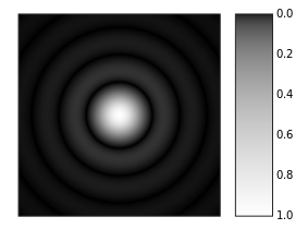
Below, I’ve inserted another image, which gives a static picture (i.e. one that is not varying in time) of the wave function of a real-life electron. To be precise: it’s the wave function for an electron on the 5d orbital of a hydrogen orbital. You can see it’s much more complicated than those easy things above. However, the idea behind is the same. We have a complex-valued function varying in space and in time. I took it from Wikipedia and so I’ll just copy the explanation here: “The solid body shows the places where the electron’s probability density is above a certain value (0.02), as calculated from the probability amplitude.” What about these colors? Well… The image uses the so-called HSL color system to represent complex numbers: each complex number is represented by a unique color, with a different hue (H), saturation (S) and lightness (L). Just google if you want to know how that works exactly.

OK. That should be clear enough. I wanted to talk about photons here. So let’s go for it. Well… Hmm… I realize I need to talk about some more ‘basics’ first. Sorry for that.

The Uncertainty Principle revisited (1)

The wave function is usually given as a function in space and time: Ψ = Ψ(x, t). However, I should also remind you that we have a similar function in the ‘momentum space’: if ψ is a psi function, then the function in the momentum space is a phi function, and we’ll write it as Φ = Φ(p, t). [As for the notation, x and p are written with capital letters and, hence, represent (three-dimensional) vectors. Likewise, we use a capital letter for psi and phi so we don’t confuse it with, for example, the lower-case φ (phi) representing the phase of a wave function.]

The position-space and momentum-space wave functions Ψ and Φ are related through the Uncertainty Principle. To be precise: they are Fourier transforms of each other. Huh? Don’t be put off by that statement. In fact, I shouldn’t have mentioned it, but then it’s how one can actually prove or derive the Uncertainty Principle from… Well… From ‘first principles’, let’s say, instead of just jotting it down as some God-given rule. Indeed, as Feynman puts: “The Uncertainty Principle should be seen in its historical context. If you get rid of all of the old-fashioned ideas and instead use the ideas that I’m explaining in these lectures—adding arrows for all the ways an event can happen—there is no need for an uncertainty principle!” However, I must assume you’re, just like me, not quite used to the new ideas as yet, and so let me just jot down the Uncertainty Principle once again, as some God-given rule indeed :-):

σ_x·σ_p≥ ħ/2

This is the so-called Kennard formulation of the Principle: it measures the uncertainty about the exact position (x) as well as the momentum (p), in terms of the standard deviation (so that’s the σ (sigma) symbol) around the mean. To be precise, the assumption is that we cannot know the real x and p: we can only find some probability distribution for x and p, which is usually some nice “bell curve” in the textbooks. While the Kennard formulation is the most precise (and exact) formulation of the Uncertainty Principle (or uncertainty relation, I should say), you’ll often find ‘other’ formulations. These ‘other’ formulates usually write Δx and Δp instead of σ_xand σ_p, with the Δ symbol indicating some ‘spread’ or a similar concept—surely do not think of Δ as a differential or so! [Sorry for assuming you don’t know this (I know you do!) but I just want to make sure here!] Also, these ‘other’ formulations will usually (a) not mention the 1/2 factor, (b) substitute ħ for h (ħ = h/2π, as you know, so ħ is preferred when we’re talking things like angular frequency or other stuff involving the unit circle), or (c) put an equality (=) sign in, instead of an inequality sign (≥). Niels Bohr’s early formulation of the Uncertainty Principle actually does all of that:

ΔxΔp = h

So… Well… That’s a bit sloppy, isn’t it? Maybe. In Feynman’s Lectures, you’ll find an oft-quoted ‘application’ of the Uncertainty Principle leading to a pretty accurate calculation of the typical size of an atom (the so-called Bohr radius), which Feynman starts with an equally sloppy statement of the Uncertainty Principle, so he notes: “We needn’t trust our answer to within factors like 2, π etcetera.” Frankly, I used to think that’s ugly and, hence, doubt the ‘seriousness’ of such kind of calculations. Now I know it doesn’t really matter indeed, as the essence of the relationship is clearly not a 2, π or 2π factor. The essence is the uncertainty itself: it’s very tiny (and multiplying it with 2, π or 2π doesn’t make it much bigger) but so it’s there.

In this regard, I need to remind you of how tiny that physical constant ħ actually is: about 6.58×10⁻¹⁶eV·s. So that’s a zero followed by a decimal point and fifteen zeroes: only then we get the first significant digits (65812…). And if 10⁻¹⁶doesn’t look tiny enough for you, then just think about how tiny the electronvolt unit is: it’s the amount of (potential) energy gained (or lost) by an electron as it moves across a potential difference of one volt (which, believe me, is nothing much really): if we’d express ħ in Joule, then we’d have to add nineteen more zeroes, because 1 eV = 1.6×10⁻¹⁹ J. As for such phenomenally small numbers, I’ll just repeat what I’ve said many times before: we just cannot imagine such small number. Indeed, our mind can sort of intuitively deal with addition (and, hence, subtraction), and with multiplication and division (but to some extent only), but our mind is not made to understand non-linear stuff, such as exponentials indeed. If you don’t believe me, think of the Richter scale: can you explain the difference between a 4.0 and a 5.0 earthquake? […] If the answer to that question took you more than a second… Well… I am right. 🙂 [The Richter scale is based on the base-10 exponential function: a 5.0 earthquake has a shaking amplitude that is 10 times that of an earthquake that registered 4.0, and because energy is proportional to the square of the amplitude, that corresponds to an energy release that is 31.6 times that of the lesser earthquake.]

A digression on units

Having said what I said above, I am well aware of the fact that saying that we cannot imagine this or that is what most people say. I am also aware of the fact that they usually say that to avoid having to explain something. So let me try to do something more worthwhile here.

1. First, I should note that ħ is so small because the second, as a unit of time, is so incredibly large. All is relative, of course. 🙂 For sure, we should express time in a more natural unit at the atomic or sub-atomic scale, like the time that’s needed for light to travel one meter. Let’s do it. Let’s express time in a unit that I shall call a ‘meter‘. Of course, it’s not an actual meter (because it doesn’t measure any distance), but so I don’t want to invent a new word and surely not any new symbol here. Hence, I’ll just put apostrophes before and after: so I’ll write ‘meter’ or ‘m’. When adopting the ‘meter’ as a unit of time, we get a value for ‘ħ‘ that is equal to (6.6×10⁻¹⁶eV·s)(1/3×10⁸ ‘meter’/second) = 2.2×10⁻⁸eV·’m’. Now, 2.2×10⁻⁸is a number that is still too tiny to imagine. But then our ‘meter’ is still a rather huge unit at the atomic scale: we should take the ‘millimicron’, aka the ‘nanometer’ (1 nm = 1×10⁻⁹ m), or – even better because more appropriate – the ‘angstrom‘: 1 Å = 0.1 nm = 1×10⁻¹⁰ m. Indeed, the smallest atom (hydrogen) has a radius of 0.25 Å, while larger atoms will have a radius of about 1 or more Å. Now that should work, isn’t it? You’re right, we get a value for ‘ħ‘ equal to (6.6×10⁻¹⁶eV·s)(1/3×10⁸ ‘m’/s)(1×10¹⁰ ‘Å’/m) = 220eV·’Å’, or 22 220eV·’nm’. So… What? Well… If anything, it shows ħ is not a small unit at the atomic or sub-atomic level! Hence, we actually can start imagining how things work at the atomic level when using more adequate units.

[Now, just to test your knowledge, let me ask you: what’s the wavelength of visible light in angstrom? […] Well? […] Let me tell you: 400 to 700 nm is 4000 to 7000 Å. In other words, the wavelength of visible light is quite sizable as compared to the size of atoms or electron orbits!]

2. Secondly, let’s do a quick dimension analysis of that ΔxΔp = h relation and/or its more accurate expression σ_x·σ_p≥ ħ/2.

A position (and its uncertainty or standard deviation) is expressed in distance units, while momentum… Euh… Well… What? […] Momentum is mass times velocity, so it’s kg·m/s. Hence, the dimension of the product on the left-hand side of the inequality is m·kg·m/s = kg·m²/s. So what about this eV·s dimension on the right-hand side? Well… The electronvolt is a unit of energy, and so we can convert it to joules. Now, a joule is a newton-meter (N·m), which is the unit for both energy and work: it’s the work done when applying a force of one newton over a distance of one meter. So we now have N·m·s for ħ, which is nice, because Planck’s constant (h or ħ—whatever: the choice for one of the two depends on the variables we’re looking at) is the quantum for action indeed. It’s a Wirkung as they say in German, so its dimension combines both energy as well as time.

To put it simply, it’s a bit like power, which is what we men are interested in when looking at a car or motorbike engine. 🙂 Power is the energy spent or delivered per second, so its dimension is J/s, not J·s. However, your mind can see the similarity in thinking here. Energy is a nice concept, be it potential (think of a water bucket above your head) or kinetic (think of a punch in a bar fight), but it makes more sense to us when adding the dimension of time (emptying a bucket of water over your head is different than walking in the rain, and the impact of a punch depends on the power with which it is being delivered). In fact, the best way to understand the dimension of Planck’s constant is probably to also write the joule in ‘base units’. Again, one joule is the amount of energy we need to move an object over a distance of one meter against a force of one newton. So one J·s is one N·m·s is (1) a force of one newton acting over a distance of (2) one meter over a time period equal to (3) one second.

I hope that gives you a better idea of what ‘action’ really is in physics. […] In any case, we haven’t answered the question. How do we relate the two sides? Simple: a newton is an oft-used SI unit, but it’s not a SI base unit, and so we should deconstruct it even more (i.e. write it in SI base units). If we do that, we get 1 N = 1 kg·m/s²: one newton is the force needed to give a mass of 1 kg an acceleration of 1 m/s per second. So just substitute and you’ll see the dimension on the right-hand side is kg·(m/s²)·m·s = kg·m²/s, so it comes out alright.

Why this digression on units? Not sure. Perhaps just to remind you also that the Uncertainty Principle can also be expressed in terms of energy and time:

ΔE·Δt = h

Here there’s no confusion in regard to the units on both sides: we don’t need to convert to SI base units to see that they’re the same: [ΔE][Δt] = J·s.

The Uncertainty Principle revisited (2)

The ΔE·Δt = h expression is not so often used as an expression of the Uncertainty Principle. I am not sure why, and I don’t think it’s a good thing. Energy and time are also complementary variables in quantum mechanics, so it’s just like position and momentum indeed. In fact, I like the energy-time expression somewhat more than the position-momentum expression because it does not create any confusion in regard to the units on both sides: it’s just joules (or electronvolts) and seconds on both sides of the equation. So what?

Frankly, I don’t want to digress too much here (this post is going to become awfully long) but, personally, I found it hard, for quite a while, to relate the two expressions of the very same uncertainty ‘principle’ and, hence, let me show you how the two express the same thing really, especially because you may or may not know that there are even more pairs of complementary variables in quantum mechanics. So, I don’t know if the following will help you a lot, but it helped me to note that:

The energy and momentum of a particle are intimately related through the (relativistic) energy-momentum relationship. Now, that formula, E² = p²c² – m₀²c⁴, which links energy, momentum and intrinsic mass (aka rest mass), looks quite monstrous at first. Hence, you may prefer a simpler form: pc = Ev/c. It’s the same really as both are based on the relativistic mass-energy equivalence: E = mc² or, the way I prefer to write it: m = E/c². [Both expressions are the same, obviously, but we can ‘read’ them differently: m = E/c² expresses the idea that energy has a equivalent mass, defined as inertia, and so it makes energy the primordial concept, rather than mass.] Of course, you should note that m is the total mass of the object here, including both (a) its rest mass as well as (b) the equivalent mass it gets from moving at the speed v. So m, not m₀, is the concept of mass used to define p, and note how easy it is to demonstrate the equivalence of both formulas: pc = Ev/c ⇔ mvc = Ev/c ⇔ E = mc². In any case, the bottom line is: don’t think of the energy and momentum of a particle as two separate things; they are two aspects of the same ‘reality’, involving mass (a measure of inertia, as you know) and velocity (as measured in a particular (so-called inertial) reference frame).
Time and space are intimately related through the universal constant c, i.e. the speed of light, as evidenced by the fact that we will often want to express distance not in meter but in light-seconds (i.e. the distance that light travels (in a vacuum) in one second) or, vice versa, express time in meter (i.e. the time that light needs to travel a distance of one meter).

These relationships are interconnected, and the following diagram shows how.

The easiest way to remember it all is to apply the Uncertainty Principle, in both its ΔE·Δt = h as well as its Δp·Δx = h expressions, to a photon. A photon has no rest mass and its velocity v is, obviously, c. So the energy-momentum relationship is a very simple one: p = E/c. We then get both expressions of the Uncertainty Principle by simply substituting E for p, or vice versa, and remember that time and position (or distance) are related in exactly the same way: the constant of proportionality is the very same. It’s c. So we can write: Δx = Δt·c and Δt = Δx/c. If you’re confused, think about it in very practical terms: because the speed of light is what it is, an uncertainty of a second in time amounts, roughly, to an uncertainty in position of some 300,000 km (c = 3×10⁸m/s). Conversely, an uncertainty of some 300,000 km in the position amounts to a uncertainty in time of one second. That’s what the 1-2-3 in the diagram above is all about: please check if you ‘get’ it, because that’s ‘essential’ indeed.

Back to ‘probability waves’

Matter-particles are not the same, but we do have the same relations, including that ‘energy-momentum duality’. The formulas are just somewhat more complicated because they involve mass and velocity (i.e. a velocity less than that of light). For matter-particles, we can see that energy-momentum duality not only in the relationships expressed above (notably the relativistic energy-momentum relation), but also in the (in)famous de Broglie relation, which associates some ‘frequency’ (f) to the energy (E) of a particle or, what amounts to the same, some ‘wavelength’ (λ) to its momentum (p):

λ = h/p and f = E/h

These two complementary equations give a ‘wavelength’ (λ) and/or a ‘frequency’ (f) of a de Broglie wave, or a ‘matter wave’ as it’s sometimes referred to. I am using, once again, apostrophes because the de Broglie wavelength and frequency are a different concept—different than the wavelength or frequency of light, or of any other ‘real’ wave (like water or sound waves, for example). To illustrate the differences, let’s start with a very simple question: what’s the velocity of a de Broglie wave? Well… […] So? You thought you knew, didn’t you?

Let me answer the question:

The mathematically (and physically) correct answer involves distinguishing the group and phase velocity of a wave.
The ‘easy’ answer is: the de Broglie wave of a particle moves with the particle and, hence, its velocity is, obviously, the speed of the particle which, for electrons, is usually non-relativistic (i.e. rather slow as compared to the speed of light).

To be clear on this, the velocity of a de Broglie wave is not the speed of light. So a de Broglie wave is not like an electromagnetic wave at all. They have nothing in common really, except for the fact that we refer to both of them as ‘waves’. 🙂

The second thing to note is that, when we’re talking about the ‘frequency’ or ‘wavelength’ of ‘matter waves’ (i.e. de Broglie waves), we’re talking the frequency and wavelength of a wave with two components: it’s a complex-valued wave function, indeed, and so we get a real and imaginary part when we’re ‘feeding’ the function with some values for x and t.

Thirdly and, perhaps, most importantly, we should always remember the Uncertainty Principle when looking at the de Broglie relation. The Uncertainty Principle implies that we can actually not assign any precise wavelength (or, what amounts to the same, a precise frequency) to a de Broglie wave: if there is a spread in p (and, hence, in E), then there will be a spread in λ (and in f). In fact, I tend to think that it would be better to write the de Broglie relation as an ‘uncertainty relation’ in its own right:

Δλ = Δ(h/p) = hΔp and Δf = ΔE/h = hΔE

Besides from underscoring the fact that we have other ‘pairs’ of complementary variables, this ‘version’ of the de Broglie equation would also remind us continually of the fact that a ‘regular’ wave with an exact frequency and/or an exact wavelength (so a Δλ and/or a Δf equal to zero) would not give us any information about the momentum and/or the energy. Indeed, as Δλ and/or Δf go to zero (Δλ → 0 and/or Δf → 0 ), then Δp and ΔE must go to infinity (Δp → ∞ and ΔE → ∞. That’s just the math involved in such expressions. 🙂

Jokes aside, I’ll admit I used to have a lot of trouble understanding this, so I’ll just quote the expert teacher (Feynman) on this to make sure you don’t get me wrong here:

“The amplitude to find a particle at a place can, in some circumstances, vary in space and time, let us say in one dimension, in this manner: Ψ = Ae^i(ωt−kx), where ω is the frequency, which is related to the classical idea of the energy through E = ħω, and k is the wave number, which is related to the momentum through p = ħk. [These are equivalent formulations of the de Broglie relations using the angular frequency and the wave number instead of wavelength and frequency.] We would say the particle had a definite momentum p if the wave number were exactly k, that is, a perfect wave which goes on with the same amplitude everywhere. The Ψ = Ae^i(ωt−kx)equation [then] gives the [complex-valued probability] amplitude, and if we take the absolute square, we get the relative probability for finding the particle as a function of position and time. This is a constant, which means that the probability to find a [this] particle is the same anywhere.” (Feynman’s Lectures, I-48-5)

You may say or think: What’s the problem here really? Well… If the probability to find a particle is the same anywhere, then the particle can be anywhere and, for all practical purposes, that amounts to saying it’s nowhere really. Hence, that wave function doesn’t serve the purpose. In short, that nice Ψ = Ae^i(ωt−kx)function is completely useless in terms of representing an electron, or any other actual particle moving through space. So what to do?

The Wikipedia article on the Uncertainty Principle has this wonderful animation that shows how we can superimpose several waves, one on top of each other, to form a wave packet. Let me copy it below:

So that’s what the wave we want indeed: a wave packet that travels through space but which is, at the same time, limited in space. Of course, you should note, once again, that it shows only one part of the complex-valued probability amplitude: just visualize the other part (imaginary if the wave above would happen to represent the real part, and vice versa if the wave would happen to represent the imaginary part of the probability amplitude). The animation basically illustrates a mathematical operation. To be precise, it involves a Fourier analysis or decomposition: it separates a wave packet into a finite or (potentially) infinite number of component waves. Indeed, note how, in the illustration above, the frequency of the component waves gradually increases (or, what amounts to the same, how the wavelength gets smaller and smaller) and how, with every wave we ‘add’ to the packet, it becomes increasingly localized. Now, you can easily see that the ‘uncertainty’ or ‘spread’ in the wavelength here (which we’ll denote by Δλ) is, quite simply, the difference between the wavelength of the ‘one-cycle wave’, which is equal to the space the whole wave packet occupies (which we’ll denote by Δx), and the wavelength of the ‘highest-frequency wave’. For all practical purposes, they are about the same, so we can write: Δx ≈ Δλ. Using Bohr’s formulation of the Uncertainty Principle, we can see the expression I used above (Δλ = hΔp) makes sense: Δx = Δλ = h/Δp, so ΔλΔp = h.

[Just to be 100% clear on terminology: a Fourier decomposition is not the same as that Fourier transform I mentioned when talking about the relation between position and momentum in the Kennard formulation of the Uncertainty Principle, although these two mathematical concepts obviously have a few things in common.]

The wave train revisited

All what I’ve said above, is the ‘correct’ interpretation of the Uncertainty Principle and the de Broglie equation. To be frank, it took me quite a while to ‘get’ that—and, as you can see, it also took me quite a while to get ‘here’, of course. 🙂

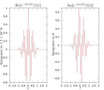
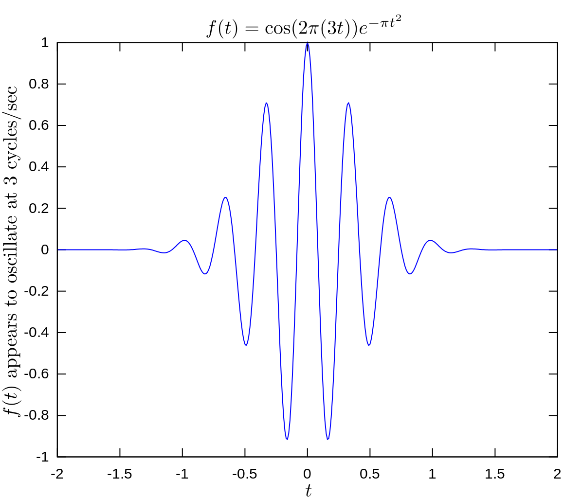
In fact, I was confused, for quite a few years actually, because I never quite understood whey there had to be a spread in the wavelength of a wave train. Indeed, we can all easily imagine a localized wave train with a fixed frequency and a fixed wavelength, like the one below, which I’ll re-use later. I’ve made this wave train myself: it’s a standard sine and cosine function multiplied with an ‘envelope’ function generating the envelope. As you can see, it’s a complex-valued thing indeed: the blue curve is the real part, and the imaginary part is the red curve.

You can easily make a graph like this yourself. [Just use of one of those online graph tools.] This thing is localized in space and, as mentioned above, it has a fixed frequency and wavelength. So all those enigmatic statements you’ll find in serious or less serious books (i.e. textbooks or popular accounts) on quantum mechanics saying that “we cannot define a unique wavelength for a short wave train” and/or saying that “there is an indefiniteness in the wave number that is related to the finite length of the train, and thus there is an indefiniteness in the momentum” (I am quoting Feynman here, so not one of the lesser gods) are – with all due respect for these authors, especially Feynman – just wrong. I’ve made another ‘short wave train’ below, but this time it depicts the real part of a (possible) wave function only.

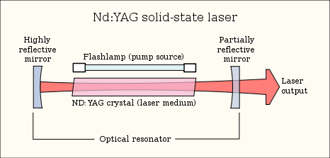
Hmm… Now that one has a weird shape, you’ll say. It doesn’t look like a ‘matter wave’! Well… You’re right. Perhaps. [I’ll challenge you in a moment.] The shape of the function above is consistent, though, with the view of a photon as a transient electromagnetic oscillation. Let me come straight to the point by stating the basics: the view of a photon in physics is that photons are emitted by atomic oscillators. As an electron jumps from one energy level to the other, it seems to oscillate back and forth until it’s in equilibrium again, thereby emitting an electromagnetic wave train that looks like a transient.

Huh? What’s a transient? It’s an oscillation like the one above: its amplitude and, hence, its energy, gets smaller and smaller as time goes by. To be precise, its energy level has the same shape as the envelope curve below: E = E₀e^–t/τ. In this expression, we have τ as the so-called decay time, and one can show it’s the inverse of the so-called decay rate: τ = 1/γ with γE = –dE/dt. In case you wonder, check it out on Wikipedia: it’s one of the many applications of the natural exponential function: we’re talking a so-called exponential decay here indeed, involves a quantity (in this case, the amplitude and/or the energy) decreasing at a rate that is proportional to its current value, with the coefficient of proportionality being γ. So we write that as γE = –dE/dt in mathematical notation. 🙂

I need to move on. All of what I wrote above was ‘plain physics’, but so what I really want to explore in this post is a crazy hypothesis. Could these wave trains above – I mean the wave trains with the fixed frequency and wavelength – possible represent a de Broglie wave for a photon?

You’ll say: of course not! But, let’s be honest, you’d have some trouble explaining why. The best answer you could probably come up with is: because no physics textbook says something like that. You’re right. It’s a crazy hypothesis because, when you ask a physicist (believe it or not, but I actually went through the trouble of asking two nuclear scientists), they’ll tell you that photons are not to be associated with de Broglie waves. [You’ll say: why didn’t you try looking for an answer on the Internet? I actually did but – unlike what I am used to – I got very confusing answers on this one, so I gave up trying to find some definite answer on this question on the Internet.]

However, these negative answers don’t discourage me from trying to do some more freewheeling. Before discussing whether or not the idea of a de Broglie wave for a photon makes sense, let’s think about mathematical constraints. I googled a bit but I only see one actually: the amplitudes of a de Broglie wave are subject to a normalization condition. Indeed, when everything is said and done, all probabilities must take a value between 0 and 1, and they must also all add up to exactly 1. So that’s a so-called normalization condition that obviously imposes some constraints on the (complex-valued) probability amplitudes of our wave function.

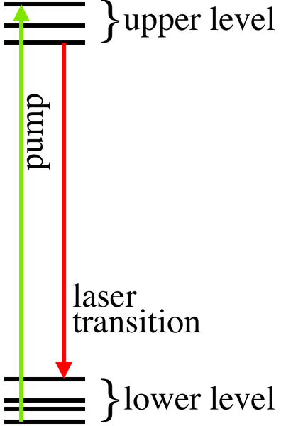
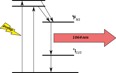
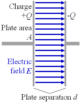
But let’s get back to the photon. Let me remind you of what happens when a photon is being emitted by inserting the two diagrams below, which gives the energy levels of the atomic orbitals of electrons.

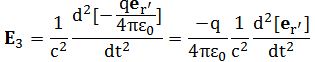
So an electron absorbs or emits a photon when it goes from one energy level to the other, so it absorbs or emits radiation. And, of course, you will also remember that the frequency of the absorbed or emitted light is related to those energy levels. More specifically, the frequency of the light emitted in a transition from, let’s say, energy level E₃to E₁will be written as ν₃₁= (E₃– E₁)/h. This frequency will be one of the so-called characteristic frequencies of the atom and will define a specific so-called spectral emission line.

Now, from a mathematical point of view, there’s no difference between that ν₃₁= (E₃– E₁)/h equation and the de Broglie equation, f = E/h, which assigns a de Broglie wave to a particle. But, of course, from all that I wrote above, it’s obvious that, while these two formulas are the same from a math point of view, they represent very different things. Again, let me repeat what I said above: a de Broglie wave is a matter-wave and, as such, it has nothing to do with an electromagnetic wave.

Let me be even more explicit. A de Broglie wave is not a ‘real’ wave, in a sense (but, of course, that’s a very unscientific statement to make); it’s a psi function, so it represents these weird mathematical quantities–complex probability amplitudes–which allow us to calculate the probability of finding the particle at position x or, if it’s a wave function for the momentum-space, to find a value p for its momentum. In contrast, a photon that’s emitted or absorbed represents a ‘real’ disturbance of the electromagnetic field propagating through space. Hence, that frequency ν is something very different than f, which is why we use another symbol for it (ν is the Greek letter nu, not to be confused with the v symbol we use for velocity). [Of course, you may wonder how ‘real’ or ‘unreal’ an electromagnetic field is but, in the context of this discussion, let me assure you we should look at it as something that’s very real.]

That being said, we also know light is emitted in discrete energy packets: in fact, that’s how photons were defined originally, first by Planck and then by Einstein. Now, when an electron falls from one energy level in an atom to another (lower) energy level, it emits one – and only one – photon with that particular wavelength and energy. The question then is: how should we picture that photon? Does it also have some more or less defined position in space, and some momentum? The answer is definitely yes, on both accounts:

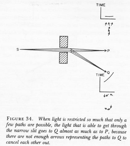
Subject to the constraints of the Uncertainty Principle, we know, more or less indeed, when a photon leaves a source and when it hits some detector. [And, yes, due to the ‘Uncertainty Principle’ or, as Feynman puts it, the rules for adding arrows, it may not travel in a straight line and/or at the speed of light—but that’s a discussion that, believe it or not, is not directly relevant here. If you want to know more about it, check one or more of my posts on it.]
We also know light has a very definite momentum, which I’ve calculated elsewhere and so I’ll just note the result: p = E/c. It’s a ‘pushing momentum’ referred to as radiation pressure, and its in the direction of travel indeed.

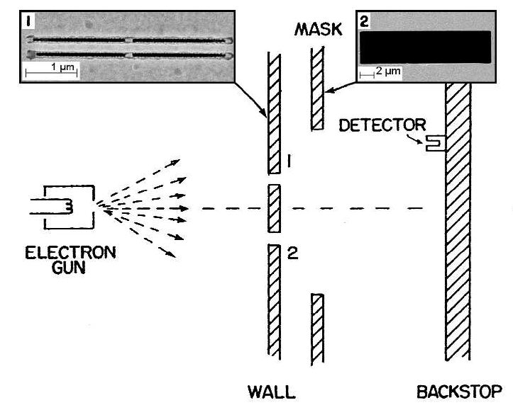
In short, it does makes sense, in my humble opinion that is, to associate some wave function with the photon, and then I mean a de Broglie wave. Just think about it yourself. You’re right to say that a de Broglie wave is a ‘matter wave’, and photons aren’t matter but, having said that, photons do behave like like electrons, don’t they? There’s diffraction (when you send a photon through one slit) and interference (when photons go through two slits, altogether or – amazingly – one by one), so it’s the same weirdness as electrons indeed, and so why wouldn’t we associate some kind of wave function with them?

You can react in one of three ways here. The first reaction is: “Well… I don’t know. You tell me.” Well… That’s what I am trying to do here. 🙂

The second reaction may be somewhat more to the point. For example, those who’ve read Feynman’s Strange Theory of Light and Matter, could say: “Of course, why not? That’s what we do when we associate a photon going from point A to B with an amplitude P(A to B), isn’t it?”

Well… No. I am talking about something else here. Not some amplitude associated with a path in spacetime, but a wave function giving an approximate position of the photon.

The third reaction may be the same as the reaction of those two nuclear scientists I asked: “No. It doesn’t make sense. We do not associate photons with a de Broglie wave.” But so they didn’t tell me why because… Well… They didn’t have the time to entertain a guy like me and so I didn’t dare to push the question and continued to explore it more in detail myself.

So I’ve done that, and I thought of one reason why the question, perhaps, may not make all that much sense: a photon travels at the speed of light; therefore, it has no length. Hence, doing what I am doing below, and that’s to associate the electromagnetic transient with a de Broglie wave might not make sense.

Maybe. I’ll let you judge. Before developing the point, I’ll raise two objections to the ‘objection’ raised above (i.e. the statement that a photon has no length). First, if we’re looking at the photon as some particle, it will obviously have no length. However, an electromagnetic transient is just what it is: an electromagnetic transient. I’ve see nothing that makes me think its length should be zero. In fact, if that would be the case, the concept of an electromagnetic wave itself would not make sense, as its ‘length’ would always be zero. Second, even if – somehow – the length of the electromagnetic transient would be reduced to zero because of its speed, we can still imagine that we’re looking at the emission of an electromagnetic pulse (i.e. a photon) using the reference frame of the photon, so that we’re traveling at speed c,’ riding’ with the photon, so to say, as it’s being emitted. Then we would ‘see’ the electromagnetic transient as it’s being radiated into space, wouldn’t we?

Perhaps. I actually don’t know. That’s why I wrote this post and hope someone will react to it. I really don’t know, so I thought it would be nice to just freewheel a bit on this question. So be warned: nothing of what I write below has been researched really, so critical comments and corrections from actual specialists are more than welcome.

The shape of a photon wave

As mentioned above, the answer in regard to the definition of a photon’s position and momentum is, obviously, unambiguous. Perhaps we have to stretch whatever we understand of Einstein’s (special) relativity theory, but we should be able to draw some conclusions, I feel.

Let me say one thing more about the momentum here. As said, I’ll refer you to one of my posts for the detail but, all you should know here is that the momentum of light is related to the magnetic field vector, which we usually never mention when discussing light because it’s so tiny as compared to the electric field vector in our inertial frame of reference. Indeed, the magnitude of the magnetic field vector is equal to the magnitude of the electric field vector divided by c = 3×10⁸, so we write B = E/c. Now, the E here stands for the electric field, so let me use W to refer to the energy instead of E. Using the B = E/c equation and a fairly straightforward calculation of the work that can be done by the associated force on a charge that’s being put into this field, we get that famous equation which we mentioned above already: the momentum of a photon is its total energy divided by c, so we write p = W/c. You’ll say: so what? Well… Nothing. I just wanted to note we get the same p = W/c equation indeed, but from a very different angle of analysis here. We didn’t use the energy-momentum relation here at all! In any case, the point to note is that the momentum of a photon is only a tiny fraction of its energy (p = W/c), and that the associated magnetic field vector is also just a tiny fraction of the electric field vector (B = E/c).

But so it’s there and, in fact, when adopting a moving reference frame, the mix of E and B (i.e. the electric and magnetic field) becomes an entirely different one. One of the ‘gems’ in Feynman’s Lectures is the exposé on the relativity of electric and magnetic fields indeed, in which he analyzes the electric and magnetic field caused by a current, and in which he shows that, if we switch our inertial reference frame for that of the moving electrons in the wire, the ‘magnetic’ field disappears, and the whole electromagnetic effect becomes ‘electric’ indeed.

I am just noting this because I know I should do a similar analysis for the E and B ‘mixture’ involved in the electromagnetic transient that’s being emitted by our atomic oscillator. However, I’ll admit I am not quite comfortably enough with the physics nor the math involved to do that, so… Well… Please do bear this in mind as I will be jotting down some quite speculative thoughts in what follows.

So… A photon is, in essence, a electromagnetic disturbance and so, when trying to picture a photon, we can think of some oscillating electric field vector traveling through–and also limited in–space. [Note that I am leaving the magnetic field vector out of the analysis from the start, which is not ‘nice’ but, in light of that B = E/c relationship, I’ll assume it’s acceptable.] In short, in the classical world – and in the classical world only of course – a photon must be some electromagnetic wave train, like the one below–perhaps.

But why would it have that shape? I only suggested it because it has the same shape as Feynman’s representation of a particle (see below) as a ‘probability wave’ traveling through–and limited in–space.

So, what about it? Let me first remind you once again (I just can’t stress this point enough it seems) that Feynman’s representation – and most are based on his, it seems – is misleading because it suggests that ψ(x) is some real number. It’s not. In the image above, the vertical axis should not represent some real number (and it surely should not represent a probability, i.e. some real positive number between 0 and 1) but a probability amplitude, i.e. a complex number in which both the real and imaginary part are important. Just to be fully complete (in case you forgot), such complex-valued wave function ψ(x) will give you all the probabilities you need when you take its (absolute) square, but so… Well… We’re really talking a different animal here, and the image above gives you only one part of the complex-valued wave function (either the real or the imaginary part), while it should give you both. That’s why I find my graph below much better. 🙂 It’s the same really, but so it shows both the real as well as the complex part of a wave function.

But let me go back to the first illustration: the vertical axis of the first illustration is not ψ but E – the electric field vector. So there’s no imaginary part here: just a real number, representing the strength–or magnitude I should say– of the electric field E as a function of the space coordinate x. [Can magnitudes be negative? The honest answer is: no, they can’t. But just think of it as representing the field vector pointing in the other way .]

Regardless of the shortcomings of this graph, including the fact we only have some real-valued oscillation here, would it work as a ‘suggestion’ of how a real-life photon could look like?

Of course, you could try to not answer that question by mumbling something like: “Well… It surely doesn’t represent anything coming near to a photon in quantum mechanics.” But… Well… That’s not my question here: I am asking you to be creative and ‘think outside of the box’, so to say. 🙂

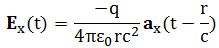
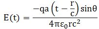
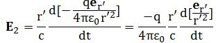
So you should say ‘No!’ because of some other reason. What reason? Well… If a photon is an electromagnetic transient – in other words, if we adopt a purely classical point of view – it’s going to be a transient wave indeed, and so then it should walk, talk and even look like a transient. 🙂 Let me quickly jot down the formula for the (vertical) component of E as a function of the acceleration of some charge q:

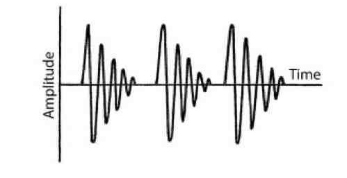
The charge q (i.e. the source of the radiation) is, of course, our electron that’s emitting the photon as it jumps from a higher to a lower energy level (or, vice versa, absorbing it). This formula basically states that the magnitude of the electric field (E) is proportional to the acceleration (a) of the charge (with t–r/c the retarded argument). Hence, the suggested shape of E as a function of x as shown above would imply that the acceleration of the electron is (a) initially quite small, (b) then becomes larger and larger to reach some maximum, and then (c) becomes smaller and smaller again to then die down completely. In short, it does match the definition of a transient wave sensu stricto (Wikipedia defines a transient as “a short-lived burst of energy in a system caused by a sudden change of state”) but it’s not likely to represent any real transient. So, we can’t exclude it, but a real transient is much more likely to look like something what’s depicted below: no gradual increase in amplitude but big swings initially which then dampen to zero. In other words, if our photon is a transient electromagnetic disturbance caused by a ‘sudden burst of energy’ (which is what that electron jump is, I would think), then its representation will, much more likely, resemble a damped wave, like the one below, rather than Feynman’s picture of a moving matter-particle.

In fact, we’d have to flip the image, both vertically and horizontally, because the acceleration of the source and the field are related as shown below. The vertical flip is because of the minus sign in the formula for E(t). The horizontal flip is because of the minus sign in the (t – r/c) term, the retarded argument: if we add a little time (Δt), we get the same value for a(t−r/c) as we would have if we had subtracted a little distance: Δr=−cΔt. So that’s why E as a function of r (or of x), i.e. as a function in space, is a ‘reversed’ plot of the acceleration as a function of time.

So we’d have something like below.

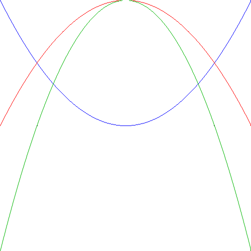
What does this resemble? It’s not a vibrating string (although I do start to understand the attractiveness of string theory now: vibrating strings are great as energy storage systems, so the idea of a photon being some kind of vibrating string sounds great, doesn’t it?). It’s not resembling a bullwhip effect either, because the oscillation of a whip is confined by a different envelope (see below). And, no, it’s also definitely not a trumpet. 🙂

It’s just what it is: an electromagnetic transient traveling through space. Would this be realistic as a ‘picture’ of a photon? Frankly, I don’t know. I’ve looked at a lot of stuff but didn’t find anything on this really. The easy answer, of course, is quite straightforward: we’re not interested in the shape of a photon because we know it is not an electromagnetic wave. It’s a ‘wavicle’, just like an electron.

[…] Sure. I know that too. Feynman told me. 🙂 But then why wouldn’t we associate some wave function with it? Please tell me, because I really can’t find much of an answer to that question in the literature, and so that’s why I am freewheeling here. So just go along with me for a while, and come up with another suggestion. As I said above, your bet is as good as mine. All that I know is that there’s one thing we need to explain when considering the various possibilities: a photon has a very well-defined frequency (which defines its color in the visible light spectrum) and so our wave train should – in my humble opinion – also have that frequency. At least for ‘quite a while’—and then I mean ‘most of the time’, or ‘on average’ at least. Otherwise the concept of a frequency – or a wavelength – wouldn’t make much sense. Indeed, if the photon has no defined wavelength or frequency, then we could not perceive it as some color (as you may or may not know, the sense of ‘color’ is produced by our eye and brain, but so it’s definitely associated with the frequency of the light). A photon should have a color (in phyics, that means a frequency) because, when everything is said and done, that’s what the Planck relation is all about.

What would be your alternative? I mean… Doesn’t it make sense to think that, when jumping from one energy level to the other, the electron would initially sort of overshoot its new equilibrium position, to then overshoot it again on the other side, and so on and so on, but with an amplitude that becomes smaller and smaller as the oscillation dies out? In short, if we look at radiation as being caused by atomic oscillators, why would we not go all the way and think of them as oscillators subject to some damping force? Just think about it. 🙂

The size of a photon wave

Let’s forget about the shape for a while and think about size. We’ve got an electromagnetic train here. So how long would it be? Well… Feynman calculated the Q of these atomic oscillators: it’s of the order of 10⁸(see his Lectures, I-33-3: it’s a wonderfully simple exercise, and one that really shows his greatness as a physics teacher) and, hence, this wave train will last about 10^–8seconds (that’s the time it takes for the radiation to die out by a factor 1/e). To give a somewhat more precise example, for sodium light, which has a frequency of 500 THz (500×10¹²oscillations per second) and a wavelength of 600 nm (600×10^–9meter), the radiation will lasts about 3.2×10^–8seconds. [In fact, that’s the time it takes for the radiation’s energy to die out by a factor 1/e, so(i.e. the so-called decay time τ), so the wavetrain will actually last longer, but so the amplitude becomes quite small after that time.]

So that’s a very short time, but still, taking into account the rather spectacular frequency (500 THz) of sodium light, that still makes for some 16 million oscillations and, taking into the account the rather spectacular speed of light (3×10⁸m/s), that makes for a wave train with a length of, roughly, 9.6 meter. Huh? 9.6 meter!?

You’re right. That’s an incredible distance: it’s like infinity on an atomic scale!

So… Well… What to say? Such length surely cannot match the picture of a photon as a fundamental particle which cannot be broken up, can it? So it surely cannot be right because, if this would be the case, then there surely must be some way to break this thing up and, hence, it cannot be ‘elementary’, can it?

Well… Maybe. But think it through. First note that we will not see the photon as a 10-meter long string because it travels at the speed of light indeed and so the length contraction effect ensure its length, as measured in our reference frame (and from whatever ‘real-life’ reference frame actually, because the speed of light will always be c, regardless of the speeds we mortals could ever reach (including speeds close to c), is zero.

So, yes, I surely must be joking here but, as far as jokes go, I can’t help thinking this one is fairly robust from a scientific point of view. Again, please do double-check and correct me, but all what I’ve written so far is not all that speculative. It corresponds to all what I’ve read about it: only one photon is produced per electron in any de-excitation, and its energy is determined by the number of energy levels it drops, as illustrated (for a simple hydrogen atom) below. For those who continue to be skeptical about my sanity here, I’ll quote Feynman once again:

“What happens in a light source is that first one atom radiates, then another atom radiates, and so forth, and we have just seen that atoms radiate a train of waves only for about 10^–8 sec; after 10^–8 sec, some atom has probably taken over, then another atom takes over, and so on. So the phases can really only stay the same for about 10^–8 sec. Therefore, if we average for very much more than 10^–8 sec, we do not see an interference from two different sources, because they cannot hold their phases steady for longer than 10^–8 sec. With photocells, very high-speed detection is possible, and one can show that there is an interference which varies with time, up and down, in about 10^–8 sec.” (Feynman’s Lectures, I-34-4)

So… Well… Now it’s up to you. I am going along here with the assumption that a photon in the visible light spectrum, from a classical world perspective, should indeed be something that’s several meters long and packs a few million oscillations. So, while we usually measure stuff in seconds, or hours, or years, and, hence, while we would that think 10^–8seconds is short, a photon would actually be a very stretched-out transient that occupies quite a lot of space. I should also add that, in light of that number of ten meter, the dampening seems to happen rather slowly!

[…]

I can see you shaking your head now, for various reasons.

First because this type of analysis is not appropriate. […] You think so? Well… I don’t know. Perhaps you’re right. Perhaps we shouldn’t try to think of a photon as being something different than a discrete packet of energy. But then we also know it is an electromagnetic wave. So why wouldn’t we go all the way?

Second, I guess you may find the math involved in this post not to your liking, even if it’s quite simple and I am not doing anything spectacular here. […] Well… Frankly, I don’t care. Let me bulldozer on. 🙂

What about the ‘vertical’ dimension, the y and the z coordinates in space? We’ve got this long snaky thing: how thick-bodied is it?

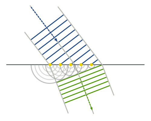
Here, we need to watch our language. While it’s fairly obvious to associate a wave with a cross-section that’s normal to its direction of propagation, it is not obvious to associate a photon with the same thing. Not at all actually: as that electric field vector E oscillates up and down (or goes round and round, as shown in the illustration below, which is an image of a circularly polarized wave), it does not actually take any space. Indeed, the electric and magnetic field vectors E and B have a direction and a magnitude in space but they’re not representing something that is actually taking up some small or larger core in space.

Hence, the vertical axis of that graph showing the wave train does not indicate some spatial position: it’s not a y-coordinate but the magnitude of an electric field vector. [Just to underline the fact that the magnitude E has nothing to do with spatial coordinates: note that its value depends on the unit we use to measure field strength (so that’s newton/coulomb, if you want to know), so it’s really got nothing to do with an actual position in space-time.]

So, what can we say about it? Nothing much, perhaps. But let me try.

Cross-sections in nuclear physics

In nuclear physics, the term ‘cross-section’ would usually refer to the so-called Thompson scattering cross-section of an electron (or any charged particle really), which can be defined rather loosely as the target area for the incident wave (i.e. the photons): it is, in fact, a surface which can be calculated from what is referred to as the classical electron radius, which is about 2.82×10^–15 m. Just to compare: you may or may not remember the so-called Bohr radius of an atom, which is about 5.29×10^–11 m, so that’s a length that’s about 20,000 times longer. To be fully complete, let me give you the exact value for the Thompson scattering cross-section of an electron: 6.62×10^–29 m²(note that this is a surface indeed, so we have m squared as a unit, not m).

Now, let me remind you – once again – that we should not associate the oscillation of the electric field vector with something actually happening in space: an electromagnetic field does not move in a medium and, hence, it’s not like a water or sound wave, which makes molecules go up and down as it propagates through its medium. To put it simply: there’s nothing that’s wriggling in space as that photon is flashing through space. However, when it does hit an electron, that electron will effectively ‘move’ (or vibrate or wriggle or whatever you can imagine) as a result of the incident electromagnetic field.

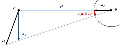
That’s what’s depicted and labeled below: there is a so-called ‘radial component’ of the electric field, and I would say: that’s our photon! [What else would it be?] The illustration below shows that this ‘radial’ component is just E for the incident beam and that, for the scattered beam, it is, in fact, determined by the electron motion caused by the incident beam through that relation described above, in which a is the normal component (i.e. normal to the direction of propagation of the outgoing beam) of the electron’s acceleration.

Now, before I proceed, let me remind you once again that the above illustration is, once again, one of those illustrations that only wants to convey an idea, and so we should not attach too much importance to it: the world at the smallest scale is best not represented by a billiard ball model. In addition, I should also note that the illustration above was taken from the Wikipedia article on elastic scattering (i.e. Thomson scattering), which is only a special case of the more general Compton scattering that actually takes place. It is, in fact, the low-energy limit. Photons with higher energy will usually be absorbed, and then there will be a re-emission, but, in the process, there will be a loss of energy in this ‘collision’ and, hence, the scattered light will have lower energy (and, hence, lower frequency and longer wavelength). But – Hey! – now that I think of it: that’s quite compatible with my idea of damping, isn’t it? 🙂 [If you think I’ve gone crazy, I am really joking here: when it’s Compton scattering, there’s no ‘lost’ energy: the electron will recoil and, hence, its momentum will increase. That’s what’s shown below (credit goes to the HyperPhysics site).]

So… Well… Perhaps we should just assume that a photon is a long wave train indeed (as mentioned above, ten meter is very long indeed: not an atomic scale at all!) but that its effective ‘radius’ should be of the same order as the classical electron radius. So what’s that order? If it’s more or less the same radius, then it would be in the order of femtometers (1 fm = 1 fermi = 1×10^–15 m). That’s good because that’s a typical length-scale in nuclear physics. For example, it would be comparable with the radius of a proton. So we look at a photon here as something very different – because it’s so incredibly long (at least as measured from its own reference frame) – but as something which does have some kind of ‘radius’ that is normal to its direction of propagation and equal or smaller than the classical electron radius. [Now that I think of it, we should probably think of it as being substantially smaller. Why? Well… An electron is obviously fairly massive as compared to a photon (if only because an electron has a rest mass and a photon hasn’t) and so… Well… When everything is said and done, it’s the electron that absorbs a photon–not the other way around!]

Now, that radius determines the area in which it may produce some effect, like hitting an electron, for example, or like being detected in a photon detector, which is just what this so-called radius of an atom or an electron is all about: the area which is susceptible of being hit by some particle (including a photon), or which is likely to emit some particle (including a photon). What is exactly, we don’t know: it’s still as spooky as an electron and, therefore, it also does not make all that much sense to talk about its exact position in space. However, if we’d talk about its position, then we should obviously also invoke the Uncertainty Principle, which will give us some upper and lower bounds for its actual position, just like it does for any other particle: the uncertainty about its position will be related to the uncertainty about its momentum, and more knowledge about the former, will implies less knowledge about the latter, and vice versa. Therefore, we can also associate some complex wave function with this photon which is – for all practical purposes – a de Broglie wave. Now how should we visualize that wave?

Well… I don’t know. I am actually not going to offer anything specific here. First, it’s all speculation. Second, I think I’ve written too much rubbish already. However, if you’re still reading, and you like this kind of unorthodox application of electromagnetics, then the following remarks may stimulate your imagination.

The first thing to note is that we should not end up with a wave function that, when squared, gives us a constant probability for each and every point in space. No. The wave function needs to be confined in space and, hence, we’re also talking a wave train here, and a very short one in this case. So… Well… What about linking its amplitude to the amplitude of the field for the photon. In other words, the probability amplitude could, perhaps, be proportional to the amplitude of E, with the proportionality factor being determined by (a) the unit in which we measure E (i.e. newton/coulomb) and (b) the normalization condition.

OK. I hear you say it now: “Ha-ha! Got you! Now you’re really talking nonsense! How can a complex number (the probability amplitude) be proportional to some real number (the field strength)?”

Well… Be creative. It’s not that difficult to imagine some linkages. First, the electric field vector has both a magnitude and a direction. Hence, there’s more to E than just its magnitude. Second, you should note that the real and imaginary part of a complex-valued wave function is a simple sine and cosine function, and so these two functions are the same really, except for a phase difference of π/2. In other words, if we have a formula for the real part of a wave function, we have a formula for its imaginary part as well. So… Your remark is to the point and then it isn’t.

OK, you’ll say, but then so how exactly would you link the E vector with the ψ(x, t) function for a photon. Well… Frankly, I am a bit exhausted now and so I’ll leave any further speculation to you. The whole idea of a de Broglie wave of a photon, with the (complex-valued) amplitude having some kind of ‘proportional’ relationship to the (magnitude of) the electric field vector makes sense to me, although we’d have to be innovative about what that ‘proportionality’ exactly is.

Let me conclude this speculative business by noting a few more things about our ‘transient’ electromagnetic wave:

1. First, it’s obvious that the usual relations between (a) energy (W), (b) frequency (f) and (c) amplitude (A) hold. If we increase the frequency of a wave, we’ll have a proportional increase in energy (twice the frequency is twice the energy), with the factor of proportionality being given by the Planck-Einstein relation: W = hf. But if we’re talking amplitudes (for which we do not have a formula, which is why we’re engaging in those assumptions on the shape of the transient wave), we should not forget that the energy of a wave is proportional to the square of its amplitude: W ∼ A². Hence, a linear increase of the amplitudes results in an exponential (quadratic) increase in energy (e.g. if you double all amplitudes, you’ll pack four times more energy in that wave).

2. Both factors come into play when an electron emits a photon. Indeed, if the difference between the two energy levels is larger, then the photon will not only have a higher frequency (i.e. we’re talking light (or electromagnetic radiation) in the upper ranges of the spectrum then) but one should also expect that the initial overshooting – and, hence, the initial oscillation – will also be larger. In short, we’ll have larger amplitudes. Hence, higher-energy photons will pack even more energy upfront. They will also have higher frequency, because of the Planck relation. So, yes, both factors would come into play.

What about the length of these wave trains? Would it make them shorter? Yes. I’ll refer you to Feynman’s Lectures to verify that the wavelength appears in the numerator of the formula for Q. Hence, higher frequency means shorter wavelength and, hence, lower Q. Now, I am not quite sure (I am not sure about anything I am writing here it seems) but this may or may not be the reason for yet another statement I never quite understood: photons with higher and higher energy are said to become smaller and smaller, and when they reach the Planck scale, they are said to become black holes.

Hmm… I should check on that. 🙂

Conclusion

So what’s the conclusion? Well… I’ll leave it to you to think about this. As said, I am a bit tired now and so I’ll just wrap this up, as this post has become way too long anyway. Let me, before parting, offer the following bold suggestion in terms of finding a de Broglie wave for our photon: perhaps that transient above actually is the wave function.

You’ll say: What !? What about normalization? All probabilities have to add up to one and, surely, those magnitudes of the electric field vector wouldn’t add up to one, would they?

My answer to that is simple: that’s just a question of units, i.e. of normalization indeed. So just measure the field strength in some other unit and it will come all right.

[…] But… Yes? What? Well… Those magnitudes are real numbers, not complex numbers.

I am not sure how to answer that one but there’s two things I could say:

Real numbers are complex numbers too: it’s just that their imaginary part is zero.
When working with waves, and especially with transients, we’ve always represented them using the complex exponential function. For example, we would write a wave function whose amplitude varies sinusoidally in space and time as Ae^{i(ωt−k·r)}, with ω the (angular) frequency and k the wave number (so that’s the wavelength expressed in radians per unit distance).

So, frankly, think about it: where is the photon? It’s that ten-meter long transient, isn’t it? And the probability to find it somewhere is the (absolute) square of some complex number, right? And then we have a wave function already, representing an electromagnetic wave, for which we know that the energy which it packs is the square of its amplitude, as well as being proportional to its frequency. We also know we’re more likely to detect something with high energy than something with low energy, don’t we? So… Tell me why the transient itself would not make for a good psi function?

But then what about these probability amplitudes being a function of the y and z coordinates?

Well… Frankly, I’ve started to wonder if a photon actually has a radius. If it doesn’t have a mass, it’s probably the only real point-like particle (i.e. a particle not occupying any space) – as opposed to all other matter-particles, which do have mass.

Why?

I don’t know. Your guess is as good as mine. Maybe our concepts of amplitude and frequency of a photon are not very relevant. Perhaps it’s only energy that counts. We know that a photon has a more or less well-defined energy level (within the limits of the Uncertainty Principle) and, hence, our ideas about how that energy actually gets distributed over the frequency, the amplitude and the length of that ‘transient’ have no relation with reality. Perhaps we like to think of a photon as a transient electromagnetic wave, because we’re used to thinking in terms of waves and fields, but perhaps a photon is just a point-like thing indeed, with a wave function that’s got the same shape as that transient. 🙂

Post scriptum: Perhaps I should apologize to you, my dear reader. It’s obvious that, in quantum mechanics, we don’t think of a photon as having some frequency and some wavelength and some dimension in space: it’s just an elementary particle with energy interacting with other elementary particles with energy, and we use these coupling constants and what have you to work with them. So we don’t usually think of photons as ten-meter long transients moving through space. So, when I write that “our concepts of amplitude and frequency of a photon are maybe not very relevant” when trying to picture a photon, and that “perhaps, it’s only energy that counts”, I actually don’t mean “maybe” or “perhaps“. I mean: Of course! […] In the quantum-mechanical world view, that is.

So I apologize for, perhaps, posting what may or may not amount to plain nonsense. However, as all of this nonsense helps me to make sense of these things myself, I’ll just continue. 🙂 I seem to move very slowly on this Road to Reality, but the good thing about moving slowly, is that it will − hopefully − give me the kind of ‘deeper’ understanding I want, i.e. an understanding beyond the formulas and mathematical and physical models. In the end, that’s all that I am striving for when pursuing this ‘hobby’ of mine. Nothing more, nothing less. 🙂 Onwards!

Light: relating waves to photons

Pre-scriptum (dated 26 June 2020): Some of the relevant illustrations in this post were removed as a result of an attack by the dark force. In any case, my ideas on the nature of light and photons have evolved considerably, so you should probably read my papers instead of these old blog posts.

Original post:

This is a concluding note on my ‘series’ on light. The ‘series’ gave you an overview of the ‘classical’ theory: light as an electromagnetic wave. It was very complete, including relativistic effects (see my previous post). I could have added more – there’s an equivalent for four-vectors, for example, when we’re dealing with frequencies and wave numbers: quantities that transform like space and time under the Lorentz transformations – but you got the essence.

One point we never ever touched upon, was that magnetic field vector though. It is there. It is tiny because of that 1/c factor, but it’s there. We wrote it as

All symbols in bold are vectors, of course. The force is another vector vector cross-product: F = qv×B, and you need to apply the usual right-hand screw rule to find the direction of the force. As it turns out, that force – as tiny as it is – is actually oriented in the direction of propagation, and it is what is responsible for the so-called radiation pressure.

So, yes, there is a ‘pushing momentum’. How strong is it? What power can it deliver? Can it indeed make space ships sail? Well… The magnitude of the unit vector e_r’is obviously one, so it’s the values of the other vectors that we need to consider. If we substitute and average F, the thing we need to find is:

〈F〉 = q〈vE〉/c

But the charge q times the field is the electric force, and the force on the charge times the velocity is the work dW/dt being done on the charge. So that should equal the energy absorbed that is being absorbed from the light per second. Now, I didn’t look at that much. It’s actually one of the very few things I left – but I’ll refer you to Feynman’s Lectures if you want to find out more: there’s a fine section on light scattering, introducing the notion of the Thompson scattering cross section, but – as said – I think you had enough as for now. Just note that 〈F〉 = [dW/dt]/c and, hence, that the momentum that light delivers is equal to the energy that is absorbed (dW/dt) divided by c.

So the momentum carried is 1/c times the energy. Now, you may remember that Planck solved the ‘problem’ of black-body radiation – an anomaly that physicists couldn’t explain at the end of the 19th century – by re-introducing a corpuscular theory of light: he said light consisted of photons. We all know that photons are the kind of ‘particles’ that the Greek and medieval corpuscular theories of light envisaged but, well… They have a particle-like character – just as much as they have a wave-like character. They are actually neither, and they are physically and mathematically being described by these wave functions – which, in turn, are functions describing probability amplitudes. But I won’t entertain you with that here, because I’ve written about that in other posts. Let’s just go along with the ‘corpuscular’ theory of photons for a while.

Photons also have energy (which we’ll write as W instead of E, just to be consistent with the symbols above) and momentum (p), and Planck’s Law says how much:

W = hf and p = W/c

So that’s good: we find the same multiplier 1/c here for the momentum of a photon. In fact, this is more than just a coincidence of course: the “wave theory” of light and Planck’s “corpuscular theory” must of course link up, because they are both supposed to help us understand real-life phenomena.

There’s even more nice surprises. We spoke about polarized light, and we showed how the end of the electric field vector describes a circular or elliptical motion as the wave travels to space. It turns out that we can actually relate that to some kind of angular momentum of the wave (I won’t go into the details though – because I really think the previous posts have really been too heavy on equations and complicated mathematical arguments) and that we could also relate it to a model of photons carrying angular momentum, “like spinning rifle bullets” – as Feynman puts it.

However, he also adds: “But this ‘bullet’ picture is as incomplete as the ‘wave’ picture.” And so that’s true and that should be it. And it will be it. I will really end this ‘series’ now. It was quite a journey for me, as I am making my way through all of these complicated models and explanations of how things are supposed to work. But a fascinating one. And it sure gives me a much better feel for the ‘concepts’ that are hastily explained in all of these ‘popular’ books dealing with science and physics, hopefully preparing me better for what I should be doing, and that’s to read Penrose’s advanced mathematical theories.

Radiation and relativity

Pre-scriptum (dated 26 June 2020): Some of the relevant illustrations in this post were removed as a result of an attack by the dark force. Too bad, because I liked this post. In any case, despite the removal of the illustrations, you should be able to reconstruct the main story line.

Original post:

Now we are really going to do some very serious analysis: relativistic effects in radiation. Fasten your seat belts please.

The Doppler effect for physical waves traveling through a medium

In one of my post – I don’t remember which one – I wrote about the Doppler effect for sound waves, or any physical wave traveling through a medium. I also said it had nothing to do with relativity. What happens really is that the observer sort of catches up with wave or – the other way around: that he falls back – and, because the velocity of a wave in a medium is always the same (that also has nothing to do with relativity: it’s just a general principle that’s true – always), the frequency of the physical wave will appear to be different. [So that’s why a siren of an ambulance sounds different as it moves past you.] Wikipedia has an excellent article on that – so I’ll refer you to that – but so that article does not say anything – or nothing much – about the Doppler effect when electromagnetic radiation is involved. So that’s what we’ll talk about here. Before we do that, though, let me quickly jot down the formula for the Doppler effect for a physical wave traveling through a medium, so we are clear about the differences between the two ‘Doppler effects’:

In this formula, v_p is the propagation speed of the wave in the medium which – as mentioned above – depends on the medium. Now the source and the receiver will have a velocity with respect to the medium as well (positive or negative – depending on whether they’re moving in the same direction as the wave or not), and so that’s v_r (r for receiver) and v_s(s for source) respectively. So we’re adding speeds here to calculate some relative speed and then we take the ratio. Some people think that’s what relativity theory is all about. It’s not. Everything I’ve written so far is just Galilean relativity – so stuff that’s been known for a thousand years already, if not longer.

Relativity is weird: one aspect of it is length contraction – not often discussed – but the other thing is better known: there is no such thing as absolute time, so when we talk velocities, you need to specify according to whose time?

The Doppler effect for electromagnetic radiation

One thing that’s not relative – and which makes things look somewhat similar to what I wrote above – is that the speed of light is always equal to c. That was the startling fact that came out of Maxwell’s equations (startling because it is not consistent with Galilean relativity: it says that we cannot ‘catch up’ with a light wave!) around which Einstein build all of “new physics”, and so it’s something we use rather matter-of-factly in all that we’ll write below.

In all of the preceding posts about light, I wrote – more than once actually – that the movement of the oscillating charge (i.e. the source of the radiation) along the line of sight did not matter: the only thing that mattered was its acceleration in the xy-plane, which is perpendicular to our line of sight, which we’ll call the z-axis. Indeed, let me remind of you of the two equations defining electromagnetic radiation (see my post on light and radiation about a week ago):

The first formula gives the electromagnetic effect that dominates in the so-called wave zone, i.e. a few wavelengths away from the source – because the Coulomb force varies as the inverse of the square of the distance r, unlike this ‘radiation’ effect, which varies inversely as the distance only (E ∝ 1/r), so it falls off much less rapidly.

Now, that general observation still holds when we’re considering an oscillating charge that is moving towards or away from us with some relativistic speed (i.e. a speed getting close enough to c to produce relativistic length contraction and time dilation effects) but, because of the fact that we need to consider local times, our formula for the retarded time is no longer correct.

Huh? Yes. The matter is quite complicated, and Feynman starts with jotting down the derivatives for the displacement in the x- and y-directions, but I think I’ll skip that. I’ll go for the geometrical picture straight away, which is given below. As said, it’s going to be difficult, but try to hang in here, because it’s necessary to understand the Doppler effect in a correct way (I myself have been fooled by quite a few nonsensical explanations of it in popular books) and, as a bonus, you also get to understand synchrotron radiation and other exciting stuff.

So what’s going on here? Well… Don’t look at the illustration above. We’ll come back at it. Let’s first build up the logic. We’ve got a charge moving vertically – from our point that is (the observer), but also moving in and out of us, i.e. in the z-direction. Indeed, note the arrow pointing to the observer: that’s us! So it could indeed be us looking at electrons going round and round and round – at phenomenal speeds – in a synchrotron indeed – but then one that’s been turned 90 degrees (probably easier for us to just lie down on the ground and look sideways). In any case, I hope you can imagine the situation. [If not, try again.] Now, if that charge was not moving at relativistic speeds (e.g. 0.94c, which is actually the number that Feynman uses for the graph above), then we would not have to worry about ‘our’ time t and the ‘local’ time τ. Huh? Local time? Yes.

We denote the time as measured in the reference frame of the moving charge as τ. Hence, as we are counting t = 1, 2, 3 etcetera, the electron is counting τ = 1, 2, 3 etcetera as it goes round and round and round. If the charge would not be moving at relativistic speeds, we’d do the standard thing and that’s to calculate the retarded acceleration of the charge a'(t) = a(t − r/c). [Remember that we used a prime to mark functions for which we should use a retarded argument and, yes, I know that the term ‘retarded’ sounds a bit funny, but that’s how it is. In any case, we’d have a'(t) = a(t − r/c) – so the prime vanishes as we put in the retarded argument.] Indeed, from the ‘law’ of radiation, we know that the field now and here is given by the acceleration of the charge at the retarded time, i.e. t – r/c. To sum it all up, we would, quite simply, relate t and τ as follows:

τ = t – r/c or, what amounts to the same, t = τ + r/c

So the effect that we see now, at time t, was produced at a distance r at time τ = t − r/c. That should make sense. [Again, if it doesn’t: read again. I can’t explain it in any other way.]

The crucial chain in this rather complicated chain of reasoning comes now. You’ll remember that one of the assumptions we used to derive our ‘law’ of radiation was that the assumption that “r is practically constant.” That does no longer hold. Indeed, that electron moving around in the synchrotron comes in and out at us at crazy speeds (0.94c is a bit more than 280,000 km per second), so r goes up and down too, and the relevant distance is not r but r + z(τ). This means the retardation effect is actually a bit larger: it’s not r/c but [r + z(τ)]/c = r/c + z(τ)/c. So we write:

τ = t – r/c – z(τ)/c or, what amounts to the same, t = τ + r/c + z(τ)/c

Hmm… You’ll say this is rather fishy business. Why would we use the actual distance and not the distance a while ago? Well… I’ll let you mull over that. We’ve got two points in space-time here and so they are separated both by distance as well as time. It makes sense to use the actual distance to calculate the actual separation in time, I’d say. If you’re not convinced, I can only refer you to those complicated derivations that Feynman briefly does before introducing this ‘easier’ geometric explanation. This brings us to the next point. We can measure time in seconds, but also in equivalent distance, i.e. light-seconds: the distance that light (remember: always at absolute speed c) travels in one second, i.e. approximately 299,792,458 meter. It’s just another ‘time unit’ to get used to.

Now that’s what’s being done above. To be sure, we get rid of the constant r/c, which is a constant indeed: that amounts to a shift of the origin by some constant (so we start counting earlier or later). In short, we have a new variable ‘t’ really that’s equal to t = τ + z(τ)/c. But we’re going to count time in meter (well – in units of c meter really), so we will just multiply this and we get:

ct = cτ + z(τ)

Why the different unit? Well… We’re talking relativistic speeds here, don’t we? And so the second is just an inappropriate unit. When we’re finished with this example, we’ll give you an even simpler example: a source just moving in on us, with an equally astronomical speed, so the functional shape of z(τ) will be some fraction of c (let’s say kc) times τ, so kcτ. So, to simplify things, just think of it as re-scaling the time axis in units that makes sense as compared to the speeds we are talking about.

Now we can finally analyze that graph on the right-hand side. If we would keep r fixed – so if we’d not care about the charge moving in and out of – the plot of x'(t) – i.e. the retarded position indeed – against ct would yield the sinusoidal graph plotted by the red numbers 1 to 13 here. In fact, instead of a sinusoidal graph, it resembles a normal distribution, but that’s just because we’re looking at one revolution only. In any case, the point to note is that – when everything is said and done – we need to calculate the retarded acceleration, so that’s the second derivative of x'(t). The animated illustration shows how that works: the second derivative (not the first) turns from positive to negative – and vice versa – at inflection points, when the curve goes from convex to concave, and vice versa. So, on the segment of that sinusoidal function marked by the red numbers, it’s positive at first (the slope of the tangent becomes steeper and steeper), then negative (cf. that tangent line turning from blue to green in the illustration below), and then it becomes positive again, as the negative slope becomes less negative at the second inflection point.

That should be straightforward. However, the actual x'(t) curve is the black curve with the cusp. A curve like that is called a hypocycloid. Let me reproduce it once again for ease of reference.

We relate x'(t) to ct (this is nothing but our new unit for t) by noting that ct = cτ + z(τ). Capito? It’s not easy to grasp: the instinct is to just equate t and τ and write x'(t) = x'(τ), but that would not be correct. No. We must measure in ‘our’ time and get a functional form for x’ as a function of t, not of τ. In fact, x'(t) − i.e. the retarded vertical position at time t – is not equal to x'(τ) but to x(τ), i.e. that’s the actual (instead of retarded) position at (local) time τ, and so that’s what the black graph above shows.

I admit it’s not easy. I myself am not getting it in an ‘intuitive’ way. But the logic is solid and leads us where it leads us. Perhaps it helps to think in terms of the curvature of this graph. In fact, we have to think in terms of curvature of this graph in order to understand what’s happening in terms of radiation. When the charge is moving away from us, i.e. during the first three ‘seconds’ (so that’s the 1-2-3 count), we see that the curvature is less than than what it would be – and also doesn’t change very much – if the displacement was given by the sinusoidal function, which means there’s very little radiation (because there’s little acceleration – negative or positive. However, as the charge moves towards us, we get that sharp cusp and, hence, we also get sharp curvature, which results in a sharp pulse of the electric field, rather than the regular – equally sinusoidal – amplitude we’d have if that electron was not moving in and out at us at relativistic speeds. In fact, that’s what synchrotron radiation is: we get these sharp pulses indeed. Feynman shows how they are measured – in very much detail – using a diffraction grating, but that would just be another diversion and so I’ll spare you of that.

Hmm… This has nothing to do with the Doppler effect, you’ll say. Well… Yes and no. The discussion above basically set the stage for that discussion. So let’s turn to that now. However, before I do that, I want to insert another graph for an oscillating charge moving in and out at us in some irregular way – rather than the nice circular route described above.

The Doppler effect

The illustration below is a similar diagram as the ones above – but looks much simpler. It shows what happens when an oscillating charge (which we assume to oscillate at its natural or resonant frequency ω₀) moves towards us at some relativistic speed v (whatever speed – fairly close to c, so the ratio v/c is substantial). Note that the movement is from A to B – and that the observer (we!) are, once again, at the left – and, hence, the distance traveled is AB = vτ. So what’s the impact on the frequency? That’s shown on the x'(t) graph on the right: the curvature of the sinusoidal motion is much sharper, which means that its angular frequency as we see or measure it (and we’ll denote that by ω₁) will be higher: if it’s a larger object emitting ‘white’ light (i.e. a mix of everything), then the light will not longer be ‘white’ but it will have shifted towards the violet spectrum. If it moves away from us, it will appear ‘more red’.

What’s the frequency change? Well… The z(τ) function is rather simple here: z(τ) = vτ. Let’s use fand f₀for a moment, instead of the angular frequency ωand ω₀, as we know they only differ by the factor 2π (ω = 2π/T = 2π·f, with f = 1/T, i.e. the reciprocal of the period). Hence, in a given time Δτ, the number of oscillations will be f₀Δτ. These oscillations will be spread over a distance vΔτ, and the time needed to travel that distance is Δτ – of course! For the observer, however, the same number of oscillations now is compressed over a distance (c-v)Δτ. The time needed to travel that distance corresponds to a time interval Δt = (c − v)Δτ/c = (1 − v/c)Δτ. Now, hence, the frequency fwill be equal to f₀Δτ (the number of oscillations) divided by Δt = (1 − v/c)Δτ. Hence, we get this relatively simple equation:

f= f₀/(1 − v/c) and ω= ω₀/(1 − v/c)

Is that it? It’s not quite the same as the formula we had for the Doppler effect of physical waves traveling through a medium, but it’s simple enough indeed. And it also seems to use relative speed. Where’s the Lorentz factor? Why did we need all that complicated machinery?

You are a smart ass ! You’re right. In fact, this is exactly the same formula: if we equal the speed of propagation with c, set the velocity of the receiver to zero, and substitute v (with a minus sign obviously) for the speed of the source, then we get what we get above:

The thing we need to add is that the natural frequency of an atomic oscillator is not the same as that measured when standing still: the time dilation effects kicks in. If w₀ is the ‘true’ natural frequency (so measured locally, so to say), then the modified natural frequency – as corrected for the time dilation effect – will be w₁= w₀(1 – v²/c²)^1/2. Therefore, the grand final relativistic formula for the Doppler effect for electromagnetic radiation is:

You may feel cheated now: did you really have to suffer going through that story on the synchrotron radiation to get the formula above? I’d say: yes and no. No, because you could be happy with the Doppler formula alone. But, yes, because you don’t get the story about those sharp pulses just from the relativistic Doppler formula alone. So the final answer is: yes. I hope you felt it was worth the suffering 🙂

Loose ends: on energy of radiation and polarized light

Original post:

I said I would move on to another topic, but let me wrap up some loose ends in this post. It will say a few things about the energy of a field; then it will analyze these electron oscillators in some more detail; and, finally, I’ll say a few words about polarized light.

The energy of a field

You may or may not remember, from our discussions on oscillators and energy, that the total energy in a linear oscillator is a constant sum of two variables: the kinetic energy mv²/2 and the potential energy (i.e. the energy stored in the spring as it expands and contracts) kx²/2 (remember that the force is -kx). So the kinetic energy is proportional to the square of the velocity, and the potential energy to the square of the displacement. Now, from the general solution that we had obtained for a linear oscillator – damped or not – we know that the displacement x, its velocity dx/dt, and even its acceleration are all proportional to the magnitude of the field – with different factors of proportionality of course. Indeed, we have x = q_eE₀eⁱ^ωt/m(ω₀²–ω²), and so every time we take a derivative, we’ll be bring a iω factor down (and so we’ll have another factor of proportionality), but the E₀ factor is still the same, and a factor of proportionality multiplied with some constant is still a factor of proportionality. Hence, the energy should be proportional to the square of the amplitude of the motion E₀. What more can we say about it?

The first thing to note is that, for a field emanating from a point source, the magnitude of the field vector E will vary inversely with r. That’s clear from our formula for radiation:

Hence, the energy that the source can deliver will vary inversely as the square of the distance. That implies that the energy we can take out of a wave, within a given conical angle, will always be the same, not matter how far away we are. What we have is an energy flux spreading over a greater and greater effective area. That’s what’s illustrated below: the energy flowing within the cone OABCD is independent of the distance r at which it is measured.

However, these considerations do not answer the question: what is that factor of proportionality? What’s its value? What does it depend on?

We know that our formula for radiation is an approximate formula, but it’s accurate for what is called the “wave zone”, i.e. for all of space as soon as we are more than a few wavelengths away from the source. Likewise, Feynman derives an approximate formula only for the energy carried by a wave using the same framework that was used to derive the dispersion relation. It’s a bit boring – and you may just want to go to the final result – but, well… It’s kind of illustrative of how physics analyzes physical situations and derives approximate formulas to explain them.

Let’s look at that framework again: we had a wave coming in, and then a wave being transmitted. In-between, the plate absorbed some of the energy, i.e. there was some damping. The situation is shown below, and the exact formulas were derived in the previous post.

Now, we can write the following energy equation for a unit area:

Energy in per second = energy out per second + work done per second

That’s simple, you’ll say. Yes, but let’s see where we get with this. For the energy that’s going in (per second), we can write that as α〈E_s²〉, so that’s the averaged square of the amplitude of the electric field emanating from the source multiplied by a factor α. What factor α? Well… That’s exactly what we’re trying to find out: be patient.

For the energy that’s going out per second, we have α〈E_s² + E_a²〉. Why the same α? Well… The transmitted wave is traveling through the same medium as the incoming wave (air, most likely), so it should be the same factor of proportionality. Now, α〈E_s² + E_a²〉 = α[〈E_s²〉 + 2〈E_s〉〈E_a〉 + 〈E_a²〉]. However, we know that we’re looking at a very thin plate here only, and so the amplitude E_a must be small as compared to E_a. So we can leave its averaged square 〈E_a²〉 value out. Indeed, as mentioned above, we’re looking at an approximation here: any term that’s proportional with NΔz, we’ll leave in (and so we’ll leave 〈E_s〉〈E_a〉 in), but terms that are proportional to (NΔz)² or a higher power can be left out. [That’s, in fact, also the reason why we don’t bother to analyze the reflected wave.]

So we now have the last term: the work done per second in the plate. Work done is force times distance, and so the work done per second (i.e. the power being delivered) is the force times the velocity. [In fact, we should do a dot product but the force and the velocity point are along the same direction – except for a possible minus sign – and so that’s alright.] So, for each electron oscillator, the work done per second will be 〈q_eE_sv〉 and, hence, for a unit area, we’ll have NΔzq_e〈E_sv〉. So our energy equation becomes:

α〈E_s²〉 = α〈E_s²〉 + 2α〈E_s〉〈E_a〉 + NΔzq_e〈E_sv〉

⇔ –2α〈E_s〉〈E_a〉 = NΔzq_e〈E_sv〉

Now, we had a formula for E_a (we didn’t do the derivation of this one though: just accept it):

We can substitute this in the energy equation, noting that the average of E_a is not dependent from time. So the left-hand side of our energy equation becomes:

However, E_s(at z) is E_s(at atoms) retarded by z/c, so we can insert the same argument. But then, now that we’ve made sure that we got the same argument for E_s and v, we know that such average is independent of time and, hence, it will be equal to the 〈E_sv〉 factor on the right-hand side of our energy equation, which means this factor can be scrapped. The NΔzq_e (and that 2 in the numerator and denominator) can be scrapped as well, of course. We then get the remarkably simple result that

α = ε₀c

Hence, the energy carried in an electric wave per unit area and per unit time, which is also referred to as the intensity of the wave, equals:

〈S〉 = ε₀c〈E〉

The rate of radiation of energy

Plugging our formula for radiation above into this formula, we get an expression for the power per square meter radiated in the direction q:

In this formula, a’ is, of course, the retarded acceleration, i.e. the value of a at point t – r/c. The formula makes it clear that the power varies inversely as the square of the distance, as it should, from what we wrote above. I’ll spare you the derivation (you’ve had enough of these derivations, I am sure), but we can use this formula to calculate the total energy radiated in all directions, by integrating the formula over all directions. We get the following general formula:

This formula is no longer dependent on the distance r – which is also in line with what we said above: in a given cone, the energy flux is the same. In this case, the ‘cone’ is actually a sphere around the oscillating charge, as illustrated below.

Now, we usually assume we have a nice sinusoidal function for the displacement of the charge and, hence, for the acceleration, so we’ll often assume that the acceleration a equals a = –ω²x₀e^iω^t. In that case, we can average over a cycle (note that the average of a cosine is one-half) and we get:

Now, historically, physicists used a value written as e², not to be confused with the transcendental number e, equal to e² = q_e²/4πe₀, which – when inserted above – yields the older form of the formula above:

P = 2e²a²/3c³

In fact, we actually worked with that e² factor already, when we were talking about potential energy and calculated the potential energy between a proton and an electron at distance r: that potential energy was equal to e²/r but that was a while ago indeed – and so you’ll probably not remember.

Atomic oscillators

Now, I can imagine you’ve had enough of all these formulas. So let me conclude by giving some actual numbers and values for things. Let’s look at these atomic oscillators and put some values in indeed. Let’s start with calculating the Q of an atomic oscillator.

You’ll remember what the Q of an oscillator is: it is a measure of the ‘quality’ (that’s what the Q stands for really) of a particular oscillator. A high Q implies that, if we ‘hit’ the oscillator, it will ‘ring’ for many cycles, so its decay time will be quite long. It also means that the peak width of its ‘frequency response’ will be quite tall. Huh? The illustrations below will refresh your memory.

The first one (below) gives a very general form for a typical resonance: we have a fixed frequency f₀ (which defines the period T, and vice versa), and so this oscillator ‘rings’ indeed, and slowly dies out. An associated concept is the decay time (τ) of an oscillation: that’s the time it takes for the amplitude of the oscillation to fall by a factor 1/e = 1/2.7182… ≈ 36.8% of the original value.

The second illustration (below) gives the frequency response curve. That assumes there is a continuous driving force, and we know that the oscillator will react to that driving force by oscillating – after an initial transient – at the same frequency driving force, but its amplitude will be determined by (i) the difference between the frequency of the driving force and the oscillator’s natural frequency (f₀) as well as (ii) the damping factor. We will not prove it here, but the ‘peak height’ is equal to the low-frequency response (C) multiplied by the Q of the system, and the peak width is f₀ divided by Q.

But what is the Q for an atomic oscillator? Well… The Q of any system is the total energy content of the oscillator and the work done (or the energy loss) per radian. [If we define it per cycle, then we need to throw an additional 2π factor in – that’s just how the Q has been defined !] So we write:

Q = W/(dW/dΦ)

Now, dW/dΦ = (dW/dt)/(dΦ/dt) = (dW/dt)/ω, so Q = ωW/(dW/dt), which can be re-written as the first-order differential equation dW/dt = -(ω/Q)W. Now, that equation has the general solution

W = W₀e^–^ωt/Q, with W₀ the initial energy.

Using our energy equation – and assuming that our atomic oscillators are radiating at some natural (angular) frequency ω₀, which we’ll relate to the wavelength λ = 2πc/ω₀ – we can calculate the Q. But what do we use for W₀? Well… The kinetic energy of the oscillator is mv²/2. Assuming the displacement x has that nice sinusoidal shape, we get mω²x₀²/4 for the mean kinetic energy, which we have to double to get the total energy (remember that, on average, the total energy of an oscillator is half kinetic, and half potential), so then we get W = mω²x₀²/2. Using m_e (the electron mass) for m, we can then plug it all in, divide and cancel what we need to divide and cancel, and we get the grand result:

Q = Q = ωW/(dW/dt) = 3λm_ec²/4πe² or 1/Q = 4πe²/3λm_ec²

The second form is preferred because it allows substituting e²/m_ec² for yet another ‘historical’ constant, referred to as the classical electron radius r₀ = e²/m_ec² = 2.82×10^–15 m. However, that’s yet another diversion, and I’ll try to spare you here. Indeed, we’re almost done so let’s sprint to the finish.

So all we need now is a value for λ. Well… Let’s just take one: a sodium atom emits light with a wavelength of approximately 600 nanometer. Yes, that’s the yellow-orange light emitted by low-pressure sodium-vapor lamps used for street lighting. So that’s a typical wavelength and we get a Q equal to

Q = 3λ/4πr₀ ≈ 5×10⁷.

So what? Well… This is great ! We can finally calculate things like the decay time now – for our atomic oscillators ! Now, there is a formula for the decay time: τ = 2Q/ω. This is a formula we can also write in terms of the wavelength λ because ω and λ are related through the speed of light: ω = 2πf = 2πc/λ. So we can write τ = Qλ/πc. In this case, we get τ ≈ 3.2×10^–8 seconds (but please do check my calculation). It seems that that corresponds to experimental fact: light, as emitted by all these atomic oscillators, basically consists of very sharp pulses: one atom emits a pulse, and then another one takes over, etcetera. That’s why light is usually unpolarized – I’ll talk about that in a minute.

In addition, we can calculate the peak width Δf = f₀/Q. In fact, we’ll not use frequency but wavelength: Δλ = λ/Q = 1.2×10^–14. This also seems to correspond with the width of the so-called spectral lines of light-emitting sodium atoms.

Isn’t this great? With a few simple formulas, we’ve illustrated the strange world of atomic oscillators and electromagnetic radiation. I’ve covered an awful lot of ground here, I feel.

There is one more “loose end” which I’ll quickly throw in here. It’s the topic of polarization – as promised – and then we’re done really. I promise. 🙂

Polarization

One of the properties of the ‘law’ of radiation as derived by Feynman is that the direction of the electric field is perpendicular to the line of sight. That’s – quite simply – because it’s only the component ax perpendicular to the line of sight that’s important. So if we have a source – i.e. an accelerating electric charge – moving in and out straight at us, we will not get a signal.

That being said, while the field is perpendicular to the line of sight – which we identify with the z-axis – the field still can have two components and, in fact, it is likely to have two components: an x- and a y-component. We show a beam with such x- and y-component below (so that beam ‘vibrates’ not only up and down but also sideways), and we assume it hits an atom – i.e. an electron oscillator – which, in turn, emits another beam. As you can see from the illustration, the light scattered at right angles to the incident beam will only ‘vibrate’ up and down: not sideways. We call such light ‘polarized’. The physical explanation is quite obvious from the illustration below: the motion of the electron oscillator is perpendicular to the z-direction only and, therefore, any radiation measured from a direction that’s perpendicular to that z-axis must be ‘plane polarized’ indeed.

Light can be polarized in various ways. In fact, if we have a ‘regular’ wave, it will always be polarized. With ‘regular’, we mean that both the vibration in the x- and y-direction will be sinusoidal: the phase may or may not be the same, that doesn’t matter. But both vibrations need to be sinusoidal. In that case, there are two broad possibilities: either the oscillations are ‘in phase’, or they are not. When the x- and y-vibrations are in phase, then the superposition of their amplitudes will look like the examples below. You should imagine here that you are looking at the end of the electric field vector, and so the electric field oscillates on a straight line.

When they are in phase, it means that the frequency of oscillation is the same. Now, that may not be the case, as shown in the examples below. However, even these ‘out of phase’ x- and y-vibrations produce a nice ellipsoidal motion and, hence, such beams are referred to as being ‘elliptically polarized’.

So what’s unpolarized light then? Well… That’s light that’s – quite simply – not polarized. So it’s irregular. Most light is unpolarized because it was emitted by electron oscillators. From what I explained above, you now know that such electron oscillators emit light during a fraction of a second only – the window is of the order of 10^-–8 seconds only actually – so that’s very short indeed (a hundred millionth of a second!). It’s a sharp little pulse basically, quickly followed by another pulse as another atom takes over, and then another and so on. So the light that’s being emitted cannot have a steady phase for more than 10^-8 seconds. In that sense, such light will be ‘out of phase’.

In fact, that’s why two light sources don’t interfere. Indeed, we’ve been talking about interference effects all of the time but you may have noticed 🙂 that – in daily life – the combined intensity of light from two sources is just the sum of the intensities of the two lights: we don’t see interference. So there you are. [Now you will, of course, wonder why physics studies phenomena we don’t observe in daily life – but that’s an entirely different matter, and you would actually not be reading this post if you thought that.]

Now, with polarization, we can explain a number of things that we couldn’t explain before. One of them is birefringence: a material may have a different index of refraction depending on whether the light is linearly polarized in one direction rather than another, which explains why the amusing property of Iceland spar, a crystal that doubles the image of anything seen through it. But we won’t play with that here. You can look that up yourself.

Refraction and Dispersion of Light

Pre-scriptum (dated 26 June 2020): Some of the relevant illustrations in this post were removed as a result of an attack by the dark force. Too bad, because I liked this post. In any case, despite the removal of the illustrations, I think you will still be able to reconstruct the main story line.

Original post:

In this post, we go right at the heart of classical physics. It’s going to be a very long post – and a very difficult one – but it will really give you a good ‘feel’ of what classical physics is all about. To understand classical physics – in order to compare it, later, with quantum mechanics – it’s essential, indeed, to try to follow the math in order to get a good feel for what ‘fields’ and ‘charges’ and ‘atomic oscillators’ actually represent.

As for the topic of this post itself, we’re going to look at refraction again: light gets dispersed as it travels from one medium to another, as illustrated below.

Dispersion literally means “distribution over a wide area”, and so that’s what happens as the light travels through the prism: the various frequencies (i.e. the various colors that make up natural ‘white’ light) are being separated out over slightly different angles. In physics jargon, we say that the index of refraction depends on the frequency of the wave – but so we could also say that the breaking angle depends on the color. But that sounds less scientific, of course. In any case, it’s good to get the terminology right. Generally speaking, the term refraction (as opposed to dispersion) is used to refer to the bending (or ‘breaking’) of light of a specific frequency only, i.e. monochromatic light, as shown in the photograph below. […] OK. We’re all set now.

$Refraction_photo$

It is interesting to note that the photograph above shows how the monochromatic light is actually being obtained: if you look carefully, you’ll see two secondary beams on the left-hand side (with an intensity that is much less than the central beam – barely visible in fact). That suggests that the original light source was sent through a diffraction grating designed to filter only one frequency out of the original light beam. That beam is then sent through a bloc of transparent material (plastic in this case) and comes out again, but displaced parallel to itself. So the block of plastics ‘offsets’ the beam. So how do we explain that in classical physics?

The index of refraction and the dispersion equation

As I mentioned in my previous post, the Greeks had already found out, experimentally, what the index of refraction was. To be more precise, they had measured the θ₁ and θ₂ – depicted below – for light going from air to water. For example, if the angle in air (θ₁) is 20°, then the angle in the water (θ₂) will be 15°. It the angle in air is 70°, then the angle in the water will be 45°.

$Refraction_at_interface$

Of course, it should be noted that a lot of the light will also be reflected from the water surface (yes, imagine the romance of the image of the moon reflected on the surface of glacial lake while you’re feeling damn cold) – but so that’s a phenomenon which is better explained by introducing probability amplitudes, and looking at light as a bundle of photons, which we will not do here. I did that in previous posts, and so here, we will just acknowledge that there is a reflected beam but not say anything about it.

In any case, we should go step by step, and I am not doing that right now. Let’s first define the index of refraction. It is a number n which relates the angles above through the following relationship, which is referred to as Snell’s Law:

sinθ₁ = n sinθ₂

Using the numbers given above, we get: sin(20°) = n sin(15°), and sin(70°) = n sin(45°), so n must be equal to n = sin(20°)/sin(15°) = sin(70°)/sin(45°) ≈ 1.33. Just for the record, Willibrord Snell was a medieval Dutch astronomer but, according to Wikipedia, some smart Persian, Ibn Sahl, had already jotted this down in a treatise – “On Burning Mirrors and Lenses” – while he was serving the Abbasid court of Baghdad, back in 984, i.e. more than a thousand years ago! What to say? It was obviously a time when the Sunni-Shia divide did not matter, and Arabs and ‘Persians’ were leading civilization. I guess I should just salute the Islamic Golden Age here, regret the time lost during Europe’s Dark Ages and, most importantly, regret where Baghdad is right now ! And, as for the ‘burning’ adjective, it just refers to the fact that large convex lenses can concentrate the sun’s rays to a very small area indeed, thereby causing ignition. [It seems that story about Archimedes burning Roman ships with a ‘death ray’ using mirrors – in all likelihood: something that did not happen – fascinated them as well.]

But let’s get back at it. Where were we? Oh – yes – the refraction index. It’s (usually) a positive number written as n = 1 + some other number which may be positive or negative, and which depends on the properties of the material. To be more specific, it depends on the resonant frequencies of the atoms (or, to be precise, I should say: the resonant frequencies of the electrons bound by the atom, because it’s the charges that generate the radiation). Plus a whole bunch of natural constants that we have encountered already, most of which are related to electrons. Let me jot down the formula – and please don’t be scared away now (you can stop a bit later, but not now 🙂 please):

N is just the number of charges (electrons) per unit volume of the material (e.g. the water, or that block of plastic), and q_e and m are just the charge and mass of the electron. And then you have that electric constant once again, ε₀, and… Well, that’s it ! That’s not too terrible, is it? So the only variables on the right-hand side are ω₀ and ω, so that’s (i) the resonant frequency of the material (or the atoms – well, the electrons bound to the nucleus, to be precise, but then you know what I mean and so I hope you’ll allow me to use somewhat less precise language from time to time) and (ii) the frequency of the incoming light.

The equation above is referred to as the dispersion relation. It’s easy to see why: it relates the frequency of the incoming light to the index of refraction which, in turn, determinates that angle θ. So the formula does indeed determine how light gets dispersed, as a function of the frequencies in it, by some medium indeed (glass, air, water,…).

So the objective of this post is to show how we can derive that dispersion relation using classical physics only. As usual, I’ll follow Feynman – arguably the best physics teacher ever. 🙂 Let me warn you though: it is not a simple thing to do. However, as mentioned above, it goes to the heart of the “classical world view” in physics and so I do think it’s worth the trouble. Before we get going, however, let’s look at the properties of that formula above, and relate it some experimental facts, in order to make sure we more or less understand what it is that we are trying to understand. 🙂

First, we should note that the index of refraction has nothing to do with transparency. In fact, throughout this post, we’ll assume that we’re looking at very transparent materials only, i.e. materials that do not absorb the electromagnetic radiation that tries to go through them, or only absorb it a tiny little bit. In reality, we will have, of course, some – or, in the case of opaque (i.e. non-transparent) materials, a lot – of absorption going on, but so we will deal with that later. So, let me repeat: the index of refraction has nothing to do with transparency. A material can have a (very) high index of refraction but be fully transparent. In fact, diamond is a case in point: it has one of the highest indexes of refraction (2.42) of any material that’s naturally available, but it’s – obviously – perfectly transparent. [In case you’re interested in jewellery, the refraction index of its most popular substitute, cubic zirconia, comes very close (2.15-2.18) and, moreover, zirconia actually works better as a prism, so its disperses light better than diamond, which is why it reflects more colors. Hence, real diamond actually sparkles less than zirconia! So don’t be fooled! :-)]

Second, it’s obvious that the index of refraction depends on two variables indeed: the natural, or resonant frequency, ω₀, and the frequency ω, which is the frequency of the incoming light. For most of the ordinary gases, including those that make up air (i.e. nitrogen (78%) and oxygen (21%), plus some vapor (averaging 1%) and the so-called noble gas argon (0.93%) – noble because, just like helium and neon, it’s colorless, odorless and doesn’t react easily), the natural frequencies of the electron oscillators are close to the frequency of ultraviolet light. [The greenhouse gases are a different story – which is why we’re in trouble on this planet. Anyway…] So that’s why air absorbs most of the UV, especially the cancer-causing ultraviolet-C light (UVC), which is formally classified as a carcinogen by the World Health Organization. The wavelength of UVC light is 100 to 300 nanometer – as opposed to visible light, which has a wavelength ranging from 400 to 700 nm – and, hence, the frequency of UV light is in the 1000 to 3000 Teraherz range (1 THz = 10¹² oscillations per second) – as opposed to visible light, which has a frequency in the range of 400 to 800 THz. So, because we’re squaring those frequencies in the formula, ω² can then be disregarded in comparison with ω₀²: for example, 1500² = 2,250,000 and that’s not very different from 1500² – 500² = 2,000,000. Hence, if we leave the ω² out, we are still dividing by a very large number. That’s why n is very close to one for visible light entering the atmosphere from space (i.e. the vacuum). Its value is, in fact, around 1.000292 for incoming light with a wavelength of 589.3 nm (the odd value is the mean of so-called sodium D light, a pretty common yellow-orange light (street lights!), so that’s why it’s used as a reference value – however, don’t worry about it).

That being said, while the n of air is close to one for all visible light, the index is still slightly higher for blue light as compared to red light, and that’s why the sky is blue, except in the morning and evening, when it’s reddish. Indeed, the illustration below is a bit silly, but it gives you the idea. [I took this from http://mathdept.ucr.edu/ so I’ll refer you to that for the full narrative on that. :-)]

Where are we in this story? Oh… Yes. Two frequencies. So we should also note that – because we have two frequency variables – it also makes sense to talk about, for instance, the index of refraction of graphite (i.e. carbon in its most natural occurrence, like in coal) for x-rays. Indeed, coal is definitely not transparent to visible light (that has to do with the absorption phenomenon, which we’ll discuss later) but it is very ‘transparent’ to x-rays. Hence, we can talk about how graphite bends x-rays, for example. In fact, the frequency of x-rays is much higher than the natural frequency of the carbon atoms and, hence, in this case we can neglect the w₀² factor, so we get a denominator that is negative (because only the -w² remains relevant), so we get a refraction index that is (a bit) smaller than 1. [Of course, our body is transparent to x-rays too – to a large extent – but in different degrees, and that’s why we can take x-ray photographs of, for example, a broken rib or leg.]

OK. […] So that’s just to note that we can have a refraction index that is smaller than one and that’s not ‘anomalous’ – even if that’s a historical term that has survived.

Finally, last but not least as they say, you may have heard that scientists and engineers have managed to construct so-called negative index metamaterials. That matter is (much) more complicated than you might think, however, and so I’ll refer you to the Web if you want to find out more about that.

Light going through a glass plate: the classical idea

OK. We’re now ready to crack the nut. We’ll closely follow my ‘Great Teacher’ Feynman (Lectures, Vol. I-31) as he derives that formula above. Let me warn you again: the narrative below is quite complicated, but really worth the trouble – I think. The key to it all is the illustration below. The idea is that we have some electromagnetic radiation emanating from a far-away source hitting a glass plate – or whatever other transparent material. [Of course, nothing is to scale here: it’s just to make sure you get the theoretical set-up.]

So, as I explained in my previous post, the source creates an oscillating electromagnetic field which will shake the electrons up and down in the glass plate, and then these shaking electrons will generate their own waves. So we look at the glass as an assembly of little “optical-frequency radio stations” indeed, that are all driven with a given phase. It creates two new waves: one reflecting back, and one modifying the original field.

Let’s be more precise. What do we have here? First, we have the field that’s generated by the source, which is denoted by E_s above. Then we have the “reflected” wave (or field – not much difference in practice), so that’s E_b. As mentioned above, this is the classical theory, not the quantum-electrodynamical one, so we won’t say anything about this reflection really: just note that the classical theory acknowledges that some of the light is effectively being reflected.

OK. Now we go to the other side of the glass. What do we expect to see there? If we would not have the glass plate in-between, we’d have the same E_s field obviously, but so we don’t: there is a glass plate. 🙂 Hence, the “transmitted” wave, or the field that’s arriving at point P let’s say, will be different than E_s. Feynman writes it as E_s + E_a.

Hmm… OK. So what can we say about that? Not easy…

The index of refraction and the apparent speed of light in a medium

Snell’s Law – or Ibn Sahl’s Law – was re-formulated, by a 17^th century French lawyer with an interesting in math and physics, Pierre de Fermat, as the Principle of Least Time. It is a way of looking at things really – but it’s very confusing actually. Fermat assumed that light traveling through a medium (water or glass, for instance) would travel slower, by a certain factor n, which – indeed – turns out to be the index of refraction. But let’s not run before we can walk. The Principle is illustrated below. If light has to travel from point S (the source) to point D (the detector), then the fastest way is not the straight line from S to D, but the broken S-L-D line. Now, I won’t go into the geometry of this but, with a bit of trial and error, you can verify for yourself that it turns out that the factor n will indeed be the same factor n as the one which was ‘discovered’ by Ibn Sahl: sinθ₁ = n sinθ₂.

What we have then, is that the apparent speed of the wave in the glass plate that we’re considering here will be equal to v = c/n. The apparent speed? So does that mean it is not the real speed? Hmm… That’s actually the crux of the matter. The answer is: yes and no. What? An ambiguous answer in physics? Yes. It’s ambiguous indeed. What’s the speed of a wave? We mentioned above that n could be smaller than one. Hence, in that case, we’d have a wave traveling faster than the speed of light. How can we make sense of that?

We can make sense of that by noting that the wave crests or nodes may be traveling faster than c, but that the wave itself – as a signal – cannot travel faster than light. It’s related to what we said about the difference between the group and phase velocity of a wave. The phase velocity – i.e. the nodes, which are mathematical points only – can travel faster than light, but the signal as such, i.e. the wave envelope in the illustration below, cannot.

What is happening really is the following. A wave will hit one of these electron oscillators and start a so-called transient, i.e. a temporary response preceding the ‘steady state’ solution (which is not steady but dynamic – confusing language once again – so sorry!). So the transient settles down after a while and then we have an equilibrium (or steady state) oscillation which is likely to be out of phase with the driving field. That’s because there is damping: the electron oscillators resist before they go along with the driving force (and they continue to put up resistance, so the oscillation will die out when the driving force stops!). The illustration below shows how it works for the various cases:

In case (b), the phase of the transmitted wave will appear to be delayed, which results in the wave appearing to travel slower, because the distance between the wave crests, i.e. the wavelength λ, is being shortened. In case (c), it’s the other way around: the phase appears to be advanced, which translated into a bigger distance between wave crests, or a lengthening of the wavelength, which translates into an apparent higher speed of the transmitted wave.

So here we just have a mathematical relationship between the (apparent) speed of a wave and its wavelength. The wavelength is the (apparent) speed of the wave (that’s the speed with which the nodes of the wave travel through space, or the phase velocity) divided by the frequency: λ = v_p/f. However, from the illustration above, it is obvious that the signal, i.e. the start of the wave, is not earlier – or later – for either wave (b) and (c). In fact, the start of the wave, in time, is exactly the same for all three cases. Hence, the electromagnetic signal travels at the same speed c, always.

While this may seem obvious, it’s quite confusing, and therefore I’ll insert one more illustration below. What happens when the various wave fronts of the traveling field hit the glass plate (coming from the top-left hand corner), let’s say at time t = t₀, as shown below, is that the wave crests will have the same spacing along the surface. That’s obvious because we have a regular wave with a fixed frequency and, hence, a fixed wavelength λ₀, here. Now, these wave crests must also travel together as the wave continues its journey through the glass, which is what is shown by the red and green arrows below: they indicate where the wave crest is after one and two periods (T and 2T) respectively.

To understand what’s going on, you should note that the frequency f of the wave that is going through the glass sheet and, hence, its period T, has not changed. Indeed, the driven oscillation, which was illustrated for the two possible cases above (n > 1 and n < 1), after the transient has settled down, has the same frequency (f) as the driving source. It must. Always. That being said, the driven oscillation does have that phase delay (remember: we’re in the (b) case here, but we can make a similar analysis for the (c) case). In practice, that means that the (shortest) distance between the crests of the wave fronts at time t = t₀ and the crests at time t₀ + T will be smaller. Now, the (shortest) distance between the crests of a wave is, obviously, the wavelength divided by the frequency: λ = v_p/f, with v_p the speed of propagation, i.e. the phase velocity, of the wave, and f = 1/T. [The frequency f is the reciprocal of the period T – always. When studying physics, I found out it’s useful to keep track of a few relationships that hold always, and so this is one of them. :-)]

Now, the frequency is the same, but so the wavelength is shortened as the wave travels through the various layers of electron oscillators, each causing a delay of phase – and, hence, a shortening of the wavelength, as shown above. But, if f is the same, and the wavelength is shorter, then v_p cannot be equal to the speed of the incoming light, so v_p ≠ c. The apparent speed of the wave traveling through the glass, and the associated shortening of the wavelength, can be calculated using Snell’s Law. Indeed, knowing that n ≈ 1.33, we can calculate the apparent speed of light through the glass as v = c/n ≈ 0.75c and, therefore, we can calculate the wavelength of the wave in the glass l as λ = 0.75λ₀.

OK. I’ve been way too lengthy here. Let’s sum it all up:

The field in the glass sheet must have the shape that’s depicted above: there is no other way. So that means the direction of ‘propagation’ has been changed. As mentioned above, however, the direction of propagation is a ‘mathematical’ property of the field: it’s not the speed of the ‘signal’.
Because the direction of propagation is normal to the wave front, it implies that the bending of light rays comes about because the effective speed of the waves is different in the various materials or, to be even more precise, because the electron oscillators cause a delay of phase.
While the speed and direction of propagation of the wave, i.e. the phase velocity, accurately describes the behavior of the field, it is not the speed with which the signal is traveling (see above). That is why it can be larger or smaller than c, and so it should not raise any eyebrow. For x-rays in particular, we have a refractive index smaller than one. [It’s only slightly less than one, though, and, hence, x-ray images still have a very good resolution. So don’t worry about your doctor getting a bad image of your broken leg. 🙂 In case you want to know more about this: just Google x-ray optics, and you’ll find loads of information. :-)]

Calculating the field

Are you still there? Probably not. If you are, I am afraid you won’t be there ten or twenty minutes from now. Indeed, you ain’t done nothing yet. All of the above was just setting the stage: we’re now ready for the pièce de résistance, as they say in French. We’re back at that illustration of the glass plate and the various fields in front and behind the plate. So we have electron oscillators in the glass plate. Indeed, as Feynman notes: “As far as problems involving light are concerned, the electrons behave as though they were held by springs. So we shall suppose that the electrons have a linear restoring force which, together with their mass m, makes them behave like little oscillators, with a resonant frequency ω₀.”

So here we go:

1. From everything I wrote about oscillators in previous posts, you should remember that the equation for this motion can be written as m[d²x/dt²+ ω₀²) = F. That’s just Newton’s Law. Now, the driving force F comes from the electric field and will be equal to F = q_eE_s.

Now, we assume that we can chose the origin of time (i.e. the moment from which we start counting) such that the field E_s = E₀cos(ωt). To make calculations easier, we look at this as the real part of a complex function E_s = E₀eⁱ^ωt. So we get:

m[d²x/dt²+ ω₀²] = q_eE₀eⁱ^ωt

We’ve solved this before: its solution is x = x₀eⁱ^ωt. We can just substitute this in the equation above to find x₀ (just substitute and take the first- and then second-order derivative of x indeed): x₀ = q_eE₀/m(ω₀²-ω²). That, then, gives us the first piece in this lengthy derivation:

x = q_eE₀eⁱ^ωt/m(ω₀²-ω²)

Just to make sure you understand what we’re doing: this piece gives us the motion of the electrons in the plate. That’s all.

2. Now, we need an equation for the field produced by a plane of oscillating charges, because that’s what we’ve got here: a plate or a plane of oscillating charges. That’s a complicated derivation in its own, which I won’t do there. I’ll just refer to another chapter of Feynman’s Lectures (Vol. I-30-7) and give you the solution for it (if I wouldn’t do that, this post would be even longer than it already is):

This formula introduces just one new variable, η, which is the number of charges per unit area of the plate (as opposed to N, which was the number of charges per unit volume in the plate), so that’s quite straightforward. Less straightforward is the formula itself: this formula says that the magnitude of the field is proportional to the velocity of the charges at time t – z/c, with z the shortest distance from P to the plane of charges. That’s a bit odd, actually, but so that’s the way it comes out: “a rather simple formula”, as Feynman puts it.

In any case, let’s use it. Differentiating x to get the velocity of the charges, and plugging it into the formula above yields:

Note that this is only E_a, the additional field generated by the oscillating charges in the glass plate. To get the total electric field at P, we still have to add E_s, i.e. the field generated by the source itself. This may seem odd, because you may think that the glass plate sort of ‘shields’ the original field but, no, as Feynman puts it: “The total electric field in any physical circumstance is the sum of the fields from all the charges in the universe.”

3. As mentioned above, z is the distance from P to the plate. Let’s look at the set-up here once again. The transmitted wave, or E_{after the plate} as we shall note it, consists of two components: E_s and E_a. E_s here will be equal to (the real part of) E_s = E₀eⁱ^ω(t^-z/c). Why t – z/c instead of just t? Well… We’re looking at E_s here as measured in P, not at E_s at the glass plate itself.

Now, we know that the wave ‘travels slower’ through the glass plate (in the sense that its phase velocity is less, as should be clear from the rather lengthy explanation on phase delay above, or – if n would be greater than one – a phase advance). So if the glass plate is of thickness Δz, and the phase velocity is is v = c/n, then the time it will take to travel through the glass plate will be Δz/(c/n) instead of Δz/c (speed is distance divided by time and, hence, time = distance divided by speed). So the additional time that is needed is Δt = Δz/(c/n) – Δz/c = nΔz/c – Δz/c = (n-1)Δz/c. That, then, implies that E_{after the plate} is equal to a rather monstrously looking expression:

E_{after plate} = E₀eⁱ^ω^[t^–⁽ⁿ^–^1)Δ^z/c^–^z/c) = e^–ⁱ^ω⁽ⁿ^–^1)Δ^z/c)E₀eⁱ^ω^(t^–^z/c)

We get this by just substituting t for t – Δt.

So what? Well… We have a product of two complex numbers here and so we know that this involves adding angles – or substracting angles in this case, rather, because we’ve got a minus sign in the exponent of the first factor. So, all that we are saying here is that the insertion of the glass plate retards the phase of the field with an amount equal to w(n-1)Δz/c. What about that sum E_{after the plate} = E_s + E_a that we were supposed to get?

Well… We’ll use the formula for a first-order (linear) approximation of an exponential once again: e^x ≈ 1 + x. Yes. We can do that because Δz is assumed to be very small, infinitesimally small in fact. [If it is not, then we’ll just have to assume that the plate consists of a lot of very thin plates.] So we can write that e^–i^ω(n^-1)^Δz/c) = 1 – iω(n-1)Δz/c, and then we, finally, get that sum we wanted:

E_{after plate} = E₀eⁱ^ω^[t^–^z/c)− iω(n-1)Δz·E₀eⁱ^ω^(t^–^z/c)/c

The first term is the original E_s field, and the second term is the E_a field. Geometrically, they can be represented as follows:

Why is E_a perpendicular to E_s? Well… Look at the –i = 1/i factor. Multiplication with –i amounts to a clockwise rotation by 90°, and then just note that the magnitude of the vector must be small because of the ω(n-1)Δz/c factor.

4. By now, you’ve either stopped reading (most probably) or, else, you wonder what I am getting at. Well… We have two formulas for E_a now:

and E_a = – iω(n-1)Δz·E₀eⁱ^ω(t^{– z/c)}/c

Equating both yields:

But η, the number of charges per unit area, must be equal to NΔz, with N the number of charges per unit volume. Substituting and then cancelling the Δz finally gives us the formula we wanted, and that’s the classical dispersion relation whose properties we explored above:

Absorption and the absorption index

The model we used to explain the index of refraction had electron oscillators at its center. In the analysis we did, we did not introduce any damping factor. That’s obviously not correct: it means that a glass plate, once it had illuminated, would continue to emit radiation, because the electrons would oscillate forever. When introducing damping, the denominator in our dispersion relation becomes m(ω₀² – ω² + iγω), instead of m(ω₀² – ω²). We derived this in our posts on oscillators. What it means is that the oscillator continues to oscillate with the same frequency as the driving force (i.e. not its natural frequency) – so that doesn’t change – but that there is an envelope curve, ensuring the oscillation dies out when the driving force is no longer being applied. The γ factor is the damping factor and, hence, determines how fast the damping happens.

We can see what it means by writing the complex index of refraction as n = n’ – in’’, with n’ and n’’ real numbers, describing the real and imaginary part of n respectively. Putting that complex n in the equation for the electric field behind the plate yields:

E_{after plate} = e^–^ω^n’’^Δ^z/ce^–ⁱ^ω^(n’^–^1)Δ^z/cE₀eⁱ^ω(t^–^z/c)

This is the same formula that we had derived already, but so we have an extra exponential factor: e^–^ωn’’^Δz/c. It’s an exponential factor with a real exponent, because there were two i‘s that cancelled. The e^-x function has a familiar shape (see below): e^-x is 1 for x = 0, and between 0 and 1 for any value in-between. That value will depend on the thickness of the glass sheet. Hence, it is obvious that the glass sheet weakens the wave as it travels through it. Hence, the wave must also come out with less energy (the energy being proportional to the square of the amplitude). That’s no surprise: the damping we put in for the electron oscillators is a friction force and, hence, must cause a loss of energy.

Note that it is the n’’ term – i.e. the imaginary part of the refractive index n – that determines the degree of absorption (or attenuation, if you want). Hence, n’’ is usually referred to as the “absorption index”.

The complete dispersion relation

We need to add one more thing in order to get a fully complete dispersion relation. It’s the last thing: then we have a formula which can really be used to describe real-life phenomena. The one thing we need to add is that atoms have several resonant frequencies – even an atom with only one electron, like hydrogen ! In addition, we’ll usually want to take into account the fact that a ‘material’ actually consists of various chemical substances, so that’s another reason to consider more than one resonant frequency. The formula is easily derived from our first formula (see the previous post), when we assumed there was only one resonant frequency. Indeed, when we have N_k electrons per unit of volume, whose natural frequency is ω_k and whose damping factor is γ_k, then we can just add the contributions of all oscillators and write:

The index described by this formula yields the following curve:

So we have a curve with a positive slope, and a value n > 1, for most frequencies, except for a very small range of ω’s for which the slope is negative, and for which the index of refraction has a value n < 1. As Feynman notes, these ω’s– and the negative slope – is sometimes referred to as ‘anomalous’ dispersion but, in fact, there’s nothing ‘abnormal’ about it.

The interesting thing is the iγ_kω term in the denominator, i.e. the imaginary component of the index, and how that compares with the (real) “resonance term” ω_k²– ω². If the resonance term becomes very small compared to iγ_kω, then the index will become almost completely imaginary, which means that the absorption effect becomes dominant. We can see that effect in the spectrum of light that we receive from the sun: there are ‘dark lines’, i.e. frequencies that have been strongly absorbed at the resonant frequencies of the atoms in the Sun and its ‘atmosphere’, and that allows us to actually tell what the Sun’s ‘atmosphere’ (or that of other stars) actually consists of.

So… There we are. I am aware of the fact that this has been the longest post of all I’ve written. I apologize. But so it’s quite complete now. The only piece that’s missing is something on energy and, perhaps, some more detail on these electron oscillators. But I don’t think that’s so essential. It’s time to move on to another topic, I think.

Euler’s spiral

Pre-scriptum (dated 26 June 2020): Most of the relevant illustrations in this post were removed as a result of an attack by the dark force. Too bad, because I liked this post. In any case, despite the removal of the illustrations, you should be able to reconstruct the main story line.

Original post:

When talking diffraction, one of the more amusing curves is the curve showing the intensity of light near the edge of a shadow. It is shown below.

Light becomes more intense as we move away from the edge, then it overshoots (so it is brighter than further away), then the intensity wobbles and oscillates, to finally ‘settle’ at the intensity of the light elsewhere.

How do we get a curve like that? We get it through another amusing curve: the Cornu spiral (which was re-named as the Euler spiral for some reason I don’t understand), which we’ve encountered also when adding probability amplitudes. Let me first depict the ‘real’ situation below: we have an opaque object AB, so no light goes through AB itself. However, the light that goes past it, casts a shadow on a screen, which is denoted as QPR here. And so the curve above shows the intensity of the light near the edge of that shadow.

The first weird thing to note is what I said about diffraction of light through a slit (or a hole – in somewhat less respectful language) in my previous post: the diffraction patterns can be explained if we assume that there are sources distributed, with uniform density, across the open holes. This is a deep mystery, which I’ll attempt to explain later. As for now, I can only state what Feynman has to say about it: “Of course, actually there are no sources at the holes. In fact, that is the only place that there are certainly no sources. Nevertheless, we get the correct diffraction pattern by considering the holes to be the only places where there are sources.”

So we do the same here. We assume that we have a series of closely spaced ‘antennas’, or sources, starting from B, up to D, E, C and all the way up to infinity, and so we need to add the contributions – or the waves – from these sources to calculate the intensity at all of the points on the screen. Let’s start with the (random) point P. P defines the inflection point D: we’ll say the phase there is zero (because we can, of course, choose our point in time so as to make it zero). So we’ll associate the contribution from D with a tiny vector (an infinitesimal vector) with angle zero. That is shown below: it’s the ‘flat’ (horizontal) vector pointing straight east at the very center of this so-called Cornu spiral.

Now, in the neighborhood of D, i.e. just below or above point D, the phase difference will be very small, because the distance from those points near D to P will not differ much from the distance between D and P (i.e. the distance DP). However, as h increases, the phase difference will become larger and larger, it will not increase linearly with h but, because of the geometry involved, the path difference – and, hence, the phase difference (remember – from the previous post – that the phase difference was the product of the wave number and the difference in distance) will increase proportionally with the square of h. In fact, using similar triangles once again, we can easily show that this path difference EF can be approximated by EF ≈ h²/s. However, don’t lose sleep if you wouldn’t manage to figure that out. 🙂

The point to note is that, when you look at that spiral above, the angle of each vector that we’re adding, increases more and more, so that’s why we get a spiral, and not a polygon in a circle, such as the one we encountered in our previous post: the phase differences there were linearly proportional and, hence, each vector added a constant angle to the previous one. Likewise, if we go down from D, to the edge B, the angles will decrease. Of course, if we’re adding contributions to get the amplitude or intensity for point P, we will not get any contributions from points below B. The last (or, I should say, the first) contribution that we get is denoted by the vector B_P on that spiral curve, so if we want to get the total contribution, then we have to start adding vectors from there. [Don’t worry: you’ll understand why the other vectors, ‘down south’, are there in a few minutes.]

So we start from B_P and go all the way… Well… You see that, once, we’re ‘up north’, in the center of the upper-most spiral, we’re not adding much anymore, because the additional vectors are just sharply changing direction and going round and round and round. In short, most of the contribution to the amplitude of the resultant vector B_P∞ is given by points near D. Now, we have chosen point P randomly, and you can easily see from that Cornu spiral that the amplitude, or the intensity rather (which is the square of the amplitude) of that vector B_P∞, increases initially, to reach some maximum, depending upon where P is located above B, but then it falls and oscillates indeed, producing the curve with which we started this post.

OK. […] So what else do we have here? Well… That Cornu spiral also shows how we should add arrows to get the intensity at point Q. We’d be adding arrows in the upper-most spiral only and, hence, we would not get much of a total contribution as a result. That’s what marked by vector B_Q. On the other hand, if we’d be adding contributions to calculate the intensity at a point much higher than P, i.e. R, then we’d be using pretty much all of the arrows, down from the spiral ‘south’ all the way up to the spiral ‘north’. So that’s B_R obviously and, as you can see, most of the contribution comes, once again, from points near D, so that’s the points near the edge. [So now you know why we have an infinite number of arrows in both directions: we need to be able to calculate the intensity from any point on the screen really, below or above P.]

OK. What else? Well… Nothing. This is it really − for the moment that is. Just note that we’re not adding probability amplitudes here (unlike what we did a couple of months ago). We’re adding vectors representing something real here: electric field vectors. [As for how ‘real’ they are: I’ll entertain you about that later. :-)]

This was rather short, isn’t it? I hope you liked it because… Well… What will follow is actually much more boring, because it involves a lot more formulas. However, these formulas will help us get where we want to get, and that is to understand – somehow, if only from a classical perspective – why that empty space acts like an array of electromagnetic radiation sources.

Indeed, when everything is said and done, that’s the deep mystery of light really. Really really deep.

Diffraction gratings

Pre-scriptum (dated 26 June 2020): Some of the relevant illustrations in this post were removed as a result of an attack by the dark force. Too bad, because I liked this post. In any case, despite the removal of the illustrations, I think you will still be able to reconstruct the main story line.

Original post:

Diffraction gratings are fascinating. The iridescent reflections from the grooves of a compact disc (CD), or from oil films, soap bubbles: it is all the same principle (or closely related – to be precise). In my April, 2014 posts, I introduced Feynman’s ‘arrows’ to explain it. Those posts talked about probability amplitudes, light as a bundle of photons, quantum electrodynamics. They were not wrong. In fact, the quantum-electrodynamical explanation is actually the only one that’s 100% correct (as far as we ‘know’, of course). But it is also more complicated than the classical explanation, which just explains light as waves.

To understand the classical explanation, one first needs to understand how electromagnetic waves interfere. That’s easy, you’ll say. It’s all about adding waves, isn’t it? And we have done that before, haven’t we? Yes. We’ve done it for sinusoidal waves. We also noted that, from a math point of view, the easiest way to go about it was to use vectors or complex numbers, and equate the real parts of the complex numbers with the actual physical quantities, i.e. the electric field in this case.

You’re right. Let’s continue to work with sinusoidal waves, but instead of having just two waves, we’ll consider a whole array of sources, because that’s what we’ll need to analyze when analyzing a diffraction grating.

First the simple case: two sources

Let’s first re-analyze the simple situation: two sources – or two dipole radiators as I called them in my previous post. The illustration below gives a top view of two such oscillators. They are separated, in the north-south direction, by a distance d.

Is that realistic? It is for radio waves: the wavelength of a 1 megahertz radio wave is 300 m (remember: λ = c/f). So, yes, we can separate two sources by a distance in the same order of magnitude as the wavelength of the radiation, but, as Feynman writes: “We cannot make little optical-frequency radio stations and hook them up with infinitesimal wires and drive them all with a given phase.”

For light, it will work differently – and we’ll describe how, but not now. As for now, we should continue with our radio waves.

The illustration above assumes that the radiation from the two sources is sinusoidal and has the same (maximum) amplitude A, but that the two sources might be out of phase: we’ll denote the difference by α. Hence, we can represent the radiation emitted by the two sources by the real part of the complex numbers Aeⁱ^ωt and Aeⁱ⁽^{ωt + α}⁾ respectively. Now, we can move our detector around to measure the intensity of the radiation from these two antennas. If we place our detector at some point P, sufficiently far away from the sources, then the angle θ will result in another phase difference, due to the difference in distance from point P to the two oscillators. From simple geometry, we know that this difference will be equal to d·sinθ. The phase difference due to the distance difference will then be equal to the product of the wave number k (i.e. the rate of change of the phase (expressed in radians) with distance, i.e. per meter) and that distance d·sinθ. So the phase difference at arrival (i.e. at point P) would be

Φ₂ – Φ₁ = α + k· d·sinθ = α + (2π/λ)·d·sinθ

That’s pretty obvious, but let’s play a bit with this, in order to make we understand what’s going on. The illustration below gives two examples: α = 0 and α = π.

How do we get these numbers 0, 2 and 4, which indicate the intensity, i.e. the amount of energy that the field carries past per second, which is proportional to the square of the field, averaged in time? [If it would be (visible) light, instead of radio waves, the intensity would be the brightness of the light.]

Well… In the first case, we have α = 0 and d = λ/2 and, hence, at an angle of 30 degrees, we have d·sin(30°) = (λ/2)(1/2) = λ/4. Therefore, Φ₂ – Φ₁ = α + (2π/λ)·d·sinθ = 0 + (2π/λ)·(λ/4) = π/2. So what? Well… Let’s add the waves. We will have some combined wave with amplitude A_R and phase Φ_R:

Now, to calculate the length of this ‘vector’, i.e. the amplitude A_R, we take the product of this complex number and its complex conjugate, and that will give us the length squared, and then we multiply it all out and so on and so on. To make a long story short, we’ll find that

A_R² = A₁² + A₂² + 2A₁A₂cos(Φ₂ – Φ₁)

The last term in this sum is the interference effect, and so that’s equal to zero in the case we’ve been studying above (α = 0, d = λ/2 and θ = 30°), so we get twice the intensity of one oscillator only. The other cases can be worked out in the same way.

Now, you should not think that the pattern is always symmetric, or simple, as the two illustrations below make clear.

With more oscillators, the patterns become even more interesting. The illustration below shows part of the intensity pattern of a six-dipole antenna array:

Let’s look at that now indeed: arrays with n oscillators.

Arrays with n oscillators

If we have six oscillators, like in the illustration above, we have to add something like this:

R = A[cos(ωt) + cos(ωt + Φ) + cos(ωt + 2Φ) + … + cos(ωt + 5Φ)]

From what we wrote above, it is obvious that the phase difference Φ can have two causes: the oscillators may be driven differently in phase, or we may be looking at them at an angle so that there is a difference in time delay. Hence, we have the same formula as the one above:

Φ = α + (2π/λ)·d·sinθ

Now, we have an interesting geometrical approach to finding the net amplitude A_R. We can, once again, consider the various waves as vectors and add them, as shown below.

The length of all vectors is the same (A), and then we have the phase difference, i.e. the different angles: zero for A₁, Φ for A₁, 2Φ for A₂, etcetera. So as we’re adding these vectors, we’re going around and forming an equiangular polygon with n sides, with the vertices (corner points) lying on a circle with radius r. It requires just a bit of trigonometry to establish that the following equality must hold: A = 2rsin(Φ/2). So that fixes r. We also have that the large angle OQT equals nΦ and, hence, A_R = 2rsin(nΦ/2). We can now combine the results to find the following amplitude and intensity formula:

This formula is obvious for n = 1 and for n = 2: it gives us the results which were shown above already. But here we want to know how this thing behaves for large n. It is easy to see that the numerator above, i.e. sin²(nΦ/2), will always be larger than the denominator, sin²(Φ/2), and that both are – obviously – smaller or equal to 1. It can be demonstrated that this function of the angle Φ reaches its maximum value for Φ = 0. Indeed, taking the limit gives us I = I₀n². [We can intuitively see this because, if we express the angle in radians, we can substitute sin(Φ/2) and sin(nΦ/2) for Φ/2 and nΦ/2, and then we can eliminate the (Φ/2)² factor to get n².

It’s a bit more difficult to understand what happens next. If Φ becomes a bit larger, the ratio of the two sines begins to fall off (so it becomes smaller than n²). Note that the numerator, i.e. sin²(nΦ/2), will be equal to one if nΦ/2 = π/2, i.e. if Φ = π/n, and the ratio sin²(nΦ/2)/sin²(Φ/2) then becomes sin²(π/2)/sin²(π/2n) = 1/sin²(π/2n). Again, if we assume that n is (very) large, we can approximate and write that this ratio is more or less equal to 1/(π²/4n²) = 4n²/π². That means that the intensity there will be 4/ π² times the intensity of the beam at the maximum, i.e. 40.53% of it. That’s the point at nΦ/2π = 0.5 on the graph below.

The graph above has a re-scaled vertical as well as a re-scaled horizontal axis. Indeed, instead of I, the vertical axis shows I/n²I₀, so the maximum value is 1. And the horizontal axis does not show Φ but nΦ/2π, so if Φ = π/n, then nΦ/2π = 0.5 indeed. [Don’t worry about the dotted curve: that’s the solid-line curve multiplied by 10: it’s there to make sure you see what’s going on, as this ratio of those sines becomes very small very rapidly indeed.]

So, once we’re past that 40.53% point, we get at our first minimum, which is reached at nΦ/2π = 1 or Φ = 2π/n. The numerator sin²(nΦ/2) equals sin²(π) = 0 there indeed, so the whole ratio becomes zero. Then it goes up again, to our second maximum, which we get when our numerator comes close to one again, i.e. when sin²(nΦ/2) ≈ 1. That happens when nΦ/2 = 3π/2, or Φ = 3π/n. Again, when n is (very) large, Φ will be very small, and so we can substitute the denominator sin²(Φ/2) for Φ²/4. We then get a ratio equal to 1/(9π²/4), or an intensity equal to 4n²I₀/9π², i.e. only 4.5% of the intensity at the (first) maximum. So that’s tiny. [Well… All is relative, of course. :-)] We can go on and on like that but that’s not the point here: the point is that we have a very sharp central maximum with very weak subsidiary maxima on the sides.

But what about that big lobe at 30 degrees on that graph with the six-dipole antenna? Relax. We’re not done yet with this ‘quick’ analysis. Let’s look at the general case from yet another angle, so to say. 🙂

The general case

To focus our minds, we’ve depicted that array with n oscillators below. Once again, we note that the phase difference between two sources, one to the next, will depend on (1) the intrinsic phase difference between them, which we denote by α, and (2) the time delay because we’re observing the system in a given direction q from the normal, which effect we calculated as equal to (2π/λ)·d·sinθ. So the whole effect is Φ = α + (2π/λ)·d·sinθ = a + k·d·sinθ, with k the wave number.

To make things simple, let’s first assume that α = 0. We’re then in the case that we described above: we’ll have a sharp maximum at Φ = 0, so that means θ = 0. It’s easy to see why: all oscillators are in phase and so we have maximum positive (or constructive) interference.

Let’s now examine the first minimum. When looking back at that geometrical interpretation, with the polygon, all the arrows come back to the starting point: we’ve completed a full circle. Indeed, n times Φ gives nΦ = n·2π/n = 2π. So what’s going on here? Well… If we put that value in our formula Φ = α + (2π/λ)·d·sinθ, we get 2π/n = 0 + (2π/λ)·d·sinθ or, getting rid of the 2π factor, n·d·sinθ = λ.

Now, n·d is the total length of the array, i.e. L, and, from the illustration above, we see that n·d·sinλ = L·sinθ = Δ. So we have that n·d·sinθ = λ = Δ. Hence, Δ is equal to one wavelength.That means that the total phase difference between the first and the last oscillator is equal to 2π, and the contributions of all the oscillators in-between are uniformly distributed in phase between 0° and 360°. The net result is a vector A_R with amplitude A_R = 0 and, hence, the intensity is zero as well.

OK, you’ll say, you’re just repeating yourself here. What about the other lobe or lobes? Well… Let’s go back to that maximum. We had it at Φ = 0, but we will also have it at Φ = 2π, and at Φ = 4π, and at Φ = 6π etcetera, etcetera. We’ll have such sharp maximum – the maximum, in fact – at any Φ = m⋅2π, where m is any integer. Now, plugging that into the Φ = α + (2π/λ)·d·sinθ formula (again, assuming that α = 0), we get m⋅2π = (2π/λ)·d·sinθ or d·sinθ = mλ.

While that looks very similar to our n·d·sinθ = λ = Δ condition for the (first) minimum, we’re not looking at that Δ but at that δ angle measured from the individual sources, and so we have δ = Δ/n = mλ. What’s being said here, is that each successive source is out of phase by 360° and, because, being out of phase by 360° obviously means that you’re in phase once again, ensure that all sources are, once again, contributing in phase and produce a maximum that is just as good as the one we had for m = 0. Now, these maxima will also have a (first) minimum described by that other formula above, and so that’s how we get that pattern of lobes with weak ‘side lobes’.

Conditions

Now, the conditions presented above for maxima and minima obviously all depend on the distance d, i.e. the spacing of the array, and the wavelength λ. That brings us to an interesting point: if d is smaller than λ (so if the spacing is smaller than one wavelength), we have (d/λ)·sinθ = m < 1, so we only have one solution for m: m = 0. So we only have on beam in that case, the so-called zero-order beam centered at θ = 0. [Note that we also have a beam in the opposite direction.]

The point to note is that we can only have subsidiary great maxima if the spacing d of the array is greater than the wavelength λ. If we have such subsidiary great maxima, we’ll call them first-order, second-order etcetera beams, according to the value m.

Diffraction gratings

We are now, finally, ready to discuss diffraction gratings. A diffraction grating, in its simplest form, is a plane glass sheet with scratches on it: several hundred grooves, or several thousand even, to the millimeter. That is because the spacing has to be of the same order of magnitude of the wavelength of light, so that’s 400 to 700 nanometer (nm) indeed – with the 400-500 nm range corresponding to violet-blue light, and the (longer) 700+ nm range corresponding to red light. Remember, a nanometer is a billionth of a meter (1´10^-9 m), so even one thousandth of a millimeter is 1000 nanometer, i.e. longer than the wavelength of red light. Of course, from what we wrote above, it is obvious that the spacing d must be wider than the wavelength of interest to cause second- and third-order beams and, therefore, diffraction but, still, the order of magnitude must be the same to produce anything of interest. Isn’t it amazing that scientists were able to produce such diffraction experiments around the turn of the 18^th century already? One of the earliest apparatuses, made in 1785, by the first director of the United States Mint, used hair strung between two finely threaded screws. In any case, let’s go back to the physics of it.

In my previous post, I already noted Feynman’s observation that “we cannot literally make little optical-frequency radio stations and hook them up with infinitesimal wires and drive them all with a given phase.” What happens is something similar to the following set-up, and I’ll quote Feynman again (Vol. I, p. 30-3), just because it’s easier to quote than to paraphrase: “Suppose that we had a lot of parallel wires, equally spaced at a spacing d, and a radio-frequency source very far away, practically at infinity, which is generating an electric field which arrives at each one of the wires at the same phase. Then the external electric field will drive the electrons up and down in each wire. That is, the field which is coming from the original source will shake the electrons up and down, and in moving, these represent new generators. This phenomenon is called scattering: a light wave from some source can induce a motion of the electrons in a piece of material, and these motions generate their own waves.”

When Feynman says “light” here, he means electromagnetic radiation in general. But so what’s happening with visible light? Well… All of the glass in that piece that makes up our diffraction grating scatters light, but so the notches in it scatter differently than the rest of the glass. The light going through the ‘rest of the glass’ goes straight through (a phenomenon which should be explained in itself, but so we don’t do that here), but the notches act as sources and produce secondary or even tertiary beams, as illustrated by the picture below, which shows a flash of light seen through such grating, showing three diffracted orders: the order m = 0 corresponds to a direct transmission of light through the grating, while the first-order beams (m = +1 and m = -1), show colors with increasing wavelengths (from violet-blue to red), being diffracted at increasing angles.

The ‘mechanics’ are very complicated, and the correct explanation in physics involve a good understanding of quantum electrodynamics, which we touched upon in our April, 2014 posts. I won’t do that here, because here we are introducing the so-called classical theory only. This classical theory does away with all of the complexity of a quantum-electrodynamical explanation and replaces it by what is now as the Huygens-Fresnel Principle, which was first formulated in 1678 (!), and which basically states that “every point which a luminous disturbance reaches becomes a source of a spherical wave, and the sum of these secondary waves determines the form of the wave at any subsequent time.”

$500px-Refraction_-_Huygens-Fresnel_principle$

This comes from Wikipedia, as do the illustrations below. It does not only ‘explain’ diffraction gratings, but it also ‘explains’ what happens when light goes through a slit, cf. the second (animated) illustration.

$500px-Refraction_on_an_aperture_-_Huygens-Fresnel_principle$

Now that, light being diffracted as it is going through a slit, is obviously much more mysterious than a diffraction grating – and, you’ll admit, a diffraction grating is already mysterious enough, because it’s rather strange that only certain points in the grating (i.e. the notches) would act as sources, isn’t it? Now, if that’s difficult to understand, it’s even more difficult to understand why an empty space, i.e. a slit, would act as a diffraction grating! However, because this post has become way too long already, we’ll leave this discussion for later.

Light and radiation

Pre-scriptum (dated 26 June 2020): Most of the relevant illustrations in this post were removed as a result of an attack by the dark force. In any case, you will probably prefer to read how my ideas on the theory of light and matter have evolved. If anything, posts like this document the historical path to them.

Original post:

Introduction: Scale Matters

One of the points which Richard Feynman, as a great physics teacher, does admirably well is to point out why scale matters. In fact, ‘old’ physics are not incorrect per se. It’s just that ‘new’ physics analyzes stuff at a much smaller scale.

For example, Snell’s Law, or Fermat’s Principle of Least Time, which were ‘discovered’ 500 years ago – and they are actually older, because they formalize something that the Greeks had already found out: refraction of light, as it travels from one medium (air, for example) into another (water, for example) – are still fine when studying focusing lenses and mirrors, i.e. geometrical optics. The dimensions of the analysis, or the equipment involved (i.e. the lenses or the mirrors), are huge as compared to the wavelength of the light and, hence, we can effectively look at light as a beam that travels from one point to another in a straight line, that bounces of a surface, or as a beam that gets refracted when it passes from one medium to another.

However, when we let the light pass through very narrow slits, it starts behaving like a wave. Geometrical optics does not help us, then, to understand its behavior: we will, effectively, analyze light as a wave-like thing at that scale, and analyze wave-like phenomena, such as interference, the Doppler effect and what have you. That level of analysis is referred to as the classical theory of electromagnetic radiation, and it’s what we’ll be introducing in this post.

The analysis of light as photons, i.e. as a bunch of ‘particles’ described by some kind of ‘wave function’ (which does not describe any real wave, but only some ‘probability amplitude’), is the third and final level of analysis, referred to as quantum mechanics or, to be more precise, as quantum electrodynamics (QED). [Note the terminology: quantum mechanics describes the behavior of matter particles, such as protons and electrons, while quantum electrodynamics (QED) describes the nature of photons, a force-carrying particle, and their interaction with matter particles.]

But so we’ll focus on the second level of analysis in this post.

Different mathematical approaches

One other thing which Feynman points out in his Lectures is that, even within a well-agreed level of analysis, there are different mathematical approaches to a problem. In fact, while, at any level of analysis, there’s (probably) only one fully mathematically correct analysis, approximate approaches may actually be easier to work with, not only because they actually allow us to solve a practical problem, but also because they help us to understand what’s going on.

Feynman’s treatment of electromagnetic radiation (Volume I, Chapters 28 to 34) is a case in point. While he notes that Maxwell’s field equations are actually the ones to be used, he writes them in a mathematical form that we can understand more easily, and then simplifies that mathematical form even further, in order to derive all that a sophomore student is supposed to know about electromagnetic radiation (EMR), which, of course, not only includes what we call light but also radio waves, radar waves, infrared waves and, on the other side of the spectrum, x-rays and gamma rays.

But let’s get down to business now.

The oscillating charge

Radiation is caused by some far-away electric charge (q) that’s moving in various directions in a non-uniform way, i.e. it is accelerating or decelerating, and perhaps reversing direction in the process. From our point of view (P), we draw a unit vector e_r’ in the direction of the charge. [If you want a drawing, there’s one further down.]

We write r’ (r prime), not r, because it is the retarded distance: when we look at the charge, we see where it was r’/c seconds ago: r’/c is indeed the time that’s needed for some influence to travel from the charge to the here and now, i.e. to P. So now we can write Coulomb’s Law:

E₁ = –qe_r’/4πe₀r’²

This formula can quickly be explained as follows:

The minus sign makes the direction of the force come out alright: like charges do not attract but repel, unlike gravitation. [Indeed, for gravitation, there’s only one ‘charge’, a mass, and masses always attract. Hence, for gravitation, the force law is that like charges attract, but so that’s not the case here.]
E and e_r’ and, hence, the electric force, are all directed along the line of sight.
The Coulomb force is proportional to the amount of charge, and the factor of proportionality is 1/4πe₀r’².
Finally, and most importantly in this context (study of EMR), the influence quickly diminishes with the distance: it varies inversely as the square of the distance (i.e. it varies as the inverse square).

Coulomb’s Law is not all that comes out of Maxwell’s field equations. Maxwell’s equations also cover electrodynamics. Fortunately, because we are, indeed, talking moving charges here, so electrostatics is only part of the picture and, in fact, the least important one in this case. 🙂 That’s why I wrote E₁, with as subscript, above – not E.

So we have a second term, and I’ll actually be introducing a third term in a minute or so. But let’s first look at the second term. I am not sure how Feynman derives it from Maxwell’s equations – I am sure I’ll see the light 🙂 when reading Volume II – but, from Maxwell’s equations, he does, somehow, derive the following, secondary, effect:

This is a term I struggled with in a first read, and I still do. As mentioned above, I need to read Feynman’s Volume II, I guess. But, while I still don’t understand the why, I now understand what this expression catches. The term between brackets is the Coulomb effect, which we mentioned above already, and the time derivative is the rate of change. We multiply that with the time delay (i.e. r’/c). So what’s going on? As Feynman writes it: “Nature seems to be attempting to guess what the field at the present time is going to be, by taking the rate of change and multiplying by the time that is delayed.”

OK. As said, I don’t really understand where this formula comes from but it makes sense, somehow. As for now, we just need to answer another question in order to understand what’s going on: in what direction is the Coulomb field changing?

It could be either: if the charge is moving along the direction of sight e_r’ won’t change but r’ will. However, if r’ does not change, then it’s e_r’ that changes direction, and that change will be perpendicular to the line of sight, or transverse (as opposed to radial), as Feynman puts it. Or, of course, it could be a combination of both. [Don’t worry too much if you’re not getting this: we will need this again in just a minute or so, and then I will also give you a drawing so you’ll see what I mean.]

The point is, these first two terms are actually not important because electromagnetic radiation is given by the third effect, which is written as:

Wow ! This looks even more complicated, doesn’t it? Let’s analyze it. The first thing to note is that there is no r’ or r’² in this equation. However, that’s an optical illusion of sorts, because r’ does matter when looking at that second-order derivative. How? Well… Let’s go step by step and first look at that second-order derivative. It’s the acceleration (or deceleration) of e_r’. Indeed, visualize e_r’ wiggling about, trying to follow the charge by pointing at where the charge was r’/c seconds ago. Let me help you here by, finally, inserting hat drawing I promised you.

This acceleration will have a transverse as well as a radial component: we can imagine the end of e_r’ (i.e. the point of the arrow) being on the surface of a unit sphere indeed. So as it wiggles about, the tip of the arrow moves back a bit from the tangential line. That’s the radial component of the acceleration. It’s easy to see that it’s quite small as compared to the transverse component, which is the component along the line that’s tangent to the surface (i.e. perpendicular to e_r’).

Now, we need to watch out: we are not talking displacement or velocity here but acceleration. Hence, even if the displacement of the charge is very small, and even if velocities would not be phenomenal either (i.e. non-relativistic), the acceleration involved can take on any value really. Hence, even with small displacements, we can have large accelerations, so the radial component is small relative to the transverse component only, not in an absolute sense.

That being said, it’s easy to see that both the transverse as well as the radial component depend on the distance r’ but in a different way. I won’t bother you with the geometrical proof (it’s not that obvious). Just accept that the radial component varies, more or less as the inverse square of the distance. Hence, we will simplify and say that we’re considering large distances r’ only – i.e. large in comparison to the length of the unit vector, which just means large in comparison to one (1) – and then it’s only the transverse component of a that matters, which we’ll denote by a_x.

However, if we drop that radial component, then we should drop E₁ as well, because the Coulomb effect will be very small as compared to the radiation effect (i.e. E₃). And, then, if we drop E₁, we can drop the ‘correction’ E₂ as well, of course. Indeed, that’s what Feynman does. He ends up with this third term only, which he terms the law of radiation:

So there we are. That’s all I wanted to introduce here. But let’s analyze it a bit more. Just to make sure we’re all getting it here.

The dipole radiator

All that simplification business above is tricky, you’ll say. First, why do we write t – r/c for the retarded time (t’)? It should be t – r’/c, no? You’re right. There’s another simplification here: we fix the delay time, assuming that the charge only moves very small distances at an effectively constant distance r. Think of some far-away antenna indeed.

Hmm… But then we have that 1/c² factor, so that should reduce the effect to zilch, isn’t it? And then… Hey! Wait a minute! Where does that r suddenly come from? Well, we’ve replaced d²e_r’/dt² by the lateral acceleration of the charge itself (i.e. its component perpendicular to the line of sight, denoted by a_x) divided by r. That’s just similar triangles.

Phew! That’s a lot of simplifications and/or approximations indeed. How do we know this law really works? And, if it does, for what distance? When is that 1/r part (i.e. E₃) so large as compared to the other two terms (E₁ and E₂) that the latter two don’t matter anymore? Well… That seems to depend on the wavelength of the radiation, but we haven’t introduced that concept yet. Let me conclude this first introduction by just noting this ‘law’ can easily be confirmed by experiment.

A so-called dipole oscillator or radiator can be constructed, as shown below: a generator drives electrons up and down in two wires (A and B). Why do we put the generator in the middle? That’s because we want a net effect: the radiation effect of the electrons in the wires connecting the generator with A and B will be neutral, because the electrons move right next to each other in opposite direction. With the generator in the middle, A and B form one antenna, which we’ll denote by G (for generator).

Now, another antenna can act as a receiver, and we can amplify the signal to hear it. That’s the D (for detector) shown below. Now, one of the consequences of the above ‘law’ for electromagnetic radiation is, obviously, that the strength of the received signal should become weaker as we turn the detector. The strongest signal should be when D is parallel to G. At point 2, there is a projection effect and, hence, the strength of the field should be less. Indeed, remember that the strength of the field is proportional to the acceleration of the charge projected perpendicular to the line of sight. Hence, at point 3, it should be zero, because the projection is zero.

Now, that’s what an experiment like this would indeed confirm. [I am tempted now to explain how a radio receiver works, but I will resist the temptation.]

I just need to make a last point here in order to make sure that we understand the formula above and – more importantly – that we can use in subsequent chapters without having to wonder where it comes from. The formula above implies that the direction of the field is at right angles to the line of sight. Now, if a charge is just accelerating up and down, in a motion of very small amplitude, i.e. like the motion in that antenna, then the magnitude (or strength let’s say) of the field will be given by the following formula:

θ, in this formula, is the angle between the axis of motion and the line of sight, as illustrated below:

So… That’s all we need to know for now. We’re done. As for now that is. This was quite technical, I guess, but I am afraid the next post will be even more technical. Sorry for that. I guess this is just a piece we need to get through.

Post scriptum:

You’ll remember that, with moving and accelerating charges, we should also have a magnetic field, usually denoted by B. That’s correct. If we have a changing electric field, then we will also have a magnetic field. There’s a formula for B:

B = –e_r’´E/c = –| e_r’||E|c^–1sin(e_r’, E)·n = –(E/c)·n

This is a vector cross-product. The angle between the unit vector e_r’ and E is π/2, so the sine is one. The vector n is the vector normal to both vectors as defined by the right-hand screw rule. [As for the minus sign, note that –a´b = b´a, so we could have reversed the vectors: the minus sign just reverses the direction of the normal vector.] In short, the magnetic field vector B is perpendicular to E, but its magnitude is tiny: E/c. That’s why Feynman neglects it, but we will come back on that in later posts.

The electric oscillator

Pre-scriptum (dated 26 June 2020): This post – part of a series of rather simple posts on elementary math and physics – has suffered only a little bit from the attack by the dark force—which is good because I still like it. One illustration seems to have removed because of perceived ‘unfair use’, but you will be able to google equivalent stuff. While my views on the true nature of light, matter and the force or forces that act on them have evolved significantly as part of my explorations of a more realist (classical) explanation of quantum mechanics, I think most (if not all) of the analysis in this post remains valid and fun to read. In fact, I would dare to say the whole Universe is all about resonance phenomena!

Original post:

My previous post was too short to do justice to the topic (resonance phenomena). That’s why I’ll approach the topic using the relatively easy example of an electric oscillator. In addition, in this post I’ll also talk about the Q of an oscillator and the concept of a transient.

[…] Oh… Well… I admit there’s no real reason to write this post. It’s not essential – or not as essential as understanding something about complex numbers, for example. In fact, I admit the reason for writing this post is entirely emotional: my father was a rather distant figure, and we never got along, I guess, although he did patch things up near the end of his life–but I realize now, at the age of 45 (so that’s the age I associate with him), that we have a lot in common, including this desire to catch up with things physical and mathematical. He would not have been able to read a lot of what I am writing about in this blog, because he had gone to school only until 18 and, hence, differential equations and complex numbers must have frightened him more than they frighten me. In fact, even then, he actually might have understood something about differential equations, and perhaps something about complex numbers too. I don’t know. I should try to find the books he read. In any case, he surely did not have much of a clue about relativity theory or so. That being said, he sure knew a lot more about electric circuits than I ever will, and I guess that’s the real reason why I want to do a post on the electric oscillator here.

My father knew everything about electric motors, for example. Single-phase, split-phase, three-phase; synchronous or asynchronous; with two, four, six or eight poles; wound rotors or squirrel-cage rotors; centrifugal switches, capacitors… Electric motors (and engines in general) had no secrets for him. While I would understand the basic principle of the electric motor (he actually helped me build a little one – just using copper wire, a horsehoe magnet and a huge nail, and a piece of iron – to demonstrate in school), I had difficulty with the huge number of wires coming out of these things. [We had plenty of motors, because my father would bring old washing machines home to get the parts out.] Part of the problem was that he would never take the time to explain me how the capacitor that one needs to start a single-phase motor actually works.

Now I know, because I looked it up: single-phase electric (induction) motors have an auxiliary winding because they do not need have a starting torque. The magnetic field does not rotate: it just pulsates between 0 and 180 degrees and, hence, the rotor doesn’t know in which direction to go and, hence, if there’s no fuse to protect it, the wiring will start burning. [To explain why the wiring does not get (too) hot when it’s rotating is another story–which I won’t tell here because it involves changing electric and magnetic fields and so that’s a bit more complicated.] So now I have a bit more of an inkling of why there’s so many wires coming out of a simple (single-phase) electric motor:

We have wires coming from the rotor (or, to be precise, from the carbon brushes). [Not always though: a lot of those old electric motors had so-called squirrel-cage rotors, instead of wound rotors.]
We have wires going to the ‘run’ or ‘main’ winding in the stator (i.e. the stationary part of the motor).
We have wires going to the ‘start’ or ‘auxiliary’ winding. In fact, with single phase, the ‘run’ and ‘start’ winding will share one common ‘end’ and so there will be three wires only: usually black, brown and blue in Europe and, to make things complicated, the same wires will usually be red, yellow and black in the US. 🙂
We have wires coming from the capacitor and, most probably, also from some fuse somewhere, and then there’s a centrifugal switch to switch the auxiliary winding off once the motor is running, so that’s one or two more wires.
And then we also need to control the speed of the motor and so that implies even more wires and little control boxes.

Phew! Things become complicated here. The primitive way to change the speed of single-phase motor is to change the number of poles. How? Well… We can separate the windings and/or by placing taps in-between. In short, more wires. A motor with two poles only will run at 3000 rpm when supplies with 50 Hz power, but we can also have 4, 6, 8 and more poles. More poles, means slower velocity. For example, if we switch to 10 poles, then the motor will run at 600 rpm (yes, 10/2 = 3000/600 = 5, so it’s the same factor). However, changing the number of poles while the motor is running is rather impractical so, in practice, speed control is done through a device referred to as a variable frequency drive (VFD). But so my father would just cut the wires and we’d end up with a motor running at one speed only–not very handy because these things spin incredibly fast–and with too many wires.

I have to admire him for making sense of all those wires. He would do so by measuring the resistance off all the circuits. So he’d just pick two wires and measure the resistance from one end to the other. For example, the main winding has less resistance–typically less than 5 Ω (Ohm)–than the auxiliary winding–typically 10 to 20 Ω (Ohm). Why? The wiring used to run the motor will typically be thicker and, hence, offer less resistance. With a bit of knowledge like that, he’d figure out the wiring in no time, while I would just sit and stare and wonder how he did it.

In any case, let me explain here what I would have liked my father to explain to me, and that’s the components of an electric circuit, and how an electric oscillator works–more or less at least.

The electric oscillator

In an electric circuit, we can have passive and active elements. An example of an active element would be a generator. That’s not passive. So what’s passive?

First, we have a resistor. A resistor is any piece of some substance through we have some current flowing and which offers resistance to that flow of electric current. What does that mean? The resistance (denoted by the symbol R) will determine the flow of current (I) through the circuit as a function of the potential difference (i.e. the voltage) V across. In fact, the resistance is defined as the factor of proportionality between V and I. So that’s Ohm’s Law really:

V = RI = R(dq/dt)

As for the current (I) being equal to I = dq/dt, that’s the definition of electric current itself: a current transports electric charge through a wire, so we can measure the current at any point in the electric current as the time-rate of change dq/dt. Current is Coulomb per second, i.e. in amperes. One ampere amounts to 6.241×10¹⁸ unit charges (electrons), i.e. one Coulomb passing through the wire per second, so 1 A = 1 C/s.

As for voltage, we’ve encountered that in previous posts. It’s a difference in potential indeed. Potential is that scalar number Φ which we associated with the potential energy U of a particle with charge q: Φ = U/q. So it’s like the potential energy of the unit charge, and we calculated by using the electric field vector to calculate the amount of work we needed to do to bring a unit charge to some point r: Φ(r) = –∫E·ds (the minus sign is there because we’re doing work against the electromagnetic force). We’ve actually calculated the difference in potential, or the voltage (difference) for something that’s called a capacitor: two parallel plates with a lack of electrons on one, and too many on the other (see below). As a result, there’s a strong electric field between both, and a difference in potential, and we’ve calculated the voltage as V = ΔΦ = σd/ε₀ = qd/ε₀A, with the d the plate separation (distance between the two plates), σ the (surface) charge per unit area, ε₀ the electric constant and A the area of the plates. So it’s like a battery… For now at least–I’ll correct this statement later.

If we connect the two plates with a wire, i.e. a conductor, then we’ll have a current. Increasing the resistance of the circuit, by putting a resistor in, for example, will reduce the current and, hence, save the battery life somewhat. Of course, the resistor could be something that actually does work for us, a lamp, for example, or an electric motor.

Let me now correct that statement about a capacitor being like a battery. That statement is true and not true–but I must immediately add that it’s much more not true than true. 🙂 A battery is an active circuit element: it generates a voltage because of a chemical reaction that drives electrons through the circuit, and it will continue to provide power until all the reagents have been used up and the chemical reaction stops. In contrast, a capacitor is not active. There is a voltage only because charge has been stored on it (or, to be precise, because charges have been separated on it). Hence, when you connect the capacitor to a passive circuit, the current will only flow until all of the charge has been drained. So there’s no active element. Also, unlike a battery, the voltage on a capacitor is variable: it’s proportional to the amount of charge stored on it.

OK. So we’ve got a resistor, a capacitor and a voltage source, e.g. a battery but, because we want to look at resonance phenomena, we’ll not have a battery but a voltage source that drives the circuit with a nice sine wave oscillation. Why a sine wave? Well… First, it makes the mathematical analysis easier (we’ll have second-order differential equations again and so d²cosx/dt² = –cosx and so that’s nice). Second, the AC current that comes into our houses is a nice sine wave indeed. So let’s put it all together now, including our AC generator (instead of a battery). The circuit can then be represented as follows:

In this circuit, the charge q on the capacitor is analogous to the displacement x of the mass on that oscillating spring we analyzed in the previous post. Likewise:

I = dq/dt is analogous to the velocity v = dx/dt
The resistance R is analogous to the resistive coefficient γ
From our formula V = ΔΦ = σd/ε₀, it is easy to see that V is proportional to the charge q: V = q/C, with 1/C the factor of proportionality, aka as the capacitance of the capacitor. In other words, 1/C is analogous to the spring constant k.

But we’re missing something: what’s the analogy to the mass or intertia factor in this circuit? Well… There’s one passive element in this circuit which we haven’t explained as yet: the self-inductance L. The phenomenon of self-inductance is the following: a changing electric current in a coil builds up a changing magnetic field, and that induces a current (and, hence, a voltage) that’s opposite to the primary current (and, hence, an opposite voltage). So it resists the change in current and, as such, it’s analogous to mass indeed. The illustration below explains how it works. I’ve also inserted a diagram showing how transformers work, because that’s based on the same principle of changing currents inducing changing magnetic fields that, in turn, generate another current. What’s going on in transformers is referred to as mutual inductance and note, indeed, that it doesn’t work with DC (i.e. steady) current.

Now, I know that’s not all that easy to understand, but I should limit myself here to just giving the formula: the induced voltage is such a coil is proportional to the time-rate of change of the current I = dq/dt. So we have a second-order derivative here:

V = LdI/dt = L(d²q/dt²)

So now we’re finally ready to put it all together. In that ‘basic electric circuit’ above, we’ve got the three passive circuit elements – resistor, capacitor and self-inductance – connected in series, and so then we apply a sine wave voltage to the whole circuit. Of course, all the voltages – i.e. over the resistor, over the capacitor, and over the self-inductance – must add up to the total voltage we apply to the circuit (which we’ll denote by V(t), as it’s a changing voltage), taking into account their sign. We have: V_R = RI = R(dq/dt); V_C = q/C; and V_L = L(dI/dt) = L(d²q/dt²). Hence, we get:

L(d²q/dt²) + R(dq/dt) + q/C = V(t)

This is, once again, a differential equation of the second-order, and its mathematical form is the same as that equation for the oscillating spring (with a driving force and damping). [I repeat the equation below (in the section on the Q and the energy of an oscillator, so you don’t need to scroll too far.] So the solution is going to be the same and we’re going to have resonance if the angular frequency ω of our sine wave (i.e. the AC voltage generated by our generator) is close or equal to some kind of natural frequency characterizing the circuit. So what is that natural frequency ω₀? Well… Just like ω₀²was equal to k/m for our mechanical oscillator, we here get the grand result that ω₀²= 1/LC, and our friction parameter γ corresponds to R/L.

The Q and the energy of an oscillator

There’s another point I did not develop in my previous post, and that was the energy of an oscillator. To explain that, we’ll take the example of our mechanical spring once again. The equation for that one was:

m(d²x/dt²) + γm(dx/dt) + mω₀²x = F(t)

Now, from my posts on energy concepts, you’ll remember that a force does work, and that the work done is the product of the force and the displacement (i.e. the distance over which the force is doing work). Work done is energy, potential or kinetic (one gets converted into the other). In addition, you may or may not remember that the work done per second gives us the power, so the concept of power relates energy to time, rather than distance.

For infinitesimal quantities (i.e. using differentials), we can write that the differential work done in a time dt is equal to F·dx. The power that’s expended by the force is then F·dx/dt, so that turns out to be the product of the force and the velocity (dx/dt = v): P = F·v. Now, if we substitute F for that differential equation above, and re-arrange the terms a bit, we get a fairly monstrously looking equation:

P = F·(dx/dt) = m[(d²x/dt²)(dx/dt) + ω₀²x(dx/dt)] + γm(dx/dt)²

Now it turns out that we can write the first two terms on the left on this monstrous equation as d/dt[m(dx/dt)²/2 + mω₀²x²/2]. So we have a time derivative here of a sum of two terms we recognize: the first is the kinetic energy (mv²/2) and the second (mω₀²x²/2) is the potential energy of the spring. [I would need to show that to you but I hope you believe me here.] Both of them taken together are the energy that’s stored in the oscillation, i.e. the stored energy. Now, in the long run, this driving force will not add any more energy to this quantity (the spring will oscillate back and forth, but so we’ll have stable motion and that’s it really). In other words, this derivative must be zero.

But so that driving force continues to do work and so the power must go somewhere. Where? It must all go to that other term: γm(dx/dt)². What is that term? Well… It’s the energy that gets lost in friction: these are so-called resistive losses, and they usually get dissipated through heating. Hence, what happens is that most of the power of an external force is first used to build up the oscillation, thereby storing energy in the oscillator, but, once that’s done, the system only needs a little bit of energy to compensate for the heating (resistive) losses. Now the interesting thing is to calculate how much energy an oscillator can store. We can calculate that as follows:

The energy carried by a physical wave is proportional to the square of its amplitude: E ∝ A². Now, if it is a sinusoidal wave, we’ll need to take the average of the square of a sine or cosine function. Because sin²x and cos²x are the same functions really except for a phase difference of π/2, we can see that the average value for both functions should be 0.5 = 1/2. Hence, for any function Acosx, we can see that the average value of that square amplitude will be A²/2.
From your statistics classes, you may also remember that the mean of a product of a variable and some constant (e.g. γm(dx/dt)²) will be equal to the product of that constant and the mean of the variable. So we can write 〈γm(dx/dt)²〉 = γm〈(dx/dt)²〉. Now, taking into account that the solution x for the differential equation is a cosine function x = x₀cos(ωt+Δ), its derivative will also be a sinusoidal function but with ω in the amplitude as well. To make a long story short, 〈(dx/dt)²〉 is equal to ω²x₀²/2, and so we can write 〈γm(dx/dt)²〉 = γmω²x₀²/2.
So the expression above gives the energy being absorbed by the oscillator on a permanent basis, and we’ll denote that by 〈P〉 = γmω²x₀²/2. How much energy is stored?
Now that we’ve calculated 〈(dx/dt)²〉, we can calculate that too now. We’ll denote it by 〈E〉, and so 〈E〉 = 〈m(dx/dt)²/2 + mω₀²x²/2〉 = (1/2)m〈(dx/dt)² + (1/2)mω₀²〈x²〉 = m(ω² + ω₀²)x₀²/2. So what? Well… From the previous chapter, we know that x₀ becomes very large if ω is near to ω₀ (that’s what’s resonance is all about) and, hence, the stored energy will be quite large in that case. So the point is that we can get a large stored energy from a relatively small force, which is what you’d expect.

Now, the last thing I need to explain is the Q of an oscillator. The Q of an oscillator compares the stored energy with the amount of work that is done per cycle, multiplied by 2π for some historical reason I don’t understand to well:

Q = 2π·〈E〉/[〈P〉·2π/ω] = (ω² + ω₀²)/2γω

Note that 2π/ω is the period, i.e. the time T₀ that is needed to go through one cycle of the oscillation. As mentioned above, I am not sure about that 2π factor but it doesn’t matter too much: it’s just a constant and so we could divide by 2π and the result would not be substantially different: the Q is a relative number obviously, used to compare the efficiency of various oscillators when it comes to storing energy. Indeed, Q stands for quality: higher Q indicates a lower rate of energy loss relative to the stored energy of the resonator. So it implies that you do not need a lot of power to keep the oscillation going and, if the external driving force stops, that the oscillations will die out much more slowly. For example, a pendulum on a high-quality bearing, oscillating in air, will have a high Q, while a pendulum immersed in oil will have a low one.

But let me go back to the electric oscillator: we substitute m for L, R for mγ, and 1/C for mω₀², and then we can see that, for ω = ω₀² (so we calculate the Q at resonance), we find that Q = Lω/R, with ω the resonance frequency. Again, a circuit with high Q means that the circuit can store a very large amount of energy as compared to the work done per cycle of the voltage driving the oscillation.

An application of the Q: transients

Throughout this and my previous posts, I’ve managed to skirt around a more rigorous (i.e. mathematical) treatment of the subject-matter by not actually solving these second-order differential equations. So I won’t suddenly change tack and try to do that now. So this will, once again, be a rather intuitive approach. If you’d want a formal treatment, let me refer you to Paul’s Online Math Notes and, more in particular, the chapter on second-order DEs, which he wraps up with an overview of all differential equations you could possibly encounter when analyzing mechanical springs. But so here we go for the informal approach.

Above, we noted that the Q of a system is the ratio of (1) the stored energy (E) and (2) the work done per cycle, multiplied by 2π. Now, if we’d suddenly switch off the force, then no more work is being done, but the system will lose energy. Let’s suppose we have a system – an oscillating mechanical spring – for which we have a Q equal to 1000·2π, so we have Q/2π = 1000. So that means that the work done per cycle – when that driving force is still one – is one thousandth of its total energy. Hence, it’s not unreasonable to suggest that such system would also lose one thousandth of its total energy per cycle if we would just switch off the force and let go of it. Writing that assumption in terms of differential changes yields the following simple (first-order) differential equation:

dE/dt = –ωE/Q

Huh? Yes. Just think about it. A differential dE is associated with a differential dt. Now, the number of radians that the phase will go through during the infinitesimally short dt time interval is –ωdt, so the change in energy must be equal to dE = –ωdt·(E/Q) (the minus sign is there because we’re talking an energy loss obviously). So that gives us the equation above.

But what about ω? Well… If we just let that oscillator do what we would expect it to do, then it is not unreasonable to assume it would oscillate at its natural frequency. Hence, ω is likely to equal ω₀. Combining these two assumptions (i.e. that differential equation above and the ω = ω₀assumption) gives us the following formula for E:

E = E₀e^–tω₀/Q = E₀e^–γt

[Note that γ is the same friction coefficient: Q = (ω² + ω₀²)/2γω and, hence, if ω = ω₀, then we get ω₀/Q = γ indeed.]

Now, the energy goes as the square of the amplitude of the oscillation (i.e. the displacement x), so we would expect to find the square root of that e^–γt in the solution for x, so that’s a e^–γt/2 factor. If we’d formally solve it, we’d find the following solution for x indeed:

x = A₀e^–γt/2cos(ω₀t + Δ)

The diagram below shows the envelope curve e^–γt/2 as well as the x = e^–γt/2cos(ω₀t) curve (A₀ and Δ depend on the initial conditions obviously). So that’s what’s called a transient: a solution of the differential equation when there is no force present.

Now, I could bombard you with even more equations, more concepts (like the concept of impedance indeed), but I won’t do that here. I hope this post managed to get the most important ideas across and, hence, I’ll conclude this mini-series (i.e. two successive posts) on resonance. As for my next post, I may be tempted to treat the topic of second-order differential equations more formally, that is from a purely mathematical perspective. But let’s see. 🙂

Post scriptum:

The idea of applying only a little bit of power to build up a large amounts of stored energy may or may not trigger some thoughts on how a photo flash works and, in fact, you’re right. A photo flash uses both a transformer (to step up voltage) as well as an oscillator circuit to store up energy. You can find the details on the Web. See, for example, http://electronics.howstuffworks.com/camera-flash3.htm 🙂

Resonance phenomena

Pre-scriptum (dated 26 June 2020): This post – part of a series of rather simple posts on elementary math and physics – has suffered only a little bit from the attack by the dark force—which is good because I still like it. A few illustrations were removed because of perceived ‘unfair use’, but you will be able to google equivalent stuff. While my views on the true nature of light, matter and the force or forces that act on them have evolved significantly as part of my explorations of a more realist (classical) explanation of quantum mechanics, I think most (if not all) of the analysis in this post remains valid and fun to read. In fact, I would dare to say the whole Universe is all about resonance!

Original post:

One of the most common behaviors of physical systems is the phenomenon of resonance: a body (not only a tuning fork but any body really, such as a body of water, such as the ocean for example) or a system (e.g. an electric circuit) will have a so-called natural frequency, and an external driving force will cause it to oscillate. How it will behave, then, can be modeled using a simple differential equation, and the so-called resonance curve will usually look the same, regardless of what we are looking at. Besides the standard example of an electric circuit consisting of (i) a capacitor, (ii) a resistor and (iii) an inductor, Feynman also gives the following non-standard examples:

1. When the Earth’s atmosphere was disturbed as a result of the Krakatoa volcano explosion in 1883, it resonated at its own natural frequency, and its period was measured to be 10 hours and 20 minutes.

[In case you wonder how one can measure that, an explosion such as that one creates all kinds of waves, but the so-called infrasonic waves are the one we are talking about here. They circled the globe at least seven times, shattering windows hundreds of miles away. They did not only shatter windows in a radius , but they were also recorded worldwide. That’s how they could be measured a second, third, etc time. How? There was no wind or so, but the infrasonic waves (i.e. ‘sounds’ beneath the lowest limits of human hearing (about 16 or 17 Hz), down to 0.001 Hz) of such oscillation cause minute changes in the atmospheric pressure which can be measured by microbarometers. So the ‘ringing’ of the atmosphere was measurable indeed. A nice article on infrasound waves is journal.borderlands.com/1997/infrasound. Of course, the surface of the Earth was ‘ringing’ as well, and such seismic shocks then produce tsunami waves, which can also be analyzed in terms of natural frequencies.]

2. Crystals can be made to oscillate in response to a changing external electric field, and this crystal resonance phenomenon is used in quartz clocks: the quartz crystal resonator in a basic quartz wristwatch is usually in the shape of a very small tuner fork. Literally: there’s a tiny tuning fork in your wristwatch, made of quartz, that has been laser-trimmed to vibrate at exactly 32,768 Hz, i.e. 2¹⁵ cycles per second.

3. Some quantum-mechanical phenomena can be analyzed in terms of resonance as well, but then it’s the energy of the interfering particles that assumes the role of the frequency of the external driving force when analyzing the response of the system. Feynman gives the example of gamma radiation from lithium as a function of the energy of protons bombarding the lithium nuclei to provoke the reaction. Indeed, when graphing the intensity of the gamma radiation emitted as a function of the energy, one also gets a resonance curve, as shown below. [Don’t you just love the fact it’s so old? A Physical Review article of 1948! There’s older stuff as well, because this journal actually started in 1893.]

However, let us analyze the phenomenon first in its most classical appearance: an oscillating spring.

Basics

We’ve seen the equation for an oscillating spring before. From a math point of view, it’s a differential equation (because one of the terms is a derivative of the dependent variable x) of the second order (because the derivative involved is of the second order):

m(d²x/dt²) = –kx

What’s written here is simply Newton’s Law: the force is –kx (the minus sign is there because the force is directed opposite to the displacement from the equilibrium position), and the force has to equal the oscillating mass on the spring times its acceleration: F = ma.

Now, this can be written as d²x/dt² = –(k/m)x = –ω₀²x with ω₀²= k/m. This ω₀symbol uses the Greek omega once again, which we used for the angular velocity of a rotating body. While we do not have anything that’s rotating here, ω₀is still an angular velocity or, to be more precise, it’s an angular frequency. Indeed, the solution to the differential equation above is

x = x₀cos(ω₀t + Δ)

The x₀factor is the maximum amplitude and that’s, quite simply, determined by how far we pulled or pushed the spring when we started the motion. Now, ω₀t + Δ = θ is referred to as the phase of the motion, and it’s easy to see that ω₀is an angular frequency indeed, because ω₀equals the time derivative dθ/dt. Hence, ω₀is the phase change, measured in radians, per second, and that’s the definition of angular frequency or angular velocity. Finally, we have Δ. That’s just a phase shift, and it basically depends on our t = 0 point.

Something on the math

I’ll do a separate post on the math that’s associated with this (second-order differential equations) but, in this case, we can solve the equation in a simple and intuitive way. Look at it: d²x/dt² = –ω₀²x. It’s obvious that x has to be a function that comes back to itself after two derivations, but with a minus sign in front, and then we also have that coefficient –ω₀². Hmm… What can we think of? An exponential function comes back to itself, and if there’s a coefficient in the exponent, then it will end up as a coefficient in front too: d(e^at)/dt = ae^atand, hence, d²(e^at)/dt² = a²e^at. Waw ! That’s close. In fact, that’s the same equation as the one above, except for the minus sign.

In fact, if you’d quickly look at Paul’s Online Math Notes, you’ll see that we can indeed get the general solution for such second-order differential equation (to be precise: it’s a so-called linear and homogeneous second-order DE with constant coefficients) using that remarkable property of exponentials indeed. However, because of the minus sign, our solution for the equation above will involve complex exponentials, and so we’ll get a general function in a complex variable. However, we’ll then impose that our solution has to be real only and, hence, we’ll take a subset of our more general solution. However, don’t worry about that here now. There’s an easier way.

Apart from the exponential function, there are two other functions that come back to themselves after two derivatives: the sine and cosine functions. Indeed, d²cos(t)/dt² = –cos(t) and d²sin(t)/dt² = –sin(t). In fact, the sine and cosine function are obviously the same except for a phase shift equal π/2: cos(t) = sin(t + π/2), so we can choose either. Let’s work with the cosine as for now (we can always convert it to a sine function using that cos(t) = sin(t + π/2) identity). The nice thing about the cosine (and sine) function is that we do get that minus sign when deriving it two times, and we also get that coefficient in front. Indeed: d²cos(ω₀t)/dt² = –ω₀²cos(ω₀t). In short, cos(ω₀t) is the right function. The only thing we need to add is that x₀and Δ, i.e. the amplitude and some phase shift but, as mentioned above, it is easy to understand these will depend on the initial conditions (i.e. the value of x at point t = 0 and the initial pull or push on the spring). In short, x = x₀cos(ω₀t + Δ) is the complete general solution of the simple (differential) equation we started with (i.e. m(d²x/dt²) = –kx).

Introducing a driving force

Now, most real-life oscillating systems will be driven by an external force, permanently or just for a short while, and they will also lose some of their energy in a so-called dissipative process: friction or, in an electric circuit, electrical resistance will cause the oscillation to slowly lose amplitude, thereby damping it.

Let’s look at the friction coefficient first. The friction will often be proportional to the speed with which the object moves. Indeed, in the case of a mass on a spring, the drag (i.e. the force that acts on a body as it travels through air or a fluid) is dependent on a lot of things: first and foremost, there’s the fluid itself (e.g. a thick liquid will create more drag than water), and then there’s also the size, shape and velocity of the object. I am following the treatment you’ll find in most textbooks here and so that includes an assumption that the resistance force is proportional to the velocity: F_f = –cv = –c(dx/dt). Furthermore, the constant of proportionality c will usually be written as a product of the mass and some other coefficient γ, so we have F_f = –cv = –mγ(dx/dt). That makes sense because we can look at γ = c/m as the friction per unit of mass.

That being said, the simplification as a whole (i.e. the assumption of proportionality with speed) is rather strange in light of the fact that drag forces are actually proportional to the square of the velocity. If you look it up, you’ll find a formula resembling F_D = ρC_DAv²/2, with ρ the fluid density, C_D the drag coefficient of drag (determined by the shape of the object and a so-called Reynolds number, which is determined from experiments), and A the cross-section area. It’s also rather strange to relate drag to mass by writing c as c = mγ because drag has nothing to do with mass. What about dry friction? So that would be kinetic friction between two surfaces, like when the mass is sliding on a surface? Well… In that case, mass would play a role but velocity wouldn’t, because kinetic friction is independent of the sliding velocity.

So why do physicists use this simplification? One reason is that it works for electric circuits: the equivalent of the velocity in electrical resonance is the current I = dq/dt, so that’s the time derivative of the charge on the capacitor. Now, I is proportional to the voltage difference V, and the proportionality coefficient is the resistance R, so we have V = RI = R(dq/dt). So, in short, the resistance curve we’re actually going to derive below is one for electric circuits. The other reason is that this assumption makes it easier to solve the differential equation that’s involved: it makes for a linear differential equation indeed. In fact, that’s the main reason. After all, professors are professors and so they have to give their students stuff that’s not too difficult to solve. In any case, let’s not be bothered too much and so we’ll just go along with it.

Modeling the driving force is easy: we’ll just assume it’s a sinusoidal force with angular frequency ω (and ω is, obviously, more likely than not somewhat different than the natural frequency ω₀). If F is sinusoidal force, we can write it as F = F₀cos(ωt + Δ). [So we also assume there is some phase shift Δ.] So now we can write the full equation for our oscillating spring as:

m(d²x/dt²) + γm(dx/dt) + kx = F ⇔ (d²x/dt²)+ γ(dx/dt) + ω₀²x = F

How do we solve something like that for x? Well, it’s a differential equation once again. In fact, it’s, once again, a linear differential equation with constant coefficients, and so there’s a general solution method for that. As I mentioned above, that general solution method will involve exponentials and, in general, complex exponentials. I won’t walk you through that. Indeed, I’ll just write the solution because this is not an exercise in solving differential equations. I just want you to understand the solution:

x = ρF₀cos(ωt + Δ + θ)

ρ in this equation has nothing to do with some density or so. It’s a factor which depends on m, ω and ω₀, in a fairly complicated way in fact:

As we can see from the equation above, the (maximum) amplitude of the oscillation is equal to ρF₀. So we have the magnitude of the force F here multiplied by ρ. Hence, ρ is a magnification factor which, multiplied with F₀, gives us the ‘amount’ of oscillation.

As for the θ in the equation above, we’re using this Greek letter (theta) not to refer to the phase, as we usually do, because the phase here is the whole ωt + Δ + θ expression, not just theta! The theta (θ) here is a phase shift as compared to the original force phase ωt + Δ, and θ also depends on ω and ω₀. Again, I won’t show how we derived this solution but just accept it as for now:

These three equations, taken together, should allow you to understand what’s going on really. We’ve got an oscillation x = ρF₀cos(ωt + Δ + θ), so that’s an equation with this amplification or magnification factor ρ and some phase shift θ. Both depend on the difference between ω₀and ω, and the two graphs below show how exactly.

The first graph shows the resonance phenomenon and, hence, it’s what’s referred to as the resonance curve: if the difference between ω₀and ω is small, we get an enormous amplification effect. It would actually go to infinity if it weren’t for the frictional force (but, of course, if the frictional force was not there, the spring would just break as the oscillation builds up and the swings get bigger and bigger).

The second graph shows the phase shift θ. It is interesting to note that the lag θ is equal –π/2 when ω₀is equal to ω, but I’ll let you figure out why this makes sense. [It’s got something to do with that cos(t) = sin(t + π/2) identity, so it’s nothing ‘deep’ really.]

I guess I should, perhaps, also write something about the energy that gets stored in an oscillator like this because, in that resonance curve above, we actually have ρ squared on the vertical axis, and that’s because energy is proportional to the square of the amplitude: E ∝ A². I should also explain a concept that’s closely related to energy: the so-called Q of an oscillator. It’s an interesting topic, if only because it helps us to understand why, for instance, the waves of the sea are such tremendous stores of energy! Furthermore, I should also write something about transients, i.e. oscillations that dampen because the driving force was turned off so to say. However, I’ll leave that for you to look it up if you’re interested in this topic. Here, I just wanted to present the essentials.

[…] Hey ! I managed to keep this post quite short for a change. Isn’t that good? 🙂

Understanding gyroscopes

Pre-scriptum (dated 26 June 2020): This post – part of a series of rather simple posts on elementary math and physics – has suffered only a little bit from the attack by the dark force—which is good because I still like it. Only one or two illustrations were removed because of perceived ‘unfair use’, but you will be able to google equivalent stuff. While my views on the true nature of light, matter and the force or forces that act on them have evolved significantly as part of my explorations of a more realist (classical) explanation of quantum mechanics, I think most (if not all) of the analysis in this post remains valid and fun to read. Understanding the dynamics of rotations is extremely important in any realist interpretation of quantum physics. In fact, I would dare to say it is all about rotation!

Original post:

You know a gyroscope: it’s a spinning wheel or disk mounted in a frame that itself is free to alter in direction, so the axis of rotation is not affected as the mounting tilts or moves about. Therefore, gyroscopes are used to provide stability or maintain a reference direction in navigation systems. Understanding a gyroscope itself is simple enough: it only involves a good understanding of the so-called moment of inertia. Indeed, in the previous post, we introduced a lot of concepts related to rotational motion, notably the concepts of torque and angular momentum but, because that post was getting too long, I did not talk about the moment of inertia and gyroscopes. Let me do that now. However, I should warn you: you will not be able to understand this post if you haven’t read or didn’t understand the previous post. So, if you can’t follow, please go back: it’s probably because you didn’t get the other post.

The moment of inertia and angular momentum are related but not quite the same. Let’s first recapitulate angular momentum. Angular momentum is the equivalent of linear momentum for rotational motion:

If we want to change the linear motion of an object, as measured by its momentum p = mv, we’ll need to apply a force. Changing the linear motion means changing either (a) the speed (v), i.e. the magnitude of the velocity vector v, (b) the direction, or (c) both. This is expressed in Newton’s Law, F = m(dv/dt), and so we note that the mass is just a factor of proportionality measuring the inertia to change.
The same goes for angular momentum (denoted by L): if we want to change it, we’ll need to apply a force, or a torque as it’s referred to when talking rotational motion, and such torque can change either (a) L’s magnitude (L), (b) L’s direction or (c) both.

Just like linear momentum, angular momentum is also a product of two factors: the first factor is the angular velocity ω, and the second factor is the moment of inertia. The moment of inertia is denoted by I so we write L = Iω. But what is I? If we’re analyzing a rigid body (which is what we usually do), then it will be calculated as follows:

This is easy enough to understand: the inertia for turning will depend not just on the masses of all of the particles that make up the object, but also on their distance from the axis of rotation–and note that we need to square these distances. The L = Iω formula, combined with the formula for I above, explains why a spinning skater doing a ‘scratch spin’ speeds up tremendously when drawing in his or her arms and legs. Indeed, the total angular momentum has to remain the same, but I becomes much smaller as a result of that r²factor in the formula. Hence, if I becomes smaller, then ω has to go up significantly in order to conserve angular momentum.

Finally, we note that angular momentum and linear momentum can be easily related through the following equation:

That’s all kids stuff. To understand gyroscopes, we’ll have to go beyond that and do some vector analysis. In the previous post, we explained that rotational motion is usually analyzed in terms of torques than forces, and we detailed the relations between force and torque. More in particular, we introduced a torque vector τ with the following components:

τ = (τ_yz, τ_zx, τ_xy) = (τ_x, τ_y, τ_z) with

τ_x = τ_yz = yF_z – zF_y

τ_y = τ_zx = zF_x – xF_z

τ_z = τ_xy = xF_y – yF_x.

We also noted that this torque vector could be written as a cross product of a radius vector and the force: τ = r×F. Finally, we also pointed out the relation between the x-, y- and z-components of the torque vector and the plane of rotation:

(1) τ_x = τ_yz is rotational motion about the x-axis (i.e. motion in the yz-plane)

(2) τ_y = τ_zx is rotational motion about the y-axis (i.e. motion in the zx plane)

(3) τ_z = τ_xy is rotational motion about the z-axis (i.e. motion in the xy-plane)

The angular momentum vector L will have the same direction as the torque vector, but it’s the cross product of the radius vector and the momentum vector: L = r×p. For clarity, I reproduce the animation I used in my previous post once again.

How do we get that cross vector product for L? We noted that τ (i.e. the Greek tau) = dL/dt. So we need to take the time derivative of all three components of L. What are the components of L? They look very similar to those of τ:

L = (L_yz, L_zx, L_xy) = (L_x, L_y, L_z) with

L_x = L_yz = yp_z – zp_y

L_y = L_zx = zp_x – xp_z

L_z = L_xy = xp_y – yp_x.

Now, just check the time derivatives of L_x, L_y, and L_z and you’ll find the components of the torque vector τ. Together with the formulas above, that should be sufficient to convince you that L is, indeed, a vector cross product of r and p: L = r×p.

Again, if you feel this is too difficult, please read or re-read my previous post. But if you do understand everything, then you are ready for a much more difficult analysis, and that’s an explanation of why a spinning top does not fall as it rotates about.

In order to understand that explanation, we’ll first analyze the situation below. It resembles the experiment with the swivel chair that’s often described on ‘easy physics’ websites: the man below holds a spinning wheel with its axis horizontal, and then turns this axis into the vertical. As a result, the man starts to turn himself in the opposite direction.

Let’s now look at the forces and torques involved. These are shown below.

This looks very complicated–you’ll say! You’re right: it is quite complicated–but not impossible to understand. First note the vectors involved in the starting position: we have an angular momentum vector L₀ and an angular velocity vector ω₀. These are both axial vectors, as I explained in my previous post: their direction is perpendicular to the plane of motion, i.e. they are arrows along the axis of rotation. This is in line with what we wrote above: if an object is rotating in the zx-plane (which is the case here), then the angular momentum vector will have a y-component only, and so it will be directed along the y-axis. Which side? That’s determined by the right-hand screw rule. [Again, please do read my previous post for more details if you’d need them.]

So now we have explained L₀ and ω₀. What about all the other vectors? First note that there would be no torque if the man would not try to turn the axis. In that case, the angular momentum would just remain what it is, i.e. dL/dt = 0, and there would be no torque. Indeed, remember that τ = dL/dt, just like F = dp/dt, so dL/dt = 0, then τ = 0. But so the man is turning the axis of rotation and, hence, τ = dL/dt ≠ 0. What’s changing here is not the magnitude of the angular momentum but its direction. As usual, the analysis is in terms of differentials.

As the man turns the spinning wheel, the directional change of the angular momentum is defined by the angle Δθ, and we get a new angular momentum vector L₁. The difference between L₁ and L₀ is given by the vector ΔL. This ΔL vector is a tiny vector in the L₀L₁ plane and, because we’re looking at a differential displacement only, we can say that, for all practical purposes, this ΔL is orthogonal to L₀ (as we move from L₀ to L₁, we’re actually moving along an arc and, hence, ΔL is a tangential vector). Therefore, simple trigonometry allows us to say that its magnitude ΔL will be equal to L₀Δθ. [We should actually write sin(Δθ) but, because we’re talking differentials and measuring angles in radians (so the value reflects arc lengths), we can equate sin(Δθ) with Δθ).]

Now, the torque vector τ has the same direction as the ΔL vector (that’s obvious from their definitions), but what is its magnitude? That’s an easy question to answer: τ = ΔL/Δt = L₀Δθ/Δt = L₀ (Δθ/Δt). Now, this result induces us to define another axial vector which we’ll denote using the same Greek letter omega, but written as a capital letter instead of in lowercase: Ω. The direction of Ω is determined by using that right-hand screw rule which we’ve always been using, and Ω‘s magnitude is equal to Ω = Δθ/Δt. So, in short, Ω is an angular velocity vector just like ω: its magnitude is the speed with which the man is turning the axis of rotation of the spinning wheel, and its direction is determined using the same rules. If we do that, we get the rather remarkable result that we can write the torque vector τ as the cross product of Ω and L₀:

τ = Ω×L₀

Now, this is not an obvious result, so you should check it yourself. When doing that, you’ll note that the two vectors are orthogonal and so we have τ = Ω×L₀ = Ω×L₀ =|Ω||L₀|sin(π/2)n = ΩL₀n with n the normal unit vector given, once again, by the right-hand screw rule. [Note how the order of the two factors in a cross product matters: a×b = –b×a.]

You’re probably tired of this already, and so you’ll say: so what?

Well… We have a torque. A torque is produced by forces, and a torque vector along the z-axis is associated with rotation about the z-axis, i.e. rotation in the xy-plane. Such rotation is caused by the forces F and –F that produce the torque, as shown in the illustration. [Again, their direction is determined by the right-hand screw rule – but I’ll stop repeating that from now on.] But… Wait a minute. First, the direction is wrong, isn’t it? The man turns the other way in reality. And, second, where do these forces come from? Well… The man produces them, and the direction of the forces is not wrong: as the man applies these forces, with his hands, as he holds the spinning wheel and turns it into the vertical direction, equal and opposite forces act on him (cf. the action-reaction principle), and so he starts to turn in the opposite direction.

So there we are: we have explained this complex situation fully in terms of torques and forces now. So that’s good. [If you don’t believe the thing about those forces, just get one of your wheels out of your mountainbike, let it spin, and try to change the plane in which it is spinning: you’ll see you’ll need a bit of force. Not much, but enough, and it’s exactly the kind of force that the man in the illustration is experiencing.]

Now, what if we would not be holding the spinning wheel? What if we would let it pivot, for example? Well… It would just pivot, as shown below.

But… Why doesn’t it fall? Hah! There we are! Now we are finally ready for the analysis we really want to do, i.e. explaining why these spinning tops (or gyros as they’re referred to in physics) don’t fall.

Such spinning top is shown in the illustration below. It’s similar to the spinning wheel: there’s a rotational axis, and we have the force of gravity trying to change the direction of that axis, so it’s like the man turning that spinning wheel indeed, but so now it’s gravity exerting the force that’s needed to change the angular momentum. Let’s associate the vertical direction with the z-axis, and the horizontal place with the xy-axis, and let’s go step-by-step:

The gravitational force wants to pull that spinning top down. So the ΔL vector points downward this time, not upward. Hence, the torque vector will point downward too. But so it’s a torque pointing along the z-axis.
Such torque along the z-axis is associated with a rotation in the xy-plane, so that’s why the spinning top will slowly revolve about the z-axis, parallel to the xy-plane. This process is referred to as precession, and so there’s a precession torque and a precession angular velocity.

So that explains precession and so that’s all there is to it. Now you’ll complain, and rightly so: what I write above, does not explain why the spinning top does not actually fall. I only explained that precession movement. So what’s going on? That spinning top should fall as it precesses, shouldn’t it?

It actually does fall. The point to note, however, is that the precession movement itself changes the direction of the angular momentum vector as well. So we have a new ΔL vector pointing sideways, i.e. a vector in the horizontal plane–so not along the z axis. Hence, we should have a torque in the horizontal plane, and so that implies that we should have two equal and opposite forces acting along the z-axis.

In fact, the right-hand screw rule gives us the direction of those forces: if these forces were effectively applied to the spinning top, it would fall even faster! However, the point to note is that there are no such forces. Indeed, it is not like the man with the spinning wheel: no one (or nothing) is pushing or applying the forces that should produce the torque associated with this change in angular momentum. Hence, because these forces are absent, the spinning top begins to ‘fall’ in the opposite direction of the lacking force, thereby counteracting the gravitational force in such a way that the spinning top just spins about the z-axis without actually falling.

Now, this is, most probably, very difficult to understand in the way you would like to understand it, so just let it sink in and think about it for a while. In this regard, and to help the understanding, it’s probably worth noting that the actual process of reaching equilibrium is somewhat messy. It is illustrated below: if we hold a spinning gyro for a while and then, suddenly, we let it fall (yes, just let it go), it will actually fall. However, as it’s falling, it also starts turning and then, because it starts turning, it also starts ‘falling’ upwards, as explained in that story of the ‘missing force’ above. Initially, the upward movement will overshoot the equilibrium position, thereby slowing the gyro’s speed in the horizontal plane. And so then, because its horizontal speed becomes smaller, it stops ‘falling upward’, and so that means it’s falling down again. But then it starts turning again, and so on and so on. I hope you grasp this–more or less at least. Note that frictional effects will cause the up-and-down movement to dampen out, and so we get a so-called cycloidal motion dampening down to the steady motion we associate with spinning tops and gyros.

That, then, is the ‘miracle’ of a spinning top explained. Is it less of a ‘miracle’ now that we have explained it in terms of torques and missing forces? That’s an appreciation which each of us has to make for him- or herself. I actually find it all even more wonderful now that I can explain it more or less using the kind of math I used above–but then you may have a different opinion.

In any case, let us – to wrap it all up – ask some simple questions about some other spinning objects. What about the Earth for example? It has an axis of rotation too, and it revolves around the Sun. Is there anything like precession going on?

The first answer is: no, not really. The axis of rotation of the Earth changes little with respect to the stars. Indeed, why would it change? Changing it would require a torque, and where would the required force for such torque come from? The Earth is not like a gyro on a pivot being pulled down by some force we cannot see. The Sun attracts the Earth as a whole indeed. It does not change its axis of rotation. That’s why we have a fairly regular day and night cycle.

The more precise answer is: yes, there actually is a very slow axial precession. The whole precessional cycle takes approximately 26,000 years, and it causes the position of stars – as perceived by us, earthlings, that is – to slowly change. Over this cycle, the Earth’s north axial pole moves from where it is now, in a circle with an angular radius of about 23.5 degrees, as illustrated below.

What is this precession caused by? There must be some torque. There is. The Earth is not perfectly spherical: it bulges outward at the equator, and the gravitational tidal forces of the Moon and Sun apply some torque here, attempting to pull the equatorial bulge into the plane of the ecliptic, but instead causing it to precess. So it’s a quite subtle motion, but it’s there, and it’s got also something to do with the gravitational force. However, it’s got nothing to do with the way gravitation makes a spinning top do what it does. [The most amazing thing about this, in my opinion, is that, despite the fact that the precessional movement is so tiny, the Greeks had already discovered it: indeed, the Greek astronomer and mathematician Hipparchus of Nicaea gave a pretty precise figure for this so-called ‘precession of the equinoxes’ in 127 BC.]

What about electrons? Are they like gyros rotating around some pivot? Here the answer is very simple and very straightforward: No, not at all! First, there are no pivots in an atom. Second, the current understanding of an electron – i.e. the quantum-mechanical understanding of a electron – is not compatible with the classical notion of spin. Let me just copy an explanation from Georgia State University’s HyperPhyics website. It basically says it all:

“Experimental evidence like the hydrogen fine structure and the Stern-Gerlach experiment suggest that an electron has an intrinsic angular momentum, independent of its orbital angular momentum. These experiments suggest just two possible states for this angular momentum, and following the pattern of quantized angular momentum, this requires an angular momentum quantum number of 1/2. With this evidence, we say that the electron has spin 1/2. An angular momentum and a magnetic moment could indeed arise from a spinning sphere of charge, but this classical picture cannot fit the size or quantized nature of the electron spin. The property called electron spin must be considered to be a quantum concept without detailed classical analogy.”

So… I guess this should conclude my exposé on rotational motion. I am not sure what I am going to write about next, but I’ll see. 🙂

Post scriptum:

The above treatment is largely based on Feynman’s Lectures.(Vol. I, Chapter 18, 19 and 20). The subject could also be discussed using the concept of a force couple, aka pure moment. A force couple is a system of forces with a resultant moment but no resultant force. Hence, it causes rotation without translation or, more generally, without any acceleration of the centre of mass. In such analysis, we can say that gravity produces a force couple on the spinning top. The two forces of this couple are equal and opposite, and they pull at opposite ends. However, because one end of the top is fixed (friction forces keep the tip fixed to the ground), the force at the other end makes the top go about the vertical axis.

The situation we have is that gravity causes such force couple to appear, just like the man tilting the spinning wheel causes such force couple to appear. Now, the analysis above shows that the direction of the new force is perpendicular to the plane in which the axis of rotation changes, or wants to change in the case of our spinning top. So gravity wants to pull the top down and causes it to move sideways. This horizontal movement will, in turn, create another force couple. The direction of the resultant force, at the free end of the axis of rotation of the top, will, once again, be vertical, but it will oppose the gravity force. So, in a very simplified explanation of things, we could say:

Gravity pulls the top downwards, and causes a force that will make the top move sideways. So the new force, which causes the precession movement, is orthogonal to the gravitation force, i.e. it’s a horizontal force.
That horizontal force will, in turn, cause another force to appear. That force will also be orthogonal to the horizontal force. As we made two 90 degrees turns, so to say, i.e. 180 degrees in total, it means that this third force will be opposite to the gravitational force.
In equilibrium, we have three forces: gravity, the force causing the precession and, finally, a force neutralizing gravity as the spinning top precesses about the vertical axis.

This approach allows for a treatment that is somewhat more intuitive than Feynman’s concept of the ‘missing force.’

Spinning: the essentials

Pre-scriptum (dated 26 June 2020): These posts on elementary math and physics have not suffered much (if at all) from the attack by the dark force—which is good because I still like them. While my views on the true nature of light, matter and the force or forces that act on them have evolved significantly as part of my explorations of a more realist (classical) explanation of quantum mechanics, I think most (if not all) of the analysis in this post remains valid and fun to read. In fact, I find the simplest stuff is often the best. 🙂

Original post:

When introducing mirror symmetry (P-symmetry) in one of my older posts (time reversal and CPT-symmetry), I also introduced the concept of axial and polar vectors in physics. Axial vectors have to do with rotations, or spinning objects. Because spin – i.e. turning motion – is such an important concept in physics, I’d suggest we re-visit the topic here.

Of course, I should be clear from the outset that the discussion below is entirely classical. Indeed, as Wikipedia puts it: “The intrinsic spin of elementary particles (such as electrons) is quantum-mechanical phenomenon that does not have a counterpart in classical mechanics, despite the term spin being reminiscent of classical phenomena such as a planet spinning on its axis.” Nevertheless, if we don’t understand what spin is in the classical world – i.e. our world for all practical purposes – then we won’t get even near to appreciating what it might be in the quantum-mechanical world. Besides, it’s just plain fun: I am sure you have played, as a kid of as an adult even, with one of those magical spinning tops or toy gyroscopes and so you probably wonder how it really works in physics. So that’s what this post is all about.

The essential concept is the concept of torque. For rotations in space (i.e. rotational motion), the torque is what the force is for linear motion:

It’s the torque (τ) that makes an object spin faster or slower, just like the force would accelerate or decelerate that very same object when it would be moving along some curve (as opposed to spinning around some axis).
There’s also a similar ‘law of Newton’ for torque: you’ll remember that the force equals the time rate-of-change of a vector quantity referred to as (linear) momentum: F = dp/dt = d(mv)/dt = ma (the mass times the acceleration). Likewise, we have a vector quantity that is referred to as angular momentum (L), and we can write: τ (i.e. the Greek tau) = dL/dt.
Finally, instead of linear velocity, we’ll have an angular velocity ω (omega), which is the time rate-of-change of the angle θ defining how far the object has gone around (as opposed to the distance in linear dynamics, describing how far the object has gone along). So we have ω = dθ/dt. This is actually easy to visualize because we know that θ is the length of the corresponding arc on the unit circle. Hence, the equivalence with the linear distance traveled is easily ascertained.

There are numerous other equivalences. For example, we also have an angular acceleration: α = dω/dt = d²θ/dt²; and we should also note that, just like the force, the torque is doing work – in its conventional definition as used in physics – as it turns an object:

ΔW = τ·Δθ

However, we also need to point out the differences. The animation below does that very well, as it relates the ‘new’ concepts – i.e. torque and angular momentum – to the ‘old’ concepts – i.e. force and linear momentum.

So what do we have here? We have vector quantities once again, denoted by symbols in bold-face. However, τ, L and ω are special vectors: axial vectors indeed, as opposed to the polar vectors F, p and v. Axial vectors are directed along the axis of spin – so that is, strangely enough, at right angles to the direction of spin, or perpendicular to the ‘plane of the twist’ as Feynman calls it – and the direction of the axial vector is determined by the direction of spin through one of two conventions: the ‘right-hand screw rule’ or the ‘left-hand screw rule’. Physicists have settled on the former.

If you feel very confused now (I did when I first looked at it), just step back and go through the full argument as I develop it here. It helps to think of torque (also known, for some obscure reason, as the moment of the force) as a twist on an object or a plane indeed: the torque’s magnitude is equal to the tangential component of the force, i.e. F·sin(Δθ), times the distance between the object and the axis of rotation (we’ll denote this distance by r). This quantity is also equal to the product of the magnitude of the force itself and the length of the so-called lever arm, i.e. the perpendicular distance from the axis to the line of action of the force (this lever arm length is denoted by r₀). So we can write τ as:

The product of the tangential component of the force times the distance r: τ = r·F_t = r·F·sin(Δθ)
The product of the length of the lever arm times the force: τ = r₀·F
The torque is the work done per unit of distance traveled: τ = ΔW/Δθ or τ = dW/dθ in the limit.

So… These are actually only the basics, which you should remember from your high-school physics course. If not, have another look at it. We now need to go from scalar quantities to vector quantities to understand that animation above. Torque is not a vector like force or velocity, not a priori at least. However, we can associate torque with a vector of a special type, an axial vector. Feynman calls vectors such as force or (linear) velocity ‘honest’ or ‘real’ vectors. The mathematically correct term for such ‘honest’ or ‘real’ vectors is polar vector. Hence, axial vectors are not ‘honest’ or ‘real’ in some sense: we derive them from the polar vectors. They are, in effect, a so-called cross product of two ‘honest’ vectors. Here we need to explain the difference between a dot and a cross product between two vectors once again:

(1) A dot product, which we denoted by a little dot (·), yields a scalar quantity: a·b = |a||b|cosα = a·b·cosα with α the angle between the two vectors a and b. Note that the dot product of two orthogonal vectors is equal to zero, so take care: τ = r·F_t = r·F·sin(Δθ) is not a dot product of two vectors. It’s a simple product of two scalar quantities: we only use the dot as a mark of separation, which may be quite confusing. In fact, some authors use ∗ for a product of scalars to avoid confusion: that’s not a bad idea, but it’s not a convention as yet. Omitting the dot when multiplying scalars (as I do when I write |a||b|cosα) is also possible, but it makes it a bit difficult to read formulas I find. Also note, once again, how important the difference between bold-face and normal type is in formulas like this: it distinguishes vectors from scalars – and these are two very different things indeed.

(2) A cross product, which we denote by using a cross (×), yields another vector: τ = r×F =|r|·|F|·sinα·n = r·F·sinα·n with n the normal unit vector given by the right-hand rule. Note how a cross product involves a sine, not a cosine – as opposed to a dot product. Hence, if r and F are orthogonal vectors (which is not unlikely), then this sine term will be equal to 1. If the two vectors are not perpendicular to each other, then the sine function will assure that we use the tangential component of the force.

But, again, how do we go from torque as a scalar quantity (τ = r·F_t) to the vector τ = r×F? Well… Let’s suppose, first, that, in our (inertial) frame of reference, we have some object spinning around the z-axis only. In other words, it spins in the xy-plane only. So we have a torque around (or about) the z-axis, i.e. in the xy-plane. The work that will be done by this torque can be written as:

ΔW = F_xΔx + F_yΔy = (xF_y – yF_x)Δθ

Huh? Yes. This results from a simple two-dimensional analysis of what’s going on in the xy-plane: the force has an x- and a y-component, and the distance traveled in the x- and y-direction is Δx = –yΔθ and Δy = xΔθ respectively. I won’t go into the details of this (you can easily find these elsewhere) but just note the minus sign for Δx and the way the x and y get switched in the expressions.

So the torque in the xy-plane is given by τ_xy = ΔW/Δθ = xF_y – yF_x. Likewise, if the object would be spinning about the x-axis – or, what amounts to the same, in the yz-plane – we’d get τ_yz = yF_z – zF_y. Finally, for some object spinning about the y-axis (i.e. in the zx-plane – and please note I write zx, not xz, so as to be consistent as we switch the order of the x, y and z coordinates in the formulas), then we’d get τ_zx = zF_x – xF_z. Now we can appreciate the fact that a torque in some other plane, at some angle with our Cartesian planes, would be some combination of these three torques, so we’d write:

(1) τ_xy = xF_y – yF_x

(2) τ_yz = yF_z – zF_y and

(3) τ_zx = zF_x – xF_z.

Another observer with his Cartesian x’, y’ and z’ axes in some other direction (we’re not talking some observer moving away from us but, quite simply, a reference frame that’s being rotated itself around some axis not necessarily coinciding with any of the x-, y- z- or x’-, y’- and z’-axes mentioned above) would find other values as he calculates these torques, but the formulas would look the same:

(1’) τ_x’y’ = x’F_y’ – y’F_x’

(2’) τ_y’z’ = y’F_z’ – z’F_y’ and

(3’) τ_z’x’ = z’F_x’ – x’F_z’.

Now, of course, there must be some ‘nice’ relationship that expresses the τ_x’y’, τ_y’z’ and τ_z’x’ values in terms of τ_xy, τ_yz, just like there was some ‘nice’ relationship between the x’, y’ and z’ components of a vector in one coordination system (the x’, y’ and z’ coordinate system) and the x, y, z components of that same vector in the x, y and z coordinate system. Now, I won’t go into the details but that ‘nice’ relationship is, in fact, given by transformation expressions involving a rotation matrix. I won’t write that one down here, because it looks pretty formidable, but just google ‘axis-angle representation of a rotation’ and you’ll get all the details you want.

The point to note is that, in both sets of equations above, we have an x-, y- and z-component of some mathematical vector that transform just like a ‘real’ vector. Now, if it behaves like a vector, we’ll just call it a vector, and that’s how, in essence, we define torque, angular momentum (and angular velocity too) as axial vectors. We should note how it works exactly though:

(1) τ_xy and τ_x’y’ will transform like the z-component of a vector (note that we were talking rotational motion about the z-axis when introducing this quantity);

(2) τ_yz and τ_y’z’ will transform like the x-component of a vector (note that we were talking rotational motion about the x-axis when introducing this quantity);

(3) τ_zx and τ_z’x’ will transform like the y-component of a vector (note that we were talking rotation motion when introducing this quantity). So we have

τ = (τ_yz, τ_zx, τ_xy) = (τ_x, τ_y, τ_z) with

τ_x = τ_yz = yF_z – zF_y

τ_y = τ_zx = zF_x – xF_z

τ_z = τ_xy = xF_y – yF_x.

[This may look very difficult to remember but just look at the order: all we do is respect the clockwise order x, y, z, x, y, z, x, etc. when jotting down the x, y and z subscripts.]

Now we are, finally, well equipped to once again look at that vector representation of rotation. I reproduce it once again below so you don’t have to scroll back to that animation:

We have rotation in the zx-plane here (i.e. rotation about the y-axis) driven by an oscillating force F, and so, yes, we can see that the torque vector oscillates along the y-axis only: its x- and z-components are zero. We also have L here, the angular momentum. That’s a vector quantity as well. We can write it as

L = (L_yz, L_zx, L_xy) = (L_x, L_y, L_z) with

L_x = L_yz = yp_z – zp_y (i.e. the angular momentum about the x-axis)

L_y = L_zx = zp_x – xp_z(i.e. the angular momentum about the y-axis)

L_z = L_xy = xp_y – yp_x (i.e. the angular momentum about the z-axis),

And we note, once again, that only the y-component is non-zero in this case, because the rotation is about the y-axis.

We should now remember the rules for a cross product. Above, we wrote that τ = r´F =|r|×|F|×sina×n = = r×F×sina×n with n the normal unit vector given by the right-hand rule. However, a vector product can also be written in terms of its components: c = a´b if and only

c_x = a_yb_z – a_zb_y,

c_y = a_zb_x – a_xb_z, and

c_z = a_xb_y – a_yb_x.

Again, if this looks difficult, remember the trick above: respect the clockwise order when jotting down the x, y and z subscripts. I’ll leave it to you to work out r´F and r´p in terms of components but, when you write it all out, you’ll see it corresponds to the formulas above. In addition, I will also leave it to you to show that the velocity of some particle in a rotating body can be given by a similar vector product: v = ω´r, with ω being defined as another axial vector (aka pseudovector) pointing along the direction of the axis of rotation, i.e. not in the direction of motion. [Is that strange? No. As it’s rotational motion, there is no ‘direction of motion’ really: the object, or any particle in that object, goes round and round and round indeed and, hence, defining some normal vector using the right-hand rule to denote angular velocity makes a lot of sense.]

I could continue to write and write and write, but I need to stop here. Indeed, I actually wanted to tell you how gyroscopes work, but I notice that this introduction has already taken several pages. Hence, I’ll leave the gyroscope for a separate post. So, be warned, you’ll need to read and understand this one before reading my next one.

On (special) relativity: what’s relative?

Pre-scriptum (dated 26 June 2020): These posts on elementary math and physics have not suffered much the attack by the dark force—which is good because I still like them. While my views on the true nature of light, matter and the force or forces that act on them have evolved significantly as part of my explorations of a more realist (classical) explanation of quantum mechanics, I think most (if not all) of the analysis in this post remains valid and fun to read. In fact, I find the simplest stuff is often the best. 🙂

Original post:

This is my third and final post about special relativity. In the previous posts, I introduced the general idea and the Lorentz transformations. I present these Lorentz transformations once again below, next to their Galilean counterparts. [Note that I continue to assume, for simplicity, that the two reference frames move with respect to each other along the x- axis only, so the y- and z-component of u is zero. It is not all that difficult to generalize to three dimensions (especially not when using vectors) but it makes an intuitive understanding of what’s relativity all about more difficult.]

As you can see, under a Lorentz transformation, the new ‘primed’ space and time coordinates are a mixture of the ‘unprimed’ ones. Indeed, the new x’ is a mixture of x and t, and the new t’ is a mixture as well. You don’t have that under a Galilean transformation: in the Newtonian world, space and time are neatly separated, and time is absolute, i.e. it is the same regardless of the reference frame. In Einstein’s world – our world – that’s not the case: time is relative, or local as Hendrik Lorentz termed it, and so it’s space-time – i.e. ‘some kind of union of space and time’ as Minkowski termed it – that transforms. In practice, physicists will use so-called four-vectors, i.e. vectors with four coordinates, to keep track of things. These four-vectors incorporate both the three-dimensional space vector as well as the time dimension. However, we won’t go into the mathematical details of that here.

What else is relative? Everything, except the speed of light. Of course, velocity is relative, just like in the Newtonian world, but the equation to go from a velocity as measured in one reference frame to a velocity as measured in the other, is different: it’s not a matter of just adding or subtracting speeds. In addition, besides time, mass becomes a relative concept as well in Einstein’s world, and that was definitely not the case in the Newtonian world.

What about energy? Well… We mentioned that velocities are relative in the Newtonian world as well, so momentum and kinetic energy were relative in that world as well: what you would measure for those two quantities would depend on your reference frame as well. However, here also, we get a different formula now. In addition, we have this weird equivalence between mass and energy in Einstein’s world, about which I should also say something more.

But let’s tackle these topics one by one. We’ll start with velocities.

Relativistic velocity

In the Newtonian world, it was easy. From the Galilean transformation equations above, it’s easy to see that

v’ = dx’/dt’ = d(x – ut)/dt = dx/dt – d(ut)/dt = v – u

So, in the Newtonian world, it’s just a matter of adding/subtracting speeds indeed: if my car goes 100 km/h (v), and yours goes 120 km/h, then you will see my car falling behind at a speed of (minus) 20 km/h. That’s it. In Einstein’s world, it is not so simply. Let’s take the spaceship example once again. So we have a man on the ground (the inertial or ‘unprimed’ reference frame) and a man in the spaceship (the primed reference frame), which is moving away from us with velocity u.

Now, suppose an object is moving inside the spaceship (along the x-axis as well) with a (uniform) velocity v_x’, as measured from the point of view of the man inside the spaceship. Then the displacement x’ will be equal to x’ = v_x’t’. To know how that looks from the man on the ground, we just need to use the opposite Lorentz transformations: just replace u by –u everywhere (to the man in the spaceship, it’s like the man on the ground moves away with velocity –u), and note that the Lorentz factor does not change because we’re squaring and (–u)²= u². So we get:

Hence, x’ = v_x’t’ can be written as x = γ(v_x’t’ + ut’). Now we should also substitute t’, because we want to measure everything from the point of view of the man on the ground. Now, t = γ(t’ + uv_x’t’/c²). Because we’re talking uniform velocities, v_x(i.e. the velocity of the object as measured by the man on the ground) will be equal to x divided by t (so we don’t need to take the time derivative of x), and then, after some simplifying and re-arranging (note, for instance, how the t’ factor miraculously disappears), we get:

What does this rather complicated formula say? Just put in some numbers:

Suppose the object is moving at half the speed of light, so 0.5c, and that the spaceship is moving itself also at 0.5c, then we get the rather remarkable result that, from the point of view of the observer on the ground, that object is not going as fast as light, but only at v_x = (0.5c + 0.5c)/(1 + 0.5·0.5) = 0.8c.
Or suppose we’re looking at a light beam inside the spaceship, so something that’s traveling at speed c itself in the spaceship. How does that look to the man on the ground? Just put in the numbers: v_x = (0.5c + c)/(1 + 0.5·1) = c ! So the speed of light is not dependent on the reference frame: it looks the same – both to the man in the ship as well as to the man on the ground. As Feynman puts it: “This is good, for it is, in fact, what the Einstein theory of relativity was designed to do in the first place–so it had better work!”

It’s interesting to note that, even if u has no y– or z-component, velocity in the y direction will be affected too. Indeed, if an object is moving upward in the spaceship, then the distance of travel of that object to the man on the ground will appear to be larger. See the triangle below: if that object travels a distance Δs’ = Δy’ = Δy = v’Δt’ with respect to the man in the spaceship, then it will have traveled a distance Δs = vΔt to the man on the ground, and that distance is longer.

I won’t go through the process of substituting and combining the Lorentz equations (you can do that yourself) but the grand result is the following:

v_y = (1/γ)v_y’

1/γ is the reciprocal of the Lorentz factor, and I’ll leave it to you to work out a few numeric examples. When you do that, you’ll find the rather remarkable result that v_y is actually less than v_y’. For example, for u = 0.6c, 1/γ will be equal to 0.8, so v_y will be 20% less than v_y’. How is that possible? The vertical distance is what it is (Δy’ = Δy), and that distance is not affected by the ‘length contraction’ effect (y’ = y). So how can the vertical velocity be smaller? The answer is easy to state, but not so easy to understand: it’s the time dilation effect: time in the spaceship goes slower. Hence, the object will cover the same vertical distance indeed – for both observers – but, from the point of view of the observer on the ground, the object will apparently need more time to cover that distance than the time measured by the man in the spaceship: Δt > Δt’. Hence, the logical conclusion is that the vertical velocity of that object will appear to be less to the observer on the ground.

How much less? The time dilation factor is the Lorentz factor. Hence, Δt = γΔt’. Now, if u = 0.6c, then γ will be equal to 1.25 and Δt = 1.25Δt’. Hence, if that object would need, say, one second to cover that vertical distance, then, from the point of view of the observer on the ground, it would need 1.25 seconds to cover the same distance. Hence, its speed as observed from the ground is indeed only 1/(5/4) = 4/5 = 0.8 of its speed as observed by the man in the spaceship.

Is that hard to understand? Maybe. You have to think through it. One common mistake is that people think that length contraction and/or time dilation are, somehow, related to the fact that we are looking at things from a distance and that light needs time to reach us. Indeed, on the Web, you can find complicated calculations using the angle of view and/or the line of sight (and tons of trigonometric formulas) as, for example, shown in the drawing below. These have nothing to do with relativity theory and you’ll never get the Lorentz transformation out of them. They are plain nonsense: they are rooted in an inability of these youthful authors to go beyond Galilean relativity. Length contraction and/or time dilation are not some kind of visual trick or illusion. If you want to see how one can derive the Lorentz factor geometrically, you should look for a good description of the Michelson-Morley experiment in a good physics handbook such as, yes :-), Feynman’s Lectures.

So, I repeat: illustrations that try to explain length contraction and time dilation in terms of line of sight and/or angle of view are useless and will not help you to understand relativity. On the contrary, they will only confuse you. I will let you think through this and move on to the next topic.

Relativistic mass and relativistic momentum

Einstein actually stated two principles in his (special) relativity theory:

The first is the Principle of Relativity itself, which is basically just the same as Newton’s principle of relativity. So that was nothing new actually: “If a system of coordinates K is chosen such that, in relation to it, physical laws hold good in their simplest form, then the same laws must hold good in relation to any other system of coordinates K’ moving in uniform translation relatively to K.” Hence, Einstein did not change the principle of relativity – quite on the contrary: he re-confirmed it – but he did change Newton’s Laws, as well as the Galilean transformation equations that came with them. He also introduced a new ‘law’, which is stated in the second ‘principle’, and that the more revolutionary one really:
The Principle of Invariant Light Speed: “Light is always propagated in empty space with a definite velocity [speed] c which is independent of the state of motion of the emitting body.”

As mentioned above, the most notable change in Newton’s Laws – the only change, in fact – is Einstein’s relativistic formula for mass:

m_v = γm₀

This formula implies that the inertia of an object, i.e. its mass, also depends on the reference frame of the observer. If the object moves (but velocity is relative as we know: an object will not be moving if we move with it), then its mass increases. This affects its momentum. As you may or may not remember, the momentum of an object is the product of its mass and its velocity. It’s a vector quantity and, hence, momentum has not only a magnitude but also a direction:

p_v = m_vv = γm₀v

As evidenced from the formula above, the momentum formula is a relativistic formula as well, as it’s dependent on the Lorentz factor too. So where do I want to go from here? Well… In this section (relativistic mass and momentum), I just want to show that Einstein’s mass formula is not some separate law or postulate: it just comes with the Lorentz transformation equations (and the above-mentioned consequences in terms of measuring horizontal and vertical velocities).

Indeed, Einstein’s relativistic mass formula can be derived from the momentum conservation principle, which is one of the ‘physical laws’ that Einstein refers to. Look at the elastic collision between two billiard balls below. These balls are equal – same mass and same speed from the point of view of an inertial observer – but not identical: one is red and one is blue. The two diagrams show the collision from two different points of view: left, we have the inertial reference frame, and, right, we have a reference frame that is moving with a velocity equal to the horizontal component of the velocity of the blue ball.

The points to note are the following:

The total momentum of such elastic collision before and after the collision must be the same.
Because the two balls have equal mass (in the inertial reference frame at least), the collision will be perfectly symmetrical. Indeed, we may just turn the diagram ‘upside down’ and change the colors of the balls, as we do below, and the values w, u and v (as well as the angle α) are the same.

As mentioned above, the velocity of the blue and red ball and, hence, their momentum, will depend on the frame of reference. In the diagram on the left, we’re moving with a velocity equal to the horizontal component of the velocity of the blue ball and, therefore, in this particular frame of reference, the velocity (and the momentum) of the blue ball consists of a vertical component only, which we refer to as w.

From this point of view (i.e. the reference frame moving with, the velocity (and, hence, the momentum) of the red ball will have both a horizontal as well as a vertical component. If we denote the horizontal component by u, then it’s easy to show that the vertical velocity of the red ball must be equal to sin(α)v. Now, because u = cos(α)v, this vertical component will be equal to tan(α)u. But so what is tan(α)u? Now, you’ll say, that is quite evident: tan(α)u must be equal to w, right?

No. That’s Newtonian physics. The red ball is moving horizontally with speed u with respect to the blue ball and, hence, its vertical velocity will not be quite equal to w. Its vertical velocity will be given by the formula which we derived above: v_y = (1/γ)v_y’, so it will be a little bit slower than the w we see in the diagram on the right which is, of course, the same w as in the diagram on the left. [If you look carefully at my drawing above, then you’ll notice that the w vector is a bit longer indeed.]

Huh? Yes. Just think about it: tan(α)u = (1/γ)w. But then… How can momentum be conserved if these speeds are not the same? Isn’t the momentum conservation principle supposed to conserve both horizontal as well as vertical momentum? It is, and momentum is being conserved. Why? Because of the relativistic mass factor.

Indeed, the change in vertical momentum (Δp) of the blue ball in the diagram on the left or – which amounts to the same – the red ball in the diagram on the right (i.e. the vertically moving ball) is equal to Δp_blue = 2m_ww. [The factor 2 is there because the ball goes down and then up (or vice versa) and, hence, the total change in momentum must be twice the m_ww amount.] Now, that amount must be equal to Δp_red, which is equal to Δp_blue = 2m_v(1/γ)w. Equating both yields the following grand result:

m_v/m_w= γ ⇔ m_v= γm_w

What does this mean? It means that mass of the red ball in the diagram on the left is larger than the mass of the blue ball. So here we have actually derived Einstein’s relativistic mass formula from the momentum conservation principle !

Of course you’ll say: not quite. This formula is not the m_u= γm₀formula that we’re used to ! Indeed, it’s not. The blue ball has some velocity w itself, and so the formula links two velocities v and w. However, we can derive m_v= γm₀formula as a limit of m_v= γm_w for w going to zer0. How can w become infinitesimally small? If the angle α becomes infinitesimally small. It’s obvious, then, that v and u will be practically equal. In fact, if w goes to zero, then m_wwill be equal to m₀in the limiting case, and m_vwill be equal to m_u. So, then, indeed, we get the familiar formula as a limiting case:

m_u= γm₀

Hmm… You’ll probably find all of this quite fishy. I’d suggest you just think about it. What I presented above, is actually Feynman’s presentation of the subject, but with a bit more verbosity. Let’s move on to the final.

Relativistic energy

From what I wrote above (and from what I wrote in my two previous posts on this topic), it should be obvious, by now, that energy also depends on the reference frame. Indeed, mass and velocity depend on the reference frame (moving or not), and both appear in the formula for kinetic energy which, as you’ll remember, is

K.E. = mc²– m₀c²= (m – m₀)c²= γm₀c²– m₀c²= m₀c²(γ – 1).

Now, if you go back to the post where I presented that formula, you’ll see that we’re actually talking the change in kinetic energy here: if the mass is at rest, it’s kinetic energy is zero (because m = m₀), and it’s only when the mass is moving, that we can observe the increase in mass. [If you wonder how, think about the example of the fast-moving electrons in an electron beam: we see it as an increase in the inertia: applying the same force does no longer yield the same acceleration.]

Now, in that same post, I also noted that Einstein added an equivalent rest mass energy (E₀= m₀c²) to the kinetic energy above, to arrive at the total energy of an object:

E = E₀+ K.E. = mc²

Now, what does this equivalence actually mean? Is mass energy? Can we equate them really? The short answer to that is: yes.

Indeed, in one of my older posts (Loose Ends), I explained that protons and neutrons are made of quarks and, hence, that quarks are the actual matter particles, not protons and neutrons. However, the mass of a proton – which consists of two up quarks and one down quark – is 938 MeV/c²(don’t worry about the units I am using here: because protons are so tiny, we don’t measure their mass in grams), but the mass figure you get when you add the rest mass of two u‘s and one d, is 9.6 MeV/c²only: about one percent of 938 ! So where’s the difference?

The difference is the equivalent mass (or inertia) of the binding energy between the quarks. Indeed, the so-called ‘mass’ that gets converted into energy when a nuclear bomb explodes is not the mass of quarks. Quarks survive: nuclear power is binding energy between quarks that gets converted into heat and radiation and kinetic energy and whatever else a nuclear explosion unleashes.

In short, 99% of the ‘mass’ of a proton or an electron is due to the strong force. So that’s ‘potential’ energy that gets unleashed in a nuclear chain reaction. In other words, the rest mass of the proton is actually the inertia of the system of moving quarks and gluons that make up the particle. In such atomic system, even the energy of massless particles (e.g. the virtual photons that are being exchanged between the nucleus and its electron shells) is measured as part of the rest mass of the system. So, yes, mass is energy. As Feynman put it, long before the quark model was confirmed and generally accepted:

“We do not have to know what things are made of inside; we cannot and need not justify, inside a particle, which of the energy is rest energy of the parts into which it is going to disintegrate. It is not convenient and often not possible to separate the total mc²energy of an object into (1) rest energy of the inside pieces, (2) kinetic energy of the pieces, and (3) potential energy of the pieces; instead we simply speak of the total energy of the particle. We ‘shift the origin’ of energy by adding a constant m₀c²to everything, and say that the total energy of a particle is the mass in motion times c², and when the object is standing still, the energy is the mass at rest times c².” (Richard Feynman’s Lectures on Physics, Vol. I, p. 16-9)

So that says it all, I guess, and, hence, that concludes my little ‘series’ on (special) relativity. I hope you enjoyed it.

Post scriptum:

Feynman describes the concept of space-time with a nice analogy: “When we move to a new position, our brain immediately recalculates the true width and depth of an object from the ‘apparent’ width and depth. But our brain does not immediately recalculate coordinates and time when we move at high speed, because we have had no effective experience of going nearly as fast as light to appreciate the fact that time and space are also of the same nature. It is as though we were always stuck in the position of having to look at just the width of something, not being able to move our heads appreciably one way or the other; if we could, we understand now, we would see some of the other man’s time—we would see “behind”, so to speak, a little bit. Thus, we shall try to think of objects in a new kind of world, of space and time mixed together, in the same sense that the objects in our ordinary space-world are real, and can be looked at from different directions. We shall then consider that objects occupying space and lasting for a certain length of time occupy a kind of a “blob” in a new kind of world, and that when we look at this “blob” from different points of view when we are moving at different velocities. This new world, this geometrical entity in which the “blobs” exist by occupying position and taking up a certain amount of time, is called space-time.”

If none of what I wrote could convey the general idea, then I hope the above quote will. 🙂 Apart from that, I should also note that physicists will prefer to re-write the Lorentz transformation equations by measuring time and distance in so-called equivalent units: velocities will be expressed not in km/h but as a ratio of c and, hence, c = 1 (a pure number) and so u will also be a pure number between 0 and 1. That can be done by expressing distance in light-seconds ( a light-second is the distance traveled by light in one second or, alternatively, by expressing time in ‘meter’. Both are equivalent but, in most textbooks, it will be time that will be measured in the ‘new’ units. So how do we express time in meter?

It’s quite simple: we multiply the old seconds with c and then we get: time_{expressed in meters}= time_{expressed in seconds}multiplied by 3×10⁸meters per second. Hence, as the ‘second’ the first factor and the ‘per second’ in the second factor cancel out, the dimension of the new time unit will effectively be the meter. Now, if both time and distance are expressed in meter, then velocity becomes a pure number without any dimension, because we are dividing distance expressed in meter by time expressed in meter, and it should be noted that it will be a pure number between 0 and 1 (0 ≤ u ≤ 1), because 1 ‘time second’ = 1/(3×10⁸) ‘time meters’. Also, c itself becomes the pure number 1. The Lorentz transformation equations then become:

They are easy to remember in this form (cf. the symmetry between x – ut and t – ux) and, if needed, we can always convert back to the old units to recover the original formulas.

I personally think there is no better way to illustrate how space and time are ‘mere shadows’ of the same thing indeed: if we express both time and space in the same dimension (meter), we can see how, as result of that, velocity becomes a dimensionless number between zero and one and, more importantly, how the equations for x’ and t’ then mirror each other nicely. I am not sure what ‘kind of union’ between space and time Minkowski had in mind, but this must come pretty close, no?

Final note: I noted the equivalence of mass and energy above. In fact, mass and energy can also be expressed in the same units, and we actually do that above already. If we say that an electron has a rest mass of 0.511 MeV/c²(a bit less than a quarter of the mass of the u quark), then we express the mass in terms of energy. Indeed, the eV is an energy unit and so we’re actually using the m = E/c² formula when we express mass in such units. Expressing mass and energy in equivalent units allows us to derive similar ‘Lorentz transformation equations’ for the energy and the momentum of an object as measured under an inertial versus a moving reference frame. Hence, energy and momentum also transform like our space-time four-vectors and – likewise – the energy and the momentum itself, i.e. the components of the (four-)vector, are less ‘real’ than the vector itself. However, I think this post has become way too long and, hence, I’ll just jot these four equations down – please note, once again, the nice symmetry between (1) and (2) – but then leave it at that and finish this post. 🙂

On (special) relativity: the Lorentz transformations

Original post:

I just skyped to my kids (unfortunately, we’re separated by circumstances) and they did not quite get the two previous posts (on energy and (special) relativity). The main obstacle is that they don’t know much – nothing at all actually – about integrals. So I should avoid integrals. That’s hard but I’ll try to do so in this post, in which I want to introduce special relativity as it’s usually done, and so that’s not by talking about Einstein’s mass-energy equivalence relation first.

Galilean/Newtonian relativity

A lot of people think they understand relativity theory but they often confuse it with Galilean (aka Newtonian) relativity and, hence, they actually do not understand it at all. Indeed, Galilean or Newtonian relativity is as old as Galileo and Newton (so that’s like 400 years old), who stated the principle of relativity as a corollary to the laws of motion: “The motions of bodies included in a given space are the same amongst themselves, whether that space is at rest or moves uniformly forward in a straight line.”

The Galilean or Newtonian principle of relativity is about adding and subtracting speeds: if I am driving at 120 km/h on some highway, but you overtake me at 140 km/h, then I will see you go past me at the rather modest speed of 20 km/h. That’s all what there is to it.

Now, that’s not what Einstein‘s relativity theory is about. Indeed, the relationship between your and my reference frame (yours is moving with respect to mine, and mine is moving with respect to yours but with opposite velocity) is very simple in this example. It involves a so-called Galilean transformation only: if my coordinate system is (x, y, z, t), and yours is (x‘, y‘, z‘, t‘), then we can write:

(1) x’ = x – ut (or x = x’ + ut), (2) y’ = y, (3) z’ = z and (4) t’ = t

To continue the example above: if we start counting at t = t’ = 0 when you are overtaking me, and if we both consider ourselves to be at the center of our reference frame (i.e. x = 0 where I am and x’ = 0 where you are), then you will be at x = 10 km after 30 minutes from my point of view, and I will be at x’ = –10 km (so that’s 10 km behind) from your point of view. So x’ = x – ut indeed, with u = 20 km/h.

Again, that’s not what Einstein’s principle of relativity is about. They knew that very well in the 17th century already. In fact, they actually knew that much earlier but Descartes formalized his Cartesian coordinate system only in the first half of the 17th century and, hence, it’s only from that time onwards that scientists such as Newton and Huygens started using it to transform the laws of physics from one frame of reference to another. What they found is that those laws remained invariant.

For example, the conservation law for momentum remains valid even if, as illustrated below, an inertial observer will see an elastic collision, such as the one illustrated, differently than a observer who’s moving along: for the observer who’s moving along, the (horizontal) speed of the blue ball will be zero, and the (horizontal) speed of the red ball will be twice the speed as observed by the inertial observer. That being said, both observers will find that momentum (i.e. the product of mass and velocity: p = mv) is being conserved in such collisions.

But, again, that’s Galilean relativity only: the laws of Newton are of the same form in a moving system as in a stationary system and, therefore, it is impossible to tell, by making experiments, whether our system is moving or not. In other words: there is no such thing as ‘absolute speed’. But, so – let me repeat it again – that is not what Einstein’s relativity theory is about.

Let me give a more interesting example of Galilean relativity, and then we can see what’s wrong with it. The speed of a sound wave is not dependent on the motion of the source: the sound of a siren of an ambulance or a noisy car engine will always travel at a speed of 343 meter per second, regardless of the motion of the ambulance. So, while we’ll experience a so-called Doppler effect when the ambulance is moving – i.e. a higher pitch when it’s approaching than when it’s receding – this Doppler effect does not have any impact on the speed of the sound wave. It only affects the frequency as we hear it. The speed of the wave depends on the medium only, i.e. air in this case.

Indeed, the speed of sound will be different in another gas, or in a fluid, or in a solid, and there’s a surprisingly simple function for that – the so-called Newton-Laplace equation: v_sound = (k/ρ)². In this equation, k is a coefficient of ‘stiffness’ of the medium (even if ‘stiffness’ sounds somewhat strange as a concept to apply to gases), and ρ is the density of the medium (so lower or higher air density will increase/decrease the speed of sound).

This has nothing to do with speed being absolute. No. The Galilean relativity principle does come into play, as one would expect: it is actually possible to catch up with a sound wave (or with any wave traveling through some medium). In fact, that’s what supersonic planes do: they catch up with their own sound waves. However, in essence, planes are not any different from cars in terms of their relationship with the sound that they produce. It’s just that they are faster: the sound wave they produce also travels at a speed of 1,235 km/h, and so cars can’t match that, but supersonic planes can!

[As for the shock wave that is being produced as these planes accelerate and actually ‘break’ the ‘sound barrier’, that has to do with the pressure waves the plane creates in front of itself (just like a traveling compresses the air in front of it). These pressure waves also travel at the speed of sound. Now, as the speed of the object increases, the waves are forced together, or compressed, because they cannot get out of the way of each other. Eventually they merge into one single shock wave, and so that’s what happens and creates the ‘sonic boom’, which also travels at the speed of sound. However, that should not concern us here. For more information on this, I’d refer to Wikipedia, as I got these illustrations from that source, and I quite like the way they present the topic.]

The Doppler effect looks somewhat different (it’s illustrated above) but so, once again, this phenomenon has nothing to do with Einstein’s relativity theory. Why not? Because we are still talking Galilean relativity here. Indeed, let’s suppose our plane travels at twice the speed of sound (i.e. Mach 2 or almost 2,500 km/h). For us, as inertial observers, the speed of the sound wave originating at point 0 in the illustration above (i.e. the reference frame of the inertial observer) will be equal to dx/dt = 1235 km/h. However, for the pilot, the speed of that wave will be equal to

dx’/dt = d(x – ut)/dt = dx/dt – d(ut)/dt = dx/dt – d(ut)/dt = 1235 km/h – u

= 1235 km/h – u = 1235 km/h – 2470 km/h = – 1235 km/h

In short, from the point of view of the pilot, he sees the wave front of the wave created at point 0 traveling away from him (cf. the negative value) at 1235 km/h, i.e. the speed of sound. That makes sense obviously, because he travels twice as fast. However – I cannot repeat it enough – this phenomenon has nothing to do with Einstein’s theory of relativity: if they could have imagined supersonic travel, Galileo, Newton and Huygens would have predicted that too.

So what’s Einstein’s theory of (special) relativity about?

Einstein’s principle of relativity

In 1865, the Scottish mathematical physicist James Clerk Maxwell – I guess it’s important to note he’s Scottish with that referendum coming 🙂 – finally discovered that light was nothing but electromagnetic radiation – so radio waves, (visible) light, X-rays, gamma rays,… It’s all the same: electromagnetic radiation, also known as light tout court.

Now, the equations that describe how electromagnetic radiation (i.e. light) travels through space are beautiful but involve operators which you may not recognize and, hence, I will not write them down. The point to note is that Maxwell’s equations were very elegant but… There were two major difficulties with them:

They did not respect Galilean relativity: if we transform them using the above-mentioned Galilean transformation (x’ = x – ut, y’ = y, z’ = z and t’ = t) then we do not get some relative speed of light. On the contrary, according to Maxwell’s equations, from whatever reference frame you look at light, it should always travel at the same (absolute) speed of light c = 299,792 km/h. So c is a constant, and the same constant, ALWAYS.
Scientists did not have any clue about the medium in which light was supposed to travel. The second half of the 19th century saw lots of experiments trying to discover evidence of a hypothetical ‘luminiferous aether’ in which light was supposed to travel, and which should also have some ‘stiffness’ and ‘density’, but so they could not find any trace of it. No one ever did, and so now we’ve finally accepted that light can actually travel in a vacuum, i.e. in plain nothing.

So what? Well… Let’s first look at the first point. Just like a sound wave, the motion of the source does not have any impact on the speed of light: it goes out in all directions at the same speed c, whether it is emitted from a fast-moving car or from some beacon near the sea. However, unlike sound waves, Maxwell’s equations imply that we cannot catch up with them. That’s troublesome, very troublesome, because, according to the above-mentioned Galilean transformation rules,

i.e. v’ = dx’/dt = dx/dt – u = v – u,

some light beam that is traveling at speed v = c past a spaceship that itself is traveling at speed u – let’s say u = 0.2c for example – should have a speed of c‘ = c – 0.2c = 0.8c = = 239,834 km/h only with respect to the spaceship. However, that’s not what Maxwell’s equations say when you substitute x, y, z and t for x‘, y‘, z‘ and t‘ using those four simple equations x’ = x – ut, y’ = y, z’ = z and t’ = t. After you do the substitution, the transformed Maxwell equations will once again yield that c’ = c = 299,792 km/h, and not c’ = 0.8×299,792 km/h = 239,834 km/h.

That’s weird ! Why? Well… If you don’t think that this is weird, then you’re actually not thinking at all ! Just compare it with the example of our sound wave. There is just no logic to it !

The discovery startled all scientists because there could only be possible solutions to the paradox:

Either Maxwell’s equations were wrong (because they did not observe the principle of (Galilean relativity) or, else,
Newton’s equations (and the Galilean transformation rules – i.e. the Galilean relativity principle) are wrong.

Obviously, scientists and experimenters first tried to prove that Maxwell had it all wrong – if only because no experiment had ever shown Newton’s Laws to be wrong, and so it was probably hard – if not impossible – to try to come up with one that would ! So, instead, experimenters invented all kinds of wonderful apparatuses trying to show that the speed of the light was actually not absolute.

Basically, these experiments assumed that the speed of the Earth, as it rotates around the Sun at a speed of 108,000 km per hour, would result in measurable differences of c that would depend on the direction of the apparatus. More specifically, the speed of the light beam, as measured, would be different if the light beam would be traveling parallel to the motion of the Earth, as opposed to the light beam traveling at right angle to the motion of the Earth. Why? Well… It’s the same idea as the car chasing its own light beams, but I’ll refer to you to other descriptions of the experiment, because explaining these set-ups would take too much time and space. 🙂 I’ll just say that, because 108,000 km/h (on average) is only about 30 km per second (i.e. 0.0001 times c), these experiments relied on (expected) interference effects. The technical aspect of these experiments is really quite interesting. However, as mentioned above, I’ll refer you to Wikipedia or other sources if you’d want more detail.

Just note the most famous of those experiments: the 1887 Michelson-Morley experiment, also known as ‘the most famous failed experiment in history’ because, indeed, it failed to find any interference effects: the speed of light always was the speed of light, regardless of the direction of the beam with respect to the direction of motion of the Earth.

The Lorentz transformations

Once the scientists had recovered from this startling news (Michelson himself suffered from a nervous breakdown for a while, because he really wanted to find that interference effect in order to disprove Maxwell’s Laws), they suggested solutions.

The math was solved first. Indeed, just before the turn of the century, the Dutch physicist Hendrik Antoon Lorentz suggested that, if material bodies would contract in the direction of their motion with a factor (1 – u²/c²)^1/2 and, in addition, if time would also be dilated with a factor (1 – u²/c²)^–1/2, then the Michelson-Morley results could be explained. Of course, scientists objected to this ‘explanation’ as being very much ‘ad hoc’.

So then came Einstein. He just took the math for granted, so Einstein basically accepted the so-called Lorentz transformations that resulted from it, and corrected Newton’s Law in order to set physics right again.

And so that was it. As it turned out, all that was needed in fact, was to do away with the assumption that the inertia (or mass) of an object is a constant and, hence, that it does not vary with its velocity. For us, today, it seems obvious: mass also varies, and the factor involved is the very same Lorentz factor that we mentioned above: γ = (1 – u²/c²)^–1/2. Hence, the m in Newton’s Second Law (F = d(mv)/dt) is not a constant but equal to m = γm₀. For all speeds that we, human beings, can imagine (including the astronomical speed of the Earth in orbit around the Sun), the ‘correction’ is too small to be noticeable, or negligible, but so it’s there, as evidenced by the Michelson-Morley experiment, and, some hundred years later, we can actually verify it in particle accelerators.

As said, for us, today, it’s obvious (in my previous post, I mention a few examples: I explain how the mass of electrons in an electron beam is impacted by their speed, and how the lifetime of muon increases because of their speed) but one hundred years ago, it was not. Not at all – and so that’s why Einstein was a genius: he dared to explore and accept the non-obvious.

Now, what then are the correct transformations from one reference frame to another? They are referred to as the Lorentz transformations, and they can be written down (in a simplified form, assuming relative motion in the x direction only) as follows:

Now, I could point out many interesting implications, or come up with examples, but I will resist the temptation. I will only note two things about them:

1. These Lorentz transformations actually re-establish the principle of relativity: the Laws of Nature – including the Laws of Newton as corrected by Einstein’s relativistic mass formula – are of the same form in a moving system as in a stationary system, and therefore it is impossible to tell, by making experiments, whether the system is moving or not.

2. The second thing I should note is that the equations above imply that the idea of absolute time is no longer valid: there is no such thing as ‘absolute’ or ‘universal’ time. Indeed, Lorentz’ concept of ‘local time’ is a most profound departure from Newtonian mechanics that is implicit in these equations.

Indeed, space and time are entangled in these equations as you can see from the –ut and –ux/c² terms in the equation for x’ and t’ respectively and, hence, the idea of simultaneity has to be abandoned: what happens simultaneously in two separated places according to one observer, does not happen at the same time as viewed by an observer moving with respect to the first. Let me quickly show how.

Suppose that in my world I see two events happening at the same time t₀but so they happen at two different places x₁ and x₂. Now, if you are movingaway from me at a (uniform) speed u, then equation (4) tells us that you will see these two events happen at two different times t₁‘ and t₂‘, with the time difference t₁‘ – t₂‘ equal to t₁‘ – t₂‘ = γ[u(x₁ – x₂)/c²], with γ the above-mentioned Lorentz factor. [Just do the calculation for yourself using equation 4.]

Of course, the effect is negligible for most speeds that we, as human beings, can imagine, but it’s there. So we do not have three separate space coordinates and one time coordinates, but four space-time coordinates that transform together, fully entangled, when applying those four equations above.

That observation led the German mathematician Hermann Minkowski, who helped Einstein to develop his theory of four-dimensional space-time, to famously state that “Space of itself, and time of itself, will sink into mere shadows, and only a kind of union between them shall survive.”

Post scriptum: I did not elaborate on the second difficulty when I mentioned Maxwell’s equations: the lack of a need for a medium for light to travel through. I will let that rest for the moment (or, else, you can just Google some stuff on it). Just note that (1) it is kinda convenient that electromagnetic radiation does not need any medium (I can’t see how one would incorporate that in relativity theory) and (2) that light does seem to slow down in a medium. However, the explanation for that (i.e. for light to have an apparently lower speed in a medium) is to be found in quantum mechanics and so we won’t touch upon that complex matter here (for now that is). The point to note is that this slowing down is caused by light interacting with the matter it encounters as it travels through the medium. It does not actually go slower. However, I need to stop here as this is, yet again, a post which has become way too long. On the other hand, I am hopeful my kids will actually understand this one, because it does not involve integrals. 🙂

Another post for my kids: introducing (special) relativity

Original post:

In my previous post, I talked about energy, and I tried to keep it simple – but also accurate. However, to be completely accurate, one must, of course, introduce relativity at some point. So how does that work? What’s ‘relativistic’ energy? Well… Let me try to convey a few ideas here.

The first thing to note is that the energy conservation law still holds: special theory or not, the sum of the kinetic and potential energies in a (closed) system is always equal to some constant C. What constant? That doesn’t matter: Nature does not care about our zero point and, hence, we can add or subtract any (other) constant to the equation K.E. + P.E. = T + U = C.

That being said, in my previous post, I pointed out that the constant depends on the reference point for the potential energy term U: we will usually take infinity as the reference point (for a force that attracts) and associate it with zero potential (U = 0). We then get a function U(x) like the one below: for gravitational energy we have U(x) = –GMm/x, and for electrical charges, we have U(x) = q₁q₂/4πε₀x. The mathematical shape is exactly the same but, in the case of the electromagnetic forces, you have to remember that likes repel, and opposites attract, so we don’t need the minus sign: the sign of the charges takes care of it.

Minus sign? In case you wonder why we need that minus sign for the potential energy function, well… I explained that in my previous post and so I’ll be brief on that here: potential energy is measured by doing work against the force. That’s why. So we have an infinite sum (i.e. an integral) over some trajectory or path looking like this: U = – ∫F·ds.

For kinetic energy, we don’t need any minus sign: as an object picks up speed, it’s the force itself that is doing the work as its potential energy is converted into kinetic energy, so the change in kinetic energy will equal the change in potential energy, but with opposite sign: as the object loses potential energy, it gains kinetic energy. Hence, we write ΔT = –ΔU = ∫F·ds..

That’s all kids stuff obviously. Let’s go beyond this and ask some questions. First, why can we add or subtract any constant to the potential energy but not to the kinetic energy? The answer is… Well… We actually can add or subtract a ‘constant’ to the kinetic energy as well. Now you will shake your head: Huh? Didn’t we have that T = mv²/2 formula for kinetic energy? So how and why could one add or subtract some number to that?

Well… That’s where relativity comes into play. The velocity v depends on your reference frame. If another observer would move with and/or alongside the object, at the same speed, that observer would observe a velocity equal to zero and, hence, its kinetic energy – as that observer would measure it – would also be zero. You will object to that, saying that a change of reference frame does not change the force, and you’re right: the force will cause the object to accelerate or decelerate indeed, and if the observer is not subject to the same force, then he’ll see the object accelerate or decelerate indeed, regardless of his reference frame is a moving or inertial frame. Hence, both the inertial as well as the moving observer will see an increase (or decrease) in its kinetic energy and, therefore, both will conclude that its potential energy decreases (or increases) accordingly. In short, it’s the change in energy that matters, both for the potential as well as for the kinetic energy. The reference point itself, i.e. the point from where we start counting so to say, does not: that’s relative. [This also shows in the derivation for kinetic energy which I’ll do below.]

That brings us to the second question. We all learned in high school that mass and energy are related through Einstein’s mass-energy relation, E = mc², which establishes an equivalence between the two: the mass of an object that’s picking up speed increases, and so we need to look at both speed and mass as a function of time. Indeed, remember Newton’s Law: force is the time rate of change of momentum: F = d(mv)/dt. When the speed is low (i.e. non-relativistic), then we can just treat m as a constant and write that F = mdv/dt = ma (the mass times the acceleration). Treating m as a constant also allows us to derive the classical (Newtonian) formula for kinetic energy:

So if we assume that the velocity of the object at point O is equal to zero (so v_o = 0), then ΔT will be equal to T and we get what we were looking for: the kinetic energy at point P will be equal to T = mv²/2.

Now, you may wonder why we can’t do that same derivation for a non-constant mass? The answer to that question is simple: taking the m factor out of the integral can only be done if we assume it is a constant. If not, then we should leave it inside. It’s similar to taking a derivative. If m would not be constant, then we would have to apply the product rule to calculate d(mv)/dt, so we’d write d(mv)/dt = (dm/dt)v + m(dv/dt). So we have two terms here and it’s only when m is constant that we can reduce it to d(mv)/dt = m(dv/dt).

So we have our classical kinetic energy function. However, when the velocity gets really high – i.e. if it’s like the same order of magnitude as the velocity of light – then we cannot assume that mass is constant. Indeed, the same high-school course in physics that taught you that E = mc² equation will probably also have taught you that an object can never go faster than light, regardless of the reference frame. Hence, as the object goes faster and faster, it will pick up more momentum, but its rate of acceleration should (and will) go down in such way that the object can never actually reach the speed of light. Indeed, if Newton’s Law is to remain valid, we need to correct it such a way that m is no longer constant: m itself will increase as a function of its velocity and, hence, as a function of time. You’ll remember the formula for that:

This is often written as m = γm₀, with m₀ denoting the mass of the object at rest (in your reference frame that is) and γ = (1 – v²/c²)^–1/2the so-called Lorentz factor. The Lorentz factor is named after a Dutch physicist who introduced it near the end of the 19th century in order to explain why the speed of light is always c, regardless of the frame of reference (moving or not), or – in other words – why the speed of light is not relative. Indeed, while you’ll remember that there is no such thing as an absolute velocity according to the (special) theory of relativity, the velocity of light actually is absolute ! That means you will always see light traveling at speed c regardless of your reference frame. To put it simply, you can never catch up with light and, if you would be traveling away from some star in a spaceship with a velocity of 200,000 km per second, and a light beam from that star would pass you, you’d measure the speed of that light beam to be equal to 300,000 km/s, not 100,000 km/s. So c is an absolute speed that acts as an absolute speed limit regardless of your reference frame. [Note that we’re talking only about reference frames moving at a uniform speed: when acceleration comes into play, then we need to refer to the general theory of relativity and that’s a somewhat different ball game.]

The graph below shows how γ varies as a function of v. As you can see, the mass increase only becomes significant at speeds of like 100,000 km per second indeed. Indeed, for v = 0.3c, the Lorentz factor is 1.048, so the increase is about 5% only. For v = 0.5c, it’s still limited to an increase of some 15%. But then it goes up rapidly: for v = 0.9c, the mass is more than twice the rest mass: m ≈ 2.3m₀; for v = 0.99c, the mass increase is 600%: m ≈ 7m₀; and so on. For v = 0.999c – so when the speed of the object differs from c only by 1 part in 1,000 – the mass of the object will be more than twenty-two times the rest mass (m ≈ 22.4m₀).

You probably know that we can actually reach such speeds and, hence, verify Einstein’s correction of Newton’s Law in particle accelerators: the electrons in an electron beam in a particle accelerator get usually pretty close to c and have a mass that’s like 2000 times their rest mass. How do we know that? Because the magnetic field needed to deflect them is like 2000 times as great as their (theoretical) rest mass. So how fast do they go? For their mass to be 2000 times m₀, 1 – v²/c² must be equal to 1/4,000,000. Hence, their velocity v differs from c only by one part in 8,000,000. You’ll have to admit that’s very close.

Other effects of relativistic speeds

So we mentioned the thing that’s best known about Einstein’s (special) theory of relativity: the mass of an object, as measured by the inertial observer, increases with its speed. Now, you may or may not be familiar with two other things that come out of relativity theory as well:

The first is length contraction: objects are measured to be shortened in the direction of motion with respect to the (inertial) observer. The formula to be used incorporates the reciprocal of the Lorentz factor: L = (1/γ)L₀. For example, a meter stick in a space ship moving at a velocity v = 0.6c will appear to be only 80 cm to the external/inertial observer seeing it whizz past… That is if he can see anything at all of course: he’d have to take like a photo-finish picture as it zooms past ! 🙂
The second is time dilation, which is also rather well known – just like the mass increase effect – because of the so-called twin paradox: time will appear to be slower in that space ship and, hence, if you send one of two twins away on a space journey, traveling at such relativistic speed, he will come back younger than his brother. The formula here is a bit more complicated, but that’s only because we’re used to measure time in seconds. If we would take a more natural unit, i.e. the time it takes light to travel a distance of 1 m, then the formula will look the same as our mass formula: t = γt₀ and, hence, one ‘second’ in the space ship will be measured as 1.25 ‘seconds’ by the external observer. Hence, the moving clock will appear to run slower – to the external (inertial) observer that is.

Again, the reality of this can be demonstrated. You’ll remember that we introduced the muon in previous posts: muons resemble electrons in the sense that they have the same charge, but their mass is more than 200 times the mass of an electron. As compared to other unstable particles, their average lifetime is quite long: 2.2 microseconds. Still, that would not be enough to travel more than 600 meters or so – even at the speed of light (2.2 μs × 300,000 km/s = 660 m). But so we do detect muons in detectors down here that come all the way down from the stratosphere, where they are created when cosmic rays hit the Earth’s atmosphere some 10 kilometers up. So how do they get here if they decay so fast? Well, those that actually end up in those detectors, do indeed travel very close to the speed of light and, hence, while from their own point of view they live only like two millionths of a second, they live considerably longer from our point of view.

Relativistic energy: E = mc²

Let’s go back to our main story line: relativistic energy. We wrote above that it’s the change of energy that matters really. So let’s look at that.

You may or may not remember that the concept of work in physics is closely related to the concept of power. In fact, you may actually remember that power, in physics at least, is defined as the work done per second. Indeed, we defined work as the (dot) product of the force and the distance. Now, when we’re talking a differential distance only (i.e. an infinitesimally small change only), then we can write dT = F·ds, but when we’re talking something larger, then we have to do that integral: ΔT = ∫F·ds. However, we’re interested in the time rate of change of T here, and so that’s the time derivative dT/dt which, as you easily verify, will be equal to dT/dt = (F·ds)/dt = F·(ds/dt) = F·v and so we can use that differential formula and we don’t need the integral. Now, that (dot) product of the force and the velocity vectors is what’s referred to as the power. [Note that only the component of the force in the direction of motion contributes to the work done and, hence, to the power.]

OK. What am I getting at? Well… I just want to show an interesting derivation: if we assume, with Einstein, that mass and energy are equivalent and, hence, that the total energy of a body always equals E = mc², then we can actually derive Einstein’s mass formula from that. How? Well… If the time rate of change of the energy of an object is equal to the power expended by the forces acting on it, then we can write:

dE/dt = d(mc²)/dt = F·v

Now, we cannot take the mass out of those brackets after the differential operator (d) because the mass is not a constant in this case (relativistic speeds) and, hence, dm/dt ≠ 0. However, we can take out c² (that’s an absolute constant, remember?) and we can also substitute F using Newton’s Law (F = d(mv)/dt), again taking care to leave m between the brackets, not outside. So then we get:

d(mc²)/dt = c²dm/dt = [d(mv)/dt]·v = v·d(mv)/dt

In case you wonder why we can replace the vectors (bold face) v and d(mv) by their magnitudes (or lengths) v and d(mv): v and mv have the same direction and, hence, the angle θ between them is zero, and so v·v =│v││v│cosθ =v². Likewise, d(mv) and v also have the same direction and so we can just replace the dot product by the product of the magnitudes of those two vectors.

Now, let’s not forget the objective: we need to solve this equation for m and, hopefully, we’ll find Einstein’s mass formula, which we need to correct Newton’s Law. How do we do that? We’ll first multiply both sides by 2m. Why? Because we can then apply another mathematical trick, as shown below:

c²(2m)·dm/dt = 2mv·d(mv)/dt ⇔ d(m²c²)/dt = d(m²v²)/dt

However, if the derivatives of two quantities are equal, then the quantities themselves can only differ by a constant, say C. So we integrate both sides and get:

m²c²= m²v²+ C

Be patient: we’re almost there. The above equation must be true for all velocities v and, hence, we can choose the special case where v = 0 and call this mass m₀, and then substitute, so we get m₀c²= m₀0²+ C = C. Now we put this particular value for C back in the more general equation above and we get:

mc²= mv²+ m₀c²⇔ m= mv²/c² +m₀⇔ m(1 –v²/c²) = m₀⇔ m = m₀/(1 –v²/c²)^–1/2

So there we are: we have just shown that we get the relativistic mass formula (it’s on the right-hand side above) if we assume that Einstein’s mass-energy equivalence relation holds.

Now, you may wonder why that’s significant. Well… If you’re disappointed, then, at the very least, you’ll have to admit that it’s nice to show how everything is related to everything in this theory: from E = mc², we get m₀/(1 –v²/c²)^–1/2. I think that’s kinda neat!

In addition, let us analyze that mass-energy relation in another way. It actually allows us to re-define kinetic energy as the excess of a particle over its rest mass energy, or – it’s the same expression really – or the difference between its total energy and its rest energy.

How does that work? Well… When we’re looking at high-speed or high-energy particles, we will write the kinetic energy as:

K.E. = mc²– m₀c²= (m – m₀)c²= γm₀c²– m₀c²= m₀c²(γ – 1).

Now, we can expand that Lorentz factor γ = (1 – v²/c²)^–1/2into a binomial series (the binomial series is an infinite Taylor series, so it’s not to be confused with the (finite) binomial expansion: just check it online if you’re in doubt). If we do that, we we can write γ as an infinite sum of the following terms:

γ = 1 + (1/2)v²/c²+ (3/8)v⁴/c⁴+ (5/16)v⁶/c⁶+ …

Now, when we plug this back into our (relativistic) kinetic energy equation, we can scrap a few things (just do it) to get where I wanted to get:

K.E. = (1/2)m₀v²+ (3/8)m₀v⁴/c²+ (5/16)m₀v⁶/c⁴+ …

Again, you’ll wonder: so what? Well… See how the non-relativistic formula for kinetic energy (K.E. = m₀v²/2) appears here as the first term of this series and, hence, how the formula above shows that our ‘Newtonian’ formula is just an approximation. Of course, at low speeds, the second, third etcetera terms represent close to nothing and, hence, then our Newtonian ‘approximation is obviously pretty good of course !

OK… But… Now you’ll say: that’s fine, but how did Einstein get inspired to write E = mc² in the first place? Well, truth be told, the relativistic mass formula was derived first (i.e. before Einstein wrote his E = mc² equation), out of a derivation involving the momentum conservation law and the formulas we must use to convert the space-time coordinates from one reference frame to another when looking at phenomena (i.e. the so-called Lorentz transformations). And it was only afterwards that Einstein noted that, when expanding the relativistic mass formula, that the increase in mass of a body appeared to be equal to the increase in kinetic energy divided by c² (Δm = Δ(K.E.)/c²). Now, that, in turn, inspired him to also assign an equivalent energy to the rest mass of that body: E₀ = m₀c². […] At least that’s how Feynman tells the story in his 1965 Lectures… But so we’ve actually been doing it the other way around here!

Hmm… You will probably find all of this rather strange, and you may also wonder what happened to our potential energy. Indeed, that concept sort of ‘disappeared’ in this story: from the story above, it’s clear that kinetic energy has an equivalent mass, but what about potential energy?

That’s a very interesting question but, unfortunately, I can only give a rather rudimentary answer to that. Let’s suppose that we have two masses M and m. According to the potential energy formula above, the potential energy U between these two masses will then be equal to U = –GMm/r. Now, that energy is not interpreted as energy of either M or m, but as energy that is part of the (M, m) system, which includes the system’s gravitational field. So that energy is considered to be stored in that gravitational field. If the two masses would sit right on top of each other, then there would be no potential energy in the (M, m) system and, hence, the system as a whole would have less energy. In contrast, when we separate them further apart, then we increase the energy of the system as a whole, and so the system’s gravitational field then increases. So, yes, the potential energy does impact the (equivalent) mass of the system, but not the individual masses M and m. Does that make sense?

For me , it does, but I guess you’re a bit tired by now and, hence, I think I should wrap up here. In my next (and probably last) post on relativity, I’ll present those Lorentz transformations that allow us to ‘translate’ the space and time coordinates from one reference frame to another, and in that post I’ll also present the other derivation of Einstein’s relativistic mass formula, which is actually based on those transformations. In fact, I realize I should have probably started with that (as mentioned above, that’s how Feynman does it in his Lectures) but, then, for some reason, I find the presentation above more interesting, and so that’s why I am telling the story starting from another angle. I hope you don’t mind. In any case, it should be the same, because everything is related to everything in physics – just like in math. That’s why it’s important to have a good teacher. 🙂