Occam’s Razor

The analysis of a two-state system (i.e. the rather famous example of an ammonia molecule ‘flipping’ its spin direction from ‘up’ to ‘down’, or vice versa) in my previous post is a good opportunity to think about Occam’s Razor once more. What are we doing? What does the math tell us?

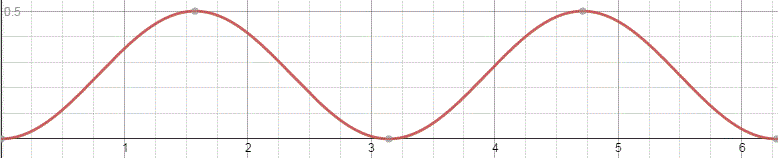
In the example we chose, we didn’t need to worry about space. It was all about time: an evolving state over time. We also knew the answers we wanted to get: if there is some probability for the system to ‘flip’ from one state to another, we know it will, at some point in time. We also want probabilities to add up to one, so we knew the graph below had to be the result we would find: if our molecule can be in two states only, and it starts of in one, then the probability that it will remain in that state will gradually decline, while the probability that it flips into the other state will gradually increase, which is what is depicted below.

However, the graph above is only a Platonic idea: we don’t bother to actually verify what state the molecule is in. If we did, we’d have to ‘re-set’ our t = 0 point, and start all over again. The wavefunction would collapse, as they say, because we’ve made a measurement. However, having said that, yes, in the physicist’s Platonic world of ideas, the probability functions above make perfect sense. They are beautiful. You should note, for example, that P₁ (i.e. the probability to be in state 1) and P₂ (i.e. the probability to be in state 2) add up to 1 all of the time, so we don’t need to integrate over a cycle or something: so it’s all perfect!

These probability functions are based on ideas that are even more Platonic: interfering amplitudes. Let me explain.

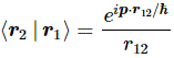
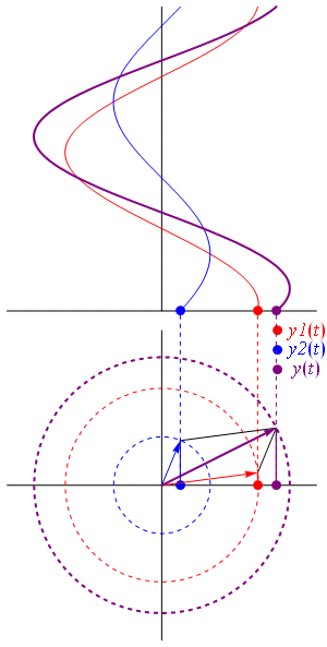
Quantum physics is based on the idea that these probabilities are determined by some wavefunction, a complex-valued amplitude that varies in time and space. It’s a two-dimensional thing, and then it’s not. It’s two-dimensional because it combines a sine and cosine, i.e. a real and an imaginary part, but the argument of the sine and the cosine is the same, and the sine and cosine are the same function, except for a phase shift equal to π. We write:

a·e^−iθ= a·cos(θ) – a·sin(−θ) = a·cosθ – a·sinθ

The minus sign is there because it turns out that Nature measures angles, i.e. our phase, clockwise, rather than counterclockwise, so that’s not as per our mathematical convention. But that’s a minor detail, really. [It should give you some food for thought, though.] For the rest, the related graph is as simple as the formula:

Now, the phase of this wavefunction is written as θ = (ω·t − k ∙x). Hence, ω determines how this wavefunction varies in time, and the wavevector k tells us how this wave varies in space. The young Frenchman Comte Louis de Broglie noted the mathematical similarity between the ω·t − k ∙x expression and Einstein’s four-vector product p_μx_μ= E·t − p∙x, which remains invariant under a Lorentz transformation. He also understood that the Planck-Einstein relation E = ħ·ω actually defines the energy unit and, therefore, that any frequency, any oscillation really, in space or in time, is to be expressed in terms of ħ.

[To be precise, the fundamental quantum of energy is h = ħ·2π, because that’s the energy of one cycle. To illustrate the point, think of the Planck-Einstein relation. It gives us the energy of a photon with frequency f: E_γ = h·f. If we re-write this equation as E_γ/f = h, and we do a dimensional analysis, we get: h = E_γ/f ⇔ 6.626×10⁻³⁴ joule·second = [x joule]/[f cycles per second] ⇔ h = 6.626×10⁻³⁴ joule per cycle. It’s only because we are expressing ω and k as angular frequencies (i.e. in radians per second or per meter, rather than in cycles per second or per meter) that we have to think of ħ = h/2π rather than h.]

Louis de Broglie connected the dots between some other equations too. He was fully familiar with the equations determining the phase and group velocity of composite waves, or a wavetrain that actually might represent a wavicle traveling through spacetime. In short, he boldly equated ω with ω = E/ħ and k with k = p/ħ, and all came out alright. It made perfect sense!

I’ve written enough about this. What I want to write about here is how this also makes for the situation on hand: a simple two-state system that depends on time only. So its phase is θ = ω·t = E₀/ħ. What’s E₀? It is the total energy of the system, including the equivalent energy of the particle’s rest mass and any potential energy that may be there because of the presence of one or the other force field. What about kinetic energy? Well… We said it: in this case, there is no translational or linear momentum, so p = 0. So our Platonic wavefunction reduces to:

a·e^−iθ= ae⁻⁽^{i/ħ)·(E₀·t)}

Great! […] But… Well… No! The problem with this wavefunction is that it yields a constant probability. To be precise, when we take the absolute square of this wavefunction – which is what we do when calculating a probability from a wavefunction − we get P = a², always. The ‘normalization’ condition (so that’s the condition that probabilities have to add up to one) implies that P₁ = P₂ = a² = 1/2. Makes sense, you’ll say, but the problem is that this doesn’t reflect reality: these probabilities do not evolve over time and, hence, our ammonia molecule never ‘flips’ its spin direction from ‘up’ to ‘down’, or vice versa. In short, our wavefunction does not explain reality.

The problem is not unlike the problem we’d had with a similar function relating the momentum and the position of a particle. You’ll remember it: we wrote it as a·e^−iθ= ae⁽^{i/ħ)·(p·x)}. [Note that we can write a·e^−iθ= a·e⁻⁽^{i/ħ)·(E₀·t − p·x)}= a·e⁻⁽ⁱ^/ħ)·(E^₀·t)·e⁽^{i/ħ)·(p·x)}, so we can always split our wavefunction in a ‘time’ and a ‘space’ part.] But then we found that this wavefunction also yielded a constant and equal probability all over space, which implies our particle is everywhere (and, therefore, nowhere, really).

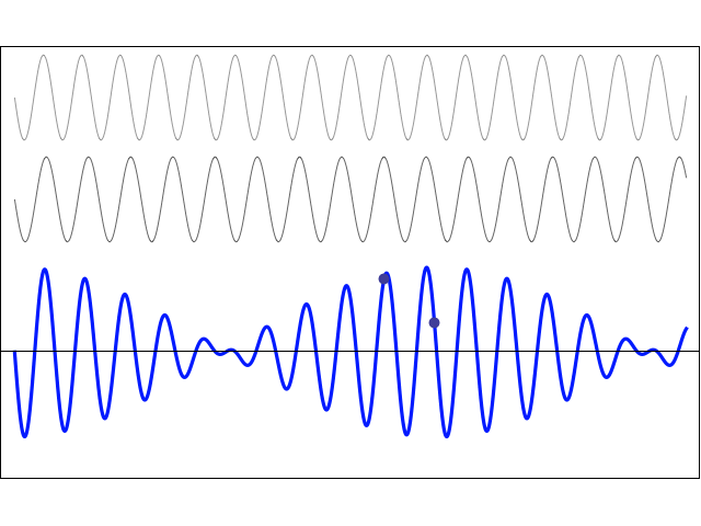
In quantum physics, this problem is solved by introducing uncertainty. Introducing some uncertainty about the energy, or about the momentum, is mathematically equivalent to saying that we’re actually looking at a composite wave, i.e. the sum of a finite or infinite set of component waves. So we have the same ω = E/ħ and k = p/ħ relations, but we apply them to n energy levels, or to some continuous range of energy levels ΔE. It amounts to saying that our wave function doesn’t have a specific frequency: it now has n frequencies, or a range of frequencies Δω = ΔE/ħ.

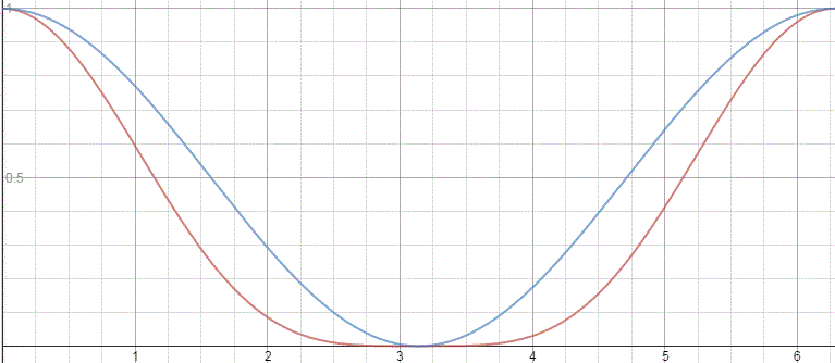
We know what that does: it ensures our wavefunction is being ‘contained’ in some ‘envelope’. It becomes a wavetrain, or a kind of beat note, as illustrated below:

[The animation also shows the difference between the group and phase velocity: the green dot shows the group velocity, while the red dot travels at the phase velocity.]

This begs the following question: what’s the uncertainty really? Is it an uncertainty in the energy, or is it an uncertainty in the wavefunction? I mean: we have a function relating the energy to a frequency. Introducing some uncertainty about the energy is mathematically equivalent to introducing uncertainty about the frequency. Of course, the answer is: the uncertainty is in both, so it’s in the frequency and in the energy and both are related through the wavefunction. So… Well… Yes. In some way, we’re chasing our own tail. 🙂

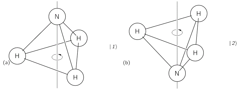
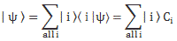
However, the trick does the job, and perfectly so. Let me summarize what we did in the previous post: we had the ammonia molecule, i.e. an NH₃ molecule, with the nitrogen ‘flipping’ across the hydrogens from time to time, as illustrated below:

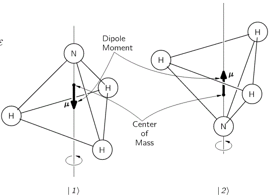
This ‘flip’ requires energy, which is why we associate two energy levels with the molecule, rather than just one. We wrote these two energy levels as E₀+ A and E₀− A. That assumption solved all of our problems. [Note that we don’t specify what the energy barrier really consists of: moving the center of mass obviously requires some energy, but it is likely that a ‘flip’ also involves overcoming some electrostatic forces, as shown by the reversal of the electric dipole moment in the illustration above.] To be specific, it gave us the following wavefunctions for the amplitude to be in the ‘up’ or ‘1’ state versus the ‘down’ or ‘2’ state respectivelly:

C₁= (1/2)·e^{−(i/ħ)·(E₀− A)·t}+ (1/2)·e^{−(i/ħ)·(E₀+ A)·t}
C₂= (1/2)·e^{−(i/ħ)·(E₀− A)·t}– (1/2)·e^{−(i/ħ)·(E₀+ A)·t}

Both are composite waves. To be precise, they are the sum of two component waves with a temporal frequency equal to ω₁= (E₀− A)/ħ and ω₁= (E₀+ A)/ħ respectively. [As for the minus sign in front of the second term in the wave equation for C₂, −1 = e^±iπ, so + (1/2)·e^{−(i/ħ)·(E₀+ A)·t}and – (1/2)·e^{−(i/ħ)·(E₀+ A)·t} are the same wavefunction: they only differ because their relative phase is shifted by ±π.] So the so-called base states of the molecule themselves are associated with two different energy levels: it’s not like one state has more energy than the other.

You’ll say: so what?

Well… Nothing. That’s it really. That’s all I wanted to say here. The absolute square of those two wavefunctions gives us those time-dependent probabilities above, i.e. the graph we started this post with. So… Well… Done!

You’ll say: where’s the ‘envelope’? Oh! Yes! Let me tell you. The C₁(t) and C₂(t) equations can be re-written as:

Now, remembering our rules for adding and subtracting complex conjugates (e^iθ + e^–iθ = 2cosθ and e^iθ − e^–iθ = 2sinθ), we can re-write this as:

So there we are! We’ve got wave equations whose temporal variation is basically defined by E₀but, on top of that, we have an envelope here: the cos(A·t/ħ) and sin(A·t/ħ) factor respectively. So their magnitude is no longer time-independent: both the phase as well as the amplitude now vary with time. The associated probabilities are the ones we plotted:

|C₁(t)|²= cos²[(A/ħ)·t], and
|C₂(t)|²= sin²[(A/ħ)·t].

So, to summarize it all once more, allowing the nitrogen atom to push its way through the three hydrogens, so as to flip to the other side, thereby breaking the energy barrier, is equivalent to associating two energy levels to the ammonia molecule as a whole, thereby introducing some uncertainty, or indefiniteness as to its energy, and that, in turn, gives us the amplitudes and probabilities that we’ve just calculated. [And you may want to note here that the probabilities “sloshing back and forth”, or “dumping into each other” – as Feynman puts it – is the result of the varying magnitudes of our amplitudes, so that’s the ‘envelope’ effect. It’s only because the magnitudes vary in time that their absolute square, i.e. the associated probability, varies too.

So… Well… That’s it. I think this and all of the previous posts served as a nice introduction to quantum physics. More in particular, I hope this post made you appreciate the mathematical framework is not as horrendous as it often seems to be.

When thinking about it, it’s actually all quite straightforward, and it surely respects Occam’s principle of parsimony in philosophical and scientific thought, also know as Occam’s Razor: “When trying to explain something, it is vain to do with more what can be done with less.” So the math we need is the math we need, really: nothing more, nothing less. As I’ve said a couple of times already, Occam would have loved the math behind QM: the physics call for the math, and the math becomes the physics.

That’s what makes it beautiful. 🙂

Post scriptum:

One might think that the addition of a term in the argument in itself would lead to a beat note and, hence, a varying probability but, no! We may look at e^{−(i/ħ)·(E₀+ A)·t}as a product of two amplitudes:

e^{−(i/ħ)·(E₀+ A)·t}= e^{−(i/ħ)·E₀·t}·e^{−(i/ħ)·A·t}

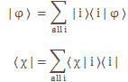
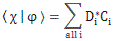
But, when writing this all out, one just gets a cos(α·t+β·t)–sin(α·t+β·t), whose absolute square |cos(α·t+β·t)–sin(α·t+β·t)|²= 1. However, writing e^{−(i/ħ)·(E₀+ A)·t}as a product of two amplitudes in itself is interesting. We multiply amplitudes when an event consists of two sub-events. For example, the amplitude for some particle to go from s to x via some point a is written as:

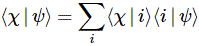
〈 x | s 〉_{via a} = 〈 x | a 〉〈 a | s 〉

Having said that, the graph of the product is uninteresting: the real and imaginary part of the wavefunction are a simple sine and cosine function, and their absolute square is constant, as shown below.

Adding two waves with very different frequencies – A is a fraction of E₀– gives a much more interesting pattern, like the one below, which shows an e^−iαt+e^−iβt= cos(αt)−i·sin(αt)+cos(βt)−i·sin(βt) = cos(αt)+cos(βt)−i·[sin(αt)+sin(βt)] pattern for α = 1 and β = 0.1.

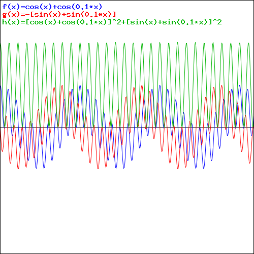
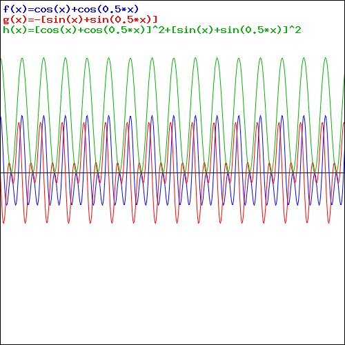
That doesn’t look a beat note, does it? The graphs below, which use 0.5 and 0.01 for β respectively, are not typical beat notes either.

We get our typical ‘beat note’ only when we’re looking at a wave traveling in space, so then we involve the space variable x again, and the relations that come with in, i.e. a phase velocity v_p= ω/k = (E/ħ)/(p/ħ) = E/p = c²/v (read: all component waves travel at the same speed), and a group velocity v_g= dω/dk = v (read: the composite wave or wavetrain travels at the classical speed of our particle, so it travels with the particle, so to speak). That’s what’s I’ve shown numerous times already, but I’ll insert one more animation here, just to make sure you see what we’re talking about. [Credit for the animation goes to another site, one on acoustics, actually!]

So what’s left? Nothing much. The only thing you may want to do is to continue thinking about that wavefunction. It’s tempting to think it actually is the particle, somehow. But it isn’t. So what is it then? Well… Nobody knows, really, but I like to think it does travel with the particle. So it’s like a fundamental property of the particle. We need it every time when we try to measure something: its position, its momentum, its spin (i.e. angular momentum) or, in the example of our ammonia molecule, its orientation in space. So the funny thing is that, in quantum mechanics,

We can measure probabilities only, so there’s always some randomness. That’s how Nature works: we don’t really know what’s happening. We don’t know the internal wheels and gears, so to speak, or the ‘hidden variables’, as one interpretation of quantum mechanics would say. In fact, the most commonly accepted interpretation of quantum mechanics says there are no ‘hidden variables’.
But then, as Polonius famously put, there is a method in this madness, and the pioneers – I mean Werner Heisenberg, Louis de Broglie, Niels Bohr, Paul Dirac, etcetera – discovered. All probabilities can be found by taking the square of the absolute value of a complex-valued wavefunction (often denoted by Ψ), whose argument, or phase (θ), is given by the de Broglie relations ω = E/ħ and k = p/ħ:

θ = (ω·t − k ∙x) = (E/ħ)·t − (p/ħ)·x

That should be obvious by now, as I’ve written dozens of posts on this by now. 🙂 I still have trouble interpreting this, however—and I am not ashamed, because the Great Ones I just mentioned have trouble with that too. But let’s try to go as far as we can by making a few remarks:

Adding two terms in math implies the two terms should have the same dimension: we can only add apples to apples, and oranges to oranges. We shouldn’t mix them. Now, the (E/ħ)·t and (p/ħ)·x terms are actually dimensionless: they are pure numbers. So that’s even better. Just check it: energy is expressed in newton·meter (force over distance, remember?) or electronvolts (1 eV = 1.6×10⁻¹⁹J = 1.6×10⁻¹⁹N·m); Planck’s constant, as the quantum of action, is expressed in J·s or eV·s; and the unit of (linear) momentum is 1 N·s = 1 kg·m/s = 1 N·s. E/ħ gives a number expressed per second, and p/ħ a number expressed per meter. Therefore, multiplying it by t and x respectively gives us a dimensionless number indeed.
It’s also an invariant number, which means we’ll always get the same value for it. As mentioned above, that’s because the four-vector product p_μx_μ= E·t − p∙x is invariant: it doesn’t change when analyzing a phenomenon in one reference frame (e.g. our inertial reference frame) or another (i.e. in a moving frame).
Now, Planck’s quantum of action h or ħ (they only differ in their dimension: h is measured in cycles per second and ħ is measured in radians per second) is the quantum of energy really. Indeed, if “energy is the currency of the Universe”, and it’s real and/or virtual photons who are exchanging it, then it’s good to know the currency unit is h, i.e. the energy that’s associated with one cycle of a photon.
It’s not only time and space that are related, as evidenced by the fact that t − x itself is an invariant four-vector, E and p are related too, of course! They are related through the classical velocity of the particle that we’re looking at: E/p = c²/v and, therefore, we can write: E·β = p·c, with β = v/c, i.e. the relative velocity of our particle, as measured as a ratio of the speed of light. Now, I should add that the t − x four-vector is invariant only if we measure time and space in equivalent units. Otherwise, we have to write c·t − x. If we do that, so our unit of distance becomes c meter, rather than one meter, or our unit of time becomes the time that is needed for light to travel one meter, then c = 1, and the E·β = p·c becomes E·β = p, which we also write as β = p/E: the ratio of the energy and the momentum of our particle is its (relative) velocity.

Combining all of the above, we may want to assume that we are measuring energy and momentum in terms of the Planck constant, i.e. the ‘natural’ unit for both. In addition, we may also want to assume that we’re measuring time and distance in equivalent units. Then the equation for the phase of our wavefunctions reduces to:

θ = (ω·t − k ∙x) = E·t − p·x

Now, θ is the argument of a wavefunction, and we can always re-scale such argument by multiplying or dividing it by some constant. It’s just like writing the argument of a wavefunction as v·t–x or (v·t–x)/v = t –x/v with v the velocity of the waveform that we happen to be looking at. [In case you have trouble following this argument, please check the post I did for my kids on waves and wavefunctions.] Now, the energy conservation principle tells us the energy of a free particle won’t change. [Just to remind you, a ‘free particle’ means it is present in a ‘field-free’ space, so our particle is in a region of uniform potential.] You see what I am going to do now: we can, in this case, treat E as a constant, and divide E·t − p·x by E, so we get a re-scaled phase for our wavefunction, which I’ll write as:

φ = (E·t − p·x)/E = t − (p/E)·x = t − β·x

Now that’s the argument of a wavefunction with the argument expressed in distance units. Alternatively, we could also look at p as some constant, as there is no variation in potential energy that will cause a change in momentum, i.e. in kinetic energy. We’d then divide by p and we’d get (E·t − p·x)/p = (E/p)·t − x) = t/β − x, which amounts to the same, as we can always re-scale by multiplying it with β, which would then yield the same t − β·x argument.

The point is, if we measure energy and momentum in terms of the Planck unit (I mean: in terms of the Planck constant, i.e. the quantum of energy), and if we measure time and distance in ‘natural’ units too, i.e. we take the speed of light to be unity, then our Platonic wavefunction becomes as simple as:

Φ(φ) = a·e^−iφ= a·e^{−i(t − β·x)}

This is a wonderful formula, but let me first answer your most likely question: why would we use a relative velocity?Well… Just think of it: when everything is said and done, the whole theory of relativity and, hence, the whole of physics, is based on one fundamental and experimentally verified fact: the speed of light is absolute. In whatever reference frame, we will always measure it as 299,792,458 m/s. That’s obvious, you’ll say, but it’s actually the weirdest thing ever if you start thinking about it, and it explains why those Lorentz transformations look so damn complicated. In any case, this fact legitimately establishes c as some kind of absolute measure against which all speeds can be measured. Therefore, it is only natural indeed to express a velocity as some number between 0 and 1. Now that amounts to expressing it as the β = v/c ratio.

Let’s now go back to that Φ(φ) = a·e^−iφ= a·e^{−i(t − β·x)}wavefunction. Its temporal frequency ω is equal to one, and its spatial frequency k is equal to β = v/c. It couldn’t be simpler but, of course, we’ve got this remarkably simple result because we re-scaled the argument of our wavefunction using the energy and momentum itself as the scale factor. So, yes, we can re-write the wavefunction of our particle in a particular elegant and simple form using the only information that we have when looking at quantum-mechanical stuff: energy and momentum, because that’s what everything reduces to at that level.

Of course, the analysis above does not include uncertainty. Our information on the energy and the momentum of our particle will be incomplete: we’ll write E = E₀± σ_E, and p = p₀± σ_p. [I am a bit tired of using the Δ symbol, so I am using the σ symbol here, which denotes a standard deviation of some density function. It underlines the probabilistic, or statistical, nature of our approach.] But, including that, we’ve pretty much explained what quantum physics is about here.

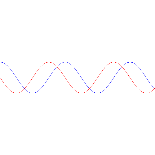
You just need to get used to that complex exponential: e^−iφ = cos(−φ) + i·sin(−φ) = cos(φ) − i·sin(φ). Of course, it would have been nice if Nature would have given us a simple sine or cosine function. [Remember the sine and cosine function are actually the same, except for a phase difference of 90 degrees: sin(φ) = cos(π/2−φ) = cos(φ+π/2). So we can go always from one to the other by shifting the origin of our axis.] But… Well… As we’ve shown so many times already, a real-valued wavefunction doesn’t explain the interference we observe, be it interference of electrons or whatever other particles or, for that matter, the interference of electromagnetic waves itself, which, as you know, we also need to look at as a stream of photons , i.e. light quanta, rather than as some kind of infinitely flexible aether that’s undulating, like water or air.

So… Well… Just accept that e^−iφ is a very simple periodic function, consisting of two sine waves rather than just one, as illustrated below.

And then you need to think of stuff like this (the animation is taken from Wikipedia), but then with a projection of the sine of those phasors too. It’s all great fun, so I’ll let you play with it now. 🙂

Some content on this page was disabled on June 20, 2020 as a result of a DMCA takedown notice from Michael A. Gottlieb, Rudolf Pfeiffer, and The California Institute of Technology. You can learn more about the DMCA here:

https://wordpress.com/support/copyright-and-the-dmca/
Some content on this page was disabled on June 20, 2020 as a result of a DMCA takedown notice from Michael A. Gottlieb, Rudolf Pfeiffer, and The California Institute of Technology. You can learn more about the DMCA here:

https://wordpress.com/support/copyright-and-the-dmca/

The Hamiltonian for a two-state system: the ammonia example

Ammonia, i.e. NH₃, is a colorless gas with a strong smell. Its serves as a precursor in the production of fertilizer, but we also know it as a cleaning product, ammonium hydroxide, which is NH₃ dissolved in water. It has a lot of other uses too. For example, its use in this post, is to illustrate a two-state system. 🙂 We’ll apply everything we learned in our previous posts and, as I mentioned when finishing the last of those rather mathematical pieces, I think the example really feels like a reward after all of the tough work on all of those abstract concepts – like that Hamiltonian matrix indeed – so I hope you enjoy it. So… Here we go!

The geometry of the NH₃ molecule can be described by thinking of it as a trigonal pyramid, with the nitrogen atom (N) at its apex, and the three hydrogen atoms (H) at the base, as illustrated below. [Feynman’s illustration is slightly misleading, though, because it may give the impression that the hydrogen atoms are bonded together somehow. That’s not the case: the hydrogen atoms share their electron with the nitrogen, thereby completing the outer shell of both atoms. This is referred to as a covalent bond. You may want to look it up, but it is of no particular relevance to what follows here.]

Here, we will only worry about the spin of the molecule about its axis of symmetry, as shown above, which is either in one direction or in the other, obviously. So we’ll discuss the molecule as a two-state system. So we don’t care about its translational (i.e. linear) momentum, its internal vibrations, or whatever else that might be going on. It is one of those situations illustrating that the spin vector, i.e. the vector representing angular momentum, is an axial vector: the first state, which is denoted by | 1 〉 is not the mirror image of state | 2 〉. In fact, there is a more sophisticated version of the illustration above, which usefully reminds us of the physics involved.

It should be noted, however, that we don’t need to specify what the energy barrier really consists of: moving the center of mass obviously requires some energy, but it is likely that a ‘flip’ also involves overcoming some electrostatic forces, as shown by the reversal of the electric dipole moment in the illustration above. In fact, the illustration may confuse you, because we’re usually thinking about some net electric charge that’s spinning, and so the angular momentum results in a magnetic dipole moment, that’s either ‘up’ or ‘down’, and it’s usually also denoted by the very same μ symbol that’s used below. As I explained in my post on angular momentum and the magnetic moment, it’s related to the angular momentum J through the so-called g-number. In the illustration above, however, the μ symbol is used to denote an electric dipole moment, so that’s different. Don’t rack your brain over it: just accept there’s an energy barrier, and it requires energy to get through it. Don’t worry about its details!

Indeed, in quantum mechanics, we abstract away from such nitty-gritty, and so we just say that we have base states | i 〉 here, with i equal to 1 or 2. One or the other. Now, in our post on quantum math, we introduced what Feynman only half-jokingly refers to as the Great Law of Quantum Physics: | = ∑ | i 〉〈 i | over all base states i. It basically means that we should always describe our initial and end states in terms of base states. Applying that principle to the state of our ammonia molecule, which we’ll denote by | ψ 〉, we can write:

You may – in fact, you should – mechanically apply that | = ∑ | i 〉〈 i | substitution to | ψ 〉 to get what you get here, but you should also think about what you’re writing. It’s not an easy thing to interpret, but it may help you to think of the similarity of the formula above with the description of a vector in terms of its base vectors, which we write as A = A_x·e₁+ A_y·e₂ + A_z·e₃. Just substitute the A_icoefficients for C_i and the e_ibase vectors for the | i 〉 base states, and you may understand this formula somewhat better. It also explains why the | ψ 〉 state is often referred to as the | ψ 〉 state vector: unlike our A = ∑ A_i·e_isum of base vectors, our | 1 〉 C₁ + | 2 〉 C₂sum does not have any geometrical interpretation but… Well… Not all ‘vectors’ in math have a geometric interpretation, and so this is a case in point.

It may also help you to think of the time-dependency. Indeed, this formula makes a lot more sense when realizing that the state of our ammonia molecule, and those coefficients C_i, depend on time, so we write: ψ = ψ(t) and C_i= C_i(t). Hence, if we would know, for sure, that our molecule is always in state | 1 〉, then C₁ = 1 and C₂ = 0, and we’d write: | ψ 〉 = | 1 〉 = | 1 〉 1 + | 2 〉 0. [I am always tempted to insert a little dot (·), and change the order of the factors, so as to show we’re talking some kind of product indeed – so I am tempted to write | ψ 〉 = C₁·| 1 〉 C₁ + C₂·| 2 〉 C₂, but I note that’s not done conventionally, so I won’t do it either.]

Why this time dependency? It’s because we’ll allow for the possibility of the nitrogen to push its way through the pyramid – through the three hydrogens, really – and flip to the other side. It’s unlikely, because it requires a lot of energy to get half-way through (we’ve got what we referred to as an energy barrier here), but it may happen and, as we’ll see shortly, it results in us having to think of the the ammonia molecule as having two separate energy levels, rather than just one. We’ll denote those energy levels as E₀ ± A. However, I am getting ahead of myself here, so let me get back to the main story.

To fully understand the story, you should really read my previous post on the Hamiltonian, which explains how those C_i coefficients, as a function of time, can be determined. They’re determined by a set of differential equations (i.e. equations involving a function and the derivative of that function) which we wrote as:

If we have two base states only – which is the case here – then this set of equations is:

Two equations and two functions – C₁= C₁(t) and C₂= C₂(t) – so we should be able to solve this thing, right? Well… No. We don’t know those H_ijcoefficients. As I explained in my previous post, they also evolve in time, so we should write them as H_ij(t) instead of H_ijtout court, and so it messes the whole thing up. We have two equations and six functions really. There is no way we can solve this! So how do we get out of this mess?

Well… By trial and error, I guess. 🙂 Let us just assume the molecule would behave nicely—which we know it doesn’t, but so let’s push the ‘classical’ analysis as far as we can, so we might get some clues as to how to solve this problem. In fact, our analysis isn’t ‘classical’ at all, because we’re still talking amplitudes here! However, you’ll agree the ‘simple’ solution would be that our ammonia molecule doesn’t ‘tunnel’. It just stays in the same spin direction forever. Then H₁₂and H₂₁must be zero (think of the U₁₂(t + Δt, t) and U₂₁(t + Δt, t) functions) and H₁₁and H₂₂are equal to… Well… I’d love to say they’re equal to 1 but… Well… You should go through my previous posts: these Hamiltonian coefficients are related to probabilities but… Well… Same-same but different, as they say in Asia. 🙂 They’re amplitudes, which are things you use to calculate probabilities. But calculating probabilities involve normalization and other stuff, like allowing for interference of amplitudes, and so… Well… To make a long story short, if our ammonia molecule would stay in the same spin direction forever, then H₁₁and H₂₂are not one but some constant. In any case, the point is that they would not change in time (so H₁₁(t) = H₁₁ and H₂₂(t ) = H₂₂), and, therefore, our two equations would reduce to:

So the coefficients are now proper coefficients, in the sense that they’ve got some definite value, and so we have two equations and two functions only now, and so we can solve this. Indeed, remembering all of the stuff we wrote on the magic of exponential functions (more in particular, remembering that d[e^x]/dx), we can understand the proposed solution:

As Feynman notes: “These are just the amplitudes for stationary states with the energies E₁= H₁₁ and E₂= H₂₂.” Now let’s think about that. Indeed, I find the term ‘stationary’ state quite confusing, as it’s ill-defined. In this context, it basically means that we have a wavefunction that is determined by (i) a definite (i.e. unambiguous, or precise) energy level and (ii) that there is no spatial variation. Let me refer you to my post on the basics of quantum math here. We often use a sort of ‘Platonic’ example of the wavefunction indeed:

a·e^−i·θ= e^{−i·(ω·t − k ∙x)} = a·e^{−(i/ħ)·(E·t − p∙x)}

So that’s a wavefunction assuming the particle we’re looking at has some well-defined energy E and some equally well-defined momentum p. Now, that’s kind of ‘Platonic’ indeed, because it’s more like an idea, rather than something real. Indeed, a wavefunction like that means that the particle is everywhere and nowhere, really—because its wavefunction is spread out all of over space. Of course, we may think of the ‘space’ as some kind of confined space, like a box, and then we can think of this particle as being ‘somewhere’ in that box, and then we look at the temporal variation of this function only – which is what we’re doing now: we don’t consider the space variable x at all. So then the equation reduces to a·e^{–(i/ħ)·(E·t)}, and so… Well… Yes. We do find that our Hamiltonian coefficient H_iiis like the energy of the | i 〉 state of our NH₃ molecule, so we write: H₁₁= E₁, and H₂₂= E₂, and the ‘wavefunctions’ of our C₁and C₂coefficients can be written as:

C₁= a·e^{−(i/ħ)·(H₁₁·t)}= a·e^{−(i/ħ)·(E₁·t)}, with H₁₁= E₁, and
C₂= a·e^{−(i/ħ)·(H₂₂·t)}= a·e^{−(i/ħ)·(E₂·t)}, with H₂₂= E₂.

But can we interpret C₁and C₂as proper amplitudes? They are just coefficients in these equations, aren’t they? Well… Yes and no. From what we wrote in previous posts, you should remember that these C_icoefficients are equal to 〈 i | ψ 〉, so they are the amplitude to find our ammonia molecule in one state or the other.

Back to Feynman now. He adds, logically but brilliantly:

“We note, however, that for the ammonia molecule the two states |1〉 and |2〉 have a definite symmetry. If nature is at all reasonable, the matrix elements H₁₁ and H₂₂ must be equal. We’ll call them both E₀, because they correspond to the energy the states would have if H₁₁ and H₂₂ were zero.”

So our C₁and C₂amplitudes then reduce to:

C₁= 〈 1 | ψ 〉 = a·e^{−(i/ħ)·(E₀·t)}
C₂=〈 2 | ψ 〉 = a·e^{−(i/ħ)·(E₀·t)}

We can now take the absolute square of both to find the probability for the molecule to be in state 1 or in state 2:

|〈 1 | ψ 〉|²= |a·e^{−(i/ħ)·(E₀·t)}|²= a²
|〈 2 | ψ 〉|²= |a·e^{−(i/ħ)·(E₀·t)}|²= a²

Now, the probabilities have to add up to 1, so a²+ a²= 1 and, therefore, the probability to be in either in state 1 or state 2 is 0.5, which is what we’d expect.

Note: At this point, it is probably good to get back to our | ψ 〉 = | 1 〉 C₁ + | 2 〉 C₂equation, so as to try to understand what it really says. Substituting the a·e^{−(i/ħ)·(E₀·t)} expression for C₁ and C₂yields:

| ψ 〉 = | 1 〉 a·e^{−(i/ħ)·(E₀·t)} + | 2 〉 a·e^{−(i/ħ)·(E₀·t)}= [| 1 〉 + | 2 〉] a·e^{−(i/ħ)·(E₀·t)}

Now, what is this saying, really? In our previous post, we explained this is an ‘open’ equation, so it actually doesn’t mean all that much: we need to ‘close’ or ‘complete’ it by adding a ‘bra’, i.e. a state like 〈 χ |, so we get a 〈 χ | ψ〉 type of amplitude that we can actually do something with. Now, in this case, our final 〈 χ | state is either 〈 1 | or 〈 2 |, so we write:

〈 1 | ψ 〉 = [〈 1 | 1 〉 + 〈 1 | 2 〉]·a·e^{−(i/ħ)·(E₀·t)}= [1 + 0]·a·e^{−(i/ħ)·(E₀·t)}· = a·e^{−(i/ħ)·(E₀·t)}
〈 2 | ψ 〉 = [〈 2 | 1 〉 + 〈 2 | 2 〉]·a·e^{−(i/ħ)·(E₀·t)}= [0 + 1]·a·e^{−(i/ħ)·(E₀·t)}· = a·e^{−(i/ħ)·(E₀·t)}

Note that I finally added the multiplication dot (·) because we’re talking proper amplitudes now and, therefore, we’ve got a proper product too: we multiply one complex number with another. We can now take the absolute square of both to find the probability for the molecule to be in state 1 or in state 2:

|〈 1 | ψ 〉|²= |a·e^{−(i/ħ)·(E₀·t)}|²= a²
|〈 2 | ψ 〉|²= |a·e^{−(i/ħ)·(E₀·t)}|²= a²

Unsurprisingly, we find the same thing: these probabilities have to add up to 1, so a²+ a²= 1 and, therefore, the probability to be in state 1 or state 2 is 0.5. So the notation and the logic behind makes perfect sense. But let me get back to the lesson now.

The point is: the true meaning of a ‘stationary’ state here, is that we have non-fluctuating probabilities. So they are and remain equal to some constant, i.e. 1/2 in this case. This implies that the state of the molecule does not change: there is no way to go from state 1 to state 2 and vice versa. Indeed, if we know the molecule is in state 1, it will stay in that state. [Think about what normalization of probabilities means when we’re looking at one state only.]

You should note that these non-varying probabilities are related to the fact that the amplitudes have a non-varying magnitude. The phase of these amplitudes varies in time, of course, but their magnitude is and remains a, always. The amplitude is not being ‘enveloped’ by another curve, so to speak.

OK. That should be clear enough. Sorry I spent so much time on this, but this stuff on ‘stationary’ states comes back again and again and so I just wanted to clear that up as much as I can. Let’s get back to the story.

So we know that, what we’re describing above, is not what ammonia does really. As Feynman puts it: “The equations [i.e. the C₁and C₂equations above] don’t tell us what what ammonia really does. It turns out that it is possible for the nitrogen to push its way through the three hydrogens and flip to the other side. It is quite difficult; to get half-way through requires a lot of energy. How can it get through if it hasn’t got enough energy? There is some amplitude that it will penetrate the energy barrier. It is possible in quantum mechanics to sneak quickly across a region which is illegal energetically. There is, therefore, some [small] amplitude that a molecule which starts in |1〉 will get to the state |2〉. The coefficients H₁₂ and H₂₁ are not really zero.”

He adds: “Again, by symmetry, they should both be the same—at least in magnitude. In fact, we already know that, in general, H_ijmust be equal to the complex conjugate of H_ji.”

His next step, then, is to interpreted as either a stroke of genius or, else, as unexplained. 🙂 He invokes the symmetry of the situation to boldly state that H₁₂is some real negative number, which he denotes as −A, which – because it’s a real number (so the imaginary part is zero) – must be equal to its complex conjugate H₂₁. So then Feynman does this fantastic jump in logic. First, he keeps using the E₀ value for H₁₁ and H₂₂, motivating that as follows: “If nature is at all reasonable, the matrix elements H₁₁ and H₂₂ must be equal, and we’ll call them both E₀, because they correspond to the energy the states would have if H₁₁ and H₂₂ were zero.” Second, he uses that minus A value for H₁₂and H₂₁. In short, the two equations and six functions are now reduced to:

Solving these equations is rather boring. Feynman does it as follows:

solution

Now, what does these equations actually mean? It depends on those a and b coefficients. Looking at the solutions, the most obvious question to ask is: what if a or b are zero? If b is zero, then the second terms in both equations is zero, and so C₁ and C₂ are exactly the same: two amplitudes with the same temporal frequency ω = (E₀− A)/ħ. If a is zero, then C₁ and C₂ are the same too, but with opposite sign: two amplitudes with the same temporal frequency ω = (E₀+ A)/ħ. Squaring them – in both cases (i.e. for a = 0 or b = 0) – yields, once again, an equal and constant probability for the spin of the ammonia molecule to in the ‘up’ or ‘down’ or ‘down’. To be precise, we We can now take the absolute square of both to find the probability for the molecule to be in state 1 or in state 2:

For b = 0: |〈 1 | ψ 〉|²= |(a/2)·e^{−(i/ħ)·(E₀− A)·t}|²= a²/4 = |〈 2 | ψ 〉|²
For a = 0: |〈 1 | ψ 〉|²=|(b/2)·e^{−(i/ħ)·(E₀+ A)·t}|²= b²/4 = |〈 2 | ψ 〉|²(the minus sign in front of b/2 is squared away)

So we get two stationary states now. Why two instead of one? Well… You need to use your imagination a bit here. They actually reflect each other: they’re the same as the one stationary state we found when assuming our nitrogen atom could not ‘flip’ from one position to the other. It’s just that the introduction of that possibility now results in a sort of ‘doublet’ of energy levels. But so we shouldn’t waste our time on this, as we want to analyze the general case, for which the probabilities to be in state 1 or state 2 do vary in time. So that’s when a and b are non-zero.

To analyze it all, we may want to start with equating t to zero. We then get:

This leads us to conclude that a = b = 1, so our equations for C₁(t) and C₂(t) can now be written as:

Remembering our rules for adding and subtracting complex conjugates (e^iθ + e^–iθ = 2cosθ and e^iθ − e^–iθ = 2sinθ), we can re-write this as:

Now these amplitudes are much more interesting. Their temporal variation is defined by E₀but, on top of that, we have an envelope here: the cos(A·t/ħ) and sin(A·t/ħ) factor respectively. So their magnitude is no longer time-independent: both the phase as well as the amplitude now vary with time. What’s going on here becomes quite obvious when calculating and plotting the associated probabilities, which are

|C₁(t)|²= cos²(A·t/ħ), and
|C₂(t)|²= sin²(A·t/ħ)

respectively (note that the absolute square of i is equal to 1, not −1). The graph of these functions is depicted below.

As Feynman puts it: “The probability sloshes back and forth.” Indeed, the way to think about this is that, if our ammonia molecule is in state 1, then it will not stay in that state. In fact, one can be sure the nitrogen atom is going to flip at some point in time, with the probabilities being defined by that fluctuating probability density function above. Indeed, as time goes by, the probability to be in state 2 increases, until it will effectively be in state 2. And then the cycle reverses.

Our | ψ 〉 = | 1 〉 C₁ + | 2 〉 C₂equation is a lot more interesting now, as we do have a proper mix of pure states now: we never really know in what state our molecule will be, as we have these ‘oscillating’ probabilities now, which we should interpret carefully.

The point to note is that the a = 0 and b = 0 solutions came with precise temporal frequencies: (E₀− A)/ħ and (E₀+ A)/ħ respectively, which correspond to two separate energy levels: E₀− A and E₀+ A respectively, with |A| = H₁₂= H₂₁. So everything is related to everything once again: allowing the nitrogen atom to push its way through the three hydrogens, so as to flip to the other side, thereby breaking the energy barrier, is equivalent to associating two energy levels to the ammonia molecule as a whole, thereby introducing some uncertainty, or indefiniteness as to its energy, and that, in turn, gives us the amplitudes and probabilities that we’ve just calculated.

Note that the probabilities “sloshing back and forth”, or “dumping into each other” – as Feynman puts it – is the result of the varying magnitudes of our amplitudes, going up and down and, therefore, their absolute square varies too.

So… Well… That’s it as an introduction to a two-state system. There’s more to come. Ammonia is used in the ammonia maser. Now that is something that’s interesting to analyze—both from a classical as well as from a quantum-mechanical perspective. Feynman devotes a full chapter to it, so I’d say… Well… Have a look. 🙂

Post scriptum: I must assume this analysis of the NH₃ molecule, with the nitrogen ‘flipping’ across the hydrogens, triggers a lot of questions, so let me try to answer some. Let me first insert the illustration once more, so you don’t have to scroll up:

The first thing that you should note is that the ‘flip’ involves a change in the center of mass position. So that requires energy, which is why we associate two different energy levels with the molecule: E₀+ A and E₀− A. However, as mentioned above, we don’t care about the nitty-gritty here: the energy barrier is likely to combine a number of factors, including electrostatic forces, as evidenced by the flip in the electric dipole moment, which is what the μ symbol here represents! Just note that the two energy levels are separated by an amount that’s equal to 2·A, rather than A and that, once again, it becomes obvious now why Feynman would prefer the Hamiltonian to be called the ‘energy matrix’, as its coefficients do represent specific energy levels, or differences between them! Now, that assumption yielded the following wavefunctions for C₁= 〈 1 | ψ 〉 and C₁= 〈 2 | ψ 〉:

C₁= 〈 1 | ψ 〉 = (1/2)·e^{−(i/ħ)·(E₀− A)·t}+ (1/2)·e^{−(i/ħ)·(E₀+ A)·t}
C₂= 〈 2 | ψ 〉 = (1/2)·e^{−(i/ħ)·(E₀− A)·t}– (1/2)·e^{−(i/ħ)·(E₀+ A)·t}

Now, writing things this way, rather than in terms of probabilities, makes it clear that the two base states of the molecule themselves are associated with two different energy levels, so it is not like one state has more energy than the other. It’s just that the possibility of going from one state to the other requires an uncertainty about the energy, which is reflected by the energy doublet E₀± A in the wavefunction of the base states. Now, if the wavefunction of the base states incorporates that energy doublet, then it is obvious that the state of the ammonia molecule, at any point in time, will also incorporate that energy doublet.

This triggers the following remark: what’s the uncertainty really? Is it an uncertainty in the energy, or is it an uncertainty in the wavefunction? I mean: we have a function relating the energy to a frequency. Introducing some uncertainty about the energy is mathematically equivalent to introducing uncertainty about the frequency. Think of it: two energy levels implies two frequencies, and vice versa. More in general, introducing n energy levels, or some continuous range of energy levels ΔE, amounts to saying that our wave function doesn’t have a specific frequency: it now has n frequencies, or a range of frequencies Δω = ΔE/ħ. Of course, the answer is: the uncertainty is in both, so it’s in the frequency and in the energy and both are related through the wavefunction. So… In a way, we’re chasing our own tail.

Having said that, the energy may be uncertain, but it is real. It’s there, as evidenced by the fact that the ammonia molecule behaves like an atomic oscillator: we can excite it in exactly the same way as we can excite an electron inside an atom, i.e. by shining light on it. The only difference is the photon energies: to cause a transition in an atom, we use photons in the optical or ultraviolet range, and they give us the same radiation back. To cause a transition in an ammonia molecule, we only need photons with energies in the microwave range. Here, I should quickly remind you of the frequencies and energies involved. visible light is radiation in the 400–800 terahertz range and, using the E = h·f equation, we can calculate the associated energies of a photon as 1.6 to 3.2 eV. Microwave radiation – as produced in your microwave oven – is typically in the range of 1 to 2.5 gigahertz, and the associated photon energy is 4 to 10 millionths of an eV. Having illustrated the difference in terms of the energies involved, I should add that masers and lasers are based on the same physical principle: LASER and MASER stand for Light/Micro-wave Amplification by Stimulated Emission of Radiation, respectively.

So… How shall I phrase this? There’s uncertainty, but the way we are modeling that uncertainty matters. So yes, the uncertainty in the frequency of our wavefunction and the uncertainty in the energy are mathematically equivalent, but the wavefunction has a meaning that goes much beyond that. [You may want to reflect on that yourself.]

Finally, another question you may have is why would Feynman take minus A (i.e. −A) for H₁₂ and H₂₁. Frankly, my first thought on this was that it should have something to do with the original equation for these Hamiltonian coefficients, which also has a minus sign: U_ij(t + Δt, t) = δ_ij + K_ij(t)·Δt = δ_ij − (i/ħ)·H_ij(t)·Δt. For i ≠ j, this reduces to:

U_ij(t + Δt, t) = + K_ij(t)·Δt = − (i/ħ)·H_ij(t)·Δt

However, the answer is: it really doesn’t matter. One could write: H₁₂ and H₂₁ = +A, and we’d find the same equations. We’d just switch the indices 1 and 2, and the coefficients a and b. But we get the same solutions. You can figure that out yourself. Have fun with it !

Oh ! And please do let me know if some of the stuff above would trigger other questions. I am not sure if I’ll be able to answer them, but I’ll surely try, and good question always help to ensure we sort of ‘get’ this stuff in a more intuitive way. Indeed, when everything is said and done, the goal of this blog is not simply re-produce stuff, but to truly ‘get’ it, as good as we can. 🙂

Some content on this page was disabled on June 16, 2020 as a result of a DMCA takedown notice from The California Institute of Technology. You can learn more about the DMCA here:

https://wordpress.com/support/copyright-and-the-dmca/
Some content on this page was disabled on June 16, 2020 as a result of a DMCA takedown notice from The California Institute of Technology. You can learn more about the DMCA here:

https://wordpress.com/support/copyright-and-the-dmca/
Some content on this page was disabled on June 16, 2020 as a result of a DMCA takedown notice from The California Institute of Technology. You can learn more about the DMCA here:

https://wordpress.com/support/copyright-and-the-dmca/
Some content on this page was disabled on June 16, 2020 as a result of a DMCA takedown notice from The California Institute of Technology. You can learn more about the DMCA here:

https://wordpress.com/support/copyright-and-the-dmca/
Some content on this page was disabled on June 17, 2020 as a result of a DMCA takedown notice from Michael A. Gottlieb, Rudolf Pfeiffer, and The California Institute of Technology. You can learn more about the DMCA here:

https://wordpress.com/support/copyright-and-the-dmca/
Some content on this page was disabled on June 17, 2020 as a result of a DMCA takedown notice from Michael A. Gottlieb, Rudolf Pfeiffer, and The California Institute of Technology. You can learn more about the DMCA here:

https://wordpress.com/support/copyright-and-the-dmca/
Some content on this page was disabled on June 20, 2020 as a result of a DMCA takedown notice from Michael A. Gottlieb, Rudolf Pfeiffer, and The California Institute of Technology. You can learn more about the DMCA here:

https://wordpress.com/support/copyright-and-the-dmca/
Some content on this page was disabled on June 20, 2020 as a result of a DMCA takedown notice from Michael A. Gottlieb, Rudolf Pfeiffer, and The California Institute of Technology. You can learn more about the DMCA here:

https://wordpress.com/support/copyright-and-the-dmca/

Quantum math: states as vectors, and apparatuses as operators

Pre-script (dated 26 June 2020): Our ideas have evolved into a full-blown realistic (or classical) interpretation of all things quantum-mechanical. In addition, I note the dark force has amused himself by removing some material. So no use to read this. Read my recent papers instead. 🙂

Original post:

I actually wanted to write about the Hamiltonian matrix. However, I realize that, before I can serve the plat de résistance, we need to review or introduce some more concepts and ideas. It all revolves around the same theme: working with states is like working with vectors, but so you need to know how exactly. Let’s go for it. 🙂

In my previous posts, I repeatedly said that a set of base states is like a coordinate system. A coordinate system allows us to describe (i.e. uniquely identify) vectors in an n-dimensional space: we associate a vector with a set of real numbers, like x, y and z, for example. Likewise, we can describe any state in terms of a set of complex numbers – amplitudes, really – once we’ve chosen a set of base states. We referred to this set of base states as a ‘representation’. For example, if our set of base states is +S, 0S and −S, then any state φ can be defined by the amplitudes C₊ = 〈 +S | φ 〉, C₀ = 〈 0S | φ 〉, and C₋ = 〈 −S | φ 〉.

We have to choose some representation (but we are free to choose which one) because, as I demonstrated when doing a practical example (see my description of muon decay in my post on how to work with amplitudes), we’ll usually want to calculate something like the amplitude to go from one state to another – which we denoted as 〈 χ | φ 〉 – and we’ll do that by breaking it up. To be precise, we’ll write that amplitude 〈 χ | φ 〉 – i.e. the amplitude to go from state φ to state χ (you have to read this thing from right to left, like Hebrew or Arab) – as the following sum:

So that’s a sum over a complete set of base states (that’s why I write all i under the summation symbol ∑). We discussed this rule in our presentation of the ‘Laws’ of quantum math.

Now we can play with this. As χ can be defined in terms of the chosen set of base states too, it’s handy to know that 〈 χ | i 〉 and 〈 i | χ 〉 are each other’s complex conjugates – we write this as: 〈 χ | i 〉 = 〈 i | χ 〉* – so if we have one, we have the other (we can also write: 〈 i | χ 〉* = 〈 χ | i 〉). In other words, if we have all C_i = 〈 i | φ 〉 and all D_i = 〈 i | χ 〉, i.e. the ‘components’ of both states in terms of our base states, then we can calculate 〈 χ | φ 〉 as:

〈 χ | φ 〉 = ∑ D_i*C_i = ∑〈 χ | i 〉〈 i | φ 〉,

provided we make sure we do the summation over a complete set of base states. For example, if we’re looking at the angular momentum of a spin-1/2 particle, like an electron or a proton, then we’ll have two base states, +ħ/2 and +ħ/2, so then we’ll have only two terms in our sum, but the spin number (j) of a cobalt nucleus is 7/2, so if we’d be looking at the angular momentum of a cobalt nucleus, we’ll have eight (2·j + 1) base states and, hence, eight terms when doing the sum. So it’s very much like working with vectors, indeed, and that’s why states are often referred to as state vectors. So now you know that term too. 🙂

However, the similarities run even deeper, and we’ll explore all of them in this post. You may or may not remember that your math teacher actually also defined ordinary vectors in three-dimensional space in terms of base vectors e_i, defined as: e₁= [1, 0, 0], e₂= [0, 1, 0] and e₂= [0, 0, 1]. You may also remember that the units along the x, y and z-axis didn’t have to be the same – we could, for example, measure in cm along the x-axis, but in inches along the z-axis, even if that’s not very convenient to calculate stuff – but that it was very important to ensure that the base vectors were a set of orthogonal vectors. In any case, we’d chose our set of orthogonal base vectors and write all of our vectors as:

A = A_x·e₁ + A_y·e₂+ A_z·e₃

That’s simple enough. In fact, one might say that the equation above actually defines coordinates. However, there’s another way of defining them. We can write A_x, A_y, and A_z as vector dot products, aka scalar vector products (as opposed to cross products, or vector products tout court). Check it:

A_x= A·e₁, A_y= A·e₂, and A_z= A·e₃.

This actually allows us to re-write the vector dot product A·B in a way you’ve probably haven’t seen before. Indeed, you’d usually calculate A·B as |A|∙|B|·cosθ = A∙B·cosθ (A and B is the magnitude of the vectors A and B respectively) or, quite simply, as A_xB_x+ A_yB_y+ A_zB_z. However, using the dot products above, we can now also write it as:

We deliberately wrote B·A instead of A∙B because, while the mathematical similarity with the

〈 χ | φ 〉 = ∑〈 χ | i 〉〈 i | φ 〉

equation is obvious, B·A = A·B but 〈 χ | φ 〉 ≠ 〈 φ | χ 〉. Indeed, 〈 χ | φ 〉 and 〈 φ | χ 〉 are complex conjugates – so 〈 χ | φ 〉 = 〈 φ | χ 〉* – but they’re not equal. So we’ll have to watch the order when working with those amplitudes. That’s because we’re working with complex numbers instead of real numbers. Indeed, it’s only because the A·B dot product involves real numbers, whose complex conjugate is the same, that we have that commutativity in the real vector space. Apart from that – so apart from having to carefully check the order of our products – the correspondence is complete.

Let me mention another similarity here. As mentioned above, our base vectors e_i had to be orthogonal. We can write this condition as:

e_i·e_j = δ_ij, with δ_ij= 0 if i ≠ j, and 1 if i = j.

Now, our first quantum-mechanical rule says the same:

〈 i | j 〉 = δ_ij, with δ_ij= 0 if i ≠ j, and 1 if i = j.

So our set of base states also has to be ‘orthogonal’, which is the term you’ll find in physics textbooks, although – as evidenced from our discussion on the base states for measuring angular momentum – one should not try to give any geometrical interpretation here: +ħ/2 and +ħ/2 (so that’s spin ‘up’ and ‘down’ respectively) are not ‘orthogonal’ in any geometric sense, indeed. It’s just that pure states, i.e. base states, are separate, which we write as: 〈 ‘up’ | ‘down’ 〉 = 〈 ‘down’ | ‘up’ 〉 = 0 and 〈 ‘up’ | ‘up’ 〉 = 〈 ‘down’ | ‘down’ 〉 = 1. It just means they are just different base states, and so it’s one or the other. For our +S, 0S and −S example, we’d have nine such amplitudes, and we can organize them in a little matrix:

In fact, just like we defined the base vectors e_i as e₁= [1, 0, 0], e₂= [0, 1, 0] and e₂= [0, 0, 1] respectively, we may say that the matrix above, which states exactly the same as the 〈 i | j 〉 = δ_ij rule, can serve as a definition of what base states actually are. [Having said that, it’s obvious we like to believe that base states are more than just mathematical constructs: we’re talking reality here. The angular momentum as measured in the x-, y- or z-direction, or in whatever direction, is more than just a number.]

OK. You get this. In fact, you’re probably getting impatient because this is too simple for you. So let’s take another step. We showed that the 〈 χ | φ 〉 = ∑〈 χ | i 〉〈 i | χ 〉 and B·A = ∑(B·e_i)(e_i·A) are structurally equivalent – from a mathematical point of view, that is – but B and A are separate vectors, while 〈 χ | φ 〉 is just a complex number. Right?

Well… No. We can actually analyze the bra and the ket in the 〈 χ | φ 〉 bra-ket as separate pieces too. Moreover, we’ll show they are actually state vectors too, even if the bra, i.e. 〈 χ |, and the ket, i.e. | φ 〉, are ‘unfinished pieces’, so to speak. Let’s be bold. Let’s just cut the 〈 χ | φ 〉 = ∑〈 χ | i 〉〈 i | χ 〉 by writing:

Huh?

Yes. That’s the power of Dirac’s bra-ket notation: we can just drop symbols left or right. It’s quite incredible. But, of course, the question is: so what does this actually mean? Well… Don’t rack your brain. I’ll tell you. We define | φ 〉 as a state vector because we define | i 〉 as a (base) state vector. Look at it this way: we wrote the 〈 +S | φ 〉, 〈 0S | φ 〉 and 〈 −S | φ 〉 amplitudes as C₊, C₀, C₋, respectively, so we can write the equation above as:

So we’ve got a sum of products here, and it’s just like A = A_x·e₁+ A_y·e₂ + A_z·e₃. Just substitute the A_icoefficients for C_i and the e_ibase vectors for the | i 〉 base states. We get:

| φ 〉 = |+S〉 C₊ + |0S〉 C₀+ |+S〉 C₋

Of course, you’ll wonder what those terms mean: what does it mean to ‘multiply’ C₊ (remember: C₊ is some complex number) by |+S〉? Be patient. Just wait. You’ll understand when we do some examples, so when you start working with this stuff. You’ll see it all makes sense—later. 🙂

Of course, we’ll have a similar equation for | χ 〉, and so if we write 〈 χ | i 〉 as D_i, then we can write | χ 〉 = ∑ | i 〉〈 χ | i 〉 as | χ 〉 = ∑ | i 〉 D_i.

So what? Again: be patient. We know that 〈 χ | i 〉 = 〈 i | χ 〉*, so our second equation above becomes:

You’ll have two questions now. The first is the same as the one above: what does it mean to ‘multiply’, let’s say, D₀* (i.e. the complex conjugate of D₀, so if D₀= a + ib, then D₀* = a − ib) with 〈0S|? The answer is the same: be patient. 🙂 Your second question is: why do I use another symbol for the index here? Why j instead of i? Well… We’ll have to re-combine stuff, so it’s better to keep things separate by using another symbol for the same index. 🙂

In fact, let’s re-combine stuff right now, in exactly the same way as we took it apart: we just write the two things right next to each other. We get the following:

What? Is that it? So we went through all of this hocus-pocus just to find the same equation as we started out with?

Yes. I had to take you through this so you get used to juggling all those symbols, because that’s what we’ll do in the next post. Just think about it and give yourself some time. I know you’ve probably never ever handled such exercise in symbols before – I haven’t, for sure! – but it all makes sense: we cut and paste. It’s all great! 🙂 [Oh… In case you wonder about the transition from the sum involving i and j to the sum involving i only, think about the Kronecker expression: 〈 j | i 〉 = δ_ij, with δ_ij= 0 if i ≠ j, and 1 if i = j, so most of the terms are zero.]

To summarize the whole discussion, note that the expression above is completely analogous with the B·A = B_xA_x+ B_yA_y+ B_zA_zformula. The only difference is that we’re talking complex numbers here, so we need to watch out. We have to watch the order of stuff, and we can’t use the D_inumbers themselves: we have to use their complex conjugates D_i*. But, for the rest, we’re all set! 🙂 If we’ve got a set of base states, then we can define any state in terms of a set of ‘coordinates’ or ‘coefficients’ – i.e. the C_i or D_i numbers for the φ or χ example above – and we can then calculate the amplitude to go from one state to another as:

In case you’d get confused, just take the original equation:

The two equations are fully equivalent.

[…]

So we just went through all of the shit above so as to show that structural similarity with vector spaces?

Yes. It’s important. You just need to remember that we may have two, three, four, five,… or even an infinite number of base states depending on the situation we’re looking at, and what we’re trying to measure. I am sorry I had to take you through all of this. However, there’s more to come, and so you need this baggage. We’ll take the next step now, and that is to introduce the concept of an operator.

Look at the middle term in that expression above—let me copy it:

We’ve got three terms in that double sum (a double sum is a sum involving two indices, which is what we have here: i and j). When we have two indices like that, one thinks of matrices. That’s easy to do here, because we represented that 〈 i | j 〉 = δ_ij equation as a matrix too! To be precise, we presented it as the identity matrix, and a simple substitution allows us to re-write our equation above as:

I must assume you’re shaking your head in disbelief now: we’ve expanded a simple amplitude into a product of three matrices now. Couldn’t we just stick to that sum, i.e that vector dot product ∑ D_i*C_i? What’s next? Well… I am afraid there’s a lot more to come. For starters, we’ll take that idea of ‘putting something in the middle’ to the next level by going back to our Stern-Gerlach filters and whatever other apparatus we can think of. Let’s assume that, instead of some filter S or T, we’ve got something more complex now, which we’ll denote by A. [Don’t confuse it with our vectors: we’re talking an apparatus now, so you should imagine some beam of particles, polarized or not, entering it, going through, and coming out.]

We’ll stick to the symbols we used already, and so we’ll just assume a particle enters into the apparatus in some state φ, and that it comes out in some state χ. Continuing the example of spin-one particles, and assuming our beam has not been filtered – so, using lingo, we’d say it’s unpolarized – we’d say there’s a probability of 1/3 for being either in the ‘plus’, ‘zero’, or ‘minus’ state with respect to whatever representation we’d happen to be working with, and the related amplitudes would be 1/√3. In other words, we’d say that φ is defined by C₊ = 〈 +S | φ 〉, C₀ = 〈 0S | φ 〉, and C₋ = 〈 −S | φ 〉, with C₊ = C₀ = C₋= 1/√3. In fact, using that | φ 〉 = |+S〉 C₊ + |0S〉 C₀+ |+S〉 C₋expression we invented above, we’d write: | φ 〉 = (1/√3)|+S〉 + (1/√3)|0S〉 C₀+ (1/√3)|+S〉 C₋ or, using ‘matrices’—just a row and a column, really:

However, you don’t need to worry about that now. The new big thing is the following expression:

〈 χ | A | φ〉

It looks simple enough: φ to A to χ. Right? Well… Yes and no. The question is: what do you do with this? How would we take its complex conjugate, for example? And if we know how to do that, would it be equal to 〈 φ | A | χ〉?

You guessed it: we’ll have to take it apart, but how? We’ll do this using another fantastic abstraction. Remember how we took Dirac’s 〈 χ | φ 〉 bra-ket apart by writing | φ 〉 = ∑ | i 〉〈 i | φ 〉? We just dropped the 〈 χ left and right in our 〈 χ | φ 〉 = ∑〈 χ | i 〉〈 i | φ 〉 expression. We can go one step further now, and drop the φ 〉 left and right in our | φ 〉 = ∑ | i 〉〈 i | φ 〉 expression. We get the following wonderful thing:

| = ∑ | i 〉〈 i | over all base states i

With characteristic humor, Feynman calls this ‘The Great Law of Quantum Mechanics’ and, frankly, there’s actually more than one grain of truth in this. 🙂

Now, if we apply this ‘Great Law’ to our 〈 χ | A | φ〉 expression – we should apply it twice, actually – we get:

As Feynman points out, it’s easy to add another apparatus in series. We just write:

Just put a | bar between B and A and apply the same trick. The | bar is really like a factor 1 in multiplication. However, that’s all great fun but it doesn’t solve our problem. Our ‘Great Law’ allows us to sort of ‘resolve’ our apparatus A in terms of base states, as we now have 〈 i | A | j 〉 in the middle, rather than 〈 χ | A | φ〉 but, again, how do we work with that?

Well… The answer will surprise you. Rather than trying to break this thing up, we’ll say that the apparatus A is actually being described, or defined, by the nine 〈 i | A | j 〉 amplitudes. [There are nine for this example, but four only for the example involving spin-1/2 particles, of course.] We’ll call those amplitudes, quite simply, the matrix of amplitudes, and we’ll often denote it by A_ij.

Now, I wanted to talk about operators here. The idea of an operator comes up when we’re creative again, and when we drop the 〈 χ | state from the 〈 χ | A | φ〉 expression. We write:

So now we think of the particle entering the ‘apparatus’ A in the state ϕ and coming out of A in some state ψ (‘psi’). We can generalize this and think of it as an ‘operator’, which Feynman intuitively defines as follows:

The symbol A is neither an amplitude, nor a vector; it is a new kind of thing called an operator. It is something which “operates on” a state to produce a new state.”

But… Wait a minute! | ψ 〉 is not the same as 〈 χ |. Why can we do that substitution? We can only do it because any state ψ and χ are related through that other ‘Law’ of quantum math:

Combining the two shows our ‘definition’ of an operator is OK. We should just note that it’s an ‘open’ equation until it is completed with a ‘bra’, i.e. a state like 〈 χ |, so as to give the 〈 χ | ψ〉 = 〈 χ | A | φ〉 type of amplitude that actually means something. In practical terms, that means our operator or our apparatus doesn’t mean much as long as we don’t measure what comes out, so then we choose some set of base states, i.e. a representation, which allows us to describe the final state, i.e. 〈 χ |.

[…]

Well… Folks, that’s it. I know this was mighty abstract, but the next posts should bring things back to earth again. I realize it’s only by working examples and doing exercises that one can get some kind of ‘feel’ for this kind of stuff, so that’s what we’ll have to go through now. 🙂

Some content on this page was disabled on June 16, 2020 as a result of a DMCA takedown notice from The California Institute of Technology. You can learn more about the DMCA here:

https://wordpress.com/support/copyright-and-the-dmca/
Some content on this page was disabled on June 16, 2020 as a result of a DMCA takedown notice from The California Institute of Technology. You can learn more about the DMCA here:

https://wordpress.com/support/copyright-and-the-dmca/

Quantum math: transformations

Original post:

We’ve come a very long way. Now we’re ready for the Big Stuff. We’ll look at the rules for transforming amplitudes from one ‘base’ to ‘another’. [In quantum mechanics, however, we’ll talk about a ‘representation’, rather than a ‘base’, as we’ll reserve the latter term for a ‘base’ state.] In addition, we’ll look at how physicists model how amplitudes evolve over time using the so-called Hamiltonian matrix. So let’s go for it.

Transformations: how should we think about them?

In my previous post, I presented the following hypothetical set-up: we have an S-filter and a T-filter in series, but the T-filter at the angle α with respect to the first. In case you forgot: these ‘filters’ are modified Stern-Gerlach apparatuses, designed to split a particle beam according to the angular momentum in the direction of the gradient of the magnetic field, in which we may place masks to filter out one or more states.

The idea is illustrated in the hypothetical example below. The unpolarized beam goes through S, but we have masks blocking all particles with zero or negative spin in the z-direction, i.e. with respect to S. Hence, all particles entering the T-filter are in the +S state. Now, we assume the set-up of the T-filter is such that it filters out all particles with positive or negative spin. Hence, only particles with zero spin go through. So we’ve got something like this:

However, we need to be careful as what we are saying here. The T-apparatus is tilted, so the gradient of the magnetic field is different. To be precise, it’s got the same tilt as the T-filter itself (α). Hence, it will be filtering out all particles with positive or negative spin with respect to T. So, unlike what you might think at first, some fraction of the particles in the +S state will get through the T-filter, and come out in the 0T state. In fact, we know how many, because we have formulas for situations like this. To be precise, in this case, we should apply the following formula:

〈 0T | +S 〉 = −(1/√2)·sinα

This is a real-valued amplitude. As usual, we get the following probability by taking the absolute square, so P = |−(1/√2)·sinα|²= (1/2)·sin²α, which gives us the following graph of P:

The probability varies between 0 (for α = 0 or π) and 1/2 = 0.5 (for α = π/2 or 3π/2). Now, this graph may or may not make sense to you, so you should think about it. You’ll admit it makes sense to find P = 0 for α = 0, but what about the non-zero values?

Think about what this would mean in classical terms: we’ve got a beam of particles whose angular momentum is ‘up’ in the z-direction. To be precise, this means that J_z = +ħ. [Angular momentum and the quantum of action have the same dimension: the joule·second.] So that’s the maximum value out of the three permitted values, which are +ħ, 0 and –ħ. Note that the particles here must be bosons. So you may think we’re talking photons, in practice but… Well… No. As I’ll explain in a later post, the photon is a spin-one particle but it’s quite particular, because it has no ‘zero spin’-state. Don’t worry about it here – but it’s really quite remarkable. So, instead of thinking of a photon, you should think of some composite matter particle obeying Bose-Einstein statistics. These are not so rare as you may think: all matter-particles that contain an even number of fermions – like elementary particles – have integer spin – but… Well… Their spin number is usually zero – not one. So… Well… Feynman’s particle here is somewhat theoretical – but it doesn’t matter. Let’s move on. 🙂

Let’s look at another transformation formula. More in particular, let’s look at the formula we (should) get for 〈 0T | −S 〉 as a function of α. So we change the set-up of the S-filter to ensure all particles entering T have negative spin. The formula is:

〈 0T | −S 〉 = +(1/√2)·sinα

That gives the same probabilities: |+(1/√2)·sinα|²= (1/2)·sin²α. Adding |〈 0T | +S 〉|² and |〈 0T | −S 〉|²gives us a total probability equal to sin²α, which is equal to 1 if α = π/2 or 3π/2. We may be tempted to interpret this as follows: if a particle is in the +S or −S state before entering the T-apparatus, and the T-apparatus is tilted at an angle α = π/2 or 3π/2 with respect to the S-apparatus, then this particle will come out of the T-apparatus in the 0T-state. No ambiguity here: P = 1.

Is this strange? Well… Let’s think about what it means to tilt the T-apparatus. You’ll have to admit that, if the apparatus is tilted at the angle π/2 or 3π/2, it’s going to measure the angular momentum in the x-direction. [The y-direction is the common axis of both apparatuses here.] So… Well… It’s pretty plausible, isn’t it? If all of the angular momentum is in the positive or negative z-direction, then it’s not going to have any angular momentum in the x-direction, right? And not having any angular momentum in the x-direction effectively corresponds to being in the 0T-state, right?

Oh ! Is it that easy?

Well… No! Not at all! The reasoning above shows how easy it is to be led astray. We forgot to normalize. Remember, if we integrate the probability density function over its domain, i.e. α ∈ [0, 2π], then we have to get one, as all probabilities have to add up to one. The definite integral of (1/2)·sin²α over [0, 2π] is equal to π/2 (the definite integral of the sine or cosine squared over a full cycle is equal to π), so we need to multiply this function by 2/π to get the actual probability density function, i.e. (1/π)·sin²α. It’s got the same shape, obviously, but it gives us maximum probabilities equal to 1/π ≈ 0.32 for α = π/2 or 3π/2, instead of 1/2 = 0.5.

Likewise, the sin²α function we got when adding |〈 0T | +S 〉|² and |〈 0T | −S 〉|²should also be normalized. One really needs to keep one’s wits about oneself here. What we’re saying here is that we have a particle that is either in the +S or the −S state, so let’s say that the chance is 50/50 to be in either of the two states. We then have these probabilities |〈 0T | +S 〉|² and |〈 0T | −S 〉|², which we calculated as (1/π)·sin²α. So the total combined probability is equal to 0.5·(1/π)·sin²α + 0.5·(1/π)·sin²α = (1/π)·sin²α. So we’re now weighing the two (1/π)·sin²α functions – and it doesn’t matter if the weights are 50/50 or 75/25 or whatever, as long as the two weights add up to one. The bottom line is: we get the same (1/π)·sin²α function for P, and the same maximum probability 1/π ≈ 0.32 for α = π/2 or 3π/2.

So we don’t get unity: P ≠ 1 for α = π/2 or 3π/2. Why not? Think about it. The classical analysis made sense, didn’t it? If the angular momentum is all in the z-direction (or in one of the two z-directions, I should say), then we cannot have any of it in the x-direction, can it? Well… The surprising answer is: yes, we can. The remarkable thing is that, in quantum physics, we actually never have all of the angular momentum in one direction. As I explained in my post on spin and angular momentum, the classical concepts of angular momentum, and the related magnetic moment, have their limits in quantum mechanics. In quantum physics, we find that the magnitude of a vector quantity, like angular momentum, or the related magnetic moment, is generally not equal to the maximum value of the component of that quantity in any direction. The general rule is that the maximum value of any component of J in whatever direction – i.e. +ħ in the example we’re discussing here – is smaller than the magnitude of J – which I calculated in the mentioned post as |J| = J = +√2·ħ ≈ 1.414·ħ, so that’s almost 1.5 times ħ! So it’s quite a bit smaller! The upshot is that we cannot associate any precise and unambiguous direction with quantities like the angular momentum J or the magnetic moment μ. So the answer is: the angular momentum can never be all in the z-direction, so we can always have some of it in the x-direction, and so that explains the amplitudes and probabilities we’re having here.

Huh?

Yep. I know. We never seem to get out of this ‘weirdness’, but then that’s how quantum physics is like. Feynman warned us upfront:

“Because atomic behavior is so unlike ordinary experience, it is very difficult to get used to, and it appears peculiar and mysterious to everyone—both to the novice and to the experienced physicist. Even the experts do not understand it the way they would like to, and it is perfectly reasonable that they should not, because all of direct, human experience and of human intuition applies to large objects. We know how large objects will act, but things on a small scale just do not act that way. So we have to learn about them in a sort of abstract or imaginative fashion and not by connection with our direct experience.”

As I see it, quantum physics is about explaining all sorts of weird stuff, like electron interference and tunneling and what have you, so it shouldn’t surprise us that the framework is as weird as the stuff it’s trying to explain. 🙂 So… Well… All we can do is to try to go along with it, isn’t it? And so that’s what we’ll do here. 🙂

Transformations: the formulas

We need to distinguish various cases here. The first case is the case explained above: the T-apparatus shares the same y-axis – along which the particles move – but it’s tilted. To be precise, we should say that it’s rotated about the common y-axis by the angle α. That implies we can relate the x’, y’, z’ coordinate system of T to the x, y, z coordinate system of S through the following equations: z′ = z·cosα + x·sinα, x′ = x·cosα − z·sinα, and y′ = y. Then the transformation amplitudes are:

We used the formula for 〈 0T | +S 〉 and 〈 0T | −S 〉 above, and you can play with the formulas above by imagining the related set-up of the S and T filters, such as the one below:

If you do your homework (just check what formula and what set-up this corresponds to), you should find the following graph for the amplitude and the probability as a function of α: the graph is zero for α = π, but is non-zero everywhere else. As with the other example, you should think about this. It makes sense—sort of, that is. 🙂

OK. Next case. Now we’re going to rotate the T-apparatus around the z-axis by some angle β. To illustrate what we’re doing here, we need to take a ‘top view’ of our apparatus, as shown below, which shows a rotation over 90°. More in general, for any angle β, the coordinate transformation is given by z′ = z, x′ = x·cosβ + y·sinβ, y′ = y·cosβ − x·sinβ. [So it’s quite similar to case 1: we’re only rotating the thing in a different plane.]

The transformation amplitudes are now given by:

As you can see, we get complex-valued transformation amplitudes, unlike our first case, which yielded real-valued transformation amplitudes. That’s just the way it is. Nobody says transformation amplitudes have to be real-valued. On the contrary, one would expect them to be complex numbers. 🙂 Having said that, the combined set of transformation formulas is, obviously, rather remarkable. The amplitude to go from the +S state to, say, the 0T state is zero. Also, when our particle has zero spin when coming out of S, it will always have zero spin when and if it goes through T. In fact, the absolute value of those e^±iβ functions is also equal to one, so they are also associated with probabilities that are equal to one: |e^±iβ|² = 1² = 1. So… Well… Those formulas are simple and weird at the same time, aren’t they? They sure give us plenty of stuff to think about, I’d say.

So what’s next? Well… Not all that much. We’re sort of done, really. Indeed, it’s just a property of space that we can get any rotation of T by combining the two rotations above. As I only want to introduce the basic concepts here, I’ll refer you to Feynman for the details of how exactly that’s being done. [He illustrates it for spin-1/2 particles in particular.] I’ll just wrap up here by generalizing our results from base states to any state.

Transformations: generalization

We mentioned a couple of times already that the base states are like a particular coordinate system: we will usually describe a state in terms of base states indeed. More in particular, choosing S as our representation, we’ll say:

The state φ is defined by the three numbers:

C₊ = 〈 +S | φ 〉,

C₀ = 〈 0S | φ 〉,

C₋ = 〈 −S | φ 〉.

Now, the very same state can, of course, also be described in the ‘T system’, so then our numbers – i.e. the ‘components’ of φ – would be equal to:

C’₊ = 〈 +T | φ 〉, C’₀ = 〈 0T | φ 〉, and C’₋ = 〈 −T | φ 〉.

So how can we go from the unprimed ‘coordinates’ to the primed ones? The trick is to use the second of the three quantum math ‘Laws’ which I introduced in my previous post:

Capture

Just replace χ in [II] by +T, 0T and/or –T. More in general, if we denote +T, 0T or –T by jT, we can re-write this ‘Law’ as:

So the 〈 jT | iS 〉 amplitudes are those nine transformation amplitudes. Now, we can represent those nine amplitudes in a nice three-by-three matrix and, yes, we’ll call that matrix the transformation matrix. So now you know what that is.

To conclude, I should note that it’s only because we’re talking spin-one particles here that we have three base states here and, hence, three ‘components’, which we denoted by C₊, C₋ and C₀, which transform the way they do when going from one representation to another, and so that is very much like what vectors do when we move to a different coordinate system, which is why spin-one particles are often referred to as ‘vector particles‘. [I am just mentioning this in case you’d come across the term and wonder why they’re being called that way. Now you know.] In fact, if we have three base states, in respect to whatever representation, and we define some state φ in terms of them, then we can always re-define that state in terms of the following ‘special’ set of components:

The set is ‘special’ because one can show (you can do that yourself that by using those transformation laws) that these components transform exactly the way as x, y, z transform to x′, y′, z′. But so I’ll leave at this.

[…]

Oh… What about the Hamiltonian? Well… I’ll save that for my next posts, as my posts have become longer and longer, and so it’s probably a good idea to separate them out. 🙂

Post scriptum: transformations for spin-1/2 particles

You should actually really check out that chapter of Feynman. The transformation matrices for spin-1/2 particles look different because… Well… Because there’s only two base states for spin-1/2 particles. It’s a pretty technical chapter, but then spin-1/2 particles are the ones that make up the world. 🙂

Some content on this page was disabled on June 16, 2020 as a result of a DMCA takedown notice from The California Institute of Technology. You can learn more about the DMCA here:

https://wordpress.com/support/copyright-and-the-dmca/
Some content on this page was disabled on June 16, 2020 as a result of a DMCA takedown notice from The California Institute of Technology. You can learn more about the DMCA here:

https://wordpress.com/support/copyright-and-the-dmca/
Some content on this page was disabled on June 16, 2020 as a result of a DMCA takedown notice from The California Institute of Technology. You can learn more about the DMCA here:

https://wordpress.com/support/copyright-and-the-dmca/
Some content on this page was disabled on June 16, 2020 as a result of a DMCA takedown notice from The California Institute of Technology. You can learn more about the DMCA here:

https://wordpress.com/support/copyright-and-the-dmca/
Some content on this page was disabled on June 16, 2020 as a result of a DMCA takedown notice from The California Institute of Technology. You can learn more about the DMCA here:

https://wordpress.com/support/copyright-and-the-dmca/
Some content on this page was disabled on June 16, 2020 as a result of a DMCA takedown notice from The California Institute of Technology. You can learn more about the DMCA here:

https://wordpress.com/support/copyright-and-the-dmca/
Some content on this page was disabled on June 16, 2020 as a result of a DMCA takedown notice from The California Institute of Technology. You can learn more about the DMCA here:

https://wordpress.com/support/copyright-and-the-dmca/

Quantum math: the rules – all of them! :-)

Original post:

In my previous post, I made no compromise, and used all of the rules one needs to calculate quantum-mechanical stuff:

However, I didn’t explain them. These rules look simple enough, but let’s analyze them now. They’re simple and not at the same time, indeed.

[I] The first equation uses the Kronecker delta, which sounds fancy but it’s just a simple shorthand: δ_ij= δ_jiis equal to 1 if i = j, and zero if i ≠ j, with i and j representing base states. Equation (I) basically says that base states are all different. For example, the angular momentum in the x-direction of a spin-1/2 particle – think of an electron or a proton – is either +ħ/2 or −ħ/2, not something in-between, or some mixture. So 〈 +x | +x 〉 = 〈 −x | −x 〉 = 1 and 〈 +x | −x 〉 = 〈 −x | +x 〉 = 0.

We’re talking base states here, of course. Base states are like a coordinate system: we settle on an x-, y- and z-axis, and a unit, and any point is defined in terms of an x-, y– and z-number. It’s the same here, except we’re talking ‘points’ in four-dimensional spacetime. To be precise, we’re talking constructs evolving in spacetime. To be even more precise, we’re talking amplitudes with a temporal as well as a spatial frequency, which we’ll often represent as:

a·e^−i·θ= e^{−i·(ω·t − k ∙x)} = a·e^{−(i/ħ)·(E·t − p∙x)}

The coefficient in front (a) is just a normalization constant, ensuring all probabilities add up to one. It may not be a constant, actually: perhaps it just ensure our amplitude stays within some kind of envelope, as illustrated below.

As for the ω = E/ħ and k = p/ħ identities, these are the de Broglie equations for a matter-wave, which the young Comte jotted down as part of his 1924 PhD thesis. He was inspired by the fact that the E·t − p∙x factor is an invariant four-vector product (E·t − p∙x = p_μx_μ) in relativity theory, and noted the striking similarity with the argument of any wave function in space and time (ω·t − k ∙x) and, hence, couldn’t resist equating both. Louis de Broglie was inspired, of course, by the solution to the blackbody radiation problem, which Max Planck and Einstein had convincingly solved by accepting that the ω = E/ħ equation holds for photons. As he wrote it:

“When I conceived the first basic ideas of wave mechanics in 1923–24, I was guided by the aim to perform a real physical synthesis, valid for all particles, of the coexistence of the wave and of the corpuscular aspects that Einstein had introduced for photons in his theory of light quanta in 1905.” (Louis de Broglie, quoted in Wikipedia)

Looking back, you’d of course want the phase of a wavefunction to be some invariant quantity, and the examples we gave our previous post illustrate how one would expect energy and momentum to impact its temporal and spatial frequency. But I am digressing. Let’s look at the second equation. However, before we move on, note that minus sign in the exponent of our wavefunction: a·e^−i·θ. The phase turns counter-clockwise. That’s just the way it is. I’ll come back to this.

[II] The φ and χ symbols do not necessarily represent base states. In fact, Feynman illustrates this law using a variety of examples including both polarized as well as unpolarized beams, or ‘filtered’ as well as ‘unfiltered’ states, as he calls it in the context of the Stern-Gerlach apparatuses he uses to explain what’s going on. Let me summarize his argument here.

I discussed the Stern-Gerlach experiment in my post on spin and angular momentum, but the Wikipedia article on it is very good too. The principle is illustrated below: a inhomogeneous magnetic field – note the direction of the gradient ∇B = (∂B/∂x, ∂B/∂y, ∂B/∂z) – will split a beam of spin-one particles into three beams. [Matter-particles with spin one are rather rare (Lithium-6 is an example), but three states (rather than two only, as we’d have when analyzing spin-1/2 particles, such as electrons or protons) allow for more play in the analysis. 🙂 In any case, the analysis is easily generalized.]

The splitting of the beam is based, of course, on the quantized angular momentum in the z-direction (i.e. the direction of the gradient): its value is either ħ, 0, or −ħ. We’ll denote these base states as +, 0 or −, and we should note they are defined in regard to an apparatus with a specific orientation. If we call this apparatus S, then we can denote these base states as +S, 0S and −S respectively.

The interesting thing in Feynman’s analysis is the imagined modified Stern-Gerlach apparatus, which – I am using Feynman‘s words here 🙂 – “puts Humpty Dumpty back together.” It looks a bit monstruous, but it’s easy enough to understand. Quoting Feynman once more: “It consists of a sequence of three high-gradient magnets. The first one (on the left) is just the usual Stern-Gerlach magnet and splits the incoming beam of spin-one particles into three separate beams. The second magnet has the same cross section as the first, but is twice as long and the polarity of its magnetic field is opposite the field in magnet $1$ . The second magnet pushes in the opposite direction on the atomic magnets and bends their paths back toward the axis, as shown in the trajectories drawn in the lower part of the figure. The third magnet is just like the first, and brings the three beams back together again, so that leaves the exit hole along the axis.”

Now, we can use this apparatus as a filter by inserting blocking masks, as illustrated below.

But let’s get back to the lesson. What about the second ‘Law’ of quantum math? Well… You need to be able to imagine all kinds of situations now. The rather simple set-up below is one of them: we’ve got two of these apparatuses in series now, S and T, with T tilted at the angle α with respect to the first.

I know: you’re getting impatient. What about it? Well… We’re finally ready now. Let’s suppose we’ve got three apparatuses in series, with the first and the last one having the very same orientation, and the one in the middle being tilted. We’ll denote them by S, T and S’ respectively. We’ll also use masks: we’ll block the 0 and − state in the S-filter, like in that illustration above. In addition, we’ll block the + and − state in the T apparatus and, finally, the 0 and − state in the S’ apparatus. Now try to imagine what happens: how many particles will get through?

[…]

Just try to think about it. Make some drawing or something. Please!

[…]

OK… The answer is shown below. Despite the filtering in S, the +S particles that come out do have an amplitude to go through the 0T-filter, and so the number of atoms that come out will be some fraction (α) of the number of atoms (N) that came out of the +S-filter. Likewise, some other fraction (β) will make it through the +S’-filter, so we end up with βαN particles.

Now, I am sure that, if you’d tried to guess the answer yourself, you’d have said zero rather than βαN but, thinking about it, it makes sense: it’s not because we’ve got some angular momentum in one direction that we have none in the other. When everything is said and done, we’re talking components of the total angular momentum here, don’t we? Well… Yes and no. Let’s remove the masks from T. What do we get?

[…]

Come on: what’s your guess? N?

[…] You’re right. It’s N. Perfect. It’s what’s shown below.

Now, that should boost your confidence. Let’s try the next scenario. We block the 0 and − state in the S-filter once again, and the + and − state in the T apparatus, so the first two apparatuses are the same as in our first example. But let’s change the S’ apparatus: let’s close the + and − state there now. Now try to imagine what happens: how many particles will get through?

[…]

Come on! You think it’s a trap, isn’t it? It’s not. It’s perfectly similar: we’ve got some other fraction here, which we’ll write as γαN, as shown below.

Next scenario: S has the 0 and − gate closed once more, and T is fully open, so it has no masks. But, this time, we set S’ so it filters the 0-state with respect to it. What do we get? Come on! Think! Please!

[…]

The answer is zero, as shown below.

Does that make sense to you? Yes? Great! Because many think it’s weird: they think the T apparatus must ‘re-orient’ the angular momentum of the particles. It doesn’t: if the filter is wide open, then “no information is lost”, as Feynman puts it. Still… Have a look at it. It looks like we’re opening ‘more channels’ in the last example: the S and S’ filter are the same, indeed, and T is fully open, while it selected for 0-state particles before. But no particles come through now, while with the 0-channel, we had γαN.

Hmm… It actually is kinda weird, won’t you agree? Sorry I had to talk about this, but it will make you appreciate that second ‘Law’ now: we can always insert a ‘wide-open’ filter and, hence, split the beams into a complete set of base states − with respect to the filter, that is − and bring them back together provided our filter does not produce any unequal disturbances on the three beams. In short, the passage through the wide-open filter should not result in a change of the amplitudes. Again, as Feynman puts it: the wide-open filter should really put Humpty-Dumpty back together again. If it does, we can effectively apply our ‘Law’:

For an example, I’ll refer you to my previous post. This brings me to the third and final ‘Law’.

[III] The amplitude to go from state φ to state χ is the complex conjugate of the amplitude to to go from state χ to state φ:

〈 χ | φ 〉 = 〈 φ | χ 〉*

This is probably the weirdest ‘Law’ of all, even if I should say, straight from the start, we can actually derive it from the second ‘Law’, and the fact that all probabilities have to add up to one. Indeed, a probability is the absolute square of an amplitude and, as we know, the absolute square of a complex number is also equal to the product of itself and its complex conjugate:

|z|²= |z|·|z| = z·z*

[You should go through the trouble of reviewing the difference between the square and the absolute square of a complex number. Just write z as a + ib and calculate (a + ib)²= a² + 2abi + b², as opposed to |z|²= a² + b². Also check what it means when writing z as r·e^iθ= r·(cosθ + i·sinθ).]

Let’s applying the probability rule to a two-filter set-up, i.e. the situation with the S and the tilted T filter which we described above, and let’s assume we’ve got a pure beam of +S particles entering the wide-open T filter, so our particles can come out in either of the three base states with respect to T. We can then write:

〈 +T | +S 〉²+ 〈 0T | +S 〉²+ 〈 −T | +S 〉²= 1

⇔ 〈 +T | +S 〉〈 +T | +S 〉* + 〈 0T | +S 〉〈 0T | +S 〉* + 〈 −T | +S 〉〈 −T | +S 〉* = 1

Of course, we’ve got two other such equations if we start with a 0S or a −S state. Now, we take the 〈 χ | φ 〉 = ∑ 〈 χ | i 〉〈 i | φ 〉 ‘Law’, and substitute χ and φ for +S, and all i states for the base states with regard to T. We get:

〈 +S | +S 〉 = 1 = 〈 +S | +T 〉〈 +T | +S 〉 + 〈 +S | 0T 〉〈 0T | +S 〉 + 〈 +S | –T 〉〈 −T | +S 〉

These equations are consistent only if:

〈 +S | +T 〉 = 〈 +T | +S 〉*,

〈 +S | 0T 〉 = 〈 0T | +S 〉*,

〈 +S | −T 〉 = 〈 −T | +S 〉*,

which is what we wanted to prove. One can then generalize to any state φ and χ. However, proving the result is one thing. Understanding it is something else. One can write down a number of strange consequences, which all point to Feynman‘s rather enigmatic comment on this ‘Law’: “If this Law were not true, probability would not be ‘conserved’, and particles would get ‘lost’.” So what does that mean? Well… You may want to think about the following, perhaps. It’s obvious that we can write:

|〈 φ | χ 〉|²= 〈 φ | χ 〉〈 φ | χ 〉* = 〈 χ | φ 〉*〈 χ | φ 〉 = |〈 χ | φ 〉|²

This says that the probability to go from the φ-state to the χ-state is the same as the probability to go from the χ-state to the φ-state.

Now, when we’re talking base states, that’s rather obvious, because the probabilities involved are either 0 or 1. However, if we substitute for +S and −T, or some more complicated states, then it’s a different thing. My guts instinct tells me this third ‘Law’ – which, as mentioned, can be derived from the other ‘Laws’ – reflects the principle of reversibility in spacetime, which you may also interpret as a causality principle, in the sense that, in theory at least (i.e. not thinking about entropy and/or statistical mechanics), we can reverse what’s happening: we can go back in spacetime.

In this regard, we should also remember that the complex conjugate of a complex number in polar form, i.e. a complex number written as r·e^iθ, is equal to r·e^−iθ, so the argument in the exponent gets a minus sign. Think about what this means for our a·e^−i·θ= e^{−i·(ω·t − k ∙x)} = a·e^{−(i/ħ)·(E·t − p∙x)}function. Taking the complex conjugate of this function amounts to reversing the direction of t and x which, once again, evokes that idea of going back in spacetime.

I feel there’s some more fundamental principle here at work, on which I’ll try to reflect a bit more. Perhaps we can also do something with that relationship between the multiplicative inverse of a complex number and its complex conjugate, i.e. z⁻¹= z*/|z|². I’ll check it out. As for now, however, I’ll leave you to do that, and please let me know if you’ve got any inspirational ideas on this. 🙂

So… Well… Goodbye as for now. I’ll probably talk about the Hamiltonian in my next post. I think we really did a good job in laying the groundwork for the really hardcore stuff, so let’s go for that now. 🙂

Post Scriptum: On the Uncertainty Principle and other rules

After writing all of the above, I realized I should add some remarks to make this post somewhat more readable. First thing: not all of the rules are there—obviously! Most notably, I didn’t say anything about the rules for adding or multiplying amplitudes, but that’s because I wrote extensively about that already, and so I assume you’re familiar with that. [If not, see my page on the essentials.]

Second, I didn’t talk about the Uncertainty Principle. That’s because I didn’t have to. In fact, we don’t need it here. In general, all popular accounts of quantum mechanics have an excessive focus on the position and momentum of a particle, while the approach in this and my previous post is quite different. Of course, it’s Feynman’s approach to QM really. Not ‘mine’. 🙂 All of the examples and all of the theory he presents in his introductory chapters in the Third Volume of Lectures, i.e. the volume on QM, are related to things like:

What is the amplitude for a particle to go from spin state +S to spin state −T?
What is the amplitude for a particle to be scattered, by a crystal, or from some collision with another particle, in the θ direction?
What is the amplitude for two identical particles to be scattered in the same direction?
What is the amplitude for an atom to absorb or emit a photon? [See, for example, Feynman’s approach to the blackbody radiation problem.]
What is the amplitude to go from one place to another?

In short, you read Feynman, and it’s only at the very end of his exposé, that he starts talking about the things popular books start with, such as the amplitude of a particle to be at point (x, t) in spacetime, or the Schrödinger equation, which describes the orbital of an electron in an atom. That’s where the Uncertainty Principle comes in and, hence, one can really avoid it for quite a while. In fact, one should avoid it for quite a while, because it’s now become clear to me that simply presenting the Uncertainty Principle doesn’t help all that much to truly understand quantum mechanics.

Truly understanding quantum mechanics involves understanding all of these weird rules above. To some extent, that involves dissociating the idea of the wavefunction with our conventional ideas of time and position. From the questions above, it should be obvious that ‘the’ wavefunction does actually not exist: we’ve got a wavefunction for anything we can and possibly want to measure. That brings us to the question of the base states: what are they?

Feynman addresses this question in a rather verbose section of his Lectures titled: What are the base states of the world? I won’t copy it here, but I strongly recommend you have a look at it. 🙂

I’ll end here with a final equation that we’ll need frequently: the amplitude for a particle to go from one place (r₁) to another (r₂). It’s referred to as a propagator function, for obvious reasons—one of them being that physicists like fancy terminology!—and it looks like this:

The shape of the e^{(i/ħ)·(p∙r₁₂)}function is now familiar to you. Note the r₁₂in the argument, i.e. the vector pointing from r₁ to r₂. The p∙r₁₂ dot product equals |p|∙|r₁₂|·cosθ = p∙r₁₂·cosθ, with θ the angle between p and r₁₂. If the angle is the same, then cosθ is equal to 1. If the angle is π/2, then it’s 0, and the function reduces to 1/r₁₂. So the angle θ, through the cosθ factor, sort of scales the spatial frequency. Let me try to give you some idea of how this looks like by assuming the angle between p and r₁₂ is the same, so we’re looking at the space in the direction of the momentum only and |p|∙|r₁₂|·cosθ = p∙r₁₂. Now, we can look at the p/ħ factor as a scaling factor, and measure the distance x in units defined by that scale, so we write: x = p∙r₁₂/ħ. The function then reduces to (ħ/p)·e^i∙x/x = (ħ/p)·cos(x)/x + i·(ħ/p)·sin(x)/x, and we just need to square this to get the probability. All of the graphs are drawn hereunder: I’ll let you analyze them. [Note that the graphs do not include the ħ/p factor, which you may look at as yet another scaling factor.] You’ll see – I hope! – that it all makes perfect sense: the probability quickly drops off with distance, both in the positive as well as in the negative x-direction, while it’s going to infinity when very near. [Note that the absolute square, using cos(x)/x and sin(x)/xyields the same graph as squaring 1/x—obviously!]

Some content on this page was disabled on June 16, 2020 as a result of a DMCA takedown notice from The California Institute of Technology. You can learn more about the DMCA here:

https://wordpress.com/support/copyright-and-the-dmca/
Some content on this page was disabled on June 16, 2020 as a result of a DMCA takedown notice from The California Institute of Technology. You can learn more about the DMCA here:

https://wordpress.com/support/copyright-and-the-dmca/
Some content on this page was disabled on June 16, 2020 as a result of a DMCA takedown notice from The California Institute of Technology. You can learn more about the DMCA here:

https://wordpress.com/support/copyright-and-the-dmca/
Some content on this page was disabled on June 16, 2020 as a result of a DMCA takedown notice from The California Institute of Technology. You can learn more about the DMCA here:

https://wordpress.com/support/copyright-and-the-dmca/
Some content on this page was disabled on June 16, 2020 as a result of a DMCA takedown notice from The California Institute of Technology. You can learn more about the DMCA here:

https://wordpress.com/support/copyright-and-the-dmca/
Some content on this page was disabled on June 16, 2020 as a result of a DMCA takedown notice from The California Institute of Technology. You can learn more about the DMCA here:

https://wordpress.com/support/copyright-and-the-dmca/
Some content on this page was disabled on June 16, 2020 as a result of a DMCA takedown notice from The California Institute of Technology. You can learn more about the DMCA here:

https://wordpress.com/support/copyright-and-the-dmca/
Some content on this page was disabled on June 16, 2020 as a result of a DMCA takedown notice from The California Institute of Technology. You can learn more about the DMCA here:

https://wordpress.com/support/copyright-and-the-dmca/