Post scriptum note added on 11 July 2016: This is one of the more speculative posts which led to my e-publication analyzing the wavefunction as an energy propagation. With the benefit of hindsight, I would recommend you to immediately the more recent exposé on the matter that is being presented here, which you can find by clicking on the provided link.
Original post:
You probably heard about the experimental confirmation of the existence of gravitational waves by Caltech’s LIGO Lab. Besides further confirming our understanding of the Universe, I also like to think it confirms that the elementary wavefunction represents a propagation mechanism that is common to all forces. However, the fundamental question remains: what is the wavefunction? What are those real and imaginary parts of those complex-valued wavefunctions describing particles and/or photons? [In case you think photons have no wavefunction, see my post on it: it’s fairly straightforward to re-formulate the usual description of an electromagnetic wave (i.e. the description in terms of the electric and magnetic field vectors) in terms of a complex-valued wavefunction. To be precise, in the mentioned post, I showed an electromagnetic wave can be represented as the sum of two wavefunctions whose components reflect each other through a rotation by 90 degrees.]
So what? Well… I’ve started to think that the wavefunction may not only describe some oscillation in spacetime. I’ve started to think the wavefunction—any wavefunction, really (so I am not talking gravitational waves only)—is nothing but an oscillation of spacetime. What makes them different is the geometry of those wavefunctions, and the coefficient(s) representing their amplitude, which must be related to their relative strength—somehow, although I still have to figure out how exactly.
Huh? Yes. Maxwell, after jotting down his equations for the electric and magnetic field vectors, wrote the following back in 1862: “The velocity of transverse undulations in our hypothetical medium, calculated from the electromagnetic experiments of MM. Kohlrausch and Weber, agrees so exactly with the velocity of light calculated from the optical experiments of M. Fizeau, that we can scarcely avoid the conclusion that light consists in the transverse undulations of the same medium which is the cause of electric and magnetic phenomena.”
We now know there is no medium – no aether – but physicists still haven’t answered the most fundamental question: what is it that is oscillating? No one has gone beyond the abstract math. I dare to say now that it must be spacetime itself. In order to prove this, I’ll have to study Einstein’s general theory of relativity. But this post will already cover some basics.
The quantum of action and natural units
We can re-write the quantum of action in natural units, which we’ll call Planck units for the time being. They may or may not be the Planck units you’ve heard about, so just think of them as being fundamental, or natural—for the time being, that is. You’ll wonder: what’s natural? What’s fundamental? Well… That’s the question we’re trying to explore in this post, so… Well… Just be patient… 🙂 We’ll denote those natural units as FP, lP, and tP, i.e. the Planck force, Planck distance and Planck time unit respectively. Hence, we write:
ħ = FP∙lP∙tP
Note that FP, lP, and tP are expressed in our old-fashioned SI units here, i.e. in newton (N), meter (m) and seconds (s) respectively. So FP, lP, and tP have a numerical value as well as a dimension, just like ħ. They’re not just numbers. If we’d want to be very explicit, we could write: FP = FP [force], or FP = FP N, and you could do the same for lP and tP. However, it’s rather tedious to mention those dimensions all the time, so I’ll just assume you understand the symbols we’re using do not represent some dimensionless number. In fact, that’s what distinguishes physical constants from mathematical constants.
Dimensions are also distinguishes physics equations from purely mathematical ones: an equation in physics will always relate some physical quantities and, hence, when you’re dealing with physics equations, you always need to wonder about the dimensions. [Note that the term ‘dimension’ has many definitions… But… Well… I suppose you know what I am talking about here, and I need to move on. So let’s do that.] Let’s re-write that ħ = FP∙lP∙tP formula as follows: ħ/tP = FP∙lP.
FP∙lP is, obviously, a force times a distance, so that’s energy. Please do check the dimensions on the left-hand side as well: [ħ/tP] = [[ħ]/[tP] = (N·m·s)/s = N·m. In short, we can think of EP = FP∙lP = ħ/tP as being some ‘natural’ unit as well. But what would it correspond to—physically? What is its meaning? We may be tempted to call it the quantum of energy that’s associated with our quantum of action, but… Well… No. While it’s referred to as the Planck energy, it’s actually a rather large unit, and so… Well… No. We should not think of it as the quantum of energy. We have a quantum of action but no quantum of energy. Sorry. Let’s move on.
In the same vein, we can re-write the ħ = FP∙lP∙tP as ħ/lP = FP∙tP. Same thing with the dimensions—or ‘same-same but different’, as they say in Asia: [ħ/lP] = [FP∙tP] = N·m·s)/m = N·s. Force times time is momentum and, hence, we may now be tempted to think of pP = FP∙tP = ħ/lP as the quantum of momentum that’s associated with ħ, but… Well… No. There’s no such thing as a quantum of momentum. Not now in any case. Maybe later. 🙂 But, for now, we only have a quantum of action. So we’ll just call ħ/lP = FP∙tP the Planck momentum for the time being.
So now we have two ways of looking at the dimension of Planck’s constant:
- [Planck’s constant] = N∙m∙s = (N∙m)∙s = [energy]∙[time]
- [Planck’s constant] = N∙m∙s = (N∙s)∙m = [momentum]∙[distance]
In case you didn’t get this from what I wrote above: the brackets here, i.e. the [ and ] symbols, mean: ‘the dimension of what’s between the brackets’. OK. So far so good. It may all look like kids stuff – it actually is kids stuff so far – but the idea is quite fundamental: we’re thinking here of some amount of action (h or ħ, to be precise, i.e. the quantum of action) expressing itself in time or, alternatively, expressing itself in space. In the former case, some amount of energy is expended during some time. In the latter case, some momentum is expended over some distance.
Of course, ideally, we should try to think of action expressing itself in space and time simultaneously, so we should think of it as expressing itself in spacetime. In fact, that’s what the so-called Principle of Least Action in physics is all about—but I won’t dwell on that here, because… Well… It’s not an easy topic, and the diversion would lead us astray. 🙂 What we will do, however, is apply the idea above to the two de Broglie relations: E = ħω and p = ħk. I assume you know these relations by now. If not, just check one of my many posts on them. Let’s see what we can do with them.
The de Broglie relations
We can re-write the two de Broglie relations as ħ = E/ω and ħ = p/k. We can immediately derive an interesting property here:
ħ/ħ = 1 = (E/ω)/(p/k) ⇔ E/p = ω/k
So the ratio of the energy and the momentum is equal to the wave velocity. What wave velocity? The group of the phase velocity? We’re talking an elementary wave here, so both are the same: we have only one E and p, and, hence, only one ω and k. The E/p = ω/k identity underscores the following point: the de Broglie equations are a pair of equations here, and one of the key things to learn when trying to understand quantum mechanics is to think of them as an inseparable pair—like an inseparable twin really—as the quantum of action incorporates both a spatial as well as a temporal dimension. Just think of what Minkowski wrote back in 1907, shortly after he had re-formulated Einstein’s special relativity theory in terms of four-dimensional spacetime, and just two years before he died—unexpectely—from an appendicitis: “Henceforth space by itself, and time by itself, are doomed to fade away into mere shadows, and only a kind of union of the two will preserve an independent reality.”
So we should try to think of what that union might represent—and that surely includes looking at the de Broglie equations as a pair of matter-wave equations. Likewise, we should also think of the Uncertainty Principle as a pair of equations: ΔpΔx ≥ ħ/2 and ΔEΔt ≥ ħ/2—but I’ll come back to those later.
The ω in the E = ħω equation and the argument (θ = kx – ωt) of the wavefunction is a frequency in time (or temporal frequency). It’s a frequency expressed in radians per second. You get one radian by dividing one cycle by 2π. In other words, we have 2π radians in one cycle. So ω is related the frequency you’re used to, i.e. f—the frequency expressed in cycles per second (i.e. hertz): we multiply f by 2π to get ω. So we can write: E = ħω = ħ∙2π∙f = h∙f, with h = ħ∙2π (or ħ = h/2π).
Likewise, the k in the p = ħk equation and the argument (θ = kx – ωt) of the wavefunction is a frequency in space (or spatial frequency). Unsurprisingly, it’s expressed in radians per meter.
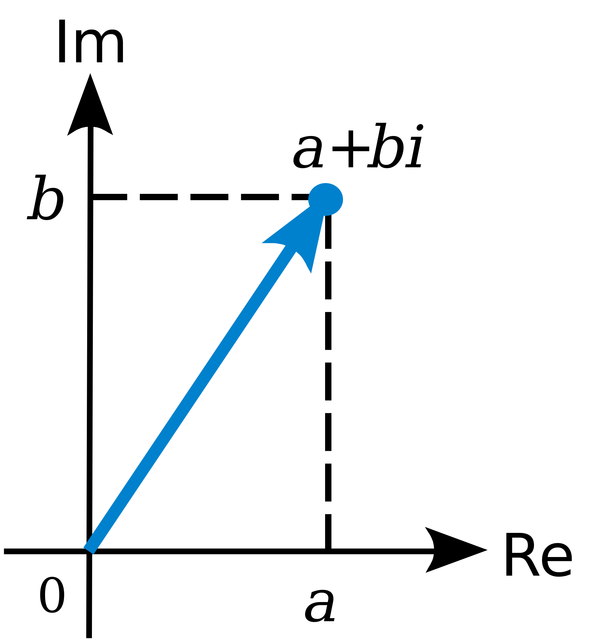
At this point, it’s good to properly define the radian as a unit in quantum mechanics. We often think of a radian as some distance measured along the circumference, because of the way the unit is constructed (see the illustration below) but that’s right and wrong at the same time. In fact, it’s more wrong than right: the radian is an angle that’s defined using the length of the radius of the unit circle but, when everything is said and done, it’s a unit used to measure some angle—not a distance. That should be obvious from the 2π rad = 360 degrees identity. The angle here is the argument of our wavefunction in quantum mechanics, and so that argument combines both time (t) as well as distance (x): θ = kx – ωt = k(x – c∙t). So our angle (the argument of the wavefunction) integrates both dimensions: space as well as time. If you’re not convinced, just do the dimensional analysis of the kx – ωt expression: both the kx and ωt yield a dimensionless number—or… Well… To be precise, I should say: the kx and ωt products both yield an angle expressed in radians. That angle connects the real and imaginary part of the argument of the wavefunction. Hence, it’s a dimensionless number—but that does not imply it is just some meaningless number. It’s not meaningless at all—obviously!

Let me try to present what I wrote above in yet another way. The θ = kx – ωt = (p/ħ)·x − (E/ħ)·t equation suggests a fungibility: the wavefunction itself also expresses itself in time and/or in space, so to speak—just like the quantum of action. Let me be precise: the p·x factor in the (p/ħ)·x term represents momentum (whose dimension is N·s) being expended over a distance, while the E·t factor in the (E/ħ)·t term represents energy (expressed in N·m) being expended over some time. [As for the minus sign in front of the (E/ħ)·t term, that’s got to do with the fact that the arrow of time points in one direction only while, in space, we can go in either direction: forward or backwards.] Hence, the expression for the argument tells us that both are essentially fungible—which suggests they’re aspects of one and the same thing. So that‘s what Minkowski intuition is all about: spacetime is one, and the wavefunction just connects the physical properties of whatever it is that we are observing – an electron, or a photon, or whatever other elementary particle – to it.
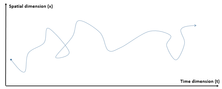
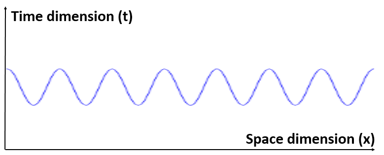
Of course, the corollary to thinking of unified spacetime is thinking of the real and imaginary part of the wavefunction as one—which we’re supposed to do as a complex number is… Well… One complex number. But that’s easier said than actually done, of course. One way of thinking about the connection between the two spacetime ‘dimensions’ – i.e. t and x, with x actually incorporating three spatial dimensions in space in its own right (see how confusing the term ‘dimension’ is?) – and the two ‘dimensions’ of a complex number is going from Cartesian to polar coordinates, and vice versa. You now think of Euler’s formula, of course – if not, you should – but let me insert something more interesting here. 🙂 I took it from Wikipedia. It illustrates how a simple sinusoidal function transforms as we go from Cartesian to polar coordinates.

Interesting, isn’t it? Think of the horizontal and vertical axis in the Cartesian space as representing time and… Well… Space indeed. 🙂 The function connects the space and time dimension and might, for example, represent the trajectory of some object in spacetime. Admittedly, it’s a rather weird trajectory, as the object goes back and forth in some box in space, and accelerates and decelerates all of the time, reversing its direction in the process… But… Well… Isn’t that how we think of a an electron moving in some orbital? 🙂 With that in mind, look at how the same movement in spacetime looks like in polar coordinates. It’s also some movement in a box—but both the ‘horizontal’ and ‘vertical’ axis (think of these axes as the real and imaginary part of a complex number) are now delineating our box. So, whereas our box is a one-dimensional box in spacetime only (our object is constrained in space, but time keeps ticking), it’s a two-dimensional box in our ‘complex’ space. Isn’t it just nice to think about stuff this way?
As far as I am concerned, it triggers the same profound thoughts as that E/p = ω/k relation. The left-hand side is a ratio between energy and momentum. Now, one way to look at energy is that it’s action per time unit. Likewise, momentum is action per distance unit. Of course, ω is expressed as some quantity (expressed in radians, to be precise) per time unit, and k is some quantity (again, expressed in radians) per distance unit. Because this is a physical equation, the dimension of both sides of the equation has to be the same—and, of course, it is the same: the action dimension in the numerator and denominator of the ratio on the left-hand side of the E/p = ω/k equation cancel each other. But… What? Well… Wouldn’t it be nice to think of the dimension of the argument of our wavefunction as being the dimension of action, rather than thinking of it as just some mathematical thing, i.e. an angle. I like to think the argument of our wavefunction is more than just an angle. When everything is said and done, it has to be something physical—if onlyh because the wavefunction describes something physical. But… Well… I need to do some more thinking on this, so I’ll just move on here. Otherwise this post risks becoming a book in its own right. 🙂
Let’s get back to the topic we were discussing here. We were talking about natural units. More in particular, we were wondering: what’s natural? What does it mean?
Back to Planck units
Let’s start with time and distance. We may want to think of lP and tP as the smallest distance and time units possible—so small, in fact, that both distance and time become countable variables at that scale.
Huh? Yes. I am sure you’ve never thought of time and distance as countable variables but I’ll come back to this rather particular interpretation of the Planck length and time unit later. So don’t worry about it now: just make a mental note of it. The thing is: if tP and lP are the smallest time and distance units possible, then the smallest cycle we can possibly imagine will be associated with those two units: we write: ωP = 1/tP and kP = 1/lP. What’s the ‘smallest possible’ cycle? Well… Not sure. You should not think of some oscillation in spacetime as for now. Just think of a cycle. Whatever cycle. So, as for now, the smallest cycle is just the cycle you’d associate with the smallest time and distance units possible—so we cannot write ωP = 2/tP, for example, because that would imply we can imagine a time unit that’s smaller than tP, as we can associate two cycles with tP now.
OK. Next step. We can now define the Planck energy and the Planck momentum using the de Broglie relations:
EP = ħ∙ωP = ħ/tP and pP = ħ∙kP = ħ/lP
You’ll say that I am just repeating myself here, as I’ve given you those two equations already. Well… Yes and no. At this point, you should raise the following question: why are we using the angular frequency (ωP = 2π·fP) and the reduced Planck constant (ħ = h/2π), rather than fP or h?
That’s a great question. In fact, it begs the question: what’s the physical constant really? We have two mathematical constants – ħ and h – but they must represent the same physical reality. So is one of the two constants more real than the other? The answer is unambiguously: yes! The Planck energy is defined as EP = ħ/tP =(h/2π)/tP, so we cannot write this as EP = h/tP. The difference is that 1/2π factor, and it’s quite fundamental, as it implies we’re actually not associating a full cycle with tP and lP but a radian of that cycle only.
Huh? Yes. It’s a rather strange observation, and I must admit I haven’t quite sorted out what this actually means. The fundamental idea remains the same, however: we have a quantum of action, ħ (not h!), that can express itself as energy over the smallest distance unit possible or, alternatively, that expresses itself as momentum over the smallest time unit possible. In the former case, we write it as EP = FP∙lP = ħ/tP. In the latter, we write it as pP = FP∙tP = ħ/lP. Both are aspects of the same reality, though, as our particle moves in space as well as in time, i.e. it moves in spacetime. Hence, one step in space, or in time, corresponds to one radian. Well… Sort of… Not sure how to further explain this. I probably shouldn’t try anyway. 🙂
The more fundamental question is: with what speed is is moving? That question brings us to the next point. The objective is to get some specific value for lP and tP, so how do we do that? How can we determine these two values? Well… That’s another great question. 🙂
The first step is to relate the natural time and distance units to the wave velocity. Now, we do not want to complicate the analysis and so we’re not going to throw in some rest mass or potential energy here. No. We’ll be talking a theoretical zero-mass particle. So we’re not going to consider some electron moving in spacetime, or some other elementary particle. No. We’re going to think about some zero-mass particle here, or a photon. [Note that a photon is not just a zero-mass particle. It’s similar but different: in one of my previous posts, I showed a photon packs more energy, as you get two wavefunctions for the price of one, so to speak. However, don’t worry about the difference here.]
Now, you know that the wave velocity for a zero-mass particle and/or a photon is equal to the speed of light. To be precise, the wave velocity of a photon is the speed of light and, hence, the speed of any zero-mass particle must be the same—as per the definition of mass in Einstein’s special relativity theory. So we write: lP/tP = c ⇔ lP = c∙tP and tP = lP/c. In fact, we also get this from dividing EP by pP, because we know that E/p = c, for any photon (and for any zero-mass particle, really). So we know that EP/pP must also equal c. We can easily double-check that by writing: EP/pP = (ħ/tP)/(ħ/lP) = lP/tP = c. Substitution in ħ = FP∙lP∙tP yields ħ = c∙FP∙tP2 or, alternatively, ħ = FP∙lP2/c. So we can now write FP as a function of lP and/or tP:
FP = ħ∙c/lP2 = ħ/(c∙tP2)
We can quickly double-check this by dividing FP = ħ∙c/lP2 by FP = ħ/(c∙tP2). We get: 1 = c2∙tP2/lP2 ⇔ lP2/tP2 = c2 ⇔ lP/tP = c.
Nice. However, this does not uniquely define FP, lP, and tP. The problem is that we’ve got only two equations (ħ = FP∙lP∙tP and lP/tP = c) for three unknowns (FP, lP, and tP). Can we throw in one or both of the de Broglie equations to get some final answer?
I wish that would help, but it doesn’t—because we get the same ħ = FP∙lP∙tP equation. Indeed, we’re just re-defining the Planck energy (and the Planck momentum) by that EP = ħ/tP (and pP = ħ/lP) equation here, and so that does not give us a value for EP (and pP). So we’re stuck. We need some other formula so we can calculate the third unknown, which is the Planck force unit (FP). What formula could we possibly choose?
Well… We got a relationship by imposing the condition that lP/tP = c, which implies that if we’d measure the velocity of a photon in Planck time and distance units, we’d find that its velocity is one, so c = 1. Can we think of some similar condition involving ħ? The answer is: we can and we can’t. It’s not so simple. Remember we were thinking of the smallest cycle possible? We said it was small because tP and lP were the smallest units we could imagine. But how do we define that? The idea is as follows: the smallest possible cycle will pack the smallest amount of action, i.e. h (or, expressed per radian rather than per cycle, ħ).
Now, we usually think of packing energy, or momentum, instead of packing action, but that’s because… Well… Because we’re not good at thinking the way Minkowski wanted us to think: we’re not good at thinking of some kind of union of space and time. We tend to think of something moving in space, or, alternatively, of something moving in time—rather than something moving in spacetime. In short, we tend to separate dimensions. So that’s why we’d say the smallest possible cycle would pack an amount of energy that’s equal to EP = ħ∙ωP = ħ/tP, or an amount of momentum that’s equal to pP = ħ∙kP = ħ/lP. But both are part and parcel of the same reality, as evidenced by the E = m∙c2 = m∙c∙c = p∙c equality. [This equation only holds for a zero-mass particle (and a photon), of course. It’s a bit more complicated when we’d throw in some rest mass, but we can do that later. Also note I keep repeating my idea of the smallest cycle, but we’re talking radians of a cycle, really.]
So we have that mass-energy equivalence, which is also a mass-momentum equivalence according to that E = m∙c2 = m∙c∙c = p∙c formula. And so now the gravitational force comes into play: there’s a limit to the amount of energy we can pack into a tiny space. Or… Well… Perhaps there’s no limit—but if we pack an awful lot of energy into a really tiny speck of space, then we get a black hole.
However, we’re getting a bit ahead of ourselves here, so let’s first try something else. Let’s throw in the Uncertainty Principle.
The Uncertainty Principle
As mentioned above, we can think of some amount of action expressing itself over some time or, alternatively, over some distance. In the former case, some amount of energy is expended over some time. In the latter case, some momentum is expended over some distance. That’s why the energy and time variables, and the momentum and distance variables, are referred to as complementary. It’s hard to think of both things happening simultaneously (whatever that means in spacetime), but we should try! Let’s now look at the Uncertainty relations once again (I am writing uncertainty with a capital U out of respect—as it’s very fundamental, indeed!):
ΔpΔx ≥ ħ/2 and ΔEΔt ≥ ħ/2.
Note that the ħ/2 factor on the right-hand side quantifies the uncertainty, while the right-hand side of the two equations (ΔpΔx and ΔEΔt) are just an expression of that fundamental uncertainty. In other words, we have two equations (a pair), but there’s only one fundamental uncertainty, and it’s an uncertainty about a movement in spacetime. Hence, that uncertainty expresses itself in both time as well as in space.
Note the use of ħ rather than h, and the fact that the 1/2 factor makes it look like we’re splitting ħ over ΔpΔx and ΔEΔt respectively—which is actually a quite sensible explanation of what this pair of equations actually represent. Indeed, we can add both relations to get the following sum:
ΔpΔx + ΔEΔt ≥ ħ/2 + ħ/2 = ħ
Interesting, isn’t it? It explains that 1/2 factor which troubled us when playing with the de Broglie relations.
Let’s now think about our natural units again—about lP, and tP in particular. As mentioned above, we’ll want to think of them as the smallest distance and time units possible: so small, in fact, that both distance and time become countable variables, so we count x and t as 0, 1, 2, 3 etcetera. We may then imagine that the uncertainty in x and t is of the order of one unit only, so we write Δx = lP and Δt = tP. So we can now re-write the uncertainty relations as:
Hey! Wait a minute! Do we have a solution for the value of lP and tP here? What if we equate the natural energy and momentum units to ΔE and Δp here? Well… Let’s try it. First note that we may think of the uncertainty in t, or in x, as being equal to plus or minus one unit, i.e. ±1. So the uncertainty is two units really. [Frankly, I just want to get rid of that 1/2 factor here.] Hence, we can re-write the ΔpΔx = ΔEΔt = ħ/2 equations as:
- ΔpΔx = pP∙lP = FP∙tP∙lP = ħ
- ΔEΔt = EP∙tP = FP∙lP∙tP = ħ
Hmm… What can we do with this? Nothing much, unfortunately. We’ve got the same problem: we need a value for FP (or for pP, or for EP) to get some specific value for lP and tP, so we’re stuck once again. We have three variables and two equations only, so we have no specific value for either of them. 😦
What to do? Well… I will give you the answer now—the answer you’ve been waiting for, really—but not the technicalities of it. There’s a thing called the Schwarzschild radius, aka as the gravitational radius. Let’s analyze it.
The Schwarzschild radius and the Planck length
The Schwarzschild radius is just the radius of a black hole. Its formal definition is the following: it is the radius of a sphere such that, if all the mass of an object were to be compressed within that sphere, the escape velocity from the surface of the sphere would equal the speed of light (c). The formula for the Schwartzschild radius is the following:
RS = 2m·G/c2
G is the gravitational constant here: G ≈ 6.674×10⁻¹¹ N⋅m2/kg2. [Note that Newton’s F = m·a Law tells us that 1 kg = 1 N·s2/m, as we’ll need to substitute units later.]
But what is the mass (m) in that RS = 2m·G/c2 equation? Using equivalent time and distance units (so c = 1), we wrote the following for a zero-mass particle and for a photon respectively:
- E = m = p = ħ/2 (zero-mass particle)
- E = m = p = ħ (photon)
How can a zero-mass particle, or a photon, have some mass? Well… Because it moves at the speed of light. I’ve talked about that before, so I’ll just refer you to my post on that. Of course, the dimension of the right-hand side of these equations (i.e. ħ/2 or ħ) symbol has to be the same as the dimension on the left-hand side, so the ‘ħ’ in the E = ħ equation (or E = ħ/2 equation) is a different ‘ħ’ in the p = ħ equation (or p = ħ/2 equation). So we must be careful here. Let’s write it all out, so as to remind ourselves of the dimensions involved:
- E [N·m] = ħ [N·m·s/s] = EP = FP∙lP∙tP/tP
- p [N·s] = ħ [N·m·s/m] = pP = FP∙lP∙tP/lP
Now, let’s check this by cheating. I’ll just give you the numerical values—even if we’re not supposed to know them at this point—so you can see I am not writing nonsense here:
- EP = 1.0545718×10⁻³⁴ N·m·s/(5.391×10−44 s) = (1.21×1044 N)·(1.6162×10⁻³⁵ m) = 1.9561×10⁹ N·m
- pP =1.0545718×10⁻³⁴ N·m·s/(1.6162×10−35 m) = (1.21×1044 N)·(5.391×10−44 s) = 6.52485 N·s
You can google the Planck units, and you’ll see I am not taking you for a ride here. 🙂
The associated Planck mass is mP = EP/c2 = 1.9561×10⁹ N·m/(2.998×108 m/s)2 = 2.17651×10⁻⁸ N·s2/m = 2.17651×10⁻⁸ kg. So let’s plug that value into RS = 2m·G/c2 equation. We get:
RS = 2m·G/c2 = [(2.17651×10⁻⁸ kg)·(6.674×10⁻¹¹ N⋅m2/kg2 )/(8.988×1016 m2·s−2)
= 1.6162×10⁻³⁵ kg·N⋅m2·kg−2·m2·s−2 = 1.6162×10⁻³⁵ kg·N⋅m2·kg−2·m2·s−2 = 1.6162×10⁻³⁵ m = lP
Bingo! You can look it up: 1.6162×10⁻³⁵ m is the Planck length indeed, so the Schwarzschild radius is the Planck length. We can now easily calculate the other Planck units:
- tP = lP/c = 1.6162×10⁻³⁵ m/(2.998×108 m/s) = 5.391×10−44 s
- FP = ħ/(tP∙lP)= (1.0545718×10⁻³⁴ N·m·s)/[(1.6162×10−35 m)·(5.391×10−44 s) = 1.21×10−44 N
Bingo again! 🙂
[…] But… Well… Look at this: we’ve been cheating all the way. First, we just gave you that formula for the Schwarzschild radius. It looks like an easy formula but its derivation involves a profound knowledge of general relativity theory. So we’d need to learn about tensors and what have you. The formula is, in effect, a solution to what is known as Einstein’s field equations, and that’s pretty complicated stuff.
However, my crime is much worse than that: I also gave you those numerical values for the Planck energy and momentum, rather than calculating them. I just couldn’t calculate them with the knowledge we have so far. When everything is said and done, we have more than three unknowns. We’ve got five in total, including the Planck charge (qP) and, hence, we need five equations. Again, I’ll just copy them from Wikipedia, because… Well… What we’re discussing here is way beyond the undergraduate physics stuff that we’ve been presenting so far. The equations are the following. Just have a look at them and move on. 🙂

Finally, I should note one more thing: I did not use 2m but m in Schwarzschild’s formula. Why? Well… I have no good answer to that. I did it to ensure I got the result we wanted to get. It’s that 1/2 factor again. In fact, the E = m = p = ħ/2 is the correct formula to use, and all would come out alright if we did that and defined the magnitude of the uncertainty as one unit only, but so we used the E = m = p = ħ formula instead, i.e. the equation that’s associated with a photon. You can re-do the calculations as an exercise: you’ll see it comes out alright.
Just to make things somewhat more real, let me note that the Planck energy is very substantial: 1.9561×10⁹ N·m ≈ 2×10⁹ J is equivalent to the energy that you’d get out of burning 60 liters of gasoline—or the mileage you’d get out of 16 gallons of fuel! In short, it’s huge, and so we’re packing that into a unimaginably small space. To understand how that works, you can think of the E = h∙f ⇔ h = E/f relation once more. The h = E/f ratio implies that energy and frequency are directly proportional to each other, with h the coefficient of proportionality. Shortening the wavelength, amounts to increasing the frequency and, hence, the energy. So, as you think of our cycle becoming smaller and smaller, until it becomes the smallest cycle possible, you should think of the frequency becoming unimaginably large. Indeed, as I explained in one of my other posts on physical constants, we’re talking the the 1043 Hz scale here. However, we can always choose our time unit such that we measure the frequency as one cycle per time unit. Because the energy per cycle remains the same, it means the quantum of action (ħ = FP∙lP∙tP) expresses itself over extremely short time spans, which means the EP = FP∙lP product becomes huge, as we’ve shown above. The rest of the story is the same: gravity comes into play, and so our little blob in spacetime becomes a tiny black hole. Again, we should think of both space and time: they are joined in ‘some kind of union’ here, indeed, as they’re intimately connected through the wavefunction, which travels at the speed of light.
The wavefunction as an oscillation in and of spacetime
OK. Now I am going to present the big idea I started with. Let me first ask you a question: when thinking about the Planck-Einstein relation (I am talking about the E = ħ∙ω relation for a photon here, rather than the equivalent de Broglie equation for a matter-particle), aren’t you struck by the fact that the energy of a photon depends on the frequency of the electromagnetic wave only? I mean… It does not depend on its amplitude. The amplitude is mentioned nowhere. The amplitude is fixed, somehow—or considered to be fixed.
Isn’t that strange? I mean… For any other physical wave, the energy would not only depend on the frequency but also on the amplitude of the wave. For a photon, however, it’s just the frequency that counts. Light of the same frequency but higher intensity (read: more energy) is not a photon with higher amplitude, but just more photons. So it’s the photons that add up somehow, and so that explains the amplitude of the electric and magnetic field vectors (i.e. E and B) and, hence, the intensity of the light. However, every photon considered separately has the same amplitude apparently. We can only increase its energy by increasing the frequency. In short, ω is the only variable here.
Let’s look at that angular frequency once more. As you know, it’s expressed in radians per second but, if you multiply ω by 2π, you get the frequency you’re probably more acquainted with: f = 2πω = f cycles per second. The Planck-Einstein relation is then written as E = h∙f. That’s easy enough. But what if we’d change the time unit here? For example, what if our time unit becomes the time that’s needed for a photon to travel one meter? Let’s examine it.
Let’s denote that time unit by tm, so we write: 1 tm = 1/c s ⇔ tm–1 = c s–1, with c ≈ 3×10⁸. The frequency, as measured using our new time unit, changes, obviously: we have to divide its former value by c now. So, using our little subscript once more, we could write: fm = f/c. [Why? Just add the dimension to make things more explicit: f s–1 = f/c tm–1 = f/c tm–1.] But the energy of the photon should not depend on our time unit, should it?
Don’t worry. It doesn’t: the numerical value of Planck’s constant (h) would also change, as we’d replace the second in its dimension (N∙m∙s) by c times our new time unit tm. However, Planck’s constant remains what it is: some physical constant. It does not depend on our measurement units: we can use the SI units, or the Planck units (FP, lP, and tP), or whatever unit you can think of. It doesn’t matter: h (or ħ = h/2π) is what is—it’s the quantum of action, and so that’s a physical constant (as opposed to a mathematical constant) that’s associated with one cycle.
Now, I said we do not associate the wavefunction of a photon with an amplitude, but we do associate it with a wavelength. We do so using the standard formula for the velocity of a wave: c = f∙λ ⇔ λ = c/f. We can also write this using the angular frequency and the wavenumber: c = ω/k, with k = 2π/λ. We can double-check this, because we know that, for a photon, the following relation holds: E/p = c. Hence, using the E = ħ∙ω and p = ħ∙k relations, we get: (ħ∙ω)/(ħ∙k) = ω/k = c. So we have options here: h can express itself over a really long wavelength, or it can do so over an extremely short wavelength. We re-write p = ħ∙k as p = E/c = ħ∙2π/λ = h/λ ⇔ E = h∙c/λ ⇔ h∙c = E∙λ. We know this relationship: the energy and the wavelength of a photon (or an electromagnetic wave) are inversely proportional to each other.
Once again, we may want to think of the shortest wavelength possible. As λ gets a zillion times smaller, E gets a zillion times bigger. Is there a limit? There is. As I mentioned above, the gravitational force comes into play here: there’s a limit to the amount of energy we can pack into a tiny space. If we pack an awful lot of energy into a really tiny speck of space, then we get a black hole. In practical terms, that implies our photon can’t travel, as it can’t escape from the black hole it creates. That’s what that calculation of the Schwarzschild radius was all about.
We can—in fact, we should—now apply the same reasoning to the matter-wave. Instead of a photon, we should try to think of a zero-mass matter-particle. You’ll say: that’s a contradiction. Matter-particles – as opposed to force-carrying particles, like photons (or bosons in general) – must have some rest mass, so they can’t be massless. Well… Yes. You’re right. But we can throw the rest mass in later. I first want to focus on the abstract principles, i.e. the propagation mechanism of the matter-wave.
Using natural units, we know our particle will move in spacetime with velocity Δx/Δt = 1/1 = 1. Of course, it has to have some energy to move, or some momentum. We also showed that, if it’s massless, and the elementary wavefunction is ei[(p/ħ)x – (E/ħ)t), then we know the energy, and the momentum, has to be equal to ħ/2. Where does it get that energy, or momentum? Not sure. I like to think it borrows it from spacetime, as it breaks some potential barrier between those two points, and then it gives it back. Or, if it’s at point x = t = 0, then perhaps it gets it from some other massless particle moving from x = t = −1. In both cases, we’d like to think our particle keeps moving. So if the first description (borrowing) is correct, it needs to keep borrowing and returning energy in some kind of interaction with spacetime itself. If it’s the second description, it’s more like spacetime bumping itself forward.
In both cases, however, we’re actually trying to visualize (or should I say: imagine?) some oscillation of spacetime itself, as opposed to an oscillation in spacetime.
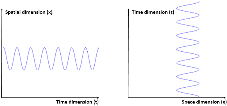
Huh? Yes. The idea is the following here: we like to think of the wavefunction as the dependent variable: both its real as well as its imaginary part are a function of x and t, indeed. But what if we’d think of x and t as dependent variables? In that case, the real and imaginary part of the wavefunction would be the independent variables. It’s just a matter of perspective. We sort of mirror our function: we switch its domain for its range, and its range for its domain, as shown below. It all makes sense, doesn’t it? Space and time appear as separate dimensions to us, but they’re intimately connected through c, ħ and the other fundamental physical constants. Likewise, the real and imaginary part of the wavefunction appear as separate dimensions, but they’re intimately connected through π and Euler’s number, i.e. through mathematical constants. That cannot be a coincidence: the mathematical and physical ‘space’ reflect each other through the wavefunction, just like the domain and range of a function reflect each other through that function. So physics and math must meet in some kind of union—at least in our mind, they do!

So, yes, we can—and probably should—be looking at the wavefunction as an oscillation of spacetime, rather than as an oscillation in spacetime only. As mentioned in my introduction, I’ll need to study general relativity theory—and very much in depth—to convincingly prove that point, but I am sure it can be done.
You’ll probably think I am arrogant when saying that—and I probably am—but then I am very much emboldened by the fact some nuclear scientist told me a photon doesn’t have any wavefunction: it’s just those E and B vectors, he told me—and then I found out he was dead wrong, as I showed in my previous post! So I’d rather think more independently now. I’ll keep you guys posted on progress—but it will probably take a while to figure it all out. In the meanwhile, please do let me know your ideas on this. 🙂
Let me wrap up this little excursion with two small notes:
- We have this E/c = p relation. The mass-energy equivalence relation implies momentum must also have an equivalent mass. If E = m∙c2, then p = m∙c ⇔ m = p/c. It’s obvious, but I just thought it would be useful to highlight this.
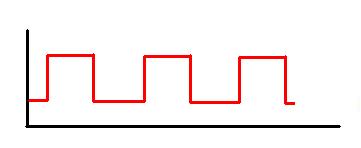
- When we studied the ammonia molecule as a two-state system, our space was not a continuum: we allowed just two positions—two points in space, which we defined with respect to the system. So x was a discrete variable. We assumed time to be continuous, however, and so we got those nice sinusoids as a solution to our set of Hamiltonian equations. However, if we look at space as being discrete, or countable, we should probably think of time as being countable as well. So we should, perhaps, think of a particle being at point x = t = 0 first, and, then, being at point x = t = 1. Instead of the nice sinusoids, we get some boxcar function, as illustrated below, but probably varying between 0 and 1—or whatever other normalized values. You get the idea, I hope. 🙂

Post Scriptum on the Principle of Least Action: As noted above, the Principle of Least Action is not very intuitive, even if Feynman’s exposé of it is not as impregnable as it may look at first. To put it simply, the Principle of Least Action says that the average kinetic energy less the average potential energy is as little as possible for the path of an object going from one point to another. So we have a path or line integral here. In a gravitation field, that integral is the following:

The integral is not all that important. Just note its dimension is the dimension of action indeed, as we multiply energy (the integrand) with time (dt). We can use the Principle of Least Action to re-state Newton’s Law, or whatever other classical law. Among other things, we’ll find that, in the absence of any potential, the trajectory of a particle will just be some straight line.
In quantum mechanics, however, we have uncertainty, as expressed in the ΔpΔx ≥ ħ/2 and ΔEΔt ≥ ħ/2 relations. Now, that uncertainty may express itself in time, or in distance, or in both. That’s where things become tricky. 🙂 I’ve written on this before, but let me copy Feynman himself here, with a more exact explanation of what’s happening (just click on the text to enlarge):
The ‘student’ he speaks of above, is himself, of course. 🙂
Too complicated? Well… Never mind. I’ll come back to it later. 🙂
Some content on this page was disabled on June 16, 2020 as a result of a DMCA takedown notice from The California Institute of Technology. You can learn more about the DMCA here:
https://wordpress.com/support/copyright-and-the-dmca/
Some content on this page was disabled on June 17, 2020 as a result of a DMCA takedown notice from Michael A. Gottlieb, Rudolf Pfeiffer, and The California Institute of Technology. You can learn more about the DMCA here:
https://wordpress.com/support/copyright-and-the-dmca/


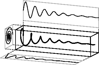
 As Feynman writes, all of the wave functions approach zero rapidly for large r (also, confusingly, denoted as ρ) after oscillating a few times, with the number of ‘bumps’ equal to n. Of course, you should note that you should put the time factor back in in order to correctly interpret these functions. Indeed, remember how we separated them when we wrote:
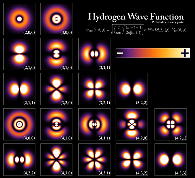
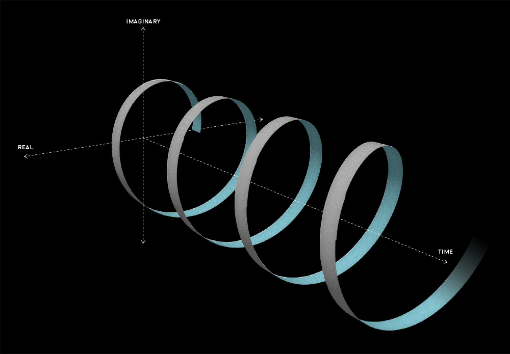
 Now think of wrapping that around some circle. We’d get something like below. [Don’t worry about the precise shape of the graph, as I made up a new one. Note the remark on the need to have a well-behaved function applies here too!]
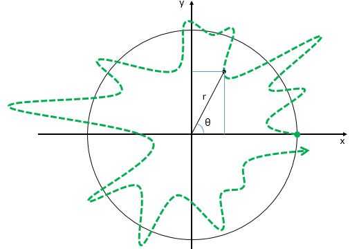 Neat, you’ll say, but so what? All we’ve done so far is show that we can represent some itinerary in spacetime in two different ways. In the first representation, we measure time along some linear axis, while, in the second representation, time becomes some angle—an angle that increases, counter-clockwise. To put it differently: time becomes an angular velocity.
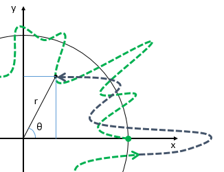


