Field energy and field momentum

This post goes to the heart of the E = mc², equation. It’s kinda funny, because Feynman just compresses all of it in a sub-section of his Lectures. However, as far as I am concerned, I feel it’s a very crucial section. Pivotal, I’d say, which would fit with its place in all of the 115 Lectures that make up the three volumes, which is sort of mid-way, which is where we are here. So let’s get go for it. 🙂

Let’s first recall what we wrote about the Poynting vector S, which we calculate from the magnetic and electric field vectors E and B by taking their cross-product:

This vector represents the energy flow, per unit area and per unit time, in electrodynamical situations. If E and/or B are zero (which is the case in electrostatics, for example, because we don’t have magnetic fields in electrostatics), then S is zero too, so there is no energy flow then. That makes sense, because we have no moving charges, so where would the energy go to?

I also made it clear we should think of S as something physical, by comparing it to the heat flow vector h, which we presented when discussing vector analysis and vector operators. The heat flow out of a surface element da is the area times the component of h perpendicular to da, so that’s (h•n)·da = h_n·da. Likewise, we can write (S•n)·da = S_n·da. The units of S and h are also the same: joule per second and per square meter or, using the definition of the watt (1 W = 1 J/s), in watt per square meter. In fact, if you google a bit, you’ll find that both h and S are referred to as a flux density:

The heat flow vector h is the heat flux density vector, from which we get the heat flux through an area through the (h•n)·da = h_n·da product.
The energy flow S is the energy flux density vector, from which we get the energy flux through the (S•n)·da = S_n·da product.

So that should be enough as an introduction to what I want to talk about here. Let’s first look at the energy conservation principle once again.

Local energy conservation

In a way, you can look at my previous post as being all about the equation below, which we referred to as the ‘local’ energy conservation law:

Of course, it is not the complete energy conservation law. The local energy is not only in the field. We’ve got matter as well, and so that’s what I want to discuss here: we want to look at the energy in the field as well as the energy that’s in the matter. Indeed, field energy is conserved, and then it isn’t: if the field is doing work on matter, or matter is doing work on the field, then… Well… Energy goes from one to the other, i.e. from the field to the matter or from the matter to the field. So we need to include matter in our analysis, which we didn’t do in our last post. Feynman gives the following simple example: we’re in a dark room, and suddenly someone turns on the light switch. So now the room is full of field energy—and, yes, I just mean it’s not dark anymore. :-). So that means some matter out there must have radiated its energy out and, in the process, it must have lost the equivalent mass of that energy. So, yes, we had matter losing energy and, hence, losing mass.

Now, we know that energy and momentum are related. Respecting and incorporating relativity theory, we’ve got two equivalent formulas for it:

E²− p²c² = m₀²c⁴
pc = E·(v/c) ⇔ p = v·E/c²= m·v

The E = mc² and m = ·m₀·(1−v²/c²)^−1/2 formulas connect both expressions. So we can look at it in either of two ways. We could use the energy conservation law, but Feynman prefers the conservation of momentum approach, so let’s see where he takes us. If the field has some energy (and, hence, some equivalent mass) per unit volume, and if there’s some flow, so if there’s some velocity (which there is: that’s what our previous post was all about), then it will have a certain momentum per unit volume. [Remember: momentum is mass times velocity.] That momentum will have a direction, so it’s a vector, just like p = mv. We’ll write it as g, so we define g as:

g is the momentum of the field per unit volume.

What units would we express it in? We’ve got a bit of choice here. For example, because we’re relating everything to energy here, we may want to convert our kilogram into eV/c²or J/c²units, using the mass-energy equivalence relation E = mc². Hmm… Let’s first keep the kg as a measure of inertia though. So we write: [g] = [m]·[v]/m³= (kg·m/s)/m³. Hmm… That doesn’t show it’s energy, so let’s replace the kg with a unit that’s got newton and meter in it, cf. the F = ma law. So we write: [g] = (kg·m/s)/m³= (kg/s)/m²= [(N·s²/m)/s]/m²= N·s/m³. Well… OK. The newton·second is the unit of momentum indeed, and we can re-write it including the joule (1 J = 1 N·m), so then we get [g] = (J·s/m⁴), so what’s that? Well… Nothing much. However, I do note it happens to be the dimension of S/c², so that’s [S/c²] = [J/(s·m²)]·(s²/m²) = (J·s/m⁴). 🙂 Let’s continue the discussion.

Now, momentum is conserved, and each component of it is conserved. So let’s look at the x-direction. We should have something like:

If you look at this carefully, you’ll probably say: “OK. I understood the thing with the dark room and light switch. Mass got converted into field energy, but what’s that second term of the left?”

Good. Smart. Right remark. Perfect. […] Let me try to answer the question. While all of the quantities above are expressed per unit volume, we’re actually looking at the same infinitesimal volume element here, so the example of the light switch is actually an example of a ‘momentum outflow’, so it’s actually an example of that second term of the left-hand side of the equation above kicking in! 🙂

Indeed, the first term just sort of reiterates the mass-energy equivalence: the energy that’s in the matter can become field energy, so to speak, in our infinitesimal volume element itself, and vice versa. But if it doesn’t, then it should get out and, hence, become ‘momentum outflow’. Does that make sense? No?

Hmm… What to say? You’ll need to look at that equation a couple of times more, I guess. But I need to move on, unfortunately. [Don’t get put off when I say things like this: I am basically talking to myself, so it means I’ll need to re-visit this myself. :-/]

Let’s look at all of the three terms:

The left-hand side (i.e. the time rate-of-change of the momentum of matter) is easy. It’s just the force on it, which we know is equal to F = $q (E + v \times B). Do we know that? OK\dots I’ll admit it. Sometimes it’s easy to forget where we are in an analysis like this, but so we’re looking at the electromagnetic force here. 🙂 As we’re talking infinitesimals here and, therefore, charge density rather than discrete charges, we should re-write this as the force per unit volume which is$ $ρ E + j \times B . [This is an interesting formula which I didn’t use before, so you should double-check it. :-)]$
The first term on the right-hand side should be equally obvious, or… Well… Perhaps somewhat less so. But with all my rambling on the Uncertainty Principle and/or the wave-particle duality, it should make sense. If we scrap the second term on the right-hand side, we basically have an equation that is equivalent to the E = mc² equation. No? Sorry. Just look at it, again and again. You’ll end up understanding it. 🙂
So it’s that second term on the right-hand side. What the hell does that say? Well… I could say: it’s the local energy or momentum conservation law. If the energy or momentum doesn’t stay in, it has to go out. 🙂 But that’s not very satisfactory as an answer, of course. However, please just go along with this ‘temporary’ answer for a while.

So what is that second term on the right-hand side? As we wrote it, it’s an x-component – or, let’s put it differently, it is or was part of the x-component of the momentum density – but, frankly, we should probably allow it to go out in any direction really, as the only constraint on the left-hand side is a per second rate of change of something. Hence, Feynman suggest to equate it to something like this:

What a, b and c? The components of some vector? Not sure. We’re stuck. This piece really requires very advanced math. In fact, as far as I know, this is the only time where Feynman says: “Sorry. This is too advanced. I’ll just give you the equation. Sorry.” So that’s what he does. He explains the philosophy of the argument, which is the following:

On the left-hand side, we’ve got the time rate-of-change of momentum, so that obeys the F = dp/dt = d(mv)/dt law, with the force F, $per unit volume, being equal to F (unit volume) =$ $ρ E + j \times B .$
$On the right-hand side, we’ve got something that can be written as:$

So we’d need to find a way to $ρ E + j \times B$ in terms of $E$ and $B only -$ eliminating $ρ$ and $j$ by using Maxwell’s equations or whatever other trick – and then juggle terms and make substitutions to get it into a form that looks like the formula above, i.e. the right-hand side of that equation. But so Feynman doesn’t show us how it’s being done. He just mentions some theorem in physics, which says that the energy that’s flowing through a unit area per unit time divided by c² – so that’s E/c²per unit area and per unit time – must be equal to the momentum per unit volume in the space, so we write:

g = S/c²

He illustrates the general theorem that’s used to get the equation above by giving two examples:

OK. Two good examples. However, it’s still frustrating to not see how we get the g = S/c² in the specific context of the electromagnetic force, so let’s do a dimensional analysis at least. In my previous post, I showed that the dimension of S must be J/(m²·s), so [S/c²] = [J/(m²·s)]/(m²/s²) = [N·m/(m²·s)]·(s²/m²) = [N·s/m³]. Now, we know that the unit of mass is 1 kg = N/(m/s²). That’s just the force law: a force of 1 newton will give a mass of 1 kg an acceleration of 1 m/s per second, so 1 N = 1 kg·(m/s²). So the [N·s/m³] dimension is equal to [kg·(m/s²)·s/m³] = [(kg·(m/s)/m³] = [(kg·(m/s)]/m³ $, which is the dimension of momentum (p = m v) per unit volume, indeed. So, yes, the dimensional analysis works out, and it’s also in line with the p = v\cdot E / c 2$ $= m\cdot v equation, but\dots Oh\dots We did a dimensional analysis already, where we also showed that [g] = [S / c 2] = (J\cdots/m 4). Well\dots In any case\dots It’s a bit frustrating to not see the detail here, but let us note the the Grand Result once again:$

The Poynting vector S gives us the energy flow as well as the $momentum density$ $g$ = S/c².

But what does it all mean, really? Let’s go through Einstein’s illustration of the principle. That will help us a lot. Before we do, however, I’d like to note something. I’ve always wondered a bit about that dichotomy between energy and momentum. Energy is force times distance: 1 joule is 1 newton × 1 meter indeed (1 J = 1 N·m). Momentum is force times time, as we can express it in N·s. Planck’s constant h combines all three in the dimension of action, which is force times distance times time: h ≈ 6.6×10⁻³⁴ N·m·s, indeed. I like that unity. In this regard, you should, perhaps, quickly review that post in which I explain that h is the energy per cycle, i.e. per wavelength or per period, of a photon, regardless of its wavelength. So it’s really something very fundamental.

We’ve got something similar here: energy and momentum coming together, and being shown as one aspect of the same thing: some oscillation. Indeed, just see what happens with the dimensions when we ‘distribute’ the 1/c²factor on the right-hand side over the two sides, so we write: $c$ $\cdot$ $g$ = S/c and work out the dimensions:

$[$ $c$ $\cdot$ $g$ $]$ = (m/s)·(N·s)/m³= N/m²= J/m³.
[S/c] = (s/m)·(N·m)/(s·m²) = N/m²= J/m³.

Isn’t that nice? Both sides of the equation now have a dimension like ‘the force per unit area’, or ‘the energy per unit volume’. To get that, we just re-scaled g and S, by c and 1/c respectively. As far as I am concerned, this shows an underlying unity we probably tend to mask with our ‘related but different’ energy and momentum concepts. It’s like E and B: I just love it we can write them together in our Poynting formula S = ε₀c²E×B. In fact, let me show something else here, which you should think about. You know that c²= 1/(ε₀μ₀), so we can write S also as S = E×B/μ₀. That’s nice, but what’s nice too is the following:

S/c = $c$ $\cdot$ $g$ = ε₀cE×B = E×B/μ₀c
S/g = c²= 1/(ε₀μ₀)

So, once again, Feynman may feel the Poynting vector is sort of counter-intuitive when analyzing specific situations but, as far as I am concerned, I feel the Poyning vector makes things actually easier to understand. Instead of two E and B vectors, and two concepts to deal with ‘energy’ (i.e. energy and momentum), we’re sort of unifying things here. In that regard – i.e in regard of feeling we’re talking the same thing really – I’d really highlight the S/g = c²= 1/(ε₀μ₀) equation. Indeed, the universal constant c acts just like the fine-structure constant here: it links everything to everything. 🙂

And, yes, it’s also about time we introduce the so-called principle of least action to explain things, because action, as a concept, combines force, distance and time indeed, so it’s a bit more promising than just energy, of just momentum. Having said that, you’ll see in the next section that it’s sometimes quite useful to have the choice between one formula or the other. But… Well… Enough talk. Let’s look at Einstein’s car.

Einstein’s car

Einstein’s car is a wonderful device: it rolls without any friction and it moves with a little flashlight. That’s all it needs. It’s pictured below. 🙂 So the situation is the following: the flashlight shoots some light out from one side, which is then stopped at the opposite end of the car. When the light is emitted, there must be some recoil. In fact, we know it’s going to be equal to 1/c times the energy because all we need to do is apply the pc = E·(v/c) formula for v = c, so we know that p = E/c. Of course, this momentum now needs to move Einstein’s car. It’s frictionless, so it should work, but still… The car has some mass M, and so that will determine its recoil velocity: v = p/M. We just apply the general p = mv formula here, and v is not equal to c here, of course! Of course, then the light hits the opposite end of the car and delivers the same momentum, so that stops the car again. However, it did move over some distance x = vt. So we could flash our light again and get to wherever we want to get. [Never mind the infinite accelerations involved!] So… Well… Great! Yes, but Einstein didn’t like this car when he first saw it. In fact, he still doesn’t like it, because he knows it won’t take you very far. 🙂

The problem is that we seem to be moving the center of gravity of this car by fooling around on the inside only. Einstein doesn’t like that. He thinks it’s impossible. And he’s right of course. The thing is: the center of gravity did not change. What happened here is that we’ve got some blob of energy, and so that blob has some equivalent mass (which we’ll denote by U/c²), and so that equivalent mass moved all the way from one side to the other, i.e. over the length of the car, which we denote by L. In fact, it’s stuff like this that inspired the whole theory of the field energy and field momentum, and how it interacts with matter.

What happens here is like switching the light on in the dark room: we’ve got matter doing work on the field, and so matter loses mass, and the field gains it, through its momentum and/or energy. To calculate how much, we could integrate S/c or $c$ $\cdot$ $g$ over the volume of our blob, and we’d get something in joule indeed, but there’s a simpler way here. The momentum conservation says that the momentum of our car and the momentum of our blob must be equal, so if T is the time that was needed for our blob to go to the other side – and so that’s, of course, also the time during which our car was rolling – then M·v = M·x/T must be equal to (U/c²)·c = (U/c²)·L/T. The 1/T factor on both sides cancel, so we write: M·x = (U/c²)·L. Now, what is x? Yes. In case you were wondering, that’s what we’re looking for here. 🙂 Here it is:

x = vT = vL/c = (p/M)·(L/c) = [U/c)/M]·(L/c) = (U/c²)·(L/M)

So what’s next? Well… Now we need to show that the center-of-mass actually did not move with this ‘transfer’ of the blob. I’ll leave the math to you here: it should all work out. And you can also think through the obvious questions:

Where is the energy and, hence, the mass of our blob after it stops the car? Hint: think about excited atoms and imagine they might radiate some light back. 🙂
As the car did move a little bit, we should be able to move it further and further away from its center of gravity, until the center of gravity is no longer in the car. Hint: think about batteries and energy levels going down while shooting light out. It just won’t happen. 🙂

Now, what about a blob of light going from the top to the bottom of the car? Well… That involves the conservation of angular momentum: we’ll have more mass on the bottom, but on a shorter lever-arm, so angular momentum is being conserved. It’s a very good question though, and it led Einstein to combine the center-of-gravity theorem with the angular momentum conservation theorem to explain stuff like this.

It’s all fascinating, and one can think of a great many paradoxes that, at first, seem to contradict the Grand Principles we used here, which means that they would contradict all that we have learned so far. However, a careful analysis of those paradox reveals that they are paradoxes indeed: propositions which sound true but are, in the end, self-contradictory. In fact, when explaining electromagnetism over his various Lectures, Feynman tasks his readers with a rather formidable paradox when discussing the laws of induction, he solves it here, ten chapters later, after describing what we described above. You can busy yourself with it but… Well… I guess you’ve got something better to do. If so, just take away the key lesson: there’s momentum in the field, and it’s also possible to build up angular momentum in a magnetic field and, if you switch it off, the angular momentum will be given back, somehow, as it’s stored energy.

That’s also why the seemingly irrelevant circulation of S we discussed in my previous post, where we had a charge next to an ordinary magnet, and where we found that there was energy circulating around, is not so queer. The energy is there, in the circulating field, and it’s real. As real as can be. 🙂

The energy of fields and the Poynting vector

For some reason, I always thought that Poynting was a Russian physicist, like Minkowski. He wasn’t. I just looked it up. Poynting was an Englishman, born near Manchester, and he teached in Birmingham. I should have known. Poynting is a very English name, isn’t it? My confusion probably stems from the fact that it was some Russian physicist, Nikolay Umov, who first proposed the basic concepts we are going to discuss here, i.e. the speed and direction of energy itself, or its movement. And as I am double-checking, I just learned that Hermann Minkowski is generally considered to be German-Jewish, not Russian. Makes sense. With Einstein and all that. His personal life story is actually quite interesting. You should check it out. 🙂

Let’s go for it. We’ve done a few posts on the energy in the fields already, but all in the contexts of electrostatics. Let me first walk you through the ideas we presented there.

The basic concepts: force, work, energy and potential

1. A charge q causes an electric field E, and E‘s magnitude E is a simple function of the charge (q) and its distance (r) from the point that we’re looking at, which we usually write as P = (x, y, z). Of course, the origin of our reference frame here is q. The formula is the simple inverse-square law that you (should) know: E ∼ q/r², and the proportionality constant is just Coulomb’s constant, which I think you wrote as k_e in your high-school days and which, as you know, is there so as to make sure the units come out alright. So we could just write E = k_e·q/r². However, just to make sure it does not look like a piece of cake 🙂 physicists write the proportionality constant as 1/4πε₀, so we get:

Now, the field is the force on any unit charge (+1) we’d bring to P. This led us to think of energy, potential energy, because… Well… You know: energy is measured by work, so that’s some force acting over some distance. The potential energy of a charge increases if we move it against the field, so we wrote:

Well… We actually gave the formula below in that post, so that’s the work done per unit charge. To interpret it, you just need to remember that F = qE, which is equivalent to saying that E is the force per unit charge.

As for the F•ds or E•ds product in the integrals, that’s a vector dot product, which we need because it’s only the tangential component of the force that’s doing work, as evidenced by the formula F•ds = |F|·|ds|·cosθ = F_t·ds, and as depicted below.

Now, this allowed us to describe the field in terms of the (electric) potential Φ and the potential differences between two points, like the points a and b in the integral above. We have to chose some reference point, of course, some P₀ defining zero potential, which is usually infinitely far away. So we wrote our formula for the work that’s being done on a unit charge, i.e. W(unit) as:

2. The world is full of charges, of course, and so we need to add all of their fields. But so now you need a bit of imagination. Let’s reconstruct the world by moving all charges out, and then we bring them back one by one. So we take q₁ now, and we bring it back into the now-empty world. Now that does not require any energy, because there’s no field to start with. However, when we take our second charge q₂, we will be doing work as we move it against the field or, if it’s an opposite charge, we’ll be taking energy out of the field. Huh? Yes. Think about it. All is symmetric. Just to make sure you’re comfortable with every step we take, let me jot down the formula for the force that’s involved. It’s just the Coulomb force of course:

F₁is the force on charge q₁, and F₂is the force on charge q₂. Now, q₁and q₂. may attract or repel each other but the forces will always be equal and opposite. The e₁₂ vector makes sure the directions and signs come out alright, as it’s the unit vector from q₂to q₁(not from q₁to q₂, as you might expect when looking at the order of the indices). So we would need to integrate this for r going from infinity to… Well… The distance between q₁and q₂ – wherever they end up as we put them back into the world – so that’s what’s denoted by r₁₂. Now I hate integrals too, but this is an easy one. Just note that ∫ r⁻²dr = 1/r and you’ll be able to figure out that what I’ll write now makes sense (if not, I’ll do a similar integral in a moment): the work done in bringing two charges together from a large distance (infinity) is equal to:

So now we should bring in q₃and then q₄, of course. That’s easy enough. Bringing the first two charges into that world we had emptied took a lot of time, but now we can automate processes. Trust me: we’ll be done in no time. 🙂 We just need to sum over all of the pairs of charges q_i and q_j. So we write the total electrostatic energy U as the sum of the energies of all possible pairs of charges:

Huh? Can we do that? I mean… Every new charge that we’re bringing in here changes the field, doesn’t it? It does. But it’s the magic of the superposition principle at work here. Our third charge q₃is associated with two pairs in this formula. Think of it: we’ve got the q₁q₃and the q₂q₃combination, indeed. Likewise, our fourh charge q₄is to be paired up with three charges now: q₁, q₁ and q₃. This formula takes care of it, and the ‘all pairs’ mention under the summation sign (Σ) reminds us we should watch we don’t double-count pairs: the q₁q₃and q₃q₁combination, for example, count for one pair only, obviously. So, yes, we write ‘all pairs’ instead of the usual i, j subscripts. But then, yes, this formula takes care of it. We’re done!

Well… Not really, of course. We’ve still got some way to go before I can introduce the Poynting vector. 🙂 However, to make sure you ‘get’ the energy formula above, let me insert an extremely simple diagram so you’ve got a bit of a visual of what we’re talking about.

3. Now, let’s take a step back. We just calculated the (potential) energy of the world (U), which is great. But perhaps we should also be interested in the world’s potential Φ, rather than its potential energy U. Why? Well, we’ll want to know what happens when we bring yet another charge in—from outer space or so. 🙂 And so then it’s easier to know the world’s potential, rather than its energy, because we can calculate the field from it using the E = −∇Φ formula. So let’s de- and re-construct the world once again 🙂 but now we’ll look at what happens with the field and the potential.

We know our first charge created a field with a field strength we calculated as:

So, when bringing in our second charge, we can use our Φ(P) integral to calculate the potential:

[Let me make a note here, just for the record. You probably think I am being pretty childish when talking about my re-construction of the world in terms of bringing all charges out and then back in again but, believe me, there will be a lot of confusion when we’ll start talking about the energy of one charge, and that confusion can be avoided, to a large extent, when you realize that the idea (I mean the concept itself, really—not its formula) of a potential involves two charges really. Just remember: it’s the first charge that causes the field (and, of course, any charge causes a field), but calculating a potential only makes sense when we’re talking some other charge. Just make a mental note of it. You’ll be grateful to me later.]

Let’s now combine the integral and the formula for E above. Because you hate integrals as much as I do, I’ll spell it out: the antiderivative of the Φ(P) integral is ∫ q/(4πε₀r²)·dr. Now, let’s bring q/4πε₀out for a while so we can focus on solving ∫(1/r²)dr. Now, ∫(1/r²)dr is equal to –1/r + k, and so the whole antiderivative is –q/4πε₀r + k. Now, we integrate from r = ∞ to r, and so the definite integral is [–q/(4πε₀)]·[1/∞ − 1/r] = [–q/(4πε₀)]·[0 − 1/r] = q/(4πε₀r). Let me present this somewhat nicer:

You’ll say: so what? Well… We’re done! The only thing we need to do now is add up the potentials of all of the charges in the world. So the formula for the potential Φ at a point which we’ll simply refer to as point 1, is:

Note that our index j starts at 2, otherwise it doesn’t make sense: we’d have a division by zero for the q₁/r₁₁ term. Again, it’s an obvious remark, but not thinking about it can cause a lot of confusion down the line.

4. Now, I am very sorry but I have to inform you that we’ll be talking charge densities and all that shortly, rather than discrete charges, so I have to give you the continuum version of this formula, i.e. the formula we’ll use when we’ve got charge densities rather than individual charges. That sum above then becomes an infinite sum (i.e. an integral), and q_j becomes a variable which we write as ρ(2). [That’s totally in line with our index j starts at 2, rather than from 1.] We get:

Just look at this integral, and try to understand it: we’re integrating over all of space – so we’re integrating the whole world, really 🙂 – and the ρ(2)·dV₂product in the integral is just the charge of an infinitesimally small volume of our world. So the whole integral is just the (infinite) sum of the contributions to the potential (at point 1) of all (infinitesimally small) charges that are around indeed. Now, there’s something funny here. It’s just a mathematical thing: we don’t need to worry about double-counting here. Why? We’re not having products of volumes here. Just make a mental note of it because it will be different in a moment.

Now we’re going to look at the continuum version for our energy formula indeed. Which energy formula? That electrostatic energy formula, which said that the total electrostatic energy U as the sum of the energies of all possible pairs of charges:

Its continuum version is the following monster:

Hmm… What kind of integral is that? We’ve got two variables here: dV₂ and dV₁. Yes. And we’ve also got a 1/2 factor now, because we do not want to double-count and, unfortunately, there is no convenient way of writing an integral like this that keeps track of the pairs. It’s a so-called double integral, but I’ll let you look up the math yourself. In any case, we can simplify this integral so you don’t need to worry about it too much. How do we simplify it? Well… Just look at that integral we got for Φ(1): we calculated the potential at point 1 by integrating the ρ(2)·dV₂product over all of space, so the integral above can be written as:

But so this integral integrates the ρ(1)·Φ(1)·dV₁product over all of space, so that’s over all points in space. So we can just drop the index and write the whole thing as the integral of ρ·Φ·dV over all of space:

5. It’s time for the hat-trick now. The equation above is mathematically equivalent to the following equation:

Huh? Yes. Let me make two remarks here. First on the math, the E = −∇Φ formula allows you to the integrand of the integral above as E•E = (−∇Φ)•(−∇Φ) = (∇Φ)•(∇Φ). And then you may or may not remember that, when substituting E = −∇Φ in Maxwell’s first equation (∇•E = ρ/ε₀), we got the following equality: ρ = ε₀·∇•(∇Φ) = ε₀·∇²Φ, so we can write ρΦ as ε₀·Φ·∇²Φ. However, that still doesn’t show the two integrals are the same thing. The proof is actually rather involved, and so I’ll refer to that post I referred to, so you can check the proof there.

The second remark is much more fundamental. The two integrals are mathematically equivalent, but are they also physically? What do I mean with that? Well… Look at it. The second integral implies that we can look at (ε₀/2)·E•E = ε₀E²/2 as an energy density, which we’ll denote by u, so we write:

Just to make sure you ‘get’ what we’re talking about here: u is the energy density in the little cube dV in the rather simplistic (and, therefore, extremely useful) illustration below (which, just like most of what I write above, I got from Feynman).

Now the question: what is the reality of that formula? Indeed, what we did when calculating U amounted to calculating the Universe with some number U – and that’s kinda nice, of course! – but then what? Is u = ε₀E²/2 anything real? Well… That’s what this post is about. So we’re finished with the introduction now. 🙂

Energy density and energy flow in electrodynamics

Before giving you any more formulas, let me answer the question: there is no doubt, in the classical theory of electromagnetism at least, that the energy density u is something very real. It has to be because of the charge conservation law. Charges cannot just disappear in space, to then re-appear somewhere else. The charge conservation law is written as ∇•j = −∂ρ/∂t, and that makes it clear it’s a local conservation law. Therefore, charges can only disappear and re-appear through some current. We write dQ₁/dt = ∫ (j•n)·da = −dQ₂/dt, and here’s the simple illustration that comes with it:

So we do not allow for any ‘non-local’ interactions here! Therefore, we say that, if energy goes away from a region, it’s because it flows away through the boundaries of that region. So that’s what the Poynting formulas are all about, and so I want to be clear on that from the outset.

Now, to get going with the discussion, I need to give you the formula for the energy density in electrodynamics. Its shape won’t surprise you:

However, it’s just like the electrostatic formula: it takes quite a bit of juggling to get this from our electrodynamic equations, so, if you want to see how it’s done, I’ll refer you to Feynman. Indeed, I feel the derivation doesn’t matter all that much, because the formula itself is very intuitive: it’s really the thing everyone knows about a wave, electromagnetic or not: the energy in it is proportional to the square of its amplitude, and so that’s E•E = E² and B•B = B². Now, you also know that the magnitude of B is 1/c of that of E, so cB = E, and so that explains the extra c² factor in the second term.

The second formula is also very intuitive. Let me write it down:

Just look at it: u is the energy density, so that’s the amount of energy per unit volume at a given point, and so whatever flows out of that point must represent its time rate of change. As for the –∇•S expression… Well… Sorry, I can’t keep re-explaining things: the ∇• operator is the divergence, and so it give us the magnitude of a (vector) field’s source or sink at a given point. ∇•C is a scalar, and if it’s positive in a region, then that region is a source. Conversely, if it’s negative, then it’s a sink. To be precise, the divergence represents the volume density of the outward flux of a vector field from an infinitesimal volume around a given point. So, in this case, it gives us the volume density of the flux of S. As you can see, the formula has exactly the same shape as ∇•j = −∂ρ/∂t.

So what is S? Well… Think about the more general formula for the flux out of some closed surface, which we get from integrating over the volume enclosed. It’s just Gauss’ Theorem:

Just replace C by E, and think about what it meant: the flux of E was the field strength multiplied by the surface area, so it was the total flow of E. Likewise, S represents the flow of (field) energy. Let me repeat this, because it’s an important result:

S represents the flow of field energy.

Huh? What flow? Per unit area? Per second? How do you define such ‘flow’? Good question. Let’s do a dimensional analysis:

E is measured in newton per coulomb, so [E•E] = [E²] = N²/C².
B is measured in (N/C)/(m/s). [Huh? Well… Yes. I explained that a couple of times already. Just check it in my introduction to electric circuits.] So we get [B•B] = [B²] = (N²/C²)·(s²/m²) but the dimension of our c² factor is (m²/s²) so we’re left with N²/C². That’s nice, because we need to add in the same units.
Now we need to look at ε₀. That constant usually ‘fixes’ our units, but can we trust it to do the same now? Let’s see… One of the many ways in which we can express its dimension is [ε₀] = C²/(N·m²), so if we multiply that with N²/C², we find that u is expressed in N/m². Wow! That’s kinda neat. Why? Well… Just multiply with m/m and its dimension becomes N·m/m³= J/m³, so that’s joule per cubic meter, so… Yes: u has got the right unit for something that’s supposed to measure energy density!
OK. Now, we take the time rate of change of u, and so both the right and left of our ∂u/∂t = −∇•S formula are expressed in (J/m³)/s, which means that the dimension of S itself must be J/(m²·s). Just check it by writing it all out: ∇•S = ∂S_x/∂x + ∂S_y/∂x + ∂S_z/∂z, and so that’s something per meter so, to get the dimension of S itself, we need to go from cubic meter to square meter. Done! Let me highlight the grand result:

S is the energy flow per unit area and per second.

Now we’ve got its magnitude and its dimension, but what is its direction? Indeed, we’ve been writing S as a vector, but… Well… What’s its direction indeed?

Well… Hmm… I referred you to Feynman for that derivation of that u = ε₀E²/2 + ε₀c²B²/2 formula energy for u, and so the direction of S – I should actually say, its complete definition – comes out of that derivation as well. So… Well… I think you should just believe what I’ll be writing here for S:

So it’s the vector cross product of E and B with ε₀c²thrown in. It’s a simple formula really, and because I didn’t drag you through the whole argument, you should just quickly do a dimensional analysis again—just to make sure I am not talking too much nonsense. 🙂 So what’s the direction? Well… You just need to apply the usual right-hand rule:

OK. We’re done! This S vector, which – let me repeat it – represents the energy flow per unit area and per second, is what is referred to as Poynting’s vector, and it’s a most remarkable thing, as I’ll show now. Let’s think about the implications of this thing.

Poynting’s vector in electrodynamics

The S vector is actually quite similar to the heat flow vector h, which we presented when discussing vector analysis and vector operators. The heat flow out of a surface element da is the area times the component of h perpendicular to da, so that’s (h•n)·da = h_n·da. Likewise, we can write (S•n)·da = S_n·da. The units of S and h are also the same: joule per second and per square meter or, using the definition of the watt (1 W = 1 J/s), in watt per square meter. In fact, if you google a bit, you’ll find that both h and S are referred to as a flux density:

The heat flow vector h is the heat flux density vector, from which we get the heat flux through an area through the (h•n)·da = h_n·da product.
The energy flow S is the energy flux density vector, from which we get the energy flux through the (S•n)·da = S_n·da product.

The big difference, of course, is that we get h from a simpler vector equation:

h = −κ∇T ⇔ (h_x, h_y, h_z) = −κ(∂T_x/∂x, ∂T_y/∂y,∂T_z/∂x)

The vector equation for S is more complicated:

So it’s a vector product. Note that S will be zero if E = 0 and/or if B = 0. So S = 0 in electrostatics, i.e. when there are no moving charges and only steady currents. Let’s examine Feynman’s examples.

The illustration below shows the geometry of the E, B and S vectors for a light wave. It’s neat, and totally in line with what we wrote on the radiation pressure, or the momentum of light. So I’ll refer you to that post for an explanation, and to Feynman himself, of course.

OK. The situation here is rather simple. Feynman gives a few others examples that are not so simple, like that of a charging capacitor, which is depicted below.

The Poynting vector points inwards here, toward the axis. What does it mean? It means the energy isn’t actually coming down the wires, but from the space surrounding the capacitor.

What? I know. It’s completely counter-intuitive, at first that is. You’d think it’s the charges. But it actually makes sense. The illustration below shows how we should think of it. The charges outside of the capacitor are associated with a weak, enormously spread-out field that surrounds the capacitor. So if we bring them to the capacitor, that field gets weaker, and the field between the plates gets stronger. So the field energy which is way out moves into the space between the capacitor plates indeed, and so that’s what Poynting’s vector tells us here.

Hmm… Yes. You can be skeptic. You should be. But that’s how it works. The next illustration looks at a current-carrying wire itself. Let’s first look at the B and E vectors. You’re familiar with the magnetic field around a wire, so the B vector makes sense, but what about the electric field? Aren’t wires supposed to be electrically neutral? It’s a tricky question, and we handled it in our post on the relativity of fields. The positive and negative charges in a wire should cancel out, indeed, but then it’s the negative charges that move and, because of their movement, we have the relativistic effect of length contraction, so the volumes are different, and the positive and negative charge density do not cancel out: the wire appears to be charged, so we do have a mix of E and B! Let me quickly give you the formula: E = (2πε₀)·(λ/r), with λ the (apparent) charge per unit length, so it’s the same formula as for a long line of charge, or for a long uniformly charged cylinder.

So we have a non-zero E and B and, hence, a non-zero Poynting vector S, whose direction is radially inward, so there is a flow of energy into the wire, all around. What the hell? Where does it go? Well… There’s a few possibilities here: the charges need kinetic energy to move, or as they increase their potential energy when moving towards the terminals of our capacitor to increase the charge on the plates or, much more mundane, the energy may be radiated out again in the form of heat. It looks crazy, but that’s how it is really. In fact, the more you think about, the more logical it all starts to sound. Energy must be conserved locally, and so it’s just field energy going in and re-appearing in some other form. So it does make sense. But, yes, it’s weird, because no one bothered to teach us this in school. 🙂

The ‘craziest’ example is the one below: we’ve got a charge and a magnet here. All is at rest. Nothing is moving… Well… I’ll correct that in a moment. 🙂 The charge (q) causes a (static) Coulomb field, while our magnet produces the usual magnetic field, whose shape we (should) recognize: it’s the usual dipole field. So E and B are not changing. But so when we calculate our Poynting vector, we see there is a circulation of S. The E×B product is not zero. So what’s going on here?

Well… There is no net change in energy with time: the energy just circulates around and around. Everything which flows into one volume flows out again. As Feynman puts it: “It is like incompressible water flowing around.” What’s the explanation? Well… Let me copy Feynman’s explanation of this ‘craziness’:

“Perhaps it isn’t so terribly puzzling, though, when you remember that what we called a “static” magnet is really a circulating permanent current. In a permanent magnet the electrons are spinning permanently inside. So maybe a circulation of the energy outside isn’t so queer after all.”

So… Well… It looks like we do need to revise some of our ‘intuitions’ here. I’ll conclude this post by quoting Feynman on it once more:

“You no doubt get the impression that the Poynting theory at least partially violates your intuition as to where energy is located in an electromagnetic field. You might believe that you must revamp all your intuitions, and, therefore have a lot of things to study here. But it seems really not necessary. You don’t need to feel that you will be in great trouble if you forget once in a while that the energy in a wire is flowing into the wire from the outside, rather than along the wire. It seems to be only rarely of value, when using the idea of energy conservation, to notice in detail what path the energy is taking. The circulation of energy around a magnet and a charge seems, in most circumstances, to be quite unimportant. It is not a vital detail, but it is clear that our ordinary intuitions are quite wrong.”

Well… That says it all, I guess. As far as I am concerned, I feel the Poyning vector makes things actually easier to understand. Indeed, the E and B vectors were quite confusing, because we had two of them, and the magnetic field is, frankly, a weird thing. Just think about the units in which we’re measuring B: (N/C)/(m/s). I can’t imagine what a unit like that could possible represent, so I must assume you can’t either. But so now we’ve got this Poynting vector that combines both E and B, and which represents the flow of the field energy. Frankly, I think that makes a lot of sense, and it’s surely much easier to visualize than E and/or B. [Having said that, of course, you should note that E and B do have their value, obviously, if only because they represent the lines of force, and so that’s something very physical too, of course. I guess it’s a matter of taste, to some extent, but so I’d tend to soften Feynman’s comments on the supposed ‘craziness’ of S.

In any case… The next thing I should discuss is field momentum. Indeed, if we’ve got flow, we’ve got momentum. But I’ll leave that for my next post. This topic can’t be exhausted in one post only, indeed. 🙂 So let me conclude this post. I’ll do with a very nice illustration I got from the Wikipedia article on the Poynting vector. It shows the Poynting vector around a voltage source and a resistor, as well as what’s going on in-between. [Note that the magnetic field is given by the field vector H, which is related to B as follows: B = μ₀(H + M), with M the magnetization of the medium. B and H are obviously just proportional in empty space, with μ₀ as the proportionality constant.]

Re-visiting relativity and four-vectors: the proper time, the tensor and the four-force

Pre-script (dated 26 June 2020): Our ideas have evolved into a full-blown realistic (or classical) interpretation of all things quantum-mechanical. In addition, I note the dark force has amused himself by removing some material. So no use to read this. Read my recent papers instead. 🙂

Original post:

My previous post explained how four-vectors transform from one reference frame to the other. Indeed, a four-vector is not just some one-dimensional array of four numbers: it represent something—a physical vector that… Well… Transforms like a vector. 🙂 So what vectors are we talking about? Let’s see what we have:

We knew the position four-vector already, which we’ll write as x_μ= (ct, x, y, z) = (ct, x).
We also proved that A_μ= (Φ, A_x, A_y, A_z) = (Φ, A) is a four-vector: it’s referred to as the four-potential.
We also know the momentum four-vector from the Lectures on special relativity. We write it as p_μ= (E, p_x, p_y, p_z) = (E, p), with E = γm₀, p = γm₀v, and γ = (1−v²/c²)^−1/2 or, for c = 1, γ = (1−v²)^−1/2

To show that it’s not just a matter of adding some fourth t-component to a three-vector, Feynman gives the example of the four-velocity vector. We have v_x= dx/dt, v_y= dy/dt and v_z= dz/dt, but a v_μ= (d(ct)/dt, dx/dt, dy/dt, dz/dt) = (c, dx/dt, dy/dt, dz/dt) ‘vector’ is, obviously, not a four-vector. [Why obviously? The inner product v_μv_μ is not invariant.] In fact, Feynman ‘fixes’ the problem by noting that ct, x, y and z have the ‘right behavior’, but the d/dt operator doesn’t. The d/dt operator is not an invariant operator. So how does he fix it then? He tries the (1−v²/c²)^−1/2·d/dt operator and, yes, it turns out we do get a four-vector then. In fact, we get that four-velocity vector u_μ that we were looking for:[Note we assume we’re using equivalent time and distance units now, so c = 1 and v/c reduces to a new variable v.]

Now how do we know this is four-vector? How can we prove this one? It’s simple. We can get it from our p_μ= (E, p) by dividing it by m₀, which is an invariant scalar in four dimensions too. Now, it is easy to see that a division by an invariant scalar does not change the transformation properties. So just write it all out, and you’ll see that p_μ/m₀ = u_μ and, hence, that u_μ is a four-vector too. 🙂

We’ve got an interesting thing here actually: division by an invariant scalar, or applying that (1−v²/c²)^−1/2·d/dt operator, which is referred to as an invariant operator, on a four-vector will give us another four-vector. Why is that? Let’s switch to compatible time and distance units so c = 1 so to simplify the analysis that follows.

The invariant (1−v²)^−1/2·d/dt operator and the proper time s

Why is the (1−v²)^−1/2·d/dt operator invariant? Why does it ‘fix’ things? Well… Think about the invariant spacetime interval (Δs)²= Δt²− Δx²− Δy²− Δz² going to the limit (ds)²= dt²− dx²− dy²− dz² . Of course, we can and should relate this to an invariant quantity s = ∫ ds. Just like Δs, this quantity also ‘mixes’ time and distance. Now, we could try to associate some derivative d/ds with it because, as Feynman puts it, “it should be a nice four-dimensional operation because it is invariant with respect to a Lorentz transformation.” Yes. It should be. So let’s relate ds to dt and see what we get. That’s easy enough: dx = v_x·dt, dy = v_y·dt, dz = v_z·dt, so we write:

(ds)²= dt²− v_x²·dt²− v_y²·dt²− v_z²·dt²⇔ (ds)²= dt²·(1 − v_x²− v_y²− v_z²) = dt²·(1 − v²)

and, therefore, ds = dt·(1−v²)^1/2. So our operator d/ds is equal to (1−v²)^−1/2·d/dt, and we can apply it to any four-vector, as we are sure that, as an invariant operator, it’s going to give us another four-vector. I’ll highlight the result, because it’s important:

The d/ds = (1−v²)^−1/2·d/dt operator is an invariant operator for four-vectors.

For example, if we apply it to x_μ= (t, x, y, z), we get the very same four-velocity vector μ_μ:

dx_μ/ds = u_μ = p_μ/m₀

Now, if you’re somewhat awake, you should ask yourself: what is this s, really, and what is this operator all about? Our new function s = ∫ ds is not the distance function, as it’s got both time and distance in it. Likewise, the invariant operator d/ds = (1−v²)^−1/2·d/dt has both time and distance in it (the distance is implicit in the v² factor). Still, it is referred to as the proper time along the path of a particle. Now why is that? If it’s got distance and time in it, why don’t we call it the ‘proper distance-time’ or something?

Well… The invariant quantity s actually is the time that would be measured by a clock that’s moving along, in spacetime, with the particle. Just think of it: in the reference frame of the moving particle itself, Δx, Δyand Δz must be zero, because it’s not moving in its own reference frame. So the (Δs)²= Δt²− Δx²− Δy²− Δz² reduces to (Δs)²= Δt², and so we’re only adding time to s. Of course, this view of things implies that the proper time itself is fixed only up to some arbitrary additive constant, namely the setting of the clock at some event along the ‘world line’ of our particle, which is its path in four-dimensional spacetime. But… Well… In a way, s is the ‘genuine’ or ‘proper’ time coming with the particle’s reference frame, and so that’s why Einstein called it like that. You’ll see (later) that it plays a very important role in general relativity theory (which is a topic we haven’t discussed yet: we’ve only touched special relativity, so no gravity effects).

OK. I know this is simple and complicated at the same time: the math is (fairly) easy but, yes, it may be difficult to ‘understand’ this in some kind of intuitive way. But let’s move on.

The four-force vector f_μ

We know the relativistically correct equation for the motion of some charge q. It’s just Newton’s Law F = dp/dt = d(mv)/dt. The only difference is that we are not assuming that m is some constant. Instead, we use the p = γm₀v formula to get:

How can we get a four-vector for the force? It turns out that we get it when applying our new invariant operator to the momentum four-vector p_μ= (E, p), so we write: f_μ= dp_μ/ds. But p_μ= m₀u_μ = m₀dx_μ/ds, so we can re-write this as f_μ= d(m₀·dx_μ/ds)/ds, which gives us a formula which is reminiscent of the Newtonian F = ma equation:

What is this thing? Well… It’s not so difficult to verify that the x, y and z-components are just our old-fashioned F_x, F_y and F_z, so these are the components of F. The t-component is (1−v²)^−1/2·dE/dt. Now, dE/dt is the time rate of change of energy and, hence, it’s equal to the rate of doing work on our charge, which is equal to F•v. So we can write f_μas:

The force and the tensor

We will now derive that formula which we ended the previous post with. We start with calculating the spacelike components of f_μfrom the Lorentz formula F = q(E + v×B). [The terminology is nice, isn’t it? The spacelike components of the four-force vector! Now that sounds impressive, doesn’t it? But so… Well… It’s really just the old stuff we know already.] So we start with f_x = F_x, and write it all out:

What a monster! But, hey! We can ‘simplify’ this by substituting stuff by (1) the t-, x-, y- and z-components of the four-velocity vector u_μand (2) the components of our tensor F_μν = [F_ij] = [∇_iA_j − ∇_jA_i] with i, j = t, x, y, z. We’ll also pop in the diagonal F_xx = 0 element, just to make sure it’s all there. We get:

Looks better, doesn’t it? 🙂 Of course, it’s just the same, really. This is just an exercise in symbolism. Let me insert the electromagnetic tensor we defined in our previous post, just as a reminder of what that F_μν matrix actually is:

If you read my previous post, this matrix – or the concept of a tensor – has no secrets for you. Let me briefly summarize it, because it’s an important result as well. The tensor is (a generalization of) the cross-product in four-dimensional space. We take two vectors: a_μ = (a_t, a_x, a_y, a_z) and b_μ = (b_t, b_x, b_y, b_z) and then we take cross-products of their components just like we did in three-dimensional space, so we write T_ij = a_ib_j − a_jb_i. Now, it’s easy to see that this combination implies that T_ij = − T_ji and that T_ii= 0, which is why we only have six independent numbers out of the 16 possible combinations, and which is why we’ll get a so-called anti-symmetric matrix when we organize them in a matrix. In three dimensions, the very same definition of the cross-product T_ij gives us 9 combinations, and only 3 independent numbers, which is why we represented our ‘tensor’ as a vector too! In four-dimensional space we can’t do that: six things cannot be represented by a four-vector, so we need to use this matrix, which is referred to as a tensor of the second rank in four dimensions. [When you start using words like that, you’ve come a long way, really. :-)]

[…] OK. Back to our four-force. It’s easy to get a similar one-liner for f_y and f_z too, of course, as well as for f_t. But… Yes, f_t… Is it the same thing really? Let me quickly copy Feynman’s calculation for f_t:

It does: remember that v×B and v are orthogonal, and so their dot product is zero indeed. So, to make a long story short, the four equations – one for each component of the four-force vector f_μ– can be summarized in the following elegant equation:

Writing this all requires a few conventions, however. For example, F_μν is a 4×4 matrix and so u_ν has to be written as a 1×4 vector. And the formula for the f_x and f_t component also make it clear that we also want to use the +−−− signature here, so the convention for the signs in the u_νF_μν product is the same as that for the scalar product a_μb_μ. So, in short, you really need to interpret what’s being written here.

A more important question, perhaps, is: what can we do with it? Well… Feynman’s evaluation of the usefulness of this formula is rather succinct: “Although it is nice to see that the equations can be written that way, this form is not particularly useful. It’s usually more convenient to solve for particle motions by using the F = q(E + v×B) = (1−v²)^−1/2·d(m₀v)/dt equations, and that’s what we will usually do.”

Having said that, this formula really makes good on the promise I started my previous post with: we wanted a formula, some mathematical construct, that effectively presents the electromagnetic force as one force, as one physical reality. So… Well… Here it is! 🙂

Well… That’s it for today. Tomorrow we’ll talk about energy and about a very mysterious concept—the electromagnetic mass. That should be fun! So I’ll c u tomorrow! 🙂

Relativistic transformations of fields and the electromagnetic tensor

Original post:

We’re going to do a very interesting piece of math here. It’s going to bring a lot of things together. The key idea is to present a mathematical construct that effectively presents the electromagnetic force as one force, as one physical reality. Indeed, we’ve been saying repeatedly that electromagnetism is one phenomenon only but we’ve been writing it always as something involving two vectors: he electric field vector E and the magnetic field vector B. Of course, Lorentz’ force law F = q(E + v×B) makes it clear we’re talking one force only but… Well… There is a way of writing it all up that is much more elegant.

I have to warn you though: this post doesn’t add anything to the physics we’ve seen so far: it’s all math, really and, to a large extent, math only. So if you read this blog because you’re interested in the physics only, then you may just as well skip this post. Having said that, the mathematical concept we’re going to present is that of the tensor and… Well… You’ll have to get to know that animal sooner or later anyway, so you may just as well give it a try right now, and see whatever you can get out of this post.

The concept of a tensor further builds on the concept of the vector, which we liked so much because it allows us to write the laws of physics as vector equations, which do not change when going from one reference frame to another. In fact, we’ll see that a tensor can be described as a ‘special’ vector cross product (to be precise, we’ll show that a tensor is a ‘more general’ cross product, really). So the tensor and vector concepts are very closely related, but then… Well… If you think about it, the concept of a vector and the concept of a scalar are closely related, too! So we’re just moving up the value chain, so to speak: from scalar fields to vector fields to… Well… Tensor fields! And in quantum mechanics, we’ll introduce spinors, and so we also have spinor fields! Having said that, don’t worry about tensor fields. Let’s first try to understand tensors tout court. 🙂

So… Well… Here we go. Let me start with it all by reminding you of the concept of a vector, and why we like to use vectors and vector equations.

The invariance of physics and the use of vector equations

What’s a vector? You may think, naively, that any one-dimensional array of numbers is a vector. But… Well… No! In math, we may, effectively, refer to any one-dimensional array of numbers as a ‘vector’, perhaps, but in physics, a vector does represent something real, something physical, and so a vector is only a vector if it transforms like a vector under the transformation rules that apply when going from one another frame of reference, i.e. one coordinate system, to another. Examples of vectors in three dimensions are: the velocity vector v, or the momentum vector p = m·v, or the position vector r.

Needless to say, the same can be said of scalars: mathematicians may define a scalar as just any real number, but it’s not in physics. A scalar in physics refers to something real, i.e. a scalar field, like the temperature (T) inside of a block of material. In fact, think about your first vector equation: it may have been the one determining the heat flow (h), i.e. h = −κ·∇T = (−κ·∂T/∂x, −κ·∂T/∂y, −κ·∂T/∂z). It immediately shows how scalar and vector fields are intimately related.

Now, when discussing the relativistic framework of physics, we introduced vectors in four dimensions, i.e. four-vectors. The most basic four-vector is the spacetime four-vector R = (ct, x, y, z), which is often referred to as an event, but it’s just a point in spacetime, really. So it’s a ‘point’ with a time as well as a spatial dimension, so it also has t in it, besides x, y and z. It is also known as the position four-vector but, again, you should think of a ‘position’ that includes time! Of course, we can re-write R as R = (ct, r), with r = (x, y, z), so here we sort of ‘break up’ the four-vector in a scalar and a three-dimensional vector, which is something we’ll do from time to time, indeed. 🙂

We also have a displacement four-vector, which we can write as ΔR = (c·Δt, Δr). There are other four-vectors as well, including the four-velocity, the four-momentum and the four-force four-vectors, which we’ll discuss later (in the last section of this post).

So it’s just like using three-dimensional vectors in three-dimensional physics, or ‘Newtonian’ physics, I should say: the use of four-vectors is going to allow us to write the laws of physics using vector equations, but in four dimensions, rather than three, so we get the ‘Einsteinian’ physics, the real physics, so to speak—or the relativistically correct physics, I should say. And so these four-dimensional vector equations will also not change when going from one reference frame to another, and so our four-vector will be vectors indeed, i.e. they will transform like a vector under the transformation rules that apply when going from one another frame of reference, i.e. one coordinate system, to another.

What transformation? Well… In Newtonian or Galilean physics, we had translations and rotations and what have you, but what we are interested in right now are ‘Einsteinian’ transformations of coordinate systems, so these have to ensure that all of the laws of physics that we know of, including the principle of relativity, still look the same. You’ve seen these transformation rules. We don’t call them the ‘Einsteinian’ transformation rules, but the Lorentz transformation rules, because it was a Dutch physicist (Hendrik Lorentz) who first wrote them down. So these rules are very different from the Newtonian or Galilean transformation rules which everyone assumed to be valid until the Michelson-Morley experiment unequivocally established that the speed of light did not respect the Galilean transformation rules. Very different? Well… Yes. In their mathematical structure, that is. Of course, when velocities are low, i.e. non-relativistic, then they yield the same result, approximately, that is. However, I explained that in my post on special relativity, and so I won’t dwell on that here.

Let me just jot down both sets of rules assuming that the two reference frames move with respect to each other along the x- axis only, so the y- and z-component of u is zero.

The Galilean or Newtonian rules are the simple rules on the right. Going from one reference frame to another (let’s call them S and S’ respectively) is just a matter of adding or subtracting speeds: if my car goes 100 km/h, and yours goes 120 km/h, then you will see my car falling behind at a speed of (minus) 20 km/h. That’s it. We could also rotate our reference frame, and our Newtonian vector equations would still look the same. As Feynman notes, smilingly, it’s what a lot of armchair philosophers think relativity theory is all about, but so it’s got nothing to do with it. It’s plain wrong!

In any case, back to vectors and transformations. The key to the so-called invariance of the laws of physics is the use of vectors and vector operators that transform like vectors. For example, if we defined A and B as (A_x, A_y, A_z) and (B_x, B_y, B_z), then we knew that the so-called inner product A•B would look the same in all rotated coordinate systems, so we can write: A•B = A’•B’. So we know that if we have a product like that on both sides of an equation, we’re fine: the equation will have the same form in all rotated coordinate systems. Also, the gradient, i.e. our vector operator ∇ = (∂/∂_x, ∂/∂_y, ∂/∂_z), when applied to a scalar function, gave three quantities that also transform like a vector under rotation. We also defined a vector cross product, which yielded a vector (as opposed to the inner product, i.e. the vector dot product, which yields a scalar):

So how does this thing behave under a Galilean transformation? Well… You may or may not remember that we used this cross-product to define the angular momentum L, which was a cross product of the radius vector r and the momentum vector p = mv, as illustrated below. The animation also gives the torque τ, which is, loosely speaking, a measure of the turning force: it’s the cross product of r and F, i.e. the force on the lever-arm.

The components of L are:

Now, we find that these three numbers, or objects if you want, transform in exactly the same way as the components of a vector. However, as Feynman points out, that’s a matter of ‘luck’ really. It’s something ‘special’. Indeed, you may or may not remember that we distinguished axial vectors from polar vectors. L is an axial vector, while r and p are polar vectors, and so we find that, in three dimensions, the cross product of two polar vectors will always yields an axial vector. Axial vectors are sometimes referred to as pseudovectors, which suggests that they are ‘not so real’ as… Well… Polar vectors, which are sometimes referred to as ‘true’ vectors. However, it doesn’t matter when doing these Newtonian or Galilean transformations: pseudo or true, both vectors transform like vectors. 🙂

But so… Well… We’re actually getting a bit of a heads-up here: if we’d be mixing (or ‘crossing’) polar and axial vectors, or mixing axial vectors only, so if we’d define something involving L and p (rather than r and p), or something involving L and τ, then we may not be so lucky, and then we’d have to carefully examine our cross-product, or whatever other product we’d want to define, because its components may not behave like a vector.

Huh? Whatever other product we’d want to define? Why are you saying that? Well… We actually can think of other products. For example, if we have two vectors a = (a_x, a_y, a_z) and b = (b_x, b_y, b_z), then we’ll have nine possible combinations of their components, which we can write as T_ij = a_ib_j. So that’s like L_xy, L_yz and L_zx really. Now, you’ll say: “No. It isn’t. We don’t have nine combinations here. Just three numbers.” Well… Think about it: we actually do have nine L_ij combinations too here, as we can write: L_ij = r_i·p_j – r_j·p_i. It just happens that, with this definition, only three of these combinations L_ij are independent. That’s because the other six numbers are either zero or the opposite. Indeed, it’s easy to verify that L_ij = –L_ji , and L_ii = 0. So… Well… It turns out that the three components of our L = r×p ‘vector’ are actually a subset of a set of nine L_ij numbers. So… Well… Think about it. We cannot just do whatever we want with our ‘vectors’. We need to watch out.

In fact, I do not want to get too much ahead of myself, but I can already tell you that the matrix with these nine T_ij = a_ib_j combinations is what is referred to as the tensor. To be precise, it’s referred to as a tensor of the second rank in three dimensions. The ‘second rank’, aka as ‘degree’ or ‘order’ refers to the fact that we’ve got two indices, and the ‘three dimensions’ is because we’re using three-dimensional vectors. We’ll soon see that the electromagnetic tensor is also of the second rank, but it’s a tensor in four dimensions. In any case, I should not get ahead of myself. Just note what I am saying here: the tensor is like a ‘new’ product of two vectors, a new type of ‘cross’ product really (because we’re mixing the components, so to say), but it doesn’t yield a vector: it yields a matrix. For three-dimensional vectors, we get a 3×3 matrix. For four-vectors, we’ll get a 4×4 matrix. And so the full truth about our angular momentum vector L, is the following:

There is a thing which we call the angular momentum tensor. It’s a 3×3 matrix, so it has nine elements which are defined as: L_ij = r_i·p_j – r_j·p_i. Because of this definition, it’s an antisymmetric tensor of the second order in three dimensions, so it’s got only three independent components.
The three independent elements are the components of our ‘vector’ L, and picking them out and calling these three components a ‘vector’ is actually a ‘trick’ that only works in three dimensions. They really just happen to transform like a vector under rotation or under whatever Galilean transformation! [By the way, do you know understand why I was saying that we can look at a tensor as a ‘more general’ cross product?]
In fact, in four dimensions, we’ll use a similar definition and define 16 elements F_ij as F_ij = ∇_iA_j − ∇_jA_i, using the two four-vectors ∇_μand A_μ (so we have 4×4 = 16 combinations indeed), out of which only six will be independent for the very same reason: we have an antisymmetric vector combination here, F_ij = −F_ji and F_ii = 0. 🙂 However, because we cannot represent six independent things by four things, we do not get some other four-vector, and so that’s why we cannot apply the same ‘trick’ in four dimensions.

However, here I am getting way ahead of myself and so… Well… Yes. Back to the main story line. 🙂 So let’s try to move to the next level of understanding, which is… Well…

Because of guys like Maxwell and Einstein, we now know that rotations are part of the Newtonian world, in which time and space are neatly separated, and that things are not so simple in Einstein’s world, which is the real world, as far as we know, at least! Under a Lorentz transformation, the new ‘primed’ space and time coordinates are a mixture of the ‘unprimed’ ones. Indeed, the new x’ is a mixture of x and t, and the new t’ is a mixture of x and t as well. [Yes, please scroll all the way up and have a look at the transformation on the left-hand side!]

So you don’t have that under a Galilean transformation: in the Newtonian world, space and time are neatly separated, and time is absolute, i.e. it is the same regardless of the reference frame. In Einstein’s world – our world – that’s not the case: time is relative, or local as Hendrik Lorentz termed it quite appropriately, and so it’s space-time – i.e. ‘some kind of union of space and time’ as Minkowski termed it – that transforms.

So that’s why physicists use four-vectors to keep track of things. These four-vectors always have three space-like components, but they also include one so-called time-like component. It’s the only way to ensure that the laws of physics are unchanged when moving with uniform velocity. Indeed, any true law of physics we write down must be arranged so that the invariance of physics (as a “fact of Nature”, as Feynman puts it) is built in, and so that’s why we use Lorentz transformations and four-vectors.

In the mentioned post, I gave a few examples illustrating how the Lorentz rules work. Suppose we’re looking at some spaceship that is moving at half the speed of light (i.e. 0.5c) and that, inside the spaceship, some object is also moving at half the speed of light, as measured in the reference frame of the spaceship, then we get the rather remarkable result that, from our point of view (i.e. our reference frame as observer on the ground), that object is not going as fast as light, as Newton or Galileo – and most present-day armchair philosophers 🙂 – would predict (0.5c + 0.5c = c). We’d see it move at a speed equal to v = 0.8c. Huh? How do we know that? Well… We can derive a velocity formula from the Lorentz rules:

So now you can just put in the numbers now: v_x = (0.5c + 0.5c)/(1 + 0.5·0.5) = 0.8c. See?

Let’s do another example. Suppose we’re looking at a light beam inside the spaceship, so something that’s traveling at speed c itself in the spaceship. How does that look to us? The Galilean transformation rules say its speed should be 1.5c, but that can’t be true of course, and the Lorentz rules save us once more: v_x = (0.5c + c)/(1 + 0.5·1) = c, so it turns out that the speed of light does not depend on the reference frame: it looks the same – both to the man in the ship as well as to the man on the ground. As Feynman puts it: “This is good, for it is, in fact, what the Einstein theory of relativity was designed to do in the first place—so it had better work!” 🙂

So let’s now apply relativity to electromagnetism. Indeed, that’s what this post is all about! However, before I do so, let me re-write the Lorentz transformation rules for c = 1. We can equate the speed of light to one, indeed, when measure time and distance in equivalent units. It’s just a matter of ditching our seconds for meters (so our time unit becomes the time that light needs to travel a distance of one meter), or ditching our meters for seconds (so our distance unit becomes the distance that light travels in one second). You should be familiar with this procedure. If not, well… Check out my posts on relativity. So here’s the same set of rules for c = 1:

They’re much easier to remember and work with, and so that’s good, because now we need to look at how these rules work with four-vectors and the various operations and operators we’ll be defining on them. Let’s look at that step by step.

Electrodynamics in relativistic notation

Let me copy the Universal Set of Equations and Their Solution once more:

The solution for Maxwell’s equations is given in terms of the (electric) potential Φ and the (magnetic) vector potential A. I explained that in my post on this, so I won’t repeat myself too much here either. The only point you should note is that this solution is the result of a special choice of Φ and A, which we referred to as the Lorentz gauge. We’ll touch upon this condition once more, so just make a mental note of it.

Now, E and B do not correspond to four-vectors: they depend on x, y, z and t, but they have three components only: E_x, E_y, E_z, and B_x, B_y, and B_z respectively. So we have six independent terms here, rather than four things that, somehow, we could combine into some four-vector. [Does this ring a bell? It should. :-)] Having said that, it turns out that we can combine Φ and A into a four-vector, which we’ll refer to as the four-potential and which we’ll will write as:

A_μ= (Φ, A) = (Φ, A_x, A_y, A_z) = (A_t, A_x, A_y, A_z) with A_t = Φ.

So that’s a four-vector just like R = (ct, x, y, z).

How do we know that A_μis a four-vector? Well… Here I need to say a few things about those Lorentz transformation rules and, more importantly, about the required condition of invariance under a Lorentz transformation. So, yes, here we need to dive into the math.

Four-vectors and invariance under Lorentz transformations

When you were in high-school, you learned how to rotate your coordinate frame. You also learned that the distance of a point from the origin does not change under a rotation, so you’d write r’²= x’²+ y’²+ z’²= r²= x²+ y²+ z², and you’d say that r² is an invariant quantity under a rotation. Indeed, transformations leave certain things unchanged. From the Lorentz transformation rules itself, it is easy to see that

c·t’²– x’²– y’²–z ‘²= c·t²–x²– y² – z², or,

if c = 1, that t’²– x’²– y’²– z’²= t²– x²– y² – z²,

is an invariant under a Lorentz transformation. We found the same for the so-called spacetime interval Δs² = Δr²– cΔt², which we write as Δs² = Δr²– Δt² as we chose our time or distance units such that c = 1. [Note that, from now on, we’ll assume that’s the case, so c = 1 everywhere. We can always change back to our old units when we’re done with the analysis.] Indeed, such invariance allowed us to define spacelike, timelike and lightlike intervals using the so-called light cone emanating from a single event and traveling in all directions.

You should note that, for four-vectors, we do not have a simple sum of three terms. Indeed, we don’t write x²+ y²+ z² but t²– x²– y² – z². So we’ve got a +−−− thing here or, it’s just another convention, we could also work with a −+++ sum of terms. The convention is referred to as the signature, and we will use the so-called metric signature here, which is +−−−. Let’s continue the story. Now, all four-vectors a_μ= (a_t, a_x, a_y, a_z) have this property that:

a_t‘²– a_x‘²– a_y‘²– a_z‘²= a_t²– a_x²– a_y² – a_z².

[The primed quantities are, obviously, the quantities as measured in the other reference frame.] So. Well… Yes. 🙂 But… Well… Hmm… We can say that our four-potential vector is a four-vector, but so we still have to prove that. So we need to prove that Φ’²– A_x‘²– A_y‘²– A_z‘²= Φ²– A_x²– A_y² – A_z² for our four-potential vector A_μ= (Φ, A). So… Yes… How can we do that? The proof is not so easy, but you need to go through it as it will introduce some more concepts and ideas you need to understand.

In my post on the Lorentz gauge, I mentioned that Maxwell’s equations can be re-written in terms of Φ and A, rather than in terms of E and B. The equations are:

The expression look rather formidable, but don’t panic: just look at it. Of course, you need to be familiar with the operators that are being used here, so that’s the Laplacian ∇² and the divergence operator ∇• that’s being applied to the scalar Φ and the vector A. I can’t re-explain this. I am sorry. Just check my posts on vector analysis. You should also look at the third equation: that’s just the Lorentz gauge condition, which we introduced when deriving these equations from Maxwell’s equations. Having said that, it’s the first and second equation which describe Φ and A as a function of the charges and currents in space, and so that’s what matters here. So let’s unfold the first equation. It says the following:

In fact, if we’d be talking free or empty space, i.e. regions where there are no charges and currents, then the right-hand side would be zero and this equation would then represent a wave equation, so some potential Φ that is changing in time and moving out at the speed c. Here again, I am sorry I can’t write about this here: you’ll need to check one of my posts on wave equations. If you don’t want to do that, you should believe me when I say that, if you see an equation like this:

then the function Ψ(x, t) must be some function

Now, that’s a function representing a wave traveling at speed c, i.e. the phase velocity. Always? Yes. Always! It’s got to do with the x − ct and/or x + ct argument in the function. But, sorry, I need to move on here.

The unfolding of the equation with Φ makes it clear that we have four equations really. Indeed, the second equation is three equations: one for A_x, one for A_y, and one for A_z respectively. The four quantities on the right-hand side of these equations are ρ, j_x, j_y and j_z respectively, divided by ε₀, which is a universal constant which does not change when going from one coordinate system to another. Now, the quantities ρ, j_x, j_y and j_z transform like a four-vector. How do we know that? It’s just the charge conservation law. We used it when solving the problem of the fields around a moving wire, when we demonstrated the relativity of the electric and magnetic field. Indeed, the relevant equations were:

You can check that against the Lorentz transformation rules for c = 1. They’re exactly the same, but so we chose t = 0, so the rules are even simpler. Hence, the (ρ, j_x, j_y, j_z) vector is, effectively, a four-vector, and we’ll denote it by j_μ= (ρ, j). I now need to explain something else. [And, yes, I know this is becoming a very long story but… Well… That’s how it is.]

It’s about our operators ∇, ∇•, ∇× and ∇², so that’s the gradient, the divergence, curl and Laplacian operator respectively: they all have a four-dimensional equivalent. Of course, that won’t surprise you. 😦 Let me just jot all of them down, so we’re done with that, and then I’ll focus on the four-dimensional equivalent of the Laplacian ∇•∇ = ∇², which is referred to as the D’Alembertian, and which is denoted by □², because that’s the one we need to prove that our four-potential vector is a real four-vector. [I know: □²is a tiny symbol for a pretty monstrous thing, but I can’t help it: my editor tool is pretty limited.]

Now, we’re almost there. Just hang in for a little longer. It should be obvious that we can re-write those two equations with Φ, A, ρ and j, as:

Just to make sure, let me remind you that A_μ= (Φ, A) and that j_μ= (ρ, j). Now, our new D’Alembertian operator is just an operator—a pretty formidable operator but, still, it’s an operator, and so it doesn’t change when the coordinate system changes, so the conclusion is that, IF j_μ= (ρ, j) is a four-vector – which it is – and, therefore, transforms like a four-vector, THEN the quantities Φ, A_x, A_y, and A_z must also transform like a four-vector, which means they are (the components of) a four-vector.

So… Well… Think about it, but not too long, because it’s just an intermediate result we had to prove. So that’s done. But we’re not done here. It’s just the beginning, actually. Let me repeat our intermediate result:

A_μ= (Φ, A) is a four-vector. We call it the four-potential vector.

OK. Let’s continue. Let me first draw your attention to that expression with the D’Alembertian above. Which expression? This one:

What about it? Well… You should note that the physics of that equation is just the same as Maxwell’s equations. So it’s one equation only, but it’s got it all.

It’s quite a pleasure to re-write it in such elegant form. Why? Think about it: it’s a four-vector equation: we’ve got a four-vector on the left-hand side, and a four-vector on the right-hand side. Therefore, this equation is invariant under a transformation. So, therefore, it directly shows the invariance of electrodynamics under the Lorentz transformation.

Huh? Yes. You may think about this a little longer. 🙂

To wrap this up, I should also note that we can also express the gauge condition using our new four-vector notation. Indeed, we can write it as:

It’s referred to as the Lorentz condition and it is, effectively, a condition for invariance, i.e. it ensures that the four-vector equation above does stay in the form it is in for all reference frames. Note that we’re re-writing it using the four-dimensional equivalent of the divergence operator ∇•, but so we don’t have a dot between ∇_μ and A_μ. In fact, the notation is pretty confusing, and it’s easy to think we’re talking some gradient, rather than the divergence. So let me therefore highlight the meaning of both once again. It looks the same, but it’s two very different things: the gradient operates on a scalar, while the divergence operates on a (four-)vector. Also note the +−−− signature is only there for the gradient, not for the divergence!

You’ll wonder why they didn’t use some • or ∗ symbol, and the answer: I don’t know. I know it’s hard to keep inventing symbols for all these different ‘products’ – the ⊗ symbol, for example, is reserved for tensor products, which we won’t get into – but… Well… I think they could have done something here. 😦

In any case… Let’s move on. Before we do, please note that we can also re-write our conservation law for electric charge using our new four-vector notation. Indeed, you’ll remember that we wrote that conservation law as:

Using our new four-vector operator ∇_μ, we can re-write that as ∇_μj_μ= 0. So all of electrodynamics can be summarized in the two equations only—Maxwell’s law and the charge conservation law:

OK. We’re now ready to discuss the electromagnetic tensor. [I know… This is becoming an incredibly long and incredibly complicated piece but, if you get through it, you’ll admit it’s really worth it.]

The electromagnetic tensor

The whole analysis above was done in terms of the Φ and A potentials. It’s time to get back to our field vectors E and B. We know we can easily get them from Φ and A, using the rules we mentioned as solutions:

These two equations should not look as yet another formula. They are essential, and you should be able to jot them down anytime anywhere. They should be on your kitchen door, in your toilet and above your bed. 🙂 For example, the second equation gives us the components of the magnetic field vector B:

Now, look at these equations. The $x$ -component is equal to a couple of terms that involve only $y$ – and $z$ -components. The y-component is equal to something involving only x and $z.$ Finally, the $z$ -component only involves x and y. Interesting. Let’s define a ‘thing’ we’ll denote by F_zy and define as:

So now we can write: B_x = F_zy, B_y = F_xz, and B_z = F_xy. Now look at our equation for E. It turns out the components of E are equal to things like F_xt, F_ytand F_zt! Indeed, F_xt = ∂A_x/∂t − ∂A_t/∂x = E_x!

But… Well… No. 😦 The sign is wrong! E_x = −∂A_x/∂t−∂A_t/∂x, so we need to modify our definition of F_xt. When the t-component is involved, we’ll define our ‘F-things’ as:

So we’ve got a plus instead of a minus. It looks quite arbitrary but, frankly, you’ll have to admit it’s sort of consistent with our +−−− signature for our four-vectors and, in just a minute, you’ll see it’s fully consistent with our definition of the four-dimensional vector operator ∇_μ= (∂/∂t, −∂/∂x, −∂/∂y, −∂/∂z). So… Well… Let’s go along with it.

What about the F_xx, F_yy, F_zzand F_ttterms? Well… F_xx = ∂A_x/∂x − ∂A_x/∂x = 0, and it’s easy to see that F_yy and F_zz are zero too. But F_tt? Well… It’s a bit tricky but, applying our definitions carefully, we see that F_tt must be zero too. In any case, the F_tt = 0 will become obvious as we will be arranging these ‘F-things’ in a matrix, which is what we’ll do now. [Again: does this ring a bell? If not, it should. :-)]

Indeed, we’ve got sixteen possible combinations here, which Feynman denotes as F_μν, which is somewhat confusing, because F_μν usually denotes the 4×4 matrix representing all of these combinations. So let me use the subscripts i and j instead, and define F_ij as:

F_ij = ∇_iA_j − ∇_jA_i

with ∇_i being the t-, x-, y- or z-component of ∇_μ = (∂/∂t, −∂/∂x, −∂/∂y, −∂/∂z) and, likewise, A_i being the t-, x-, y- or z-component of A_μ = (Φ, A_x, A_y, A_z). Just check it: F_zy = −∂A_y/∂z + ∂A_z/∂y = ∂A_z/∂y − ∂A_y/∂z = B_x, for example, and F_xt = −∂Φ/∂x − ∂A_x/∂t = E_x. So the +−−− convention works. [Also note that it’s easier now to see that F_tt = ∂Φ/∂t − ∂Φ/∂t = 0.]

We can now arrange the F_ij in a matrix. This matrix is antisymmetric, because F_ij = – F_ji, and its diagonal elements are zero. [For those of you who love math: note that the diagonal elements of an antisymmetric matrix are always zero because of the F_ij = – F_ji constraint: just use k = i = j in the constraint.]

Now that matrix is referred to as the electromagnetic tensor and it’s depicted below (we plugged c back in, remember that B’s magnitude is 1/c times E’s magnitude).

So… Well… Great ! We’re done! Well… Not quite. 🙂

We can get this matrix in a number of ways. The least complicated way is, of course, just to calculate all F_ij components and them put them in a [F_ij] matrix using the i as the row number and the j as the column number. You need to watch out with the conventions though, and so i and j start on t and end on z. 🙂

The other way to do it is to write the ∇_μ = (∂/∂t, −∂/∂x, −∂/∂y, −∂/∂z) operator as a 4×1 column vector, which you then multiply with the four-vector A_μ written as a 4×1 row vector. So ∇_μA_μis then a 4×4 matrix, which we combine with its transpose, i.e. (∇_μA_μ)^T, as shown below. So what’s written below is (∇_μA_μ) − (∇_μA_μ)^T.

If you google, you’ll see there’s more than one way to go about it, so I’d recommend you just go through the motions and double-check the whole thing yourself—and please do let me know if you find any mistake! In fact, the Wikipedia article on the electromagnetic tensor denotes the matrix above as F^μν, rather than as F_μν, which is the same tensor but in its so-called covariant form, but so I’ll refer you to that article as I don’t want to make things even more complicated here! As said, there’s different conventions around here, and so you need to double-check what is what really. 🙂

Where are we heading with all of this? The next thing is to look at the Lorentz transformation of these F_ij = ∇_iA_j − ∇_jA_icomponents, because then we know how our E and B fields transform. Before we do so, however, we should note the more general results and definitions which we obtained here:

1. The F_μν matrix (a matrix is just a multi-dimensional array, of course) is a so-called tensor. It’s a tensor of the second rank, because it has two indices in it. We think of it as a very special ‘product’ of two vectors, not unlike the vector cross product a × b, whose components were also defined by a similar combination of the components of a and b. Indeed, we wrote:

So one should think of a tensor as “another kind of cross product” or, preferably, and as Feynman puts it, as a “generalization of the cross product”.

2. In this case, the four-vectors are ∇_μ = (∂/∂t, −∂/∂x, −∂/∂y, −∂/∂z) and A_μ = (Φ, A_x, A_y, A_z). Now, you will probably say that ∇_μ is an operator, not a vector, and you are right. However, we know that ∇_μ behaves like a vector, and so this is just a special case. The point is: because the tensor is based on four-vectors, the F_μν tensor is referred to as a tensor of the second rank in four dimensions. In addition, because of the F_ij = – F_ji result, F_μν is an asymmetric tensor of the second rank in four dimensions.

3. Now, the whole point is to examine how tensors transform. We know that the vector dot product, aka the inner product, remains invariant under a Lorentz transformation, both in three as well as in four dimensions, but what about the vector cross product, and what about the tensor? That’s what we’ll be looking at now.

The Lorentz transformation of the electric and magnetic fields

Cross products are complicated, and tensors will be complicated too. Let’s recall our example in three dimensions, i.e. the angular momentum vector L, which was a cross product of the radius vector r and the momentum vector p = mv, as illustrated below (the animation also gives the torque τ, which is, loosely speaking, a measure of the turning force).

The components of L are:

Now, this particular definition ensures that L_ijturns out to be an antisymmetric object:

So it’s a similar situation here. We have nine possible combinations, but only three independent numbers. So it’s a bit like our tensor in four dimensions: 16 combinations, but only 6 independent numbers.

Now, it so happens that that these three numbers, or objects if you want, transform in exactly the same way as the components of a vector. However, as Feynman points out, that’s a matter of ‘luck’ really. In fact, Feynman points out that, when we have two vectors a = (a_x, a_y, a_z) and b = (b_x, b_y, b_z), we’ll have nine products T_ij = a_ib_j which will also form a tensor of the second rank (cf. the two indices) but which, in general, will not obey the transformation rules we got for the angular momentum tensor, which happened to be an antisymmetric tensor of the second rank in three dimensions.

To make a long story short, it’s not simple in general, and surely not here: with E and B, we’ve got six independent terms, and so we cannot represent six things by four things, so the transformation rules for E and B will differ from those for a four-vector. So what are they then?

Well… Feynman first works out the rules for the general antisymmetric vector combination G_ij = a_ib_j− a_jb_i, with a_iand b_j the t-, x-, y- or z-component of the four-vectors a_μ= (a_t, a_x, a_y, a_z) and b_μ= (b_t, b_x, b_y, b_z) respectively. The idea is to first get some general rules, and then replace G_ij = a_ib_j− a_jb_i by F_ij = ∇_iA_j − ∇_jA_i, of course! So let’s apply the Lorentz rules, which – let me remind you – are the following ones:

So we get:

The rest is all very tedious: you just need to plug these things into the various G_ij = a_ib_j− a_jb_i formulas. For example, for G’_tx, we get:

Hey! That’s just G’_tx, so we find that G’_tx= G_tx! What about the rest? Well… That yields something different. Let me shorten the story by simply copying Feynman here:

So… Done!

So what?

Well… Now we just substitute. In fact, there are two alternative formulations of the Lorentz transformations of E and B. They are given below (note the units are such that c = 1):

In addition, there is a third equivalent formulation which is more practical, and also simpler, even if it puts the c‘s back in. It re-defines the field components, distinguishing only two:

The ‘parallel’ components E_|| and B_||along the x-direction ( because they are parallel to the relative velocity of the S and S’ reference frames), and
The ‘perpendicular’ or ‘total transverse’ components E_⊥ and B_⊥, which are the vector sums of the y- and z-components.

So that gives us four equations only:

And, yes, we are done now. This is the Lorentz transformation of the fields. I am sure it has left you totally exhausted. Well… If not… […] It sure left me totally exhausted. 🙂

To lighten things up, let me insert an image of how the transformed field E actually looks like. The first image is the reference frame of a charge itself: we have a simple Coulomb field. The second image shows the charge flying by. Its electric field is ‘squashed up’. To be precise, it’s just like the scale of x is squashed up by a factor ((1−v²/c²)^1/2. Let me refer you to Feynman for the detail of the calculations here.

OK. So that’s it. You may wonder: what about that promise I made? Indeed, when I started this post, I said I’d present a mathematical construct that presents the electromagnetic force as one force only, as one physical reality, but so we’re back writing all of it in terms of two vectors—the electric field vector E and the magnetic field vector B. Well… What can I say? I did present the mathematical construct: it’s the electromagnetic tensor. So it’s that antisymmetric matrix really, which one can combine with a transformation matrix embodying the Lorentz transformation rules. So, I did what I promised to do. But you’re right: I am re-presenting stuff in the old style once again.

The second objection that you may have—in fact, that you should have, is that all of this has been rather tedious. And you’re right. The whole thing just re-emphasizes the value of using the four-potential vector. It’s obviously much easier to take that vector from one reference frame to another – so we just apply the Lorentz transformation rules to A_μ= (Φ, A) and get A_μ‘ = (Φ’, A’) from it – and then calculate E’ and B’ from it, rather than trying to remember those equations above. However, that’s not the point, or…

Well… It is and it isn’t. We wanted to get away from those two vectors E and B, and show that electromagnetism is really one phenomenon only, and so that’s where the concept of the electromagnetic tensor came in. There were two objectives here: the first objective was to introduce you to the concept of tensors, which we’ll need in the future. The second objective was to show you that, while Lorentz’ force law – F = q(E + v×B) makes it clear we’re talking one force only, there is a way of writing it all up that is much more elegant.

I’ve introduced the concept of tensors here, so the first objective should have been achieved. As for the second objective, I’ll discuss that in my next post, in which I’ll introduce the four-velocity vector μ_μas well as the four-force vector f_μ. It will explain the following beautiful equation of motion:

Now that looks very elegant and unified, doesn’t it? 🙂

[…] Hmm… No reaction. I know… You’re tired now, and you’re thinking: yet another way of representing the same thing? Well… Yes! So…

OK… Enough for today. Let’s follow up tomorrow.

Electric circuits (1): the circuit elements

OK. No escape. It’s part of physics. I am not going to go into the nitty-gritty of it all (because this is a blog about physics, not about engineering) but it’s good to review the basics, which are, essentially, Kirchoff’s rules. Just for the record, Gustav Kirchhoff was a German genius who formulated these circuit laws while he was still a student, when he was like 20 years old or so. He did it as a seminar exercise 170 years ago, and then turned it into doctoral dissertation. Makes me think of that Dire Straits song—That’s the way you do it—Them guys ain’t dumb. 🙂

So this post is, in essence, just an ‘explanation’ of Feynman’s presentation of Kirchoff’s rules, so I am writing this post basically for myself, so as to ensure I am not missing anything. To be frank, Feynman’s use of notation when working with complex numbers is confusing at times and so, yes, I’ll do some ‘re-writing’ here. The nice thing about Feynman’s presentation of electrical circuits is that he sticks to Maxwell’s Laws when describing all ideal circuit elements, so he keeps using line integrals of the electric field E around closed paths (that’s what a circuit is, indeed) to describe the so-called passive circuit elements, and he also recapitulates the idea of the electromotive force when discussing the so-called active circuit element, so that’s the generator. That’s nice, because it links it all with what we’ve learned so far, i.e. the fundamentals as expressed in Maxwell’s set of equations. Having said that, I won’t make that link here in this post, because I feel it makes the whole approach rather heavy.

OK. Let’s go for it. Let’s first recall the concept of impedance.

The impedance concept

There are three ideal (passive) circuit elements: the resistor, the capacitor and the inductor. Real circuit elements usually combine characteristics of all of them, even if they are designed to work like ideal circuit elements. Collectively, these ideal (passive) circuit elements are referred to as impedances, because… Well… Because they have some impedance. In fact, you should note that, if we reserve the terms ending with -ance for the property of the circuit elements, and those ending on -or for the objects themselves, then we should call them impedors. However, that term does not seem to have caught on.

You already know what impedance is. I explained it before, notably in my post on the intricacies related to self- and mutual inductance. Impedance basically extends the concept of resistance, as we know it from direct current (DC) circuits, to alternating current (AC) circuits. To put it simply, when AC currents are involved – so when the flow of charge periodically changes reverses direction – then it’s likely that, because of the properties of the circuit, the current signal will lag the voltage signal, and so we’ll have some phase difference telling us by how much. So, resistance is just a simple real number R – it’s the ratio between (1) the voltage that is being applied across the resistor and (2) the current through it, so we write R = V/I – and it’s got a magnitude only, but impedance is a ‘number’ that has both a magnitude as well as phase, so it’s a complex number, or a vector.

In engineering, such ‘numbers’ with a magnitude as well as a phase are referred to as phasors. A phasor represents voltages, currents and impedances as a phase vector (note the bold italics: they explain how we got the pha-sor term). It’s just a rotating vector really. So a phasor has a varying magnitude (A) and phase (φ) , which is determined by (1) some maximum magnitude A₀, (2) some angular frequency ω and (3) some initial phase (θ). So we can write the amplitude A as:

A = A(φ) = A₀·cos(φ) = A₀·cos(ωt + θ)

As usual, Wikipedia has a nice animation for it:

In case you wonder why I am using a cosine rather than a sine function, the answer is that it doesn’t matter: the sine and the cosine are the same function except for a π/2 phase difference: just rotate the animation above by 90 degrees, or think about the formula: sinφ = cos(φ−π/2). 🙂

So A = A₀·cos(ωt + θ) is the amplitude. It could be the voltage, or the current, or whatever real variable. The phase vector itself is represented by a complex number, i.e. a two-dimensional number, so to speak, which we can write as all of the following:

A = A₀·e^iφ = A₀·cosφ + i·A₀·sinφ = A₀·cos(ωt+θ) + i·A₀·sin(ωt+θ)

= A₀·e^i(ωt+θ)= A₀·e^iθ·e^iωt= A₀·e^iωtwith A₀= A₀·e^iθ

That’s just Euler’s formula, and I am afraid I have to refer you to my page on the essentials if you don’t get this. I know what you are thinking: why do we need the vector notation? Why can’t we just be happy with the A = A₀·cos(ωt+θ) formula? The truthful answer is: it’s just to simplify calculations: it’s easier to work with exponentials than with cosines or sines. For example, writing e^{i(ωt + θ)}= e^iθ·e^iωtis easier than writing cos(ωt + θ) = … […] Well? […] Hmm… 🙂

See! You’re stuck already. You’d have to use the cos(α+β) = cosα·cosβ − sinα·sinβ formula: you’d get the same results (just do it for the simple calculation of the impedance below) but it takes a lot more time, and it’s easier to make mistake. Having said why complex number notation is great, I also need to warn you. There are a few things you have to watch out for. One of these things is notation. The other is the kind of mathematical operations we can do: it’s usually alright but we need to watch out with the i² = –1 thing when multiplying complex numbers. However, I won’t talk about that here because it would only confuse you even more. 🙂

Just for the notation, let me note that Feynman would write A₀as A₀ with the little hat or caret symbol (∧) on top of it, so as to indicate the complex coefficient is not a variable. So he writes A₀as Â₀ = A₀·e^iθ. However, I find that confusing and, hence, I prefer using bold-type for any complex number, variable or not. The disadvantage is that we need to remember that the coefficient in front of the exponential is not a variable: it’s a complex number alright, but not a variable. Indeed, do look at that A₀= A₀·e^iθ equality carefully: A₀is a specific complex number that captures the initial phase θ. So it’s not the magnitude of the phasor itself, i.e. |A| = A₀. In fact, magnitude, amplitude, phase… We’re using a lot confusing terminology here, and so that’s why you need to ‘get’ the math.

The impedance is not a variable either. It’s some constant. Having said that, this constant will depend on the angular frequency ω. So… Well… Just think about this as you continue to read. 🙂 So the impedance is some number, just like resistance, but it’s a complex number. We’ll denote it by Z and, using Euler’s formula once again, we’ll write it as:

Z = |Z|eⁱ^θ= V/I = |V|eⁱ^{(ωt +}^θ_V⁾/|I|eⁱ^{(ωt +}^θ_I⁾= [|V|/|I|]·eⁱ⁽^θ_V⁻^θ_I⁾

So, as you can see, it is, literally, some complex ratio, just like R = V/I was some real ratio: it is a complex ratio because it has a magnitude and a direction, obviously. Also please do note that, as I mentioned already, the impedance is, in general, some function of the frequency ω, as evidenced by the ωt term in the exponential, but so we’re not looking at ω as a variable: V and I are variables and, as such, they depend on ω, but so you should look at ω as some parameter. I know I should, perhaps, not be so explicit on what’s going on, but I want to make sure you understand.

So what’s going on? The illustration below (credit goes to Wikipedia, once again) explains. It’s a pretty generic view of a very simple AC circuit. So we don’t care what the impedance is: it might be an inductor or a capacitor, or a combination of both, but we don’t care: we just call it an impedance, or an impedor if you want. 🙂 The point is: if we apply an alternating current, then the current and the voltage will both go up and down, but the current signal will lag the voltage signal, and some phase factor θ tells us by how much, so θ will be the phase difference.

Now, we’re dividing one complex number by another in that Z = V/I formula above, and dividing one complex number by another is not all that straightforward, so let me re-write that formula for Z above as:

V = I∗Z = I∗|Z|eⁱ^θ

Now, while that V = I∗Z formula resembles the V = I·R formula, you should note the bold-face type for V and I, and the ∗ symbol I am using here for multiplication. The bold-face for V and I implies they’re vectors, or complex numbers. As for the ∗ symbol, that’s to make it clear we’re not talking a vector cross product A×B here, but a product of two complex numbers. [It’s obviously not a vector dot product either, because a vector dot product yields a real number, not some other vector.]

Now we write V and I as you’d expect us to write them:

V = |V|eⁱ^{(ωt +}^θ_V⁾= V₀·eⁱ^{(ωt +}^θ_V⁾
I = |I|eⁱ^{(ωt +}^θ_I⁾= I₀·eⁱ^{(ωt +}^θ_I⁾

θ_V and θ_Iare, obviously, the so-called initial phase of the voltage and the current respectively. These ‘initial’ phases are not independent: we’re talking a phase difference really, between the voltage and the current signal, and it’s determined by the properties of the circuit. In fact, that’s the whole point here: the impedance is a property of the circuit and determines how the current signal varies as a function of the voltage signal. In fact, we’ll often choose the t = 0 point such that θ_Vand so then we need to find θ_I. […] OK. Let’s get on with it. Writing out all of the factors in the V = I∗Z = I∗|Z|eⁱ^θ equation yields:

V = |V|eⁱ^{(ωt +}^θ_V⁾= I∗Z = |I|eⁱ^{(ωt +}^θ_I⁾∗|Z|eⁱ^θ= |I||Z|eⁱ^{(ωt +}^θ_I^+ θ)

Now, this equation must hold for all values of t, so we can equate the magnitudes and phases and, hence, the following equalities must hold:

|V| = |I||Z| ⇔ |Z| = |V|/|I|
ωt + θ_V = ωt + θ_I+ θ ⇔ θ = θ_V − θ_I

Done!

Of course, you’ll complain once again about those complex numbers: voltage and current are something real, isn’t it? And so what is really about this complex numbers? Well… I can just say what I said already. You’re right. I’ve used the complex notation only to simplify the calculus, so it’s only the real part of those complex-valued functions that counts.

OK. We’re done with impedance. We can now discuss the impedors, including resistors (for which we won’t have such lag or phase difference, but the concept of impedance applies nevertheless).

Before I start, however, you should think about what I’ve done above: I explained the concept of impedance, but I didn’t do much with it. The real-life problem will usually be that you get the voltage as a function of time, and then you’ll have to calculate the impedance of a circuit and, then, the current as a function of time. So I just showed the fundamental relations but, in real life, you won’t know what θ and θ_I could possibly be. Well… Let me correct that statement: we’ll give you formulas for θ as we discuss the various circuit elements and their impedance below, and so then you can use these formulas to calculate θ_I. 🙂

Resistors

Let’s start with what seems to be the easiest thing: a resistor. A real resistor is actually not easy to understand, because it requires us to understand the properties of real materials. Indeed, it may or may not surprise you, but the linear relation between the voltage and the current for real materials is only approximate. Also, the way resistors dissipate energy is not easy to understand. Indeed, unlike inductors and capacitors, i.e. the other two passive components of an electrical circuit, a resistor does not store but dissipates energy, as shown below.

It’s a nice animation (credit for it has to go to Wikipedia once more), as it shows how energy is being used in an electric circuit. Note that the little moving pluses are in line with the convention that a current is defined as the movement of positive charges, so we write I = dQ/dt instead of I = −dQ/dt. That also explains the direction of the field line E, which has been added to show that the charges move with the field that is being generated by the power source (which is not shown here). So, what we have here is that, on one side of the circuit, some generator or voltage source will create an emf pushing the charges, and so the animation shows how some load – i.e. the resistor in this case – will consume their energy, so they lose their push (as shown by the change in color from yellow to black). So power, i.e.energy per unit time, is supplied, and is then consumed.

To increase the current in the circuit above, you need to increase the voltage, but increasing both amounts to increasing the power that’s being consumed in the circuit. Electric power is voltage times current, so P = V·I (or v·i, if I use the small letters that are used in the two animations below). Now, Ohm’s Law (I = V/R) says that, if we’d want to double the current, we’d need to double the voltage, and so we’re quadrupling the power then: P₂ = V₂·I₂= (2·V₁)·(2·I₁) = 4·V₁·I₁= 2²·P₁. So we have a square-cube law for the power, which we get by substituting V for R·I or by substituting I for V/R, so we can write the power P as P = V²/R = I²·R. This square-cube law says exactly the same: if you want to double the voltage or the current, you’ll actually have to double both and, hence, you’ll quadruple the power.

But back to the impedance: Ohm’s Law is the Z = V/I law for resistors, but we can simplify it because we know the voltage across the resistor and the current that’s going through are in phase. Hence, θ_V and θ_Iare identical and, therefore, the θ = θ_V− θ_Iin Z = |Z|eⁱ^θis equal to zero and, hence, Z = |Z|. Now, |Z| = |V|/|I| = V₀/I₀. So the impedance Z is just some real number R = V₀/I₀, which we can also write as:

R = V₀/I₀= (V₀·eⁱ^{(ωt + α}⁾)/(I₀·eⁱ^{(ωt + α}⁾) = V(t)/I(t), with α = θ_V = θ_I

The equation above goes from R = V₀/I₀to R = V(t)/I(t) = V/I. It’s note the same thing: the second equation says that, at any point in time, the voltage and the current will be proportional to each other, with R or its reciprocal as the proportionality constant. In any case, we have our formula for Z here:

Z = R = V/I = V₀/I₀

So that’s simple. Before we move to the next, let me note that the resistance of a real resistor may depend on its temperature, so in real-life applications one will want to keep its temperature as stable as possible. That’s why real-life resistors have power ratings and recommended operating temperatures. The image below illustrates how so-called heat-sink resistors can be mounted on a heat sink with a simple spring clip so as to ensure the dissipated heat is transported away. These heat-sink resistors are rather small (10 by 15 mm only) but are rated for 35 watt – so that’s quite a lot for such small thing – if correctly mounted.

As mentioned, the linear relation between the voltage and the current is only approximate, and the observed relation is also there only for frequencies that are not ‘too high’ because, if the frequency becomes very high, the free electrons will start radiating energy away, as they produce electromagnetic radiation. So one always needs to look at the tolerances of real-life resistors, which may be ± 5%, ± 10%, or whatever. In any case… On to the next.

Capacitors (condensers)

We talked at length about capacitors (aka condensers) in our post explaining capacitance or, the more widely used term, capacity: the capacity of a capacitor is the observed proportionality between (1) the voltage (V) across and (2) the charge (Q) on the capacitor, so we wrote it as:

C = Q/V

Now, it’s easy to confuse the C here with the C for coulomb, which I’ll also use in a moment, and so… Well… Just don’t! 🙂 The meaning of the symbol is usually obvious from the context.

As for the explanation of this relation, it’s quite simple: a capacitor consists of two separate conductors in space, with positive charge on one, and an equal and opposite (i.e. negative) charge on the other. Now, the logic of the superposition of fields implies that, if we double the charges, we will also double the fields, and so the work one needs to do to carry a unit charge from one conductor to the other is also doubled! So that’s why the potential difference between the conductors is proportional to the charge.

The C = Q/V formula actually measures the ability of the capacitor to store electric charge and, therefore, to store energy, so that’s why the term capacity is really quite appropriate. I’ll let you google a few illustrations like the one below, that shows how a capacitor is actually being charged in a circuit. Usually, some resistance will be there in the circuit, so as to limit the current when it’s connected to the voltage source and, therefore, as you can see, the R times C factor (R·C) determines how fast or how slow the capacitor charges and/or discharges. Also note that the current is equal to the time rate of change of the charge: I = dQ/dt.

In the above-mentioned post, we also give a few formulas for the capacity of specific types of condensers. For example, for a parallel-plate condenser, the formula was C = ε₀A/d. We also mentioned its unit, which is is coulomb/volt, obviously, but – in honor of Michael Faraday, who gave us Faraday’s Law, and many other interesting formulas – it’s referred to as the farad: 1 F = 1 C/V. The C here is coulomb, of course. Sorry we have to use C to denote two different things but, as I mentioned, the meaning of the symbol is usually clear from the context.

We also talked about how dielectrics actually work in that post, but we did not talk about the impedance of a capacitor, so let’s do that now. The calculation is pretty straightforward. Its interpretation somewhat less so. But… Well… Let’s go for it.

It’s the current that’s charging the condenser (sorry I keep using both terms interchangeably), and we know that the current is the time rate of change of the charge (I = dQ/dt). Now, you’ll remember that, in general, we’d write a phasor A as A = A₀·e^iωtwith A₀= A₀·e^iθ, so A₀is a complex coefficient incorporating the initial phase, which we wrote as θ_Vand θ_Ifor the voltage and for the current respectively. So we’ll represent the voltage and the current now using that notation, so we write: V = V₀·e^iωtand I = I₀·e^iωt. So let’s now use that C = Q/V by re-writing it as Q = C·V and, because C is some constant, we can write:

I = dQ/dt = d(C·V)/dt = C·dV/dt

Now, what’s dV/dt? Oh… You’ll say: V is the magnitude of V, so it’s equal to |V| = |V₀·e^iωt| = |V₀|·|e^iωt| = |V₀| = |V₀·e^iθ| = |V₀|·|e^iθ| = |V₀| = V₀. So… Well… What? V₀ is some constant here! It’s the maximum amplitude of V, so… Well… It’s time derivative is zero: dV₀/dt = 0.

Yes. Indeed. We did something very wrong here! You really need to watch out with this complex-number notation, and you need to think about what you’re doing. V is not the magnitude of V but its (varying) amplitude. So it’s the real voltage V that varies with time: it’s equal to V₀·cos(ωt + θ_V), which is the real part of our phasor V. Huh? Yes. Just hang in for a while. I know it’s difficult and, frankly, Feynman doesn’t help us very much here. Let’s take one step back and so – you will see why I am doing this in a moment – let’s calculate the time derivative of our phasor V, instead of the time derivative of our real voltage V. So we calculate dV/dt, which is equal to:

dV/dtd(V₀·e^iωt)/dt = V₀·d(e^iωt)/dt = V₀·(iω)·e^iωt = iω·V₀·e^iωt = iω·V

Remarkable result, isn’t it? We take the time derivative of our phasor, and the result is the phasor itself multiplied with iω. Well… Yes. It’s a general property of exponentials, but still… Remarkable indeed! We’d get the same with I, but we don’t need that for the moment. What we do need to do is go from our I = C·dV/dt relation, which connects the real parts of I and V one to another, to the I = C·dV/dt relation, which relates the (complex) phasors. So we write:

I = C·dV/dt ⇔ I = C·dV/dt

Can we do that? Just like that? We just replace I and V by I and V? Yes, we can. Why? Well… We know that I is the real part of I and so we can write I = Re(I)+ Im(I)·i = I + Im(I)·i, and then we can write the right-hand side of the equation as C·dV/dt = Re(C·dV/dt)+ Im(C·dV/dt)·i. Now, two complex numbers are equal if, and only if, their real and imaginary parts are the same, so… Well… Write it all out, if you want, using Euler’s formula, and you’ll see it all makes sense indeed.

So what do we get? The I = C·dV/dt gives us:

I = C·dV/dt = C·(iω)·V

That implies that I/V = C·(iω) and, hence, we get – finally! – what we need to get:

Z = V/I = 1/(iωC)

This is a grand result and, while I am sorry I made you suffer for it, I think it did a good job here because, if you’d check Feynman on it, you’ll see he – or, more probably, his assistants, – just skate over this without bothering too much about mathematical rigor. OK. All that’s left now is to interpret this ‘number’ Z = 1/(iωC). It is a purely imaginary number, and it’s a constant indeed, albeit a complex constant. It can be re-written as:

Z = 1/(iωC) = i^-1/(ωC) = –i/(ωC) = (1/ωC)·e^−i·π/2

[Sorry. I can’t be more explicit here. It’s just of the wonders of complex numbers: i^-1= –i. Just check one my posts on complex numbers for more detail.] Now, a –i factor corresponds to a rotation of minus 90 degrees, and so that gives you the true meaning of what’s usually said about a circuit with a capacitor: the voltage across the capacitor will lag the current with a phase difference equal to π/2, as shown below. Of course, as it’s the voltage driving the current, we should say it’s the current that is lagging with a phase difference of 3π/2, rather than stating it the other way around! Indeed, i^-1= –i = –1·i = i²·i = i³, so that amounts to three ‘turns’ of the phase in the counter-clockwise direction, which is the direction in which our ωt angle is ‘turning’.

It is a remarkable result, though. The illustration above assumes the maximum amplitude of the voltage and the current are the same, so |Z| = |V|/|I| = 1, but what if they are not the same? What are the real bits then? I can hear you, indeed: “To hell with the bold-face letters: what’s V and I? What’s the real thing?”

Well… V and I are the real bits of V = |V|eⁱ^(ωt+^θ_V⁾= V₀·eⁱ^(ωt+^θ_V⁾and of I = |I|eⁱ^(ωt+^θ_I⁾= I₀·eⁱ^{(ωt+θ_V−θ}⁾ = I₀·eⁱ^(ωt−^θ⁾= I₀·eⁱ^(ωt+^π/2⁾respectively so, assuming θ_V= 0 (as mentioned above, that’s just a matter of choosing a convenient t = 0 point), we get:

V = V₀·cos(ωt)
I = I₀·cos(ωt + π/2)

So the π/2 phase difference is there (you need to watch out with the signs, of course: θ = −π/2, but so it’s the current that seems to lead here) but the V₀/I₀ratio doesn’t have to be one, so the real voltage and current could look like something below, where the maximum amplitude of the current is only half of the maximum amplitude of the voltage.

So let’s analyze this quickly: the V₀/I₀ratio is equal to |Z| = |V|/|I| = V₀/I₀= 1/ωC = (1/ω)(1/C) (note that it’s not equal to V/I = V(t)/I(t), which is a ratio that doesn’t make sense because I(t) goes through zero as the current switches direction). So what? Well… It means the ratio is inversely proportional to both the frequency ω as well as the capacity C, as shown below. Think about this: if ω goes to zero, V₀/I₀goes to ∞, which means that, for a given voltage, the current must go to zero. That makes sense, because we’re talking DC current when ω → 0, and the capacitor charges itself and then that’s it: no more currents. Now, if C goes to zero, so we’re talking capacitors with hardly any capacity, we’ll also get tiny currents. Conversely, for large C, we’ll get huge currents, as the capacitor can take pretty much any charge you throw at it, so that makes for small V₀/I₀ratios. The most interesting thing to consider is ω going to infinity, as the V₀/I₀ratio is also quite small then. What happens? The capacitor doesn’t get the time to charge, and so it’s always in this state where it has large currents flowing in and out of it, as it can’t build the voltage that would counter the electromotive force that’s being supplied by the voltage source.

OK. That’s it. Le’s discuss the last (passive) element.

Inductors

We’ve spoiled the party a bit with that illustration above, as it gives the phase difference for an inductor already:

Z = iωL = ωL·e^i·π/2, with L the inductance of the coil

So, again assuming that θ_V= 0, we can calculate I as:

I = |I|eⁱ^(ωt+^θ_I⁾= I₀·eⁱ^{(ωt+θ_V−θ}⁾ = I₀·eⁱ^(ωt−^θ⁾= I₀·eⁱ^(ωt−^π/2⁾

Of course, you’ll want to relate this, once again, to the real voltage and the real current, so let’s write the real parts of our phasors:

V = V₀·cos(ωt)
I = I₀·cos(ωt − π/2)

Just to make sure you’re not falling asleep as you’re reading, I’ve made another graph of how things could look like. So now’s it’s the current signal that’s lagging the voltage signal with a phase difference equal to θ = π/2.

Also, to be fully complete, I should show you how the V₀/I₀ratio now varies with L and ω. Indeed, here also we can write that |Z| = |V|/|I| = V₀/I₀, but so here we find that V₀/I₀ = ωL, so we have a simple linear proportionality here! For example, for a given voltage V₀, we’ll have smaller currents as ω increases, so that’s the opposite of what happens with our ideal capacitors. I’ll let you think about that… 🙂

Now how do we get that Z = iωL formula? In my post on inductance, I explained what an inductor is: a coil of wire, basically. Its defining characteristic is that a changing current will cause a changing magnetic field in it and, hence, some change in the flux of the magnetic field. Now, Faraday’s Law tells us that that will cause some circulation of the electric field in the coil, which amounts to an induced potential difference which is referred to as the electromotive force (emf). Now, it turns out that the induced emf is proportional to the change in current. So we’ve got another constant of proportionality here, so it’s like how we defined resistance, or capacitance. So, in many ways, the inductance is just another proportionality coefficient. If we denote it by L – the symbol is said to honor the Russian phyicist Heinrich Lenz, whom you know from Lenz’ Law – then we define it as:

L = −Ɛ/(dI/dt)

The dI/dt factor is, obviously, the time rate of change of the current, and the negative sign indicates that the emf opposes the change in current, so it will tend to cause an opposing current. However, the power of our voltage source will ensure the current does effectively change, so it will counter the ‘back emf’ that’s being generated by the inductor. To be precise, the voltage across the terminals of our inductor, which we denote by V, will be equal and opposite to Ɛ, so we write:

V = −Ɛ = L·(dI/dt)

Now, this very much resembles the I = C·dV/dt relation we had for capacitors, and it’s completely analogous indeed: we just need to switch the I and V, and C and L symbols. So we write:

V = L·dI/dt⇔ V = L·dI/dt

Now, dI/dt is a similar time derivative as dV/dt. We calculate it as:

dI/dtd(I₀·e^iωt)/dt = I₀·d(e^iωt)/dt = I₀·(iω)·e^iωt = iω·I₀·e^iωt = iω·I

So we get what we want and have to get:

V = L·dI/dt = iωL·I

Now, Z = V/I, so Z = iωL indeed!

Summary of conclusions

Let’s summarize what we found:

For a resistor, we have Z(resistor) = Z_R= R = V/I = V₀/I₀
For an capacitor, we have Z(capacitor) = Z_C= 1/(iωC) = –i/(ωC)
For an inductor, we have Z(inductance) = Z_L= iωL

Note that the impedance of capacitors decreases as frequency increases, while for inductors, it’s the other way around. We explained that by making you think of the currents: for a given voltage, we’ll have large currents for high frequencies, and, hence, a small V₀/I₀ratio. Can you think of what happens with an inductor? It’s not so easy, so I’ll refer you to the addendum below for some more explanation.

Let me also note that, as you can see, the impedance of (ideal) inductors and capacitors is a pure imaginary number, so that’s a complex number which has no real part. In engineering, the imaginary part of the impedance is referred to as the reactance, so engineers will say that ideal capacitors and inductors have a purely imaginary reactive impedance.

However, in real life, the impedance will usually have both a real as well as an imaginary part, so it will be some kind of mix, so to speak. The real part is referred to as the ‘resistance’ R, and the ‘imaginary’ part is referred to as the ‘reactance’ X. The formula for both is given below:

But here I have to end my post on circuit elements. It’s become quite long, so I’ll discuss Kirchoff’s rules in my next post.

Addendum: Why is V = − Ɛ?

Inductors are not easy to understand—intuitively, that is. That’s why I spent so much time writing on them in my other post on them, to which I should be referring you here. But let me recapitulate the key points. The key idea is that we’re pumping energy into an inductor when applying a current and, as you know, the time rate of change is power: P = dW/dt, so we’re talking power here too, which is voltage times current: P = dW/dt = V·I. The illustration below shows what happens when an alternating current is applied to the circuit with the inductor. So the assumption is that the current goes in one and then in the other direction, so I > 0, and then I < 0, etcetera. We’re also assuming some nice sinusoidal curve for the current here (i.e. the blue curve), and so we get what we get for U (i.e. the red curve), which is the energy that’s stored in the inductor really, as it tries to resist the changing current: the energy goes up and down between zero and some maximum amplitude that’s determined by the maximum current.

So, yes, building up current requires energy from some external source, which is used to overcome the ‘back emf’ in the inductor, and that energy is stored in the inductor itself. [If you still wonder why it’s stored in the inductor, think about the other question: where else would it be stored?] How is stored? Look at the graph and think: it’s stored as kinetic energy of the charges, obviously. That explains why the energy is zero when the current is zero, and why the energy maxes out when the current maxes out. So, yes, it all makes sense! 🙂

Let me give another example. The graph below assumes the current builds up to some maximum. As it reaches its maximum, the stored energy will also max out. This example assumes direct current, so it’s a DC circuit: the current builds up, but then stabilizes at some maximum that we can find by applying Ohm’s Law to the resistance of the circuit: I = V/R. Resistance? But we were talking an ideal inductor? We are. If there’s no other resistance in the circuit, we’ll have a short-circuit, so the assumption is that we do have some resistance in the circuit and, therefore, we should also think of some energy loss to heat from the current in the resistance. If not, well… Your power source will obviously soon reach its limits. 🙂

So what’s going on then? We have some changing current in the coil but, obviously, some kind of inertia also: the coil itself opposes the change in current through the ‘back emf’. Now, it requires energy, or power, to overcome the inertia, so that’s the power that comes from our voltage source: it will offset the ‘back emf’, so we may effectively think of a little circuit with an inductor and a voltage source, as shown below.

But why do we write V = − Ɛ? Our voltage source can have any voltage, can’t it? Yes. Sure. But so the coil will always provide an emf that’s exactly the opposite of this voltage. Think of it: we have some voltage that’s being applied across the terminals of the inductor, and so we’ll have some current. A current that’s changing. And it’s that current will generate an emf that’s equal to Ɛ = –L·(dI/dt). So don’t think of Ɛ as some constant: it’s the self-inductance coefficient L that’s constant, but I (and, hence, dI/dt) and V are variable.

The point is: we cannot have any potential difference in a perfect conductor, which is what the terminals are: any potential difference, i.e. any electric field really, would cause huge currents. In other words, the voltage V and the emf Ɛ have to cancel each other out, all of the time. If not, we’d have huge currents in the wires re-establishing the V = −Ɛ equality.

Let me use Feynman’s argument here. Perhaps that will work better. 🙂 Our ideal inductor is shown below: it’s shielded by some metal box so as to ensure it does not interact with the rest of the circuit. So we have some current I, which we assume to be an AC current, and we know some voltage is needed to cause that current, so that’s the potential difference V between the terminals.

The total circulation of E – around the whole circuit – can be written as the sum of two parts:

Now, we know circulation of E can only be caused by some changing magnetic field, which is what’s going on in the inductor:

So this change in the magnetic flux is what it causing the ‘back emf’, and so the integral on the left is, effectively, equal to Ɛ, not minus Ɛ but +Ɛ. Now, the second integral is equal to V, because that’s the voltage V between the two terminals a and b. So the whole integral is equal to 0 = Ɛ + V and, therefore, we have that:

V = − Ɛ = L·dI/dt

The Liénard–Wiechert potentials and the solution for Maxwell’s equations

In my post on gauges and gauge transformations in electromagnetics, I mentioned the full and complete solution for Maxwell’s equations, using the electric and magnetic (vector) potential Φ and A. Feynman frames it nicely, so I should print it and put it on the kitchen door, so I can look at it everyday. 🙂

I should print the wave equation we derived in our previous post too. Hmm… Stupid question, perhaps, but why is there no wave equation above? I mean: in the previous post, we said the wave equation was the solution for Maxwell’s equation, didn’t we? The answer is simple, of course: the wave equation is a solution for waves originating from some source and traveling through free space, so that’s a special case. Here we have everything. Those integrals ‘sweep’ all over space, and so that’s real space, which is full of moving charges and so there’s waves everywhere. So the solution above is far more general and captures it all: it’s the potential at every point in space, and at every point in time, taking into account whatever else is there, moving or not moving. In fact, it is the general solution of Maxwell’s equations.

How do we find it? Well… I could copy Feynman’s 21st Lecture but I won’t do that. The solution is based on the formula for Φ and A for a small blob of charge, and then the formulas above just integrate over all of space. That solution for a small blob of charge, i.e. a point charge really, was first deduced in 1898, by a French engineer: Alfred-Marie Liénard. However, his equations did not get much attention, apparently, because a German physicist, Emil Johann Wiechert, worked on the same thing and found the very same equations just two years later. That’s why they are referred to as the Liénard-Wiechert potentials, so they both get credit for it, even if both of them worked it out independently. These are the equations:

Now, you may wonder why I am mentioning them, and you may also wonder how we get those integrals above, i.e. our general solution for Maxwell’s equations, from them. You can find the answer to your second question in Feynman’s 21st Lecture. 🙂 As for the first question, I mention them because one can derive two other formulas for E and B from them. It’s the formulas that Feynman uses in his first Volume, when studying light:

Now you’ll probably wonder how we can get these two equations from the Liénard-Wiechert potentials. They don’t look very similar, do they? No, they don’t. Frankly, I would like to give you the same answer as above, i.e. check it in Feynman’s 21st Lecture, but the truth is that the derivation is so long and tedious that even Feynman says one needs “a lot of paper and a lot of time” for that. So… Well… I’d suggest we just use all of those formulas and not worry too much about where they come from. If we can agree on that, we’re actually sort of finished with electromagnetism. All the chapters that follow Feynman’s 21st Lecture are applications indeed, so they do not add all that much to the core of the classical theory of electromagnetism.

So why did I write this post? Well… I am not sure. I guess I just wanted to sum things up for myself, so I can print it all out and put it on the kitchen door indeed. 🙂 Oh, and now that I think of it, I should add one more formula, and that’s the formula for spherical waves (as opposed to the plane waves we discussed in my previous post). It’s a very simple formula, and entirely what you’d expect to see:

The S function is the source function, and you can see that the formula is a Coulomb-like potential, but with the retarded argument. You’ll wonder: what is ψ? Is it E or B or what? Well… You can just substitute: ψ can be anything. Indeed, Feynman gives a very general solution for any type of spherical wave here. 🙂

So… That’s it, folks. That’s all there is to it. I hope you enjoyed it. 🙂

Addendum: Feynman’s equation for electromagnetic radiation

I talked about Feynman’s formula for electromagnetic radiation before, but it’s probably good to quickly re-explain it here. Note that it talks about the electric field only, as the magnetic field is so tiny and, in any case, if we have E then we can find B. So the formula is:

The geometry of the situation is depicted below. We have some charge q that, we assume, is moving through space, and so it creates some field E at point P. The e_r‘vector is the unit vector from P to Q, so it points at the charge. Well… It points to where the charge was at the time just a little while ago, i.e. at the time t – r‘/c. Why? Well… We don’t know where q is right now, because the field needs some time travel, we don’t know q right now, i.e. q at time t. It might be anywhere. Perhaps it followed some weird trajectory during the time r‘/c, like the trajectory below.

So our e_r‘vector moves as the charge moves, and so it will also have velocity and, likely, some acceleration, but what we measure for its velocity and acceleration, i.e. the d(e_r‘)/dt and d²(e_r‘)/dt² in that Feynman equation, is also the retarded velocity and the retarded acceleration. But look at the terms in the equation. The first two terms have a 1/r’² in them, so these two effects diminish with the square of the distance. The first term is just Coulomb’s Law (note that the minus sign in front takes care of the fact that like charges repel and so the E vector will point in the other way). Well… It is and it isn’t, because of the retarded time argument, of course. And so we have the second term, which sort of compensates for that. Indeed, the d(e_r‘)/dt is the time rate of change of e_r‘ and, hence, if r‘/c = Δt, then (r‘/c)·d(e_r‘)/dt is a first-order approximation of Δe_r‘.

As Feynman puts it: “The second term is as though nature were trying to allow for the fact that the Coulomb effect is retarded, if we might put it very crudely. It suggests that we should calculate the delayed Coulomb field but add a correction to it, which is its rate of change times the time delay that we use. Nature seems to be attempting to guess what the field at the present time is going to be, by taking the rate of change and multiplying by the time that is delayed.” In short, the first two terms can be written as E = −(q/4πε₀)/r‘²·[e_r‘ + Δe_r‘] and, hence, it’s a sort of modified Coulomb Law that sort of tries to guess what the electrostatic field at P should be based on (a) what it is right now, and (b) how q’s direction and velocity, as measured now, would change it.

Now, the third term has a 1/c² factor in front but, unlike the other two terms, this effect does not fall off with distance. So the formula below fully describes electromagnetic radiation, indeed, because it’s the only important term when we get ‘far enough away’, with ‘far enough’ meaning that the parts that go as the square of the distance have fallen off so much that they’re no longer significant.

Of course, you’re smart, and so you’ll immediately note that, as r increases, that unit vector keeps wiggling but that effect will also diminish. You’re right. It does, but in a fairly complicated way. The acceleration of e_r‘ has two components indeed. One is the transverse or tangential piece, because the end of e_r‘ goes up and down, and the other is a radial piece because it stays on a sphere and so it changes direction. The radial piece is the smallest bit, and actually also varies as the inverse square of $r$ when $r$ is fairly large. The tangential piece, however, varies only inversely as the distance, so as 1/r. So, yes, the wigglings of e_r‘ look smaller and smaller, inversely as the distance, but the tangential piece is and remains significant, because it does not vary as 1/r² but as 1/r only. That’s why you’ll usually see the law of radiation written in an even simpler way:

This law reduces the whole effect to the component of the acceleration that is perpendicular to the line of sight only. It assumes the distance is huge as compared to the distance over which the charge is moving and, therefore, that r‘ and r can be equated for all practical purposes. It also notes that the tangential piece is all that matters, and so it equates d²(e_r‘)/dt²with a_x/r. The whole thing is probably best illustrated as below: we have a generator driving charges up and down in G – so it’s an antenna really – and so we’ll measure a strong signal when putting the radiation detector D in position 1, but we’ll measure nothing in position 3. [The detector is, of course, another antenna, but with an amplifier for the signal.] But so here I am starting to talk about electromagnetic radiation once more, which was not what I wanted to do here, if only because Feynman does a much better job at that than I could ever do. 🙂

Traveling fields: the wave equation and its solutions

Original post:

We’ve climbed a big mountain over the past few weeks, post by post, 🙂 slowly gaining height, and carefully checking out the various routes to the top. But we are there now: we finally fully understand how Maxwell’s equations actually work. Let me jot them down once more:

As for how real or unreal the E and B fields are, I gave you Feynman’s answer to it, so… Well… I can’t add to that. I should just note, or remind you, that we have a fully equivalent description of it all in terms of the electric and magnetic (vector) potential Φ and A, and so we can ask the same question about Φ and A. They explain real stuff, so they’re real in that sense. That’s what Feynman’s answer amounts to, and I am happy with it. 🙂

What I want to do here is show how we can get from those equations to some kind of wave equation: an equation that describes how a field actually travels through space. So… Well… Let’s first look at that very particular wave function we used in the previous post to prove that electromagnetic waves propagate with speed c, i.e. the speed of light. The fields were very simple: the electric field had a y-component only, and the magnetic field a z-component only. Their magnitudes, i.e. their magnitude where the field had reached, as it fills the space traveling outwards, were given in terms of J, i.e. the surface current density going in the positive y-direction, and the geometry of the situation is illustrated below.

The fields were, obviously, zero where the fields had not reached as they were traveling outwards. And, yes, I know that sounds stupid. But… Well… It’s just to make clear what we’re looking at here. 🙂

We also showed how the wave would look like if we would turn off its First Cause after some time T, so if the moving sheet of charge would no longer move after time T. We’d have the following pulse traveling through space, a rectangular shape really:

We can imagine more complicated shapes for the pulse, like the shape shown below. J goes from one unit to two units at time t = t₁ and then to zero at t = t₂. Now, the illustration on the right shows the electric field as a function of x at the time t shown by the arrow. We’ve seen this before when discussing waves: if the speed of travel of the wave is equal to c, then x is equal to x = c·t, and the pattern is as shown below indeed: it mirrors what happened at the source x/c seconds ago. So we write:

This idea of using the retarded time t’ = t − x/c in the argument of a wave function f – or, what amounts to the same, using x − c/t – is key to understanding wave functions. I’ve explained this in very simple language in a post for my kids and, if you don’t get this, I recommend you check it out. What we’re doing, basically, is converting something expressed in time units into something expressed in distance units, or vice versa, using the velocity of the wave as the scale factor, so time and distance are both expressed in the same unit, which may be seconds, or meter.

To see how it works, suppose we add some time Δt to the argument of our wave function f, so we’re looking at f[x−c(t+Δt)] now, instead of f(x−ct). Now, f[x−c(t+Δt)] = f(x−ct−cΔt), so we’ll get a different value for our function—obviously! But it’s easy to see that we can restore our wave function F to its former value by also adding some distance Δx = cΔt to the argument. Indeed, if we do so, we get f[x+Δx−c(t+Δt)] = f(x+cΔt–ct−cΔt) = f(x–ct). You’ll say: t − x/c is not the same as x–ct. It is and it isn’t: any function of x–ct is also a function of t − x/c, because we can write:

Here, I need to add something about the direction of travel. The pulse above travel in the positive x-direction, so that’s why we have x minus ct in the argument. For a wave traveling in the negative x-direction, we’ll have a wave function y = F(x+ct). In any case, I can’t dwell on this, so let me move on.

Now, Maxwell’s equations in free or empty space, where are there no charges nor currents to interact with, reduce to:

Now, how can we relate this set of complicated equations to a simple wave function? Let’s do the exercise for our simple E_y and B_z wave. Let’s start by writing out the first equation, i.e. ∇·E = 0, so we get:

Now, our wave does not vary in the y and z direction, so none of the components, including E_y and E_zdepend on y or z. It only varies in the x-direction, so ∂E_y/∂y and ∂E_z/∂z are zero. Note that the cross-derivatives ∂E_y/∂z and ∂E_z/∂y are also zero: we’re talking a plane wave here, the field varies only with x. However, because ∇·E = 0, ∂E_x/∂x must be zero and, hence, E_x must be zero.

Huh? What? How is that possible? You just said that our field does vary in the x-direction! And now you’re saying it doesn’t it? Read carefully. I know it’s complicated business, but it all makes sense. Look at the function: we’re talking E_y, not E_x. E_y does vary as a function of x, but our field does not have an x-component, so E_x = 0. We have no cross-derivative ∂E_y/∂x in the divergence of E (i.e. in ∇·E = 0).

Huh? What? Let me put it differently. E has three components: E_x, E_y and E_z, and we have three space coordinates: x, y and z, so we have nine cross-derivatives. What I am saying is that all derivatives with respect to y and z are zero. That still leaves us with three derivatives: ∂E_x/∂x, ∂E_y/∂x, and ∂E_y/∂x. So… Because all derivatives in respect to y and z are zero, and because of the ∇·E = 0 equation, we know that ∂E_x/∂x must be zero. So, to make a long story short, I did not say anything about ∂E_y/∂x or ∂E_z/∂x. These may still be whatever they want to be, and they may vary in more or in less complicated ways. I’ll give an example of that in a moment.

Having said that, I do agree that I was a bit quick in writing that, because ∂E_x/∂x = 0, E_x must be zero too. Looking at the math only, E_x is not necessarily zero: it might be some non-zero constant. So… Yes. That’s a mathematical possibility. The static field from some charged condenser plate would be an example of a constant E_x field. However, the point is that we’re not looking at such static fields here: we’re talking dynamics here, and we’re looking at a particular type of wave: we’re talking a so-called plane wave. Now, the wave front of a plane wave is… Well… A plane. 🙂 So E_x is zero indeed. It’s a general result for plane waves: the electric field of a plane wave will always be at right angles to the direction of propagation.

Hmm… I can feel your skepticism here. You’ll say I am arbitrarily restricting the field of analysis… Well… Yes. For the moment. It’s not a reasonable restriction though. As I mentioned above, the field of a plane wave may still vary in both the y- and z-directions, as shown in the illustration below (for which the credit goes to Wikipedia), which visualizes the electric field of circularly polarized light. In any case, don’t worry too much about. Let’s get back to the analysis. Just note we’re talking plane waves here. We’ll talk about non-plane waves i.e. incoherent light waves later. 🙂

So we have plane waves and, therefore, a so-called transverse E field which we can resolve in two components: E_yand E_z. However, we wanted to study a very simply E_yfield only. Why? Remember the objective of this lesson: it’s just to show how we go from Maxwell’s equations to the wave function, and so let’s keep the analysis simple as we can for now: we can make it more general later. In fact, if we do the analysis now for non-zero E_yand zero E_z, we can do a similar analysis for non-zero E_zand zero E_y, and the general solution is going to be some superposition of two such fields, so we’ll have a non-zero E_yand E_z. Capito? 🙂 So let me write out Maxwell’s second equation, and use the results we got above, so I’ll incorporate the zero values for the derivatives with respect to y and z, and also the assumption that E_z is zero. So we get:

[By the way: note that, out of the nine derivatives, the curl involves only the (six) cross-derivatives. That’s linked to the neat separation between the curl and the divergence operator. Math is great! :-)]

Now, because of the flux rule (∇×E = –∂B/∂t), we can (and should) equate the three components of ∇×E above with the three components of –∂B/∂t, so we get:

[In case you wonder what it is that I am trying to do, patience, please! We’ll get where we want to get. Just hang in there and read on.] Now, ∂B_x/∂t = 0 and ∂B_y/∂t = 0 do not necessarily imply that B_x and B_yare zero: there might be some magnets and, hence, we may have some constant static field. However, that’s a matter of choosing a reference point or, more simply, assuming that empty space is effectively empty, and so we don’t have magnets lying around and so we assume that B_x and B_yare effectively zero. [Again, we can always throw more stuff in when our analysis is finished, but let’s keep it simple and stupid right now, especially because the B_x = B_y= 0 is entirely in line with the E_x = E_z= 0 assumption.]

The equations above tell us what we know already: the E and B fields are at right angles to each other. However, note, once again, that this is a more general result for all plane electromagnetic waves, so it’s not only that very special caterpillar or butterfly field that we’re looking at it. [If you didn’t read my previous post, you won’t get the pun, but don’t worry about it. You need to understand the equations, not the silly jokes.]

OK. We’re almost there. Now we need Maxwell’s last equation. When we write it out, we get the following monstrously looking set of equations:

However, because of all of the equations involving zeroes above 🙂 only ∂B_z/∂x is not equal to zero, so the whole set reduced to only simple equation only:

Simplifying assumptions are great, aren’t they? 🙂 Having said that, it’s easy to be confused. You should watch out for the denominators: a ∂x and a ∂t are two very different things. So we have two equations now involving first-order derivatives:

∂B_z/∂t = −∂E_y/∂x
−c²∂B_z/∂x = −∂E_y/∂t

So what? Patience, please! 🙂 Let’s differentiate the first equation with respect to x and the second with respect to t. Why? Because… Well… You’ll see. Don’t complain. It’s simple. Just do it. We get:

∂[∂B_z/∂t]/∂x = −∂²E_y/∂x²
∂[−c²∂B_z/∂x]/∂t = −∂²E_y/∂x²

So we can equate the left-hand sides of our two equations now, and what we get is a differential equation of the second order that we’ve encountered already, when we were studying wave equations. In fact, it is the wave equation for one-dimensional waves:

In case you want to double-check, I did a few posts on this, but, if you don’t get this, well… I am sorry. You’ll need to do some homework. More in particular, you’ll need to do some homework on differential equations. The equation above is basically some constraint on the functional form of E_y. More in general, if we see an equation like:

then the function ψ(x, t) must be some function

So any function ψ like that will work. You can check it out by doing the necessary derivatives and plug them into the wave equation. [In case you wonder how you should go about this, Feynman actually does it for you in his Lecture on this topic, so you may want to check it there.]

In fact, the functions f(x − c/t) and g(x + c/t) themselves will also work as possible solutions. So we can drop one or the other, which amounts to saying that our ‘shape’ has to travel in some direction, rather than in both at the same time. 🙂 Indeed, from all of my explanations above, you know what f(x − c/t) represents: it’s a wave that travels in the positive x-direction. Now, it may be periodic, but it doesn’t have to be periodic. The f(x − c/t) function could represent any constant ‘shape’ that’s traveling in the positive x-direction at speed c. Likewise, the g(x + c/t) function could represent any constant ‘shape’ that’s traveling in the negative x-direction at speed c. As for super-imposing both…

Well… I suggest you check that post I wrote for my son, Vincent. It’s on the math of waves, but it doesn’t have derivatives and/or differential equations. It just explains how superimposition and all that works. It’s not very abstract, as it revolves around a vibrating guitar string. So, if you have trouble with all of the above, you may want to read that first. 🙂 The bottom line is that we can get any wavefunction we want by superimposing simple sinusoidals that are traveling in one or the other direction, and so that’s what’s the more general solution really says. Full stop. So that’s what’s we’re doing really: we add very simple waves to get very more complicated waveforms. 🙂

Now, I could leave it at this, but then it’s very easy to just go one step further, and that is to assume that E_zand, therefore, B_yare not zero. It’s just a matter of super-imposing solutions. Let me just give you the general solution. Just look at it for a while. If you understood all that I’ve said above, 20 seconds or so should be sufficient to say: “Yes, that makes sense. That’s the solution in two dimensions.” At least, I hope so! 🙂

OK. I should really stop now. But… Well… Now that we’ve got a general solution for all plane waves, why not be even bolder and think about what we could possibly say about three-dimensional waves? So then E_xand, therefore, B_xwould not necessarily be zero either. After all, light can behave that way. In fact, light is likely to be non-polarized and, hence, E_xand, therefore, B_xare most probably not equal to zero!

Now, you may think the analysis is going to be terribly complicated. And you’re right. It would be if we’d stick to our analysis in terms of x, y and z coordinates. However, it turns out that the analysis in terms of vector equations is actually quite straightforward. I’ll just copy the Master here, so you can see His Greatness. 🙂

But what solution does an equation like (20.27) have? We can appreciate it’s actually three equations, i.e. one for each component, and so… Well… Hmm… What can we say about that? I’ll quote the Master on this too:

“How shall we find the general wave solution? The answer is that all the solutions of the three-dimensional wave equation can be represented as a superposition of the one-dimensional solutions we have already found. We obtained the equation for waves which move in the $x$ -direction by supposing that the field did not depend on $y$ and $z$ . Obviously, there are other solutions in which the fields do not depend on $x$ and $z$ , representing waves going in the $y$ -direction. Then there are solutions which do not depend on $x$ and $y$ , representing waves travelling in the $z$ -direction. Or in general, since we have written our equations in vector form, the three-dimensional wave equation can have solutions which are plane waves moving in any direction at all. Again, since the equations are linear, we may have simultaneously as many plane waves as we wish, travelling in as many different directions. Thus the most general solution of the three-dimensional wave equation is a superposition of all sorts of plane waves moving in all sorts of directions.”

It’s the same thing once more: we add very simple waves to get very more complicated waveforms. 🙂

You must have fallen asleep by now or, else, be watching something else. Feynman must have felt the same. After explaining all of the nitty-gritty above, Feynman wakes up his students. He does so by appealing to their imagination:

“Try to imagine what the electric and magnetic fields look like at present in the space in this lecture room. First of all, there is a steady magnetic field; it comes from the currents in the interior of the earth—that is, the earth’s steady magnetic field. Then there are some irregular, nearly static electric fields produced perhaps by electric charges generated by friction as various people move about in their chairs and rub their coat sleeves against the chair arms. Then there are other magnetic fields produced by oscillating currents in the electrical wiring—fields which vary at a frequency of $6060$ cycles per second, in synchronism with the generator at Boulder Dam. But more interesting are the electric and magnetic fields varying at much higher frequencies. For instance, as light travels from window to floor and wall to wall, there are little wiggles of the electric and magnetic fields moving along at $186,000$ miles per second. Then there are also infrared waves travelling from the warm foreheads to the cold blackboard. And we have forgotten the ultraviolet light, the x-rays, and the radiowaves travelling through the room.

Flying across the room are electromagnetic waves which carry music of a jazz band. There are waves modulated by a series of impulses representing pictures of events going on in other parts of the world, or of imaginary aspirins dissolving in imaginary stomachs. To demonstrate the reality of these waves it is only necessary to turn on electronic equipment that converts these waves into pictures and sounds.

If we go into further detail to analyze even the smallest wiggles, there are tiny electromagnetic waves that have come into the room from enormous distances. There are now tiny oscillations of the electric field, whose crests are separated by a distance of one foot, that have come from millions of miles away, transmitted to the earth from the Mariner II space craft which has just passed Venus. Its signals carry summaries of information it has picked up about the planets (information obtained from electromagnetic waves that travelled from the planet to the space craft).

There are very tiny wiggles of the electric and magnetic fields that are waves which originated billions of light years away—from galaxies in the remotest corners of the universe. That this is true has been found by “filling the room with wires”—by building antennas as large as this room. Such radiowaves have been detected from places in space beyond the range of the greatest optical telescopes. Even they, the optical telescopes, are simply gatherers of electromagnetic waves. What we call the stars are only inferences, inferences drawn from the only physical reality we have yet gotten from them—from a careful study of the unendingly complex undulations of the electric and magnetic fields reaching us on earth.

There is, of course, more: the fields produced by lightning miles away, the fields of the charged cosmic ray particles as they zip through the room, and more, and more. What a complicated thing is the electric field in the space around you! Yet it always satisfies the three-dimensional wave equation.”

So… Well… That’s it for today, folks. 🙂 We have some more gymnastics to do, still… But we’re really there. Or here, I should say: on top of the peak. What a view we have here! Isn’t it beautiful? It took us quite some effort to get on top of this thing, and we’re still trying to catch our breath as we struggle with what we’ve learned so far, but it’s really worthwhile, isn’t it? 🙂

A post for Vincent: on the math of waves

Pre-scriptum (dated 26 June 2020): These posts on elementary math and physics for my kids (they are 21 and 23 now and no longer need such explanations) have not suffered much the attack by the dark force—which is good because I still like them. While my views on the true nature of light, matter and the force or forces that act on them have evolved significantly as part of my explorations of a more realist (classical) explanation of quantum mechanics, I think most (if not all) of the analysis in this post remains valid and fun to read. In fact, I find the simplest stuff is often the best. 🙂

Original post:

I wrote this post to just briefly entertain myself and my teenage kids. To be precise, I am writing this for Vincent, as he started to study more math this year (eight hours a week!), and as he also thinks he might go for engineering studies two years from now. So let’s see if he gets this and − much more importantly − if he likes the topic. If not… Well… Then he should get even better at golf than he already is, so he can make a living out of it. 🙂

To be sure, nothing what I write below requires an understanding of stuff you haven’t seen yet, like integrals, or complex numbers. There’s no derivatives, exponentials or logarithms either: you just need to know what a sine or a cosine is, and then it’s just a bit of addition and multiplication. So it’s just… Well… Geometry and waves as I would teach it to an interested teenager. So let’s go for it. And, yes, I am talking to you now, Vincent! 🙂

The animation below shows a repeating pulse. It is a periodic function: a traveling wave. It obviously travels in the positive x-direction, i.e. from left to right as per our convention. As you can see, the amplitude of our little wave varies as a function of time (t) and space (x), so it’s a function in two variables, like y = F(u, v). You know what that is, and you also know we’d refer to y as the dependent variable and to u and v as the independent variables.

Now, because it’s a wave, and because it travels in the positive x-direction, the argument of the wave function F will be x−ct, so we write:

y = F(x−ct)

Just to make sure: c is the speed of travel of this particular wave, so don’t think it’s the speed of light. This wave can be any wave: a water wave, a sound wave,… Whatever. Our dependent variable y is the amplitude of our wave, so it’s the vertical displacement − up or down − of whatever we’re looking at. As it’s a repeating pulse, y is zero most of the time, except when that pulse is pulsing. 🙂

So what’s the wavelength of this thing?

[…] Come on, Vincent. Think! Don’t just look at this!

[…] I got it, daddy! It’s the distance between two peaks, or between the center of two successive pulses— obviously! 🙂

[…] Good! 🙂 OK. That was easy enough. Now look at the argument of this function once again:

F = F(x−ct)

We are not merely acknowledging here that F is some function of x and t, i.e. some function varying in space and time. Of course, F is that too, so we can write: y = F = F(x, t) = F(x−ct), but it’s more than just some function: we’ve got a very special argument here, x−ct, and so let’s start our little lesson by explaining it.

The x−ct argument is there because we’re talking waves, so that is something moving through space and time indeed. Now, what are we actually doing when we write x−ct? Believe it or not, we’re basically converting something expressed in time units into something expressed in distance units. So we’re converting time into distance, so to speak. To see how this works, suppose we add some time Δt to the argument of our function y = F, so we’re looking at F[x−c(t+Δt)] now, instead of F(x−ct). Now, F[x−c(t+Δt)] = F(x−ct−cΔt), so we’ll get a different value for our function—obviously! But it’s easy to see that we can restore our wave function F to its former value by also adding some distance Δx = cΔt to the argument. Indeed, if we do so, we get F[x+Δx−c(t+Δt)] = F(x+cΔt–ct−cΔt) = F(x–ct). For example, if c = 3 m/s, then 2 seconds of time correspond to (2 s)×(3 m/s) = 6 meters of distance.

The idea behind adding both some time Δt as well as some distance Δx is that you’re traveling with the waveform itself, or with its phase as they say. So it’s like you’re riding on its crest or in its trough, or somewhere hanging on to it, so to speak. Hence, the speed of a wave is also referred to as its phase velocity, which we denote by v_p = c. Now, let me make some remarks here.

First, there is the direction of travel. The pulses above travel in the positive x-direction, so that’s why we have x minus ct in the argument. For a wave traveling in the negative x-direction, we’ll have a wave function y = F(x+ct). [And, yes, don’t be lazy, Vincent: please go through the Δx = cΔt math once again to double-check that.]

The second thing you should note is that the speed of a regular periodic wave is equal to to the product of its wavelength and its frequency, so we write: v_p = c = λ·f, which we can also write as λ = c/f or f = c/λ. Now, you know we express the frequency in oscillations or cycles per second, i.e. in hertz: one hertz is, quite simply, 1 s⁻¹, so the unit of frequency is the reciprocal of the second. So the m/s and the Hz units in the fraction below give us a wavelength λ equal to λ = (20 m/s)/(5/s) = 4 m. You’ll say that’s too simple but I just want to make sure you’ve got the basics right here.

The third thing is that, in physics, and in math, we’ll usually work with nice sinusoidal functions, i.e. sine or cosine functions. A sine and a cosine function are the same function but with a phase difference of 90 degrees, so that’s π/2 radians. That’s illustrated below: cosθ = sin(θ+π/2).

Now, when we converted time to distance by multiplying it with c, what we actually did was to ensure that the argument of our wavefunction F was expressed in one unit only: the meter, so that’s the distance unit in the international SI system of units. So that’s why we had to convert time to distance, so to speak.

The other option is to express all in seconds, so that’s in time units. So then we should measure distance in seconds, rather than meters, so to speak, and the corresponding argument is t–x/c, and our wave function would be written as y = G(t–x/c). Just go through the same Δx = cΔt math once more: G[t+Δt–(x+Δx)/c] = G(t+Δt–x/c−cΔt/c) = G(t–x/c).

In short, we’re talking the same wave function here, so F(x−ct) = G(t−x/c), but the argument of F is expressed in distance units, while the argument of G is expressed in time units. If you’d want to double-check what I am saying here, you can use the same 20 m/s wave example again: suppose the distance traveled is 100 m, so x = 100 m and x/c = (100 m)/(20 m/s) = 5 seconds. It’s always important to check the units, and you can see they come out alright in both cases! 🙂

Now, to go from F or G to our sine or cosine function, we need to do yet another conversion of units, as the argument of a sinusoidal function is some angle θ, not meters or seconds. In physics, we refer to θ as the phase of the wave function. So we need degrees or, more common now, radians, which I’ll explain in a moment. Let me first jot it down:

y = sin(2π(x–ct)/λ)

So what are we doing here? What’s going on? Well… First, we divide x–ct by the wavelength λ, so that’s the (x–ct)/λ in the argument of our sine function. So our ‘distance unit’ is no longer the meter but the wavelength of our wave, so we no longer measure in meter but in wavelengths. For example, if our argument x–ct was 20 m, and the wavelength of our wave is 4 m, we get (x–ct)/λ = 5 between the brackets. It’s just like comparing our length: ten years ago you were about half my size. Now you’re the same: one unit. 🙂 When we’re saying that, we’re using my length as the unit – and so that’s also your length unit now 🙂 – rather than meters or centimeters.

Now I need to explain the 2π factor, which is only slightly more difficult. Think about it: one wavelength corresponds to one full cycle, so that’s the full 360° of the circle below. In fact, we’ll express angles in radians, and the two animations below illustrate what a radian really is: an angle of 1 rad defines an arc whose length, as measured on the circle, is equal to the radius of that circle. […] Oh! Please look at the animations as two separate things: they illustrate the same idea, but they’re not synchronized, unfortunately! 🙂
Circle_radians

So… I hope it all makes sense now: if we add one wavelength to the argument of our wave function, we should get the same value, and so it’s equivalent to adding 2π to the argument of our sine function. Adding half a wavelength, or 35% of it, or a quarter, or two wavelengths, or e wavelengths, etc is equivalent to adding π, or 35%·2π ≈ 2.2, or 2π/4 = π/2, or 2·2π = 4π, or e·2π, etc to it. So… Well… Think about it: to go from the argument of our wavefunction expressed as a number of wavelengths − so that’s (x–ct)/λ – to the argument of our sine function, which is expressed in radians, we need to multiply by 2π.

[…] OK, Vincent. If it’s easier for you, you may want to think of the 1/λ and 2π factors in the argument of the sin(2π(x–ct)/λ) function as scaling factors: you’d use a scaling factor when you go from one measurement scale to another indeed. It’s like using vincents rather than meter. If one vincent corresponds to 1.8 m, then we need to re-scale all lengths by dividing them by 1.8 so as to express them in vincents. Vincent ten year ago was 0.9 m, so that’s half a vincent: 0.9/1.8 = 0.5. 🙂

[…] OK. […] Yes, you’re right: that’s rather stupid and makes nobody smile. Fine. You’re right: it’s time to move on to more complicated stuff. Now, read the following a couple of times. It’s my one and only message to you:

If there’s anything at all that you should remember from all of the nonsense I am writing about in this physics blog, it’s that any periodic phenomenon, any motion really, can be analyzed by assuming that it is the sum of the motions of all the different modes of what we’re looking at, combined with appropriate amplitudes and phases.

It really is a most amazing thing—it’s something very deep and very beautiful connecting all of physics with math.

We often refer to these modes as harmonics and, in one of my posts on the topic, I explained how the wavelengths of the harmonics of a classical guitar string – it’s just an example – depended on the length of the string only. Indeed, if we denote the various harmonics by their harmonic number n = 1, 2, 3,… n,… and the length of the string by L, we have λ₁ = 2L = (1/1)·2L, λ₂ = L = (1/2)·2L, λ₃ = (1/3)·2L,… λ_n = (1/n)·2L. So they look like this:

etcetera (1/8, 1/9,…,1/n,… 1/∞)

The diagram makes it look like it’s very obvious, but it’s an amazing fact: the material of the string, or its tension, doesn’t matter. It’s just the length: simple geometry is all that matters! As I mentioned in my post on music and physics, this realization led to a somewhat misplaced fascination with harmonic ratios, which the Greeks thought could explain everything. For example, the Pythagorean model of the orbits of the planets would also refer to these harmonic ratios, and it took intellectual giants like Galileo and Copernicus to finally convince the Pope that harmonic ratios are great, but that they cannot explain everything. 🙂 [Note: When I say that the material of the string, or its tension, doesn’t matter, I should correct myself: they do come into play when time becomes the variable. Also note that guitar strings are not the same length when strung on a guitar: the so-called bridge saddle is not in an exact right angle to the strings: this is a link to some close-up pictures of a bridge saddle on a guitar, just in case you don’t have a guitar at home to check.]

Now, I already explained the need to express the argument of a wave function in radians – because we’re talking periodic functions and so we want to use sinusoidals − and how it’s just a matter of units really, and so how we can go from meter to wavelengths to radians. I also explained how we could do the same for seconds, i.e. for time. The key to converting distance units to time units, and vice versa, is the speed of the wave, or the phase velocity, which relates wavelength and frequency: c = λ·f. Now, as we have to express everything in radians anyway, we’ll usually substitute the wavelength and frequency by the wavenumber and the angular frequency so as to convert these quantities too to something expressed in radians. Let me quickly explain how it works:

The wavenumber k is equal to k = 2π/λ, so it’s some number expressed in radians per unit distance, i.e. radians per meter. In the example above, where λ was 4 m, we have k = 2π/(4 m) = π/2 radians per meter. To put it differently, if our wave travels one meter, its phase θ will change by π/2.
Likewise, the angular frequency is ω = 2π·f = 2π/T. Using the same example once more, so assuming a frequency of 5 Hz, i.e. a period of one fifth of a second, we have ω = 2π/[(1/5)·s] = 10π per second. So the phase of our wave will change with 10 times π in one second. Now that makes sense because, in one second, we have five cycles, and so that corresponds to 5 times 2π.

Note that our definition implies that λ = 2π/k, and that it’s also easy to figure out that our definition of ω, combined with the f = c/λ relation, implies that ω = 2π·c/λ and, hence, that c = ω·λ/(2π) = (ω·2π/k)/(2π) = ω/k. OK. Let’s move on.

Using the definitions and explanations above, it’s now easy to see that we can re-write our y = sin(2π(x–ct)/λ) as:

y = sin(2π(x–ct)/λ) = sin[2π(x–(ω/k)t)/(2π/k)] = sin[(x–(ω/k)t)·k)] = sin(kx–ωt)

Remember, however, that we were talking some wave that was traveling in the positive x-direction. For the negative x-direction, the equation becomes:

y = sin(2π(x+ct)/λ) = sin(kx+ωt)

OK. That should be clear enough. Let’s go back to our guitar string. We can go from λ to k by noting that λ = 2L and, hence, we get the following for all of the various modes:

k = k₁ = 2π·1/(2L) = π/L, k₂ = 2π·2/(2L) = 2k, k₃ = 2π·3/(2L) = 3k,,… k_n = 2π·3/(2L) = nk,…

That gives us our grand result, and that’s that we can write some very complicated waveform Ψ(x) as the sum of an infinite number of simple sinusoids, so we have:

Ψ(x) = a₁sin(kx) + a₂sin(2kx) + a₃sin(3kx) + … + a_nsin(nkx) + … = ∑ a_nsin(nkx)

The equation above assumes we’re looking at the oscillation at some fixed point in time. If we’d be looking at the oscillation at some fixed point in space, we’d write:

Φ(t) = a₁sin(ωt) + a₂sin(2ωt) + a₃sin(3ωt) + … + a_nsin(nωt) + … = ∑ a_nsin(nωt)

Of course, to represent some very complicated oscillation on our guitar string, we can and should combine some Ψ(x) as well as some Φ(t) function, but how do we do that, exactly? Well… We’ll obviously need both the sin(kx–ωt) as well as those sin(kx+ωt) functions, as I’ll explain in a moment. However, let me first make another small digression, so as to complete your knowledge of wave mechanics. 🙂

We look at a wave as something that’s traveling through space and time at the same time. In that regard, I told you that the speed of the wave is its so-called phase velocity, which we denoted as v_p = c and which, as I explained above, is equal to v_p = c = λ·f = (2π/k)·(ω/2π) = ω/k. The animation below (credit for it must go to Wikipedia—and sorry I forget to acknowledge the same source for the illustrations above) illustrates the principle: the speed of travel of the red dot is the phase velocity. But you can see that what’s going on here is somewhat more complicated: we have a series of wave packets traveling through space and time here, and so that’s where the concept of the so-called group velocity comes in: it’s the speed of travel of the green dot.

Now, look at the animation below. What’s going on here? The wave packet (or the group or the envelope of the wave—whatever you want to call it) moves to the right, but the phase goes to the left, as the peaks and troughs move leftward indeed. Huh? How is that possible? And where is this wave going? Left or right? Can we still associate some direction with the wave here? It looks like it’s traveling in both directions at the same time!

The wave actually does travel in both directions at the same time. Well… Sort of. The point is actually quite subtle. When I started this post by writing that the pulses were ‘obviously’ traveling in the positive x-direction… Well… That’s actually not so obvious. What is it that is traveling really? Think about an oscillating guitar string: nothing travels left or right really. Each point on the string just moves up and down. Likewise, if our repeated pulse is some water wave, then the water just stays where it is: it just moves up and down. Likewise, if we shake up some rope, the rope is not going anywhere: we just started some motion that is traveling down the rope. In other words, the phase velocity is just a mathematical concept. The peaks and troughs that seem to be traveling are just mathematical points that are ‘traveling’ left or right.

What about the group velocity? Is that a mathematical notion too? It is. The wave packet is often referred to as the envelope of the wave curves, for obviously reasons: they’re enveloped indeed. Well… Sort of. 🙂 However, while both the phase and group velocity are velocities of mathematical constructs, it’s obvious that, if we’re looking at wave packets, the group velocity would be of more interest to us than the phase velocity. Think of those repeated pulses as real water waves, for example: while the water stays where it is (as mentioned, the water molecules just go up and down—more or less, at least), we’d surely be interested to know how fast these waves are ‘moving’, and that’s given by the group velocity, not the phase velocity. Still, having said that, the group velocity is as ‘unreal’ as the phase velocity: both are mathematical concepts. The only thing that’s ‘real’ is the up and down movement. Nothing travels in reality. Now, I shouldn’t digress too much here, but that’s why there’s no limit on the phase velocity: it can exceed the speed of light. In fact, in quantum mechanics, some real-life particle − like an electron, for instance – will be represented by a complex-valued wave function, and there’s no reason to put some limit on the phase velocity. In contrast, the group velocity will actually be the speed of the electron itself, and that speed can, obviously, approach the speed of light – in particle accelerators, for example – but it can never exceed it. [If you’re smart, and you are, you’ll wonder: what about photons? Well…The classical and quantum-mechanical view of an electromagnetic wave are surely not the same, but they do have a lot in common: both photons and electromagnetic radiation travel at the speed c. Photons can do so because their rest mass is zero. But I can’t go into any more detail here, otherwise this thing will become way too long.]

OK. Let me get back to the issue at hand. So I’ll now revert to the simpler situation we’re looking at here, and so that’s these harmonic waves, whose form is a simple sinusoidal indeed. The animation below (and, yes, it’s also from Wikipedia) is the one that’s relevant for this situation. You need to study it for a while to understand what’s going on. As you can see, the green wave travels to the right, the blue one travels to the left, and the red wave function is the sum of both.

Of course, after all that I wrote above, I should use quotation marks and write ‘travel’ instead of travel, so as to indicate there’s nothing traveling really, except for those mathematical points, but then no one does that, and so I won’t do it either. Just make sure you always think twice when reading stuff like this! Back to the lesson: what’s going on here?

As I explained, the argument of a wave traveling towards the negative x-direction will be x+ct. Conversely, the argument of a wave traveling in the positive x-direction will be x–ct. Now, our guitar string is going nowhere, obviously: it’s like the red wave function above. It’s a so-called standing wave. The red wave function has nodes, i.e. points where there is no motion—no displacement at all! Between the nodes, every point moves up and down sinusoidally, but the pattern of motion stays fixed in space. So that’s the kind of wave function we want, and the animation shows us how we can get it.

Indeed, there’s a funny thing with fixed strings: when a wave reaches the clamped end of a string, it will be reflected with a change in sign, as illustrated below: we’ve got that F(x+ct) wave coming in, and then it goes back indeed, but with the sign reversed.

The illustration above speaks for itself but, of course, once again I need to warn you about the use of sentences like ‘the wave reaches the end of the string’ and/or ‘the wave gets reflected back’. You know what it really means now: it’s some movement that travels through space. […] In any case, let’s get back to the lesson once more: how do we analyze that?

Easy: the red wave function is the sum of two waves: one traveling to the right, and one traveling to the left. We’ll call these component waves F and G respectively, so we have y = F(x, t) + G(x, t). Let’s go for it.

Let’s first assume the string is not held anywhere, so that we have an infinite string along which waves can travel in either direction. In fact, the most general functional form to capture the fact that a waveform can travel in any direction is to write the displacement y as the sum of two functions: one wave traveling one way (which we’ll denote by F, indeed), and the other wave (which, yes, we’ll denote by G) traveling the other way. From the illustration above, it’s obvious that the F wave is traveling towards the negative x-direction and, hence, its argument will be x+ct. Conversely, the G wave travels in the positive x-direction, so its argument is x–ct. So we write:

y = F(x, t) + G(x, t) = F(x+ct) + G(x–ct)

So… Well… We know that the string is actually not infinite, but that it’s fixed to two points. Hence, y is equal to zero there: y = 0. Now let’s choose the origin of our x-axis at the fixed end so as to simplify the analysis. Hence, where y is zero, x is also zero. Now, at x = 0, our general solution above for the infinite string becomes y = F(ct) + G(−ct) = 0, for all values of t. Of course, that means G(−ct) must be equal to –F(ct). Now, that equality is there for all values of t. So it’s there for all values of ct and −ct. In short, that equality is valid for whatever value of the argument of G and –F. As Feynman puts it: “G of anything must be –F of minus that same thing.” Now, the ‘anything’ in G is its argument: x – ct, so ‘minus that same thing’ is –(x–ct) = −x+ct. Therefore, our equation becomes:

y = F(x+ct) − F(−x+ct)

So that’s what’s depicted in the diagram above: the F(x+ct) wave ‘vanishes’ behind the wall as the − F(−x+ct) wave comes out of it. Now, of course, so as to make sure our guitar string doesn’t stop its vibration after being plucked, we need to ensure F is a periodic function, like a sin(kx+ωt) function. 🙂 Why? Well… If this F and G function would simply disappear and ‘serve’ only once, so to speak, then we only have one oscillation and that’s it! So the waves need to continue and so that’s why it needs to be periodic.

OK. Can we just take sin(kx+ωt) and −sin(−kx+ωt) and add both? It makes sense, doesn’t it? Indeed, −sinα = sin(−α) and, therefore, −sin(−kx+ωt) = sin(kx−ωt). Hence, y = F(x+ct) − F(−x+ct) would be equal to:

y = sin(kx+ωt) + sin(kx–ωt) = sin(2π(x+ct)/λ) + sin(2π(x−ct)/λ)

Done! Let’s use specific values for k and ω now. For the first harmonic, we know that k = 2π/2L = π/L. What about ω? Hmm… That depends on the wave velocity and, therefore, that actually does depend on the material and/or the tension of the string! The only thing we can say is that ω = c·k, so ω = c·2π/λ = c·π/L. So we get:

sin(kx+ωt) = sin(π·x/L + π·c·t/L) = sin[(π/L)·(x+ct)]

But this is our F function only. The whole oscillation is y = F(x+ct) − F(−x+ct), and − F(−x+ct) is equal to:

–sin[(π/L)·(−x+ct)] = –sin(−π·x/L+π·c·t/L) = −sin(−kx+ωt) = sin(kx–ωt) = sin[(π/L)·(x–ct)]

So, yes, we should add both functions to get:

y = sin[π(x+ct)/L] + sin[π(x−ct)/L]

Now, we can, of course, apply our trigonometric formulas for the addition of angles, which say that sin(α+β) = sinαcosβ + sinβcosα and sin(α–β) = sinαcosβ – sinβcosα. Hence, y = sin(kx+ωt) + sin(kx–ωt) is equal to sin(kx)cos(ωt) + sin(ωt)cos(kx) + sin(kx)cos(ωt) – sin(ωt)cos(kx) = 2sin(kx)cos(ωt). Now, that’s a very interesting result, so let’s give it some more prominence by writing it in boldface:

y = sin(kx+ωt) + sin(kx–ωt) = 2sin(kx)cos(ωt) = 2sin(π·x/L)cos(π·c·t/L)

The sin(π·x/L) factor gives us the nodes in space. Indeed, sin(π·x/L) = 0 if x is equal to 0 or L (values of x outside of the [0, L] interval are obviously not relevant here). Now, the other factor cos(π·c·t/L) can be re-written cos(2π·c·t/λ) = cos(2π·f·t) = cos(2π·t/T), with T the period T = 1/f = λ/c, so the amplitude reaches a maximum (+1 or −1 or, including the factor 2, +2 or −2) if 2π·t/T is equal to a multiple of π, so that’s if t = n·T/2 with n = 0, 1, 2, etc. In our example above, for f = 5 Hz, that means the amplitude reaches a maximum (+2 or −2) every tenth of a second.

The analysis for the other modes is as easy, and I’ll leave it you, Vincent, as an exercise, to work it all out and send me the y = 2·sin[something]·cos[something else] formula (with the ‘something’ and ‘something else’ written in terms of L and c, of course) for the higher harmonics. 🙂

[…] You’ll say: what’s the point, daddy? Well… Look at that animation again: isn’t it great we can analyze any standing wave, or any harmonic indeed, as the sum of two component waves with the same wavelength and frequency but ‘traveling’ in opposite directions?

Yes, Vincent. I can hear you sigh: “Daddy, I really do not see why I should be interested in this.”

Well… Your call… What can I say? Maybe one day you will. In fact, if you’re going to go for engineering studies, you’ll have to. 🙂

To conclude this post, I’ll insert one more illustration. Now that you know what modes are, you can start thinking about those more complicated Ψ and Φ functions. The illustration below shows how the first and second mode of our guitar string combine to give us some composite wave traveling up and down the very same string.

Think about it. We have one physical phenomenon here: at every point in time, the string is somewhere, but where exactly, depends on the mathematical shape of its components. If this doesn’t illustrate the beauty of Nature, the fact that, behind every simple physical phenomenon − most of which are some sort of oscillation indeed − we have some marvelous mathematical structure, then… Well… Then I don’t know how to explain why I am absolutely fascinated by this stuff.

Addendum 1: On actual waves

My examples of waves above were all examples of so-called transverse waves, i.e. oscillations at a right angle to the direction of the wave. The other type of wave is longitudinal. I mentioned sound waves above, but they are essentially longitudinal. So there the displacement of the medium is in the same direction of the wave, as illustrated below.

Real-life waves, like water waves, may be neither of the two. The illustration below shows how water molecules actually move as a wave passes. They move in little circles, with a systemic phase shift from circle to circle.

Why is this so? I’ll let Feynman answer, as he also provided the illustration above:

“Although the water at a given place is alternately trough or hill, it cannot simply be moving up and down, by the conservation of water. That is, if it goes down, where is the water going to go? The water is essentially incompressible. The speed of compression of waves—that is, sound in the water—is much, much higher, and we are not considering that now. Since water is incompressible on this scale, as a hill comes down the water must move away from the region. What actually happens is that particles of water near the surface move approximately in circles. When smooth swells are coming, a person floating in a tire can look at a nearby object and see it going in a circle. So it is a mixture of longitudinal and transverse, to add to the confusion. At greater depths in the water the motions are smaller circles until, reasonably far down, there is nothing left of the motion.”

So… There you go… 🙂

Addendum 2: On non-periodic waves, i.e. pulses

A waveform is not necessarily periodic. The pulse we looked at could, perhaps, not repeat itself. It is not possible, then, to describe its wavelength. However, it’s still a wave and, hence, its functional form would still be some y = F(x−ct) or y = F(x+ct) form, depending on its direction of travel.

The example below also comes out of Feynman’s Lectures: electromagnetic radiation is caused by some accelerating electric charge – an electron, usually, because its mass is small and, hence, it’s much easier to move than a proton 🙂 – and then the electric field travels out in space. So the two diagrams below show (i) the acceleration (a) as a function of time (t) and (ii) the electric field strength (E) as a function of the distance (r). [To be fully precise, I should add he ignores the 1/r variation, but that’s a fine point which doesn’t matter much here.]

He basically uses this illustration to explain why we can use a y = G(t–x/c) functional form to describe a wave. The point is: he actually talks about one pulse only here. So the F(x±ct) or G(t±x/c) or sin(kx±ωt) form has nothing to do with whether or not we’re looking at a periodic or non-periodic waveform. The gist of the matter is that we’ve got something moving through space, and it doesn’t matter whether it’s periodic or not: the periodicity or non-periodicity, of a wave has nothing to do with the x±ct, t±x/c or kx±ωt shape of the argument of our wave function. The functional form of our argument is just the result of what I said about traveling along with our wave.

So what is it about periodicity then? Well… If periodicity kicks it, you’ll talk sinusoidal functions, and so the circle will be needed once more. 🙂

Now, I mentioned we cannot associate any particular wavelength with such non-periodic wave. Having said that, it’s still possible to analyze this pulse as a sum of sinusoids through a mathematical procedure which is referred to as the Fourier transform. If you’re going for engineer, you’ll need to learn how to master this technique. As for now, however, you can just have a look at the Wikipedia article on it. 🙂

The field from a grid

Pre-script (dated 26 June 2020): This post got mutilated by the removal of some material by the dark force. You should be able to follow the main story-line, however. If anything, the lack of illustrations might actually help you to think things through for yourself.

Original post:

As part of his presentation of indirect methods for finding the field, Feynman presents an interesting argument on the electrostatic field of a grid. It’s just another indirect method to arrive at meaningful conclusions on how a field is supposed to look like, but it’s quite remarkable, and that’s why I am expanding it here. Feynman’s presentation is extremely succint indeed and, hence, I hope the elaboration below will help you to understand it somewhat quicker than I did. 🙂

The grid is shown below: it’s just a uniformly spaced array of parallel wires in a plane. We are looking at the field above the plane of wires here, and the dotted lines represent equipotential surfaces above the grid.

As you can see, for larger distances above the plane, we see a constant electric field, just as though the charge were uniformly spread over a sheet of charge, rather than over a grid. However, as we approach the grid, the field begins to deviate from the uniform field.

Let’s analyze it by assuming the wires lie in the xy-plane, running parallel to the y-axis. The distance between the wires is measured along the x-axis, and the distance to the grid is measured along the z-axis, as shown in the illustration above. We assume the wires are infinitely long and, hence, the electric field does not depend on y. So the component of E in the y-direction is 0, so E_y= –∂Φ/∂y = 0. Therefore, ∂²Φ/∂y²= 0 and our Poisson equation above the wires (where there are no charges) is reduced to ∂²Φ/∂x²+ ∂²Φ/∂z²=0. What’s next?

Let’s look at the field of two positive wires first. The plot below comes from the Wolfram Demonstrations Project. I recommend you click the link and play with it: you can vary the charges and the distance, and the tool will redraw the equipotentials and the field lines accordingly. It will give you a better feel for the (a)symmetries involved. The equipotential lines are the gray contours: they are cross-sections of equipotential surfaces. The red curves are the field lines, which are always orthogonal to the equipotentials.

The point at the center is really interesting: the straight horizontal and vertical red lines through it are limits really. Feynman’s illustration below shows the point represents an unstable equilibrium: the hollow tube prevents the charge from going sideways. So if it wouldn’t be there, the charge would go sideways, of course! So it’s some kind of saddle point. Onward!

Look at the illustration below and try to imagine how the field looks like by thinking about the value of the potential as you move along one of the two blue lines below: the potential goes down as we move to the right, reaches a minimum in the middle, and then goes up again. Also think about the difference between the lighter and darker blue line: going along the light-blue line, we start at a lower potential, and its minimum will also be lower than that of the dark-blue line.

So you can start drawing curves. However, I have to warn you: the graphs are not so simple. Look at the detail below. The potential along the blue line goes slightly up before it decreases, so the graph of the potential may resemble the green curve on the right of the image. I did an actual calculation here. 🙂 If there are only two charges, the formula for the potential is quite simple: Φ = (1/4πε₀)·(q₁/r₁) + (1/4πε₀)·(q₂/r₂). Briefly forgetting about the (1/4πε₀) and equating q₁ and q₂ to +1, we get Φ = 1/r₁ + 1/r₂= (r₁ + r₂)/r₁r₂. That looks like an easy function, and it is. You should think of it as the equivalent of the 1/r formula, but written as 1/r = r/r², and with a factor 2 in front because we have two charges. 🙂

However, we need to express it as a function of x, keeping z (i.e. the ‘vertical’ coordinate) constant. That’s what I did to get the graphs below. It’s easy to see that 1/r₁= (x²+ z²)^−1/2, while 1/r₂= [(a−x)²+ z²]^−1/2. Assuming a = 2 and z = 0.8, the contribution from the first charge is given by the blue curve, the contribution of the second charge is represented by the red curve, and the green curve adds both and, hence, represents the potential generated by both charges, i.e. q₁at x = 0 and q₂at x = a. OK… Onward!

The point to note is that we have an extremely simple situation here – two charges only, or two wires, I should say – but a potential function that is surely not some simple sinusoidal function. To drive the point home, I plotted a few more curves below, keeping a at a = 2, but equating z with 0.4, 0.7 and 1.7 respectively. The z = 1.7 curve shows that, at larger distances, the potential actually increases slightly as we move from left to right along the z = 1.7 line. Note the remarkable symmetry of the curves and the equipotential lines: there should be some obvious mathematical explanation for that but, unfortunately, not obvious enough for me to find it, so please let me know if you see it! 🙂

OK. Let’s get back to our grid. For your convenience, I copied it once more below.

Feynman’s approach to calculating the variations is quite original. He also duly notes that the potential function is surely not some simple sinusoidal function. However, he also notes that, when everything is said and done, it is some periodic quantity, in one way or another, and, therefore, we should be able to do a Fourier analysis and express it as a sum of sinusoidal waves. To be precise, we should be able to write Φ(x, z) as a sum of harmonics.

[…] I know. […] Now you say: Oh sh**! And you’ll just turn off. That’s OK, but why don’t you give it a try? I promise to be lengthy. 🙂

Before we get too much into the weeds, let’s briefly recall how it works for our classical guitar string. That post explained how the wavelengths of the harmonics of a string depended on its length. If we denote the various harmonics by their harmonic number n = 1, 2, 3 etcetera, and the length of the string by L, we have λ₁ = 2L = (1/1)·2L, λ₂ = L = (1/2)·2L, λ₃ = (1/3)·2L,… λ_n = (1/n)·2L. In short, the harmonics – i.e. the components of our waveform – look like this:

etcetera (1/8, 1/9,…,1/n,… 1/∞)

Beautiful, isn’t it? As I explained in that post, it’s so beautiful it triggered a misplaced fascination with harmonic ratios. It was misplaced because the Pythagorean theory was a bit too simple to be true. However, their intuition was right, and they set the stage for guys like Copernicus, Fourier and Feynman, so that was good! 🙂

Now, as you know, we’ll usually substitute wavelength and frequency by wavenumber and angular frequency so as to convert all to something expressed in radians, which we can then use as the argument in the sine and/or cosine component waves. [Yes, the Pythagoreans once again! :-)] The wavenumber k is equal to k = 2π/λ, and the angular frequency is ω = 2π·f = 2π/T (in case you doubt, you can quickly check that the speed of a wave c is equal to the product of the wavelength and its frequency by substituting: c = λ·f = (2π/k)·(ω/2π) = ω/k, which gives you the phase velocity v_p= c). To make a long story short, we wrote k = k₁ = 2π·1/(2L), k₂ = 2π·2/(2L) = 2k, k₃ = 2π·3/(2L) = 3k,,… k_n = 2π·3/(2L) = nk,… to arrive at the grand result, and that’s our wave F(x) expressed as the sum of an infinite number of simple sinusoids:

F(x) = a₁cos(kx) + a₂cos(2kx) + a₃cos(3kx) + … + a_ncos(nkx) + … = ∑ a_ncos(nkx)

That’s easy enough. The problem is to find those amplitudes a₁, a₂, a₃,… of course, but the great French mathematician who gave us the Fourier series also gave us the formulas for that, so we should be fine! Can we use them here? Should we use them here? Let’s see…

The a in the analysis, i.e. the spacing of the wires, is the physical quantity that corresponds to the length of our guitar string in our musical sound problem. In fact, a corresponds to 2L, because guitar strings are fixed at two ends and, hence, the two ends have to be nodes and, therefore, the wavelength of our first harmonic is twice the length of the string. Huh? Well… Something like that. As you can see from the illustration of the grid, a, in contrast to L, does correspond to one full wavelength of our periodic function. So we write:

Φ(x) = ∑ a_ncos(n·k·x) = ∑ a_ncos(2π·n·x/a) (n = 1, 2, 3,…)

Now, that’s the formula for Φ(x) assuming we’re fixing z, so it’s Φ(x) at some fixed distance from the grid. Let’s think about those amplitudes a_n now. They should not depend on x, because the harmonics themselves (i.e. the cos(2π·n·x/a) components) are all that varies with x. So they have be some function of n and – most importantly – some function of z also. So we denote them by F_n(z) and re-write the equation above as:

Φ(x, z) = ∑ F_n(z)·cos(2π·n·x/a) (n = 1, 2, 3,…)

Now, the rest of Feynman’s analysis speaks for itself, so I’ll just shamelessly copy it:

What did he find here? What is he saying, really? 🙂 First note that the derivation above has been done for one term in the Fourier sum only, so we’re talking a specific harmonic n here. That harmonic n is a function of z which – let me remind you – is the distance from the grid. To be precise, the function is F_n(z) = A_ne^−z/z₀. [In case you wonder how Feynman goes from equation (7.43) to (7.44), he’s just solving a second-order linear differential equation here. :-)]

Now, you’ve seen the graph of that function a zillion times before: it starts at A_nfor z = 0 and goes to zero as z goes to infinity, as shown below. 🙂

Now, that’s the case for all F_n(z) coefficients of course. As Feynman writes:

“We have found that if there is a Fourier component of the field of harmonic $n$ , that component will decrease exponentially with a characteristic distance z₀ $= a/2π n .$ For the first harmonic ( $n =1$ ), the amplitude falls by the factor e^−2π(i.e. a large decrease) each time we increase $z$ by one grid spacing $a$ . The other harmonics fall off even more rapidly as we move away from the grid. We see that if we are only a few times the distance $a$ away from the grid, the field is very nearly uniform, i.e., the oscillating terms are small. There would, of course, always remain the “zero harmonic” field, i.e. Φ₀ $= -E 0 \cdot z, to give the uniform field at large z.$ $Of course, for the complete solution, the sum needs to be made, and the coefficients A n would need to be adjusted so that the total sum, when differentiated, gives an electric field that would fit the charge density of the grid wires.”$

Phew! Quite something, isn’t it? But that’s it really, and it’s actually simpler than the ‘direct’ calculations of the field that I googled. Those calculations involve complicated series and logs and what have you, to arrive at the same result: the field away from a grid of charged wires is very nearly uniform.

Let me conclude this post by noting Feynman’s explanation of shielding by a screen. It’s quite terse:

“The method we have just developed can be used to explain why electrostatic shielding by means of a screen is often just as good as with a solid metal sheet. Except within a distance from the screen a few times the spacing of the screen wires, the fields inside a closed screen are zero. We see why copper screen—lighter and cheaper than copper sheet—is often used to shield sensitive electrical equipment from external disturbing fields.”

Hmm… So how does that work? The logic should be similar to the logic I explained when discussing shielding in one of my previous posts. Have a look—if only because it’s a lot easier to understand than the rather convoluted business I presented above. 🙂 But then I guess it’s all par for the course, isn’t it? 🙂

Maxwell, Lorentz, gauges and gauge transformations

Pre-script (dated 26 June 2020): This post got severely mutilated by the removal of material by the dark force. It may, therefore, be difficult to follow the main story-line.

Original post:

I’ve done quite a few posts already on electromagnetism. They were all focused on the math one needs to understand Maxwell’s equations. Maxwell’s equations are a set of (four) differential equations, so they relate some function with its derivatives. To be specific, they relate E and B, i.e. the electric and magnetic field vector respectively, with their derivatives in space and in time. [Let me be explicit here: E and B have three components, but depend on both space as well as time, so we have three dependent and four independent variables for each function: E = (E_x, E_y, E_z) = E(x, y, z, t) and B = (B_x, B_y, B_z) = B(x, y, z, t).] That’s simple enough to understand, but the dynamics involved are quite complicated, as illustrated below.

I now want to do a series on the more interesting stuff, including an exploration of the concept of gauge in field theory, and I also want to show how one can derive the wave equation for electromagnetic radiation from Maxwell’s equations. Before I start, let’s recall the basic concept of a field.

The reality of fields

I said a couple of time already that (electromagnetic) fields are real. They’re more than just a mathematical structure. Let me show you why. Remember the formula for the electrostatic potential caused by some charge q at the origin:

We know that the (negative) gradient of this function, at any point in space, gives us the electric field vector at that point: E = –∇Φ. [The minus sign is there because of convention: we take the reference point Φ = 0 at infinity.] Now, the electric field vector gives us the force on a unit charge (i.e. the charge of a proton) at that point. If q is some positive charge, the force will be repulsive, and the unit charge will accelerate away from our q charge at the origin. Hence, energy will be expended, as force over distance implies work is being done: as the charges separate, potential energy is converted into kinetic energy. Where does the energy come from? The energy conservation law tells us that it must come from somewhere.

It does: the energy comes from the field itself. Bringing in more or bigger charges (from infinity, or just from further away) requires more energy. So the new charges change the field and, therefore, its energy. How exactly? That’s given by Gauss’ Law: the total flux out of a closed surface is equal to:

You’ll say: flux and energy are two different things. Well… Yes and no. The energy in the field depends on E. Indeed, the formula for the energy density in space (i.e. the energy per unit volume) is

Getting the energy over a larger space is just another integral, with the energy density as the integral kernel:

Feynman’s illustration below is not very sophisticated but, as usual, enlightening. 🙂

Gauss’ Theorem connects both the math as well as the physics of the situation and, as such, underscores the reality of fields: the energy is not in the electric charges. The energy is in the fields they produce. Everything else is just the principle of superposition of fields – i.e. E = E₁+ E₂– coming into play. I’ll explain Gauss’ Theorem in a moment. Let me first make some additional remarks.

First, the formulas are valid for electrostatics only (so E and B only vary in space, not in time), so they’re just a piece of the larger puzzle. 🙂 As for now, however, note that, if a field is real (or, to be precise, if its energy is real), then the flux is equally real.

Second, let me say something about the units. Field strength (E or, in this case, its normal component E_n = E·n) is measured in newton (N) per coulomb (C), so in N/C. The integral above implies that flux is measured in (N/C)·m². It’s a weird unit because one associates flux with flow and, therefore, one would expect flux is some quantity per unit time and per unit area, so we’d have the m² unit (and the second) in the denominator, not in the numerator. But so that’s true for heat transfer, for mass transfer, for fluid dynamics (e.g. the amount of water flowing through some cross-section) and many other physical phenomena. But for electric flux, it’s different. You can do a dimensional analysis of the expression above: the sum of the charges is expressed in coulomb (C), and the electric constant (i.e. the vacuum permittivity) is expressed in C²/(N·m²), so, yes, it works: C/[C²/(N·m²)] = (N/C)·m². To make sense of the units, you should think of the flux as the total flow, and of the field strength as a surface density, so that’s the flux divided by the total area, so (field strength) = (flux)/(area). Conversely, (flux) = (field strength)×(area). Hence, the unit of flux is [flux] = [field strength]×[area] = (N/C)·m².

OK. Now we’re ready for Gauss’ Theorem. 🙂 I’ll also say something about its corollary, Stokes’ Theorem. It’s a bit of a mathematical digression but necessary, I think, for a better understanding of all those operators we’re going to use.

Gauss’ Theorem

The concept of flux is related to the divergence of a vector field through Gauss’ Theorem. Gauss’s Theorem has nothing to do with Gauss’ Law, except that both are associated with the same genius. Gauss’ Theorem is:

The ∇·C in the integral on the right-hand side is the divergence of a vector field. It’s the volume density of the outward flux of a vector field from an infinitesimal volume around a given point.

Huh? What’s a volume density? Good question. Just substitute C for E in the surface and volume integral above (the integral on the left is a surface integral, and the one on the right is a volume integral), and think about the meaning of what’s written. To help you, let me also include the concept of linear density, so we have (1) linear, (2) surface and (3) volume density. Look at that representation of a vector field once again: we said the density of lines represented the magnitude of E. But what density? The representation hereunder is flat, so we can think of a linear density indeed, measured along the blue line: so the flux would be six (that’s the number of lines), and the linear density (i.e. the field strength) is six divided by the length of the blue line.

However, we defined field strength as a surface density above, so that’s the flux (i.e. the number of field lines) divided by the surface area (i.e. the area of a cross-section): think of the square of the blue line, and field lines going through that square. That’s simple enough. But what’s volume density? How do we count the number of lines inside of a box? The answer is: mathematicians actually define it for an infinitesimally small cube by adding the fluxes out of the six individual faces of an infinitesimally small cube:

So, the truth is: volume density is actually defined as a surface density, but for an infinitesimally small volume element. That, in turn, gives us the meaning of the divergence of a vector field. Indeed, the sum of the derivatives above is just ∇·C (i.e. the divergence of C), and ΔxΔyΔz is the volume of our infinitesimal cube, so the divergence of some field vector C at some point P is the flux – i.e. the outgoing ‘flow’ of C – per unit volume, in the neighborhood of P, as evidenced by writing

Indeed, just bring ΔV to the other side of the equation to check the ‘per unit volume’ aspect of what I wrote above. The whole idea is to determine whether the small volume is like a sink or like a source, and to what extent. Think of the field near a point charge, as illustrated below. Look at the black lines: they are the field lines (the dashed lines are equipotential lines) and note how the positive charge is a source of flux, obviously, while the negative charge is a sink.

Now, the next step is to acknowledge that the total flux from a volume is the sum of the fluxes out of each part. Indeed, the flux through the part of the surfaces common to two parts will cancel each other out. Feynman illustrates that with a rough drawing (below) and I’ll refer you to his Lecture on it for more detail.

So… Combining all of the gymnastics above – and integrating the divergence over an entire volume, indeed – we get Gauss’ Theorem:

Stokes’ Theorem

There is a similar theorem involving the circulation of a vector, rather than its flux. It’s referred to as Stokes’ Theorem. Let me jot it down:

We have a contour integral here (left) and a surface integral (right). The reasoning behind is quite similar: a surface bounded by some loop Γ is divided into infinitesimally small squares, and the circulation around Γ is the sum of the circulations around the little loops. We should take care though: the surface integral takes the normal component of ∇×C, so that’s (∇×C)_n= (∇×C)·n. The illustrations below should help you to understand what’s going on.

The electric versus the magnetic force

There’s more than just the electric force: we also have the magnetic force. The so-called Lorentz force is the combination of both. The formula, for some charge q in an electromagnetic field, is equal to:

Hence, if the velocity vector v is not equal to zero, we need to look at the magnetic field vector B too! The simplest situation is magnetostatics, so let’s first have a look at that.

Magnetostatics imply that that the flux of E doesn’t change, so Maxwell’s third equation reduces to c²∇×B = j/ε₀. So we just have a steady electric current (j): no accelerating charges. Maxwell’s fourth equation, ∇•B = 0, remains what is was: there’s no such thing as a magnetic charge. The Lorentz force also remains what it is, of course: F = q(E+v×B) = qE +qv×B. Also note that the v, j and the lack of a magnetic charge all point to the same: magnetism is just a relativistic effect of electricity.

What about units? Well… While the unit of E, i.e. the electric field strength, is pretty obvious from the F = qE term – hence, E = F/q, and so the unit of E must be [force]/[charge] = N/C – the unit of the magnetic field strength is more complicated. Indeed, the F = qv×B identity tells us it must be (N·s)/(m·C), because 1 N = 1C·(m/s)·(N·s)/(m·C). Phew! That’s as horrendous as it looks, and that’s why it’s usually expressed using its shorthand, i.e. the tesla: 1 T = 1 (N·s)/(m·C). Magnetic flux is the same concept as electric flux, so it’s (field strength)×(area). However, now we’re talking magnetic field strength, so its unit is T·m²= (N·s·m²)/(m·C) = (N·s·m)/C, which is referred to as the weber (Wb). Remembering that 1 volt = 1 N·m/C, it’s easy to see that a weber is also equal to 1 Wb = 1 V·s. In any case, it’s a unit that is not so easy to interpret.

Magnetostatics is a bit of a weird situation. It assumes steady fields, so the ∂E/∂t and ∂B/∂t terms in Maxwell’s equations can be dropped. In fact, c²∇×B = j/ε₀ implies that ∇·(c²∇×B ) = ∇·(j/ε₀) and, therefore, that ∇·j = 0. Now, ∇·j = –∂ρ/∂t and, therefore, magnetostatics is a situation which assumes ∂ρ/∂t = 0. So we have electric currents but no change in charge densities. To put it simply, we’re not looking at a condenser that is charging or discharging, although that condenser may act like the battery or generator that keeps the charges flowing! But let’s go along with the magnetostatics assumption. What can we say about it? Well… First, we have the equivalent of Gauss’ Law, i.e. Ampère’s Law:

We have a line integral here around a closed curve, instead of a surface integral over a closed surface (Gauss’ Law), but it’s pretty similar: instead of the sum of the charges inside the volume, we have the current through the loop, and then an extra c² factor in the denominator, of course. Combined with the ∇•B = 0 equation, this equation allows us to solve practical problems. But I am not interested in practical problems. What’s the theory behind?

The magnetic vector potential

The ∇•B = 0 equation is true, always, unlike the ∇×E = 0 expression, which is true for electrostatics only (no moving charges). It says the divergence of B is zero, always, and, hence, it means we can represent B as the curl of another vector field, always. That vector field is referred to as the magnetic vector potential, and we write:

∇·B = ∇·(∇×A) = 0 and, hence, B = ∇×A

In electrostatics, we had the other theorem: if the curl of a vector field is zero (everywhere), then the vector field can be represented as the gradient of some scalar function, so if ∇×C = 0, then there is some Ψ for which C = ∇Ψ. Substituting C for E, and taking into account our conventions on charge and the direction of flow, we get E = –∇Φ. Substituting E in Maxwell’s first equation (∇•E = ρ/ε₀) then gave us the so-called Poisson equation: ∇²Φ = ρ/ε₀, which sums up the whole subject of electrostatics really! It’s all in there!

Except magnetostatics, of course. Using the (magnetic) vector potential A, all of magnetostatics is reduced to another expression:

∇²A= −j/ε₀, with ∇·A = 0

Note the qualifier: ∇·A = 0. Why should the divergence of A be equal to zero? You’re right. It doesn’t have to be that way. We know that ∇·(∇×C) = 0, for any vector field C, and always (it’s a mathematical identity, in fact, so it’s got nothing to do with physics), but choosing A such that ∇·A = 0 is just a choice. In fact, as I’ll explain in a moment, it’s referred to as choosing a gauge. The ∇·A = 0 choice is a very convenient choice, however, as it simplifies our equations. Indeed, c²∇×B = j/ε₀ = c²∇×(∇×A), and – from our vector calculus classes – we know that ∇×(∇×C) = ∇(∇·C) – ∇²C. Combining that with our choice of A (which is such that ∇·A = 0, indeed), we get the ∇²A= −j/ε₀expression indeed, which sums up the whole subject of magnetostatics!

The point is: if the time derivatives in Maxwell’s equations, i.e. ∂E/∂t and ∂B/∂t, are zero, then Maxwell’s four equations can be nicely separated into two pairs: the electric and magnetic field are not interconnected. Hence, as long as charges and currents are static, electricity and magnetism appear as distinct phenomena, and the interdependence of E and B does not appear. So we re-write Maxwell’s set of four equations as:

Electrostatics: ∇•E = ρ/ε₀ and ∇×E = 0
Magnetostatics: ∇×B = j/c²ε₀ and ∇•B = 0

Note that electrostatics is a neat example of a vector field with zero curl and a given divergence (ρ/ε₀), while magnetostatics is a neat example of a vector field with zero divergence and a given curl (j/c²ε₀).

Electrodynamics

But reality is usually not so simple. With time-varying fields, Maxwell’s equations are what they are, and so there is interdependence, as illustrated in the introduction of this post. Note, however, that the magnetic field remains divergence-free in dynamics too! That’s because there is no such thing as a magnetic charge: we only have electric charges. So ∇·B = 0 and we can define a magnetic vector potential A and re-write B as B = ∇×A, indeed.

I am writing a vector potential field because, as I mentioned a couple of times already, we can choose A. Indeed, as long as ∇·A = 0, it’s fine, so we can add curl-free components to the magnetic potential: it won’t make a difference. This condition is referred to as gauge invariance. I’ll come back to that, and also show why this is what it is.

While we can easily get B from A because of the B = ∇×A, getting E from some potential is a different matter altogether. It turns out we can get E using the following expression, which involves both Φ (i.e. the electric or electrostatic potential) as well as A (i.e. the magnetic vector potential):

E = –∇Φ – ∂A/∂t

Likewise, one can show that Maxwell’s equations can be re-written in terms of Φ and A, rather than in terms of E and B. The expression looks rather formidable, but don’t panic:

Just look at it. We have two ‘variables’ here (Φ and A) and two equations, so the system is fully defined. [Of course, the second equation is three equations really: one for each component x, y and z.] What’s the point? Why would we want to re-write Maxwell’s equations? The first equation makes it clear that the scalar potential (i.e. the electric potential) is a time-varying quantity, so things are not, somehow, simpler. The answer is twofold. First, re-writing Maxwell’s equations in terms of the scalar and vector potential makes sense because we have (fairly) easy expressions for their value in time and in space as a function of the charges and currents. For statics, these expressions are:

So it is, effectively, easier to first calculate the scalar and vector potential, and then get E and B from them. For dynamics, the expressions are similar:

Indeed, they are like the integrals for statics, but with “a small and physically appealing modification”, as Feynman notes: when doing the integrals, we must use the so-called retarded time $t' = t - r 12 /ct’$ . The illustration below shows how it works: the influences propagate from point (2) to point (1) at the speed c, so we must use the values of ρ and j at the time $t' = t - r 12 /ct’$ indeed!

The second aspect of the answer to the question of why we’d be interested in Φ and A has to do with the topic I wanted to write about here: the concept of a gauge and a gauge transformation.

Gauges and gauge transformations in electromagnetics

Let’s see what we’re doing really. We calculate some A and then solve for B by writing: B = ∇×A. Now, I say some A because any A‘ = A + ∇Ψ, with Ψ any scalar field really. Why? Because the curl of the gradient of Ψ – i.e. curl(gradΨ) = ∇×(∇Ψ) – is equal to 0. Hence, ∇×(A + ∇Ψ) = ∇×A + ∇×∇Ψ = ∇×A.

So we have B, and now we need E. So the next step is to take Faraday’s Law, which is Maxwell’s second equation: ∇×E = –∂B/∂t. Why this one? It’s a simple one, as it does not involve currents or charges. So we combine this equation and our B = ∇×A expression and write:

∇×E = –∂(∇×A)/∂t

Now, these operators are tricky but you can verify this can be re-written as:

∇×(E + ∂A/∂t) = 0

Looking carefully, we see this expression says that E + ∂A/∂t is some vector whose curl is equal to zero. Hence, this vector must be the gradient of something. When doing electrostatics, When we worked on electrostatics, we only had E, not the ∂A/∂t bit, and we said that E tout court was the gradient of something, so we wrote $E = - \nabla Φ. We now do the same thing for E + \partial A /\partialt, so we write:$

E + ∂A/∂t = −∇Φ

So we use the same symbol Φ but it’s a bit of a different animal, obviously. However, it’s easy to see that, if the ∂A/∂t would disappear (as it does in electrostatics, where nothing changes with time), we’d get our ‘old’ −∇Φ. Now, E + ∂A/∂t = −∇Φ can be written as:

E = −∇Φ – ∂A/∂t

So, what’s the big deal? We wrote B and E as a function of Φ and A. Well, we said we could replace A by any A‘ = A + ∇Ψ but, obviously, such substitution would not yield the same E. To get the same E, we need some substitution rule for Φ as well. Now, you can verify we will get the same E if we’d substitute Φ for Φ’ = Φ – ∂Ψ/∂t. You should check it by writing it all out:

E = −∇Φ’–∂A’/∂t = −∇(Φ–∂Ψ/∂t)–∂(A+∇Ψ)/∂t

= −∇Φ+∇(∂Ψ/∂t)–∂A/∂t–∂(∇Ψ)/∂t = −∇Φ – ∂A/∂t = E

Again, the operators are a bit tricky, but the +∇(∂Ψ/∂t) and –∂(∇Ψ)/∂t terms do cancel out. Where are we heading to? When everything is said and done, we do need to relate it all to the currents and the charges, because that’s the real stuff out there. So let’s take Maxwell’s ∇•E = ρ/ε₀ equation, which has the charges in it, and let’s substitute E for E = −∇Φ – ∂A/∂t. We get:

That equation can be re-written as:

So we have one equation here relating Φ and A to the sources. We need another one, and we also need to separate Φ and A somehow. How do we do that?

Maxwell’s fourth equation, i.e. c²∇×B = j/ε₀+ ∂E/∂t can, obviously, be written as c²∇×B − ∂E/∂t = j/ε₀. Substituting both E and B yields the following monstrosity:

We can now apply the general ∇×(∇×C) = ∇(∇·C) – ∇²C identity to the first term to get:

It’s equally monstrous, obviously, but we can simplify the whole thing by choosing Φ and A in a clever way. For the magnetostatic case, we chose A such that ∇·A = 0. We could have chosen something else. Indeed, it’s not because B is divergence-free, that A has to be divergence-free too! For example, I’ll leave it to you to show that choosing ∇·A such that

also respects the general condition that any A and Φ we choose must respect the A‘ = A + ∇Ψ and Φ’ = Φ – ∂Ψ/∂t equalities. Now, if we choose ∇·A such that ∇·A = −c^–2·∂Φ/∂t indeed, then the two middle terms in our monstrosity cancel out, and we’re left with a much simpler equation for A:

In addition, doing the substitution in our other equation relating Φ and A to the sources yields an equation for Φ that has the same form:

What’s the big deal here? Well… Let’s write it all out. The equation above becomes:

That’s a wave equation in three dimensions. In case you wonder, just check one of my posts on wave equations. The one-dimensional equivalent for a wave propagating in the x direction at speed c (like a sound wave, for example) is ∂²Φ/∂x²= c^–2·∂²Φ/∂t², indeed. The equation for A yields above yields similar wave functions for A‘s components A_x, A_y, and A_z.

So, yes, it is a big deal. We’ve written Maxwell’s equations in terms of the scalar (Φ) and vector (A) potential and in a form that makes immediately apparent that we’re talking electromagnetic waves moving out at the speed c. Let me copy them again:

You may, of course, say that you’d rather have a wave equation for E and B, rather than for A and Φ. Well… That can be done. Feynman gives us two derivations that do so. The first derivation is relatively simple and assumes the source our electromagnetic wave moves in one direction only. The second derivation is much more complicated and gives an equation for E that, if you’ve read the first volume of Feynman’s Lectures, you’ll surely remember:

The links are there, and so I’ll let you have fun with those Lectures yourself. I am finished here, indeed, in terms of what I wanted to do in this post, and that is to say a few words about gauges in field theory. It’s nothing much, really, and so we’ll surely have to discuss the topic again, but at least you now know what a gauge actually is in classical electromagnetic theory. Let’s quickly go over the concepts:

Choosing the ∇·A is choosing a gauge, or a gauge potential (because we’re talking scalar and vector potential here). The particular choice is also referred to as gauge fixing.
Changing A by adding ∇ψ is called a gauge transformation, and the scalar function Ψ is referred to as a gauge function. The fact that we can add curl-free components to the magnetic potential without them making any difference is referred to as gauge invariance.
Finally, the ∇·A = −c^–2·∂Φ/∂t gauge is referred to as a Lorentz gauge.

Just to make sure you understand: why is that Lorentz gauge so special? Well… Look at the whole argument once more: isn’t it amazing we get such beautiful (wave) equations if we stick it in? Also look at the functional shape of the gauge itself: it looks like a wave equation itself! […] Well… No… It doesn’t. I am a bit too enthusiastic here. We do have the same 1/c² and a time derivative, but it’s not a wave equation. 🙂 In any case, it all confirms, once again, that physics is all about beautiful mathematical structures. But, again, it’s not math only. There’s something real out there. In this case, that ‘something’ is a traveling electromagnetic field. 🙂

But why do we call it a gauge? That should be equally obvious. It’s really like choosing a gauge in another context, such as measuring the pressure of a tyre, as shown below. 🙂

Gauges and group theory

You’ll usually see gauges mentioned with some reference to group theory. For example, you will see or hear phrases like: “The existence of arbitrary numbers of gauge functions ψ(r, t) corresponds to the U(1) gauge freedom of the electromagnetic theory.” The U(1) notation stands for a unitary group of degree n = 1. It is also known as the circle group. Let me copy the introduction to the unitary group from the Wikipedia article on it:

In mathematics, the unitary group of degree n, denoted U(n), is the group of n × n unitary matrices, with the group operation that of matrix multiplication. The unitary group is a subgroup of the general linear group GL(n, C). In the simple case n = 1, the group U(1) corresponds to the circle group, consisting of all complex numbers with absolute value 1 under multiplication. All the unitary groups contain copies of this group.

The unitary group U(n) is a real Lie group of of dimension n². The Lie algebra of U(n) consists of n × n skew-Hermitian matrices, with the Lie bracket given by the commutator. The general unitary group (also called the group of unitary similitudes) consists of all matrices A such that A*A is a nonzero multiple of the identity matrix, and is just the product of the unitary group with the group of all positive multiples of the identity matrix.

Phew! Does this make you any wiser? If anything, it makes me realize I’ve still got a long way to go. 🙂 The Wikipedia article on gauge fixing notes something that’s more interesting (if only because I more or less understand what it says):

Although classical electromagnetism is now often spoken of as a gauge theory, it was not originally conceived in these terms. The motion of a classical point charge is affected only by the electric and magnetic field strengths at that point, and the potentials can be treated as a mere mathematical device for simplifying some proofs and calculations. Not until the advent of quantum field theory could it be said that the potentials themselves are part of the physical configuration of a system. The earliest consequence to be accurately predicted and experimentally verified was the Aharonov–Bohm effect, which has no classical counterpart.

This confirms, once again, that the fields are real. In fact, what this says is that the potentials are real: they have a meaningful physical interpretation. I’ll leave it to you to expore that Aharanov-Bohm effect. In the meanwhile, I’ll study what Feynman writes on potentials and all that as used in quantum physics. It will probably take a while before I’ll get into group theory though.

Indeed, it’s probably best to study physics at a somewhat less abstract level first, before getting into the more sophisticated stuff.

Music and Math

Pre-scriptum (dated 26 June 2020): These posts on elementary math and physics have not suffered much the attack by the dark force—which is good because I still like them. While my views on the true nature of light, matter and the force or forces that act on them have evolved significantly as part of my explorations of a more realist (classical) explanation of quantum mechanics, I think most (if not all) of the analysis in this post remains valid and fun to read. In fact, I find the simplest stuff is often the best. 🙂

Original post:

I ended my previous post, on Music and Physics, by emphatically making the point that music is all about structure, about mathematical relations. Let me summarize the basics:

1. The octave is the musical unit, defined as the interval between two pitches with the higher frequency being twice the frequency of the lower pitch. Let’s denote the lower and higher pitch by a and b respectively, so we say that b‘s frequency is twice that of a.

2. We then divide the [a, b] interval (whose length is unity) in twelve equal sub-intervals, which define eleven notes in-between a and b. The pitch of the notes in-between is defined by the exponential function connecting a and b. What exponential function? The exponential function with base 2, so that’s the function y = 2^x.

Why base 2? Because of the doubling of the frequencies when going from a to b, and when going from b to b + 1, and from b + 1 to b + 2, etcetera. In music, we give a, b, b + 1, b + 2, etcetera the same name, or symbol: A, for example. Or Do. Or C. Or Re. Whatever. If we have the unit and the number of sub-intervals, all the rest follows. We just add a number to distinguish the various As, or Cs, or Gs, so we write A1, A2, etcetera. Or C1, C2, etcetera. The graph below illustrates the principle for the interval between C4 and C5. Don’t think the function is linear. It’s exponential: note the logarithmic frequency scale. To make the point, I also inserted another illustration (credit for that graph goes to another blogger).

You’ll wonder: why twelve sub-intervals? Well… That’s random. Non-Western cultures use a different number. Eight instead of twelve, for example—which is more logical, at first sight at least: eight intervals amounts to dividing the interval in two equal halves, and the halves in halves again, and then once more: so the length of the sub-interval is then 1/2·1/2·1/2 = (1/2)³ = 1/8. But why wouldn’t we divide by three, so we have 9 = 3·3 sub-intervals? Or by 27 = 3·3·3? Or by 16? Or by 5?

The answer is: we don’t know. The limited sensitivity of our ear demands that the intervals be cut up somehow. [You can do tests of the sensitivity of your ear to relative frequency differences online: it’s fun. Just try them! Some of the sites may recommend a hearing aid, but don’t take that crap.] So… The bottom line is that, somehow, mankind settled on twelve sub-intervals within our musical unit—or our sound unit, I should say. So it is what it is, and the ratio of the frequencies between two successive (semi)tones (e.g. C and C#, or E and F, as E and F are also separated by one half-step only) is 2^1/12 = 1.059463… Hence, the pitch of each note is about 6% higher than the pitch of the previous note. OK. Next thing.

3. What’s the similarity between C1, C2, C3 etcetera? Or between A1, A2, A3 etcetera? The answer is: harmonics. The frequency of the first overtone of a string tuned at pitch A3 (i.e. 220 Hz) is equal to the fundamental frequency of a string tuned at pitch A4 (i.e. 440 Hz). Likewise, the frequency of the (pitch of the) C4 note above (which is the so-called middle C) is 261.626 Hz, while the frequency of the (pitch of the) next C note (C5) is twice that frequency: 523.251 Hz. [I should quickly clarify the terminology here: a tone consists of several harmonics, with frequencies f, 2·f, 3·f,… n·f,… The first harmonic is referred to as the fundamental, with frequency f. The second, third, etc harmonics are referred to as overtones, with frequency 2·f, 3·f, etc.]

To make a long story short: our ear is able to identify the individual harmonics in a tone, and if the frequency of the first harmonic of one tone (i.e. the fundamental) is the same frequency as the second harmonic of another, then we feel they are separated by one musical unit.

Isn’t that most remarkable? Why would it be that way?

My intuition tells me I should look at the energy of the components. The energy theorem tells us that the total energy in a wave is just the sum of the energies in all of the Fourier components. Surely, the fundamental must carry most of the energy, and then the first overtone, and then the second. Really? Is that so?

Well… I checked online to see if there’s anything on that, but my quick check reveals there’s nothing much out there in terms of research: if you’d google ‘energy levels of overtones’, you’ll get hundreds of links to research on the vibrational modes of molecules, but nothing that’s related to music theory. So… Well… Perhaps this is my first truly original post! 🙂 Let’s go for it. 🙂

The energy in a wave is proportional to the square of its amplitude, and we must integrate over one period (T) of the oscillation. The illustration below should help you to understand what’s going on. The fundamental mode of the wave is an oscillation with a wavelength (λ₁) that is twice the length of the string (L). For the second mode, the wavelength (λ₂) is just L. For the third mode, we find that λ₃ = (2/3)·L. More in general, the wavelength of the n^thmode is λ_n = (2/n)·L.

The illustration above shows that we’re talking sine waves here, differing in their frequency (or wavelength) only. [The speed of the wave (c), as it travels back and forth along the string, i constant, so frequency and wavelength are in that simple relationship: c = f·λ.] Simplifying and normalizing (i.e. choosing the ‘right’ units by multiplying scales with some proportionality constant), the energy of the first mode would be (proportional to):

What about the second and third modes? For the second mode, we have two oscillations per cycle, but we still need to integrate over the period of the first mode T = T₁, which is twice the period of the second mode: T₁ = 2·T₂. Hence, T₂ = (1/2)·T₁. Therefore, the argument of the sine wave (i.e. the x variable in the integral above) should go from 0 to 4π. However, we want to compare the energies of the various modes, so let’s substitute cleverly. We write:

The period of the third mode is equal to T₃ = (1/3)·T₁. Conversely, T₁ = 3·T₃. Hence, the argument of the sine wave should go from 0 to 6π. Again, we’ll substitute cleverly so as to make the energies comparable. We write:

Now that is interesting! For a so-called ideal string, whose motion is the sum of a sinusoidal oscillation at the fundamental frequency f, another at the second harmonic frequency 2·f, another at the third harmonic 3·f, etcetera, we find that the energies of the various modes are proportional to the values in the harmonic series 1, 1/2, 1/3, 1/4,… 1/n, etcetera. Again, Pythagoras’ conclusion was wrong (the ratio of frequencies of individual notes do not respect simple ratios), but his intuition was right: the harmonic series ∑n⁻¹(n = 1, 2,…,∞) is very relevant in describing natural phenomena. It gives us the respective energies of the various natural modes of a vibrating string! In the graph below, the values are represented as areas. It is all quite deep and mysterious really!

So now we know why we feel C4 and C5 have so much in common that we call them by the same name: C, or Do. It also helps us to understand why the E and A tones have so much in common: the third harmonic of the 110 Hz A2 string corresponds to the fundamental frequency of the E4 string: both are 330 Hz! Hence, E and A have ‘energy in common’, so to speak, but less ‘energy in common’ than two successive E notes, or two successive A notes, or two successive C notes (like C4 and C5).

[…] Well… Sort of… In fact, the analysis above is quite appealing but – I hate to say it – it’s wrong, as I explain in my post scriptum to this post. It’s like Pythagoras’ number theory of the Universe: the intuition behind is OK, but the conclusions aren’t quite right. 🙂

Ideality versus reality

We’ve been talking ideal strings. Actual tones coming out of actual strings have a quality, which is determined by the relative amounts of the various harmonics that are present in the tone, which is not some simple sum of sinusoidal functions. Actual tones have a waveform that may resemble something like the wavefunction I presented in my previous post, when discussing Fourier analysis. Let me insert that illustration once again (and let me also acknowledge its source once more: it’s Wikipedia). The red waveform is the sum of six sine functions, with harmonically related frequencies, but with different amplitudes. Hence, the energy levels of the various modes will not be proportional to the values in that harmonic series ∑n⁻¹, with n = 1, 2,…,∞.

Das wohltemperierte Klavier

Nothing in what I wrote above is related to questions of taste like: why do I seldomly select a classical music channel on my online radio station? Or why am I not into hip hop, even if my taste for music is quite similar to that of the common crowd (as evidenced from the fact that I like ‘Listeners’ Top’ hit lists)?

Not sure. It’s an unresolved topic, I guess—involving rhythm and other ‘structures’ I did not mention. Indeed, all of the above just tells us a nice story about the structure of the language of music: it’s a story about the tones, and how they are related to each other. That relation is, in essence, an exponential function with base 2. That’s all. Nothing more, nothing less. It’s remarkably simple and, at the same time, endlessly deep. 🙂 But so it is not a story about the structure of a musical piece itself, of a pop song of Ellie Goulding, for instance, or one of Bach’s preludes or fugues.

That brings me back to the original question I raised in my previous post. It’s a question which was triggered, long time ago, when I tried to read Douglas Hofstadter‘s Gödel, Escher and Bach, frustrated because my brother seemed to understand it, and I didn’t. So I put it down, and never ever looked at it again. So what is it really about that famous piece of Bach?

Frankly, I still amn’t sure. As I mentioned in my previous post, musicians were struggling to find a tuning system that would allow them to easily transpose musical compositions. Transposing music amounts to changing the so-called key of a musical piece, so that’s moving the whole piece up or down in pitch by some constant interval that is not equal to an octave. It’s a piece of cake now. In fact, increasing or decreasing the playback speed of a recording also amounts to transposing a piece: a increase or decrease of the playback speed by 6% will shift the pitch up or down by about one semitone. Why? Well… Go back to what I wrote above about that 12th root of 2. We’ve got the right tuning system now, and so everything is easy. Logarithms are great! 🙂

Back to Bach. Despite their admiration for the Greek ideas around aesthetics – and, most notably, their fascination with harmonic ratios! – (almost) all Renaissance musicians were struggling with the so-called Pythagorean tuning system, which was used until the 18th century and which was based on a correct observation (similar strings, under the same tension but differing in length, sound ‘pleasant’ when sounded together if – and only if – the ratio of the length of the strings is like 1:2, 2:3, 3:4, 3:5, 4:5, etcetera) but a wrong conclusion (the frequencies of musical tones should also obey the same harmonic ratios), and Bach’s so-called ‘good’ temperament tuning system was designed such that the piece could, indeed, be played in most keys without sounding… well… out of tune. 🙂

Having said that, the modern ‘equal temperament’ tuning system, which prescribes that tuning should be done such that the notes are in the above-described simple logarithmic relation to each other, had already been invented. So the true question is: why didn’t Bach embrace it? Why did he stick to ratios? Why did it take so long for the right system to be accepted?

I don’t know. If you google, you’ll find a zillion of possible explanations. As far as I can see, most are all rather mystic. More importantly, most of them do not mention many facts. My explanation is rather simple: while Bach was, obviously, a musical genius, he may not have understood what an exponential, or a logarithm, is all about. Indeed, a quick read of summary biographies reveals that Bach studied a wide range of topics, like Latin and Greek, and theology—of course! But math is not mentioned. He didn’t write about tuning and all that: all of his time went to writing musical masterpieces!

What the biographies do mention is that he always found other people’s tunings unsatisfactory, and that he tuned his harpsichords and clavichords himself. Now that is quite revealing, I’d say! In my view, Bach couldn’t care less about the ratios. He knew something was wrong with the Pythagorean system (or the variants as were then used, which are referred to as meantone temperament) and, as a musical genius, he probably ended up tuning by ear. [For those who’d wonder what I am talking about, let me quickly insert a Wikipedia graph illustrating the difference between the Pythagorean system (and two of these meantone variants) and the equal temperament tuning system in use today.]

So… What’s the point I am trying to make? Well… Frankly, I’d bet Bach’s own tuning was actually equal temperament, and so he should have named his masterpiece Das gleichtemperierte Klavier. Then we wouldn’t have all that ‘noise’ around it. 🙂

Post scriptum: Did you like the argument on the respective energy levels of the harmonics of an ideal string? Too bad. It’s wrong. I made a common mistake: when substituting variables in the integral, I ‘forgot’ to substitute the lower and upper bound of the interval over which I was integrating the function. The calculation below corrects the mistake, and so it does the required substitutions—for the first three modes at least. What’s going on here? Well… Nothing much… I just integrate over the length L taking a snapshot at t = 0 (as mentioned, we can always shift the origin of our independent variable, so here we do it for time and so it’s OK). Hence, the argument of our wave function sin(kx−ωt) reduces to kx, with k = 2π/λ, and λ= 2L, λ = L, λ= (2/3)·L for the first, second and third mode respectively. [As for solving the integral of the sine squared, you can google the formula, and please do check my substitutions. They should be OK, but… Well… We never know, do we? :-)]

[…] No… This doesn’t make all that much sense either. Those integrals yield the same energy for all three modes. Something must be wrong: shorter wavelengths (i.e. higher frequencies) are associated with higher energy levels. Full stop. So the ‘solution’ above can’t be right… […] You’re right. That’s where the time aspect comes into play. We were taking a snapshot, indeed, and the mean value of the sine squared function is 1/2 = 0.5, as should be clear from Pythagoras’ theorem: cos²x + sin²x = 1. So what I was doing is like integrating a constant function over the same-length interval. So… Well… Yes: no wonder I get the same value again and again.

[…]

We need to integrate over the same time interval. You could do that, as an exercise, but there’s a more direct approach to it: the energy of a wave is directly proportional to its frequency, so we write: E ∼ f. If the frequency doubles, triples, quadruples etcetera, then its energy doubles, triples, quadruples etcetera too. But – remember – we’re talking one string only here, with a fixed wave speed c = λ·f – so f = c/λ (read: the frequency is inversely proportional to the wavelength) – and, therefore (assuming the same (maximum) amplitude), we get that the energy level of each mode is inversely proportional to the wavelength, so we find that E ∼ 1/f.

Now, with direct or inverse proportionality relations, we can always invent some new unit that makes the relationship an identity, so let’s do that and turn it into an equation indeed. [And, yes, sorry… I apologize again to your old math teacher: he may not quite agree with the shortcut I am taking here, but he’ll justify the logic behind.] So… Remembering that λ₁ = 2L, λ₂ = L, λ₃ = (2/3)·L, etcetera, we can then write:

E₁ = (1/2)/L, E₂ = (2/2)/L, E₃ = (3/2)/L, E₄ = (4/2)/L, E₅ = (5/2)/L,…, E_n = (n/2)/L,…

That’s a really nice result, because… Well… In quantum theory, we have this so-called equipartition theorem, which says that the permitted energy levels of a harmonic oscillator are equally spaced, with the interval between them equal to h or ħ (if you use the angular frequency to describe a wave (so that’s ω = 2π·f), then Planck’s constant (h) becomes ħ = h/2π). So here we’ve got equipartition too, with the interval between the various energy levels equal to (1/2)/L.

You’ll say: So what? Frankly, if this doesn’t amaze you, stop reading—but if this doesn’t amaze you, you actually stopped reading a long time ago. 🙂 Look at what we’ve got here. We didn’t specify anything about that string, so we didn’t care about its materials or diameter or tension or how it was made (a wound guitar string is a terribly complicated thing!) or about whatever. Still, we know its fundamental (or normal) modes, and their frequency or nodes or energy or whatever depend on the length of the string only, with the ‘fundamental’ unit of energy being equal to the reciprocal length. Full stop. So all is just a matter of size and proportions. In other words, it’s all about structure. Absolute measurements don’t matter.

You may say: Bull****. What’s the conclusion? You still didn’t tell me anything about how the total energy of the wave is supposed to be distributed over its normal modes!

That’s true. I didn’t. Why? Well… I am not sure, really. I presented a lot of stuff here, but I did not present a clear and unambiguous answer as to how the total energy of a string is distributed over its modes. Not for actual strings, nor for ideal strings. Let me be honest: I don’t know. I really don’t. Having said that, my guts instinct that most of the energy – of, let’s say, a C4 note – should be in the primary mode (i.e. in the fundamental frequency) must be right: otherwise we would not call it a C4 note. So let’s try to make some assumptions. However, before doing so, let’s first briefly touch base with reality.

For actual strings (or actual musical sounds), I suspect the analysis can be quite complicated, as evidenced by the following illustration, which I took from one of the many interesting sites on this topic. Let me quote the author: “A flute is essentially a tube that is open at both ends. Air is blown across one end and sound comes out the other. The harmonics are all whole number multiples of the fundamental frequency (436 Hz, a slightly flat A₄ — a bit lower in frequency than is normally acceptable). Note how the second harmonic is nearly as intense as the fundamental. [My = blog writer’s 🙂 italics] This strong second harmonic is part of what makes a flute sound like a flute.”

Hmmm… What I see in the graph is a first harmonic that is actually more intense than its fundamental, so what’s that all about? So can we actually associate a specific frequency to that tone? Not sure. So we’re in trouble already.

If reality doesn’t match our thinking, what about ideality? Hmmm… What to say? As for ideal strings – or ideal flutes 🙂 – I’d venture to say that the most obvious distribution of energy over the various modes (or harmonics, when we’re talking sound) would is the Boltzmann distribution.

Huh? Yes. Have a look at one of my posts on statistical mechanics. It’s a weird thing: the distribution of molecular speeds in a gas, or the density of the air in the atmosphere, or whatever involving many particles and/or a great degree of complexity (so many, or such a degree of complexity, that only some kind of statistical approach to the problem works—all that involves Boltzmann’s Law, which basically says the distribution function will be a function of the energy levels involved: f = e^–energy. So… Well… Yes. It’s the logarithmic scale again. It seems to govern the Universe. 🙂

Huh? Yes. That’s why I think: the distribution of the total energy of the oscillation should be some Boltzmann function, so it should depend on the energy of the modes: most of the energy will be in the lower modes, and most of the most in the fundamental. […] Hmmm… It again begs the question: how much exactly?

Well… The Boltzmann distribution strongly resembles the ‘harmonic’ distribution shown above (1, 1/2, 1/3, 1/4 etc), but it’s not quite the same. The graph below shows how they are similar and dissimilar in shape. You can experiment yourself with coefficients and all that, but your conclusion will be the same. As they say in Asia: they are “same-same but different.” 🙂 […] It’s like the ‘good’ and ‘equal’ temperament used when tuning musical instruments: the ‘good’ temperament – which is based on harmonic ratios – is good, but not good enough. Only the ‘equal’ temperament obeys the logarithmic scale and, therefore, is perfect. So, as I mentioned already, while my assumption isn’t quite right (the distribution is not harmonic, in the Pythagorean sense), the intuition behind is OK. So it’s just like Pythagoras’ number theory of the Universe. Having said that, I’ll leave it to you to draw the correct the conclusions from it. 🙂

Music and Physics

Original post:

My first working title for this post was Music and Modes. Yes. Modes. Not moods. The relation between music and moods is an interesting research topic as well but so it’s not what I am going to write about. 🙂

It started with me thinking I should write something on modes indeed, because the concept of a mode of a wave, or any oscillator really, is quite central to physics, both in classical physics as well as in quantum physics (quantum-mechanical systems are analyzed as oscillators too!). But I wondered how to approach it, as it’s a rather boring topic if you look at the math only. But then I was flying back from Europe, to Asia, where I live and, as I am also playing a bit of guitar, I suddenly wanted to know why we like music. And then I thought that’s a question you may have asked yourself at some point of time too! And so then I thought I should write about modes as part of a more interesting story: a story about music—or, to be precise, a story about the physics behind music. So… Let’s go for it.

Philosophy versus physics

There is, of course, a very simple answer to the question of why we like music: we like music because it is music. If it would not be music, we would not like it. That’s a rather philosophical answer, and it probably satisfies most people. However, for someone studying physics, that answer can surely not be sufficient. What’s the physics behind? I reviewed Feynman’s Lecture on sound waves in the plane, combined it with some other stuff I googled when I arrived, and then I wrote this post, which gives you a much less philosophical answer. 🙂

The observation at the center of the discussion is deceptively simple: why is it that similar strings (i.e. strings made of the same material, with the same thickness, etc), under the same tension but differing in length, sound ‘pleasant’ when sounded together if – and only if – the ratio of the length of the strings is like 1:2, 2:3, 3:4, 3:5, 4:5, etc (i.e. like whatever other ratio of two small integers)?

You probably wonder: is that the question, really? It is. The question is deceptively simple indeed because, as you will see in a moment, the answer is quite complicated. So complicated, in fact, that the Pythagoreans didn’t have any answer. Nor did anyone else for that matter—until the 18th century or so, when musicians, physicists and mathematicians alike started to realize that a string (of a guitar, or a piano, or whatever instrument Pythagoras was thinking of at the time), or a column of air (in a pipe organ or a trumpet, for example), or whatever other thing that actually creates the musical tone, actually oscillates at numerous frequencies simultaneously.

The Pythagoreans did not suspect that a string, in itself, is a rather complicated thing – something which physicists refer to as a harmonic oscillator – and that its sound, therefore, is actually produced by many frequencies, instead of only one. The concept of a pure note, i.e. a tone that is free of harmonics (i.e. free of all other frequencies, except for the fundamental frequency) also didn’t exist at the time. And if it did, they would not have been able to produce a pure tone anyway: producing pure tones – or notes, as I’ll call them, somewhat inaccurately (I should say: a pure pitch) – is remarkably complicated, and they do not exist in Nature. If the Pythagoreans would have been able to produce pure tones, they would have observed that pure tones do not give any sensation of consonance or dissonance if their relative frequencies respect those simple ratios. Indeed, repeated experiments, in which such pure tones are being produced, have shown that human beings can’t really say whether it’s a musical sound or not: it’s just sound, and it’s neither pleasant (or consonant, we should say) or unpleasant (i.e. dissonant).

The Pythagorean observation is valid, however, for actual (i.e. non-pure) musical tones. In short, we need to distinguish between tones and notes (i.e. pure tones): they are two very different things, and the gist of the whole argument is that musical tones coming out of one (or more) string(s) under tension are full of harmonics and, as I’ll explain in a minute, that’s what explains the observed relation between the lengths of those strings and the phenomenon of consonance (i.e. sounding ‘pleasant’) or dissonance (i.e. sounding ‘unpleasant’).

Of course, it’s easy to say what I say above: we’re 2015 now, and so we have the benefit of hindsight. Back then – so that’s more than 2,500 years ago! – the simple but remarkable fact that the lengths of similar strings should respect some simple ratio if they are to sound ‘nice’ together, triggered a fascination with number theory (in fact, the Pythagoreans actually established the foundations of what is now known as number theory). Indeed, Pythagoras felt that similar relationships should also hold for other natural phenomena! To mention just one example, the Pythagoreans also believed that the orbits of the planets would also respect such simple numerical relationships, which is why they talked of the ‘music of the spheres’ (Musica Universalis).

We now know that the Pythagoreans were wrong. The proportions in the movements of the planets around the Sun do not respect simple ratios and, with the benefit of hindsight once again, it is regrettable that it took many courageous and brilliant people, such as Galileo Galilei and Copernicus, to convince the Church of that fact. 😦 Also, while Pythagoras’ observations in regard to the sounds coming out of whatever strings he was looking at were correct, his conclusions were wrong: the observation does not imply that the frequencies of musical notes should all be in some simple ratio one to another.

Let me repeat what I wrote above: the frequencies of musical notes are not in some simple relationship one to another. The frequency scale for all musical tones is logarithmic and, while that implies that we can, effectively, do some tricks with ratios based on the properties of the logarithmic scale (as I’ll explain in a moment), the so-called ‘Pythagorean’ tuning system, which is based on simple ratios, was plain wrong, even if it – or some variant of it (instead of the 3:2 ratio, musicians used the 5:4 ratio from about 1510 onwards) – was generally used until the 18th century! In short, Pythagoras was wrong indeed—in this regard at least: we can’t do much with those simple ratios.

Having said that, Pythagoras’ basic intuition was right, and that intuition is still very much what drives physics today: it’s the idea that Nature can be described, or explained (whatever that means), by quantitative relationships only. Let’s have a look at how it actually works for music.

Tones, noise and notes

Let’s first define and distinguish tones and notes. A musical tone is the opposite of noise, and the difference between the two is that musical tones are periodic waveforms, so they have a period T, as illustrated below. In contrast, noise is a non-periodic waveform. It’s as simple as that.

Now, from previous posts, you know we can write any period function as the sum of a potentially infinite number of simple harmonic functions, and that this sum is referred to as the Fourier series. I am just noting it here, so don’t worry about it as for now. I’ll come back to it later.

You also know we have seven musical notes: Do-Re-Mi-Fa-Sol-La-Si or, more common in the English-speaking world, A-B-C-D-E-F-G. And then it starts again with A (or Do). So we have two notes, separated by an interval which is referred to as an octave (from the Greek octo, i.e. eight), with six notes in-between, so that’s eight notes in total. However, you also know that there are notes in-between, except between E and F and between B and C. They are referred to as semitones or half-steps. I prefer the term ‘half-step’ over ‘semitone’, because we’re talking notes really, not tones.

We have, for example, F–sharp (denoted by F#), which we can also call G-flat (denoted by Gb). It’s the same thing: a sharp # raises a note by a semitone (aka half-step), and a flat b lowers it by the same amount, so F# is Gb. That’s what shown below: in an octave, we have eight notes but twelve half-steps.

Let’s now look at the frequencies. The frequency scale above (expressed in oscillations per second, so that’s the hertz unit) is a logarithmic scale: frequencies double as we go from one octave to another: the frequency of the C4 note above (the so-called middle C) is 261.626 Hz, while the frequency of the next C note (C5) is double that: 523.251 Hz. [Just in case you’d want to know: the 4 and 5 number refer to its position on a standard 88-key piano keyboard: C4 is the fourth C key on the piano.]

Now, if we equate the interval between C4 and C5 with 1 (so the octave is our musical ‘unit’), then the interval between the twelve half-steps is, obviously, 1/12. Why? Because we have 12 halve-steps in our musical unit. You can also easily verify that, because of the way logarithms work, the ratio of the frequencies of two notes that are separated by one half-step (between D# and E, for example) will be equal to 2^1/12. Likewise, the ratio of the frequencies of two notes that are separated by n half-steps is equal to 2^n/12. [In case you’d doubt, just do an example. For instance, if we’d denote the frequency of C4 as f₀, and the frequency of C# as f₁ and so on (so the frequency of D is f₂, the frequency of C5 is f₁₂, and everything else is in-between), then we can write the f₂/f₀ratio as f₂/f₀= ( f₂/f₁)(f₁/f₀) = 2^1/12·2^1/12 = 2^2/12= 2^1/6. I must assume you’re smart enough to generalize this result yourself, and that f₁₂/f₀is, obviously, equal to 2^12/12=2¹ = 2, which is what it should be!]

Now, because the frequencies of the various C notes are expressed as a number involving some decimal fraction (like 523.251 Hz, and the 0.251 is actually an approximation only), and because they are, therefore, a bit hard to read and/or work with, I’ll illustrate the next idea – i.e. the concept of harmonics – with the A instead of the C. 🙂

Harmonics

The lowest A on a piano is denoted by A0, and its frequency is 27.5 Hz. Lower A notes exist (we have one at 13.75 Hz, for instance) but we don’t use them, because they are near (or actually beyond) the limit of the lowest frequencies we can hear. So let’s stick to our grand piano and start with that 27.5 Hz frequency. The next A note is A1, and its frequency is 55 Hz. We then have A2, which is like the A on my (or your) guitar: its frequency is equal to 2×55 = 110 Hz. The next is A3, for which we double the frequency once again: we’re at 220 Hz now. The next one is the A in the illustration of the C scale above: A4, with a frequency of 440 Hz.

[Let me, just for the record, note that the A4 note is the standard tuning pitch in Western music. Why? Well… There’s no good reason really, except convention. Indeed, we can derive the frequency of any other note from that A4 note using our formula for the ratio of frequencies but, because of the properties of a logarithmic function, we could do the same using whatever other note really. It’s an important point: there’s no such thing as an absolute reference point in music: once we define our musical ‘unit’ (so that’s the so-called octave in Western music), and how many steps we want to have in-between (so that’s 12 steps—again, in Western music, that is), we get all the rest. That’s just how logarithms work. So music is all about structure, i.e. mathematical relationships. Again, Pythagoras’ conclusions were wrong, but his intuition was right.]

Now, the notes we are talking about here are all so-called pure tones. In fact, when I say that the A on our guitar is referred to as A2 and that it has a frequency of 110 Hz, then I am actually making a huge simplification. Worse, I am lying when I say that: when you play a string on a guitar, or when you strike a key on a piano, all kinds of other frequencies – so-called harmonics – will resonate as well, and that’s what gives the quality to the sound: it’s what makes it sound beautiful. So the fundamental frequency (aka as first harmonic) is 110 Hz alright but we’ll also have second, third, fourth, etc harmonics with frequency 220 Hz, 330 Hz, 440 Hz, etcetera. In music, the basic or fundamental frequency is referred to as the pitch of the tone and, as you can see, I often use the term ‘note’ (or pure tone) as a synonym for pitch—which is more or less OK, but not quite correct actually. [However, don’t worry about it: my sloppiness here does not affect the argument.]

What’s the physics behind? Look at the illustration below (I borrowed it from the Physics Classroom site). The thick black line is the string, and the wavelength of its fundamental frequency (i.e. the first harmonic) is twice its length, so we write λ₁ = 2·L or, the other way around, L = (1/2)·λ₁. Now that’s the so-called first mode of the string. [One often sees the term fundamental or natural or normal mode, but the adjective is not necessary really. In fact, I find it confusing, although I sometimes find myself using it too.]

We also have a second, third, etc mode, depicted below, and these modes correspond to the second, third, etc harmonic respectively.

For the second, third, etc mode, the relationship between the wavelength and the length of the string is, obviously, the following: L = (2/2)·λ₂= λ₂, L = L = (3/2)·λ₃, etc. More in general, for the n^th mode, L will be equal to L = (n/2)·λ_n, with n = 1, 2, etcetera. In fact, because L is supposed to be some fixed length, we should write it the other way around: λ_n = (2/n)·L.

What does it imply for the frequencies? We know that the speed of the wave – let’s denote it by c – as it travels up and down the string, is a property of the string, and it’s a property of the string only. In other words, it does not depend on the frequency. Now, the wave velocity is equal to the frequency times the wavelength, always, so we have c = f·λ. To take the example of the (classical) guitar string: its length is 650 mm, i.e. 0.65 m. Hence, the identities λ₁ = (2/1)·L, λ₂ = (2/2)·L, λ₃ = (2/3)·L etc become λ₁ = (2/1)·0.65 = 1.3 m, λ₂ = (2/2)·0.65 = 0.65 m, λ₃ = (2/3)·0.65 = 0.433.. m and so on. Now, combining these wavelengths with the above-mentioned frequencies, we get the wave velocity c = (110 Hz)·(1.3 m) = (220 Hz)·(0.65 m) = (330 Hz)·(0.433.. m) = 143 m/s.

Let me now get back to Pythagoras’ string. You should note that the frequencies of the harmonics produced by a simple guitar string are related to each other by simple whole number ratios. Indeed, the frequencies of the first and second harmonics are in a simple 2 to 1 ratio (2:1). The second and third harmonics have a 3:2 frequency ratio. The third and fourth harmonics a 4:3 ratio. The fifth and fourth harmonic 5:4, and so on and so on. They have to be. Why? Because the harmonics are simple multiples of the basic frequency. Now that is what’s really behind Pythagoras’ observation: when he was sounding similar strings with the same tension but different lengths, he was making sounds with the same harmonics. Nothing more, nothing less.

Let me be quite explicit here, because the point that I am trying to make here is somewhat subtle. Pythagoras’ string is Pythagoras’ string: he talked similar strings. So we’re not talking some actual guitar or a piano or whatever other string instrument. The strings on (modern) string instruments are not similar, and they do not have the same tension. For example, the six strings of a guitar strings do not differ in length (they’re all 650 mm) but they’re different in tension. The six strings on a classical guitar also have a different diameter, and the first three strings are plain strings, as opposed to the bottom strings, which are wound. So the strings are not similar but very different indeed. To illustrate the point, I copied the values below for just one of the many commercially available guitar string sets. It’s the same for piano strings. While they are somewhat more simple (they’re all made of piano wire, which is very high quality steel wire basically), they also differ—not only in length but in diameter as well, typically ranging from 0.85 mm for the highest treble strings to 8.5 mm (so that’s ten times 0.85 mm) for the lowest bass notes.

In short, Pythagoras was not playing the guitar or the piano (or whatever other more sophisticated string instrument that the Greeks surely must have had too) when he was thinking of these harmonic relationships. The physical explanation behind his famous observation is, therefore, quite simple: musical tones that have the same harmonics sound pleasant, or consonant, we should say—from the Latin con-sonare, which, literally, means ‘to sound together’ (from sonare = to sound and con = with). And otherwise… Well… Then they do not sound pleasant: they are dissonant.

To drive the point home, let me emphasize that, when we’re plucking a string, we produce a sound consisting of many frequencies, all in one go. One can see it in practice: if you strike a lower A string on a piano – let’s say the 110 Hz A2 string – then its second harmonic (220 Hz) will make the A3 string vibrate too, because it’s got the same frequency! And then its fourth harmonic will make the A4 string vibrate too, because they’re both at 440 Hz. Of course, the strength of these other vibrations (or their amplitude we should say) will depend on the strength of the other harmonics and we should, of course, expect that the fundamental frequency (i.e. the first harmonic) will absorb most of the energy. So we pluck one string, and so we’ve got one sound, one tone only, but numerous notes at the same time!

In this regard, you should also note that the third harmonic of our 110 Hz A2 string corresponds to the fundamental frequency of the E4 tone: both are 330 Hz! And, of course, the harmonics of E, such as its second harmonic (2·330 Hz = 660 Hz) correspond to higher harmonics of A too! To be specific, the second harmonic of our E string is equal to the sixth harmonic of our A2 string. If your guitar is any good, and if your strings are of reasonable quality too, you’ll actually see it: the (lower) E and A strings co-vibrate if you play the A major chord, but by striking the upper four strings only. So we’ve got energy – motion really – being transferred from the four strings you do strike to the two strings you do not strike! You’ll say: so what? Well… If you’ve got any better proof of the actuality (or reality) of various frequencies being present at the same time, please tell me! 🙂

So that’s why A and E sound very well together (A, E and C#, played together, make up the so-called A major chord): our ear likes matching harmonics. And so that why we like musical tones—or why we define those tones as being musical! 🙂 Let me summarize it once more: musical tones are composite sound waves, consisting of a fundamental frequency and so-called harmonics (so we’ve got many notes or pure tones altogether in one musical tone). Now, when other musical tones have harmonics that are shared, and we sound those notes too, we get the sensation of harmony, i.e. the combination sounds consonant.

Now, i’s not difficult to see that we will always have such shared harmonics if we have similar strings, with the same tension but different lengths, being sounded together. In short, what Pythagoras observed has nothing much to do with notes, but with tones. Let’s go a bit further in the analysis now by introducing some more math. And, yes, I am very sorry: it’s the dreaded Fourier analysis indeed! 🙂

Fourier analysis

You know that we can decompose any periodic function into a sum of a (potentially infinite) series of simple sinusoidal functions, as illustrated below. I took the illustration from Wikipedia: the red function s₆(x) is the sum of six sine functions of different amplitudes and (harmonically related) frequencies. The so-called Fourier transform S(f) (in blue) relates the six frequencies with the respective amplitudes.

In light of the discussion above, it is easy to see what this means for the sound coming from a plucked string. Using the angular frequency notation (so we write everything using ω instead of f), we know that the normal or natural modes of oscillation have frequencies ω = 2π/T = 2πf (so that’s the fundamental frequency or first harmonic), 2ω (second harmonic), 3ω (third harmonic), and so on and so on.

Now, there’s no reason to assume that all of the sinusoidal functions that make up our tone should have the same phase: some phase shift Φ may be there and, hence, we should write our sinusoidal function not as cos(ωt), but as cos(ωt + Φ) in order to ensure our analysis is general enough. [Why not a sine function? It doesn’t matter: the cosine and sine function are the same, except for another phase shift of 90° = π/2.] Now, from our geometry classes, we know that we can re-write cos(ωt + Φ) as

cos(ωt + Φ) = [cos(Φ)cos(ωt) – sin(Φ)sin(ωt)]

We have a lot of these functions of course – one for each harmonic, in fact – and, hence, we should use subscripts, which is what we do in the formula below, which says that any function f(t) that is periodic with the period T can be written mathematically as:

You may wonder: what’s that period T? It’s the period of the fundamental mode, i.e. the first harmonic. Indeed, the period of the second, third, etc harmonic will only be one half, one third etcetera of the period of the first harmonic. Indeed, T₂ = (2π)/(2ω) = (1/2)·(2π)/ω = (1/2)·T₁, and T₃ = (2π)/(3ω) = (1/3)·(2π)/ω = (1/3)·T₁, and so on. However, it’s easy to see that these functions also repeat themselves after two, three, etc periods respectively. So all is alright, and the general idea behind the Fourier analysis is further illustrated below. [Note that both the formula as well as the illustration below (which I took from Feynman’s Lectures) add a ‘zero-frequency term’ a₀ to the series. That zero-frequency term will usually be zero for a musical tone, because the ‘zero’ level of our tone will be zero indeed. Also note that the a_n and b_n coefficients are, of course, equal to a_n = cos Φ_nand b_n= –sinΦ_n, so you can relate the illustration and the formula easily.]

You’ll say: What the heck! Why do we need the mathematical gymnastics here? It’s just to understand that other characteristic of a musical tone: its quality (as opposed to its pitch). A so-called rich tone will have strong harmonics, while a pure tone will only have the first harmonic. All other characteristics – the difference between a tone produced by a violin as opposed to a piano – are then related to the ‘mix’ of all those harmonics.

So we have it all now, except for loudness which is, of course, related to the magnitude of the air pressure changes as our waveform moves through the air: pitch, loudness and quality. that’s what makes a musical tone. 🙂

Dissonance

As mentioned above, if the sounds are not consonant, they’re dissonant. But what is dissonance really? What’s going on? The answer is the following: when two frequencies are near to a simple fraction, but not exact, we get so-called beats, which our ear does not like.

Huh? Relax. The illustration below, which I copied from the Wikipedia article on piano tuning, illustrates the phenomenon. The blue wave is the sum of the red and the green wave, which are originally identical. But then the frequency of the green wave is increased, and so the two waves are no longer in phase, and the interference results in a beating pattern. Of course, our musical tone involves different frequencies and, hence, different periods T₁,T₂, T₃etcetera, but you get the idea: the higher harmonics also oscillate with period T₁, and if the frequencies are not in some exact ratio, then we’ll have a similar problem: beats, and our ear will not like the sound.

Of course, you’ll wonder: why don’t we like beats in tones? We can ask that, can’t we? It’s like asking why we like music, isn’t it? […] Well… It is and it isn’t. It’s like asking why our ear (or our brain) likes harmonics. We don’t know. That’s how we are wired. The ‘physical’ explanation of what is musical and what isn’t only goes so far, I guess. 😦

Pythagoras versus Bach

From all of what I wrote above, it is obvious that the frequencies of the harmonics of a musical tone are, indeed, related by simple ratios of small integers: the frequencies of the first and second harmonics are in a simple 2 to 1 ratio (2:1); the second and third harmonics have a 3:2 frequency ratio; the third and fourth harmonics a 4:3 ratio; the fifth and fourth harmonic 5:4, etcetera. That’s it. Nothing more, nothing less.

In other words, Pythagoras was observing musical tones: he could not observe the pure tones behind, i.e. the actual notes. However, aesthetics led Pythagoras, and all musicians after him – until the mid-18th century – to also think that the ratio of the frequencies of the notes within an octave should also be simple ratios. From what I explained above, it’s obvious that it should not work that way: the ratio of the frequencies of two notes separated by n half-steps is 2^n/12, and, for most values of n, 2^n/12 is not some simple ratio. [Why? Just take your pocket calculator and calculate the value of 2^1/12: it’s 2^0.08333… = 1.0594630943… and so on… It’s an irrational number: there are no repeating decimals. Now, 2^n/12 is equal to 2^1/12·2^1/12·…·2^1/12 (n times). Why would you expect that product to be equal to some simple ratio?]

So – I said it already – Pythagoras was wrong—not only in this but also in other regards, such as when he espoused his views on the solar system, for example. Again, I am sorry to have to say that, but it is what is: the Pythagoreans did seem to prefer mathematical ideas over physical experiment. 🙂 Having said that, musicians obviously didn’t know about any alternative to Pythagoras, and they had surely never heard about logarithmic scales at the time. So… Well… They did use the so-called Pythagorean tuning system. To be precise, they tuned their instruments by equating the frequency ratio between the first and the fifth tone in the C scale (i.e. the C and G, as they did not include the C#, D# and F# semitones when counting) with the ratio 3/2, and then they used other so-called harmonic ratios for the notes in-between.

Now, the 3/2 ratio is actually almost correct, because the actual frequency ratio is 2^7/12 (we have seven tones, including the semitones—not five!), and so that’s 1.4983, approximately. Now, that’s pretty close to 3/2 = 1.5, I’d say. 🙂 Using that approximation (which, I admit, is fairly accurate indeed), the tuning of the other strings would then also be done assuming certain ratios should be respected, like the ones below.

So it was all quite good. Having said that, good musicians, and some great mathematicians, felt something was wrong—if only because there were several so-called just intonation systems around (for an overview, check out the Wikipedia article on just intonation). More importantly, they felt it was quite difficult to transpose music using the Pythagorean tuning system. Transposing music amounts to changing the so-called key of a musical piece: what one does, basically, is moving the whole piece up or down in pitch by some constant interval that is not equal to an octave. Today, transposing music is a piece of cake—Western music at least. But that’s only because all Western music is played on instruments that are tuned using that logarithmic scale (technically, it’s referred to as the 12-tone equal temperament (12-TET) system). When you’d use one of the Pythagorean systems for tuning, a transposed piece does not sound quite right.

The first mathematician who really seemed to know what was wrong (and, hence, who also knew what to do) was Simon Stevin, who wrote a manuscript based on the ’12^throot of 2 principle’ around AD 1600. It shouldn’t surprise us: the thinking of this mathematician from Bruges would inspire John Napier’s work on logarithms. Unfortunately, while that manuscript describes the basic principles behind the 12-TET system, it didn’t get published (Stevin had to run away from Bruges, to Holland, because he was protestant and the Spanish rulers at the time didn’t like that). Hence, musicians, while not quite understanding the math (or the physics, I should say) behind their own music, kept trying other tuning systems, as they felt it made their music sound better indeed.

One of these ‘other systems’ is the so-called ‘good’ temperament, which you surely heard about, as it’s referred to in Bach’s famous composition, Das Wohltemperierte Klavier, which he finalized in the first half of the 18th century. What is that ‘good’ temperament really? Well… It is what it is: it’s one of those tuning systems which made musicians feel better about their music for a number of reasons, all of which are well described in the Wikipedia article on it. But the main reason is that the tuning system that Bach recommended was a great deal better when it came to playing the same piece in another key. However, it still wasn’t quite right, as it wasn’t the equal temperament system (i.e. the 12-TET system) that’s in place now (in the West at least—the Indian music scale, for instance, is still based on simple ratios).

Why do I mention this piece of Bach? The reason is simple: you probably heard of it because it’s one of the main reference points in a rather famous book: Gödel, Escher and Bach—an Eternal Golden Braid. If not, then just forget about it. I am mentioning it because one of my brothers loves it. It’s on artificial intelligence. I haven’t read it, but I must assume Bach’s master piece is analyzed there because of its structure, not because of the tuning system that one’s supposed to use when playing it. So… Well… I’d say: don’t make that composition any more mystic than it already is. 🙂 The ‘magic’ behind it is related to what I said about A4 being the ‘reference point’ in music: since we’re using a universal logarithmic scale now, there’s no such thing as an absolute reference point any more: once we define our musical ‘unit’ (so that’s the so-called octave in Western music), and also define how many steps we want to have in-between (so that’s 12—in Western music, that is), we get all the rest. That’s just how logarithms work.

So, in short, music is all about structure, i.e. it’s all about mathematical relations, and about mathematical relations only. Again, Pythagoras’ conclusions were wrong, but his intuition was right. And, of course, it’s his intuition that gave birth to science: the simple ‘models’ he made – of how notes are supposed to be related to each other, or about our solar system – were, obviously, just the start of it all. And what a great start it was! Looking back once again, it’s rather sad conservative forces (such as the Church) often got in the way of progress. In fact, I suddenly wonder: if scientists would not have been bothered by those conservative forces, could mankind have sent people around the time that Charles V was born, i.e. around A.D. 1500 already? 🙂

Post scriptum: My example of the the (lower) E and A guitar strings co-vibrating when playing the A major chord striking the upper four strings only, is somewhat tricky. The (lower) E and A strings are associated with lower pitches, and we said overtones (i.e. the second, third, fourth, etc harmonics) are multiples of the fundamental frequency. So why is that the lower strings co-vibrate? The answer is easy: they oscillate at the higher frequencies only. If you have a guitar: just try it. The two strings you do not pluck do vibrate—and very visibly so, but the low fundamental frequencies that come out of them when you’d strike them, are not audible. In short, they resonate at the higher frequencies only. 🙂

The example that Feynman gives is much more straightforward: his example mentions the lower C (or A, B, etc) notes on a piano causing vibrations in the higher C strings (or the higher A, B, etc string respectively). For example, striking the C2 key (and, hence, the C2 string inside the piano) will make the (higher) C3 string vibrate too. But few of us have a grand piano at home, I guess. That’s why I prefer my guitar example. 🙂

Maxwell-Boltzmann, Bose-Einstein and Fermi-Dirac statistics

Pre-scriptum added much later: We have advanced much in our understanding since we wrote this post. If you are reading it because you want to understand more about the boson-fermion distinction, then you shouldn’t be here. The general distinction between bosons and fermions is a useless theoretical generalization which actually prevents you from understanding what is really going on. I am keeping this post online for documentation purposes only. It is interesting from a math point of view but you are not here to learn math, are you?

Jean Louis Van Belle, 20 May 2020

Original post:

I’ve discussed statistics, in the context of quantum mechanics, a couple of times already (see, for example, my post on amplitudes and statistics). However, I never took the time to properly explain those distribution functions which are referred to as the Maxwell-Boltzmann, Bose-Einstein and Fermi-Dirac distribution functions respectively. Let me try to do that now—without, hopefully, getting lost in too much math! It should be a nice piece, as it connects quantum mechanics with statistical mechanics, i.e. two topics I had nicely separated so far. 🙂

You know the Boltzmann Law now, which says that the probabilities of different conditions of energy are given by e^−energy/kT = 1/e^energy/kT. Different ‘conditions of energy’ can be anything: density, molecular speeds, momenta, whatever. The point is: we have some probability density function f, and it’s a function of the energy E, so we write:

f(E) = C·e^−energy/kT= C/e^energy/kT

C is just a normalization constant (all probabilities have to add up to one, so the integral of this function over its domain must be one), and k and T are also usual suspects: T is the (absolute) temperature, and k is the Boltzmann constant, which relates the temperate to the kinetic energy of the particles involved. We also know the shape of this function. For example, when we applied it to the density of the atmosphere at various heights (which are related to the potential energy, as P.E. = m·g·h), assuming constant temperature, we got the following graph. The shape of this graph is that of an exponential decay function (we’ll encounter it again, so just take a mental note of it).

graph

A more interesting application is the quantum-mechanical approach to the theory of gases, which I introduced in my previous post. To explain the behavior of gases under various conditions, we assumed that gas molecules are like oscillators but that they can only take on discrete levels of energy. [That’s what quantum theory is about!] We denoted the various energy levels, i.e. the energies of the various molecular states, by E₀, E₁, E₂,…, E_i,…, and if Boltzmann’s Law applies, then the probability of finding a molecule in the particular state E_i is proportional to e^−E_i /kT. We can then calculate the relative probabilities, i.e. the probability of being in state E_i, relative to the probability of being in state E₀, is:

P_i/P₀ = e^−E_i /kT/e^−E₀ /kT = e^{−(E_i–E₀)/kT}= 1/e^{(E_i–E₀)/kT}

Now, P_i obviously equals n_i/N, so it is the ratio of the number of molecules in state E_i (n_i) and the total number of molecules (N). Likewise, P₀ = n₀/N and, therefore, we can write:

n_i/n₀= e^{−(E_i−E₀)/kT}= 1/e^{(E_i–E₀)/kT}

This formulation is just another Boltzmann Law, but it’s nice in that it introduces the idea of a ground state, i.e. the state with the lowest energy level. We may or may not want to equate E₀ with zero. It doesn’t matter really: we can always shift all energies by some arbitrary constant because we get to choose the reference point for the potential energy.

So that’s the so-called Maxwell-Boltzmann distribution. Now, in my post on amplitudes and statistics, I had jotted down the formulas for the other distributions, i.e. the distributions when we’re not talking classical particles but fermions and/or bosons. As you know, fermions are particles governed by the Fermi exclusion principle: indistinguishable particles cannot be together in the same state. For bosons, it’s the other way around: having one in some quantum state actually increases the chance of finding another one there, and we can actually have an infinite number of them in the same state.

We also know that fermions and bosons are the real world: fermions are the matter-particles, bosons are the force-carriers, and our ‘Boltzmann particles’ are nothing but a classical approximation of the real world. Hence, even if we can’t see them in the actual world, the Fermi-Dirac and Bose-Einstein distributions are the real-world distributions. 🙂 Let me jot down the equations once again:

Fermi-Dirac (for fermions): f(E) = 1/[Ae^{(E − E_F)/kT}+ 1]

Bose-Einstein (for bosons): f(E) = 1/[Ae^E/kT− 1]

We’ve got some other normalization constant here (A), which we shouldn’t be too worried about—for the time being, that is. Now, to see how these distributions are different from the Maxwell-Boltzmann distribution (which we should re-write as f(E) = C·e^−E/kT = 1/[A·e^E/kT] so as to make all formulas directly comparable), we should just make a graph. Please go online to find a graph tool (I found a new one recently—really easy to use), and just do it. You’ll see they are all like that exponential decay function. However, in order to make a proper comparison, we would actually need to calculate the normalization coefficients and, for the Fermi energy, we would also need the Fermi energy E_F(note that, for simplicity, we did equate E₀ with zero). Now, we could give it a try, but it’s much easier to google and find an example online.

The HyperPhysics website of Georgia State University gives us one: the example assumes 6 particles and 9 energy levels, and the table and graph below compare the Maxwell-Boltzmann and Bose-Einstein distributions for the model.

Now that is an interesting example, isn’t it? In this example (but all depends on its assumptions, of course), the Maxwell-Boltzmann and Bose-Einstein distributions are almost identical. Having said that, we can clearly see that the lower energy states are, indeed, more probable with Bose-Einstein statistics than with the Maxwell-Boltzmann statistics. While the difference is not dramatic at all in this example, the difference does become very dramatic, in reality, with large numbers (i.e. high matter density) and, more importantly, at very low temperatures, at which bosons can condense into the lowest energy state. This phenomenon is referred to as Bose-Einstein condensation: it causes superfluidity and superconductivity, and it’s real indeed: it has been observed with supercooled He-4, which is not an everyday substance, but real nevertheless!

What about the Fermi-Dirac distribution for this example? The Fermi-Dirac distribution is given below: the lowest energy state is now less probable, the mid-range energies much more, and none of the six particles occupy any of the four highest energy levels. Again, while the difference is not dramatic in this example, it can become very dramatic, in reality, with large numbers (read: high matter density) and very low temperatures: at absolute zero, all of the possible energy states up to the Fermi energy level will be occupied, and all the levels above the Fermi energy will be vacant.

What can we make out of all of this? First, you may wonder why we actually have more than one particle in one state above: doesn’t that contradict the Fermi exclusion principle? No. We need to distinguish micro- and macro-states. In fact, the example assumes we’re talking electrons here, and so we can have two particles in each energy state—with opposite spin, however. At the same time, it’s true we cannot have three, or more, in any state. That results, in the example we’re looking at here, in five possible distributions only, as shown below.

The diagram is an interesting one: if the particles were to be classical particles, or bosons, then 26 combinations are possible, including the five Fermi-Dirac combinations, as shown above. Note the little numbers above the 26 possible combinations (e.g. 6, 20, 30,… 180): they are proportional to the likelihood of occurring under the Maxwell-Boltzmann assumption (so if we assume the particles are ‘classical’ particles). Let me introduce you to the math behind the example by using the diagram below, which shows three possible distributions/combinations (I know the terminology is quite confusing—sorry for that!).

If we could distinguish the particles, then we’d have 2002 micro-states, which is the total of all those little numbers on top of the combinations that are shown (6+60+180+…). However, the assumption is that we cannot distinguish the particles. Therefore, the first combination in the diagram above, with five particles in the zero energy state and one particle in state 9, occurs 6 times into 2002 and, hence, it has a probability of 6/2002 ≈ 0.003 only. In contrast, the second combination is 10 times more likely, and the third one is 30 times more likely! In any case, the point is, in the classical situation (and in the Bose-Einstein hypothesis as well), we have 26 possible macro-states, as opposed to 5 only for fermions, and so that leads to a very different density function. Capito?

No? Well, this blog is not a textbook on physics and, therefore, I should refer you to the mentioned site once again, which references a 1992 textbook on physics (Frank Blatt, Modern Physics, 1992) as the source of this example. However, I won’t do that: you’ll find the details in the Post Scriptum to this post. 🙂

Let’s first focus on the fundamental stuff, however. The most burning question is: if the real world consists of fermions and bosons, why is that that we only see the Maxwell-Boltzmann distribution in our actual (non-real?) world? 🙂 The answer is that both the Fermi-Dirac and Bose-Einstein distribution approach the Maxwell–Boltzmann distribution if higher temperatures and lower particle densities are involved. In other words, we cannot see the Fermi-Dirac distributions (all matter is fermionic, except for weird stuff like superfluid helium-4 at 1 or 2 degrees Kelvin), but they are there!

Let’s approach it mathematically: the most general formula, encompassing both Fermi-Dirac and Bose-Einstein statistics, is:

N_i(E_i) ∝ 1/[e^{(E_i − μ)/kT}± 1]

If you’d google, you’d find a formula involving an additional coefficient, g_i, which is the so-called degeneracy of the energy level E_i. I included it in the formula I used in the above-mentioned post of mine. However, I don’t want to make it any more complicated than it already is and, therefore, I omitted it this time. What you need to look at are the two terms in the denominator: e^{(E_i − μ)/kT}and ± 1.

From a math point of view, it is obvious that the values of e^{(E_i − μ)/kT}+ 1 (Fermi-Dirac) and e^{(E_i − μ)/kT}− 1 (Bose-Einstein) will approach each other if e^{(E_i − μ)/kT}is much larger than ±1, so if e^{(E_i − μ)/kT}>> 1. That’s the case, obviously, if the (E_i − μ)/kT ratio is large, so if (E_i − μ) >> kT. In fact, (E_i − μ) should, obviously, be much larger than kT for the lowest energy levels too! Now, the conditions under which that is the case are associated with the classical situation (such as a cylinder filled with gas, for example). Why?

Well… […] Again, I have to say that this blog can’t substitute for a proper textbook. Hence, I am afraid I have to leave it to you to do the necessary research to see why. 🙂 The non-mathematical approach is to simple note that quantum effects, i.e. the ±1 term, only apply if the concentration of particles is high enough. Indeed, quantum effects appear if the concentration of particles is higher than the so-called quantum concentration. Only when the quantum concentration is reached, particles will start interacting according to what they are, i.e. as bosons or as fermions. At higher temperature, that concentration will not be reached, except in massive objects such as a white dwarf (white dwarfs are stellar remnants with the mass like that of the Sun but a volume like that of the Earth). So, in general, we can say that at higher temperatures and at low concentration we will not have any quantum effects. That should settle the matter—as for now, at least.

You’ll have one last question: we derived Boltzmann’s Law from the kinetic theory of gases, but how do we derive that N_i(E_i) = 1/[Ae^{(E_i − μ)/kT}± 1] expression? Good question but, again, we’d need more than a few pages to explain that! The answer is: quantum mechanics, of course! Go check it out in Feynman’s third Volume of Lectures! 🙂

Post scriptum: combinations, permutations and multiplicity

The mentioned example from HyperPhysics is really interesting, if only because it shows you also need to master a bit of combinatorics to get into quantum mechanics. Let’s go through the basics. If we have n distinct objects, we can order hem in n! ways, with n! (read: n factorial) equal to n·(n–1)·(n–2)·…·3·2·1. Note that 0! is equal to 1, per definition. We’ll need that definition.

For example, a red, blue and green ball can be ordered in 3·2·1 = 6 ways. Each way is referred to as a permutation.

Besides permutations, we also have the concept of a k-permutation, which we can denote in a number of ways but let’s choose P(n, k). [The P stands for permutation here, not for probability.] P(n, k) is the number of ways to pick k objects out of a set of n objects. Again, the objects are supposed to be distinguishable. The formula is P(n, k) = n·(n–1)·(n–2)·…·(n–k+1) = n!/(n–k)!. That’s easy to understand intuitively: on your first pick you have n choices; on your second, n–1; on your third, n–2, etcetera. When n = k, we obviously get n! again.

There is a third concept: the k-combination (as opposed to the k-permutation), which we’ll denote by C(n, k). That’s when the order within our subset doesn’t matter: an ace, a queen and a jack taken out of some card deck are a queen, a jack, and an ace: we don’t care about the order. If we have k objects, there are k! ways of ordering them and, hence, we just have to divide P(n, k) by k! to get C(n, k). So we write: C(n, k) = P(n, k)/k! = n!/[(n–k)!k!]. You recognize C(n, k): it’s the binomial coeficient.

Now, the HyperPhysics example illustrating the three mentioned distributions (Maxwell-Boltzmann, Bose-Einstein and Fermi-Dirac) is a bit more complicated: we need to associate q energy levels with N particles. Every possible configuration is referred to as a micro-state, and the total number of possible micro-states is referred to as the multiplicity of the system, denoted by Ω(N, q). The formula for Ω(N, q) is another binomial coefficient: Ω(N, q) = (q+N–1)!/[q!(N–1)!]. Ω(N, q) = Ω(6, 9) = (9+6–1)!/[9!(6–1)!] = 2002.

In our example, however, we do not have distinct particles and, therefore, we only have 26 macro-states (as opposed to 2002 micro-states), which are also referred to, confusingly, as distributions or combinations.

Now, the number of micro-states associated with the same macro-state is given by yet another formula: it is equal to N!/[n₁!·n₂!·n₃!·…·n_q!], with n_i! the number of particles in level i. [See why we need the 0! = 1 definition? It ensures unoccupied states do not affect the calculation.] So that’s how we get those numbers 6, 60 and 180 for those three macro-states.

But how do we calculate those average numbers of particles for each energy level? In other words, how do we calculate the probability densities under the Maxwell-Boltzmann, Fermi-Dirac and Bose-Einstein hypothesis respectively?

For the Maxwell-Boltzmann distribution, we proceed as follows: for each energy level j (or E_j, I should say), we calculate n_j= ∑n_ij·P_i over all macro-states i. In this summation, we have n_ij, which is the number of particles in energy level j in micro-state i, while P_i is the probability of macro-state i as calculated by the ratio of (i) the number of micro-states associated with macro-state i and (ii) the total number of micro-states. For P_i, we gave the example of 3/2002 ≈ 0.3%. For 60 and 180, we get 60/2002 ≈ 3% and 180/2002 ≈ 9%. Calculating all the n_j‘s for j ranging from 1 to 9 should yield the numbers and the graph below indeed.

OK. That’s how it works for Maxwell-Boltzmann. Now, it is obvious that the Fermi-Dirac and the Bose-Einstein distribution should not be calculated in the same way because, if they were, they would not be different from the Maxwell-Boltzmann distribution! The trick is as follows.

For the Bose-Einstein distribution, we give all macro-states equal weight—so that’s a weight of one, as shown below. Hence, the probability P_i is, quite simply, 1/26 ≈ 3.85% for all 26 macro-states. So we use the same n_j= ∑n_ij·P_iformula but with P_i = 1/26.

Finally, I already explained how we get the Fermi-Dirac distribution: we can only have (i) one, (ii) two, or (iii) zero fermions for each energy level—not more than two! Hence, out of the 26 macro-states, only five are actually possible under the Fermi-Dirac hypothesis, as illustrated below once more. So it’s a very different distribution indeed!

Now, you’ll probably still have questions. For example, why does the assumption, for the Bose-Einstein analysis, that macro-states have equal probability favor the lower energy states? The answer is that the model also integrates other constraints: first, when associating a particle with an energy level, we do not favor one energy level over another, so all energy levels have equal probability. However, at the same time, the whole system has some fixed energy level, and so we cannot put the particles in the higher energy levels only! At the same time, we know that, if we have q particles, and the probability of a particle having some energy level j is the same for all j, then they are likely not to be all at the same energy level: they’ll be distributed, effectively, as evidenced by the very low chance (0.3% only) of having 5 particles in the ground state and 1 particle at a higher level, as opposed to the 3% and 9% chance of the other two combinations shown in that diagram with three possible Maxwell-Boltzmann (MB) combinations.

So what happens when assigning an equal probability to all 26 possible combinations (with value 1/26) is that the combinations that were previously rather unlikely – because they did have a rather heavy concentration of particles in the ground state only – are now much more likely. So that’s why the Bose-Einstein distribution, in this example at least, is skewed towards the lowest energy level—as compared to the Maxwell-Boltzmann distribution, that is.

So that’s what’s behind, and that should also answer the other question you surely have when looking at those five acceptable Fermi-Dirac configurations: why don’t we have the same five configurations starting from the top down, rather than from the bottom up? Now you know: such configuration would have much higher energy overall, and so that’s not allowed under this particular model.

There’s also this other question: we said the particles were indistinguishable, but so then we suddenly say there can be two at any energy level, because their spin is opposite. It’s obvious this is rather ad hoc as well. However, if we’d allow only one particle at any energy level, we’d have no allowable combinations and, hence, we’d have no Fermi-Dirac distribution at all in this example.

In short, the example is rather intuitive, which is actually why I like it so much: it shows how bosonic and fermionic behavior appear rather gradually, as a consequence of variables that are defined at the system level, such as density, or temperature. So, yes, you’re right if you think the HyperPhysics example lacks rigor. That’s why I think it’s such wonderful pedagogic device. 🙂

The Quantum-Mechanical Gas Law

Pre-script (dated 26 June 2020): This post has become less relevant (even irrelevant, perhaps) because my views on all things quantum-mechanical have evolved significantly as a result of my progression towards a more complete realist (classical) interpretation of quantum physics. The text also got mutilated because of the removal of material by the dark force. I keep blog posts like these mainly because I want to keep track of where I came from. I might review them one day, but I currently don’t have the time or energy for it. 🙂

Original post:

In my previous posts, it was mentioned repeatedly that the kinetic theory of gases is not quite correct: the experimentally measured values of the so-called specific heat ratio (γ) vary with temperature and, more importantly, their values differ, in general, from what classical theory would predict. It works, more or less, for noble gases, which do behave as ideal gases and for which γ is what the kinetic theory of gases would want it to be: γ = 5/3—but we get in trouble immediately, even for simple diatomic gases like oxygen or hydrogen, as illustrated below: the theoretical value is 9/7 (so that’s 1.286, more or less), but the measured value is very different.

Let me quickly remind you how we get the theoretical number. According to classical theory, a diatomic molecule like oxygen can be represented as two atoms connected by a spring. Each of the atoms absorbs kinetic energy, and for each direction of motion (x, y and z), that energy is equal to kT/2, so the kinetic energy of both atoms – added together – is 2·3·kT/2 = 3kT. However, I should immediately add that not all of that energy is to be associated with the center-of-mass motion of the whole molecule, which determines the temperature of the gas: that energy is and remains equal to the 3kT/2, always. We also have rotational and vibratory motion. The molecule can rotate in two independent directions (and any combination of these directions, of course) and, hence, rotational motion is to absorb an amount of energy equal to 2·kT/2 = kT. Finally, the vibratory motion is to be analyzed as any other oscillation, so like a spring really. There is only one dimension involved and, hence, the kinetic energy here is just kT/2. However, we know that the total energy in an oscillator is the sum of the kinetic and potential energy, which adds another kT/2 term. Putting it all together, we find that the average energy for each diatomic particle is (or should be) equal to 7·kT/2 = (7/2)kT. Now, as mentioned above, the temperature of the gas (T) is proportional to the mean molecular energy of the center-of-mass motion only (in fact, that’s how temperature is defined), with the constant of proportionality equal to 3k/2. Hence, for monatomic ideal gases, we can write: U = N·(3k/2)T and, therefore, PV = NkT = (2/3)·U. Now, γ appears as follows in the ideal gas law: PV = (γ–1)U. Therefore, γ = 2/3 + 1 = 5/3, but so that’s for monatomic ideal gases only! The total kinetic energy of our diatomic molecule is U = N·(7k/2)T and, therefore, PV = (2/7)·U. So γ must be γ = 2/7 + 1 = 9/7 ≈ 1.286 for diatomic gases, like oxygen and hydrogen.

Phew! So that’s the theory. However, as we can see from the diagram, γ approaches that value only when we heat the gas to a few thousand degrees! So what’s wrong? One assumption is that certain kinds of motions “freeze out” as the temperature falls—although it’s kinda weird to think of something ‘freezing out’ at a thousand degrees Kelvin! In any case, at the end of the 19th century, that was the assumption that was advanced, very reluctantly, by scientists such as James Jeans. However, the mystery was about to be solved then, as Max Planck, even more reluctantly, presented his quantum theory of energy at the turn of the century itself.

But the quantum theory was confirmed and so we should now see how we can apply it to the behavior of gas. In my humble view, it’s a really interesting analysis, because we’re applying quantum theory here to a phenomenon that’s usually being analyzed as a classical problem only.

Boltzmann’s Law

We derived Boltzmann’s Law in our post on the First Principles of Statistical Mechanics. To be precise, we gave Boltzmann’s Law for the density of a gas (which we denoted by n = N/V) in a force field, like a gravitational field, or in an electromagnetic field (assuming our gas particles are electrically charged, of course). We noted, however, Boltzmann’s Law was also applicable to much more complicated situations, like the one below, which shows a potential energy function for two molecules that is quite characteristic of the way molecules actually behave: when they come very close together, they repel each other but, at larger distances, there’s a force of attraction. We don’t really know the forces behind but we don’t need to: as long as these forces are conservative, they can combine in whatever way they want to combine, and Boltzmann’s Law will be applicable. [It should be obvious why. If you hesitate, just think of the definition of work and how it affects potential energy and all that. Work is force times distance, but when doing work, we’re also changing potential energy indeed! So if we’ve got a potential energy function, we can get all the rest.]

Boltzmann’s Law itself is illustrated by the graph below, which also gives the formula for it: n = n₀·e^−P.E/kT.

It’s a graph starting at n = n₀ for P.E. = 0, and it then decreases exponentially. [Funny expression, isn’t it? So as to respect mathematical terminology, I should say that it decays exponentially.] In any case, if anything, Boltzmann’s Law shows the natural exponential function is quite ‘natural’ indeed, because Boltzmann’s Law pops up in Nature everywhere! Indeed, Boltzmann’s Law is not limited to functions of potential energy only. For example, Feynman derives another Boltzmann Law for the distribution of molecular speeds or, so as to ensure the formula is also valid in relativity, the distribution of molecular momenta. In case you forgot, momentum (p) is the product of mass (m) and velocity (u), and the relevant Boltzmann Law is:

f(p)·dp = C·e^−K.E/kT·dp

The argument is not terribly complicated but somewhat lengthy, and so I’ll refer you to the link for more details. As for the f(p) function (and the dp factor on both sides of the equation), that’s because we’re not talking exact values of p but some range equal to dp and some probability of finding particles that have a momentum within that range. The principle is illustrated below for molecular speeds (denoted by u = p/m), so we have a velocity distribution below. The illustration for p would look the same: just substitute u for p.

Boltzmann’s Law can be stated, much more generally, as follows:

The probability of different conditions of energy (E), potential or kinetic, is proportional to e^−E/kT.

As Feynman notes, “This is a rather beautiful proposition, and a very easy thing to remember too!” It is, and we’ll need it for the next bit.

The quantum-mechanical theory of gases

According to quantum theory, energy comes in discrete packets, quanta, and any system, like an oscillator, will only have a discrete set of energy levels, i.e. states of different energy. An energy state is, obviously, a condition of energy and, hence, Boltzmann’s Law applies. More specifically, if we denote the various energy levels, i.e. the energies of the various molecular states, by E₀, E₁, E2,…, E_i,…, and if Boltzmann’s Law applies, then the probability of finding a molecule in the particular state E_i will be proportional to e^−E_i /kT.

Now, we know we’ve got some constant there, but we can get rid of that by calculating relative probabilities. For example, the probability of being in state E₁, relative to the probability of being in state E₀, is:

P₁/P₀ = e^−E₁ /kT/e^−E₀ /kT = e^{−(E₁–E₀)/kT}

But the relative probability P₁should, obviously, also be equal to the ratio n₁/N, i.e. the ratio of the number of molecules in state E₁ and the total number of molecules. Likewise, P₀= n₀/N. Hence, P₁/P₀ = n₁/n₀and, therefore, we can write:

n = n₀e^{−(E₁–E₀)/kT}

What can we do with that? Remember we want to explain the behavior of non-monatomic gas—like diatomic gas, for example. Now we need some other assumption, obviously. As it turns out, the assumption that we can represent a system as some kind of oscillation still makes sense! In fact, the assumption that our diatomic molecule is like a spring is equally crucial to our quantum-theoretical analysis of gases as it is to our classical kinetic theory of gases. To be precise, in both theories, we look at it as a harmonic oscillator.

Don’t panic. A harmonic oscillator is, quite simply, a system that, when displaced from its equilibrium position, experiences some kind of restoring force. Now, for it to be harmonic, the force needs to be linear. For example, when talking springs, the restoring force F will be proportional to the displacement x). It basically means we can use a linear differential equation to analyze the system, like m·(d²x/dt²) = –kx. […] I hope you recognize this equation, because you should! It’s Newton’s Law: F = m·a with F = –k·x. If you remember the equation, you’ll also remember that harmonic oscillations were sinusoidal oscillations with a constant amplitude and a constant frequency. That frequency did not depend on the amplitude: because of the sinusoidal function involved, it was easier to write that frequency as an angular frequency, which we denoted by ω₀ and which, in the case of our spring, was equal to ω₀ = (k/m)^1/2. So it’s a property of the system. Indeed, ω₀is the square root of the ratio of (1) k, which characterizes the spring (it’s its stiffness), and (2) m, i.e. the mass on the spring. Solving the differential equation yielded x = A·cos(ω₀t + Δ) as a general solution, with A the (maximum) amplitude, and Δ some phase shift determined by our t = 0 point. Let me quickly jot down too more formulas: the potential energy in the spring is kx²/2, while its kinetic energy is mv²/2, as usual (so the kinetic energy depends on the mass and its velocity, while the potential energy only depends on the displacement and the spring’s stiffness). Of course, kinetic and potential energy add up to the total energy of the system, which is constant and proportional to the square of the (maximum) amplitude: K.E. + P.E. = E ∝ A². To be precise, E = kA²/2.

That’s simple enough. Let’s get back to our molecular oscillator. While the total energy of an oscillator in classical theory can take on any value, Planck challenged that assumption: according to quantum theory, it can only take up energies equal to ħω at a time. [Note that we use the so-called reduced Planck constant here (i.e. h-bar), because we’re dealing with angular frequencies.] Hence, according to quantum theory, we have an oscillator with equally spaced energy levels, and the difference between them is ħω. Now, ħω is terribly tiny—but it’s there. Let me visualize what I just wrote:

So our expression for P₁/P₀ becomes P₁/P₀ = e^−ħω/kT/e^−0/kT = e^−ħω/kT. More generally, we have P_i/P₀ = e^{−i·ħω/kT}. So what? Well… We’ve got a function here which gives the chance of finding a molecule in state P_i relative to that of finding it in state E₀, and it’s a function of temperature. Now, the graph below illustrates the general shape of that function. It’s a bit peculiar, but you can see that the relative probability goes up and down with temperature. The graph makes it clear that, at extremely low temperatures, most particles will be in state E₀ and, of course, the internal energy of our body of gas will be close to nil.

Now, we can look at the oscillators in the bottom state (i.e. particles in the molecular energy state E₀) as being effectively ‘frozen’: they don’t contribute to the specific heat. However, as we increase the temperature, our molecules gradually begin to have an appreciable probability to be in the second state, and then in the next state, and so on, and so the internal energy of the gas increases effectively. Now, when the probability is appreciable for many states, the quantized states become nearly indistinguishable and, hence, the situation is like classical physics: it is nearly indistinguishable from a continuum of energies.

Now, while you can imagine such analysis should explain why the specific heat ratio for oxygen and hydrogen varies as it does in the very first graph of this post, you can also imagine the details of that analysis fill quite a few pages! In fact, even Feynman doesn’t include it in his Lectures. What he does include is the analysis of the blackbody radiation problem, which is remarkably similar. So… Well… For more details on that, I’ll refer you to Feynman indeed. 🙂

I hope you appreciated this little ‘lecture’, as it sort of wraps up my ‘series’ of posts on statistical mechanics, thermodynamics and, central to both, the classical theory of gases. Have fun with it all!

Entropy, energy and enthalpy

Original post:

Phew! I am quite happy I got through Feynman’s chapters on thermodynamics. Now is a good time to review the math behind it. We thoroughly understand the gas equation now:

PV = NkT = (γ–1)U

The gamma (γ) in this equation is the specific heat ratio: it’s 5/3 for ideal gases (so that’s about 1.667) and, theoretically, 4/3 ≈ 1.333 or 9/7 ≈ 1.286 for diatomic gases, depending on the degrees of freedom we associate with diatomic molecules. More complicated molecules have even more degrees of freedom and, hence, can absorb even more energy, so γ gets closer to one—according to the kinetic gas theory, that is. While we know that the kinetic gas theory is not quite accurate – an approach involving molecular energy states is a better match for reality – that doesn’t matter here. As for the term (specific heat ratio), I’ll explain that later. [I promise. 🙂 You’ll see it’s quite logical.]

The point to note is that this body of gas (or whatever substance) stores an amount of energy U that is directly proportional to the temperature (T), and Nk/(γ–1) is the constant of proportionality. We can also phrase it the other way around: the temperature is directly proportional to the energy, with (γ–1)/Nk the constant of proportionality. It means temperature and energy are in a linear relationship. [Yes, direct proportionality implies linearity.] The graph below shows the T = [(γ–1)/Nk]·U relationship for three different values of γ, ranging from 5/3 (i.e. the maximum value, which characterizes monatomic noble gases such as helium, neon or krypton) to a value close to 1, which is characteristic of more complicated molecular arrangements indeed, such as heptane (γ = 1.06) or methyl butane ((γ = 1.08). The illustration shows that, unlike monatomic gas, more complicated molecular arrangements allow the gas to absorb a lot of (heat) energy with a relatively moderate rise in temperature only.

We’ll soon encounter another variable, enthalpy (H), which is also linearly related to energy: H = γU. From a math point of view, these linear relationships don’t mean all that much: they just show these variables – temperature, energy and enthalphy – are all directly related and, hence, can be defined in terms of each other.

We can invent other variables, like the Gibbs energy, or the Helmholtz energy. In contrast, entropy, while often being mentioned as just some other state function, is something different altogether. In fact, the term ‘state function’ causes a lot of confusion: pressure and volume are state variables too. The term is used to distinguish these variables from so-called process functions, notably heat and work. Process functions describe how we go from one equilibrium state to another, as opposed to the state variables, which describe the equilibrium situation itself. Don’t worry too much about the distinction—for now, that is.

Let’s look at non-linear stuff. The PV = NkT = (γ–1)U says that pressure (P) and volume (V) are inversely proportional one to another, and so that’s a non-linear relationship. [Yes, inverse proportionality is non-linear.] To help you visualize things, I inserted a simple volume-pressure diagram below, which shows how pressure and volume are related for three different values of U (or, what amounts to the same, three different values of T).

The curves are simple hyperbolas which have the x- and y-axis as horizontal and vertical asymptote respectively. If you’ve studied social sciences (like me!) – so if you know a tiny little bit of the ‘dismal science’, i.e. economics (like me!) – you’ll note they look like indifference curves. The x- and y-axis then represent the quantity of some good X and some good Y respectively, and the curves closer to the origin are associated with lower utility. How much X and Y we will buy then, depends on (a) their price and (b) our budget, which we represented by a linear budget line tangent to the curve we can reach with our budget, and then we are a little bit happy, very happy or extremely happy, depending on our budget. Hence, our budget determines our happiness. From a math point of view, however, we can also look at it the other way around: our happiness determines our budget. [Now that‘s a nice one, isn’t it? Think about it! 🙂 And, in the process, think about hyperbolas too: the y = 1/x function holds the key to understanding both infinity and nothingness. :-)]

U is a state function but, as mentioned above, we’ve got quite a few state variables in physics. Entropy, of course, denoted by S—and enthalpy too, denoted by H. Let me remind you of the basics of the entropy concept:

The internal energy U changes because (a) we add or remove some heat from the system (ΔQ), (b) because some work is being done (by the gas on its surroundings or the other way around), or (c) because of both. Using the differential notation, we write: dU = dQ – dW, always. The (differential) work that’s being done is PdV. Hence, we have dU = dQ – PdV.
When transferring heat to a system at a certain temperature, there’s a quantity we refer to as the entropy. Remember that illustration of Feynman’s in my post on entropy: we go from one point to another on the temperature-volume diagram, taking infinitesimally small steps along the curve, and, at each step, an infinitesimal amount of work dW is done, and an infinitesimal amount of entropy dS = dQ/T is being delivered.
The total change in entropy, ΔS, is a line integral: ΔS = ∫_LdQ/T = ∫_LdS.

That’s somewhat tougher to understand than economics, and so that’s why it took me more time to come with terms with it. 🙂 Just go through Feynman’s Lecture on it, or through that post I referenced above. If you don’t want to do that, then just note that, while entropy is a very mysterious concept, it’s deceptively simple from a math point of view: ΔS = ΔQ/T, so the (infinitesimal) change in entropy is, quite simply, the ratio of (1) the (infinitesimal or incremental) amount of heat that is being added or removed as the system goes from one state to another through a reversible process and (2) the temperature at which the heat is being transferred. However, I am not writing this post to discuss entropy once again. I am writing it to give you an idea of the math behind the system.

So dS = dQ/T. Hence, we can re-write dU = dQ – dW as:

dU = TdS – PdV ⇔ dU + d(PV) = TdS – PdV + d(PV)

⇔ d(U + PV) = dH = TdS – PdV + PdV + VdP = TdS + VdP

The U + PV quantity on the left-hand side of the equation is the so-called enthalpy of the system, which I mentioned above. It’s denoted by H indeed, and it’s just another state variable, like energy: same-same but different, as they say in Asia. We encountered it in our previous post also, where we said that chemists prefer to analyze the behavior of substances using temperature and pressure as ‘independent variables’, rather than temperature and volume. Independent variables? What does that mean, exactly?

According to the PV = NkT equation, we only have two independent variables: if we assign some value to two variables, we’ve got a value for the third one. Indeed, remember that other equation we got when we took the total differential of U. We wrote U as U(V, T) and, taking the total differential, we got:

dU = (∂U/∂T)dT + (∂U/∂V)dV

We did not need to add a (∂U/∂P)dP term, because the pressure is determined by the volume and the temperature. We could also have written U = U(P, T) and, therefore, that dU = (∂U/∂T)dT + (∂U/∂P)dP. However, when working with temperature and pressure as the ‘independent’ variables, it’s easier to work with H rather than U. The point to note is that it’s all quite flexible really: we have two independent variables in the system only. The third one (and all of the other variables really, like energy or enthalpy or whatever) depend on the other two. In other words, from a math point of view, we only have two degrees of freedom in the system here: only two variables are actually free to vary. 🙂

Let’s look at that dH = TdS + VdP equation. That’s a differential equation in which not temperature and pressure, but entropy (S) and pressure (P) are ‘independent’ variables, so we write:

dH(S, P) = TdS + VdP

Now, it is not very likely that we will have some problem to solve with data on entropy and pressure. At our level of understanding, any problem that’s likely to come our way will probably come with data on more common variables, such as the heat, the pressure, the temperature, and/or the volume. So we could continue with the expression above but we don’t do that. It makes more sense to re-write the expression substituting TdS for dQ once again, so we get:

dH = dQ + VdP

That resembles our dU = dQ – PdV expression: it just substitutes V for –P. And, yes, you guessed it: it’s because the two expressions resemble each other that we like to work with H now. 🙂 Indeed, we’re talking the same system and the same infinitesimal changes and, therefore, we can use all the formulas we derived already by just substituting H for U, V for –P, and dP for dV. Huh? Yes. It’s a rather tricky substitution. If we switch V for –P (or vice versa) in a partial derivative involving T, we also need to include the minus sign. However, we do not need to include the minus sign when substituting dV and dP, and we also don’t need to change the sign of the partial derivatives of U and H when going from one expression to another! It’s a subtle and somewhat weird point, but a very important one! I’ll explain it in a moment. Just continue to read as for now. Let’s do the substitution using our rules:

dU = (∂Q/∂T)_VdT + [T(∂P/∂T)_V − P]dV becomes:

dH = (∂Q/∂T)_PdT + (∂H/∂P)_TdP = C_PdT + [–T·(∂V/∂T)_P+ V]dP

Note that, just as we referred to (∂Q/∂T)_Vas the specific heat capacity of a substance at constant volume, which we denoted by C_V, we now refer to (∂Q/∂T)_P as the specific heat capacity at constant pressure, which we’ll denote, logically, as C_P. Dropping the subscripts of the partial derivatives, we re-write the expression above as:

dH = C_PdT + [–T·(∂V/∂T)+ V]dP

So we’ve got what we wanted: we switched from an expression involving derivatives assuming constant volume to an expression involving derivatives assuming constant pressure. [In case you wondered what we wanted, this is it: we wanted an equation that helps us to solve another type of problem—another formula for a problem involving a different set of data.]

As mentioned above, it’s good to use subscripts with the partial derivatives to emphasize what changes and what is constant when calculating those partial derivatives but, strictly speaking, it’s not necessary, and you will usually not find the subscripts when googling other texts. For example, in the Wikipedia article on enthalpy, you’ll find the expression written as:

dH = C_PdT + V(1–αT)dP with α = (1/V)(∂V/∂T)

Just write it all out and you’ll find it’s the same thing, exactly. It just introduces another coefficient, α, i.e. the coefficient of (cubic) thermal expansion. If you find this formula is easier to remember, then please use this one. It doesn’t matter.

Now, let’s explain that funny business with the minus signs in the substitution. I’ll do so by going back to that infinitesimal analysis of the reversible cycle in my previous post, in which we had that formula involving ΔQ for the work done by the gas during an infinitesimally small reversible cycle: ΔW = ΔVΔP = ΔQ·(ΔT/T). Now, we can either write that as:

ΔQ = T·(ΔP/ΔT)·ΔV = dQ = T·(∂P/∂T)_V·dV – which is what we did for our analysis of (∂U/∂V)_T– or, alternatively, as
ΔQ = T·(ΔV/ΔT)·ΔP = dQ = T·(∂V/∂T)_P·dP, which is what we’ve got to do here, for our analysis of (∂H/∂P)_T.

Hence, dH = dQ + VdP becomes dH = T·(∂V/∂T)_P·dP + V·dP, and dividing all by dP gives us what we want to get: dH/dP = (∂H/∂P)_T= T·(∂V/∂T)_P+ V.

[…] Well… NO! We don’t have the minus sign in front of T·(∂V/∂T)_P, so we must have done something wrong or, else, that formula above is wrong.

The formula is right (it’s in Wikipedia, so it must be right :-)), so we are wrong. Indeed! The thing is: substituting dT, dV and dP for ΔT, ΔV and ΔP is somewhat tricky. The geometric analysis (illustrated below) makes sense but we need to watch the signs.

We’ve got a volume increase, a temperature drop and, hence, also a pressure drop over the cycle: the volume goes from V to V+ΔV (and then back to V, of course), while the pressure and the temperature go from P to P–ΔP and T to T–ΔT respectively (and then back to P and T, of course). Hence, we should write: ΔV = dV, –ΔT = dT, and –ΔP = dP. Therefore, as we replace the ratio of the infinitesimal change of pressure and temperature, ΔP/ΔT, by a proper derivative (i.e. ∂P/∂T), we should add a minus sign: ΔP/ΔT = –∂P/∂T. Now that gives us what we want: dH/dP = (∂H/∂P)_T= –T·(∂V/∂T)_P+ V, and, therefore, we can, indeed, write what we wrote above:

dU = (∂Q/∂T)_VdT + [T(∂P/∂T)_V − P]dV becomes:

dH = (∂Q/∂T)_PdT + [–T·(∂V/∂T)_P+ V]dP = C_PdT + [–T·(∂V/∂T)_P+ V]dP

Now, in case you still wonder: what’s the use of all these different expressions stating the same? The answer is simple: it depends on the problem and what information we have. Indeed, note that all derivatives we use in our expression for dH expression assume constant pressure, so if we’ve got that kind of data, we’ll use the chemists’ representation of the system. If we’ve got data describing performance at constant volume, we’ll need the physicists’ formulas, which are given in terms of derivatives assuming constant volume. It all looks complicated but, in the end, it’s the same thing: the PV = NkT equation gives us two ‘independent’ variables and one ‘dependent’ variable. Which one is which will determine our approach.

Now, we left one thing unexplained. Why do we refer to γ as the specific heat ratio? The answer is: it is the ratio of the specific heat capacities indeed, so we can write:

γ = C_P/C_V

However, it is important to note that that’s valid for ideal gases only. In that case, we know that the (∂U/∂V)_Pderivative in our dU = (∂U/∂T)_VdT + (∂U/∂V)_TdV expression is zero: we can change the volume, but if the temperature remains the same, the internal energy remains the same. Hence, dU = (∂U/∂T)_VdT = C_VdT, and dU/dT = C_V. Likewise, the (∂H/∂P)_Tderivative in our dH = (∂H/∂T)_PdT + (∂H/∂P)_TdP expression is zero—for ideal gases, that is. Hence, dH = (∂H/∂T)_PdT = C_PdT, and dH/dT = C_P. Hence,

C_P/C_V = (dH/dT)/(dU/dT) = dH/dU

Does that make sense? If dH/dU = γ, then H must be some linear function of U. More specifically, H must be some function H = γU + c, with c some constant (it’s the so-called constant of integration). Now, γ is supposed to be constant too, of course. That’s all perfectly fine: indeed, combining the definition of H (H = U + PV), and using the PV = (γ–1)U relation, we have H = U + (γ–1)U = γU (hence, c = 0). So, yes, dH/dU = γ, and γ = C_P/C_V.

Note the qualifier, however: we’re assuming γ is constant (which does not imply the gas has to be ideal, so the interpretation is less restrictive than you might think it is). If γ is not a constant, it’s a different ballgame. […] So… Is γ actually constant? The illustration below shows γ is not constant for common diatomic gases like hydrogen or (somewhat less common) oxygen. It’s the same for other gases: when mentioning γ, we need to state the temperate at which we measured it too. 😦 However, the illustration also shows the assumption of γ being constant holds fairly well if temperature varies only slightly (like plus or minus 100° C), so that’s OK. 🙂

I told you so: the kinetic gas theory is not quite accurate. An approach involving molecular energy states works much better (and is actually correct, as it’s consistent with quantum theory). But so we are where we are and I’ll save the quantum-theoretical approach for later. 🙂

So… What’s left? Well… If you’d google the Wikipedia article on enthalphy in order to check if I am not writing nonsense, you’ll find it gives γ as the ratio of H and U itself: γ = H/U. That’s not wrong, obviously (γ = H/U = γU/U = γ), but that formula doesn’t really explain why γ is referred to as the specific heat ratio, which is what I wanted to do here.

OK. We’ve covered a lot of ground, but let’s reflect some more. We did not say a lot about entropy, and/or the relation between energy and entropy. Too bad… The relationship between entropy and energy is obviously not so simple as between enthalpy and energy. Indeed, because of that easy H = γU relationship, enthalpy emerges as just some auxiliary variable: some temporary variable we need to calculate something. Entropy is, obviously, something different. Unlike enthalpy, entropy involves very complicated thinking, involving (ir)reversibility and all that. So it’s quite deep, I’d say – but I’ll write more about that later. I think this post has gone as far as it should. 🙂

The Ideal versus the Actual Gas Law

Original post:

In previous posts, we referred, repeatedly, to the so-called ideal gas law, for which we have various expressions. The expression we derived from analyzing the kinetics involved when individual gas particles (atoms or molecules) move and collide was P·V = N·k·T, in which the variables are P (pressure), V (volume), N (the number of particles in the given volume), T (temperature) and k (the Boltzmann constant). We also wrote it as P·V = (2/3)·U, in which U represents the total energy, i.e. the sum of the energies of all gas particles. We also said the P·V = (2/3)·U formula was only valid for monatomic gases, in which case U is the kinetic energy of the center-of-mass motion of the atoms.

In order to provide some more generality, the equation is often written as P·V = (γ–1)·U. Hence, for monatomic gases, we have γ = 5/3. For a diatomic gas, we’ll also have vibrational and rotational kinetic energy. As we pointed out in a previous post, each independent direction of motion, i.e. each degree of freedom in the system, will absorb an amount of energy equal to k·T/2. For monatomic gases, we have three independent directions of motion (x, y, z) and, hence, the total energy U = 3·k·T/2 = (2/3)·U.

Finally, when we’re considering adiabatic expansion/compression only – so when we do not add or remove any heat to/from to the gas – we can also write the ideal gas law as PV^γ= C, with C some constant. [It is important to note that this PV^γ= C relation can be derived from the more general P·V = (γ–1)·U expression, but that the two expressions are not equivalent. Please have a look at the P.S. to this post on this, which shows how we get that PV^γ= constant expression, and talks a bit about its meaning.]

So what’s the gas law for diatomic gas, like O₂, i.e. oxygen? The key to the analysis of diatomic gases is, basically, a model which represents the oxygen molecule as two atoms connected by a spring, but with a force law that’s not as simplistic as Hooke’s law: we’re not looking at some linear force, but a force that’s referred to as a van der Waals force. The image below gives a vague idea of what that might imply. Remember: when moving an object in a force field, we change its potential energy, and the work done, as we move with or against the force, is equal to the change in potential energy. The graph below shows the force is anything but linear.

The illustration above is a graph of potential energy for two molecules, but we can also apply it for the ‘spring’ model for two atoms within a single molecule. For the detail, I’ll refer you to Feynman’s Lecture on this. It’s not that the full story is too complicated: it’s just too lengthy to reproduce it in this post. Just note the key point of the whole story: one arrives at a theoretical value for γ that is equal to γ = 9/7 ≈ 1.286. Wonderful! Yes. Except for the fact that value does not correspond to what is measured in reality: the experimentally confirmed value for γ for oxygen (O₂) is about 1.40.

What about other gases? When measuring the value for other diatomic gases, like iodine (I₂) or bromine (Br₂), we get a value closer to the theoretical value (1.30 and 1.32 respectively) but, still, there’s a variation to be explained here. The value for hydrogen H₂ is about 1.4, so that’s like oxygen again. For other gases, we again get different values. Why? What’s the problem?

It cannot be explained using classical theory. In addition, doing the measurements for oxygen and hydrogen at various temperatures also reveals that γ is a function of temperature, as shown below. Now that’s another experimental fact that does not line up with our kinetic theory of gases!

Reality is right, always. Hence, our theory must be wrong. Our analysis of the independent direction of motions inside of a molecule doesn’t work—even for the simple case of a diatomic molecule. Great minds such as James Clerk Maxwell couldn’t solve the puzzle in the 19th century and, hence, had to admit classical theory was in trouble. Indeed, popular belief has it that the black-body radiation problem was the only thing classical theory couldn’t explain in the late 19th century but that’s not true: there were many more problems keeping physicists awake. But so we’ve got a problem here. As Feynman writes: “We might try some force law other than a spring but it turns out that anything else will only make γ higher. If we include more forms of energy, γ approaches unity more closely, contradicting the facts. All the classical theoretical things that one can think of will only make it worse. The fact is that there are electrons in each atom, and we know from their spectra that there are internal motions; each of the electrons should have at least kT/2 of kinetic energy, and something for the potential energy, so when these are added in, γ gets still smaller. It is ridiculous. It is wrong.”

So what’s the answer? The answer is to be found in quantum mechanics. Indeed, one can develop a model distinguishing various molecular states with various energy levels E₀, E₁, E₂,…, E_i,…, and then associate a probability distribution which gives us the probability of finding a molecule in a particular state. Some more assumptions, all quite similar to the assumptions used by Planck when he solved the black-body radiation problem, then give us what we want: to put it simply, it is like some of the motions ‘freeze out’ at lower temperatures. As a result, γ goes up as we go down in temperature.

Hence, quantum mechanics saves the day, again. However, that’s not what I want to write about here. What I want to do here is to give you an equation for the internal energy of a gas which is based on what we can actually measure, so that’s pressure, volume and temperature. I’ll refer to it as the Actual Gas Law, because it takes into account that γ is not some fixed value (so it’s not some natural constant, like Planck’s or Boltzmann’s constant), and it also takes into account that we’re not always gas—ideal or actual gas—but also liquids and solids.

Now, we have many inter-connected variables here, and so the analysis is quite complicated. In fact, it’s a great opportunity to learn more about partial derivatives and how we can use them. So the lesson is as much about math as it about physics. In fact, it’s probably more about math. 🙂 Let’s see what we can make out of it.

Energy, work, force, pressure and volume

First, I should remind you that work is something that is done by a force on some object in the direction of the displacement of that object. Hence, work is force times distance. Now, because the force may actually vary as our object is being displaced and while the work is being done, we represent work as a line integral:

W = ∫F·ds

We write F and s in bold-face and, hence, we’ve got a vector dot product here, which ensures we only consider the component of the force in the direction of the displacement: F·Δs = |F|·|Δs|·cosθ, with θ the angle between the force and the displacement.

As for the relationship between energy and work, you know that one: as we do work on an object, we change its energy, and that’s what we are looking at here: the (internal) energy of our substance. Indeed, when we have a volume of gas exerting pressure, it’s the same thing: some force is involved (pressure is the force per unit area, so we write: P = F/A) and, using the model of the box with the frictionless piston (illustrated below), we write:

dW = F(–dx) = – PAdx = – PdV

The dW = – PdV formula is the one we use when looking at infinitesimal changes. When going through the full thing, we should integrate, as the volume (and the pressure) changes over the trajectory, so we write:

W = ∫PdV

Now, it is very important to note that the formulas above (dW = – PdV and W = ∫PdV) are always valid. Always? Yes. We don’t care whether or not the compression (or expansion) is adiabatic or isothermal. [To put it differently, we don’t care whether or not heat is added to (or removed from) the gas as it expands (or decreases in volume).] We also don’t keep track of the temperature here. It doesn’t matter. Work is work.

Now, as you know, an integral is some area under a graph so I can rephrase our result as follows: the work that is being done by a gas, as it expands (or the work that we need to put in in order to compress it), is the area under the pressure-volume graph, always.

Of course, as we go through a so-called reversible cycle, getting work out of it, and then putting some work back in, we’ll have some overlapping areas cancelling each other. That’s how we derived the amount of useful (i.e. net) work that can be done by an ideal gas engine (illustrated below) as it goes through a Carnot cycle, taking in some amount of heat Q₁ from one reservoir (which is usually referred to as the boiler) and delivering some other amount of heat (Q₁) to another reservoir (usually referred to as the condenser). As I don’t want to repeat myself too much, I’ll refer you to one of my previous posts for more details. Hereunder, I just present the diagram once again. If you want to understand anything of what follows, you need to understand it—thoroughly.

It’s important to note that work is being done in each of the four steps of the cycle, and that the work done by the gas is positive when it expands, and negative when its volume is being reduced. So, let me repeat: the W = ∫PdV formula is valid for both adiabatic as well as isothermal expansion/compression. We just need to be careful about the sign and see in which direction it goes. Having said that, it’s obvious adiabatic and isothermal expansion/compression are two very different things and, hence, their impact on the (internal) energy of the gas is quite different:

Adiabatic compression/expansion assumes that no (external) heat energy (Q) is added or removed and, hence, all the work done goes into changing the internal energy (U). Hence, we can write: W = PΔV = –ΔU and, therefore, ΔU = –PΔV. Of course, adiabatic compression/expansion must involve a change in temperature, as the kinetic energy of the gas molecules is being transferred from/to the piston. Hence, the temperature (which is nothing but the average kinetic energy of the molecules) changes.
In contrast, isothermal compression/expansion (i.e. a volume change without any change in temperature) must involve an exchange of heat energy with the surroundings so to allow the temperature to remain constant. So ΔQ ≠ 0 in this case.

The grand but simple formula capturing all is, obviously:

ΔU = ΔQ – PΔV

It says what we’ve said already: the internal energy of a substance (a gas) changes because some work is being done as its volume changes and/or because some heat is added or removed.

Now we have to get serious about partial derivatives, which relate one variable (the so-called ‘dependent’ variable) to another (the ‘independent’ variable). Of course, in reality, all depends on all and, hence, the distinction is quite artificial. Physicists tend to treat temperature and volume as the ‘independent’ variables, while chemists seem to prefer to think in terms of pressure and temperature. In math, it doesn’t matter all that much: we simply take the reciprocal and there you go: dy/dx = 1/(dx/dy). We go from one to another. Well… OK… We’ve got a lot of variables here, so… Yes. You’re right. It’s not going to be that simple, obviously! 🙂

Differential analysis

If we have some function f in two variables, x and y, then we can write: Δf = f(x + Δx, y + Δy) – f(x, y). We can then write the following clever thing:

What’s being said here is that we can approximate Δf using the partial derivatives ∂f/∂x and ∂f/∂y. Note that the formula above actually implies that we’re evaluating the (partial) ∂f/∂x derivative at point (x, y+Δy), rather than the point (x, y) itself. It’s a minor detail, but I think it’s good to signal it: this ‘clever thing’ is just pedagogical. [Feynman is the greatest teacher of all times! :-)] The mathematically correct approach is to simply give the formal definition of partial derivatives, and then just get on with it:

Now, let us apply that Δf formula to what we’re interested in, and that’s the change in the (internal) energy U. So we write:

Now, we can’t do anything with this, in practice, because we cannot directly measure the two partial derivatives. So, while this is an actual gas law (which is what we want), it’s not a practical one, because we can’t use it. 🙂 Let’s see what we can do about that. We need to find some formula for those partial derivatives. Let’s have a look at the (∂U/∂T)_Vfactor first. That factor is defined and referred to as the specific heat capacity at constant volume, and it’s usually denoted by C_V. Hence, we write:

C_V = specific heat capacity at constant volume = (∂U/∂T)_V

Heat capacity? But we’re talking internal energy here? It’s the same. Remember that ΔU = ΔQ – PΔV formula: if we keep the volume constant, then ΔV = 0 and, hence, ΔU = ΔQ. Hence, all of the change in internal energy (and I really mean all of the change) is the heat energy we’re adding or removing from the gas. Hence, we can also write C_V in its more usual definitional form:

C_V= (∂Q/∂T)_V

As for its interpretation, you should look at it as a ratio: C_Vis the amount of heat one must put into (or remove from) a substance in order to change its temperature by one degree with the volume held constant. Note that the term ‘specific heat capacity’ is usually referred to as the ‘specific heat’, as that’s shorter and simpler. However, you can see it’s some kind of ‘capacity’ indeed. More specifically, it’s a capacity of a substance to absorb heat. Now that’s stuff we can actually measure and, hence, we’re done with the first term in that ΔU = ΔT·(∂U/∂T)_V+ ΔV·(∂U/∂V)_Texpression, which we can now write as:

ΔT·(∂U/∂T)_V= ΔT·(∂Q/∂T)_V= ΔT·C_V

OK. So we’re done with the first term. Just to make sure we’re on the right track here, let’s have a quick look at the units here: the unit in which we should measure C_Vis, obviously, joule per degree (Kelvin), i.e. J/K. And then we multiply with ΔT, which is measured in degrees Kelvin, and we get some amount in Joule. Fine. We’re done, indeed. 🙂

Let’s look at the second term now, i.e. the ΔV·(∂U/∂V)_T term. Now, you may think that we could define C_T = (∂U/∂V)_Tas the specific heat capacity at constant temperature because… Well… Hmm… It is the amount of heat one must put into (or remove from) a substance in order to change its volume by one unit with the temperature held constant, isn’t it? So we write C_T = (∂U/∂V)_T = (∂Q/∂V)_T and we’re done here too, aren’t we?

NO! HUGE MISTAKE!

It’s not that simple. Two very different things are happening here. Indeed, the change in (internal) energy ΔU, as the volume changes by ΔV while keeping the temperature constant (we’re looking at that (∂U/∂V)_T factor here, and I’ll remind you of that subscript T a couple of times), consists of two parts:

First, the volume is not being kept constant and, hence, the internal energy (U) changes because work is being done.
Second, the internal energy (U) also changes because heat is being put in, so the temperature can be kept constant indeed.

So we cannot simplify. We’re stuck with the full thing: ΔU = ΔQ – PΔV, in which – PΔV is the (infinitesimal amount of) work that’s being done on the substance, and ΔQ is the (infinitesimal amount of) heat that’s being put in. What can we do? How can we relate this to actual measurables?

Now, the logic is quite abstruse, so please be patient and bear with me. The key to the analysis is that diagram of the reversible Carnot cycle, with the shaded area representing the net work that’s being done, except that we’re now talking infinitesimally small changes in volume, temperature and pressure. So we redraw the diagram and get something like this:

Now, you can easily see the equivalence between the shaded area and the ΔPΔV rectangle below:

So the work done by the gas is the shaded area, whose surface is equal to ΔPΔV. […] But… Hey, wait a minute! You should object: we are not talking ideal engines here and, hence, we are not going through a full Carnot cycle, are we? We’re calculating the change in internal energy when the temperature changes with ΔT, the volume changes with ΔV, and the pressure changes with ΔP. Full stop. So we’re not going back to where we came from and, hence, we should not be analyzing this thing using the Carnot cycle, should we? Well… Yes and no. More yes than no. Remember we’re looking at the second term only here: ΔV·(∂U/∂V)_T. So we are changing the volume (and, hence, the internal energy) but the subscript in the (∂U/∂V)_Tterm makes it clear we’re doing so at constant temperature. In practice, that means we’re looking at a theoretical situation here that assumes a complete and fully reversible cycle indeed. Hence, the conceptual idea is, indeed, that we put some heat in, that the gas does some work as it expands, and that we then are actually putting some work back in to bring the gas back to its original temperature T. So, in short, yes, the reversible cycle idea applies.

[…] I know, it’s very confusing. I am actually struggling with the analysis myself, so don’t be too hard on yourself. Think about it, but don’t lose sleep over it. 🙂 I added a note on it in the P.S. to this post on it so you can check that out too. However, I need to get back to the analysis itself here. From our discussion of the Carnot cycle and ideal engines, we know that the work done is equal to the difference between the heat that’s being put in and the heat that’s being delivered: W = Q₁ – Q₂. Now, because we’re talking reversible processes here, we also know that Q₁/T₁ = Q₂/T₂. Hence, Q₂ = (T ₂/T₁)Q₁ and, therefore, the work done is also equal to W = Q₁– (T ₂/T₁)Q₁ = Q₁(1 – T ₂/T₁) = Q₁[(T₁– T₂)/T₁]= Q₁(ΔT/T₁). Let’s now drop the subscripts by equating Q₁ with ΔQ, so we have:

W = ΔQ(ΔT/T)

You should note that ΔQ is not the difference between Q₁ and Q₂. It is not. ΔQ is the heat we put in as it expands isothermally from volume V to volume V + ΔV. I am explicit about it because the Δ symbol usually denotes some difference between two values. In case you wonder how we can do away with Q₂, think about it. […] The answer is that we did not really get away with it: the information is captured in the ΔT factor, as T–ΔT is the final temperature reached by the gas as it expands adiabatically on the second leg of the cycle, and the change in temperature obviously depends on Q₂! Again, it’s all quite confusing because we’re looking at infinitesimal changes only, but the analysis is valid. [Again, go through the P.S. of this post if you want more remarks on this, although I am not sure they’re going to help you much. The logic is really very deep.]

[…] OK… I know you’re getting tired, but we’re almost done. Hang in there. So what do we have now? The work done by the gas as it goes through this infinitesimally small cycle is the shaded area in the diagram above, and it is equal to:

W = ΔPΔV = ΔQ(ΔT/T)

From this, it follows that ΔQ = T·ΔV·ΔP/ΔT. Now, you should look at the diagram once again to check what ΔP actually stands for: it’s the change in pressure when the temperature changes at constant volume. Hence, using our partial derivative notation, we write:

ΔP/ΔT = (∂P/∂T)_V

We can now write ΔQ = T·ΔV·(∂P/∂T)_Vand, therefore, we can re-write ΔU = ΔQ – PΔV as:

ΔU = T·ΔV·(∂P/∂T)_V– PΔV

Now, dividing both sides by ΔV, and writing all using the partial derivative notation, we get:

ΔU/ΔV = (∂U/∂V)_T= T·(∂P/∂T)_V– P

So now we know how to calculate the (∂U/∂V)_Tfactor, from measurable stuff, in that ΔU = ΔT·(∂U/∂T)_V+ ΔV·(∂U/∂V)_Texpression, and so we’re done. Let’s write it all out:

ΔU = ΔT·(∂U/∂T)_V+ ΔV·(∂U/∂V)_T= ΔT·C_V+ ΔV·[T·(∂P/∂T)_V– P]

Phew! That was tough, wasn’t it? It was. Very tough. As far as I am concerned, this is probably the toughest of all I’ve written so far.

Dependent and independent variables

Let’s pause to take stock of what we’ve done here. The expressions above should make it clear we’re actually treating temperature and volume as the independent variables, and pressure and energy as the dependent variables, or as functions of (other) variables, I should say. Let’s jot down the key equations once more:

ΔU = ΔQ – PΔV
ΔU = ΔT·(∂U/∂T)_V+ ΔV·(∂U/∂V)_T
(∂U/∂T)_V= (∂Q/∂T)_V = C_V
(∂U/∂V)_T= T·(∂P/∂T)_V– P

It looks like Chinese, doesn’t it? 🙂 What can we do with this? Plenty. Especially the first equation is really handy for analyzing and solving various practical problems. The second equation is much more difficult and, hence, less practical. But let’s try to apply this equation for actual gases to an ideal gas—just to see if we’re getting our ideal gas law once again. 🙂 We know that, for an ideal gas, the internal energy depends on temperature, not on V. Indeed, if we change the volume but we keep the temperature constant, the internal energy should be the same, as it only depends on the motion of the molecules and their number. Hence, (∂U/∂V)_Tmust equal zero and, hence, T·(∂P/∂T)_V– P = 0. Replacing the partial derivative with an ordinary one (not forgetting that the volume is kept constant), we get:

T·(dP/dT)– P = 0 (constant volume)

⇔ (1/P)·(dP/dT) = 1/T (constant volume)

Integrating both sides yields: lnP = lnT + constant. This, in turn, implies that P = T × constant. [Just re-write the first constant as the (natural) logarithm of some other constant, i.e. the second constant, obviously).] Now that’s consistent with our ideal gas P = NkT/V, because N, k and V are all constant. So, yes, the ideal gas law is a special case of our more general thermodynamical expression. Fortunately! 🙂

That’s not very exciting, you’ll say—and you’re right. You may be interested – although I doubt it 🙂 – in the chemists’ world view: they usually have performance data (read: values for derivatives) measured under constant pressure. The equations above then transform into:

ΔH = Δ(U + P·V) = ΔQ + VΔP
ΔH = ΔT·(∂H/∂T)_P+ ΔP·(∂H/∂P)_T
(∂H/∂P)_T= –T·(∂V/∂T)_P+ V

H? Yes. H is another so-called state variable, so it’s like entropy or internal energy but different. As they say in Asia: “Same-same but different.” 🙂 It’s defined as H = U + PV and its name is enthalpy. Why do we need it? Because some clever man noted that, if you take the total differential of P·V, i.e. Δ(P·V) = P·ΔV + V·ΔP, and our ΔU = ΔQ – P·ΔV expression, and you add both sides of both expressions, you get Δ(U + P·V) = ΔQ + VΔP. So we’ve substituted –P for V – so as to please the chemists – and all our equations hold provided we substitute U for H and, importantly, –P for V. [Note the sign switch is to be applied to derivatives as well: if we substitute P for –V, then ∂P/∂T becomes ∂(–V)/∂T = –(∂V/∂T)!

So that’s the chemists’ model of the world, and they’ll usually measure the specific heat capacity at constant pressure, rather than at constant volume. Indeed, one can show the following:

(∂H/∂T)_P= (∂Q/∂T)_P= C_P = the specific heat capacity at constant pressure

In short, while we referred to γ as the specific heat ratio in our previous posts, assuming we’re talking ideal gases only, we can now appreciate the fact there is actually no such thing as the specific heat: there are various variables and, hence, various definitions. Indeed, it’s not only pressure or volume: the specific heat capacity of some substance will usually also be expressed as a function of its mass (i.e. per kg), the number of particles involved (i.e. per mole), or its volume (i.e. per m³). In that case, we talk about the molar or volumetric heat capacity respectively. The name for the same thing expressed in joule per degree Kelvin and per kg (J/kg·K) is the same: specific heat capacity. So we’ve got three different concepts here, and two ways of measuring them: at constant pressure or at constant volume. No wonder one gets quite confused when googling tables listing the actual values! 🙂

Now, there’s one question left: why is γ being referred to as the specific heat ratio? The answer is simple: it actually is the ratio of the specific heat capacities C_P and C_V. Hence, γ is equal to:

γ = C_P/C_V

I could show you how that works. However, I would just be copying the Wikipedia article on it, so I won’t do that: you’re sufficiently knowledgeable now to check it out yourself, and verify it’s actually true. Good luck with it ! In the process, please also do check why C_Pis always larger than C_Vso you can explain why γ is always larger than one. 🙂

Post scriptum: As usual, Feynman’s Lectures, were the inspiration here—once more. Now, Feynman has a habit of ‘integrating’ expressions and, frankly, I never found a satisfactory answer to a pretty elementary question: integration in regard to what variable? His exposé on both the ideal as well as the actual gas law has enlightened me. The answer is simple: it doesn’t matter. 🙂 Let me show that by analyzing the following argument of Feynman:

So… What is that ‘integration’ that ‘yields’ that γlnV + lnP = lnC expression? Are we solving some differential equation here? Well… Yes. But let’s be practical and take the derivative of the expression in regard to V, P and T respectively. Let’s first see where we come from. The fundamental equation is PV = (γ–1)U. That means we’ve got two ‘independent’ variables, and one that ‘depends’ on the others: if we fix P and V, we have U, or if we fix U, then P and V are in an inversely proportional relationship. That’s easy enough. We’ve got three ‘variables’ here: U, P and V—or, in differential form, dU, dP and dV. However, Feynman eliminates one by noting that dU = –PdV. He rightly notes we can only do that because we’re talking adiabatic expansion/compression here: all the work done while expanding/compressing the gas goes into changing the internal energy: no heat is added or removed. Hence, there is no dQ term here.

So we are left with two ‘variables’ only now: P and V, or dP and dV when talking differentials. So we can choose: P depends on V, or V depends on P. If we think of V as the independent variable, we can write:

d[γ·lnV + lnP]/dV = γ·(1/V)·(dV/dV) + (1/P)·(dP/dV), while d[lnC]/dV = 0

So we have γ·(1/V)·(dV/dV) + (1/P)·(dP/dV) = 0, and we can then multiply sides by dV to get:

(γ·dV/V) + (dP/P) = 0,

which is the core equation in this argument, so that’s the one we started off with. Picking P as the ‘independent’ variable and, hence, integrating with respect to P yields the same:

d[γ·lnV + lnP]/dP = γ·(1/V)·(dV/dP) + (1/P)·(dP/dP), while d[lnC]/dP = 0

Multiplying both sides by dP yields the same thing: (γ·dV/V) + (dP/P) = 0. So it doesn’t matter, indeed. But let’s be smart and assume both P and V, or dP and dV, depend on some implicit variable—a parameter really. The obvious candidate is temperature (T). So we’ll now integrate and differentiate in regard to T. We get:

d[γ·lnV + lnP]/dT = γ·(1/V)·(dV/dT) + (1/P)·(dP/dT), while d[lnC]/dT = 0

We can, once again, multiply both sides with dT and – surprise, surprise! – we get the same result:

(γ·dV/V) + (dP/P) = 0

The point is that the γlnV + lnP = lnC expression is damn valid, and C or lnC or whatever is ‘the constant of integration’ indeed, in regard to whatever variable: it doesn’t matter. So then we can, indeed, take the exponential of both sides (which is much more straightforward than ‘integrating both sides’), so we get:

e^{γlnV + lnP}= e^lnC= C

It then doesn’t take too much intelligence to see that e^{γlnV + lnP}= e^{(lnV)^γ}^+lnP= e^{(lnV)^γ}·e^lnP= V^γ·P = P·V^γ. So we’ve got the grand result that what we wanted: PV^γ= C, with C some constant determined by the situation we’re in (think of the size of the box, or the density of the gas).

So, yes, we’ve got a ‘law’ here. We should just remind ourselves, always, that it’s only valid when we’re talking adiabatic compression or expansion: so we we do not add or remove heat energy or, as Feynman puts it, much more succinctly, “no heat is being lost“. And, of course, we’re also talking ideal gases only—which excludes a number of real substances. 🙂 In addition, we’re talking adiabatic processes only: we’re not adding nor removing heat.

It’s a weird formula: the pressure times the volume to the 5/3 power is a constant for monatomic gas. But it works: as long as individual atoms are not bound to each other, the law holds. As mentioned above, when various molecular states, with associated energy levels are at play, it becomes an entirely different ballgame. 🙂

I should add one final note as to the functional form of PV^γ= C. We can re-write it as P = C/V^γ. Because The shape of that graph is similar to the P = NkT/V relationship we started off with. Putting the two equations side by side, makes it clear our constant and temperature are obviously related one to another, but they are not directly proportional to each other. In fact, as the graphs below clearly show, the P = NkT/V gives us these isothermal lines on the pressure-volume graph (i.e. they show P and V are related at constant temperature), while the P = C/V^γ equation gives us the adiabatic lines. Just google an online function graph tool, and you can now draw your own diagrams of the Carnot cycle! Just change the denominator (i.e. the constants C and T in both equations). 🙂

Now, I promised I would say something more about that infinitesimal Carnot cycle: why is it there? Why don’t we limit the analysis to just the first two steps? In fact, the shortest and best explanation I can give is something like this: think of the whole cycle as the first step in a reversible process really. We put some heat in (ΔQ) and the gas does some work, but so that heat has to go through the whole body of gas, and the energy has to go somewhere too. In short, the heat and the work is not being absorbed by the surroundings but it all stays in the ‘system’ that we’re analyzing, so to speak, and that’s why we’re going through the full cycle, not the first two steps only. Now, this ‘answer’ may or may not satisfy you, but I can’t do better. You may want to check Feynman’s explanation itself, but he’s very short on this and, hence, I think it won’t help you much either. 😦

The Strange Theory of Light and Matter (III)

Pre-script (dated 26 June 2020): This post has become less relevant (even irrelevant, perhaps) because my views on all things quantum-mechanical have evolved significantly as a result of my progression towards a more complete realist (classical) interpretation of quantum physics. I keep blog posts like these mainly because I want to keep track of where I came from. I might review them one day, but I currently don’t have the time or energy for it. 🙂

Original post:

This is my third and final comments on Feynman’s popular little booklet: The Strange Theory of Light and Matter, also known as Feynman’s Lectures on Quantum Electrodynamics (QED).

The origin of this short lecture series is quite moving: the death of Alix G. Mautner, a good friend of Feynman’s. She was always curious about physics but her career was in English literature and so she did not manage the math. Hence, Feynman introduces this 1985 publication by writing: “Here are the lectures I really prepared for Alix, but unfortunately I can’t tell them to her directly, now.”

Alix Mautner died from a brain tumor, and it is her husband, Leonard Mautner, who sponsored the QED lectures series at the UCLA, which Ralph Leigton transcribed and published as the booklet that we’re talking about here. Feynman himself died a few years later, at the relatively young age of 69. Tragic coincidence: he died of cancer too. Despite all this weirdness, Feynman’s QED never quite got the same iconic status of, let’s say, Stephen Hawking’s Brief History of Time. I wonder why, but the answer to that question is probably in the realm of chaos theory. 🙂 I actually just saw the movie on Stephen Hawking’s life (The Theory of Everything), and I noted another strange coincidence: Jane Wilde, Hawking’s first wife, also has a PhD in literature. It strikes me that, while the movie documents that Jane Wilde gave Hawking three children, after which he divorced her to marry his nurse, Elaine, the movie does not mention that he separated from Elaine too, and that he has some kind of ‘working relationship’ with Jane again.

Hmm… What to say? I should get back to quantum mechanics here or, to be precise, to quantum electrodynamics.

One reason why Feynman’s Strange Theory of Light and Matter did not sell like Hawking’s Brief History of Time, might well be that, in some places, the text is not entirely accurate. Why? Who knows? It would make for an interesting PhD thesis in History of Science. Unfortunately, I have no time for such PhD thesis. Hence, I must assume that Richard Feynman simply didn’t have much time or energy left to correct some of the writing of Ralph Leighton, who transcribed and edited these four short lectures a few years before Feynman’s death. Indeed, when everything is said and done, Ralph Leighton is not a physicist and, hence, I think he did compromise – just a little bit – on accuracy for the sake of readability. Ralph Leighton’s father, Robert Leighton, an eminent physicist who worked with Feynman, would probably have done a much better job.

I feel that one should not compromise on accuracy, even when trying to write something reader-friendly. That’s why I am writing this blog, and why I am writing three posts specifically on this little booklet. Indeed, while I’d warmly recommend that little book on QED as an excellent non-mathematical introduction to the weird world of quantum mechanics, I’d also say that, while Ralph Leighton’s story is great, it’s also, in some places, not entirely accurate indeed.

So… Well… I want to do better than Ralph Leighton here. Nothing more. Nothing less. 🙂 Let’s go for it.

I. Probability amplitudes: what are they?

The greatest achievement of that little QED publication is that it manages to avoid any reference to wave functions and other complicated mathematical constructs: all of the complexity of quantum mechanics is reduced to three basic events or actions and, hence, three basic amplitudes which are represented as ‘arrows’—literally.

Now… Well… You may or may not know that a (probability) amplitude is actually a complex number, but it’s not so easy to intuitively understand the concept of a complex number. In contrast, everyone easily ‘gets’ the concept of an ‘arrow’. Hence, from a pedagogical point of view, representing complex numbers by some ‘arrow’ is truly a stroke of genius.

Whatever we call it, a complex number or an ‘arrow’, a probability amplitude is something with (a) a magnitude and (b) a phase. As such, it resembles a vector, but it’s not quite the same, if only because we’ll impose some restrictions on the magnitude. But I shouldn’t get ahead of myself. Let’s start with the basics.

A magnitude is some real positive number, like a length, but you should not associate it with some spatial dimension in physical space: it’s just a number. As for the phase, we could associate that concept with some direction but, again, you should just think of it as a direction in a mathematical space, not in the real (physical) space.

Let me insert a parenthesis here. If I say the ‘real’ or ‘physical’ space, I mean the space in which the electrons and photons and all other real-life objects that we’re looking at exist and move. That’s a non-mathematical definition. In fact, in math, the real space is defined as a coordinate space, with sets of real numbers (vectors) as coordinates, so… Well… That’s a mathematical space only, not the ‘real’ (physical) space. So the real (vector) space is not real. 🙂 The mathematical real space may, or may not, accurately describe the real (physical) space. Indeed, you may have heard that physical space is curved because of the presence of massive objects, which means that the real coordinate space will actually not describe it very accurately. I know that’s a bit confusing but I hope you understand what I mean: if mathematicians talk about the real space, they do not mean the real space. They refer to a vector space, i.e. a mathematical construct. To avoid confusion, I’ll use the term ‘physical space’ rather than ‘real’ space in the future. So I’ll let the mathematicians get away with using the term ‘real space’ for something that isn’t real actually. 🙂

End of digression. Let’s discuss these two mathematical concepts – magnitude and phase – somewhat more in detail.

A. The magnitude

Let’s start with the magnitude or ‘length’ of our arrow. We know that we have to square these lengths to find some probability, i.e. some real number between 0 and 1. Hence, the length of our arrows cannot be larger than one. That’s the restriction I mentioned already, and this ‘normalization’ condition reinforces the point that these ‘arrows’ do not have any spatial dimension (not in any real space anyway): they represent a function. To be specific, they represent a wavefunction.

If we’d be talking complex numbers instead of ‘arrows’, we’d say the absolute value of the complex number cannot be larger than one. We’d also say that, to find the probability, we should take the absolute square of the complex number, so that’s the square of the magnitude or absolute value of the complex number indeed. We cannot just square the complex number: it has to be the square of the absolute value.

Why? Well… Just write it out. [You can skip this section if you’re not interested in complex numbers, but I would recommend you try to understand. It’s not that difficult. Indeed, if you’re reading this, you’re most likely to understand something of complex numbers and, hence, you should be able to work your way through it. Just remember that a complex number is like a two-dimensional number, which is why it’s sometimes written using bold-face (z), rather than regular font (z). However, I should immediately add this convention is usually not followed. I like the boldface though, and so I’ll try to use it in this post.] The square of a complex number z = a + bi is equal to z²= a²+ 2abi – b², while the square of its absolute value (i.e. the absolute square) is |z|²= [√(a²+ b²)]² = a²+ b². So you can immediately see that the square and the absolute square of a complex numbers are two very different things indeed: it’s not only the 2abi term, but there’s also the minus sign in the first expression, because of the i²= –1 factor. In case of doubt, always remember that the square of a complex number may actually yield a negative number, as evidenced by the definition of the imaginary unit itself: i²= –1.

End of digression. Feynman and Leighton manage to avoid any reference to complex numbers in that short series of four lectures and, hence, all they need to do is explain how one squares a length. Kids learn how to do that when making a square out of rectangular paper: they’ll fold one corner of the paper until it meets the opposite edge, forming a triangle first. They’ll then cut or tear off the extra paper, and then unfold. Done. [I could note that the folding is a 90 degree rotation of the original length (or width, I should say) which, in mathematical terms, is equivalent to multiplying that length with the imaginary unit (i). But I am sure the kids involved would think I am crazy if I’d say this. 🙂 So let me get back to Feynman’s arrows.

B. The phase

Feynman and Leighton’s second pedagogical stroke of genius is the metaphor of the ‘stopwatch’ and the ‘stopwatch hand’ for the variable phase. Indeed, although I think it’s worth explaining why z = a + bi = rcosφ + irsinφ in the illustration below can be written as z = re^iφ= |z|e^iφ, understanding Euler’s representation of complex number as a complex exponential requires swallowing a very substantial piece of math and, if you’d want to do that, I’ll refer you to one of my posts on complex numbers).

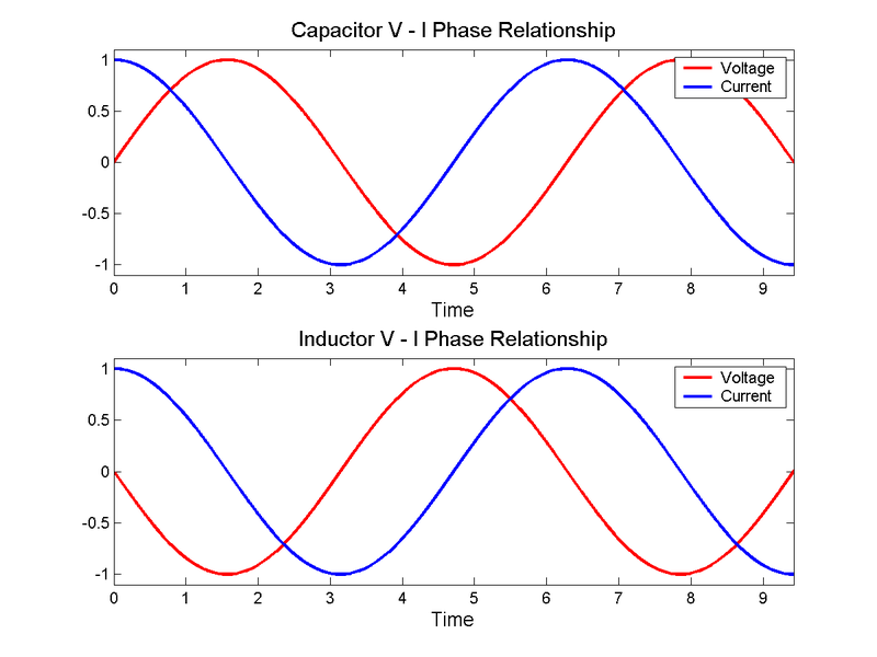
The metaphor of the stopwatch represents a periodic function. To be precise, it represents a sinusoid, i.e. a smooth repetitive oscillation. Now, the stopwatch hand represents the phase of that function, i.e. the φ angle in the illustration above. That angle is a function of time: the speed with which the stopwatch turns is related to some frequency, i.e. the number of oscillations per unit of time (i.e. per second).

You should now wonder: what frequency? What oscillations are we talking about here? Well… As we’re talking photons and electrons here, we should distinguish the two:

For photons, the frequency is given by Planck’s energy-frequency relation, which relates the energy (E) of a photon (1.5 to 3.5 eV for visible light) to its frequency (ν). It’s a simple proportional relation, with Planck’s constant (h) as the proportionality constant: E = hν, or ν = E/h.
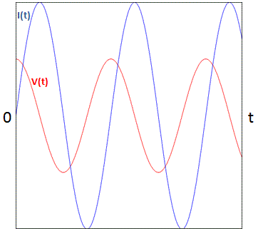
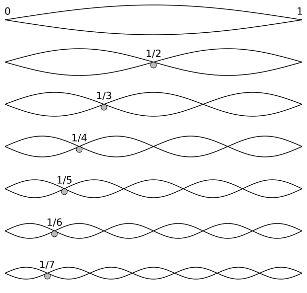
For electrons, we have the de Broglie relation, which looks similar to the Planck relation (E = hf, or f = E/h) but, as you know, it’s something different. Indeed, these so-called matter waves are not so easy to interpret because there actually is no precise frequency f. In fact, the matter wave representing some particle in space will consist of a potentially infinite number of waves, all superimposed one over another, as illustrated below.

For the sake of accuracy, I should mention that the animation above has its limitations: the wavetrain is complex-valued and, hence, has a real as well as an imaginary part, so it’s something like the blob underneath. Two functions in one, so to speak: the imaginary part follows the real part with a phase difference of 90 degrees (or π/2 radians). Indeed, if the wavefunction is a regular complex exponential re^iθ, then rsin(φ–π/2) = rcos(φ), which proves the point: we have two functions in one here. 🙂 I am actually just repeating what I said before already: the probability amplitude, or the wavefunction, is a complex number. You’ll usually see it written as Ψ (psi) or Φ (phi). Here also, using boldface (Ψ or Φ instead of Ψ or Φ) would usefully remind the reader that we’re talking something ‘two-dimensional’ (in mathematical space, that is), but this convention is usually not followed.

In any case… Back to frequencies. The point to note is that, when it comes to analyzing electrons (or any other matter-particle), we’re dealing with a range of frequencies f really (or, what amounts to the same, a range of wavelengths λ) and, hence, we should write Δf = ΔE/h, which is just one of the many expressions of the Uncertainty Principle in quantum mechanics.

Now, that’s just one of the complications. Another difficulty is that matter-particles, such as electrons, have some rest mass, and so that enters the energy equation as well (literally). Last but not least, one should distinguish between the group velocity and the phase velocity of matter waves. As you can imagine, that makes for a very complicated relationship between ‘the’ wavelength and ‘the’ frequency. In fact, what I write above should make it abundantly clear that there’s no such thing as the wavelength, or the frequency: it’s a range really, related to the fundamental uncertainty in quantum physics. I’ll come back to that, and so you shouldn’t worry about it here. Just note that the stopwatch metaphor doesn’t work very well for an electron!

In his postmortem lectures for Alix Mautner, Feynman avoids all these complications. Frankly, I think that’s a missed opportunity because I do not think it’s all that incomprehensible. In fact, I write all that follows because I do want you to understand the basics of waves. It’s not difficult. High-school math is enough here. Let’s go for it.

One turn of the stopwatch corresponds to one cycle. One cycle, or 1 Hz (i.e. one oscillation per second) covers 360 degrees or, to use a more natural unit, 2π radians. [Why is radian a more natural unit? Because it measures an angle in terms of the distance unit itself, rather than in arbitrary 1/360 cuts of a full circle. Indeed, remember that the circumference of the unit circle is 2π.] So our frequency ν (expressed in cycles per second) corresponds to a so-called angular frequency ω = 2πν. From this formula, it should be obvious that ω is measured in radians per second.

We can also link this formula to the period of the oscillation, T, i.e. the duration of one cycle. T = 1/ν and, hence, ω = 2π/T. It’s all nicely illustrated below. [And, yes, it’s an animation from Wikipedia: nice and simple.]

The easy math above now allows us to formally write the phase of a wavefunction – let’s denote the wavefunction as φ (phi), and the phase as θ (theta) – as a function of time (t) using the angular frequency ω. So we can write: θ = ωt = 2π·ν·t. Now, the wave travels through space, and the two illustrations above (i.e. the one with the super-imposed waves, and the one with the complex wave train) would usually represent a wave shape at some fixed point in time. Hence, the horizontal axis is not t but x. Hence, we can and should write the phase not only as a function of time but also of space. So how do we do that? Well… If the hypothesis is that the wave travels through space at some fixed speed c, then its frequency ν will also determine its wavelength λ. It’s a simple relationship: c = λν (the number of oscillations per second times the length of one wavelength should give you the distance traveled per second, so that’s, effectively, the wave’s speed).

Now that we’ve expressed the frequency in radians per second, we can also express the wavelength in radians per unit distance too. That’s what the wavenumber does: think of it as the spatial frequency of the wave. We denote the wavenumber by k, and write: k = 2π/λ. [Just do a numerical example when you have difficulty following. For example, if you’d assume the wavelength is 5 units distance (i.e. 5 meter) – that’s a typical VHF radio frequency: ν = (3×10⁸m/s)/(5 m) = 0.6×10⁸Hz = 60 MHz – then that would correspond to (2π radians)/(5 m) ≈ 1.2566 radians per meter. Of course, we can also express the wave number in oscillations per unit distance. In that case, we’d have to divide k by 2π, because one cycle corresponds to 2π radians. So we get the reciprocal of the wavelength: 1/λ. In our example, 1/λ is, of course, 1/5 = 0.2, so that’s a fifth of a full cycle. You can also think of it as the number of waves (or wavelengths) per meter: if the wavelength is λ, then one can fit 1/λ waves in a meter.

Now, from the ω = 2πν, c = λν and k = 2π/λ relations, it’s obvious that k = 2π/λ = 2π/(c/ν) = (2πν)/c = ω/c. To sum it all up, frequencies and wavelengths, in time and in space, are all related through the speed of propagation of the wave c. More specifically, they’re related as follows:

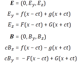
c = λν = ω/k

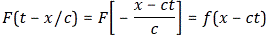
From that, it’s easy to see that k = ω/c, which we’ll use in a moment. Now, it’s obvious that the periodicity of the wave implies that we can find the same phase by going one oscillation (or a multiple number of oscillations back or forward in time, or in space. In fact, we can also find the same phase by letting both time and space vary. However, if we want to do that, it should be obvious that we should either (a) go forward in space and back in time or, alternatively, (b) go back in space and forward in time. In other words, if we want to get the same phase, then time and space sort of substitute for each other. Let me quote Feynman on this: “This is easily seen by considering the mathematical behavior of a. Evidently, if we add a little time , we get the same value for as we would have if we had subtracted a little distance: .” The variable a stands for the acceleration of an electric charge here, causing an electromagnetic wave, but the same logic is valid for the phase, with a minor twist though: we’re talking a nice periodic function here, and so we need to put the angular frequency in front. Hence, the rate of change of the phase in respect to time is measured by the angular frequency ω. In short, we write:

θ = ω(t–x/c) = ωt–kx

Hence, we can re-write the wavefunction, in terms of its phase, as follows:

φ(θ) = φ[θ(x, t)] = φ[ωt–kx]

Note that, if the wave would be traveling in the ‘other’ direction (i.e. in the negative x-direction), we’d write φ(θ) = φ[kx+ωt]. Time travels in one direction only, of course, but so one minus sign has to be there because of the logic involved in adding time and subtracting distance. You can work out an example (with a sine or cosine wave, for example) for yourself.

So what, you’ll say? Well… Nothing. I just hope you agree that all of this isn’t rocket science: it’s just high-school math. But so it shows you what that stopwatch really is and, hence, I – but who am I? – would have put at least one or two footnotes on this in a text like Feynman’s QED.

Now, let me make a much longer and more serious digression:

Digression 1: on relativity and spacetime

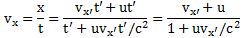
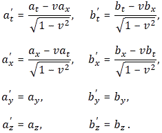
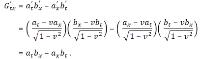
As you can see from the argument (or phase) of that wave function φ(θ) = φ[θ(x, t)] = φ[ωt–kx] = φ[–k(x–ct)], any wave equation establishes a deep relation between the wave itself (i.e. the ‘thing’ we’re describing) and space and time. In fact, that’s what the whole wave equation is all about! So let me say a few things more about that.

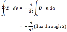
Because you know a thing or two about physics, you may ask: when we’re talking time, whose time are we talking about? Indeed, if we’re talking photons going from A to B, these photons will be traveling at or near the speed of light and, hence, their clock, as seen from our (inertial) frame of reference, doesn’t move. Likewise, according to the photon, our clock seems to be standing still.

Let me put the issue to bed immediately: we’re looking at things from our point of view. Hence, we’re obviously using our clock, not theirs. Having said that, the analysis is actually fully consistent with relativity theory. Why? Well… What do you expect? If it wasn’t, the analysis would obviously not be valid. 🙂 To illustrate that it’s consistent with relativity theory, I can mention, for example, that the (probability) amplitude for a photon to travel from point A to B depends on the spacetime interval, which is invariant. Hence, A and B are four-dimensional points in spacetime, involving both spatial as well as time coordinates: A = (x_A, y_A, z_A, t_A) and B = (x_B, y_B, z_B, t_B). And so the ‘distance’ – as measured through the spacetime interval – is invariant.

Now, having said that, we should draw some attention to the intimate relationship between space and time which, let me remind you, results from the absoluteness of the speed of light. Indeed, one will always measure the speed of light c as being equal to 299,792,458 m/s, always and everywhere. It does not depend on your reference frame (inertial or moving). That’s why the constant c anchors all laws in physics, and why we can write what we write above, i.e. include both distance (x) as well as time (t) in the wave function φ = φ(x, t) = φ[ωt–kx] = φ[–k(x–ct)]. The k and ω are related through the ω/k = c relationship: the speed of light links the frequency in time (ν = ω/2π = 1/T) with the frequency in space (i.e. the wavenumber or spatial frequency k). There is only degree of freedom here: the frequency—in space or in time, it doesn’t matter: ν and ω are not independent. [As noted above, the relationship between the frequency in time and in space is not so obvious for electrons, or for matter waves in general: for those matter-waves, we need to distinguish group and phase velocity, and so we don’t have a unique frequency.]

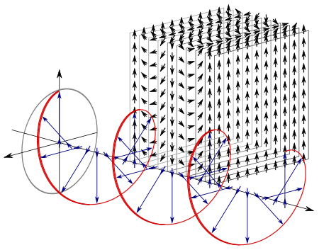
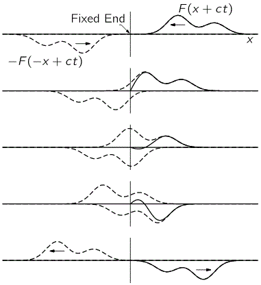
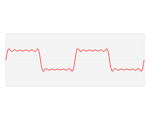
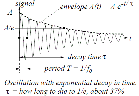
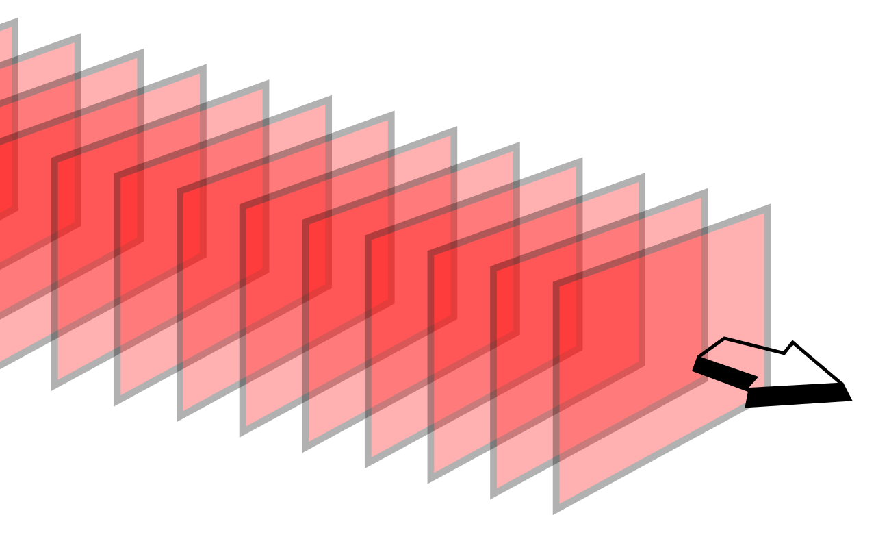
Let me make another small digression within the digression here. Thinking about travel at the speed of light invariably leads to paradoxes. In previous posts, I explained the mechanism of light emission: a photon is emitted – one photon only – when an electron jumps back to its ground state after being excited. Hence, we may imagine a photon as a transient electromagnetic wave–something like what’s pictured below. Now, the decay time of this transient oscillation (τ) is measured in nanoseconds, i.e. billionths of a second (1 ns = 1×10^–9s): the decay time for sodium light, for example, is some 30 ns only.

However, because of the tremendous speed of light, that still makes for a wavetrain that’s like ten meter long, at least (30×10^–9s times 3×10⁸m/s is nine meter, but you should note that the decay time measures the time for the oscillation to die out by a factor 1/e, so the oscillation itself lasts longer than that). Those nine or ten meters cover like 16 to 17 million oscillations (the wavelength of sodium light is about 600 nm and, hence, 10 meter fits almost 17 million oscillations indeed). Now, how can we reconcile the image of a photon as a ten-meter long wavetrain with the image of a photon as a point particle?

The answer to that question is paradoxical: from our perspective, anything traveling at the speed of light – including this nine or ten meter ‘long’ photon – will have zero length because of the relativistic length contraction effect. Length contraction? Yes. I’ll let you look it up, because… Well… It’s not easy to grasp. Indeed, from the three measurable effects on objects moving at relativistic speeds – i.e. (1) an increase of the mass (the energy needed to further accelerate particles in particle accelerators increases dramatically at speeds nearer to c), (2) time dilation, i.e. a slowing down of the (internal) clock (because of their relativistic speeds when entering the Earth’s atmosphere, the measured half-life of muons is five times that when at rest), and (3) length contraction – length contraction is probably the most paradoxical of all.

Let me end this digression with yet another short note. I said that one will always measure the speed of light c as being equal to 299,792,458 m/s, always and everywhere and, hence, that it does not depend on your reference frame (inertial or moving). Well… That’s true and not true at the same time. I actually need to nuance that statement a bit in light of what follows: an individual photon does have an amplitude to travel faster or slower than c, and when discussing matter waves (such as the wavefunction that’s associated with an electron), we can have phase velocities that are faster than light! However, when calculating those amplitudes, c is a constant.

That doesn’t make sense, you’ll say. Well… What can I say? That’s how it is unfortunately. I need to move on and, hence, I’ll end this digression and get back to the main story line. Part I explained what probability amplitudes are—or at least tried to do so. Now it’s time for part II: the building blocks of all of quantum electrodynamics (QED).

II. The building blocks: P(A to B), E(A to B) and j

The three basic ‘events’ (and, hence, amplitudes) in QED are the following:

1. P(A to B)

P(A to B) is the (probability) amplitude for a photon to travel from point A to B. However, I should immediately note that A and B are points in spacetime. Therefore, we associate them not only with some specific (x, y, z) position in space, but also with a some specific time t. Now, quantum-mechanical theory gives us an easy formula for P(A to B): it depends on the so-called (spacetime) interval between the two points A and B, i.e. I = Δr²– Δt²= (x₂–x₁)²+(y₂–y₁)²+(z₂–z₁)²– (t₂–t₁)². The point to note is that the spacetime interval takes both the distance in space as well as the ‘distance’ in time into account. As I mentioned already, this spacetime interval does not depend on our reference frame and, hence, it’s invariant (as long as we’re talking reference frames that move with constant speed relative to each other). Also note that we should measure time and distance in equivalent units when using that Δr²– Δt²formula for I. So we either measure distance in light-seconds or, else, we measure time in units that correspond to the time that’s needed for light to travel one meter. If no equivalent units are adopted, the formula is I = Δr²– c·Δt².

Now, in quantum theory, anything is possible and, hence, not only do we allow for crooked paths, but we also allow for the difference in time to differ from the time you’d expect a photon to need to travel along some curve (whose length we’ll denote by l), i.e. l/c. Hence, our photon may actually travel slower or faster than the speed of light c! There is one lucky break, however, that makes all come out alright: it’s easy to show that the amplitudes associated with the odd paths and strange timings generally cancel each other out. [That’s what the QED booklet shows.] Hence, what remains, are the paths that are equal or, importantly, those that very near to the so-called ‘light-like’ intervals in spacetime only. The net result is that light – even one single photon – effectively uses a (very) small core of space as it travels, as evidenced by the fact that even one single photon interferes with itself when traveling through a slit or a small hole!

[If you now wonder what it means for a photon to interfere for itself, let me just give you the easy explanation: it may change its path. We assume it was traveling in a straight line – if only because it left the source at some point in time and then arrived at the slit obviously – but so it no longer travels in a straight line after going through the slit. So that’s what we mean here.]

2. E(A to B)

E(A to B) is the (probability) amplitude for an electron to travel from point A to B. The formula for E(A to B) is much more complicated, and it’s the one I want to discuss somewhat more in detail in this post. It depends on some complex number j (see the next remark) and some real number n.

3. j

Finally, an electron could emit or absorb a photon, and the amplitude associated with this event is denoted by j, for junction number. It’s the same number j as the one mentioned when discussing E(A to B) above.

Now, this junction number is often referred to as the coupling constant or the fine-structure constant. However, the truth is, as I pointed out in my previous post, that these numbers are related, but they are not quite the same: α is the square of j, so we have α = j². There is also one more, related, number: the gauge parameter, which is denoted by g (despite the g notation, it has nothing to do with gravitation). The value of g is the square root of 4πε₀α, so g²= 4πε₀α. I’ll come back to this. Let me first make an awfully long digression on the fine-structure constant. It will be awfully long. So long that it’s actually part of the ‘core’ of this post actually.

Digression 2: on the fine-structure constant, Planck units and the Bohr radius

The value for j is approximately –0.08542454.

How do we know that?

The easy answer to that question is: physicists measured it. In fact, they usually publish the measured value as the square root of the (absolute value) of j, which is that fine-structure constant α. Its value is published (and updated) by the US National Institute on Standards and Technology. To be precise, the currently accepted value of α is 7.29735257×10⁻³. In case you doubt, just check that square root:

j = –0.08542454 ≈ –√0.00729735257 = –√α

As noted in Feynman’s (or Leighton’s) QED, older and/or more popular books will usually mention 1/α as the ‘magical’ number, so the ‘special’ number you may have seen is the inverse fine-structure constant, which is about 137, but not quite:

1/α = 137.035999074 ± 0.000000044

I am adding the standard uncertainty just to give you an idea of how precise these measurements are. 🙂 About 0.32 parts per billion (just divide the 137.035999074 number by the uncertainty). So that‘s the number that excites popular writers, including Leighton. Indeed, as Leighton puts it:

“Where does this number come from? Nobody knows. It’s one of the greatest damn mysteries of physics: a magic number that comes to us with no understanding by man. You might say the “hand of God” wrote that number, and “we don’t know how He pushed his pencil.” We know what kind of a dance to do experimentally to measure this number very accurately, but we don’t know what kind of dance to do on the computer to make this number come out, without putting it in secretly!”

Is it Leighton, or did Feynman really say this? Not sure. While the fine-structure constant is a very special number, it’s not the only ‘special’ number. In fact, we derive it from other ‘magical’ numbers. To be specific, I’ll show you how we derive it from the fundamental properties – as measured, of course – of the electron. So, in fact, I should say that we do know how to make this number come out, which makes me doubt whether Feynman really said what Leighton said he said. 🙂

So we can derive α from some other numbers. That brings me to the more complicated answer to the question as to what the value of j really is: j‘s value is the electron charge expressed in Planck units, which I’ll denote by –e_P:

j = –e_P

[You may want to reflect on this, and quickly verify on the Web. The Planck unit of electric charge, expressed in Coulomb, is about 1.87555×10^–18C. If you multiply that j = –e_P, so with –0.08542454, you get the right answer: the electron charge is about –0.160217×10^–18C.]

Now that is strange.

Why? Well… For starters, when doing all those quantum-mechanical calculations, we like to think of j as a dimensionless number: a coupling constant. But so here we do have a dimension: electric charge.

Let’s look at the basics. If j is –√α, and it’s also equal to –e_P, then the fine-structure constant must also be equal to the square of the electron charge e_P, so we can write:

α = e_P²

You’ll say: yes, so what? Well… I am pretty sure that, if you’ve ever seen a formula for α, it’s surely not this simple j = –e_P or α = e_P² formula. What you’ve seen, most likely, is one or more of the following expressions below :

That’s a pretty impressive collection of physical constants, isn’t it? 🙂 They’re all different but, somehow, when we combine them in one or the other ratio (we have not less than five different expressions here (each identity is a separate expression), and I could give you a few more!), we get the very same number: α. Now that is what I call strange. Truly strange. Incomprehensibly weird!

You’ll say… Well… Those constants must all be related… Of course! That’s exactly the point I am making here. They are, but look how different they are: m_emeasures mass, r_emeasures distance, e is a charge, and so these are all very different numbers with very different dimensions. Yet, somehow, they are all related through this α number. Frankly, I do not know of any other expression that better illustrates some kind of underlying unity in Nature than the one with those five identities above.

Let’s have a closer look at those constants. You know most of them already. The only constants you may not have seen before are μ₀, R_Kand, perhaps, r_eas well as m_e. However, these can easily be defined as some easy function of the constants that you did see before, so let me quickly do that:

The μ₀ constant is the so-called magnetic constant. It’s something similar as ε₀ and it’s referred to as the magnetic permeability of the vacuum. So it’s just like the (electric) permittivity of the vacuum (i.e. the electric constant ε₀) and the only reason why this blog hasn’t mentioned this constant before is because I haven’t really discussed magnetic fields so far. I only talked about the electric field vector. In any case, you know that the electric and magnetic force are part and parcel of the same phenomenon (i.e. the electromagnetic interaction between charged particles) and, hence, they are closely related. To be precise, μ₀ε₀ = 1/c²= c^–2. So that shows the first and second expression for α are, effectively, fully equivalent. [Just in case you’d doubt that μ₀ε₀ = 1/c², let me give you the values: μ₀ = 4π·10^–7N/A², and ε₀ = (1/4π·c²)·10⁷C²/N·m². Just plug them in, and you’ll see it’s bang on. Moreover, note that the ampere (A) unit is equal to the coulomb per second unit (C/s), so even the units come out alright. 🙂 Of course they do!]
The k_e constant is the Coulomb constant and, from its definition k_e = 1/4πε₀, it’s easy to see how those two expressions are, in turn, equivalent with the third expression for α.
The R_Kconstant is the so-called von Klitzing constant. Huh? Yes. I know. I am pretty sure you’ve never ever heard of that one before. Don’t worry about it. It’s, quite simply, equal to R_K= h/e². Hence, substituting (and don’t forget that h = 2πħ) will demonstrate the equivalence of the fourth expression for α.
Finally, the r_e factor is the classical electron radius, which is usually written as a function of m_e, i.e. the electron mass: r_e = e²/4πε₀m_ec². Also note that this also implies that r_em_e = e²/4πε₀c². In words: the product of the electron mass and the electron radius is equal to some constant involving the electron (e), the electric constant (ε₀), and c (the speed of light).

I am sure you’re under some kind of ‘formula shock’ now. But you should just take a deep breath and read on. The point to note is that all these very different things are all related through α.

So, again, what is that α really? Well… A strange number indeed. It’s dimensionless (so we don’t measure in kg, m/s, eV·s or whatever) and it pops up everywhere. [Of course, you’ll say: “What’s everywhere? This is the first time I‘ve heard of it!” :-)]

Well… Let me start by explaining the term itself. The fine structure in the name refers to the splitting of the spectral lines of atoms. That’s a very fine structure indeed. 🙂 We also have a so-called hyperfine structure. Both are illustrated below for the hydrogen atom. The numbers n, J, I, and F are quantum numbers used in the quantum-mechanical explanation of the emission spectrum, which is also depicted below, but note that the illustration gives you the so-called Balmer series only, i.e. the colors in the visible light spectrum (there are many more ‘colors’ in the high-energy ultraviolet and the low-energy infrared range).

To be precise: (1) n is the principal quantum number: here it takes the values 1 or 2, and we could say these are the principal shells; (2) the S, P, D,… orbitals (which are usually written in lower case: s, p, d, f, g, h and i) correspond to the (orbital) angular momentum quantum number l = 0, 1, 2,…, so we could say it’s the subshell; (3) the J values correspond to the so-called magnetic quantum number m, which goes from –l to +l; (4) the fourth quantum number is the spin angular momentum s. I’ve copied another diagram below so you see how it works, more or less, that is.

Now, our fine-structure constant is related to these quantum numbers. How exactly is a bit of a long story, and so I’ll just copy Wikipedia’s summary on this: ” The gross structure of line spectra is the line spectra predicted by the quantum mechanics of non-relativistic electrons with no spin. For a hydrogenic atom, the gross structure energy levels only depend on the principal quantum number n. However, a more accurate model takes into account relativistic and spin effects, which break the degeneracy of the the energy levels and split the spectral lines. The scale of the fine structure splitting relative to the gross structure energies is on the order of (Zα)², where Z is the atomic number and α is the fine-structure constant.” There you go. You’ll say: so what? Well… Nothing. If you aren’t amazed by that, you should stop reading this.

It is an ‘amazing’ number, indeed, and, hence, it does quality for being “one of the greatest damn mysteries of physics”, as Feynman and/or Leighton put it. Having said that, I would not go as far as to write that it’s “a magic number that comes to us with no understanding by man.” In fact, I think Feynman/Leighton could have done a much better job when explaining what it’s all about. So, yes, I hope to do better than Leighton here and, as he’s still alive, I actually hope he reads this. 🙂

The point is: α is not the only weird number. What’s particular about it, as a physical constant, is that it’s dimensionless, because it relates a number of other physical constants in such a way that the units fall away. Having said that, the Planck or Boltzmann constant are at least as weird.

So… What is this all about? Well… You’ve probably heard about the so-called fine-tuning problem in physics and, if you’re like me, your first reaction will be to associate fine-tuning with fine-structure. However, the two terms have nothing in common, except for four letters. 🙂 OK. Well… I am exaggerating here. The two terms are actually related, to some extent at least, but let me explain how.

The term fine-tuning refers to the fact that all the parameters or constants in the so-called Standard Model of physics are, indeed, all related to each other in the way they are. We can’t sort of just turn the knob of one and change it, because everything falls apart then. So, in essence, the fine-tuning problem in physics is more like a philosophical question: why is the value of all these physical constants and parameters exactly what it is? So it’s like asking: could we change some of the ‘constants’ and still end up with the world we’re living in? Or, if it would be some different world, how would it look like? What if c was some other number? What if k_e or ε₀ was some other number? In short, and in light of those expressions for α, we may rephrase the question as: why is α what is is?

Of course, that’s a question one shouldn’t try to answer before answering some other, more fundamental, question: how many degrees of freedom are there really? Indeed, we just saw that k_e and ε₀are intimately related through some equation, and other constants and parameters are related too. So the question is like: what are the ‘dependent’ and the ‘independent’ variables in this so-called Standard Model?

There is no easy answer to that question. In fact, one of the reasons why I find physics so fascinating is that one cannot easily answer such questions. There are the obvious relationships, of course. For example, the k_e = 1/4πε₀relationship, and the context in which they are used (Coulomb’s Law) does, indeed, strongly suggest that both constants are actually part and parcel of the same thing. Identical, I’d say. Likewise, the μ₀ε₀ = 1/c²relation also suggests there’s only one degree of freedom here, just like there’s only one degree of freedom in that ω/k = c relationship (if we set a value for ω, we have k, and vice versa). But… Well… I am not quite sure how to phrase this, but… What physical constants could be ‘variables’ indeed?

It’s pretty obvious that the various formulas for α cannot answer that question: you could stare at them for days and weeks and months and years really, but I’d suggest you use your time to read more of Feynman’s real Lectures instead. 🙂 One point that may help to come to terms with this question – to some extent, at least – is what I casually mentioned above already: the fine-structure constant is equal to the square of the electron charge expressed in Planck units: α = e_P².

Now, that’s very remarkable because Planck units are some kind of ‘natural units’ indeed (for the detail, see my previous post: among other things, it explains what these Planck units really are) and, therefore, it is quite tempting to think that we’ve actually got only one degree of freedom here: α itself. All the rest should follow from it.

[…]

It should… But… Does it?

The answer is: yes and no. To be frank, it’s more no than yes because, as I noted a couple of times already, the fine-structure constant relates a lot of stuff but it’s surely not the only significant number in the Universe. For starters, I said that our E(A to B) formula has two ‘variables’:

We have that complex number j, which, as mentioned, is equal to the electron charge expressed in Planck units. [In case you wonder why –e_P ≈ –0.08542455 is said to be an amplitude, i.e. a complex number or an ‘arrow’… Well… Complex numbers include the real numbers and, hence, –0.08542455 is both real and complex. When combining ‘arrows’ or, to be precise, when multiplying some complex number with –0.08542455, we will (a) shrink the original arrow to about 8.5% of its original value (8.542455% to be precise) and (b) rotate it over an angle of plus or minus 180 degrees. In other words, we’ll reverse its direction. Hence, using Euler’s notation for complex numbers, we can write: –1 = e^iπ= e^–iπ and, hence, –0.085 = 0.085·e^iπ= 0.085·e^–iπ. So, in short, yes, j is a complex number, or an ‘arrow’, if you prefer that term.]
We also have some some real number n in the E(A to B) formula. So what’s the n? Well… Believe it or not, it’s the electron mass! Isn’t that amazing?

You’ll say: “Well… Hmm… I suppose so.” But then you may – and actually should – also wonder: the electron mass? In what units? Planck units again? And are we talking relativistic mass (i.e. its total mass, including the equivalent mass of its kinetic energy) or its rest mass only? And we were talking α here, so can we relate it to α too, just like the electron charge?

These are all very good questions. Let’s start with the second one. We’re talking rather slow-moving electrons here, so the relativistic mass (m) and its rest mass (m₀) is more or less the same. Indeed, the Lorentz factor γ in the m = γm₀ equation is very close to 1 for electrons moving at their typical speed. So… Well… That question doesn’t matter very much. Really? Yes. OK. Because you’re doubting, I’ll quickly show it to you. What is their ‘typical’ speed?

We know we shouldn’t attach too much importance to the concept of an electron in orbit around some nucleus (we know it’s not like some planet orbiting around some star) and, hence, to the concept of speed or velocity (velocity is speed with direction) when discussing an electron in an atom. The concept of momentum (i.e. velocity combined with mass or energy) is much more relevant. There’s a very easy mathematical relationship that gives us some clue here: the Uncertainty Principle. In fact, we’ll use the Uncertainty Principle to relate the momentum of an electron (p) to the so-called Bohr radius r (think of it as the size of a hydrogen atom) as follows: p ≈ ħ/r. [I’ll come back on this in a moment, and show you why this makes sense.]

Now we also know its kinetic energy (K.E.) is mv²/2, which we can write as p²/2m. Substituting our p ≈ ħ/r conjecture, we get K.E. = mv²/2 = ħ²/2mr². This is equivalent to m²v² = ħ²/r²(just multiply both sides with m). From that, we get v = ħ/mr. Now, one of the many relations we can derive from the formulas for the fine-structure constant is r_e = α²r. [I haven’t showed you that yet, but I will shortly. It’s a really amazing expression. However, as for now, just accept it as a simple formula for interim use in this digression.] Hence, r = r_e/α². The r_efactor in this expression is the so-called classical electron radius. So we can now write v = ħα²/mr_e. Let’s now throw c in: v/c = α²ħ/mcr_e. However, from that fifth expression for α, we know that ħ/mcr_e = α, so we get v/c = α. We have another amazing result here: the v/c ratio for an electron (i.e. its speed expressed as a fraction of the speed of light) is equal to that fine-structure constant α. So that’s about 1/137, so that’s less than 1% of the speed of light. Now… I’ll leave it to you to calculate the Lorentz factor γ but… Well… It’s obvious that it will be very close to 1. 🙂 Hence, the electron’s speed – however we want to visualize that – doesn’t matter much indeed, so we should not worry about relativistic corrections in the formulas.

Let’s now look at the question in regard to the Planck units. If you know nothing at all about them, I would advise you to read what I wrote about them in my previous post. Let me just note we get those Planck units by equating not less than five fundamental physical constants to 1, notably (1) the speed of light, (2) Planck’s (reduced) constant, (3) Boltzmann’s constant, (4) Coulomb’s constant and (5) Newton’s constant (i.e. the gravitational constant). Hence, we have a set of five equations here (c = ħ = k_B = k_e = G = 1), and so we can solve that to get the five Planck units, i.e. the Planck length unit, the Planck time unit, the Planck mass unit, the Planck energy unit, the Planck charge unit and, finally (oft forgotten), the Planck temperature unit. Of course, you should note that all mass and energy units are directly related because of the mass-energy equivalence relation E = mc², which simplifies to E = m if c is equated to 1. [I could also say something about the relation between temperature and (kinetic) energy, but I won’t, as it would only further confuse you.]

Now, you may or may not remember that the Planck time and length units are unimaginably small, but that the Planck mass unit is actually quite sizable—at the atomic scale, that is. Indeed, the Planck mass is something huge, like the mass of an eyebrow hair, or a flea egg. Is that huge? Yes. Because if you’d want to pack it in a Planck-sized particle, it would make for a tiny black hole. 🙂 No kidding. That’s the physical significance of the Planck mass and the Planck length and, yes, it’s weird. 🙂

Let me give you some values. First, the Planck mass itself: it’s about 2.1765×10⁻⁸kg. Again, if you think that’s tiny, think again. From the E = mc² equivalence relationship, we get that this is equivalent to 2 giga-joule, approximately. Just to give an idea, that’s like the monthly electricity consumption of an average American family. So that’s huge indeed! 🙂 [Many people think that nuclear energy involves the conversion of mass into energy, but the story is actually more complicated than that. In any case… I need to move on.]

Let me now give you the electron mass expressed in the Planck mass unit:

Measured in our old-fashioned super-sized SI kilogram unit, the electron mass is m_e = 9.1×10^–31kg.
The Planck mass is m_P = 2.1765×10⁻⁸kg.
Hence, the electron mass expressed in Planck units is m_{e_P} = m_e/m_P = (9.1×10^–31kg)/(2.1765×10⁻⁸kg) = 4.181×10⁻²³.

We can, once again, write that as some function of the fine-structure constant. More specifically, we can write:

m_{e_P} = α/r_{e_P} = α/α²r_P = 1/αr_P

So… Well… Yes: yet another amazing formula involving α.

In this formula, we have r_{e_P} and r_P, which are the (classical) electron radius and the Bohr radius expressed in Planck (length) units respectively. So you can see what’s going on here: we have all kinds of numbers here expressed in Planck units: a charge, a radius, a mass,… And we can relate all of them to the fine-structure constant.

Why? Who knows? I don’t. As Leighton puts it: that’s just the way “God pushed His pencil.” 🙂

Note that the beauty of natural units ensures that we get the same number for the (equivalent) energy of an electron. Indeed, from the E = mc² relation, we know the mass of an electron can also be written as 0.511 MeV/c². Hence, the equivalent energy is 0.511 MeV (so that’s, quite simply, the same number but without the 1/c²factor). Now, the Planck energy E_P (in eV) is 1.22×10²⁸eV, so we get E_{e_P} = E_e/E_P= (0.511×10⁶eV)/(1.22×10²⁸eV) = 4.181×10⁻²³. So it’s exactly the same as the electron mass expressed in Planck units. Isn’t that nice? 🙂

Now, are all these numbers dimensionless, just like α? The answer to that question is complicated. Yes, and… Well… No:

Yes. They’re dimensionless because they measure something in natural units, i.e. Planck units, and, hence, that’s some kind of relative measure indeed so… Well… Yes, dimensionless.
No. They’re not dimensionless because they do measure something, like a charge, a length, or a mass, and when you chose some kind of relative measure, you still need to define some gauge, i.e. some kind of standard measure. So there’s some ‘dimension’ involved there.

So what’s the final answer? Well… The Planck units are not dimensionless. All we can say is that they are closely related, physically. I should also add that we’ll use the electron charge and mass (expressed in Planck units) in our amplitude calculations as a simple (dimensionless) number between zero and one. So the correct answer to the question as to whether these numbers have any dimension is: expressing some quantities in Planck units sort of normalizes them, so we can use them directly in dimensionless calculations, like when we multiply and add amplitudes.

Hmm… Well… I can imagine you’re not very happy with this answer but it’s the best I can do. Sorry. I’ll let you further ponder that question. I need to move on.

Note that that 4.181×10⁻²³ is still a very small number (23 zeroes after the decimal point!), even if it’s like 46 million times larger than the electron mass measured in our conventional SI unit (i.e. 9.1×10^–31kg). Does such small number make any sense? The answer is: yes, it does. When we’ll finally start discussing that E(A to B) formula (I’ll give it to you in a moment), you’ll see that a very small number for n makes a lot of sense.

Before diving into it all, let’s first see if that formula for that alpha, that fine-structure constant, still makes sense with m_e expressed in Planck units. Just to make sure. 🙂 To do that, we need to use the fifth (last) expression for a, i.e. the one with r_e in it. Now, in my previous post, I also gave some formula for r_e: r_e = e²/4πε₀m_ec², which we can re-write as r_em_e = e²/4πε₀c². If we substitute that expression for r_em_e in the formula for α, we can calculate α from the electron charge, which indicates both the electron radius and its mass are not some random God-given variable, or “some magic number that comes to us with no understanding by man“, as Feynman – well… Leighton, I guess – puts it. No. They are magic numbers alright, one related to another through the equally ‘magic’ number α, but so I do feel we actually can create some understanding here.

At this point, I’ll digress once again, and insert some quick back-of-the-envelope argument from Feynman’s very serious Caltech Lectures on Physics, in which, as part of the introduction to quantum mechanics, he calculates the so-called Bohr radius from Planck’s constant h. Let me quickly explain: the Bohr radius is, roughly speaking, the size of the simplest atom, i.e. an atom with one electron (so that’s hydrogen really). So it’s not the classical electron radius r_e. However, both are also related to that ‘magical number’ α. To be precise, if we write the Bohr radius as r, then r_e = α²r ≈ 0.000053… times r, which we can re-write as:

α = √(r_e /r) = (r_e /r)^1/2

So that’s yet another amazing formula involving the fine-structure constant. In fact, it’s the formula I used as an ‘interim’ expression to calculate the relative speed of electrons. I just used it without any explanation there, but I am coming back to it here. Alpha again…

Just think about it for a while. In case you’d still doubt the magic of that number, let me write what we’ve discovered so far:

(1) α is the square of the electron charge expressed in Planck units: α = e_P².

(2) α is the square root of the ratio of (a) the classical electron radius and (b) the Bohr radius: α = √(r_e /r). You’ll see this more often written as r_e = α²r. Also note that this is an equation that does not depend on the units, in contrast to equation 1 (above), and 4 and 5 (below), which require you to switch to Planck units. It’s the square of a ratio and, hence, the units don’t matter. They fall away.

(3) α is the (relative) speed of an electron: α = v/c. [The relative speed is the speed as measured against the speed of light. Note that the ‘natural’ unit of speed in the Planck system of units is equal to c. Indeed, if you divide one Planck length by one Planck time unit, you get (1.616×10⁻³⁵m)/(5.391×10⁻⁴⁴s) = c m/s. However, this is another equation, just like (2), that does not depend on the units: we can express v and c in whatever unit we want, as long we’re consistent and express both in the same units.]

(4) Finally – I’ll show you in a moment – α is also equal to the product of (a) the electron mass (which I’ll simply write as m_e here) and (b) the classical electron radius r_e (if both are expressed in Planck units): α = m_e·r_e. Now I think that’s, perhaps, the most amazing of all of the expressions for α. If you don’t think that’s amazing, I’d really suggest you stop trying to study physics. 🙂

Note that, from (2) and (4), we find that:

(5) The electron mass (in Planck units) is equal m_e = α/r_e= α/α²r = 1/αr. So that gives us an expression, using α once again, for the electron mass as a function of the Bohr radius r expressed in Planck units.

Finally, we can also substitute (1) in (5) to get:

(6) The electron mass (in Planck units) is equal to m_e = α/r_e = e_P²/r_e. Using the Bohr radius, we get m_e = 1/αr = 1/e_P²r.

So… As you can see, this fine-structure constant really links ALL of the fundamental properties of the electron: its charge, its radius, its distance to the nucleus (i.e. the Bohr radius), its velocity, its mass (and, hence, its energy),… In short,

IT IS ALL IN ALPHA!

Now that should answer the question in regard to the degrees of freedom we have here, doesn’t it? It looks like we’ve got only one degree of freedom here. Indeed, if we’ve got some value for α, then we’ve have the electron charge, and from the electron charge, we can calculate the Bohr radius r (as I will show below), and if we have r, we have m_eand r_e. And then we can also calculate v, which gives us its momentum (mv) and its kinetic energy (mv²/2). In short,

ALPHA GIVES US EVERYTHING!

Isn’t that amazing? Hmm… You should reserve your judgment as for now, and carefully go over all of the formulas above and verify my statement. If you do that, you’ll probably struggle to find the Bohr radius from the charge (i.e. from α). So let me show you how you do that, because it will also show you why you should, indeed, reserve your judgment. In other words, I’ll show you why alpha does NOT give us everything! The argument below will, finally, prove some of the formulas that I didn’t prove above. Let’s go for it:

1. If we assume that (a) an electron takes some space – which I’ll denote by r 🙂 – and (b) that it has some momentum p because of its mass m and its velocity v, then the ΔxΔp = ħ relation (i.e. the Uncertainty Principle in its roughest form) suggests that the order of magnitude of r and p should be related in the very same way. Hence, let’s just boldly write r ≈ ħ/p and see what we can do with that. So we equate Δx with r and Δp with p. As Feynman notes, this is really more like a ‘dimensional analysis’ (he obviously means something very ‘rough’ with that) and so we don’t care about factors like 2 or 1/2. [Indeed, note that the more precise formulation of the Uncertainty Principle is σ_xσ_p≥ ħ/2.] In fact, we didn’t even bother to define r very rigorously. We just don’t care about precise statements at this point. We’re only concerned about orders of magnitude. [If you’re appalled by the rather rude approach, I am sorry for that, but just try to go along with it.]

2. From our discussions on energy, we know that the kinetic energy is mv²/2, which we can write as p²/2m so we get rid of the velocity factor. [Why? Because we can’t really imagine what it is anyway. As I said a couple of times already, we shouldn’t think of electrons as planets orbiting around some star. That model doesn’t work.] So… What’s next? Well… Substituting our p ≈ ħ/r conjecture, we get K.E. = ħ²/2mr². So that’s a formula for the kinetic energy. Next is potential.

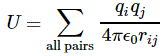
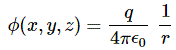
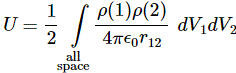
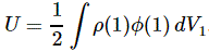
3. Unfortunately, the discussion on potential energy is a bit more complicated. You’ll probably remember that we had an easy and very comprehensible formula for the energy that’s needed (i.e. the work that needs to be done) to bring two charges together from a large distance (i.e. infinity). Indeed, we derived that formula directly from Coulomb’s Law (and Newton’s law of force) and it’s U = q₁q₂/4πε₀r₁₂. [If you think I am going too fast, sorry, please check for yourself by reading my other posts.] Now, we’re actually talking about the size of an atom here in my previous post, so one charge is the proton (+e) and the other is the electron (–e), so the potential energy is U = P.E. = –e²/4πε₀r, with r the ‘distance’ between the proton and the electron—so that’s the Bohr radius we’re looking for!

[In case you’re struggling a bit with those minus signs when talking potential energy – I am not ashamed to admit I did! – let me quickly help you here. It has to do with our reference point: the reference point for measuring potential energy is at infinity, and it’s zero there (that’s just our convention). Now, to separate the proton and the electron, we’d have to do quite a lot of work. To use an analogy: imagine we’re somewhere deep down in a cave, and we have to climb back to the zero level. You’ll agree that’s likely to involve some sweat, don’t you? Hence, the potential energy associated with us being down in the cave is negative. Likewise, if we write the potential energy between the proton and the electron as U(r), and the potential energy at the reference point as U(∞) = 0, then the work to be done to separate the charges, i.e. the potential difference U(∞) – U(r), will be positive. So U(∞) – U(r) = 0 – U(r) > 0 and, hence, U(r) < 0. If you still don’t ‘get’ this, think of the electron being in some (potential) well, i.e. below the zero level, and so it’s potential energy is less than zero. Huh? Sorry. I have to move on. :-)]

4. We can now write the total energy (which I’ll denote by E, but don’t confuse it with the electric field vector!) as

E = K.E. + P.E. = ħ²/2mr²– e²/4πε₀r

Now, the electron (whatever it is) is, obviously, in some kind of equilibrium state. Why is that obvious? Well… Otherwise our hydrogen atom wouldn’t or couldn’t exist. 🙂 Hence, it’s in some kind of energy ‘well’ indeed, at the bottom. Such equilibrium point ‘at the bottom’ is characterized by its derivative (in respect to whatever variable) being equal to zero. Now, the only ‘variable’ here is r (all the other symbols are physical constants), so we have to solve for dE/dr = 0. Writing it all out yields:

dE/dr = –ħ²/mr³+ e²/4πε₀r²= 0 ⇔ r = 4πε₀ħ²/me²

You’ll say: so what? Well… We’ve got a nice formula for the Bohr radius here, and we got it in no time! 🙂 But the analysis was rough, so let’s check if it’s any good by putting the values in:

r = 4πε₀h²/me²

= [(1/(9×10⁹) C²/N·m²)·(1.055×10^–34J·s)²]/[(9.1×10^–31kg)·(1.6×10^–19C)²]

= 53×10^–12m = 53 pico-meter (pm)

So what? Well… Double-check it on the Internet: the Bohr radius is, effectively, about 53 trillionths of a meter indeed! So we’re right on the spot!

[In case you wonder about the units, note that mass is a measure of inertia: one kg is the mass of an object which, subject to a force of 1 newton, will accelerate at the rate of 1 m/s per second. Hence, we write F = m·a, which is equivalent to m = F/a. Hence, the kg, as a unit, is equivalent to 1 N/(m/s²). If you make this substitution, we get r in the unit we want to see: [(C²/N·m²)·(N²·m²·s²)/[(N·s²/m)·C²] = m.]

Moreover, if we take that value for r and put it in the (total) energy formula above, we’d find that the energy of the electron is –13.6 eV. [Don’t forget to convert from joule to electronvolt when doing the calculation!] Now you can check that on the Internet too: 13.6 eV is exactly the amount of energy that’s needed to ionize a hydrogen atom (i.e. the energy that’s needed to kick the electron out of that energy well)!

Waw ! Isn’t it great that such simple calculations yield such great results? 🙂 [Of course, you’ll note that the omission of the 1/2 factor in the Uncertainty Principle was quite strategic. :-)] Using the r = 4πε₀ħ²/me²formula for the Bohr radius, you can now easily check the r_e = α²r formula. You should find what we jotted down already: the classical electron radius is equal to r_e = e²/4πε₀m_ec². To be precise, r_e = (53×10^–6)·(53×10^–12m) = 2.8×10^–15m. Now that’s again something you should check on the Internet. Guess what? […] It’s right on the spot again. 🙂

We can now also check that α = m·r_e formula: α = m·r_e= 4.181×10⁻²³times… Hey! Wait! We have to express r_ein Planck units as well, of course! Now, (2.81794×10^–15m)/(1.616×10^–35m) ≈ 1.7438 ×10²⁰. So now we get 4.181×10⁻²³times 1.7438×10²⁰= 7.29×10^–3= 0.00729 ≈ 1/137. Bingo! We got the magic number once again. 🙂

So… Well… Doesn’t that confirm we actually do have it all with α?

Well… Yes and no… First, you should note that I had to use h in that calculation of the Bohr radius. Moreover, the other physical constants (most notably c and the Coulomb constant) were actually there as well, ‘in the background’ so to speak, because one needs them to derive the formulas we used above. And then we have the equations themselves, of course, most notably that Uncertainty Principle… So… Well…

It’s not like God gave us one number only (α) and that all the rest flows out of it. We have a whole bunch of ‘fundamental’ relations and ‘fundamental’ constants here.

Having said that, it’s true that statement still does not diminish the magic of alpha.

Hmm… Now you’ll wonder: how many? How many constants do we need in all of physics?

Well… I’d say, you should not only ask about the constants: you should also ask about the equations: how many equations do we need in all of physics? [Just for the record, I had to smile when the Hawking of the movie says that he’s actually looking for one formula that sums up all of physics. Frankly, that’s a nonsensical statement. Hence, I think the real Hawking never said anything like that. Or, if he did, that it was one of those statements one needs to interpret very carefully.]

But let’s look at a few constants indeed. For example, if we have c, h and α, then we can calculate the electric charge e and, hence, the electric constant ε₀= e²/2αhc. From that, we get Coulomb’s constant k_e, because k_e is defined as 1/4πε₀… But…

Hey! Wait a minute! How do we know that k_e = 1/4πε₀? Well… From experiment. But… Yes? That means 1/4π is some fundamental proportionality coefficient too, isn’t it?

Wow! You’re smart. That’s a good and valid remark. In fact, we use the so-called reduced Planck constant ħ in a number of calculations, and so that involves a 2π factor too (ħ = h/2π). Hence… Well… Yes, perhaps we should consider 2π as some fundamental constant too! And, then, well… Now that I think of it, there’s a few other mathematical constants out there, like Euler’s number e, for example, which we use in complex exponentials.

?!?

I am joking, right? I am not saying that 2π and Euler’s number are fundamental ‘physical’ constants, am I? [Note that it’s a bit of a nuisance we’re also using the e symbol for Euler’s number, but so we’re not talking the electron charge here: we’re talking that 2.71828…etc number that’s used in so-called ‘natural’ exponentials and logarithms.]

Well… Yes and no. They’re mathematical constants indeed, rather than physical, but… Well… I hope you get my point. What I want to show here, is that it’s quite hard to say what’s fundamental and what isn’t. We can actually pick and choose a bit among all those constants and all those equations. As one physicist puts its: it depends on how we slice it. The one thing we know for sure is that a great many things are related, in a physical way (α connects all of the fundamental properties of the electron, for example) and/or in a mathematical way (2π connects not only the circumference of the unit circle with the radius but quite a few other constants as well!), but… Well… What to say? It’s a tough discussion and I am not smart enough to give you an unambiguous answer. From what I gather on the Internet, when looking at the whole Standard Model (including the strong force, the weak force and the Higgs field), we’ve got a few dozen physical ‘fundamental’ constants, and then a few mathematical ones as well.

That’s a lot, you’ll say. Yes. At the same time, it’s not an awful lot. Whatever number it is, it does raise a very fundamental question: why are they what they are? That brings us back to that ‘fine-tuning’ problem. Now, I can’t make this post too long (it’s way too long already), so let me just conclude this discussion by copying Wikipedia on that question, because what it has on this topic is not so bad:

“Some physicists have explored the notion that if the physical constants had sufficiently different values, our Universe would be so radically different that intelligent life would probably not have emerged, and that our Universe therefore seems to be fine-tuned for intelligent life. The anthropic principle states a logical truism: the fact of our existence as intelligent beings who can measure physical constants requires those constants to be such that beings like us can exist.“

I like this. But the article then adds the following, which I do not like so much, because I think it’s a bit too ‘frivolous’:

“There are a variety of interpretations of the constants’ values, including that of a divine creator (the apparent fine-tuning is actual and intentional), or that ours is one universe of many in a multiverse (e.g. the many-worlds interpretation of quantum mechanics), or even that, if information is an innate property of the universe and logically inseparable from consciousness, a universe without the capacity for conscious beings cannot exist.”

Hmm… As said, I am quite happy with the logical truism: we are there because alpha (and a whole range of other stuff) is what it is, and we can measure alpha (and a whole range of other stuff) as what it is, because… Well… Because we’re here. Full stop. As for the ‘interpretations’, I’ll let you think about that for yourself. 🙂

I need to get back to the lesson. Indeed, this was just a ‘digression’. My post was about the three fundamental events or actions in quantum electrodynamics, and so I was talking about that E(A to B) formula. However, I had to do that digression on alpha to ensure you understand what I want to write about that. So let me now get back to it. End of digression. 🙂

The E(A to B) formula

Indeed, I must assume that, with all these digressions, you are truly despairing now. Don’t. We’re there! We’re finally ready for the E(A to B) formula! Let’s go for it.

We’ve now got those two numbers measuring the electron charge and the electron mass in Planck units respectively. They’re fundamental indeed and so let’s loosen up on notation and just write them as e and m respectively. Let me recap:

1. The value of e is approximately –0.08542455, and it corresponds to the so-called junction number j, which is the amplitude for an electron-photon coupling. When multiplying it with another amplitude (to find the amplitude for an event consisting of two sub-events, for example), it corresponds to a ‘shrink’ to less than one-tenth (something like 8.5% indeed, corresponding to the magnitude of e) and a ‘rotation’ (or a ‘turn’) over 180 degrees, as mentioned above.

Please note what’s going on here: we have a physical quantity, the electron charge (expressed in Planck units), and we use it in a quantum-mechanical calculation as a dimensionless (complex) number, i.e. as an amplitude. So… Well… That’s what physicists mean when they say that the charge of some particle (usually the electric charge but, in quantum chromodynamics, it will be the ‘color’ charge of a quark) is a ‘coupling constant’.

2. We also have m, the electron mass, and we’ll use in the same way, i.e. as some dimensionless amplitude. As compared to j, it’s is a very tiny number: approximately 4.181×10⁻²³. So if you look at it as an amplitude, indeed, then it corresponds to an enormous ‘shrink’ (but no turn) of the amplitude(s) that we’ll be combining it with.

So… Well… How do we do it?

Well… At this point, Leighton goes a bit off-track. Just a little bit. 🙂 From what he writes, it’s obvious that he assumes the frequency (or, what amounts to the same, the de Broglie wavelength) of an electron is just like the frequency of a photon. Frankly, I just can’t imagine why and how Feynman let this happen. It’s wrong. Plain wrong. As I mentioned in my introduction already, an electron traveling through space is not like a photon traveling through space.

For starters, an electron is much slower (because it’s a matter-particle: hence, it’s got mass). Secondly, the de Broglie wavelength and/or frequency of an electron is not like that of a photon. For example, if we take an electron and a photon having the same energy, let’s say 1 eV (that corresponds to infrared light), then the de Broglie wavelength of the electron will be 1.23 nano-meter (i.e. 1.23 billionths of a meter). Now that’s about one thousand times smaller than the wavelength of our 1 eV photon, which is about 1240 nm. You’ll say: how is that possible? If they have the same energy, then the f = E/h and ν = E/h should give the same frequency and, hence, the same wavelength, no?

Well… No! Not at all! Because an electron, unlike the photon, has a rest mass indeed – measured as not less than 0.511 MeV/c², to be precise (note the rather particular MeV/c²unit: it’s from the E = mc²formula) – one should use a different energy value! Indeed, we should include the rest mass energy, which is 0.511 MeV. So, almost all of the energy here is rest mass energy! There’s also another complication. For the photon, there is an easy relationship between the wavelength and the frequency: it has no mass and, hence, all its energy is kinetic, or movement so to say, and so we can use that ν = E/h relationship to calculate its frequency ν: it’s equal to ν = E/h = (1 eV)/(4.13567×10^–15eV·s) ≈ 0.242×10¹⁵Hz = 242 tera-hertz (1 THz = 10¹²oscillations per second). Now, knowing that light travels at the speed of light, we can check the result by calculating the wavelength using the λ = c/ν relation. Let’s do it: (2.998×10⁸m/s)/(242×10¹²Hz) ≈ 1240 nm. So… Yes, done!

But so we’re talking photons here. For the electron, the story is much more complicated. That wavelength I mentioned was calculated using the other of the two de Broglie relations: λ = h/p. So that uses the momentum of the electron which, as you know, is the product of its mass (m) and its velocity (v): p = mv. You can amuse yourself and check if you find the same wavelength (1.23 nm): you should! From the other de Broglie relation, f = E/h, you can also calculate its frequency: for an electron moving at non-relativistic speeds, it’s about 0.123×10²¹Hz, so that’s like 500,000 times the frequency of the photon we we’re looking at! When multiplying the frequency and the wavelength, we should get its speed. However, that’s where we get in trouble. Here’s the problem with matter waves: they have a so-called group velocity and a so-called phase velocity. The idea is illustrated below: the green dot travels with the wave packet – and, hence, its velocity corresponds to the group velocity – while the red dot travels with the oscillation itself, and so that’s the phase velocity. [You should also remember, of course, that the matter wave is some complex-valued wavefunction, so we have both a real as well as an imaginary part oscillating and traveling through space.]

To be precise, the phase velocity will be superluminal. Indeed, using the usual relativistic formula, we can write that p = γm₀v and E = γm₀c², with v the (classical) velocity of the electron and c what it always is, i.e. the speed of light. Hence, λ = h/γm₀v and f = γm₀c²/h, and so λf = c²/v. Because v is (much) smaller than c, we get a superluminal velocity. However, that’s the phase velocity indeed, not the group velocity, which corresponds to v. OK… I need to end this digression.

So what? Well, to make a long story short, the ‘amplitude framework’ for electrons is differerent. Hence, the story that I’ll be telling here is different from what you’ll read in Feynman’s QED. I will use his drawings, though, and his concepts. Indeed, despite my misgivings above, the conceptual framework is sound, and so the corrections to be made are relatively minor.

So… We’re looking at E(A to B), i.e. the amplitude for an electron to go from point A to B in spacetime, and I said the conceptual framework is exactly the same as that for a photon. Hence, the electron can follow any path really. It may go in a straight line and travel at a speed that’s consistent with what we know of its momentum (p), but it may also follow other paths. So, just like the photon, we’ll have some so-called propagator function, which gives you amplitudes based on the distance in space as well as in the distance in ‘time’ between two points. Now, Ralph Leighton identifies that propagator function with the propagator function for the photon, i.e. P(A to B), but that’s wrong: it’s not the same.

The propagator function for an electron depends on its mass and its velocity, and/or on the combination of both (like it momentum p = mv and/or its kinetic energy: K.E. = mv² = p²/2m). So we have a different propagator function here. However, I’ll use the same symbol for it: P(A to B).

So, the bottom line is that, because of the electron’s mass (which, remember, is a measure for inertia), momentum and/or kinetic energy (which, remember, are conserved in physics), the straight line is definitely the most likely path, but (big but!), just like the photon, the electron may follow some other path as well.

So how do we formalize that? Let’s first associate an amplitude P(A to B) with an electron traveling from point A to B in a straight line and in a time that’s consistent with its velocity. Now, as mentioned above, the P here stands for propagator function, not for photon, so we’re talking a different P(A to B) here than that P(A to B) function we used for the photon. Sorry for the confusion. 🙂 The left-hand diagram below then shows what we’re talking about: it’s the so-called ‘one-hop flight’, and so that’s what the P(A to B) amplitude is associated with.

Now, the electron can follow other paths. For photons, we said the amplitude depended on the spacetime interval I: when negative or positive (i.e. paths that are not associated with the photon traveling in a straight line and/or at the speed of light), the contribution of those paths to the final amplitudes (or ‘final arrow’, as it was called) was smaller.

For an electron, we have something similar, but it’s modeled differently. We say the electron could take a ‘two-hop flight’ (via point C or C’), or a ‘three-hop flight’ (via D and E) from point A to B. Now, it makes sense that these paths should be associated with amplitudes that are much smaller. Now that’s where that n-factor comes in. We just put some real number n in the formula for the amplitude for an electron to go from A to B via C, which we write as:

P(A to C)∗n²∗P(C to B)

Note what’s going on here. We multiply two amplitudes, P(A to C) and P(C to B), which is OK, because that’s what the rules of quantum mechanics tell us: if an ‘event’ consists of two sub-events, we need to multiply the amplitudes (not the probabilities) in order to get the amplitude that’s associated with both sub-events happening. However, we add an extra factor: n². Note that it must be some very small number because we have lots of alternative paths and, hence, they should not be very likely! So what’s the n? And why n² instead of just n?

Well… Frankly, I don’t know. Ralph Leighton boldly equates n to the mass of the electron. Now, because he obviously means the mass expressed in Planck units, that’s the same as saying n is the electron’s energy (again, expressed in Planck’s ‘natural’ units), so n should be that number m = m_{e_P} = E_{e_P} = 4.181×10⁻²³. However, I couldn’t find any confirmation on the Internet, or elsewhere, of the suggested n = m identity, so I’ll assume n = m indeed, but… Well… Please check for yourself. It seems the answer is to be found in a mathematical theory that helps physicists to actually calculate j and n from experiment. It’s referred to as perturbation theory, and it’s the next thing on my study list. As for now, however, I can’t help you much. I can only note that the equation makes sense.

Of course, it does: inserting a tiny little number n, close to zero, ensures that those other amplitudes don’t contribute too much to the final ‘arrow’. And it also makes a lot of sense to associate it with the electron’s mass: if mass is a measure of inertia, then it should be some factor reducing the amplitude that’s associated with the electron following such crooked path. So let’s go along with it, and see what comes out of it.

A three-hop flight is even weirder and uses that n² factor two times:

P(A to E)∗n²∗P(E to D)∗n²∗P(D to B)

So we have an (n²)²= n⁴factor here, which is good, because two hops should be much less likely than one hop. So what do we get? Well… (4.181×10⁻²³)⁴≈ 305×10⁻⁹². Pretty tiny, huh? 🙂 Of course, any point in space is a potential hop for the electron’s flight from point A to B and, hence, there’s a lot of paths and a lot of amplitudes (or ‘arrows’ if you want), which, again, is consistent with a very tiny value for n indeed.

So, to make a long story short, E(A to B) will be a giant sum (i.e. some kind of integral indeed) of a lot of different ways an electron can go from point A to B. It will be a series of terms P(A to E) + P(A to C)∗n²∗P(C to B) + P(A to E)∗n²∗P(E to D)∗n²∗P(D to B) + … for all possible intermediate points C, D, E, and so on.

What about the j? The junction number of coupling constant. How does that show up in the E(A to B) formula? Well… Those alternative paths with hops here and there are actually the easiest bit of the whole calculation. Apart from taking some strange path, electrons can also emit and/or absorb photons during the trip. In fact, they’re doing that constantly actually. Indeed, the image of an electron ‘in orbit’ around the nucleus is that of an electron exchanging so-called ‘virtual’ photons constantly, as illustrated below. So our image of an electron absorbing and then emitting a photon (see the diagram on the right-hand side) is really like the tiny tip of a giant iceberg: most of what’s going on is underneath! So that’s where our junction number j comes in, i.e. the charge (e) of the electron.

So, when you hear that a coupling constant is actually equal to the charge, then this is what it means: you should just note it’s the charge expressed in Planck units. But it’s a deep connection, isn’t? When everything is said and done, a charge is something physical, but so here, in these amplitude calculations, it just shows up as some dimensionless negative number, used in multiplications and additions of amplitudes. Isn’t that remarkable?

The situation becomes even more complicated when more than one electron is involved. For example, two electrons can go in a straight line from point 1 and 2 to point 3 and 4 respectively, but there’s two ways in which this can happen, and they might exchange photons along the way, as shown below. If there’s two alternative ways in which one event can happen, you know we have to add amplitudes, rather than multiply them. Hence, the formula for E(A to B) becomes even more complicated.

Moreover, a single electron may first emit and then absorb a photon itself, so there’s no need for other particles to be there to have lots of j factors in our calculation. In addition, that photon may briefly disintegrate into an electron and a positron, which then annihilate each other to again produce a photon: in case you wondered, that’s what those little loops in those diagrams depicting the exchange of virtual photons is supposed to represent. So, every single junction (i.e. every emission and/or absorption of a photon) involves a multiplication with that junction number j, so if there are two couplings involved, we have a j² factor, and so that’s 0.08542455² = α ≈ 0.0073. Four couplings implies a factor of 0.08542455⁴ ≈ 0.000053.

Just as an example, I copy two diagrams involving four, five or six couplings indeed. They all have some ‘incoming’ photon, because Feynman uses them to explain something else (the so-called magnetic moment of a photon), but it doesn’t matter: the same illustrations can serve multiple purposes.

Now, it’s obvious that the contributions of the alternatives with many couplings add almost nothing to the final amplitude – just like the ‘many-hop’ flights add almost nothing – but… Well… As tiny as these contributions are, they are all there, and so they all have to be accounted for. So… Yes. You can easily appreciate how messy it all gets, especially in light of the fact that there are so many points that can serve as a ‘hop’ or a ‘coupling’ point!

So… Well… Nothing. That’s it! I am done! I realize this has been another long and difficult story, but I hope you appreciated and that it shed some light on what’s really behind those simplified stories of what quantum mechanics is all about. It’s all weird and, admittedly, not so easy to understand, but I wouldn’t say an understanding is really beyond the reach of us, common mortals. 🙂

Post scriptum: When you’ve reached here, you may wonder: so where’s the final formula then for E(A to B)? Well… I have no easy formula for you. From what I wrote above, it should be obvious that we’re talking some really awful-looking integral and, because it’s so awful, I’ll let you find it yourself. 🙂

I should also note another reason why I am reluctant to identify n with m. The formulas in Feynman’s QED are definitely not the standard ones. The more standard formulations will use the gauge coupling parameter about which I talked already. I sort of discussed it, indirectly, in my first comments on Feynman’s QED, when I criticized some other part of the book, notably its explanation of the phenomenon of diffraction of light, which basically boiled down to: “When you try to squeeze light too much [by forcing it to go through a small hole], it refuses to cooperate and begins to spread out”, because “there are not enough arrows representing alternative paths.”

Now that raises a lot of questions, and very sensible ones, because that simplification is nonsensical. Not enough arrows? That statement doesn’t make sense. We can subdivide space in as many paths as we want, and probability amplitudes don’t take up any physical space. We can cut up space in smaller and smaller pieces (so we analyze more paths within the same space). The consequence – in terms of arrows – is that directions of our arrows won’t change but their length will be much and much smaller as we’re analyzing many more paths. That’s because of the normalization constraint. However, when adding them all up – a lot of very tiny ones, or a smaller bunch of bigger ones – we’ll still get the same ‘final’ arrow. That’s because the direction of those arrows depends on the length of the path, and the length of the path doesn’t change simply because we suddenly decide to use some other ‘gauge’.

Indeed, the real question is: what’s a ‘small’ hole? What’s ‘small’ and what’s ‘large’ in quantum electrodynamics? Now, I gave an intuitive answer to that question in that post of mine, but it’s much more accurate than Feynman’s, or Leighton’s. The answer to that question is: there’s some kind of natural ‘gauge’, and it’s related to the wavelength. So the wavelength of a photon, or an electron, in this case, comes with some kind of scale indeed. That’s why the fine-structure constant is often written in yet another form:

α = 2πr_e/λ_e= r_ek_e

λ_eand k_eare the Compton wavelength and wavenumber of the electron (so k_eis not the Coulomb constant here). The Compton wavelength is the de Broglie wavelength of the electron. [You’ll find that Wikipedia defines it as “the wavelength that’s equivalent to the wavelength of a photon whose energy is the same as the rest-mass energy of the electron”, but that’s a very confusing definition, I think.]

The point to note is that the spatial dimension in both the analysis of photons as well as of matter waves, especially in regard to studying diffraction and/or interference phenomena, is related to the frequencies, wavelengths and/or wavenumbers of the wavefunctions involved. There’s a certain ‘gauge’ involved indeed, i.e. some measure that is relative, like the gauge pressure illustrated below. So that’s where that gauge parameter g comes in. And the fact that it’s yet another number that’s closely related to that fine-structure constant is… Well… Again… That alpha number is a very magic number indeed… 🙂

Post scriptum (5 October 2015):

Much stuff is physics is quite ‘magical’, but it’s never ‘too magical’. I mean: there’s always an explanation. So there is a very logical explanation for the above-mentioned deep connection between the charge of an electron, its energy and/or mass, its various radii (or physical dimensions) and the coupling constant too. I wrote a piece about that, much later than when I wrote the piece above. I would recommend you read that piece too. It’s a piece in which I do take the magic out of ‘God’s number’. Understanding it involves a deep understanding of electromagnetism, however, and that requires some effort. It’s surely worth the effort, though.

Fields and charges (I)

Pre-script (dated 26 June 2020): This post has become less relevant (even irrelevant, perhaps) because my views on all things quantum-mechanical have evolved significantly as a result of my progression towards a more complete realist (classical) interpretation of quantum physics. In addition, some of the material was removed by a dark force (that also created problems with the layout, I see now). In any case, we recommend you read our recent papers. I keep blog posts like these mainly because I want to keep track of where I came from. I might review them one day, but I currently don’t have the time or energy for it. 🙂

Original post:

My previous posts focused mainly on photons, so this one should be focused more on matter-particles, things that have a mass and a charge. However, I will use it more as an opportunity to talk about fields and present some results from electrostatics using our new vector differential operators (see my posts on vector analysis).

Before I do so, let me note something that is obvious but… Well… Think about it: photons carry the electromagnetic force, but have no electric charge themselves. Likewise, electromagnetic fields have energy and are caused by charges, but so they also carry no charge. So… Fields act on a charge, and photons interact with electrons, but it’s only matter-particles (notably the electron and the proton, which is made of quarks) that actually carry electric charge. Does that make sense? It should. 🙂

Another thing I want to remind you of, before jumping into it all head first, are the basic units and relations that are valid always, regardless of what we are talking about. They are represented below:

Let me recapitulate the main points:

The speed of light is always the same, regardless of the reference frame (inertial or moving), and nothing can travel faster than light (except mathematical points, such as the phase velocity of a wavefunction).
This universal rule is the basis of relativity theory and the mass-energy equivalence relation E = mc².
The constant speed of light also allows us to redefine the units of time and/or distance such that c = 1. For example, if we re-define the unit of distance as the distance traveled by light in one second, or the unit of time as the time light needs to travel one meter, then c = 1.
Newton’s laws of motion define a force as the product of a mass and its acceleration: F = m·a. Hence, mass is a measure of inertia, and the unit of force is 1 newton (N) = 1 kg·m/s².
The momentum of an object is the product of its mass and its velocity: p = m·v. Hence, its unit is 1 kg·m/s = 1 N·s. Therefore, the concept of momentum combines force (N) as well as time (s).
Energy is defined in terms of work: 1 Joule (J) is the work done when applying a force of one newton over a distance of one meter: 1 J = 1 N·m. Hence, the concept of energy combines force (N) and distance (m).
Relativity theory establishes the relativistic energy-momentum relation pc = Ev/c, which can also be written as E² = p²c²+ m₀²c⁴, with m₀the rest mass of an object (i.e. its mass when the object would be at rest, relative to the observer, of course). These equations reduce to m = E and E²= p²+ m₀²when choosing time and/or distance units such that c = 1. The mass m is the total mass of the object, including its inertial mass as well as the equivalent mass of its kinetic energy.
The relationships above establish (a) energy and time and (b) momentum and position as complementary variables and, hence, the Uncertainty Principle can be expressed in terms of both. The Uncertainty Principle, as well as the Planck-Einstein relation and the de Broglie relation (not shown on the diagram), establish a quantum of action, h, whose dimension combines force, distance and time (h ≈ 6.626×10⁻³⁴ N·m·s). This quantum of action (Wirkung) can be defined in various ways, as it pops up in more than one fundamental relation, but one of the more obvious approaches is to define h as the proportionality constant between the energy of a photon (i.e. the ‘light particle’) and its frequency: h = E/ν.

Note that we talked about forces and energy above, but we didn’t say anything about the origin of these forces. That’s what we are going to do now, even if we’ll limit ourselves to the electromagnetic force only.

Electrostatics

According to Wikipedia, electrostatics deals with the phenomena and properties of stationary or slow-moving electric charges with no acceleration. Feynman usually uses the term when talking about stationary charges only. If a current is involved (i.e. slow-moving charges with no acceleration), the term magnetostatics is preferred. However, the distinction does not matter all that much because – remarkably! – with stationary charges and steady currents, the electric and magnetic fields (E and B) can be analyzed as separate fields: there is no interconnection whatsoever! That shows, mathematically, as a neat separation between (1) Maxwell’s first and second equation and (2) Maxwell’s third and fourth equation:

Electrostatics: (i) ∇•E = ρ/ε₀ and (ii) ∇×E = 0.
Magnetostatics: (iii) c²∇×B = j/ε₀ and (iv) ∇•B = 0.

Electrostatics: The ρ in equation (i) is the so-called charge density, which describes the distribution of electric charges in space: ρ = ρ(x, y, z). To put it simply: ρ is the ‘amount of charge’ (which we’ll denote by Δq) per unit volume at a given point. As for ε₀, that’s a constant which ensures all units are ‘compatible’. Equation (i) basically says we have some flux of E, the exact amount of which is determined by the charge density ρ or, more in general, by the charge distribution in space. As for equation (ii), i.e. ∇×E = 0, we can sort of forget about that. It means the curl of E is zero: everywhere, and always. So there’s no circulation of E. Hence, E is a so-called curl-free field, in this case at least, i.e. when only stationary charges and steady currents are involved.

Magnetostatics: The j in (iii) represents a steady current indeed, causing some circulation of B. The c²factor is related to the fact that magnetism is actually only a relativistic effect of electricity, but I can’t dwell on that here. I’ll just refer you to what Feynman writes about this in his Lectures, and warmly recommend to read it. Oh… Equation (iv), ∇•B = 0, means that the divergence of B is zero: everywhere, and always. So there’s no flux of B. None. So B is a divergence-free field.

Because of the neat separation, we’ll just forget about B and talk about E only.

The electric potential

OK. Let’s try to go through the motions as quickly as we can. As mentioned in my introduction, energy is defined in terms of work done. So we should just multiply the force and the distance, right? 1 Joule = 1 newton × 1 meter, right? Well… Yes and no. In discussions like this, we talk potential energy, i.e. energy stored in the system, so to say. That means that we’re looking at work done against the force, like when we carry a bucket of water up to the third floor or, to use a somewhat more scientific description of what’s going on, when we are separating two masses. Because we’re doing work against the force, we put a minus sign in front of our integral:

Now, the electromagnetic force works pretty much like gravity, except that, when discussing gravity, we only have positive ‘charges’ (the mass of some object is always positive). In electromagnetics, we have positive as well as negative charge, and please note that two like charges repel (that’s not the case with gravity). Hence, doing work against the electromagnetic force may involve bringing like charges together or, alternatively, separating opposite charges. We can’t say. Fortunately, when it comes to the math of it, it doesn’t matter: we will have the same minus sign in front of our integral. The point is: we’re doing work against the force, and so that’s what the minus sign stands for. So it has nothing to do with the specifics of the law of attraction and repulsion in this case (electromagnetism as opposed to gravity) and/or the fact that electrons carry negative charge. No.

Let’s get back to the integral. Just in case you forgot, the integral sign ∫ stands for an S: the S of summa, i.e. sum in Latin, and we’re using these integrals because we’re adding an infinite number of infinitesimally small contributions to the total effort here indeed. You should recognize it, because it’s a general formula for energy or work. It is, once again, a so-called line integral, so it’s a bit different than the ∫f(x)dx stuff you learned from high school. Not very different, but different nevertheless. What’s different is that we have a vector dot product F•ds after the integral sign here, so that’s not like f(x)dx. In case you forgot, that f(x)dx product represents the surface of an infinitesimally rectangle, as shown below: we make the base of the rectangle smaller and smaller, so dx becomes an infinitesimal indeed. And then we add them all up and get the area under the curve. If f(x) is negative, then the contributions will be negative.

But so we don’t have little rectangles here. We have two vectors, F and ds, and their vector dot product, F•ds, which will give you… Well… I am tempted to write: the tangential component of the force along the path, but that’s not quite correct: if ds was a unit vector, it would be true—because then it’s just like that h•n product I introduced in our first vector calculus class. However, ds is not a unit vector: it’s an infinitesimal vector, and, hence, if we write the tangential component of the force along the path as F_t, then F•ds = |F||ds|cosθ = F·cosθ·ds = F_t·ds. So this F•ds is a tangential component over an infinitesimally small segment of the curve. In short, it’s an infinitesimally small contribution to the total amount of work done indeed. You can make sense of this by looking at the geometrical representation of the situation below.

I am just saying this so you know what that integral stands for. Note that we’re not adding arrows once again, like we did when calculating amplitudes or so. It’s all much more straightforward really: a vector dot product is a scalar, so it’s just some real number—just like any component of a vector (tangential, normal, in the direction of one of the coordinates axes, or in whatever direction) is not a vector but a real number. Hence, W is also just some real number. It can be positive or negative because… Well… When we’d be going down the stairs with our bucket of water, our minus sign doesn’t disappear. Indeed, our convention to put that minus sign there should obviously not depend on what point a and b we’re talking about, so we may actually be going along the direction of the force when going from a to b.

As a matter of fact, you should note that’s actually the situation which is depicted above. So then we get a negative number for W. Does that make sense? Of course it does: we’re obviously not doing any work here as we’re moving along the direction, so we’re surely not adding any (potential) energy to the system. On the contrary, we’re taking energy out of the system. Hence, we are reducing its (potential) energy and, hence, we should have a negative value for W indeed. So, just think of the minus sign being there to ensure we add potential energy to the system when going against the force, and reducing it when going with the force.

OK. You get this. You probably also know we’ll re-define W as a difference in potential between two points, which we’ll write as Φ(b) – Φ(a). Now that should remind you of your high school integral ∫f(x)dx once again. For a definite integral over a line segment [a, b], you’d have to find the antiderivative of f(x), which you’d write as F(x), and then you’d take the difference F(b) – F(a) too. Now, you may or may not remember that this antiderivative was actually a family of functions F(x) + k, and k could be any constant – 5/9, 6π, 3.6×10¹²⁴, 0.86, whatever! – because such constant vanishes when taking the derivative.

Here we have the same, we can define an infinite number of functions Φ(r) + k, of which the gradient will yield… Stop! I am going too fast here. First, we need to re-write that W function above in order to ensure we’re calculating stuff in terms of the unit charge, so we write:

Huh? Well… Yes. I am using the definition of the field E here really: E is the force (F) when putting a unit charge in the field. Hence, if we want the work done per unit charge, i.e. W(unit), then we have to integrate the vector dot product E·ds over the path from a to b. But so now you see what I want to do. It makes the comparison with our high school integral complete. Instead of taking a derivative in regard to one variable only, i.e. dF(x)/dx) = f(x), we have a function Φ here not in one but in three variables: Φ = Φ(x, y, z) = Φ(r) and, therefore, we have to take the vector derivative (or gradient as it’s called) of Φ to get E:

∇Φ(x, y, z) = (∂Φ/∂x, ∂Φ/∂y, ∂Φ/∂z) = –E(x, y, z)

But so it’s the same principle as what you learned how to use to solve your high school integral. Now, you’ll usually see the expression above written as:

E = –∇Φ

Why so short? Well… We all just love these mysterious abbreviations, don’t we? 🙂 Jokes aside, it’s true some of those vector equations pack an awful lot of information. Just take Feynman’s advice here: “If it helps to write out the components to be sure you understand what’s going on, just do it. There is nothing inelegant about that. In fact, there is often a certain cleverness in doing just that.” So… Let’s move on.

I should mention that we can only apply this more sophisticated version of the ‘high school trick’ because Φ and E are like temperature (T) and heat flow (h): they are fields. T is a scalar field and h is a vector field, and so that’s why we can and should apply our new trick: if we have the scalar field, we can derive the vector field. In case you want more details, I’ll just refer you to our first vector calculus class. Indeed, our so-called First Theorem in vector calculus was just about the more sophisticated version of the ‘high school trick’: if we have some scalar field ψ (like temperature or potential, for example: just substitute the ψ in the equation below for T or Φ), then we’ll always find that:

The Γ here is the curve between point 1 and 2, so that’s the path along which we’re going, and ∇ψ must represent some vector field.

Let’s go back to our W integral. I should mention that it doesn’t matter what path we take: we’ll always get the same value for W, regardless of what path we take. That’s why the illustration above showed two possible paths: it doesn’t matter which one we take. Again, that’s only because E is a vector field. To be precise, the electrostatic field is a so-called conservative vector field, which means that we can’t get energy out of the field by first carrying some charge along one path, and then carrying it back along another. You’ll probably find that’s obvious, and it is. Just note it somewhere in the back of your mind.

So we’re done. We should just substitute E for ∇Φ, shouldn’t we? Well… Yes. For minus ∇Φ, that is. Another minus sign. Why? Well… It makes that W(unit) integral come out alright. Indeed, we want a formula like W = Φ(b) – Φ(a), not like Φ(a) – Φ(b). Look at it. We could, indeed, define E as the (positive) gradient of some scalar field ψ = –Φ, and so we could write E = ∇ψ, but then we’d find that W = –[ψ(b) – ψ(a)] = ψ(a) – ψ(b).

You’ll say: so what? Well… Nothing much. It’s just that our field vectors would point from lower to higher values of ψ, so they would be flowing uphill, so to say. Now, we don’t want that in physics. Why? It just doesn’t look good. We want our field vectors to be directed from higher potential to lower potential, always. Just think of it: heat (h) flows from higher temperature (T) to lower, and Newton’s apple falls from greater to lower height. Likewise, when putting a unit charge in the field, we want to see it move from higher to lower electric potential. Now, we can’t change the direction of E, because that’s the direction of the force and Nature doesn’t care about our conventions and so we can’t choose the direction of the force. But we can choose our convention. So that’s why we put a minus sign in front of ∇Φ when writing E = –∇Φ. It makes everything come out alright. 🙂 That’s why we also have a minus sign in the differential heat flow equation: h = –κ∇T.

So now we have the easy W(unit) = Φ(b) – Φ(a) formula that we wanted all along. Now, note that, when we say a unit charge, we mean a plus one charge. Yes: +1. So that’s the charge of the proton (it’s denoted by e) so you should stop thinking about moving electrons around! [I am saying this because I used to confuse myself by doing that. You end up with the same formulas for W and Φ but it just takes you longer to get there, so let me save you some time here. :-)]

But… Yes? In reality, it’s electrons going through a wire, isn’t? Not protons. Yes. But it doesn’t matter. Units are units in physics, and they’re always +1, for whatever (time, distance, charge, mass, spin, etcetera). Always. For whatever. Also note that in laboratory experiments, or particle accelerators, we often use protons instead of electrons, so there’s nothing weird about it. Finally, and most fundamentally, if we have a –e charge moving through a neutral wire in one direction, then that’s exactly the same as a +e charge moving in the other way.

Just to make sure you get the point, let’s look at that illustration once again. We already said that we have F and, hence, E pointing from a to b and we’ll be reducing the potential energy of the system when moving our unit charge from a to b, so W was some negative value. Now, taking into account we want field lines to point from higher to lower potential, Φ(a) should be larger than Φ(b), and so… Well.. Yes. It all makes sense: we have a negative difference Φ(b) – Φ(a) = W(unit), which amounts, of course, to the reduction in potential energy.

The last thing we need to take care of now, is the reference point. Indeed, any Φ(r) + k function will do, so which one do we take? The approach here is to take a reference point P₀at infinity. What’s infinity? Well… Hard to say. It’s a place that’s very far away from all of the charges we’ve got lying around here. Very far away indeed. So far away we can say there is nothing there really. No charges whatsoever. 🙂 Something like that. 🙂 In any case. I need to move on. So Φ(P₀) is zero and so we can finally jot down the grand result for the electric potential Φ(P) (aka as the electrostatic or electric field potential):

So now we can calculate all potentials, i.e. when we know where the charges are at least. I’ve shown an example below. As you can see, besides having zero potential at infinity, we will usually also have one or more equipotential surfaces with zero potential. One could say these zero potential lines sort of ‘separate’ the positive and negative space. That’s not a very scientifically accurate description but you know what I mean.

Let me make a few final notes about the units. First, let me, once again, note that our unit charge is plus one, and it will flow from positive to negative potential indeed, as shown below, even if we know that, in an actual electric circuit, and so now I am talking about a copper wire or something similar, that means the (free) electrons will move in the other direction.

If you’re smart (and you are), you’ll say: what about the right-hand rule for the magnetic force? Well… We’re not discussing the magnetic force here but, because you insist, rest assured it comes out alright. Look at the illustration below of the magnetic force on a wire with a current, which is a pretty standard one.

So we have a given B, because of the bar magnet, and then v, the velocity vector for the… Electrons? No. You need to be consistent. It’s the velocity vector for the unit charges, which are positive (+e). Now just calculate the force F = qv×B = ev×B using the right-hand rule for the vector cross product, as illustrated below. So v is the thumb and B is the index finger in this case. All you need to do is tilt your hand, and it comes out alright.

But… We know it’s electrons going the other way. Well… If you insist. But then you have to put a minus sign in front of the q, because we’re talking minus e (–e). So now v is in the other direction and so v×B is in the other direction indeed, but our force F = qv×B = –ev×B is not. Fortunately not, because physical reality should not depend on our conventions. 🙂 So… What’s the conclusion. Nothing. You may or may not want to remember that, when we say that our current j current flows in this or that direction, we actually might be talking electrons (with charge minus one) flowing in the opposite direction, but then it doesn’t matter. In addition, as mentioned above, in laboratory experiments or accelerators, we may actually be talking protons instead of electrons, so don’t assume electromagnetism is the business of electrons only.

To conclude this disproportionately long introduction (we’re finally ready to talk more difficult stuff), I should just make a note on the units. Electric potential is measured in volts, as you know. However, it’s obvious from all that I wrote above that it’s the difference in potential that matters really. From the definition above, it should be measured in the same unit as our unit for energy, or for work, so that’s the joule. To be precise, it should be measured in joule per unit charge. But here we have one of the very few inconsistencies in physics when it comes to units. The proton is said to be the unit charge (e), but its actual value is measured in coulomb (C). To be precise: +1 e = 1.602176565(35)×10⁻¹⁹C. So we do not measure voltage – sorry, potential difference 🙂 – in joule but in joule per coulomb (J/C).

Now, we usually use another term for the joule/coulomb unit. You guessed it (because I said it): it’s the volt (V). One volt is one joule/coulomb: 1 V = 1 J/C. That’s not fair, you’ll say. You’re right, but so the proton charge e is not a so-called SI unit. Is the Coulomb an SI unit? Yes. It’s derived from the ampere (A) which, believe it or not, is actually an SI base unit. One ampere is 6.241×10¹⁸ electrons (i.e. one coulomb) per second. You may wonder how the ampere (or the coulomb) can be a base unit. Can they be expressed in terms of kilogram, meter and second, like all other base units. The answer is yes but, as you can imagine, it’s a bit of a complex description and so I’ll refer you to the Web for that.

The Poisson equation

I started this post by saying that I’d talk about fields and present some results from electrostatics using our ‘new’ vector differential operators, so it’s about time I do that. The first equation is a simple one. Using our E = –∇Φ formula, we can re-write the ∇•E = ρ/ε₀ equation as:

∇•E = ∇•∇Φ = ∇²Φ = –ρ/ε₀

This is a so-called Poisson equation. The ∇² operator is referred to as the Laplacian and is sometimes also written as Δ, but I don’t like that because it’s also the symbol for the total differential, and that’s definitely not the same thing. The formula for the Laplacian is given below. Note that it acts on a scalar field (i.e. the potential function Φ in this case).

As Feynman notes: “The entire subject of electrostatics is merely the study of the solutions of this one equation.” However, I should note that this doesn’t prevent Feynman from devoting at least a dozen of his Lectures on it, and they’re not the easiest ones to read. [In case you’d doubt this statement, just have a look at his lecture on electric dipoles, for example.] In short: don’t think the ‘study of this one equation’ is easy. All I’ll do is just note some of the most fundamental results of this ‘study’.

Also note that ∇•E is one of our ‘new’ vector differential operators indeed: it’s the vector dot product of our del operator (∇) with E. That’s something very different than, let’s say, ∇Φ. A little dot and some bold-face type make an enormous difference here. 🙂 You may or may remember that we referred to the ∇• operator as the divergence (div) operator (see my post on that).

Gauss’ Law

Gauss’ Law is not to be confused with Gauss’ Theorem, about which I wrote elsewhere. It gives the flux of E through a closed surface S, any closed surface S really, as the sum of all charges inside the surface divided by the electric constant ε₀(but then you know that constant is just there to make the units come out alright).

The derivation of Gauss’ Law is a bit lengthy, which is why I won’t reproduce it here, but you should note its derivation is based, mainly, on the fact that (a) surface areas are proportional to r² (so if we double the distance from the source, the surface area will quadruple), and (b) the magnitude of E is given by an inverse-square law, so it decreases as 1/r². That explains why, if the surface S describes a sphere, the number we get from Gauss’ Law is independent of the radius of the sphere. The diagram below (credit goes to Wikipedia) illustrates the idea.

The diagram can be used to show how a field and its flux can be represented. Indeed, the lines represent the flux of E emanating from a charge. Now, the total number of flux lines depends on the charge but is constant with increasing distance because the force is radial and spherically symmetric. A greater density of flux lines (lines per unit area) means a stronger field, with the density of flux lines (i.e. the magnitude of E) following an inverse-square law indeed, because the surface area of a sphere increases with the square of the radius. Hence, in Gauss’ Law, the two effect cancel out: the two factors vary with distance, but their product is a constant.

Now, if we describe the location of charges in terms of charge densities (ρ), then we can write Q_int as:

Now, Gauss’ Law also applies to an infinitesimal cubical surface and, in one of my posts on vector calculus, I showed that the flux of E out of such cube is given by ∇•E·dV. At this point, it’s probably a good idea to remind you of what this ‘new’ vector differential operator ∇•, i.e. our ‘divergence’ operator, stands for: the divergence of E (i.e. ∇• applied to E, so that’s ∇•E) represents the volume density of the flux of E out of an infinitesimal volume around a given point. Hence, it’s the flux per unit volume, as opposed to the flux out of the infinitesimal cube itself, which is the product of ∇•E and dV, i.e. ∇•E·dV.

So what? Well… Gauss’ Law applied to our infinitesimal volume gives us the following equality:

That, in turn, simplifies to:

So that’s Maxwell’s first equation once again, which is equivalent to our Poisson equation: ∇•E = ∇²Φ = –ρ/ε₀. So what are we doing here? Just listing equivalent formulas? Yes. I should also note they can be derived from Coulomb’s law of force, which is probably the one you learned in high school. So… Yes. It’s all consistent. But then that’s what we should expect, of course. 🙂

The energy in a field

All these formulas look very abstract. It’s about time we use them for something. A lot of what’s written in Feynman’s Lectures on electrostatics is applied stuff indeed: it focuses, among other things, on calculating the potential in various circumstances and for various distributions of charge. Now, funnily enough, while that ∇•E = –ρ/ε₀ equation is equivalent to Coulomb’s law and, obviously, much more compact to write down, Coulomb’s law is easier to start with for basic calculations. Let me first write Coulomb’s law. You’ll probably recognize it from your high school days:

F₁is the force on charge q₁, and F₂is the force on charge q₂. Now, q₁and q₂. may attract or repel each other but, in both cases, the forces will be equal and opposite. [In case you wonder, yes, that’s basically the law of action and reaction.] The e₁₂ vector is the unit vector from q₂to q₁, not from q₁to q₂, as one might expect. That’s because we’re not talking gravity here: like charges do not attract but repel and, hence, we have to switch the order here. Having said that, that’s basically the only peculiar thing about the equation. All the rest is standard:

The force is inversely proportional to the square of the distance and so we have an inverse-square law here indeed.
The force is proportional to the charge(s).
Finally, we have a proportionality constant, 1/4πε₀, which makes the units come out alright. You may wonder why it’s written the way it’s written, i.e. with that 4π factor, but that factor (4π or 2π) actually disappears in a number of calculations, so then we will be left with just a 1/ε₀ or a 1/2ε₀ factor. So don’t worry about it.

We want to calculate potentials and all that, so the first thing we’ll do is calculate the force on a unit charge. So we’ll divide that equation by q₁, to calculate E(1) = F₁/q₁:

Piece of cake. But… What’s E(1) really? Well… It’s the force on the unit charge (+e), but so it doesn’t matter whether or not that unit charge is actually there, so it’s the field E caused by a charge q₂. [If that doesn’t make sense to you, think again.] So we can drop the subscripts and just write:

What a relief, isn’t it? The simplest formula ever: the (magnitude) of the field as a simple function of the charge q and its distance (r) from the point that we’re looking at, which we’ll write as P = (x, y, z). But what origin are we using to measure x, y and z. Don’t be surprised: the origin is q.

Now that’s a formula we can use in the Φ(P) integral. Indeed, the antiderivative is ∫(q/4πε₀r²)dr. Now, we can bring q/4πε₀out and so we’re left with ∫(1/r²)dr. Now ∫(1/r²)dr is equal to –1/r + k, and so the whole antiderivative is –q/4πε₀r + k. However, the minus sign cancels out with the minus sign in front of the Φ(P) = Φ(x, y, z) integral, and so we get:

You should just do the integral to check this result. It’s the same integral but with P₀(infinity) as point a and P as point b in the integral, so we have ∞ as start value and r as end value. The integral then yields Φ(P) – Φ(P₀) = –q/4πε₀[1/r – 1/∞). [The k constant falls away when subtracting Φ(P₀) from Φ(P).] But 1/∞ = 0, and we had a minus sign in front of the integral, which cancels the sign of –q/4πε₀. So, yes, we get the wonderfully simple result above. Also please do quickly check if it makes sense in terms of sign: the unit charge is +e, so that’s a positive charge. Hence, Φ(x, y, z) will be positive if the sign of q is also positive, but negative if q would happen to be negative. So that’s OK.

Also note that the potential – which, remember, represents the amount of work to be done when bringing a unit charge (e) from infinity to some distance r from a charge q – is proportional to the charge of q. We also know that the force and, hence, the work is proportional to the charge that we are bringing in (that’s how we calculated the work per unit in the first place: by dividing the total amount of work by the charge). Hence, if we’d not bring some unit charge but some other charge q₂, the work done would also be proportional to q₂. Now, we need to make sure we understand what we’re writing and so let’s tidy up and re-label our first charge once again as q₁, and the distance r as r₁₂, because that’s what r is: the distance between the two charges. We then have another obvious but nice result: the work done in bringing two charges together from a large distance (infinity) is

Now, one of the many nice properties of fields (scalar or vector fields) and the associated energies (because that’s what we are talking about here) is that we can simply add up contributions. For example, if we’d have many charges and we’d want to calculate the potential Φ at a point which we call 1, we can use the same Φ(r) = q/4πε₀r formula which we had derived for one charge only, for all charges, and then we simply add the contributions of each to get the total potential:

Now that we’re here, I should, of course, also give the continuum version of this formula, i.e. the formula used when we’re talking charge densities rather than individual charges. The sum then becomes an infinite sum (i.e. an integral), and q_j (note that j goes from 2 to n) becomes a variable which we write as ρ(2). We get:

Going back to the discrete situation, we get the same type of sum when bringing multiple pairs of charges q_i and q_j together. Hence, the total electrostatic energy U is the sum of the energies of all possible pairs of charges:

It’s been a while since you’ve seen any diagram or so, so let me insert one just to reassure you it’s as simple as that indeed:

Now, we have to be aware of the risk of double-counting, of course. We should not be adding q_iq_j/4πε₀r_ijtwice. That’s why we write ‘all pairs’ under the ∑ summation sign, instead of the usual i, j subscripts. The continuum version of this equation below makes that 1/2 factor explicit:

Hmm… What kind of integral is that? It’s a so-called double integral because we have two variables here. Not easy. However, there’s a lucky break. We can use the continuum version of our formula for Φ(1) to get rid of the ρ(2) and dV₂ variables and reduce the whole thing to a more standard ‘single’ integral. Indeed, we can write:

Now, because our point (2) no longer appears, we can actually write that more elegantly as:

That looks nice, doesn’t it? But do we understand it? Just to make sure. Let me explain it. The potential energy of the charge ρdV is the product of this charge and the potential at the same point. The total energy is therefore the integral over ϕρdV, but then we are counting energies twice, so that’s why we need the 1/2 factor. Now, we can write this even more beautifully as:

Isn’t this wonderful? We have an expression for the energy of a field, not in terms of the charges or the charge distribution, but in terms of the field they produce.

I am pretty sure that, by now, you must be suffering from ‘formula overload’, so you probably are just gazing at this without even bothering to try to understand. Too bad, and you should take a break then or just go do something else, like biking or so. 🙂

First, you should note that you know this E•E expression already: E•E is just the square of the magnitude of the field vector E, so E•E = E². That makes sense because we know, from what we know about waves, that the energy is always proportional to the square of an amplitude, and so we’re just writing the same here but with a little proportionality constant (ε₀).

OK, you’ll say. But you probably still wonder what use this formula could possibly have. What is that number we get from some integration over all space? So we associate the Universe with some number U and then what? Well… Isn’t that just nice? 🙂 Jokes aside, we’re actually looking at that E•E = E²product inside of the integral as representing an energy density (i.e. the energy per unit volume). We’ll denote that with a lower-case u symbol and so we write:

Now that should make sense to you—I hope. 🙂 In any case, if you’re still with me, and if you’re not all formula-ed out you may wonder how we get that ε₀E•E = ε₀E² expression from that ρΦ expression. Of course, you know that E = –∇Φ, and we also have the Poisson equation ∇²Φ = –ρ/ε₀, but that doesn’t get you very far. It’s one of those examples where an easy-looking formula requires a lot of gymnastics. However, as the objective of this post is to do some of that, let me take you through the derivation.

Let’s do something with that Poisson equation first, so we’ll re-write it as ρ = –ε₀∇²Φ, and then we can substitute ρ in the integral with the ρΦ product. So we get:

Now, you should check out those fancy formulas with our new vector differential operators which we listed in our second class on vector calculus, but, unfortunately, none of them apply. So we have to write it all out and see what we get:

Now that looks horrendous and so you’ll surely think we won’t get anywhere with that. Well… Physicists don’t despair as easily as we do, it seems, and so they do substitute it in the integral which, of course, becomes an even more monstrous expression, because we now have two volume integrals instead of one! Indeed, we get:

But if ∇Φ is a vector field (it’s minus E, remember!), then Φ∇Φ is a vector field too, and we can then apply Gauss’ Theorem, which we mentioned in our first class on vector calculus, and which – mind you! – has nothing to do with Gauss’ Law. Indeed, Gauss produced so much it’s difficult to keep track of it all. 🙂 So let me remind you of this theorem. [I should also show why Φ∇Φ still yields a field, but I’ll assume you believe me.] Gauss’ Theorem basically shows how we can go from a volume integral to a surface integral:

If we apply this to the second integral in our U expression, we get:

So what? Where are we going with this? Relax. Be patient. What volume and surface are we talking about here? To make sure we have all charges and influences, we should integrate over all space and, hence, the surface goes to infinity. So we’re talking a (spherical) surface of enormous radius R whose center is the origin of our coordinate system. I know that sounds ridiculous but, from a math point of view, it is just the same like bringing a charge in from infinity, which is what we did to calculate the potential. So if we don’t difficulty with infinite line integrals, we should not have difficulty with infinite surface and infinite volumes. That’s all I can, so… Well… Let’s do it.

Let’s look at that product Φ∇Φ•n in the surface integral. Φ is a scalar and ∇Φ is a vector, and so… Well… ∇Φ•n is a scalar too: it’s the normal component of ∇Φ = –E. [Just to make sure, you should note that the way we define the normal unit vector n is such that ∇Φ•n is some positive number indeed! So n will point in the same direction, more or less, as ∇Φ = –E. So the θ angle between ∇Φ = –E and n is surely less than ± 90° and, hence, the cosine factor in the ∇Φ•n = |∇Φ||n|cosθ = |∇Φ|cosθ is positive, and so the whole vector dot product is positive.]

So, we have a product of two scalars here. What happens with them if R goes to infinity? Well… The potential varies as 1/r as we’re going to infinity. That’s obvious from that Φ = (q/4πε₀)(1/r) formula: just think of q as some kind of average now, which works because we assume all charges are located within some finite distance, while we’re going to infinity. What about ∇Φ•n? Well… Again assuming that we’re reasonably far away from the charges, we’re talking the density of flux lines here (i.e. the magnitude of E) which, as shown above, follows an inverse-square law, because the surface area of a sphere increases with the square of the radius. So ∇Φ•n varies not as 1/r but as 1/r². To make a long story short, the whole product Φ∇Φ•n falls of as 1/r goes to infinity. Now, we shouldn’t forget we’re integrating a surface integral here, with r = R, and so it’s R going to infinity. So that surface integral has to go to zero when we include all space. The volume integral still stands however, so our formula for U now consists of one term only, i.e. the volume integral, and so we now have:

Done !

What’s left?

In electrostatics? Lots. Electric dipoles (like polar molecules), electrolytes, plasma oscillations, ionic crystals, electricity in the atmosphere (like lightning!), dielectrics and polarization (including condensers), ferroelectricity,… As soon as we try to apply our theory to matter, things become hugely complicated. But the theory works. Fortunately! 🙂 I have to refer you to textbooks, though, in case you’d want to know more about it. [I am sure you don’t, but then one never knows.]

What I wanted to do is to give you some feel for those vector and field equations in the electrostatic case. We now need to bring magnetic field back into the picture and, most importantly, move to electrodynamics, in which the electric and magnetic field do not appear as completely separate things. No! In electrodynamics, they are fully interconnected through the time derivatives ∂E/∂t and ∂B/∂t. That shows they’re part and parcel of the same thing really: electromagnetism.

But we’ll try to tackle that in future posts. Goodbye for now!

The wave-particle duality revisited

Pre-script (dated 26 June 2020): This post has become less relevant (even irrelevant, perhaps) because my views on all things quantum-mechanical have evolved significantly as a result of my progression towards a more complete realist (classical) interpretation of quantum physics. I keep blog posts like these mainly because I want to keep track of where I came from. I might review them one day, but I currently don’t have the time or energy for it. 🙂

Original post:

As an economist, having some knowledge of what’s around in my field (social science), I think I am well-placed to say that physics is not an easy science. Its ‘first principles’ are complicated, and I am not ashamed to say that, after more than a year of study now, I haven’t reached what I would call a ‘true understanding’ of it.

Sometimes, the teachers are to be blamed. For example, I just found out that, in regard to the question of the wave function of a photon, the answer of two nuclear scientists was plain wrong. Photons do have a de Broglie wave, and there is a fair amount of research and actual experimenting going on trying to measure it. One scientific article which I liked in particular, and I hope to fully understand a year from now or so, is on such ‘direct measurement of the (quantum) wavefunction‘. For me, it drove home the message that these idealized ‘thought experiments’ that are supposed to make autodidacts like me understand things better, are surely instructive in regard to the key point, but confusing in other respects.

A typical example of such idealized thought experiment is the double-slit experiment with ‘special detectors’ near the slits, which may or may not detect a photon, depending on whether or not they’re switched on as well as on their accuracy. Depending on whether or not the detectors are switched on, and their accuracy, we get full interference (a), no interference (b), or a mixture of (a) and (b), as shown in (c) and (d).

I took the illustrations from Feynman’s lovely little book, QED – The Strange Theory of Light and Matter, and he surely knows what he’s talking about. Having said that, the set-up raises a key question in regard to these detectors: how do they work, exactly? More importantly, how do they disturb the photons?

I googled for actual double-slit experiments with such ‘special detectors’ near the slits, but only found such experiments for electrons. One of these, a 2010 experiment of an Italian team, suggests that it’s the interaction between the detector and the electron wave that may cause the interference pattern to disappear. The idea is shown below. The electron is depicted as an incoming plane wave, which breaks up as it goes through the slits. The slit on the left has no ‘filter’ (which you may think of as a detector) and, hence, the plane wave goes through as a cylindrical wave. The slit on the right-hand side is covered by a ‘filter’ made of several layers of ‘low atomic number material’, so the electron goes through but, at the same time, the barrier creates a spherical wave as it goes through. The researchers note that “the spherical and cylindrical wave do not have any phase correlation, and so even if an electron passed through both slits, the two different waves that come out cannot create an interference pattern on the wall behind them.” [Needless to say, while being represented as ‘real’ waves here, the ‘waves’ are, in fact, complex-valued psi functions.]

In fact, to be precise, there actually still was an interference effect if the filter was thin enough. Let me quote the reason for that: “The thicker the filter, the greater the probability for inelastic scattering. When the electron suffers inelastic scattering, it is localized. This means that its wavefunction collapses and, after the measurement act, it propagates roughly as a spherical wave from the region of interaction, with no phase relation at all with other elastically or inelastically scattered electrons. If the filter is made thick enough, the interference effects cancels out almost completely.”

This, of course, doesn’t solve the mystery. The mystery, in such experiments, is that, when we put detectors, it is either the detector at A or the detector at B that goes off. They should never go off together—”at half strength, perhaps?”, as Feynman puts it. That’s why I used italics when writing “even if an electron passed through both slits.” The electron, or the photon in a similar set-up, is not supposed to do that. As mentioned above, the wavefunction collapses or reduces. Now that’s where these so-called ‘weak measurement’ experiments come in: they indicate the interaction doesn’t have to be that way. It’s not all or nothing: our observations should not necessarily destroy the wavefunction. So, who knows, perhaps we will be able, one day, to show that the wavefunction does go through both slits, as it should (otherwise the interference pattern cannot be explained), and then we will have resolved the paradox.

I am pretty sure that, when that’s done, physicists will also be able to relate the image of a photon as a transient electromagnetic wave (first diagram below), being emitted by an atomic oscillator for a few nanoseconds only (we gave the example for sodium light, for which the decay time was 3.2×10^–8seconds) with the image of a photon as a de Broglie wave (second diagram below). I look forward to that day. I think it will come soon.

Spin

Pre-script (dated 26 June 2020): This post has become less relevant (even irrelevant, perhaps) because my views on all things quantum-mechanical have evolved significantly as a result of my progression towards a more complete realist (classical) interpretation of quantum physics. In addition, some of the material was removed by a dark force (that also created problems with the layout, I see now). In any case, we recommend you read our recent papers. I keep blog posts like these mainly because I want to keep track of where I came from. I might review them one day, but I currently don’t have the time or energy for it. 🙂

Original post:

In the previous posts, I showed how the ‘real-world’ properties of photons and electrons emerge out of very simple mathematical notions and shapes. The basic notions are time and space. The shape is the wavefunction.

Let’s recall the story once again. Space is an infinite number of three-dimensional points (x, y, z), and time is a stopwatch hand going round and round—a cyclical thing. All points in space are connected by an infinite number of paths – straight or crooked, whatever – of which we measure the length. And then we have ‘photons’ that move from A to B, but so we don’t know what is actually moving in space here. We just associate each and every possible path (in spacetime) between A and B with an amplitude: an ‘arrow‘ whose length and direction depends on (1) the length of the path l (i.e. the ‘distance’ in space measured along the path, be it straight or crooked), and (2) the difference in time between the departure (at point A) and the arrival (at point B) of our photon (i.e. the ‘distance in time’ as measured by that stopwatch hand).

Now, in quantum theory, anything is possible and, hence, not only do we allow for crooked paths, but we also allow for the difference in time to differ from l/c. Hence, our photon may actually travel slower or faster than the speed of light c! There is one lucky break, however, that makes all come out alright: the arrows associated with the odd paths and strange timings cancel each other out. Hence, what remains, are the nearby paths in spacetime only—the ‘light-like’ intervals only: a small core of space which our photon effectively uses as it travels through empty space. And when it encounters an obstacle, like a sheet of glass, it may or may not interact with the other elementary particle–the electron. And then we multiply and add the arrows – or amplitudes as we call them – to arrive at a final arrow, whose square is what physicists want to find, i.e. the likelihood of the event that we are analyzing (such a photon going from point A to B, in empty space, through two slits, or through as sheet of glass, for example) effectively happening.

The combining of arrows leads to diffraction, refraction or – to use the more general description of what’s going on – interference patterns:

Adding two identical arrows that are ‘lined up’ yields a final arrow with twice the length of either arrow alone and, hence, a square (i.e. a probability) that is four times as large. This is referred to as ‘positive’ or ‘constructive’ interference.
Two arrows of the same length but with opposite direction cancel each other out and, hence, yield zero: that’s ‘negative’ or ‘destructive’ interference.

Both photons and electrons are represented by wavefunctions, whose argument is the position in space (x, y, z) and time (t), and whose value is an amplitude or ‘arrow’ indeed, with a specific direction and length. But here we get a bifurcation. When photons interact with other, their wavefunctions interact just like amplitudes: we simply add them. However, when electrons interact with each other, we have to apply a different rule: we’ll take a difference. Indeed, anything is possible in quantum mechanics and so we combine arrows (or amplitudes, or wavefunctions) in two different ways: we can either add them or, as shown below, subtract one from the other.

There are actually four distinct logical possibilities, because we may also change the order of A and B in the operation, but when calculating probabilities, all we need is the square of the final arrow, so we’re interested in its final length only, not in its direction (unless we want to use that arrow in yet another calculation). And so… Well… The fundamental duality in Nature between light and matter is based on this dichotomy only: identical (elementary) particles behave in one of two ways: their wavefunctions interfere either constructively or destructively, and that’s what distinguishes bosons (i.e. force-carrying particles, such as photons) from fermions (i.e. matter-particles, such as electrons). The mathematical description is complete and respects Occam’s Razor. There is no redundancy. One cannot further simplify: every logical possibility in the mathematical description reflects a physical possibility in the real world.

Having said that, there is more to an electron than just Fermi-Dirac statistics, of course. What about its charge, and this weird number, its spin?,

Well… That’s what’s this post is about. As Feynman puts it: “So far we have been considering only spin-zero electrons and photons, fake electrons and fake photons.”

I wouldn’t call them ‘fake’, because they do behave like real photons and electrons already but… Yes. We can make them more ‘real’ by including charge and spin in the discussion. Let’s go for it.

Charge and spin

From what I wrote above, it’s clear that the dichotomy between bosons and fermions (i.e. between ‘matter-particles’ and ‘force-carriers’ or, to put it simply, between light and matter) is not based on the (electric) charge. It’s true we cannot pile atoms or molecules on top of each other because of the repulsive forces between the electron clouds—but it’s not impossible, as nuclear fusion proves: nuclear fusion is possible because the electrostatic repulsive force can be overcome, and then the nuclear force is much stronger (and, remember, no quarks are being destroyed or created: all nuclear energy that’s being released or used is nuclear binding energy).

It’s also true that the force-carriers we know best, notably photons and gluons, do not carry any (electric) charge, as shown in the table below. So that’s another reason why we might, mistakenly, think that charge somehow defines matter-particles. However, we can see that matter-particles, first carry very different charges (positive or negative, and with very different values: 1/3, 2/3 or 1), and even be neutral, like the neutrinos. So, if there’s a relation, it’s very complex. In addition, one of the two force-carrier for the weak force, the W boson, can have positive or negative charge too, so that doesn’t make sense, does it? [I admit the weak force is a bit of a ‘special’ case, and so I should leave it out of the analysis.] The point is: the electric charge is what it is, but it’s not what defines matter. It’s just one of the possible charges that matter-particles can carry. [The other charge, as you know, is the color charge but, to confuse the picture once again, that’s a charge that can also be carried by gluons, i.e. the carriers of the strong force.]

So what is it, then? Well… From the table above, you can see that the property of ‘spin’ (i.e. the third number in the top left-hand corner) matches the above-mentioned dichotomy in behavior, i.e. the two different types of interference (bosons versus fermions or, to use a heavier term, Bose-Einstein statistics versus Fermi-Dirac statistics): all matter-particles are so-called spin-1/2 particles, while all force-carriers (gauge bosons) all have spin one. [Never mind the Higgs particle: that’s ‘just’ a mechanism to give (most) elementary particles some mass.]

So why is that? Why are matter-particles spin-1/2 particles and force-carries spin-1 particles? To answer that question, we need to answer the question: what’s this spin number? And to answer that question, we first need to answer the question: what’s spin?

Spin in the classical world

In the classical world, it’s, quite simply, the momentum associated with a spinning or rotating object, which is referred to as the angular momentum. We’ve analyzed the math involved in another post, and so I won’t dwell on that here, but you should note that, in classical mechanics, we distinguish two types of angular momentum:

Orbital angular momentum: that’s the angular momentum an object gets from circling in an orbit, like the Earth around the Sun.
Spin angular momentum: that’s the angular momentum an object gets from spinning around its own axis., just like the Earth, in addition to rotating around the Sun, is rotating around its own axis (which is what causes day and night, as you know).

The math involved in both is pretty similar, but it’s still useful to distinguish the two, if only because we’ll distinguish them in quantum mechanics too! Indeed, when I analyzed the math in the above-mentioned post, I showed how we represent angular momentum by a vector that’s perpendicular to the direction of rotation, with its direction given by the ubiquitous right-hand rule—as in the illustration below, which shows both the angular momentum (L) as well as the torque (τ) that’s produced by a rotating mass. The formulas are given too: the angular momentum L is the vector cross product of the position vector r and the linear momentum p, while the magnitude of the torque τ is given by the product of the length of the lever arm and the applied force. An alternative approach is to define the angular velocity ω and the moment of inertia I, and we get the same result: L = Iω.

Of course, the illustration above shows orbital angular momentum only and, as you know, we no longer have a ‘planetary model’ (aka the Rutherford model) of an atom. So should we be looking at spin angular momentum only?

Well… Yes and no. More yes than no, actually. But it’s ambiguous. In addition, the analogy between the concept of spin in quantum mechanics, and the concept of spin in classical mechanics, is somewhat less than straightforward. Well… It’s not straightforward at all actually. But let’s get on with it and use more precise language. Let’s first explore it for light, not because it’s easier (it isn’t) but… Well… Just because. 🙂

The spin of a photon

I talked about the polarization of light in previous posts (see, for example, my post on vector analysis): when we analyze light as a traveling electromagnetic wave (so we’re still in the classical analysis here, not talking about photons as ‘light particles’), we know that the electric field vector oscillates up and down and is, in fact, likely to rotate in the xy-plane (with z being the direction of propagation). The illustration below shows the idealized (aka limiting) case of perfectly circular polarization: if there’s polarization, it is more likely to be elliptical. The other limiting case is plane polarization: in that case, the electric field vector just goes up and down in one direction only. [In case you wonder whether ‘real’ light is polarized, it often is: there’s an easy article on that on the Physics Classroom site.]

The illustration above uses Dirac’s bra-ket notation |L〉 and |R〉 to distinguish the two possible ‘states’, which are left- or right-handed polarization respectively. In case you forgot about bra-ket notations, let me quickly remind you: an amplitude is usually denoted by 〈x|s〉, in which 〈x| is the so-called ‘bra’, i.e. the final condition, and |s〉 is the so-called ‘ket’, i.e. the starting condition, so 〈x|s〉 could mean: a photon leaves at s (from source) and arrives at x. It doesn’t matter much here. We could have used any notation, as we’re just describing some state, which is either |L〉 (left-handed polarization) or |R〉 (right-handed polarization). The more intriguing extras in the illustration above, besides the formulas, are the values: ± ħ = ±h/2π. So that’s plus or minus the (reduced) Planck constant which, as you know, is a very tiny constant. I’ll come back to that. So what exactly is being represented here?

At first, you’ll agree it looks very much like the momentum of light (p) which, in a previous post, we calculated from the (average) energy (E) as p = E/c. Now, we know that E is related to the (angular) frequency of the light through the Planck-Einstein relation E = hν = ħω. Now, ω is the speed of light (c) times the wave number (k), so we can write: p = ħω = ħck/c = ħk. The wave number is the ‘spatial frequency’, expressed either in cycles per unit distance (1/λ) or, more usually, in radians per unit distance (k = 2π/λ), so we can also write p = ħk = h/λ. Whatever way we write it, we find that this momentum (p) depends on the energy and/or, what amounts to saying the same, the frequency and/or the wavelength of the light.

So… Well… The momentum of light is not just h or ħ, i.e. what’s written in that illustration above. So it must be something different. In addition, I should remind you this momentum was calculated from the magnetic field vector, as shown below (for more details, see my post on vector calculus once again), so it had nothing to do with polarization really.

Finally, last but not least, the dimensions of ħ and p = h/λ are also different (when one is confused, it’s always good to do a dimensional analysis in physics):

The dimension of Planck’s constant (both h as well as ħ = h/2π) is energy multiplied by time (J·s or eV·s) or, equivalently, momentum multiplied by distance. It’s referred to as the dimension of action in physics, and h is effectively, the so-called quantum of action.
The dimension of (linear) momentum is… Well… Let me think… Mass times velocity (mv)… But what’s the mass in this case? Light doesn’t have any mass. However, we can use the mass-energy equivalence: 1 eV = 1.7826×10⁻³⁶ kg. [10⁻³⁶? Well… Yes. An electronvolt is a very tiny measure of energy.] So we can express p in eV·m/s units.

Hmm… We can check: momentum times distance gives us the dimension of Planck’s constant again – (eV·m/s)·m = eV·s. OK. That’s good… […] But… Well… All of this nonsense doesn’t make us much smarter, does it? 🙂 Well… It may or may not be more useful to note that the dimension of action is, effectively, the same as the dimension of angular momentum. Huh? Why? Well… From our classical L = r×p formula, we find L should be expressed in m·(eV·m/s) = eV·m²/s units, so that’s… What? Well… Here we need to use a little trick and re-express energy in mass units. We can then write L in kg·m²/s units and, because 1 Newton (N) is 1 kg⋅m/s², the kg·m²/s unit is equivalent to the N·m·s = J·s unit. Done!

Having said that, all of this still doesn’t answer the question: are the linear momentum of light, i.e. our p, and those two angular momentum ‘states’, |L〉 and |R〉, related? Can we relate |L〉 and |R〉 to that L = r×p formula?

The answer is simple: no. The |L〉 and |R〉 states represent spin angular momentum indeed, while the angular momentum we would derive from the linear momentum of light using that L = r×p is orbital angular momentum. Let’s introduce the proper symbols: orbital angular momentum is denoted by L, while spin angular momentum is denoted by S. And then the total angular momentum is, quite simply, J = L + S.

L and S can both be calculated using either a vector cross product r × p (but using different values for r and p, of course) or, alternatively, using the moment of inertia tensor I and the angular velocity ω. The illustrations below (which I took from Wikipedia) show how, and also shows how L and S are added to yield J = L + S.

So what? Well… Nothing much. The illustration above show that the analysis – which is entirely classical, so far – is pretty complicated. [You should note, for example, that in the S = Iω and L = Iω formulas, we don’t use the simple (scalar) moment of inertia but the moment of inertia tensor (so that’s a matrix denoted by I, instead of the scalar I), because S (or L) and ω are not necessarily pointing in the same direction.

By now, you’re probably very confused and wondering what’s wiggling really. The answer for the orbital angular momentum is: it’s the linear momentum vector p. Now…

Hey! Stop! Why would that vector wiggle?

You’re right. Perhaps it doesn’t. The linear momentum p is supposed to be directed in the direction of travel of the wave, isn’t it? It is. In vector notation, we have p = ħk, and that k vector (i.e. the wavevector) points in the direction of travel of the wave indeed and so… Well… No. It’s not that simple. The wave vector is perpendicular to the surfaces of constant phase, i.e. the so-called wave fronts, as show in the illustration below (see the direction of e_k, which is a unit vector in the direction of k).

So, yes, if we’re analyzing light moving in a straight one-dimensional line only, or we’re talking a plane wave, as illustrated below, then the orbital angular momentum vanishes.

But the orbital angular momentum L does not vanish when we’re looking at a real light beam, like the ones below. Real waves? Well… OK… The ones below are idealized wave shapes as well, but let’s say they are somewhat more real than a plane wave. 🙂

So what do we have here? We have wavefronts that are shaped as helices, except for the one in the middle (marked by m = 0) which is, once again, an example of plane wave—so for that one (m = 0), we have zero orbital angular momentum indeed. But look, very carefully, at the m = ± 1 and m = ± 2 situations. For m = ± 1, we have one helical surface with a step length equal to the wavelength λ. For m = ± 2, we have two intertwined helical surfaces with the step length of each helix surface equal to 2λ. [Don’t worry too much about the second and third column: they show a beam cross-section (so that’s not a wave front but a so-called phase front) and the (averaged) light intensity, again of a beam cross-section.] Now, we can further generalize and analyze waves composed of m helices with the step length of each helix surface equal to |m|λ. The Wikipedia article on OAM (orbital angular momentum of light), from which I got this illustration, gives the following formula to calculate the OAM:

The same article also notes that the quantum-mechanical equivalent of this formula, i.e. the orbital angular momentum of the photons one would associate with the not-cylindrically-symmetric waves above (i.e. all those for which m ≠ 0), is equal to:

L_z = mħ

So what? Well… I guess we should just accept that as a very interesting result. For example, I duly note that L_zis along the direction of propagation of the wave (as indicated by the z subscript), and I also note the very interesting fact that, apparently, L_zcan be either positive or negative. Now, I am not quite sure how such result is consistent with the idea of radiation pressure, but I am sure there must be some logical explanation to that. The other point you should note is that, once again, any reference to the energy (or to the frequency or wavelength) of our photon has disappeared. Hmm… I’ll come back to this, as I promised above already.

The thing is that this rather long digression on orbital angular momentum doesn’t help us much in trying to understand what that spin angular momentum (SAM) is all about. So, let me just copy the final conclusion of the Wikipedia article on the orbital angular momentum of light: the OAM is the component of angular momentum of light that is dependent on the field spatial distribution, not on the polarization of light.

So, again, what’s the spin angular momentum? Well… The only guidance we have is that same little drawing again and, perhaps, another illustration that’s supposed to compare SAM with OAM (underneath).

Now, the Wikipedia article on SAM (spin angular momentum), from which I took the illustrations above, gives a similar-looking formula for it:

When I say ‘similar-looking’, I don’t mean it’s the same. [Of course not! Spin and orbital angular momentum are two different things!]. So what’s different in the two formulas? Well… We don’t have any del operator (∇) in the SAM formula, and we also don’t have any position vector (r) in the integral kernel (or integrand, if you prefer that term). However, we do find both the electric field vector (E) as well as the (magnetic) vector potential (A) in the equation again. Hence, the SAM (also) takes both the electric as well as the magnetic field into account, just like the OAM. [According to the author of the article, the expression also shows that the SAM is nonzero when the light polarization is elliptical or circular, and that it vanishes if the light polarization is linear, but I think that’s much more obvious from the illustration than from the formula… However, I realize I really need to move on here, because this post is, once again, becoming way too long. So…]

OK. What’s the equivalent of that formula in quantum mechanics?

Well… In quantum mechanics, the SAM becomes a ‘quantum observable’, described by a corresponding operator which has only two eigenvalues:

S_z = ± ħ

So that corresponds to the two possible values for J_z, as mentioned in the illustration, and we can understand, intuitively, that these two values correspond to two ‘idealized’ photons which describe a left- and right-handed circularly polarized wave respectively.

So… Well… There we are. That’s basically all there is to say about it. So… OK. So far, so good.

But… Yes? Why do we call a photon a spin-one particle?

That has to do with convention. A so-called spin-zero particle has no degrees of freedom in regard to polarization. The implied ‘geometry’ is that a spin-zero particle is completely symmetric: no matter in what direction you turn it, it will always look the same. In short, it really behaves like a (zero-dimensional) mathematical point. As you can see from the overview of all elementary particles, it is only the Higgs boson which has spin zero. That’s why the Higgs field is referred to as a scalar field: it has no direction. In contrast, spin-one particles, like photons, are also ‘point particles’, but they do come with one or the other kind of polarization, as evident from all that I wrote above. To be specific, they are polarized in the xy-plane, and can have one of two directions. So, when rotating them, you need a full rotation of 360° if you want them to look the same again.

Now that I am here, let me exhaust the topic (to a limited extent only, of course, as I don’t want to write a book here) and mention that, in theory, we could also imagine spin-2 particles, which would look the same after half a rotation (180°). However, as you can see from the overview, none of the elementary particles has spin-2. A spin-2 particle could be like some straight stick, as that looks the same even after it is rotated 180 degrees. I am mentioning the theoretical possibility because the graviton, if it would effectively exist, is expected to be a massless spin-2 boson. [Now why do I mention this? Not sure. I guess I am just noting this to remind you of the fact that the Higgs boson is definitely not the (theoretical) graviton, and/or that we have no quantum theory for gravity.]

Oh… That’s great, you’ll say. But what about all those spin-1/2 particles in the table? You said that all matter-particles are spin 1/2 particles, and that it’s this particular property that actually makes them matter-particles. So what’s the geometry here? What kind of ‘symmetries’ do they respect?

Well… As strange as it sounds, a spin-1/2 particle needs two full rotations (2×360°=720°) until it is again in the same state. Now, in regard to that particularity, you’ll often read something like: “There is nothing in our macroscopic world which has a symmetry like that.” Or, worse, “Common sense tells us that something like that cannot exist, that it simply is impossible.” [I won’t quote the site from which I took this quotes, because it is, in fact, the site of a very respectable research center!] Bollocks! The Wikipedia article on spin has this wonderful animation: look at how the spirals flip between clockwise and counterclockwise orientations, and note that it’s only after spinning a full 720 degrees that this ‘point’ returns to its original configuration after spinning a full 720 degrees.

So, yes, we can actually imagine spin-1/2 particles, and with not all that much imagination, I’d say. But… OK… This is all great fun, but we have to move on. So what’s the ‘spin’ of these spin-1/2 particles and, more in particular, what’s the concept of ‘spin’ of an electron?

The spin of an electron

When starting to read about it, I thought that the angular momentum of an electron would be easier to analyze than that of a photon. Indeed, while a photon has no mass and no electric charge, that analysis with those E and B vectors is damn complicated, even when sticking to a strictly classical analysis. For an electron, the classical picture seems to be much more straightforward—but only at first indeed. It quickly becomes equally weird, if not more.

We can look at an electron in orbit as a rotating electrically charged ‘cloud’ indeed. Now, from Maxwell’s equations (or from your high school classes even), you know that a rotating electric charged body creates a magnetic dipole. So an electron should behave just like a tiny bar magnet. Of course, we have to make certain assumptions about the distribution of the charge in space but, in general, we can write that the magnetic dipole moment μ is equal to:

In case you want to know, in detail, where this formula comes from, let me refer you to Feynman once again, but trust me – for once 🙂 – it’s quite straightforward indeed: the L in this formula is the angular momentum, which may be the spin angular momentum, the orbital angular momentum, or the total angular momentum. The e and m are, of course, the charge and mass of the electron respectively.

So that’s a good and nice-looking formula, and it’s actually even correct except for the spin angular momentum as measured in experiments. [You’ll wonder how we can measure orbital and spin angular momentum respectively, but I’ll talk about an 1921 experiment in a few minutes, and so that will give you some clue as to that mystery. :-)] To be precise, it turns out that one has to multiply the above formula for μ with a factor which is referred to as the g-factor. [And, no, it’s got nothing to do with the gravitational constant or… Well… Nothing. :-)] So, for the spin angular momentum, the formula should be:

Experimental physicists are constantly checking that value and they know measure it to be something like g = is 2.00231930419922 ± 1.5×10⁻¹². So what’s the explanation for that g? Where does it come from? There is, in fact, a classical explanation for it, which I’ll copy hereunder (yes, from Wikipedia). This classical explanation is based on assuming that the distribution of the electric charge of the electron and its mass does not coincide:

Why do I mention this classical explanation? Well… Because, in most popular books on quantum mechanics (including Feynman’s delightful QED), you’ll read that (a) the value for g can be derived from a quantum-theoretical equation known as Dirac’s equation (or ‘Dirac theory’, as it’s referred to above) and, more importantly, that (b) physicists call the “accurate prediction of the electron g-factor” from quantum theory (i.e. ‘Dirac’s theory’ in this case) “one of the greatest triumphs” of the theory.

So what about it? Well… Whatever the merits of both explanations (classical or quantum-mechanical), they are surely not the reason why physicists abandoned the classical theory. So what was the reason then? What a stupid question! You know that already! The Rutherford model was, quite simply, not consistent: according to classical theory, electrons should just radiate their energy away and spiral into the nucleus. More in particular, there was yet another experiment that wasn’t consistent with classical theory, and it’s one that’s very relevant for the discussion at hand: it’s the so-called Stern-Gerlach experiment.

It was just as ‘revolutionary’ as the Michelson-Morley experiment (which couldn’t measure the speed of light), or the discovery of the positron in 1932. The Stern-Gerlach experiment was done in 1921, so that’s many years before quantum theory replaced classical theory and, hence, it’s not one of those experiments confirming quantum theory. No. Quite the contrary. It was, in fact, one of the experiments that triggered the so-called quantum revolution. Let me insert the experimental set-up and summarize it (below).

sterngerlach

The German scientists Otto Stern and Walther Gerlach produced a beam of electrically-neutral silver atoms and let it pass through a (non-uniform) magnetic field. Why silver atoms? Well… Silver atoms are easy to handle (in a lab, that is) and easy to detect with a photoplate.
These atoms came out of an oven (literally), in which the silver was being evaporated (yes, one can evaporate silver), so they had no special orientation in space and, so Stern and Gerlach thought, the magnetic moment (or spin) of the outer electrons in these atoms would point into all possible directions in space.
As expected, the magnetic field did deflect the silver atoms, just like it would deflect little dipole magnets if you would shoot them through the field. However, the pattern of deflection was not the one which they expected. Instead of hitting the plate all over the place, within some contour, of course, only the contour itself was hit by the atoms. There was nothing in the middle!
And… Well… It’s a long story, but I’ll make it short. There was only one possible explanation for that behavior, and that’s that the magnetic moments – and, therefore the spins – had only two orientations in space, and two possible values only which – Surprise, surprise! – are ±ħ/2 (so that’s half the value of the spin angular momentum of photons, which explains the spin-1/2 terminology).

The spin angular momentum of an electron is more popularly known as ‘up’ or ‘down’.

So… What about it? Well… It explains why a atomic orbital can have two electrons, rather than one only and, as such, the behavior of the electron here is the basis of the so-called periodic table, which explains all properties of the chemical elements. So… Yes. Quantum theory is relevant, I’d say. 🙂

Conclusion

This has been a terribly long post, and you may no longer remember what I promised to do. What I promised to do, is to write some more about the difference between a photon and an electron and, more in particular, I said I’d write more about their charge, and that “weird number”: their spin. I think I lived up to that promise. The summary is simple:

Photons have no (electric) charge, but they do have spin. Their spin is linked to their polarization in the xy-plane (if z is the direction of propagation) and, because of the strangeness of quantum mechanics (i.e. the quantization of (quantum) observables), the value for this spin is either +ħ or –ħ, which explains why they are referred to as spin-one particles (because either value is one unit of the Planck constant).
Electrons have both electric charge as well as spin. Their spin is different and is, in fact, related to their electric charge. It can be interpreted as the magnetic dipole moment, which results from the fact we have a spinning charge here. However, again, because of the strangeness of quantum mechanics, their dipole moment is quantized and can take only one of two values: ±ħ/2, which is why they are referred to as spin-1/2 particles.

So now you know everything you need to know about photons and electrons, and then I mean real photons and electrons, including their properties of charge and spin. So they’re no longer ‘fake’ spin-zero photons and electrons now. Isn’t that great? You’ve just discovered the real world! 🙂

So… I am done—for the moment, that is… 🙂 If anything, I hope this post shows that even those ‘weird’ quantum numbers are rooted in ‘physical reality’ (or in physical ‘geometry’ at least), and that quantum theory may be ‘crazy’ indeed, but that it ‘explains’ experimental results. Again, as Feynman says:

“We understand how Nature works, but not why Nature works that way. Nobody understands that. I can’t explain why Nature behave in this particular way. You may not like quantum theory and, hence, you may not accept it. But physicists have learned to realize that whether they like a theory or not is not the essential question. Rather, it is whether or not the theory gives predictions that agree with experiment. The theory of quantum electrodynamics describes Nature as absurd from the point of view of common sense. But it agrees fully with experiment. So I hope you can accept Nature as She is—absurd.”

Frankly speaking, I am not quite prepared to accept Nature as absurd: I hope that some more familiarization with the underlying mathematical forms and shapes will make it look somewhat less absurd. More, I hope that such familiarization will, in the end, make everything look just as ‘logical’, or ‘natural’ as the two ways in which amplitudes can ‘interfere’.

Post scriptum: I said I would come back to the fact that, in the analysis of orbital and spin angular momentum of a photon (OAM and SAM), the frequency or energy variable sort of ‘disappears’. So why’s that? Let’s look at those expressions for |L〉 and |R〉 once again:

Formula L spin

What’s written here really? If |L〉 and |R〉 are supposed to be equal to either +ħ or –ħ, then that product of e^i(kz–ωt)with the 3×1 matrix (which is a ‘column vector’ in this case) does not seem to make much sense, does it? Indeed, you’ll remember that e^i(kz–ωt)just a regular wave function. To be precise, its phase is φ = kz–ωt (with z the direction of propagation of the wave), and its real and imaginary part can be written as e^iφ = cos(φ) + isin(φ) = a + bi. Multiplying it with that 3×1 column vector (1, i, 0) or (1, –i, 0) just yields another 3×1 column vector. To be specific, we get:

The 3×1 ‘vector’ (a + bi, –b+ai, 0) for |L〉, and
The 3×1 ‘vector’ (a + bi, b–ai, 0) for |R〉.

So we have two new ‘vectors’ whose components are complex numbers. Furthermore, we can note that their ‘x’-component is the same, their ‘y’-component is each other’s opposite –b+ai = –(b–ai), and their ‘z’-component is 0.

So… Well… In regard to their ‘y’-component, I should note that’s just the result of the multiplication with i and/or –i: multiplying a complex number with i amounts to a 90° degree counterclockwise rotation, while multiplication with –i amounts to the same but clockwise. Hence, we must arrive at two complex numbers that are each other’s opposite. [Indeed, in complex analysis, the value –1 = e^iπ= e^–iπ is a 180° rotation, both clockwise (φ = –π) or counterclockwise (φ = +π), of course!.]

Hmm… Still… What does it all mean really? The truth is that it takes some more advanced math to interpret the result. To be precise, pure quantum states, such |L〉 and |R〉 here, are represented by so-called ‘state vectors’ in a Hilbert space over complex numbers. So that’s what we’ve got here. So… Well… I can’t say much more about this right now: we’ll just need to study some more before we’ll ‘understand’ those expressions for |L〉 and |R〉. So let’s not worry about it right now. We’ll get there.

Just for the record, I should note that, initially, I thought 1/√2 factor in front gave some clue as to what’s going on here: 1/√2 ≈ 0.707 is a factor that’s used to calculate the root mean square (RMS) value for a sine wave. It’s illustrated below. The RMS value is a ‘special average’ one can use to calculate the energy or power (i.e. energy per time unit) of a wave. [Using the term ‘average’ is misleading, because the average of a sine wave is 1/2 over half a cycle, and 0 over a fully cycle, as you can easily see from the shape of the function. But I guess you know what I mean.]

Indeed, you’ll remember that the energy (E) of a wave is proportional to the square of its amplitude (A): E ∼ A². For example, when we have a constant current I, the power P will be proportional to its square: P ∼ I². With a varying current (I) and voltage (V), the formula is more complicated but we can simply it using the rms values: P_avg = V_RMS·I_RMS.

So… Looking at that formula, should we think of h and/or ħ as some kind of ‘average’ energy, like the energy of a photon per cycle or per radian? That’s an interesting idea so let’s explore it. If the energy of a photon is equal to E = h·ν = h·ω/2π = ħω, then we can also write:

h = E/ν and/or ħ = E/ω

So, yes: h is the energy of a photon per cycle obviously and, because the phase covers 2π radians during each cycle, and ħ must be the energy of the photon per radian! That’s a great result, isn’t it? It also gives a wonderfully simple interpretation to Planck’s quantum of action!

Well… No. We made at least two mistakes here. The first mistake is that if we think of a photon as wave train being radiated by an atom – which, as we calculated in another post, lasts about 3.2×10^–8 seconds – the graph for its energy is going to resemble the graph of its amplitude, so it’s going to die out and each oscillation will carry less and less energy. Indeed, the decay time given here (τ = 3.2×10^–8 seconds) was the time it takes for the radiation (we assumed sodium light with a wavelength of 600 nanometer) to die out by a factor 1/e. To be precise, the shape of the energy curve is E = E₀e^−t/τ, and so it’s an envelope resembling the A(t) curve below.

Indeed, remember, the energy of a wave is determined not only by its frequency (or wavelength) but also by its amplitude, and so we cannot assume the amplitude of a ‘photon wave’ is going to be the same everywhere. Just for the record: note that the energy of a wave is proportional to the frequency (doubling the frequency doubles the energy) but, when linking it to the amplitude, we should remember that the energy is proportional to the square of the amplitude, so we write E ∼ A².

The second mistake is that both ν and ω are the light frequency (expressed in cycles or radians respectively) of the light per second, i.e per time unit. So that’s not the number of cycles or radians that we should associate with the wavetrain! We should use the number of cycles (or radians) packed into one photon. We can calculate that easily from the value for the decay time τ. Indeed, for sodium light, which which has a frequency of 500 THz (500×10¹²oscillations per second) and a wavelength of 600 nm (600×10^–9meter), we said the radiation lasts about 3.2×10^–8seconds (that’s actually the time it takes for the radiation’s energy to die out by a factor 1/e, so the wavetrain will actually last (much) longer, but so the amplitude becomes quite small after that time), and so that makes for some 16 million oscillations, and a ‘length’ of the wavetrain of about 9.6 meter! Now, the energy of a sodium light photon is about 2eV (h·ν ≈ 4×10⁻¹⁵electronvolt·second times 0.5×10¹⁵cycles/sec = 2eV) and so we could say the average energy of each of those 16 million oscillations would be 2/(16×10⁶) eV = 0.125×10^–6 eV. But, from all that I wrote above, it’s obvious that this number doesn’t mean all that much, because the wavetrain is not likely to be shaped very regularly.

So, in short, we cannot say that h is the photon energy per cycle or that ħ is the photon energy per radian! That’s not only simplistic but, worse, false. Planck’s constant is what is is: a factor of proportionality for which there is no simple ‘arithmetic’ and/or ‘geometric’ explanation. It’s just there, and we’ll need to study some more math to truly understand the meaning of those two expressions for |L〉 and |R〉.

Having said that, and having thought about it all some more, I find there’s, perhaps, a more interesting way to re-write E = h·ν:

h = E/ν = (λ/c)E = T·E

T? Yes. T is the period, so that’s the time needed for one oscillation: T is just the reciprocal of the frequency (T = 1/ν = λ/c). It’s a very tiny number, because we divide (1) a very small number (the wavelength of light measured in meter) by (2) a very large number (the distance (in meter) traveled by light). For sodium light, T is equal to 2×10^–15seconds, so that’s two femtoseconds, i.e. two quadrillionths of a second.

Now, we can think of the period as a fraction of a second, and smaller fractions are, obviously, associated with higher frequencies and, what amounts to the same, shorter wavelengths (and, hence, higher energies). However, when writing T = λ/c, we can also think of T being another kind of fraction: λ/c can also be written as the ratio of the wavelength and the distance traveled by light in one second, i.e. a light-second (remember that light-seconds are measures of length, not of distance). The two fractions are the same when we express time and distance in equivalent units indeed (i.e. distance in light-second, or time in sec/c units).

So that links h to both time as well as distance and we may look at h as some kind of fraction or energy ‘density’ even (although the term ‘density’ in this context is not quite accurate). In the same vein, I should note that, if there’s anything that should make you think about h, is the fact that its value depends on how we measure time and distance. For example, if w’d measure time in other units (for example, the more ‘natural’ unit defined by the time light needs to travel one meter), then we get a different unit for h. And, of course, you also know we can relate energy to distance (1 J = 1 N·m). But that’s something that’s obvious from h‘s dimension (J·s), and so I shouldn’t dwell on that.

Hmm… Interesting thoughts. I think I’ll develop these things a bit further in one of my next posts. As for now, however, I’ll leave you with your own thoughts on it.

Note 1: As you’re trying to follow what I am writing above, you may have wondered whether or not the duration of the wavetrain that’s emitted by an atom is a constant, or whether or not it packs some constant number of oscillations. I’ve thought about that myself as I wrote down the following formula at some point of time:

h = (the duration of the wave)·(the energy of the photon)/(the number of oscillations in the wave)

As mentioned above, interpreting h as some kind of average energy per oscillation is not a great idea but, having said that, it would be a good exercise for you to try to answer that question in regard to the duration of these wavetrains, and/or the number of oscillations packed into them, yourself. There are various formulas for the Q of an atomic oscillator, but the simplest one is the one expressed in terms of the so-called classical electron radius r₀:

Q = 3λ/4πr₀

As you can see, the Q depends on λ: higher wavelengths (so lower energy) are associated with higher Q. In fact, the relationship is directly proportional: twice the wavelength will give you twice the Q. Now, the formula for the decay time τ is also dependent on the wavelength. Indeed, τ = 2Q/ω = Qλ/πc. Combining the two formulas yields (if I am not mistaken):

τ = 3λ²/4π²r₀c.

Hence, the decay time is proportional to the square of the wavelength. Hmm… That’s an interesting result. But I really need to learn how to be a bit shorter, and so I’ll really let you think now about what all this means or could mean.

Note 2: If that 1/√2 factor has nothing to do with some kind of rms calculation, where does it come from? I am not sure. It’s related to state vector math, it seems, and I haven’t started that as yet. I just copy a formula from Wikipedia here, which shows the same factor in front:

The formula above is said to represent the “superposition of joint spin states for two particles”. My gut instinct tells me 1/√2 factor has to do with the normalization condition and/or with the fact that we have to take the (absolute) square of the (complex-valued) amplitudes to get the probability.

Local energy conservation

Einstein’s car

The basic concepts: force, work, energy and potential

Energy density and energy flow in electrodynamics

Poynting’s vector in electrodynamics

The invariant (1−v2)−1/2·d/dt operator and the proper time s

The four-force vector fμ

The force and the tensor

The invariance of physics and the use of vector equations

Electrodynamics in relativistic notation

Four-vectors and invariance under Lorentz transformations

The electromagnetic tensor

The Lorentz transformation of the electric and magnetic fields

The impedance concept

Resistors

Capacitors (condensers)

Inductors

Summary of conclusions

Addendum: Why is V = − Ɛ?

?!?

The invariant (1−v²)^−1/2·d/dt operator and the proper time s

The four-force vector f_μ