
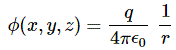
Feynman’s 28th Lecture in his series on electromagnetism is one of the more interesting but, at the same time, it’s one of the few Lectures that is clearly (out)dated. In essence, it talks about the difficulties involved in applying Maxwell’s equations to the elementary charges themselves, i.e. the electron and the proton. We already signaled some of these problems in previous posts. For example, in our post on the energy in electrostatic fields, we showed how our formulas for the field energy and/or the potential of a charge blow up when we use it to calculate the energy we’d need to assemble a point charge. What comes out is infinity: ∞. So our formulas tell us we’d need an infinite amount of energy to assemble a point charge.
Well… That’s no surprise, is it? The idea itself is impossible: how can one have a finite amount of charge in something that’s infinitely small? Something that has no size whatsoever? It’s pretty obvious we get some division by zero there. 🙂 The mathematical approach is often inconsistent. Indeed, a lot of blah-blah in physics is obviously just about applying formulas to situations that are clearly not within the relevant area of application of the formula. So that’s why I went through the trouble (in my previous post, that is) of explaining you how we get these energy and potential formulas, and that’s by bringing charges (note the plural) together. Now, we may assume these charges are point charges, but that assumption is not so essential. What I tried to say when being so explicit was the following: yes, a charge causes a field, but the idea of a potential makes sense only when we’re thinking of placing some other charge in that field. So point charges with ‘infinite energy’ should not be a problem. Feynman admits as much when he writes:
“If the energy can’t get out, but must stay there forever, is there any real difficulty with an infinite energy? Of course, a quantity that comes out infinite may be annoying, but what really matters is only whether there are any observable physical effects.”
So… Well… Let’s see. There’s another, more interesting, way to look at an electron: let’s have a look at the field it creates. A electron – stationary or moving – will create a field in Maxwell’s world, which we know inside out now. So let’s just calculate it. In fact, Feynman calculates it for the unit charge (+1), so that’s a positron. It eases the analysis because we don’t have to drag any minus sign along. So how does it work? Well…
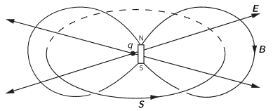
We’ll have an energy flux density vector – i.e. the Poynting vector S – as well as a momentum density vector g all over space. Both are related through the g = S/c2 equation which, as I explained in my previous post, is probably best written as cg = S/c, because we’ve got units then, on both sides, that we can readily understand, like N/m2 (so that’s force per unit area) or J/m3 (so that’s energy per unit volume). On the other hand, we’ll need something that’s written as a function of the velocity of our positron, so that’s v, and so it’s probably best to just calculate g, the momentum, which is measured in N·s or kg·(m/s2)·s (both are equivalent units for the momentum p = mv, indeed) per unit volume (so we need to add a 1/ m3 to the unit). So we’ll have some integral all over space, but I won’t bother you with it. Why not? Well… Feynman uses a rather particular volume element to solve the integral, and so I want you to focus on the solution. The geometry of the situation, and the solution for g, i.e. the momentum of the field per unit volume, is what matters here.
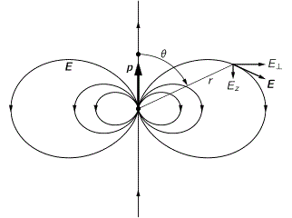
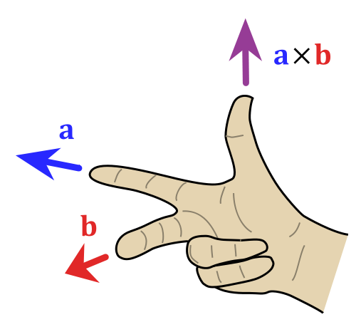
So let’s look at that geometry. It’s depicted below. We’ve got a radial electric field—a Coulomb field really, because our charge is moving at a non-relativistic speed, so v << c and we can approximate with a Coulomb field indeed. Maxwell’s equations imply that B = v×E/c2, so g = ε0E×B is what it is in the illustration below. Note that we’d have to reverse the direction of both E and B for an electron (because it’s negative), but g would be the same. It is directed obliquely toward the line of motion and its magnitude is g = (ε0v/c2)·E2·sinθ. Don’t worry about it: Feynman integrates this thing for you. 🙂 It’s not that difficult, but still… To solve it, he uses the fact that the fields are symmetric about the line of motion, which is indicated by the little arrow around the v-axis, with the Φ symbol next to it (it symbolizes the potential). [The ‘rather particular volume element’ is a ring around the v-axis, and it’s because of this symmetry that Feynman picks the ring. Feynman’s Lectures are not only great to learn physics: they’re a treasure drove of mathematical tricks too. :-)]

As said, I don’t want to bother you with the technicalities of the integral here. This is the result:
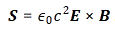
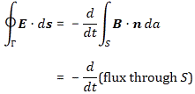
What does this say? It says that the momentum of the field – i.e. the electromagnetic momentum, integrated over all of space – is proportional to the velocity v of our charge. That makes sense: when v = 0, we’ll have an electrostatic field all over space and, hence, some inertia, but it’s only when we try to move our charge that Newton’s Law comes into play: then we’ll need some force to overcome that inertia. It all works through the Poynting formula: S = E×B/μ0. If nothing’s moving, then B = 0, and so we’ll have some E and, therefore, we’ll have field energy alright, but the energy flow will be zero. But when we move the charge, we’re moving the field, and so then B ≠ 0 and so it’s through B that the E in our S equation start kicking in. Does that make sense? Think about it: it’s good to try to visualize things in your mind. 🙂
The constants in the proportionality constant (2e2)/(3ac2) of our p ∼ v formula above are:
- e2 = qe2/(4πε0), with qe the electron charge (without the minus sign) and ε0 our ubiquitous electric constant. [Note that, unlike Feynman, I prefer to not write e in italics, so as to not confuse it with Euler’s number e ≈ 2.71828 etc. However, I know I am not always consistent in my notation.
 We don’t need Euler’s number in this post, so e or e is always an expression for the electron charge, not Euler’s number. Stupid remark, perhaps, but I don’t want you to be confused.]
 - a is the radius of our charge—see we got away from the idea of a point charge? 🙂
- c2 is just c2, i.e. our weird constant (the square of the speed of light) which seems to connect everything to everything. Indeed, think about stuff like this: S/g = c2 = 1/(ε0μ0).
Now, p = mv, so that formula for p basically says that our elementary charge (as mentioned, g is the same for a positron or an electron: E and B will be reversed, but g is not) has an electromagnetic mass melec equal to:
That’s an amazing result. We don’t need to give our electron any rest mass: just its charge and its movement will do! Super! So we don’t need any Higgs fields here! 🙂 The electromagnetic field will do!
Well… Maybe. Let’s explore what we’ve got here.
First, let’s compare that radius a in our formula to what’s found in experiments. Huh? Did someone ever try to measure the electron radius? Of course. There are all these scattering experiments in which electrons get fired at atoms. They can fly through or, else, hit something. Therefore, one can some statistical analysis and determine what is referred to as a cross-section. A cross-section is denoted by the same symbol as the standard deviation: σ (sigma). In any case… So there’s something that’s referred to as the classical electron radius, and it’s equal to the so-called Thomsom scattering length. Thomson scattering, as opposed to Compton scattering, is elastic scattering, so it preserves kinetic energy (unlike Compton scattering, where energy gets absorbed and changes frequencies). So… Well… I won’t go into too much detail but, yes, this is the electron radius we need. [I am saying this rather explicitly because there are two other numbers around: the so-called Bohr radius and, as you might imagine, the Compton scattering cross-section.]
The Thomson scattering length is 2.82 femtometer (so that’s 2.82×10⁻¹⁵ m), more or less that is :-), and it’s usually related to the observed electron mass me through the fine-structure constant α. In fact, using Planck units, we can write: re·me= α, which is an amazing formula but, unfortunately, I can’t dwell on it here. Using ordinary m, s, C and what have you units, we can write re as:

That’s good, because if we equate me and melec and switch melec and a in our formula for melec, we get:
So, frankly, we’re spot on! Well… Almost. The two numbers differ by 1/3. But who cares about a 1/3 factor indeed? We’re talking rather fuzzy stuff here – scattering cross-sections and standard deviations and all that – so… Yes. Well done! Our theory works!
Well… Maybe. Physicists don’t think so. They think the 1/3 factor is an issue. It’s sad because it really makes a lot of sense. In fact, the Dutch physicist Hendrik Lorentz – whom we know so well by now 🙂 – had also worked out that, because of the length contraction effect, our spherical charge would contract into an ellipsoid and… Well… He worked it all out, and it was not a problem: he found that the momentum was altered by the factor (1−v2/c2)−1/2, so that’s the ubiquitous Lorentz factor γ! He got this formula in the 1890s already, so that’s long before the theory of relativity had been developed. So, many years before Planck and Einstein would come up with their stuff, Hendrik Antoon Lorentz had the correct formulas already: the mass, or everything really, all should vary with that γ-factor. 🙂
Why bother about the 1/3 factor? [I should note it’s actually referred to as the 4/3 problem in physics.] Well… The critics do have a point: if we assume that (a) an electron is not a point charge – so if we allow it to have some radius a – and (b) that Maxwell’s Laws apply, then we should go all the way. The energy that’s needed to assemble an electron should then, effectively, be the same as the value we’d get out of those field energy formulas. So what do we get when we apply those formulas? Well… Let me quickly copy Feynman as he does the calculation for an electron, not looking at it as a point particle, but as a tiny shell of charge, i.e. a sphere with all charge sitting on the surface:
Let me enlarge the formula:
Now, if we combine that with our formula for melec above, then we get:
So that formula does not respect Einstein’s universal mass-energy equivalence formula E = mc2. Now, you will agree that we really want Einstein’s mass-energy equivalence relation to be respected by all, so our electron should respect it too. 🙂 So, yes, we’ve got a problem here, and it’s referred to as the 4/3 problem (yes, the ratio got turned around).
Now, you may think it got solved in the meanwhile. Well… No. It’s still a bit of a puzzle today, and the current-day explanation is not really different from what the French scientist Henri Poincaré proposed as a ‘solution’ to the problem back in the 1890s. He basically told Lorentz the following: “If the electron is some little ball of charge, then it should explode because of the repulsive forces inside. So there should be some binding forces there, and so that energy explains the ‘missing mass’ of the electron.” So these forces are effectively being referred to as Poincaré stresses, and the non-electromagnetic energy that’s associated with them – which, of course, has to be equal to 1/3 of the electromagnetic energy (I am sure you see why) 🙂 – adds to the total energy and all is alright now. We get:
U = mc2 = (melec + mPoincaré)c2
So… Yes… Pretty ad hoc. Worse, according to the Wikipedia article on electromagnetic mass, that’s still where we are. And, no, don’t read Feynman’s overview of all of the theories that were around then (so that’s in the 1960s, or earlier). As I said, it’s the one Lecture you don’t want to waste time on. So I won’t do that either.
In fact, let me try to do something else here, and that’s to de-construct the whole argument really. 🙂 Before I do so, let me highlight the essence of what was written above. It’s quite amazing really. Think of it: we say that the mass of an electron – i.e. its inertia, or the proportionality factor in Newton’s F = m·a law of motion – is the energy in the electric and magnetic field it causes. So the electron itself is just a hook for the force law, so to say. There’s nothing there, except for the charge causing the field. But so its mass is everywhere and, hence, nowhere really. Well… I should correct that: the field strength falls of as 1/r2 and, hence, the energy flow and momentum density that’s associated with it, falls of as 1/r4, so it falls of very rapidly and so the bulk of the energy is pretty near the charge. 🙂
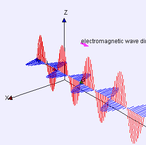
[Note: You’ll remember that the field that’s associated with electromagnetic radiation falls of as 1/r, not as 1/r2, which is why there is an energy flux there which is never lost, which can travel independently through space. It’s not the same here, so don’t get confused.]
So that’s something to note: the melec = (2c−2/3)·(e2/a) has the radius a in it, but that radius is only the hook, so to say. That’s fine, because it is not inconsistent with the idea of the Thomson scattering cross-section, which is the area that one can hit. Now, you’ll wonder how one can hit an electron: you can readily imagine an electron beam aimed at nuclei, but how would one hit electrons? Well… You can shoot photons at them, and see if they bounce back elastically or non-elastically. The cross-section area that bounces them off elastically must be pretty ‘hard’, and the cross-section that deflects them non-elastically somewhat less so. 🙂
OK… But… Yes? Hey! How did we get that electron radius in that formula?
Good question! Brilliant, in fact! You’re right: it’s here that the whole argument falls apart really. We did a substitution. That radius a is the radius of a spherical shell of charge with an energy that’s equal to Uelec = (1/2)·(e2/a), so there’s another way of stating the inconsistency: the equivalent energy of melec = (2c−2/3)·(e2)/a) is equal to E = melec·c2 = (2/3)·(e2/a) and that’s not the same as Uelec = (1/2)·(e2/a). If we take the ratio of Uelec and melec·c2 =, we get the same factor: (1/2)/(2/3) = 3/4. But… Your question is superb! Look at it: putting it the way we put it reveals the inconsistency in the whole argument. We’re mixing two things here:
- We first calculate the momentum density, and the momentum, that’s caused by the unit charge, so we get some energy which I’ll denote as Eelec = melec·c2
- Now, we then assume this energy must be equal to the energy that’s needed to assemble the unit charge from an infinite number of infinitesimally small charges, thereby also assuming the unit charge is a uniformly charged sphere of charge with radius a.
- We then use this radius a to simplify our formula for Eelec = melec·c2
Now that is not kosher, really! First, it’s (a) a lot of assumptions, both implicit as well as explicit, and then (b) it’s, quite simply, not a legit mathematical procedure: calculating the energy in the field, or calculating the energy we need to assemble a uniformly charged sphere of radius a are two very different things.
Well… Let me put it differently. We’re using the same laws – it’s all Maxwell’s equations, really – but we should be clear about what we’re doing with them, and those two things are very different. The legitimate conclusion must be that our a is wrong. In other words, we should not assume that our electron is spherical shell of charge. So then what? Well… We could easily imagine something else, like a uniform or even a non-uniformly charged sphere. Indeed, if we’re just filling empty space with infinitesimally small charge ‘elements’, then we may want to think the density at the ‘center’ will be much higher, like what’s going on when planets form: the density of the inner core of our own planet Earth is more than four times the density of its surface material. [OK. Perhaps not very relevant here, but you get the idea.] Or, conversely, taking into account Poincaré’s objection, we may want to think all of the charge will be on the surface, just like on a perfect conductor, where all charge is surface charge!
Note that the field outside of a uniformly charged sphere and the field of a spherical shell of charge is exactly the same, so we would not find a different number for Eelec = melec·c2, but we surely would find a different number for Uelec. You may want to look up some formulas here: you’ll find that the energy of a uniformly distributed sphere of charge (so we do not assume that all of the charge sits on the surface here) is equal to (3/5)·(e2/a). So we’d already have much less of a problem, because the 3/4 factor in the Uelec = (3/4)·melec·c2 becomes a (5/3)·(2/3) = 10/9 factor. So now we have a discrepancy of some 10% only. 🙂
You’ll say: 10% is 10%. It’s huge in physics, as it’s supposed to be an exact science. Well… It is and it isn’t. Do you realize we haven’t even started to talk about stuff like spin? Indeed, in modern physics, we think of electrons as something that also spins around one or the other axis, so there’s energy there too, and we didn’t include that in our analysis.
In short, Feynman’s approach here is disappointing. Naive even, but then… Well… Who knows? Perhaps he didn’t do this Lecture himself. Perhaps it’s just an assistant or so. In fact, I should wonder why there’s still physicists wasting time on this! I should also note that naively comparing that a radius with the classical electron radius also makes little or no sense. Unlike what you’d expect, the classical electron radius re and the Thomson scattering cross-section σe are not related like you might think they are, i.e. like σe = π·re2 or σe = π·(re/2)2 or σe = re2 or σe = π·(2·re)2 or whatever circular surface calculation rule that might make sense here. No. The Thomson scattering cross-section is equal to:
σe = (8π/3)·re2 = (2π/3)·(2·re)2 = (2/3)·π·(2·re)2 ≈ 66.5×10⁻³⁰ m2 = 66.5 (fm)2
Why? I am not sure. I must assume it’s got to do with the standard deviation and all that. The point is, we’ve got a 2/3 factor here too, so do we have a problem really? I mean… The a we got was equal to a = (2/3)·re, wasn’t it? It was. But, unfortunately, it doesn’t mean anything. It’s just a coincidence. In fact, looking at the Thomson scattering cross-section, instead of the Thomson scattering radius, makes the ‘problem’ a little bit worse. Indeed, applying the π·r2 rule for a circular surface, we get that the radius would be equal to (8/3)1/2·re ≈ 1.633·re, so we get something that’s much larger rather than something that’s smaller here.
In any case, it doesn’t matter. The point is: this kind of comparisons should not be taken too seriously. Indeed, when everything is said and done, we’re comparing three very different things here:
- The radius that’s associated with the energy that’s needed to assemble our electron from infinitesimally small charges, and so that’s based on Coulomb’s law and the model we use for our electron: is it a shell or a sphere of charge? If it’s a sphere, do we want to think of it as something that’s of uniform of non-uniform density.
- The second radius is associated with the field of an electron, which we calculate using Poynting’s formula for the energy flow and/or the momentum density. So that’s not about the internal structure of the electron but, of course, it would be nice if we could find some model of an electron that matches this radius.
- Finally, there’s the radius that’s associated with elastic scattering, which is also referred to as hard scattering because it’s like the collision of two hard spheres indeed. But so that’s some value that has to be established experimentally and so it involves judicious choices because there’s probabilities and standard deviations involved.
So should we worry about the gaps between these three different concepts? In my humble opinion: no. Why? Because they’re all damn close and so we’re actually talking about the same thing. I mean: isn’t terrific that we’ve got a model that brings the first and the second radius together with a difference of 10% only? As far as I am concerned, that shows the theory works. So what Feynman’s doing in that (in)famous chapter is some kind of ‘dimensional analysis’ which confirms rather than invalidates classical electromagnetic theory. So it shows classical theory’s strength, rather than its weakness. It actually shows our formula do work where we wouldn’t expect them to work. 🙂
The thing is: when looking at the behavior of electrons themselves, we’ll need a different conceptual framework altogether. I am talking quantum mechanics here. Indeed, we’ll encounter other anomalies than the ones we presented above. There’s the issue of the anomalous magnetic moment of electrons, for example. Indeed, as I mentioned above, we’ll also want to think as electrons as spinning around their own axis, and so that implies some circulation of E that will generate a permanent magnetic dipole moment… […] OK, just think of some magnetic field if you don’t have a clue what I am saying here (but then you should check out my post on it). […] The point is: here too, the so-called ‘classical result’, so that’s its theoretical value, will differ from the experimentally measured value. Now, the difference here will be 0.0011614, so that’s about 0.1%, i.e. 100 times smaller than my 10%. 🙂
Personally, I think that’s not so bad. 🙂 But then physicists need to stay in business, of course. So, yes, it is a problem. 🙂
Post scriptum on the math versus the physics
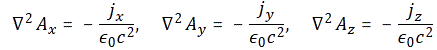
The key to the calculation of the energy that goes into assembling a charge was the following integral:
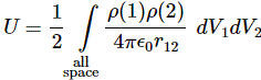
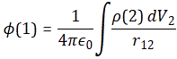
This is a double integral which we simplified in two stages, so we’re looking at an integral within an integral really, but we can substitute the integral over the ρ(2)·dV2 product by the formula we got for the potential, so we write that as Φ(1), and so the integral above becomes:
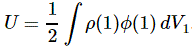 Now, this integral integrates the ρ(1)·Φ(1)·dV1 product over all of space, so that’s over all points in space, and so we just dropped the index and wrote the whole thing as the integral of ρ·Φ·dV over all of space:

We then established that this integral was mathematically equivalent to the following equation:
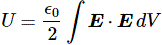
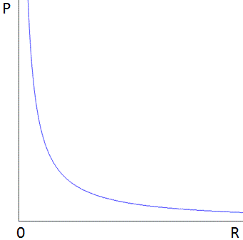
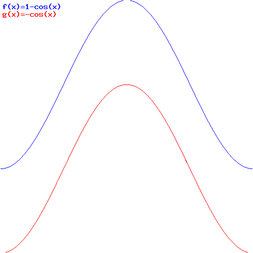
So this integral is actually quite simple: it just integrates E•E = E2 over all of space. The illustration below shows E as a function of the distance r for a sphere of radius R filled uniformly with charge.
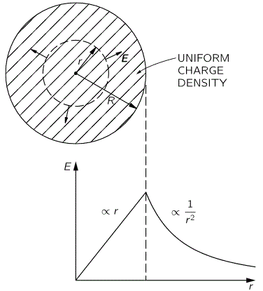
So the field (E) goes as r for r ≤ R and as 1/r2 for r ≥ R. So, for r ≥ R, the integral will have (1/r2)2 = 1/r4 in it. Now, you know that the integral of some function is the surface under the graph of that function. Look at the 1/r4 function below: it blows up between 1 and 0. That’s where the problem is: there needs to be some kind of cut-off, because that integral will effectively blow up when the radius of our little sphere of charge gets ‘too small’. So that makes it clear why it doesn’t make sense to use this formula to try to calculate the energy of a point charge. It just doesn’t make sense to do that.

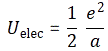
What’s ‘too small’? Let’s look at the formula we got for our electron as a spherical shell of charge:
So we’ve got an even simpler formula here: it’s just a 1/r relation. Why is that? Well… It’s just the way the math turns it out. I copied the detail of Feynman’s calculation above, so you can double-check it. It’s quite wonderful, really. We have a very simple inversely proportional relationship between the radius of our electron and its energy as a sphere of charge. We could write it as:
Uelect = α/a , with α = e2/2
But – Hey! Wait a minute! We’ve seen something like this before, haven’t we? We did. We did when we were discussing the wonderful properties of that magical number, the fine-structure constant, which we also denoted by α. 🙂 However, because we used α already, I’ll denote the fine-structure constant as αe here, so you don’t get confused. As you can see, the fine-structure constant links all of the fundamental properties of the electron: its charge, its radius, its distance to the nucleus (i.e. the Bohr radius), its velocity, and its mass (and, hence, its energy). So, at this stage of the argument, α can be anything, and αe cannot, of course. It’s just that magical number out there, which relates everything to everything: it’s the God-given number we don’t understand. 🙂 Having said that, it seems like we’re going to get some understanding here because we know that, one the many expressions involving αe was the following one:
me = αe/re
This says that the mass of the electron is equal to the ratio of the fine-structure constant and the electron radius. [Note that we express everything in natural units here, so that’s Planck units. For the detail of the conversion, please see the relevant section on that in my one of my posts on this and other stuff.] Now, mass is equivalent to energy, of course: it’s just a matter of units, so we can equate me with Ee (this amounts to expressing the energy of the electron in a kg unit—bit weird, but OK) and so we get:
Ee = αe/re
So there we have: the fine-structure constant αe is Nature’s ‘cut-off’ factor, so to speak. Why? Only God knows. 🙂 But it’s now (fairly) easy to see why all the relations involving αe are what they are. For example, we also know that αe is the square of the electron charge expressed in Planck units, so we have:
α = eP2 and, therefore, Ee = eP2/re
Now, you can check for yourself: it’s just a matter of re-expressing everything in standard SI units, and relating eP2 to e2, and it should all work: you should get the Uelect = (1/2)·e2/a expression. So… Well… At least this takes some of the magic out the fine-structure constant. It’s still a wonderful thing, but so you see that the fundamental relationship between (a) the energy (and, hence, the mass), (b) the radius and (c) the charge of an electron is not something God-given. What’s God-given are Maxwell’s equations, and so the Ee = αe/re = eP2/re is just one of the many wonderful things that you can get out of them. 🙂
Some content on this page was disabled on June 16, 2020 as a result of a DMCA takedown notice from The California Institute of Technology. You can learn more about the DMCA here:
https://wordpress.com/support/copyright-and-the-dmca/
Some content on this page was disabled on June 16, 2020 as a result of a DMCA takedown notice from The California Institute of Technology. You can learn more about the DMCA here:https://wordpress.com/support/copyright-and-the-dmca/
Some content on this page was disabled on June 16, 2020 as a result of a DMCA takedown notice from The California Institute of Technology. You can learn more about the DMCA here:https://wordpress.com/support/copyright-and-the-dmca/
Some content on this page was disabled on June 16, 2020 as a result of a DMCA takedown notice from The California Institute of Technology. You can learn more about the DMCA here:https://wordpress.com/support/copyright-and-the-dmca/
Some content on this page was disabled on June 16, 2020 as a result of a DMCA takedown notice from The California Institute of Technology. You can learn more about the DMCA here:https://wordpress.com/support/copyright-and-the-dmca/
Some content on this page was disabled on June 17, 2020 as a result of a DMCA takedown notice from Michael A. Gottlieb, Rudolf Pfeiffer, and The California Institute of Technology. You can learn more about the DMCA here:


 with
with 

