Ouff ! This title is quite a mouthful, isn’t it? 🙂 So… What’s the topic of the day? Well… In our previous posts, we developed a few key ideas in regard to a possible physical interpretation of the (elementary) wavefunction. It’s been an interesting excursion, and I summarized it in another pre-publication paper on the open arXiv.org site.
In my humble view, one of the toughest issues to deal with when thinking about geometric (or physical) interpretations of the wavefunction is the fact that a wavefunction does not seem to obey the classical 360° symmetry in space. In this post, I want to muse a bit about this and show that… Well… It does and it doesn’t. It’s got to do with what happens when you change from one representational base (or representation, tout court) to another which is… Well… Like changing the reference frame but, at the same time, it is also more than just a change of the reference frame—and so that explains the weird stuff (like that 720° symmetry of the amplitudes for spin-1/2 particles, for example).
I should warn you before you start reading: I’ll basically just pick up some statements from my paper (and previous posts) and develop some more thoughts on them. As a result, this post may not be very well structured. Hence, you may want to read the mentioned paper first.
The reality of directions
Huh? The reality of directions? Yes. I warned you. This post may cause brain damage. 🙂 The whole argument revolves around a thought experiment—but one whose results have been verified in zillions of experiments in university student labs so… Well… We do not doubt the results and, therefore, we do not doubt the basic mathematical results: we just want to try to understand them better.
So what is the set-up? Well… In the illustration below (Feynman, III, 6-3), Feynman compares the physics of two situations involving rather special beam splitters. Feynman calls them modified or ‘improved’ Stern-Gerlach apparatuses. The apparatus basically splits and then re-combines the two new beams along the z-axis. It is also possible to block one of the beams, so we filter out only particles with their spin up or, alternatively, with their spin down. Spin (or angular momentum or the magnetic moment) as measured along the z-axis, of course—I should immediately add: we’re talking the z-axis of the apparatus here.
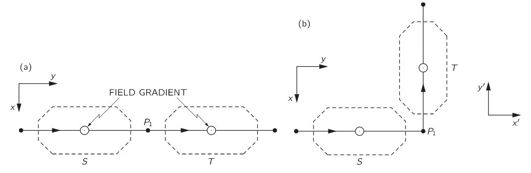
The two situations involve a different relative orientation of the apparatuses: in (a), the angle is 0°, while in (b) we have a (right-handed) rotation of 90° about the z-axis. He then proves—using geometry and logic only—that the probabilities and, therefore, the magnitudes of the amplitudes (denoted by C+ and C− and C’+ and C’− in the S and T representation respectively) must be the same, but the amplitudes must have different phases, noting—in his typical style, mixing academic and colloquial language—that “there must be some way for a particle to tell that it has turned a corner in (b).”
The various interpretations of what actually happens here may shed some light on the heated discussions on the reality of the wavefunction—and of quantum states. In fact, I should note that Feynman’s argument revolves around quantum states. To be precise, the analysis is focused on two-state systems only, and the wavefunction—which captures a continuum of possible states, so to speak—is introduced only later. However, we may look at the amplitude for a particle to be in the up– or down-state as a wavefunction and, therefore (but do note that’s my humble opinion once more), the analysis is actually not all that different.
We know, from theory and experiment, that the amplitudes are different. For example, for the given difference in the relative orientation of the two apparatuses (90°), we know that the amplitudes are given by C’+ = ei∙φ/2∙C+ = e i∙π/4∙C+ and C’− = e−i∙φ/2∙C+ = e− i∙π/4∙C− respectively (the amplitude to go from the down to the up state, or vice versa, is zero). Hence, yes, we—not the particle, Mr. Feynman!—know that, in (b), the electron has, effectively, turned a corner.
The more subtle question here is the following: is the reality of the particle in the two setups the same? Feynman, of course, stays away from such philosophical question. He just notes that, while “(a) and (b) are different”, “the probabilities are the same”. He refrains from making any statement on the particle itself: is or is it not the same? The common sense answer is obvious: of course, it is! The particle is the same, right? In (b), it just took a turn—so it is just going in some other direction. That’s all.
However, common sense is seldom a good guide when thinking about quantum-mechanical realities. Also, from a more philosophical point of view, one may argue that the reality of the particle is not the same: something might—or must—have happened to the electron because, when everything is said and done, the particle did take a turn in (b). It did not in (a). [Note that the difference between ‘might’ and ‘must’ in the previous phrase may well sum up the difference between a deterministic and a non-deterministic world view but… Well… This discussion is going to be way too philosophical already, so let’s refrain from inserting new language here.]
Let us think this through. The (a) and (b) set-up are, obviously, different but… Wait a minute… Nothing is obvious in quantum mechanics, right? How can we experimentally confirm that they are different?
Huh? I must be joking, right? You can see they are different, right? No. I am not joking. In physics, two things are different if we get different measurement results. [That’s a bit of a simplified view of the ontological point of view of mainstream physicists, but you will have to admit I am not far off.] So… Well… We can’t see those amplitudes and so… Well… If we measure the same thing—same probabilities, remember?—why are they different? Think of this: if we look at the two beam splitters as one single tube (an ST tube, we might say), then all we did in (b) was bend the tube. Pursuing the logic that says our particle is still the same even when it takes a turn, we could say the tube is still the same, despite us having wrenched it over a 90° corner.
Now, I am sure you think I’ve just gone nuts, but just try to stick with me a little bit longer. Feynman actually acknowledges the same: we need to experimentally prove (a) and (b) are different. He does so by getting a third apparatus in (U), as shown below, whose relative orientation to T is the same in both (a) and (b), so there is no difference there.

Now, the axis of U is not the z-axis: it is the x-axis in (a), and the y-axis in (b). So what? Well… I will quote Feynman here—not (only) because his words are more important than mine but also because every word matters here:
“The two apparatuses in (a) and (b) are, in fact, different, as we can see in the following way. Suppose that we put an apparatus in front of S which produces a pure +x state. Such particles would be split into +z and −z into beams in S, but the two beams would be recombined to give a +x state again at P1—the exit of S. The same thing happens again in T. If we follow T by a third apparatus U, whose axis is in the +x direction and, as shown in (a), all the particles would go into the + beam of U. Now imagine what happens if T and U are swung around together by 90° to the positions shown in (b). Again, the T apparatus puts out just what it takes in, so the particles that enter U are in a +x state with respect to S, which is different. By symmetry, we would now expect only one-half of the particles to get through.”
I should note that (b) shows the U apparatus wide open so… Well… I must assume that’s a mistake (and should alert the current editors of the Lectures to it): Feynman’s narrative tells us we should also imagine it with the minus channel shut. In that case, it should, effectively, filter approximately half of the particles out, while they all get through in (a). So that’s a measurement result which shows the direction, as we see it, makes a difference.
Now, Feynman would be very angry with me—because, as mentioned, he hates philosophers—but I’d say: this experiment proves that a direction is something real. Of course, the next philosophical question then is: what is a direction? I could answer this by pointing to the experiment above: a direction is something that alters the probabilities between the STU tube as set up in (a) versus the STU tube in (b). In fact—but, I admit, that would be pretty ridiculous—we could use the varying probabilities as we wrench this tube over varying angles to define an angle! But… Well… While that’s a perfectly logical argument, I agree it doesn’t sound very sensical.
OK. Next step. What follows may cause brain damage. 🙂 Please abandon all pre-conceived notions and definitions for a while and think through the following logic.
You know this stuff is about transformations of amplitudes (or wavefunctions), right? [And you also want to hear about those special 720° symmetry, right? No worries. We’ll get there.] So the questions all revolve around this: what happens to amplitudes (or the wavefunction) when we go from one reference frame—or representation, as it’s referred to in quantum mechanics—to another?
Well… I should immediately correct myself here: a reference frame and a representation are two different things. They are related but… Well… Different… Quite different. Not same-same but different. 🙂 I’ll explain why later. Let’s go for it.
Before talking representations, let us first think about what we really mean by changing the reference frame. To change it, we first need to answer the question: what is our reference frame? It is a mathematical notion, of course, but then it is also more than that: it is our reference frame. We use it to make measurements. That’s obvious, you’ll say, but let me make a more formal statement here:
The reference frame is given by (1) the geometry (or the shape, if that sounds easier to you) of the measurement apparatus (so that’s the experimental set-up) here) and (2) our perspective of it.
If we would want to sound academic, we might refer to Kant and other philosophers here, who told us—230 years ago—that the mathematical idea of a three-dimensional reference frame is grounded in our intuitive notions of up and down, and left and right. [If you doubt this, think about the necessity of the various right-hand rules and conventions that we cannot do without in math, and in physics.] But so we do not want to sound academic. Let us be practical. Just think about the following. The apparatus gives us two directions:
(1) The up direction, which we associate with the positive direction of the z-axis, and
(2) the direction of travel of our particle, which we associate with the positive direction of the y-axis.
Now, if we have two axes, then the third axis (the x-axis) will be given by the right-hand rule, right? So we may say the apparatus gives us the reference frame. Full stop. So… Well… Everything is relative? Is this reference frame relative? Are directions relative? That’s what you’ve been told, but think about this: relative to what? Here is where the object meets the subject. What’s relative? What’s absolute? Frankly, I’ve started to think that, in this particular situation, we should, perhaps, not use these two terms. I am not saying that our observation of what physically happens here gives these two directions any absolute character but… Well… You will have to admit they are more than just some mathematical construct: when everything is said and done, we will have to admit that these two directions are real. because… Well… They’re part of the reality that we are observing, right? And the third one… Well… That’s given by our perspective—by our right-hand rule, which is… Well… Our right-hand rule.
Of course, now you’ll say: if you think that ‘relative’ and ‘absolute’ are ambiguous terms and that we, therefore, may want to avoid them a bit more, then ‘real’ and its opposite (unreal?) are ambiguous terms too, right? Well… Maybe. What language would you suggest? 🙂 Just stick to the story for a while. I am not done yet. So… Yes… What is their reality? Let’s think about that in the next section.
Perspectives, reference frames and symmetries
You’ve done some mental exercises already as you’ve been working your way through the previous section, but you’ll need to do plenty more. In fact, they may become physical exercise too: when I first thought about these things (symmetries and, more importantly, asymmetries in space), I found myself walking around the table with some asymmetrical everyday objects and papers with arrows and clocks and other stuff on it—effectively analyzing what right-hand screw, thumb or grip rules actually mean. 🙂
So… Well… I want you to distinguish—just for a while—between the notion of a reference frame (think of the x–y–z reference frame that comes with the apparatus) and your perspective on it. What’s our perspective on it? Well… You may be looking from the top, or from the side and, if from the side, from the left-hand side or the right-hand side—which, if you think about it, you can only define in terms of the various positive and negative directions of the various axes. 🙂 If you think this is getting ridiculous… Well… Don’t. Feynman himself doesn’t think this is ridiculous, because he starts his own “long and abstract side tour” on transformations with a very simple explanation of how the top and side view of the apparatus are related to the axes (i.e. the reference frame) that comes with it. You don’t believe me? This is the very first illustration of his Lecture on this:
 He uses it to explain the apparatus (which we don’t do here because you’re supposed to already know how these (modified or improved) Stern-Gerlach apparatuses work). So let’s continue this story. Suppose that we are looking in the positive y-direction—so that’s the direction in which our particle is moving—then we might imagine how it would look like when we would make a 180° turn and look at the situation from the other side, so to speak. We do not change the reference frame (i.e. the orientation) of the apparatus here: we just change our perspective on it. Instead of seeing particles going away from us, into the apparatus, we now see particles coming towards us, out of the apparatus.
What happens—but that’s not scientific language, of course—is that left becomes right, and right becomes left. Top still is top, and bottom is bottom. We are looking now in the negative y-direction, and the positive direction of the x-axis—which pointed right when we were looking in the positive y-direction—now points left. I see you nodding your head now—because you’ve heard about parity inversions, mirror symmetries and what have you—and I hear you say: “That’s the mirror world, right?”
No. It is not. I wrote about this in another post: the world in the mirror is the world in the mirror. We don’t get a mirror image of an object by going around it and looking at its back side. I can’t dwell too much on this (just check that post, and another one who talks about the same), but so don’t try to connect it to the discussions on symmetry-breaking and what have you. Just stick to this story, which is about transformations of amplitudes (or wavefunctions). [If you really want to know—but I know this sounds counterintuitive—the mirror world doesn’t really switch left for right. Your reflection doesn’t do a 180 degree turn: it is just reversed front to back, with no rotation at all. It’s only your brain which mentally adds (or subtracts) the 180 degree turn that you assume must have happened from the observed front to back reversal. So the left to right reversal is only apparent. It’s a common misconception, and… Well… I’ll let you figure this out yourself. I need to move on.] Just note the following:
- The xyz reference frame remains a valid right-handed reference frame. Of course it does: it comes with our beam splitter, and we can’t change its reality, right? We’re just looking at it from another angle. Our perspective on it has changed.
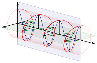
- However, if we think of the real and imaginary part of the wavefunction describing the electrons that are going through our apparatus as perpendicular oscillations (as shown below)—a cosine and sine function respectively—then our change in perspective might, effectively, mess up our convention for measuring angles.
I am not saying it does. Not now, at least. I am just saying it might. It depends on the plane of the oscillation, as I’ll explain in a few moments. Think of this: we measure angles counterclockwise, right? As shown below… But… Well… If the thing below would be some funny clock going backwards—you’ve surely seen them in a bar or so, right?—then… Well… If they’d be transparent, and you’d go around them, you’d see them as going… Yes… Clockwise. 🙂 [This should remind you of a discussion on real versus pseudo-vectors, or polar versus axial vectors, but… Well… We don’t want to complicate the story here.]

Now, if we would assume this clock represents something real—and, of course, I am thinking of the elementary wavefunction eiθ = cosθ + i·sinθ now—then… Well… Then it will look different when we go around it. When going around our backwards clock above and looking at it from… Well… The back, we’d describe it, naively, as… Well… Think! What’s your answer? Give me the formula! 🙂
[…]
We’d see it as e−iθ = cos(−θ) + i·sin(−θ) = cosθ − i·sinθ, right? The hand of our clock now goes clockwise, so that’s the opposite direction of our convention for measuring angles. Hence, instead of eiθ, we write e−iθ, right? So that’s the complex conjugate. So we’ve got a different image of the same thing here. Not good. Not good at all. ![]()
You’ll say: so what? We can fix this thing easily, right? You don’t need the convention for measuring angles or for the imaginary unit (i) here. This particle is moving, right? So if you’d want to look at the elementary wavefunction as some sort of circularly polarized beam (which, I admit, is very much what I would like to do, but its polarization is rather particular as I’ll explain in a minute), then you just need to define left- and right-handed angles as per the standard right-hand screw rule (illustrated below). To hell with the counterclockwise convention for measuring angles!

You are right. We could use the right-hand rule more consistently. We could, in fact, use it as an alternative convention for measuring angles: we could, effectively, measure them clockwise or counterclockwise depending on the direction of our particle. But… Well… The fact is: we don’t. We do not use that alternative convention when we talk about the wavefunction. Physicists do use the counterclockwise convention all of the time and just jot down these complex exponential functions and don’t realize that, if they are to represent something real, our perspective on the reference frame matters. To put it differently, the direction in which we are looking at things matters! Hence, the direction is not… Well… I am tempted to say… Not relative at all but then… Well… We wanted to avoid that term, right? 🙂
[…]
I guess that, by now, your brain may suffered from various short-circuits. If not, stick with me a while longer. Let us analyze how our wavefunction model might be impacted by this symmetry—or asymmetry, I should say.
The flywheel model of an electron
In our previous posts, we offered a model that interprets the real and the imaginary part of the wavefunction as oscillations which each carry half of the total energy of the particle. These oscillations are perpendicular to each other, and the interplay between both is how energy propagates through spacetime. Let us recap the fundamental premises:
- The dimension of the matter-wave field vector is force per unit mass (N/kg), as opposed to the force per unit charge (N/C) dimension of the electric field vector. This dimension is an acceleration (m/s2), which is the dimension of the gravitational field.
- We assume this gravitational disturbance causes our electron (or a charged mass in general) to move about some center, combining linear and circular motion. This interpretation reconciles the wave-particle duality: fields interfere but if, at the same time, they do drive a pointlike particle, then we understand why, as Feynman puts it, “when you do find the electron some place, the entire charge is there.” Of course, we cannot prove anything here, but our elegant yet simple derivation of the Compton radius of an electron is… Well… Just nice. 🙂
- Finally, and most importantly in the context of this discussion, we noted that, in light of the direction of the magnetic moment of an electron in an inhomogeneous magnetic field, the plane which circumscribes the circulatory motion of the electron should also comprise the direction of its linear motion. Hence, unlike an electromagnetic wave, the plane of the two-dimensional oscillation (so that’s the polarization plane, really) cannot be perpendicular to the direction of motion of our electron.
Let’s say some more about the latter point here. The illustrations below (one from Feynman, and the other is just open-source) show what we’re thinking of. The direction of the angular momentum (and the magnetic moment) of an electron—or, to be precise, its component as measured in the direction of the (inhomogeneous) magnetic field through which our electron is traveling—cannot be parallel to the direction of motion. On the contrary, it must be perpendicular to the direction of motion. In other words, if we imagine our electron as spinning around some center (see the illustration on the left-hand side), then the disk it circumscribes (i.e. the plane of the polarization) has to comprise the direction of motion.


Of course, we need to add another detail here. As my readers will know, we do not really have a precise direction of angular momentum in quantum physics. While there is no fully satisfactory explanation of this, the classical explanation—combined with the quantization hypothesis—goes a long way in explaining this: an object with an angular momentum J and a magnetic moment μ that is not exactly parallel to some magnetic field B, will not line up: it will precess—and, as mentioned, the quantization of angular momentum may well explain the rest. [Well… Maybe… We have detailed our attempts in this regard in various posts on this (just search for spin or angular momentum on this blog, and you’ll get a dozen posts or so), but these attempts are, admittedly, not fully satisfactory. Having said that, they do go a long way in relating angles to spin numbers.]
The thing is: we do assume our electron is spinning around. If we look from the up-direction only, then it will be spinning clockwise if its angular momentum is down (so its magnetic moment is up). Conversely, it will be spinning counterclockwise if its angular momentum is up. Let us take the up-state. So we have a top view of the apparatus, and we see something like this: I know you are laughing aloud now but think of your amusement as a nice reward for having stuck to the story so far. Thank you. 🙂 And, yes, do check it yourself by doing some drawings on your table or so, and then look at them from various directions as you walk around the table as—I am not ashamed to admit this—I did when thinking about this. So what do we get when we change the perspective? Let us walk around it, counterclockwise, let’s say, so we’re measuring our angle of rotation as some positive angle. Walking around it—in whatever direction, clockwise or counterclockwise—doesn’t change the counterclockwise direction of our… Well… That weird object that might—just might—represent an electron that has its spin up and that is traveling in the positive y-direction.
When we look in the direction of propagation (so that’s from left to right as you’re looking at this page), and we abstract away from its linear motion, then we could, vaguely, describe this by some wrenched eiθ = cosθ + i·sinθ function, right? The x- and y-axes of the apparatus may be used to measure the cosine and sine components respectively.
Let us keep looking from the top but walk around it, rotating ourselves over a 180° angle so we’re looking in the negative y-direction now. As I explained in one of those posts on symmetries, our mind will want to switch to a new reference frame: we’ll keep the z-axis (up is up, and down is down), but we’ll want the positive direction of the x-axis to… Well… Point right. And we’ll want the y-axis to point away, rather than towards us. In short, we have a transformation of the reference frame here: z’ = z, y’ = − y, and x’ = − x. Mind you, this is still a regular right-handed reference frame. [That’s the difference with a mirror image: a mirrored right-hand reference frame is no longer right-handed.] So, in our new reference frame, that we choose to coincide with our perspective, we will now describe the same thing as some −cosθ − i·sinθ = −eiθ function. Of course, −cosθ = cos(θ + π) and −sinθ = sin(θ + π) so we can write this as:
−cosθ − i·sinθ = cos(θ + π) + i·sinθ = ei·(θ+π) = eiπ·eiθ = −eiθ.
Sweet ! But… Well… First note this is not the complex conjugate: e−iθ = cosθ − i·sinθ ≠ −cosθ − i·sinθ = −eiθ. Why is that? Aren’t we looking at the same clock, but from the back? No. The plane of polarization is different. Our clock is more like those in Dali’s painting: it’s flat. 🙂 And, yes, let me lighten up the discussion with that painting here. 🙂 We need to have some fun while torturing our brain, right?

So, because we assume the plane of polarization is different, we get an −eiθ function instead of a e−iθ function.
Let us now think about the ei·(θ+π) function. It’s the same as −eiθ but… Well… We walked around the z-axis taking a full 180° turn, right? So that’s π in radians. So that’s the phase shift here. Hey! Try the following now. Go back and walk around the apparatus once more, but let the reference frame rotate with us, as shown below. So we start left and look in the direction of propagation, and then we start moving about the z-axis (which points out of this page, toward you, as you are looking at this), let’s say by some small angle α. So we rotate the reference frame about the z-axis by α and… Well… Of course, our ei·θ now becomes an our ei·(θ+α) function, right? We’ve just derived the transformation coefficient for a rotation about the z-axis, didn’t we? It’s equal to ei·α, right? We get the transformed wavefunction in the new reference frame by multiplying the old one by ei·α, right? It’s equal to ei·α·ei·θ = ei·(θ+α), right?
 Well…
Well…
[…]
No. The answer is: no. The transformation coefficient is not ei·α but ei·α/2. So we get an additional 1/2 factor in the phase shift.
Huh? Yes. That’s what it is: when we change the representation, by rotating our apparatus over some angle α about the z-axis, then we will, effectively, get a new wavefunction, which will differ from the old one by a phase shift that is equal to only half of the rotation angle only.
Huh? Yes. It’s even weirder than that. For a spin down electron, the transformation coefficient is e−i·α/2, so we get an additional minus sign in the argument.
Huh? Yes.
I know you are terribly disappointed, but that’s how it is. That’s what hampers an easy geometric interpretation of the wavefunction. Paraphrasing Feynman, I’d say that, somehow, our electron not only knows whether or not it has taken a turn, but it also knows whether or not it is moving away from us or, conversely, towards us.
[…]
But… Hey! Wait a minute! That’s it, right?
What? Well… That’s it! The electron doesn’t know whether it’s moving away or towards us. That’s nonsense. But… Well… It’s like this:
Our ei·α coefficient describes a rotation of the reference frame. In contrast, the ei·α/2 and e−i·α/2 coefficients describe what happens when we rotate the T apparatus! Now that is a very different proposition.
Right! You got it! Representations and reference frames are different things. Quite different, I’d say: representations are real, reference frames aren’t—but then you don’t like philosophical language, do you? 🙂 But think of it. When we just go about the z-axis, a full 180°, but we don’t touch that T-apparatus, we don’t change reality. When we were looking at the electron while standing left to the apparatus, we watched the electrons going in and moving away from us, and when we go about the z-axis, a full 180°, looking at it from the right-hand side, we see the electrons coming out, moving towards us. But it’s still the same reality. We simply change the reference frame—from xyz to x’y’z’ to be precise: we do not change the representation.
In contrast, when we rotate the T apparatus over a full 180°, our electron now goes in the opposite direction. And whether that’s away or towards us, that doesn’t matter: it was going in one direction while traveling through S, and now it goes in the opposite direction—relative to the direction it was going in S, that is.
So what happens, really, when we change the representation, rather than the reference frame? Well… Let’s think about that. 🙂
Quantum-mechanical weirdness?
The transformation matrix for the amplitude of a system to be in an up or down state (and, hence, presumably, for a wavefunction) for a rotation about the z-axis is the following one:
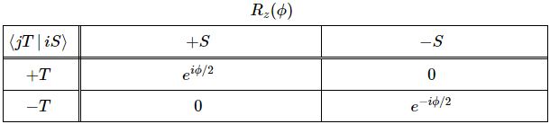
Feynman derives this matrix in a rather remarkable intellectual tour de force in the 6th of his Lectures on Quantum Mechanics. So that’s pretty early on. He’s actually worried about that himself, apparently, and warns his students that “This chapter is a rather long and abstract side tour, and it does not introduce any idea which we will not also come to by a different route in later chapters. You can, therefore, skip over it, and come back later if you are interested.”
Well… That’s how I approached it. I skipped it, and didn’t worry about those transformations for quite a while. But… Well… You can’t avoid them. In some weird way, they are at the heart of the weirdness of quantum mechanics itself. Let us re-visit his argument. Feynman immediately gets that the whole transformation issue here is just a matter of finding an easy formula for that phase shift. Why? He doesn’t tell us. Lesser mortals like us must just assume that’s how the instinct of a genius works, right? 🙂 So… Well… Because he knows—from experiment—that the coefficient is ei·α/2 instead of ei·α, he just says the phase shift—which he denotes by λ—must be some proportional to the angle of rotation—which he denotes by φ rather than α (so as to avoid confusion with the Euler angle α). So he writes:
λ = m·φ
Initially, he also tries the obvious thing: m should be one, right? So λ = φ, right? Well… No. It can’t be. Feynman shows why that can’t be the case by adding a third apparatus once again, as shown below.
Let me quote him here, as I can’t explain it any better:
“Suppose T is rotated by 360°; then, clearly, it is right back at zero degrees, and we should have C’+ = C+ and C’− = C− or, what is the same thing, ei·m·2π = 1. We get m = 1. [But no!] This argument is wrong! To see that it is, consider that T is rotated by 180°. If m were equal to 1, we would have C’+ = ei·πC+ = −C+ and C’− = e−i·πC− = −C−. [Feynman works with states here, instead of the wavefunction of the particle as a whole. I’ll come back to this.] However, this is just the original state all over again. Both amplitudes are just multiplied by −1 which gives back the original physical system. (It is again a case of a common phase change.) This means that if the angle between T and S is increased to 180°, the system would be indistinguishable from the zero-degree situation, and the particles would again go through the (+) state of the U apparatus. At 180°, though, the (+) state of the U apparatus is the (−x) state of the original S apparatus. So a (+x) state would become a (−x) state. But we have done nothing to change the original state; the answer is wrong. We cannot have m = 1. We must have the situation that a rotation by 360°, and no smaller angle reproduces the same physical state. This will happen if m = 1/2.”
The result, of course, is this weird 720° symmetry. While we get the same physics after a 360° rotation of the T apparatus, we do not get the same amplitudes. We get the opposite (complex) number: C’+ = ei·2π/2C+ = −C+ and C’− = e−i·2π/2C− = −C−. That’s OK, because… Well… It’s a common phase shift, so it’s just like changing the origin of time. Nothing more. Nothing less. Same physics. Same reality. But… Well… C’+ ≠ −C+ and C’− ≠ −C−, right? We only get our original amplitudes back if we rotate the T apparatus two times, so that’s by a full 720 degrees—as opposed to the 360° we’d expect.
Now, space is isotropic, right? So this 720° business doesn’t make sense, right?
Well… It does and it doesn’t. We shouldn’t dramatize the situation. What’s the actual difference between a complex number and its opposite? It’s like x or −x, or t and −t. I’ve said this a couple of times already again, and I’ll keep saying it many times more: Nature surely can’t be bothered by how we measure stuff, right? In the positive or the negative direction—that’s just our choice, right? Our convention. So… Well… It’s just like that −eiθ function we got when looking at the same experimental set-up from the other side: our eiθ and −eiθ functions did not describe a different reality. We just changed our perspective. The reference frame. As such, the reference frame isn’t real. The experimental set-up is. And—I know I will anger mainstream physicists with this—the representation is. Yes. Let me say it loud and clear here:
A different representation describes a different reality.
In contrast, a different perspective—or a different reference frame—does not.
Conventions
While you might have had a lot of trouble going through all of the weird stuff above, the point is: it is not all that weird. We can understand quantum mechanics. And in a fairly intuitive way, really. It’s just that… Well… I think some of the conventions in physics hamper such understanding. Well… Let me be precise: one convention in particular, really. It’s that convention for measuring angles. Indeed, Mr. Leonhard Euler, back in the 18th century, might well be “the master of us all” (as Laplace is supposed to have said) but… Well… He couldn’t foresee how his omnipresent formula—eiθ = cosθ + i·sinθ—would, one day, be used to represent something real: an electron, or any elementary particle, really. If he would have known, I am sure he would have noted what I am noting here: Nature can’t be bothered by our conventions. Hence, if eiθ represents something real, then e−iθ must also represent something real. [Coz I admire this genius so much, I can’t resist the temptation. Here’s his portrait. He looks kinda funny here, doesn’t he? :-)]

Frankly, he would probably have understood quantum-mechanical theory as easily and instinctively as Dirac, I think, and I am pretty sure he would have noted—and, if he would have known about circularly polarized waves, probably agreed to—that alternative convention for measuring angles: we could, effectively, measure angles clockwise or counterclockwise depending on the direction of our particle—as opposed to Euler’s ‘one-size-fits-all’ counterclockwise convention. But so we did not adopt that alternative convention because… Well… We want to keep honoring Euler, I guess. 🙂
So… Well… If we’re going to keep honoring Euler by sticking to that ‘one-size-fits-all’ counterclockwise convention, then I do believe that eiθ and e−iθ represent two different realities: spin up versus spin down.
Yes. In our geometric interpretation of the wavefunction, these are, effectively, two different spin directions. And… Well… These are real directions: we see something different when they go through a Stern-Gerlach apparatus. So it’s not just some convention to count things like 0, 1, 2, etcetera versus 0, −1, −2 etcetera. It’s the same story again: different but related mathematical notions are (often) related to different but related physical possibilities. So… Well… I think that’s what we’ve got here. Think of it. Mainstream quantum math treats all wavefunctions as right-handed but… Well… A particle with up spin is a different particle than one with down spin, right? And, again, Nature surely cannot be bothered about our convention of measuring phase angles clockwise or counterclockwise, right? So… Well… Kinda obvious, right? 🙂
Let me spell out my conclusions here:
1. The angular momentum can be positive or, alternatively, negative: J = +ħ/2 or −ħ/2. [Let me note that this is not obvious. Or less obvious than it seems, at first. In classical theory, you would expect an electron, or an atomic magnet, to line up with the field. Well… The Stern-Gerlach experiment shows they don’t: they keep their original orientation. Well… If the field is weak enough.]
2. Therefore, we would probably like to think that an actual particle—think of an electron, or whatever other particle you’d think of—comes in two variants: right-handed and left-handed. They will, therefore, either consist of (elementary) right-handed waves or, else, (elementary) left-handed waves. An elementary right-handed wave would be written as: ψ(θi) = eiθi = ai·(cosθi + i·sinθi). In contrast, an elementary left-handed wave would be written as: ψ(θi) = e−iθi = ai·(cosθi − i·sinθi). So that’s the complex conjugate.
So… Well… Yes, I think complex conjugates are not just some mathematical notion: I believe they represent something real. It’s the usual thing: Nature has shown us that (most) mathematical possibilities correspond to real physical situations so… Well… Here you go. It is really just like the left- or right-handed circular polarization of an electromagnetic wave: we can have both for the matter-wave too! [As for the differences—different polarization plane and dimensions and what have you—I’ve already summed those up, so I won’t repeat myself here.] The point is: if we have two different physical situations, we’ll want to have two different functions to describe it. Think of it like this: why would we have two—yes, I admit, two related—amplitudes to describe the up or down state of the same system, but only one wavefunction for it? You tell me.
[…]
Authors like me are looked down upon by the so-called professional class of physicists. The few who bothered to react to my attempts to make sense of Einstein’s basic intuition in regard to the nature of the wavefunction all said pretty much the same thing: “Whatever your geometric (or physical) interpretation of the wavefunction might be, it won’t be compatible with the isotropy of space. You cannot imagine an object with a 720° symmetry. That’s geometrically impossible.”
Well… Almost three years ago, I wrote the following on this blog: “As strange as it sounds, a spin-1/2 particle needs two full rotations (2×360°=720°) until it is again in the same state. Now, in regard to that particularity, you’ll often read something like: “There is nothing in our macroscopic world which has a symmetry like that.” Or, worse, “Common sense tells us that something like that cannot exist, that it simply is impossible.” [I won’t quote the site from which I took this quotes, because it is, in fact, the site of a very respectable research center!] Bollocks! The Wikipedia article on spin has this wonderful animation: look at how the spirals flip between clockwise and counterclockwise orientations, and note that it’s only after spinning a full 720 degrees that this ‘point’ returns to its original configuration after spinning a full 720 degrees.
So… Well… I am still pursuing my original dream which is… Well… Let me re-phrase what I wrote back in January 2015:
Yes, we can actually imagine spin-1/2 particles, and we actually do not need all that much imagination!
In fact, I am tempted to think that I’ve found a pretty good representation or… Well… A pretty good image, I should say, because… Well… A representation is something real, remember? 🙂
Post scriptum (10 December 2017): Our flywheel model of an electron makes sense, but also leaves many unanswered questions. The most obvious one question, perhaps, is: why the up and down state only?
I am not so worried about that question, even if I can’t answer it right away because… Well… Our apparatus—the way we measure reality—is set up to measure the angular momentum (or the magnetic moment, to be precise) in one direction only. If our electron is captured by some harmonic (or non-harmonic?) oscillation in multiple dimensions, then it should not be all that difficult to show its magnetic moment is going to align, somehow, in the same or, alternatively, the opposite direction of the magnetic field it is forced to travel through.
Of course, the analysis for the spin up situation (magnetic moment down) is quite peculiar: if our electron is a mini-magnet, why would it not line up with the magnetic field? We understand the precession of a spinning top in a gravitational field, but… Hey… It’s actually not that different. Try to imagine some spinning top on the ceiling. 🙂 I am sure we can work out the math. 🙂 The electron must be some gyroscope, really: it won’t change direction. In other words, its magnetic moment won’t line up. It will precess, and it can do so in two directions, depending on its state. 🙂 […] At least, that’s why my instinct tells me. I admit I need to work out the math to convince you. 🙂
The second question is more important. If we just rotate the reference frame over 360°, we see the same thing: some rotating object which we, vaguely, describe by some e+i·θ function—to be precise, I should say: by some Fourier sum of such functions—or, if the rotation is in the other direction, by some e−i·θ function (again, you should read: a Fourier sum of such functions). Now, the weird thing, as I tried to explain above is the following: if we rotate the object itself, over the same 360°, we get a different object: our ei·θ and e−i·θ function (again: think of a Fourier sum, so that’s a wave packet, really) becomes a −e±i·θ thing. We get a minus sign in front of it. So what happened here? What’s the difference, really?
Well… I don’t know. It’s very deep. If I do nothing, and you keep watching me while turning around me, for a full 360°, then you’ll end up where you were when you started and, importantly, you’ll see the same thing. Exactly the same thing: if I was an e+i·θ wave packet, I am still an an e+i·θ wave packet now. Or if I was an e−i·θ wave packet, then I am still an an e−i·θ wave packet now. Easy. Logical. Obvious, right?
But so now we try something different: I turn around, over a full 360° turn, and you stay where you are. When I am back where I was—looking at you again, so to speak—then… Well… I am not quite the same any more. Or… Well… Perhaps I am but you see me differently. If I was e+i·θ wave packet, then I’ve become a −e+i·θ wave packet now. Not hugely different but… Well… That minus sign matters, right? Or If I was wave packet built up from elementary a·e−i·θ waves, then I’ve become a −e−i·θ wave packet now. What happened?
It makes me think of the twin paradox in special relativity. We know it’s a paradox—so that’s an apparent contradiction only: we know which twin stayed on Earth and which one traveled because of the gravitational forces on the traveling twin. The one who stays on Earth does not experience any acceleration or deceleration. Is it the same here? I mean… The one who’s turning around must experience some force.
Can we relate this to the twin paradox? Maybe. Note that a minus sign in front of the e−±i·θ functions amounts a minus sign in front of both the sine and cosine components. So… Well… The negative of a sine and cosine is the sine and cosine but with a phase shift of 180°: −cosθ = cos(θ ± π) and −sinθ = sin(θ ± π). Now, adding or subtracting a common phase factor to/from the argument of the wavefunction amounts to changing the origin of time. So… Well… I do think the twin paradox and this rather weird business of 360° and 720° symmetries are, effectively, related. 🙂
Some content on this page was disabled on June 16, 2020 as a result of a DMCA takedown notice from The California Institute of Technology. You can learn more about the DMCA here:


 The point is: the direction of the angular momentum (and the magnetic moment) of an electron—or, to be precise, its component as measured in the direction of the (inhomogeneous) magnetic field through which our electron is traveling—cannot be parallel to the direction of motion. On the contrary, it is perpendicular to the direction of motion. In other words, if we imagine our electron as spinning around some center, then the disk it circumscribes will comprise the direction of motion.
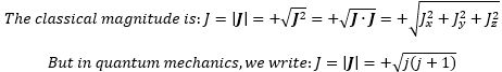 In this particular case (spin-1/2 particles), j is equal to 1/2 (in units of ħ, of course). Hence, J is equal to √0.75 ≈ 0.866. Elementary geometry then tells us cos(θ) = (1/2)/√(3/4) = = 1/√3. Hence, θ ≈ 54.73561°. That’s a big angle—larger than the 45° angle we had secretly expected because… Well… The 45° angle has that √2 factor in it: cos(45°) = sin(45°) = 1/√2.
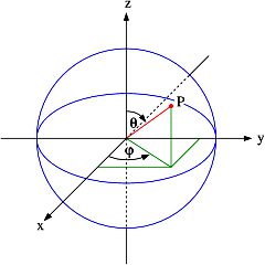 They are oscillations, still, so I am not thinking of two flywheels that keep going around in the same direction. No. More like a wobbling object on a spring. Something like the movement of a bobblehead on a spring perhaps. 🙂


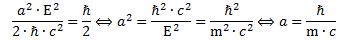
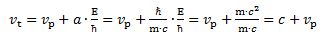
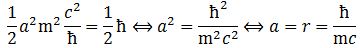
 We can write this as a function of m and the c and ħ constants only:
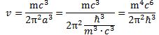


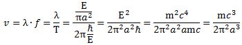
 We can re-write this as:
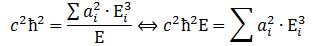 What is the meaning of this equation? We may look at it as some sort of physical normalization condition when building up the Fourier sum. Of course, we should relate this to the mathematical normalization condition for the wavefunction. Our intuition tells us that the probabilities must be related to the energy densities, but how exactly? We will come back to this question in a moment. Let us first think some more about the enigma: what is mass?
 This reminds us of the ω2= C–1/L or ω2 = k/m of harmonic oscillators once again.
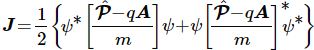
 Hence, if the electric field vector E is expressed in force per unit charge (N/C), then we may want to think of associating the real part of our wavefunction with a force per unit mass (N/kg). We can, of course, do a substitution here, because the mass unit (1 kg) is equivalent to 1 N·s2/m. Hence, our N/kg dimension becomes:
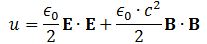 E and B are the electric and magnetic field vector respectively. The Poynting vector will give us the directional energy flux, i.e. the energy flow per unit area per unit time. We write:
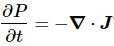
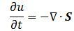 Needless to say, the ∇∙ operator is the divergence and, therefore, gives us the magnitude of a (vector) field’s source or sink at a given point. To be precise, the divergence gives us the volume density of the outward flux of a vector field from an infinitesimal volume around a given point. In this case, it gives us the volume density of the flux of S.
 Zero!? An unexpected result! Or not? We have no stationary charges and no currents: only an electromagnetic wave in free space. Hence, the local energy conservation principle needs to be respected at all points in space and in time. The geometry makes sense of the result: for an electromagnetic wave, the magnitudes of E and B reach their maximum, minimum and zero point simultaneously, as shown below.
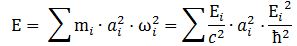
 We get what we hoped to get: the absolute square of our amplitude is, effectively, an energy density !


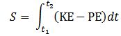 Now, we can choose any reference point for the potential energy but, to reflect the energy conservation law, we can select a reference point that ensures the sum of the kinetic and the potential energy is zero throughout the time interval. If the force field is uniform, then the integrand will, effectively, be equal to KE − PE = m·v2.
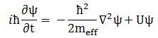 This formulation includes a term with the potential energy (U). In free space (no potential), this term disappears, and the equation can be re-written as:

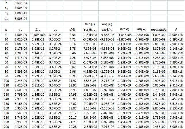
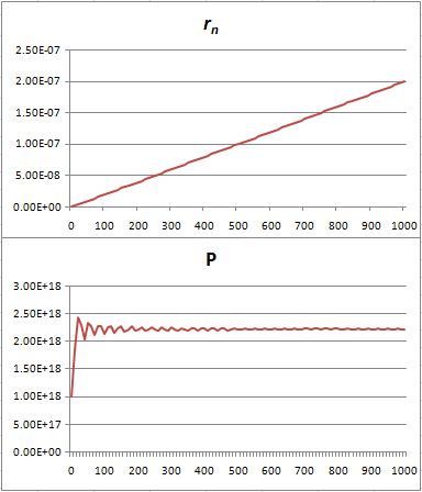
 Hence, if S0 is the action for r0, then S1 = S0 + ħ and S2 = S0 + 2·ħ are still good, but S3 = S0 + 3·ħ is not good. Why? Because the difference in the phase angles is Δθ = S1/ħ − S0/ħ = (S0 + ħ)/ħ − S0/ħ = 1 and Δθ = S2/ħ − S0/ħ = (S0 + 2·ħ)/ħ − S0/ħ = 2 respectively, so that’s 57.3° and 114.6° respectively and that’s, effectively, less than 120°. In contrast, for the next path, we find that Δθ = S3/ħ − S0/ħ = (S0 + 3·ħ)/ħ − S0/ħ = 3, so that’s 171.9°. So that amplitude gives us a negative contribution.
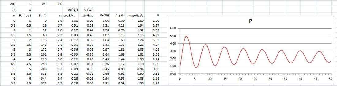 Well… We get a weird result. It reminds me of
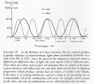

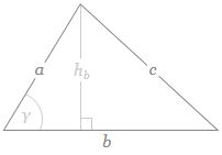 If b is the straight-line path (r0), then ac could be one of the crooked paths (rn). To simplify, we’ll assume isosceles triangles, so a equals c and, hence, rn = 2·a = 2·c. We will also assume the successive paths are separated by the same vertical distance (h = h1) right in the middle, so hb = hn = n·h1. It is then easy to show the following:
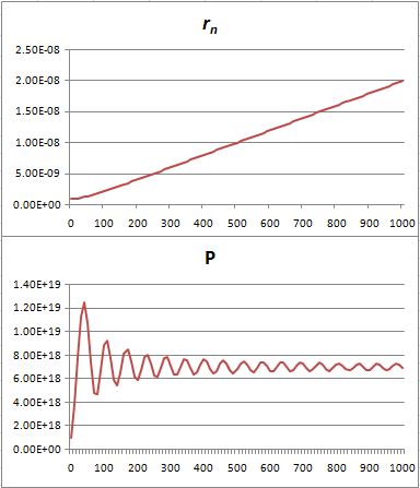

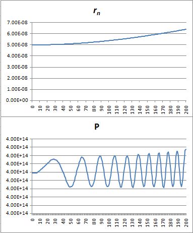 That’s because we increase the weight of the paths that are further removed from the center. So… Well… We shouldn’t be doing that, I guess. 🙂 I’ll you look for the right formula, OK? Let me know when you found it. 🙂
 We know this elementary wavefunction cannot represent a real-life particle. Indeed, the a·e−i·θ function implies the probability of finding the particle – an electron, a photon, or whatever – would be equal to P(x, t) = |ψ(x, t)|2 = |a·e−(i/ħ)·(E·t−p·x)|2 = |a|2·|e−(i/ħ)·(E·t−p·x)|2 = |a|2·12= a2 everywhere. Hence, the particle would be everywhere – and, therefore, nowhere really. We need to localize the wave – or build a wave packet. We can do so by introducing uncertainty: we then add a potentially infinite number of these elementary wavefunctions with slightly different values for E and p, and various amplitudes a. Each of these amplitudes will then reflect the contribution to the composite wave, which – in three-dimensional space – we can write as:
 Hence, if we don’t change the direction of the y– and z-axes – so we keep defining the z-axis as the axis pointing upwards, and the y-axis as the axis pointing towards us – then the positive direction of the x-axis would actually be the direction from right to left, and we should say that the elementary wavefunction in the animation above seems to propagate in the negative x-direction. [Note that this left- or right-hand rule is quite astonishing: simply swapping the direction of one axis of a left-handed frame makes it right-handed, and vice versa.]

 The next illustration – of how water waves actually propagate – is, perhaps, more relevant. Just think of a two-dimensional equivalent – and of the two oscillations as being transverse waves, as opposed to longitudinal. See how string theory starts making sense? 🙂
 The most fundamental question remains the same: what is it, exactly, that is oscillating here? What is the field? It’s always some force on some charge – but what charge, exactly? Mass? What is it? Well… I don’t have the answer to that. It’s the same as asking: what is electric charge, really? So the question is: what’s the reality of mass, of electric charge, or whatever other charge that causes a force to act on it?
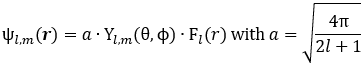 Note
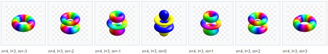
Note 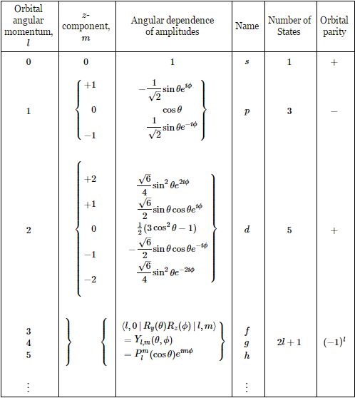 The Plm(cosθ) functions are the so-called
 So… To make a long story short, we can substitute the cosθ argument in the Plm(cosθ) function for sinα = sin(π/2 − θ). Now, if the xy-plane is a symmetry plane, then we must find the same value for Plm(sinα) and Plm[sin(−α)]. Now, that’s not obvious, because sin(−α) = −sinα ≠ sinα. However, because the argument in that Plm(x) function is being squared before any other operation (like subtracting 1 and exponentiating the result), it is OK: [−sinα]2 = [sinα]2 = sin2α. […] OK, I am sure the geeks amongst my readers will be able to explain this more rigorously. In fact, I hope they’ll have a look at it, because there’s also that dl+m/dxl+m operator, and so you should check what happens with the minus sign there. 🙂