Pre-scriptum (dated 26 June 2020): These posts on elementary math and physics for my kids (they are 21 and 23 now and no longer need such explanations) have not suffered much the attack by the dark force—which is good because I still like them. While my views on the true nature of light, matter and the force or forces that act on them have evolved significantly as part of my explorations of a more realist (classical) explanation of quantum mechanics, I think most (if not all) of the analysis in this post remains valid and fun to read. In fact, I find the simplest stuff is often the best. 🙂
Original post:
I wrote this post to just briefly entertain myself and my teenage kids. To be precise, I am writing this for Vincent, as he started to study more math this year (eight hours a week!), and as he also thinks he might go for engineering studies two years from now. So let’s see if he gets this and − much more importantly − if he likes the topic. If not… Well… Then he should get even better at golf than he already is, so he can make a living out of it. 🙂
To be sure, nothing what I write below requires an understanding of stuff you haven’t seen yet, like integrals, or complex numbers. There’s no derivatives, exponentials or logarithms either: you just need to know what a sine or a cosine is, and then it’s just a bit of addition and multiplication. So it’s just… Well… Geometry and waves as I would teach it to an interested teenager. So let’s go for it. And, yes, I am talking to you now, Vincent! 🙂
The animation below shows a repeating pulse. It is a periodic function: a traveling wave. It obviously travels in the positive x-direction, i.e. from left to right as per our convention. As you can see, the amplitude of our little wave varies as a function of time (t) and space (x), so it’s a function in two variables, like y = F(u, v). You know what that is, and you also know we’d refer to y as the dependent variable and to u and v as the independent variables.
Now, because it’s a wave, and because it travels in the positive x-direction, the argument of the wave function F will be x−ct, so we write:
y = F(x−ct)
Just to make sure: c is the speed of travel of this particular wave, so don’t think it’s the speed of light. This wave can be any wave: a water wave, a sound wave,… Whatever. Our dependent variable y is the amplitude of our wave, so it’s the vertical displacement − up or down − of whatever we’re looking at. As it’s a repeating pulse, y is zero most of the time, except when that pulse is pulsing. 🙂
So what’s the wavelength of this thing?
[…] Come on, Vincent. Think! Don’t just look at this!
[…] I got it, daddy! It’s the distance between two peaks, or between the center of two successive pulses— obviously! 🙂
[…] Good! 🙂 OK. That was easy enough. Now look at the argument of this function once again:
F = F(x−ct)
We are not merely acknowledging here that F is some function of x and t, i.e. some function varying in space and time. Of course, F is that too, so we can write: y = F = F(x, t) = F(x−ct), but it’s more than just some function: we’ve got a very special argument here, x−ct, and so let’s start our little lesson by explaining it.
The x−ct argument is there because we’re talking waves, so that is something moving through space and time indeed. Now, what are we actually doing when we write x−ct? Believe it or not, we’re basically converting something expressed in time units into something expressed in distance units. So we’re converting time into distance, so to speak. To see how this works, suppose we add some time Δt to the argument of our function y = F, so we’re looking at F[x−c(t+Δt)] now, instead of F(x−ct). Now, F[x−c(t+Δt)] = F(x−ct−cΔt), so we’ll get a different value for our function—obviously! But it’s easy to see that we can restore our wave function F to its former value by also adding some distance Δx = cΔt to the argument. Indeed, if we do so, we get F[x+Δx−c(t+Δt)] = F(x+cΔt–ct−cΔt) = F(x–ct). For example, if c = 3 m/s, then 2 seconds of time correspond to (2 s)×(3 m/s) = 6 meters of distance.
The idea behind adding both some time Δt as well as some distance Δx is that you’re traveling with the waveform itself, or with its phase as they say. So it’s like you’re riding on its crest or in its trough, or somewhere hanging on to it, so to speak. Hence, the speed of a wave is also referred to as its phase velocity, which we denote by vp = c. Now, let me make some remarks here.
First, there is the direction of travel. The pulses above travel in the positive x-direction, so that’s why we have x minus ct in the argument. For a wave traveling in the negative x-direction, we’ll have a wave function y = F(x+ct). [And, yes, don’t be lazy, Vincent: please go through the Δx = cΔt math once again to double-check that.]
The second thing you should note is that the speed of a regular periodic wave is equal to to the product of its wavelength and its frequency, so we write: vp = c = λ·f, which we can also write as λ = c/f or f = c/λ. Now, you know we express the frequency in oscillations or cycles per second, i.e. in hertz: one hertz is, quite simply, 1 s−1, so the unit of frequency is the reciprocal of the second. So the m/s and the Hz units in the fraction below give us a wavelength λ equal to λ = (20 m/s)/(5/s) = 4 m. You’ll say that’s too simple but I just want to make sure you’ve got the basics right here.
The third thing is that, in physics, and in math, we’ll usually work with nice sinusoidal functions, i.e. sine or cosine functions. A sine and a cosine function are the same function but with a phase difference of 90 degrees, so that’s π/2 radians. That’s illustrated below: cosθ = sin(θ+π/2).
Now, when we converted time to distance by multiplying it with c, what we actually did was to ensure that the argument of our wavefunction F was expressed in one unit only: the meter, so that’s the distance unit in the international SI system of units. So that’s why we had to convert time to distance, so to speak.
The other option is to express all in seconds, so that’s in time units. So then we should measure distance in seconds, rather than meters, so to speak, and the corresponding argument is t–x/c, and our wave function would be written as y = G(t–x/c). Just go through the same Δx = cΔt math once more: G[t+Δt–(x+Δx)/c] = G(t+Δt–x/c−cΔt/c) = G(t–x/c).
In short, we’re talking the same wave function here, so F(x−ct) = G(t−x/c), but the argument of F is expressed in distance units, while the argument of G is expressed in time units. If you’d want to double-check what I am saying here, you can use the same 20 m/s wave example again: suppose the distance traveled is 100 m, so x = 100 m and x/c = (100 m)/(20 m/s) = 5 seconds. It’s always important to check the units, and you can see they come out alright in both cases! 🙂
Now, to go from F or G to our sine or cosine function, we need to do yet another conversion of units, as the argument of a sinusoidal function is some angle θ, not meters or seconds. In physics, we refer to θ as the phase of the wave function. So we need degrees or, more common now, radians, which I’ll explain in a moment. Let me first jot it down:
y = sin(2π(x–ct)/λ)
So what are we doing here? What’s going on? Well… First, we divide x–ct by the wavelength λ, so that’s the (x–ct)/λ in the argument of our sine function. So our ‘distance unit’ is no longer the meter but the wavelength of our wave, so we no longer measure in meter but in wavelengths. For example, if our argument x–ct was 20 m, and the wavelength of our wave is 4 m, we get (x–ct)/λ = 5 between the brackets. It’s just like comparing our length: ten years ago you were about half my size. Now you’re the same: one unit. 🙂 When we’re saying that, we’re using my length as the unit – and so that’s also your length unit now 🙂 – rather than meters or centimeters.
Now I need to explain the 2π factor, which is only slightly more difficult. Think about it: one wavelength corresponds to one full cycle, so that’s the full 360° of the circle below. In fact, we’ll express angles in radians, and the two animations below illustrate what a radian really is: an angle of 1 rad defines an arc whose length, as measured on the circle, is equal to the radius of that circle. […] Oh! Please look at the animations as two separate things: they illustrate the same idea, but they’re not synchronized, unfortunately! 🙂
So… I hope it all makes sense now: if we add one wavelength to the argument of our wave function, we should get the same value, and so it’s equivalent to adding 2π to the argument of our sine function. Adding half a wavelength, or 35% of it, or a quarter, or two wavelengths, or e wavelengths, etc is equivalent to adding π, or 35%·2π ≈ 2.2, or 2π/4 = π/2, or 2·2π = 4π, or e·2π, etc to it. So… Well… Think about it: to go from the argument of our wavefunction expressed as a number of wavelengths − so that’s (x–ct)/λ – to the argument of our sine function, which is expressed in radians, we need to multiply by 2π.
[…] OK, Vincent. If it’s easier for you, you may want to think of the 1/λ and 2π factors in the argument of the sin(2π(x–ct)/λ) function as scaling factors: you’d use a scaling factor when you go from one measurement scale to another indeed. It’s like using vincents rather than meter. If one vincent corresponds to 1.8 m, then we need to re-scale all lengths by dividing them by 1.8 so as to express them in vincents. Vincent ten year ago was 0.9 m, so that’s half a vincent: 0.9/1.8 = 0.5. 🙂
[…] OK. […] Yes, you’re right: that’s rather stupid and makes nobody smile. Fine. You’re right: it’s time to move on to more complicated stuff. Now, read the following a couple of times. It’s my one and only message to you:
If there’s anything at all that you should remember from all of the nonsense I am writing about in this physics blog, it’s that any periodic phenomenon, any motion really, can be analyzed by assuming that it is the sum of the motions of all the different modes of what we’re looking at, combined with appropriate amplitudes and phases.
It really is a most amazing thing—it’s something very deep and very beautiful connecting all of physics with math.
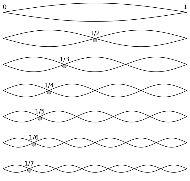
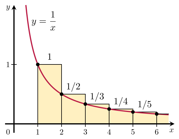
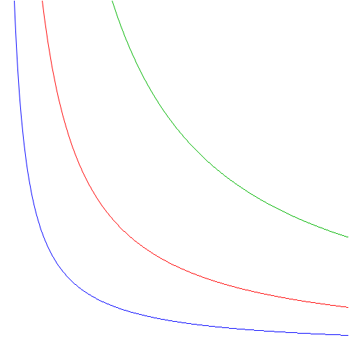
We often refer to these modes as harmonics and, in one of my posts on the topic, I explained how the wavelengths of the harmonics of a classical guitar string – it’s just an example – depended on the length of the string only. Indeed, if we denote the various harmonics by their harmonic number n = 1, 2, 3,… n,… and the length of the string by L, we have λ1 = 2L = (1/1)·2L, λ2 = L = (1/2)·2L, λ3 = (1/3)·2L,… λn = (1/n)·2L. So they look like this:

etcetera (1/8, 1/9,…,1/n,… 1/∞)
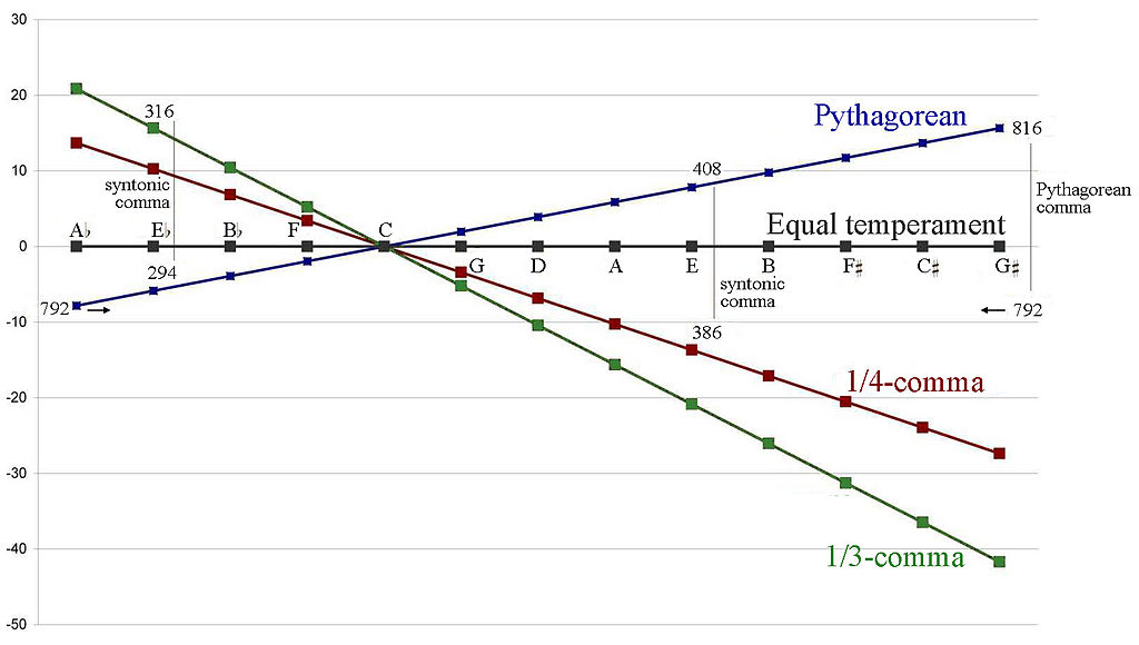
The diagram makes it look like it’s very obvious, but it’s an amazing fact: the material of the string, or its tension, doesn’t matter. It’s just the length: simple geometry is all that matters! As I mentioned in my post on music and physics, this realization led to a somewhat misplaced fascination with harmonic ratios, which the Greeks thought could explain everything. For example, the Pythagorean model of the orbits of the planets would also refer to these harmonic ratios, and it took intellectual giants like Galileo and Copernicus to finally convince the Pope that harmonic ratios are great, but that they cannot explain everything. 🙂 [Note: When I say that the material of the string, or its tension, doesn’t matter, I should correct myself: they do come into play when time becomes the variable. Also note that guitar strings are not the same length when strung on a guitar: the so-called bridge saddle is not in an exact right angle to the strings: this is a link to some close-up pictures of a bridge saddle on a guitar, just in case you don’t have a guitar at home to check.]
Now, I already explained the need to express the argument of a wave function in radians – because we’re talking periodic functions and so we want to use sinusoidals − and how it’s just a matter of units really, and so how we can go from meter to wavelengths to radians. I also explained how we could do the same for seconds, i.e. for time. The key to converting distance units to time units, and vice versa, is the speed of the wave, or the phase velocity, which relates wavelength and frequency: c = λ·f. Now, as we have to express everything in radians anyway, we’ll usually substitute the wavelength and frequency by the wavenumber and the angular frequency so as to convert these quantities too to something expressed in radians. Let me quickly explain how it works:
- The wavenumber k is equal to k = 2π/λ, so it’s some number expressed in radians per unit distance, i.e. radians per meter. In the example above, where λ was 4 m, we have k = 2π/(4 m) = π/2 radians per meter. To put it differently, if our wave travels one meter, its phase θ will change by π/2.
- Likewise, the angular frequency is ω = 2π·f = 2π/T. Using the same example once more, so assuming a frequency of 5 Hz, i.e. a period of one fifth of a second, we have ω = 2π/[(1/5)·s] = 10π per second. So the phase of our wave will change with 10 times π in one second. Now that makes sense because, in one second, we have five cycles, and so that corresponds to 5 times 2π.
Note that our definition implies that λ = 2π/k, and that it’s also easy to figure out that our definition of ω, combined with the f = c/λ relation, implies that ω = 2π·c/λ and, hence, that c = ω·λ/(2π) = (ω·2π/k)/(2π) = ω/k. OK. Let’s move on.
Using the definitions and explanations above, it’s now easy to see that we can re-write our y = sin(2π(x–ct)/λ) as:
y = sin(2π(x–ct)/λ) = sin[2π(x–(ω/k)t)/(2π/k)] = sin[(x–(ω/k)t)·k)] = sin(kx–ωt)
Remember, however, that we were talking some wave that was traveling in the positive x-direction. For the negative x-direction, the equation becomes:
y = sin(2π(x+ct)/λ) = sin(kx+ωt)
OK. That should be clear enough. Let’s go back to our guitar string. We can go from λ to k by noting that λ = 2L and, hence, we get the following for all of the various modes:
k = k1 = 2π·1/(2L) = π/L, k2 = 2π·2/(2L) = 2k, k3 = 2π·3/(2L) = 3k,,… kn = 2π·3/(2L) = nk,…
That gives us our grand result, and that’s that we can write some very complicated waveform Ψ(x) as the sum of an infinite number of simple sinusoids, so we have:
Ψ(x) = a1sin(kx) + a2sin(2kx) + a3sin(3kx) + … + ansin(nkx) + … = ∑ ansin(nkx)
The equation above assumes we’re looking at the oscillation at some fixed point in time. If we’d be looking at the oscillation at some fixed point in space, we’d write:
Φ(t) = a1sin(ωt) + a2sin(2ωt) + a3sin(3ωt) + … + ansin(nωt) + … = ∑ ansin(nωt)
Of course, to represent some very complicated oscillation on our guitar string, we can and should combine some Ψ(x) as well as some Φ(t) function, but how do we do that, exactly? Well… We’ll obviously need both the sin(kx–ωt) as well as those sin(kx+ωt) functions, as I’ll explain in a moment. However, let me first make another small digression, so as to complete your knowledge of wave mechanics. 🙂
We look at a wave as something that’s traveling through space and time at the same time. In that regard, I told you that the speed of the wave is its so-called phase velocity, which we denoted as vp = c and which, as I explained above, is equal to vp = c = λ·f = (2π/k)·(ω/2π) = ω/k. The animation below (credit for it must go to Wikipedia—and sorry I forget to acknowledge the same source for the illustrations above) illustrates the principle: the speed of travel of the red dot is the phase velocity. But you can see that what’s going on here is somewhat more complicated: we have a series of wave packets traveling through space and time here, and so that’s where the concept of the so-called group velocity comes in: it’s the speed of travel of the green dot.

Now, look at the animation below. What’s going on here? The wave packet (or the group or the envelope of the wave—whatever you want to call it) moves to the right, but the phase goes to the left, as the peaks and troughs move leftward indeed. Huh? How is that possible? And where is this wave going? Left or right? Can we still associate some direction with the wave here? It looks like it’s traveling in both directions at the same time!
The wave actually does travel in both directions at the same time. Well… Sort of. The point is actually quite subtle. When I started this post by writing that the pulses were ‘obviously’ traveling in the positive x-direction… Well… That’s actually not so obvious. What is it that is traveling really? Think about an oscillating guitar string: nothing travels left or right really. Each point on the string just moves up and down. Likewise, if our repeated pulse is some water wave, then the water just stays where it is: it just moves up and down. Likewise, if we shake up some rope, the rope is not going anywhere: we just started some motion that is traveling down the rope. In other words, the phase velocity is just a mathematical concept. The peaks and troughs that seem to be traveling are just mathematical points that are ‘traveling’ left or right.
What about the group velocity? Is that a mathematical notion too? It is. The wave packet is often referred to as the envelope of the wave curves, for obviously reasons: they’re enveloped indeed. Well… Sort of. 🙂 However, while both the phase and group velocity are velocities of mathematical constructs, it’s obvious that, if we’re looking at wave packets, the group velocity would be of more interest to us than the phase velocity. Think of those repeated pulses as real water waves, for example: while the water stays where it is (as mentioned, the water molecules just go up and down—more or less, at least), we’d surely be interested to know how fast these waves are ‘moving’, and that’s given by the group velocity, not the phase velocity. Still, having said that, the group velocity is as ‘unreal’ as the phase velocity: both are mathematical concepts. The only thing that’s ‘real’ is the up and down movement. Nothing travels in reality. Now, I shouldn’t digress too much here, but that’s why there’s no limit on the phase velocity: it can exceed the speed of light. In fact, in quantum mechanics, some real-life particle − like an electron, for instance – will be represented by a complex-valued wave function, and there’s no reason to put some limit on the phase velocity. In contrast, the group velocity will actually be the speed of the electron itself, and that speed can, obviously, approach the speed of light – in particle accelerators, for example – but it can never exceed it. [If you’re smart, and you are, you’ll wonder: what about photons? Well…The classical and quantum-mechanical view of an electromagnetic wave are surely not the same, but they do have a lot in common: both photons and electromagnetic radiation travel at the speed c. Photons can do so because their rest mass is zero. But I can’t go into any more detail here, otherwise this thing will become way too long.]
OK. Let me get back to the issue at hand. So I’ll now revert to the simpler situation we’re looking at here, and so that’s these harmonic waves, whose form is a simple sinusoidal indeed. The animation below (and, yes, it’s also from Wikipedia) is the one that’s relevant for this situation. You need to study it for a while to understand what’s going on. As you can see, the green wave travels to the right, the blue one travels to the left, and the red wave function is the sum of both.
Of course, after all that I wrote above, I should use quotation marks and write ‘travel’ instead of travel, so as to indicate there’s nothing traveling really, except for those mathematical points, but then no one does that, and so I won’t do it either. Just make sure you always think twice when reading stuff like this! Back to the lesson: what’s going on here?
As I explained, the argument of a wave traveling towards the negative x-direction will be x+ct. Conversely, the argument of a wave traveling in the positive x-direction will be x–ct. Now, our guitar string is going nowhere, obviously: it’s like the red wave function above. It’s a so-called standing wave. The red wave function has nodes, i.e. points where there is no motion—no displacement at all! Between the nodes, every point moves up and down sinusoidally, but the pattern of motion stays fixed in space. So that’s the kind of wave function we want, and the animation shows us how we can get it.
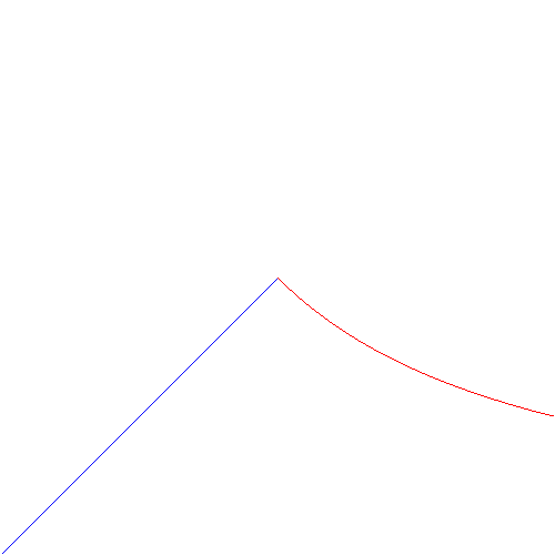
Indeed, there’s a funny thing with fixed strings: when a wave reaches the clamped end of a string, it will be reflected with a change in sign, as illustrated below: we’ve got that F(x+ct) wave coming in, and then it goes back indeed, but with the sign reversed.

The illustration above speaks for itself but, of course, once again I need to warn you about the use of sentences like ‘the wave reaches the end of the string’ and/or ‘the wave gets reflected back’. You know what it really means now: it’s some movement that travels through space. […] In any case, let’s get back to the lesson once more: how do we analyze that?
Easy: the red wave function is the sum of two waves: one traveling to the right, and one traveling to the left. We’ll call these component waves F and G respectively, so we have y = F(x, t) + G(x, t). Let’s go for it.
Let’s first assume the string is not held anywhere, so that we have an infinite string along which waves can travel in either direction. In fact, the most general functional form to capture the fact that a waveform can travel in any direction is to write the displacement y as the sum of two functions: one wave traveling one way (which we’ll denote by F, indeed), and the other wave (which, yes, we’ll denote by G) traveling the other way. From the illustration above, it’s obvious that the F wave is traveling towards the negative x-direction and, hence, its argument will be x+ct. Conversely, the G wave travels in the positive x-direction, so its argument is x–ct. So we write:
y = F(x, t) + G(x, t) = F(x+ct) + G(x–ct)
So… Well… We know that the string is actually not infinite, but that it’s fixed to two points. Hence, y is equal to zero there: y = 0. Now let’s choose the origin of our x-axis at the fixed end so as to simplify the analysis. Hence, where y is zero, x is also zero. Now, at x = 0, our general solution above for the infinite string becomes y = F(ct) + G(−ct) = 0, for all values of t. Of course, that means G(−ct) must be equal to –F(ct). Now, that equality is there for all values of t. So it’s there for all values of ct and −ct. In short, that equality is valid for whatever value of the argument of G and –F. As Feynman puts it: “G of anything must be –F of minus that same thing.” Now, the ‘anything’ in G is its argument: x – ct, so ‘minus that same thing’ is –(x–ct) = −x+ct. Therefore, our equation becomes:
y = F(x+ct) − F(−x+ct)
So that’s what’s depicted in the diagram above: the F(x+ct) wave ‘vanishes’ behind the wall as the − F(−x+ct) wave comes out of it. Now, of course, so as to make sure our guitar string doesn’t stop its vibration after being plucked, we need to ensure F is a periodic function, like a sin(kx+ωt) function. 🙂 Why? Well… If this F and G function would simply disappear and ‘serve’ only once, so to speak, then we only have one oscillation and that’s it! So the waves need to continue and so that’s why it needs to be periodic.
OK. Can we just take sin(kx+ωt) and −sin(−kx+ωt) and add both? It makes sense, doesn’t it? Indeed, −sinα = sin(−α) and, therefore, −sin(−kx+ωt) = sin(kx−ωt). Hence, y = F(x+ct) − F(−x+ct) would be equal to:
y = sin(kx+ωt) + sin(kx–ωt) = sin(2π(x+ct)/λ) + sin(2π(x−ct)/λ)
Done! Let’s use specific values for k and ω now. For the first harmonic, we know that k = 2π/2L = π/L. What about ω? Hmm… That depends on the wave velocity and, therefore, that actually does depend on the material and/or the tension of the string! The only thing we can say is that ω = c·k, so ω = c·2π/λ = c·π/L. So we get:
sin(kx+ωt) = sin(π·x/L + π·c·t/L) = sin[(π/L)·(x+ct)]
But this is our F function only. The whole oscillation is y = F(x+ct) − F(−x+ct), and − F(−x+ct) is equal to:
–sin[(π/L)·(−x+ct)] = –sin(−π·x/L+π·c·t/L) = −sin(−kx+ωt) = sin(kx–ωt) = sin[(π/L)·(x–ct)]
So, yes, we should add both functions to get:
y = sin[π(x+ct)/L] + sin[π(x−ct)/L]
Now, we can, of course, apply our trigonometric formulas for the addition of angles, which say that sin(α+β) = sinαcosβ + sinβcosα and sin(α–β) = sinαcosβ – sinβcosα. Hence, y = sin(kx+ωt) + sin(kx–ωt) is equal to sin(kx)cos(ωt) + sin(ωt)cos(kx) + sin(kx)cos(ωt) – sin(ωt)cos(kx) = 2sin(kx)cos(ωt). Now, that’s a very interesting result, so let’s give it some more prominence by writing it in boldface:
y = sin(kx+ωt) + sin(kx–ωt) = 2sin(kx)cos(ωt) = 2sin(π·x/L)cos(π·c·t/L)
The sin(π·x/L) factor gives us the nodes in space. Indeed, sin(π·x/L) = 0 if x is equal to 0 or L (values of x outside of the [0, L] interval are obviously not relevant here). Now, the other factor cos(π·c·t/L) can be re-written cos(2π·c·t/λ) = cos(2π·f·t) = cos(2π·t/T), with T the period T = 1/f = λ/c, so the amplitude reaches a maximum (+1 or −1 or, including the factor 2, +2 or −2) if 2π·t/T is equal to a multiple of π, so that’s if t = n·T/2 with n = 0, 1, 2, etc. In our example above, for f = 5 Hz, that means the amplitude reaches a maximum (+2 or −2) every tenth of a second.
The analysis for the other modes is as easy, and I’ll leave it you, Vincent, as an exercise, to work it all out and send me the y = 2·sin[something]·cos[something else] formula (with the ‘something’ and ‘something else’ written in terms of L and c, of course) for the higher harmonics. 🙂
[…] You’ll say: what’s the point, daddy? Well… Look at that animation again: isn’t it great we can analyze any standing wave, or any harmonic indeed, as the sum of two component waves with the same wavelength and frequency but ‘traveling’ in opposite directions?
Yes, Vincent. I can hear you sigh: “Daddy, I really do not see why I should be interested in this.”
Well… Your call… What can I say? Maybe one day you will. In fact, if you’re going to go for engineering studies, you’ll have to. 🙂
To conclude this post, I’ll insert one more illustration. Now that you know what modes are, you can start thinking about those more complicated Ψ and Φ functions. The illustration below shows how the first and second mode of our guitar string combine to give us some composite wave traveling up and down the very same string.

Think about it. We have one physical phenomenon here: at every point in time, the string is somewhere, but where exactly, depends on the mathematical shape of its components. If this doesn’t illustrate the beauty of Nature, the fact that, behind every simple physical phenomenon − most of which are some sort of oscillation indeed − we have some marvelous mathematical structure, then… Well… Then I don’t know how to explain why I am absolutely fascinated by this stuff.
Addendum 1: On actual waves
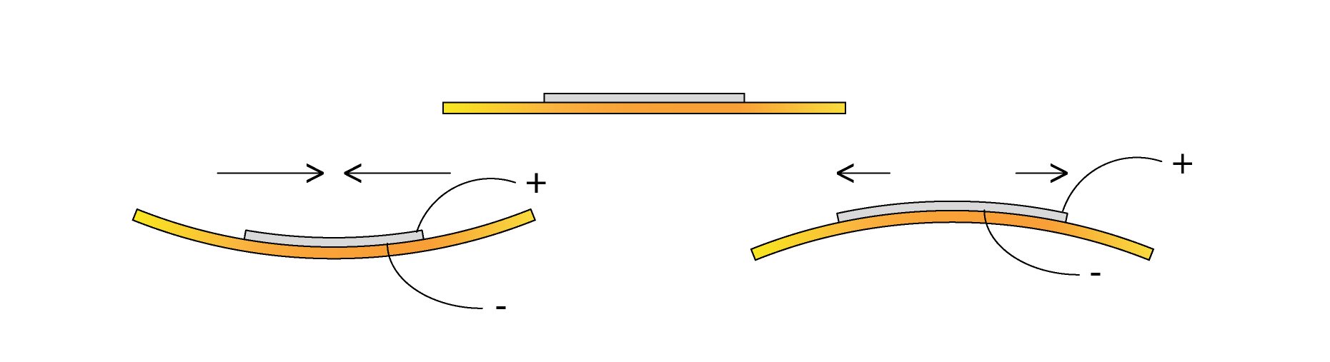
My examples of waves above were all examples of so-called transverse waves, i.e. oscillations at a right angle to the direction of the wave. The other type of wave is longitudinal. I mentioned sound waves above, but they are essentially longitudinal. So there the displacement of the medium is in the same direction of the wave, as illustrated below.
Real-life waves, like water waves, may be neither of the two. The illustration below shows how water molecules actually move as a wave passes. They move in little circles, with a systemic phase shift from circle to circle.

Why is this so? I’ll let Feynman answer, as he also provided the illustration above:
“Although the water at a given place is alternately trough or hill, it cannot simply be moving up and down, by the conservation of water. That is, if it goes down, where is the water going to go? The water is essentially incompressible. The speed of compression of waves—that is, sound in the water—is much, much higher, and we are not considering that now. Since water is incompressible on this scale, as a hill comes down the water must move away from the region. What actually happens is that particles of water near the surface move approximately in circles. When smooth swells are coming, a person floating in a tire can look at a nearby object and see it going in a circle. So it is a mixture of longitudinal and transverse, to add to the confusion. At greater depths in the water the motions are smaller circles until, reasonably far down, there is nothing left of the motion.”
So… There you go… 🙂
Addendum 2: On non-periodic waves, i.e. pulses
A waveform is not necessarily periodic. The pulse we looked at could, perhaps, not repeat itself. It is not possible, then, to describe its wavelength. However, it’s still a wave and, hence, its functional form would still be some y = F(x−ct) or y = F(x+ct) form, depending on its direction of travel.
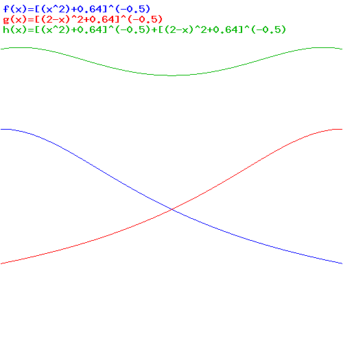
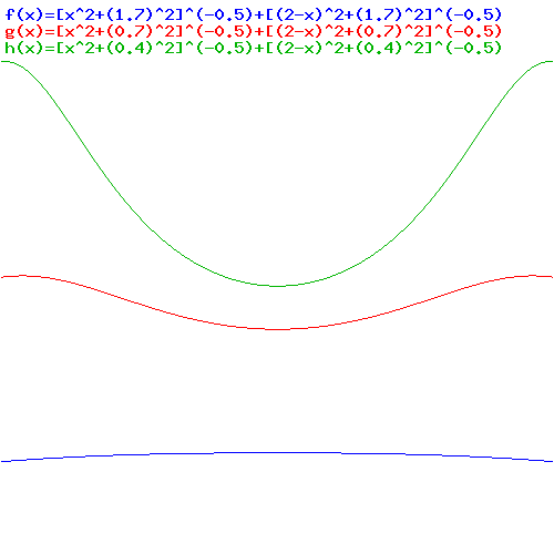
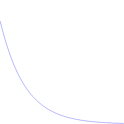
The example below also comes out of Feynman’s Lectures: electromagnetic radiation is caused by some accelerating electric charge – an electron, usually, because its mass is small and, hence, it’s much easier to move than a proton 🙂 – and then the electric field travels out in space. So the two diagrams below show (i) the acceleration (a) as a function of time (t) and (ii) the electric field strength (E) as a function of the distance (r). [To be fully precise, I should add he ignores the 1/r variation, but that’s a fine point which doesn’t matter much here.]
He basically uses this illustration to explain why we can use a y = G(t–x/c) functional form to describe a wave. The point is: he actually talks about one pulse only here. So the F(x±ct) or G(t±x/c) or sin(kx±ωt) form has nothing to do with whether or not we’re looking at a periodic or non-periodic waveform. The gist of the matter is that we’ve got something moving through space, and it doesn’t matter whether it’s periodic or not: the periodicity or non-periodicity, of a wave has nothing to do with the x±ct, t±x/c or kx±ωt shape of the argument of our wave function. The functional form of our argument is just the result of what I said about traveling along with our wave.
So what is it about periodicity then? Well… If periodicity kicks it, you’ll talk sinusoidal functions, and so the circle will be needed once more. 🙂
Now, I mentioned we cannot associate any particular wavelength with such non-periodic wave. Having said that, it’s still possible to analyze this pulse as a sum of sinusoids through a mathematical procedure which is referred to as the Fourier transform. If you’re going for engineer, you’ll need to learn how to master this technique. As for now, however, you can just have a look at the Wikipedia article on it. 🙂
Some content on this page was disabled on June 16, 2020 as a result of a DMCA takedown notice from The California Institute of Technology. You can learn more about the DMCA here:
https://wordpress.com/support/copyright-and-the-dmca/
Some content on this page was disabled on June 16, 2020 as a result of a DMCA takedown notice from The California Institute of Technology. You can learn more about the DMCA here:
https://wordpress.com/support/copyright-and-the-dmca/


 Simply substituting symbols then gives us the solution for Ax:
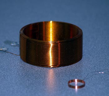
 with n the number of turns per unit length of the solenoid, and I the current going through it. However, in the mentioned post, we assumed that the magnetic field outside of the solenoid was zero, for all practical purposes, but it is not. It is very weak but not zero, as shown below. In fact, it’s fairly strong at very short distances from the solenoid! Calculating the vector potential allows us to calculate its exact value, everywhere. So let’s go for it.
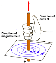
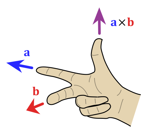 Also note the magnitude this formula implies: a×b = |a|·|b|·sinθ·n, with θ the angle between a and b, and n the normal unit vector in the direction given by that right-hand rule above. Now, unlike a vector dot product, the magnitude of the vector cross product is not zero for perpendicular vectors. In fact, when θ = π/2, which is the case for B0 and r’, then sinθ = 1, and, hence, we can write:


