Re-visiting uncertainty…

I re-visited the Uncertainty Principle a couple of times already, but here I really want to get at the bottom of the thing? What’s uncertain? The energy? The time? The wavefunction itself? These questions are not easily answered, and I need to warn you: you won’t get too much wiser when you’re finished reading this. I just felt like freewheeling a bit. [Note that the first part of this post repeats what you’ll find on the Occam page, or my post on Occam’s Razor. But these post do not analyze uncertainty, which is what I will be trying to do here.]

Let’s first think about the wavefunction itself. It’s tempting to think it actually is the particle, somehow. But it isn’t. So what is it then? Well… Nobody knows. In my previous post, I said I like to think it travels with the particle, but then doesn’t make much sense either. It’s like a fundamental property of the particle. Like the color of an apple. But where is that color? In the apple, in the light it reflects, in the retina of our eye, or is it in our brain? If you know a thing or two about how perception actually works, you’ll tend to agree the quality of color is not in the apple. When everything is said and done, the wavefunction is a mental construct: when learning physics, we start to think of a particle as a wavefunction, but they are two separate things: the particle is reality, the wavefunction is imaginary.

But that’s not what I want to talk about here. It’s about that uncertainty. Where is the uncertainty? You’ll say: you just said it was in our brain. No. I didn’t say that. It’s not that simple. Let’s look at the basic assumptions of quantum physics:

Quantum physics assumes there’s always some randomness in Nature and, hence, we can measure probabilities only. We’ve got randomness in classical mechanics too, but this is different. This is an assumption about how Nature works: we don’t really know what’s happening. We don’t know the internal wheels and gears, so to speak, or the ‘hidden variables’, as one interpretation of quantum mechanics would say. In fact, the most commonly accepted interpretation of quantum mechanics says there are no ‘hidden variables’.
However, as Shakespeare has one of his characters say: there is a method in the madness, and the pioneers– I mean Werner Heisenberg, Louis de Broglie, Niels Bohr, Paul Dirac, etcetera – discovered that method: all probabilities can be found by taking the square of the absolute value of a complex-valued wavefunction (often denoted by Ψ), whose argument, or phase (θ), is given by the de Broglie relations ω = E/ħ and k = p/ħ. The generic functional form of that wavefunction is:

Ψ = Ψ(x, t) = a·e^−iθ= a·e^{−i(ω·t − k ∙x)} = a·e^{−i·[(E/ħ)·t − (p/ħ)∙x]}

That should be obvious by now, as I’ve written more than a dozens of posts on this. 🙂 I still have trouble interpreting this, however—and I am not ashamed, because the Great Ones I just mentioned have trouble with that too. It’s not that complex exponential. That e^−iφ is a very simple periodic function, consisting of two sine waves rather than just one, as illustrated below. [It’s a sine and a cosine, but they’re the same function: there’s just a phase difference of 90 degrees.]

No. To understand the wavefunction, we need to understand those de Broglie relations, ω = E/ħ and k = p/ħ, and then, as mentioned, we need to understand the Uncertainty Principle. We need to understand where it comes from. Let’s try to go as far as we can by making a few remarks:

Adding or subtracting two terms in math, (E/ħ)·t − (p/ħ)∙x, implies the two terms should have the same dimension: we can only add apples to apples, and oranges to oranges. We shouldn’t mix them. Now, the (E/ħ)·t and (p/ħ)·x terms are actually dimensionless: they are pure numbers. So that’s even better. Just check it: energy is expressed in newton·meter (energy, or work, is force over distance, remember?) or electronvolts (1 eV = 1.6×10⁻¹⁹J = 1.6×10⁻¹⁹N·m); Planck’s constant, as the quantum of action, is expressed in J·s or eV·s; and the unit of (linear) momentum is 1 N·s = 1 kg·m/s = 1 N·s. E/ħ gives a number expressed per second, and p/ħ a number expressed per meter. Therefore, multiplying E/ħ and p/ħ by t and x respectively gives us a dimensionless number indeed.
It’s also an invariant number, which means we’ll always get the same value for it, regardless of our frame of reference. As mentioned above, that’s because the four-vector product p_μx_μ= E·t − p∙x is invariant: it doesn’t change when analyzing a phenomenon in one reference frame (e.g. our inertial reference frame) or another (i.e. in a moving frame).
Now, Planck’s quantum of action h, or ħ – h and ħ only differ in their dimension: h is measured in cycles per second, while ħ is measured in radians per second: both assume we can at least measure one cycle – is the quantum of energy really. Indeed, if “energy is the currency of the Universe”, and it’s real and/or virtual photons who are exchanging it, then it’s good to know the currency unit is h, i.e. the energy that’s associated with one cycle of a photon. [In case you want to see the logic of this, see my post on the physical constants c, h and α.]
It’s not only time and space that are related, as evidenced by the fact that t − x itself is an invariant four-vector, E and p are related too, of course! They are related through the classical velocity of the particle that we’re looking at: E/p = c²/v and, therefore, we can write: E·β = p·c, with β = v/c, i.e. the relative velocity of our particle, as measured as a ratio of the speed of light. Now, I should add that the t − x four-vector is invariant only if we measure time and space in equivalent units. Otherwise, we have to write c·t − x. If we do that, so our unit of distance becomes c meter, rather than one meter, or our unit of time becomes the time that is needed for light to travel one meter, then c = 1, and the E·β = p·c becomes E·β = p, which we also write as β = p/E: the ratio of the energy and the momentum of our particle is its (relative) velocity.

Combining all of the above, we may want to assume that we are measuring energy and momentum in terms of the Planck constant, i.e. the ‘natural’ unit for both. In addition, we may also want to assume that we’re measuring time and distance in equivalent units. Then the equation for the phase of our wavefunctions reduces to:

θ = (ω·t − k ∙x) = E·t − p·x

Now, θ is the argument of a wavefunction, and we can always re-scale such argument by multiplying or dividing it by some constant. It’s just like writing the argument of a wavefunction as v·t–x or (v·t–x)/v = t –x/v with v the velocity of the waveform that we happen to be looking at. [In case you have trouble following this argument, please check the post I did for my kids on waves and wavefunctions.] Now, the energy conservation principle tells us the energy of a free particle won’t change. [Just to remind you, a ‘free particle’ means it’s in a ‘field-free’ space, so our particle is in a region of uniform potential.] So we can, in this case, treat E as a constant, and divide E·t − p·x by E, so we get a re-scaled phase for our wavefunction, which I’ll write as:

φ = (E·t − p·x)/E = t − (p/E)·x = t − β·x

Alternatively, we could also look at p as some constant, as there is no variation in potential energy that will cause a change in momentum, and the related kinetic energy. We’d then divide by p and we’d get (E·t − p·x)/p = (E/p)·t − x) = t/β − x, which amounts to the same, as we can always re-scale by multiplying it with β, which would again yield the same t − β·x argument.

The point is, if we measure energy and momentum in terms of the Planck unit (I mean: in terms of the Planck constant, i.e. the quantum of energy), and if we measure time and distance in ‘natural’ units too, i.e. we take the speed of light to be unity, then our Platonic wavefunction becomes as simple as:

Φ(φ) = a·e^−iφ= a·e^{−i(t − β·x)}

This is a wonderful formula, but let me first answer your most likely question: why would we use a relative velocity?Well… Just think of it: when everything is said and done, the whole theory of relativity and, hence, the whole of physics, is based on one fundamental and experimentally verified fact: the speed of light is absolute. In whatever reference frame, we will always measure it as 299,792,458 m/s. That’s obvious, you’ll say, but it’s actually the weirdest thing ever if you start thinking about it, and it explains why those Lorentz transformations look so damn complicated. In any case, this fact legitimately establishes c as some kind of absolute measure against which all speeds can be measured. Therefore, it is only natural indeed to express a velocity as some number between 0 and 1. Now that amounts to expressing it as the β = v/c ratio.

Let’s now go back to that Φ(φ) = a·e^−iφ= a·e^{−i(t − β·x)}wavefunction. Its temporal frequency ω is equal to one, and its spatial frequency k is equal to β = v/c. It couldn’t be simpler but, of course, we’ve got this remarkably simple result because we re-scaled the argument of our wavefunction using the energy and momentum itself as the scale factor. So, yes, we can re-write the wavefunction of our particle in a particular elegant and simple form using the only information that we have when looking at quantum-mechanical stuff: energy and momentum, because that’s what everything reduces to at that level.

So… Well… We’ve pretty much explained what quantum physics is all about here. You just need to get used to that complex exponential: e^−iφ = cos(−φ) + i·sin(−φ) = cos(φ) −i·sin(φ). It would have been nice if Nature would have given us a simple sine or cosine function. [Remember the sine and cosine function are actually the same, except for a phase difference of 90 degrees: sin(φ) = cos(π/2−φ) = cos(φ+π/2). So we can go always from one to the other by shifting the origin of our axis.] But… Well… As we’ve shown so many times already, a real-valued wavefunction doesn’t explain the interference we observe, be it interference of electrons or whatever other particles or, for that matter, the interference of electromagnetic waves itself, which, as you know, we also need to look at as a stream of photons , i.e. light quanta, rather than as some kind of infinitely flexible aether that’s undulating, like water or air.

However, the analysis above does not include uncertainty. That’s as fundamental to quantum physics as de Broglie‘s equations, so let’s think about that now.

Introducing uncertainty

Our information on the energy and the momentum of our particle will be incomplete: we’ll write E = E₀± σ_E, and p = p₀± σ_p. Huh? No ΔE or ΔE? Well… It’s the same, really, but I am a bit tired of using the Δ symbol, so I am using the σ symbol here, which denotes a standard deviation of some density function. It underlines the probabilistic, or statistical, nature of our approach.

The simplest model is that of a two-state system, because it involves two energy levels only: E = E₀± A, with A some constant. Large or small, it doesn’t matter. All is relative anyway. 🙂 We explained the basics of the two-state system using the example of an ammonia molecule, i.e. an NH₃molecule, so it consists on one nitrogen and three hydrogen atoms. We had two base states in this system: ‘up’ or ‘down’, which we denoted as base state | 1 〉 and base state | 2 〉 respectively. This ‘up’ and ‘down’ had nothing to do with the classical or quantum-mechanical notion of spin, which is related to the magnetic moment. No. It’s much simpler than that: the nitrogen atom could be either beneath or, else, above the plane of the hydrogens, as shown below, with ‘beneath’ and ‘above’ being defined in regard to the molecule’s direction of rotation around its axis of symmetry.

In any case, for the details, I’ll refer you to the post(s) on it. Here I just want to mention the result. We wrote the amplitude to find the molecule in either one of these two states as:

C₁= 〈 1 | ψ 〉 = (1/2)·e^{−(i/ħ)·(E₀− A)·t}+ (1/2)·e^{−(i/ħ)·(E₀+ A)·t}
C₂= 〈 2 | ψ 〉 = (1/2)·e^{−(i/ħ)·(E₀− A)·t}– (1/2)·e^{−(i/ħ)·(E₀+ A)·t}

That gave us the following probabilities:

If our molecule can be in two states only, and it starts off in one, then the probability that it will remain in that state will gradually decline, while the probability that it flips into the other state will gradually increase.

Now, the point you should note is that we get these time-dependent probabilities only because we’re introducing two different energy levels: E₀+ A and E₀− A. [Note they separated by an amount equal to 2·A, as I’ll use that information later.] If we’d have one energy level only – which amounts to saying that we know it, and that it’s something definite – then we’d just have one wavefunction, which we’d write as:

a·e^−iθ= a·e⁻⁽^{i/ħ)·(E₀·t − p·x)}= a·e⁻⁽ⁱ^/ħ)·(E^₀·t)·e⁽^{i/ħ)·(p·x)}

Note that we can always split our wavefunction in a ‘time’ and a ‘space’ part, which is quite convenient. In fact, because our ammonia molecule stays where it is, it has no momentum: p = 0. Therefore, its wavefunction reduces to:

a·e^−iθ= a·e⁻⁽^{i/ħ)·(E₀·t)}

As simple as it can be. 🙂 The point is that a wavefunction like this, i.e. a wavefunction that’s defined by a definite energy, will always yield a constant and equal probability, both in time as well as in space. That’s just the math of it: |a·e^−iθ|²= a². Always! If you want to know why, you should think of Euler’s formula and Pythagoras’ Theorem: cos²θ +sin²θ = 1. Always! 🙂

That constant probability is annoying, because our nitrogen atom never ‘flips’, and we know it actually does, thereby overcoming a energy barrier: it’s a phenomenon that’s referred to as ‘tunneling’, and it’s real! The probabilities in that graph above are real! Also, if our wavefunction would represent some moving particle, it would imply that the probability to find it somewhere in space is the same all over space, which implies our particle is everywhere and nowhere at the same time, really.

So, in quantum physics, this problem is solved by introducing uncertainty. Introducing some uncertainty about the energy, or about the momentum, is mathematically equivalent to saying that we’re actually looking at a composite wave, i.e. the sum of a finite or potentially infinite set of component waves. So we have the same ω = E/ħ and k = p/ħ relations, but we apply them to n energy levels, or to some continuous range of energy levels ΔE. It amounts to saying that our wave function doesn’t have a specific frequency: it now has n frequencies, or a range of frequencies Δω = ΔE/ħ. In our two-state system, n = 2, obviously! So we’ve two energy levels only and so our composite wave consists of two component waves only.

We know what that does: it ensures our wavefunction is being ‘contained’ in some ‘envelope’. It becomes a wavetrain, or a kind of beat note, as illustrated below:

[The animation comes from Wikipedia, and shows the difference between the group and phase velocity: the green dot shows the group velocity, while the red dot travels at the phase velocity.]

So… OK. That should be clear enough. Let’s now apply these thoughts to our ‘reduced’ wavefunction

Φ(φ) = a·e^−iφ= a·e^{−i(t − β·x)}

Thinking about uncertainty

Frankly, I tried to fool you above. If the functional form of the wavefunction is a·e⁻⁽^{i/ħ)·(E·t − p·x)}, then we can measure E and p in whatever unit we want, including h or ħ, but we cannot re-scale the argument of the function, i.e. the phase θ, without changing the functional form itself. I explained that in that post for my kids on wavefunctions:, in which I explained we may represent the same electromagnetic wave by two different functional forms:

F(ct−x) = G(t−x/c)

So F and G represent the same wave, but they are different wavefunctions. In this regard, you should note that the argument of F is expressed in distance units, as we multiply t with the speed of light (so it’s like our time unit is 299,792,458 m now), while the argument of G is expressed in time units, as we divide x by the distance traveled in one second). But F and G are different functional forms. Just do an example and take a simple sine function: you’ll agree that sin(θ) ≠ sin(θ/c) for all values of θ, except 0. Re-scaling changes the frequency, or the wavelength, and it does so quite drastically in this case. 🙂 Likewise, you can see that a·e^−i(φ/E)= [a·e^−iφ]^1/E, so that’s a very different function. In short, we were a bit too adventurous above. Now, while we can drop the 1/ħ in the a·e⁻⁽^{i/ħ)·(E·t − p·x)}function when measuring energy and momentum in units that are numerically equal to ħ, we’ll just revert to our original wavefunction for the time being, which equals

Ψ(θ) = a·e^−iθ= a·e⁻^{i·[(E/ħ)·t − (p/ħ)·x]}

Let’s now introduce uncertainty once again. The simplest situation is that we have two closely spaced energy levels. In theory, the difference between the two can be as small as ħ, so we’d write: E = E₀± ħ/2. [Remember what I said about the ± A: it means the difference is 2A.] However, we can generalize this and write: E = E₀± n·ħ/2, with n = 1, 2, 3,… This does not imply any greater uncertainty – we still have two states only – but just a larger difference between the two energy levels.

Let’s also simplify by looking at the ‘time part’ of our equation only, i.e. a·e⁻^i·(E/ħ)·t. It doesn’t mean we don’t care about the ‘space part’: it just means that we’re only looking at how our function varies in time and so we just ‘fix’ or ‘freeze’ x. Now, the uncertainty is in the energy really but, from a mathematical point of view, we’ve got an uncertainty in the argument of our wavefunction, really. This uncertainty in the argument is, obviously, equal to:

(E/ħ)·t = [(E₀± n·ħ/2)/ħ]·t = (E₀/ħ ± n/2)·t = (E₀/ħ)·t ± (n/2)·t

So we can write:

a·e⁻^i·(E/ħ)·t = a·e⁻^{i·[(E₀/ħ)·t ± (1/2)·t]} = a·e⁻^{i·[(E₀/ħ)·t]}·e^{i·[±(n/2)·t]}

This is valid for any value of t. What the expression says is that, from a mathematical point of view, introducing uncertainty about the energy is equivalent to introducing uncertainty about the wavefunction itself. It may be equal to a·e⁻^{i·[(E₀/ħ)·t]}·e^i·(n/2)·t, but it may also be equal to a·e⁻^{i·[(E₀/ħ)·t]}·e^{−i·(n/2)·t}. The phases of the e^−i·t/2 and e^i·t/2factors are separated by a distance equal to t.

So… Well…

[…]

Hmm… I am stuck. How is this going to lead me to the ΔE·Δt = ħ/2 principle? To anyone out there: can you help? 🙂

[…]

The thing is: you won’t get the Uncertainty Principle by staring at that formula above. It’s a bit more complicated. The idea is that we have some distribution of the observables, like energy and momentum, and that implies some distribution of the associated frequencies, i.e. ω for E, and k for p. The Wikipedia article on the Uncertainty Principle gives you a formal derivation of the Uncertainty Principle, using the so-called Kennard formulation of it. You can have a look, but it involves a lot of formalism—which is what I wanted to avoid here!

I hope you get the idea though. It’s like statistics. First, we assume we know the population, and then we describe that population using all kinds of summary statistics. But then we reverse the situation: we don’t know the population but we do have sample information, which we also describe using all kinds of summary statistics. Then, based on what we find for the sample, we calculate the estimated statistics for the population itself, like the mean value and the standard deviation, to name the most important ones. So it’s a bit the same here, except that, in quantum mechanics, there may not be any real value underneath: the mean and the standard deviation represent something fuzzy, rather than something precise.

Hmm… I’ll leave you with these thoughts. We’ll develop them further as we will be digging into all much deeper over the coming weeks. 🙂

Post scriptum: I know you expect something more from me, so… Well… Think about the following. If we have some uncertainty about the energy E, we’ll have some uncertainty about the momentum p according to that β = p/E. [By the way, please think about this relationship: it says, all other things being equal (such as the inertia, i.e. the mass, of our particle), that more energy will all go into more momentum. More specifically, note that ∂p/∂p = β according to this equation. In fact, if we include the mass of our particle, i.e. its inertia, as potential energy, then we might say that (1−β)·E is the potential energy of our particle, as opposed to its kinetic energy.] So let’s try to think about that.

Let’s denote the uncertainty about the energy as ΔE. As should be obvious from the discussion above, it can be anything: it can mean two separate energy levels E = E₀± A, or a potentially infinite set of values. However, even if the set is infinite, we know the various energy levels need to be separated by ħ, at least. So if the set is infinite, it’s going to be a countable infinite set, like the set of natural numbers, or the set of integers. But let’s stick to our example of two values E = E₀± A only, with A = ħ so E + ΔE = E₀± ħ and, therefore, ΔE = ± ħ. That implies Δp = Δ(β·E) = β·ΔE = ± β·ħ.

Hmm… This is a bit fishy, isn’t it? We said we’d measure the momentum in units of ħ, but so here we say the uncertainty in the momentum can actually be a fraction of ħ. […] Well… Yes. Now, the momentum is the product of the mass, as measured by the inertia of our particle to accelerations or decelerations, and its velocity. If we assume the inertia of our particle, or its mass, to be constant – so we say it’s a property of the object that is not subject to uncertainty, which, I admit, is a rather dicey assumption (if all other measurable properties of the particle are subject to uncertainty, then why not its mass?) – then we can also write: Δp = Δ(m·v) = Δ(m·β) = m·Δβ. [Note that we’re not only assuming that the mass is not subject to uncertainty, but also that the velocity is non-relativistic. If not, we couldn’t treat the particle’s mass as a constant.] But let’s be specific here: what we’re saying is that, if ΔE = ± ħ, then Δv = Δβ will be equal to Δβ = Δp/m = ± (β/m)·ħ. The point to note is that we’re no longer sure about the velocity of our particle. Its (relative) velocity is now:

β ± Δβ = β ± (β/m)·ħ

But, because velocity is the ratio of distance over time, this introduces an uncertainty about time and distance. Indeed, if its velocity is β ± (β/m)·ħ, then, over some time T, it will travel some distance X = [β ± (β/m)·ħ]·T. Likewise, it we have some distance X, then our particle will need a time equal to T = X/[β ± (β/m)·ħ].

You’ll wonder what I am trying to say because… Well… If we’d just measure X and T precisely, then all the uncertainty is gone and we know if the energy is E₀+ ħ or E₀− ħ. Well… Yes and no. The uncertainty is fundamental – at least that’s what’s quantum physicists believe – so our uncertainty about the time and the distance we’re measuring is equally fundamental: we can have either of the two values X = [β ± (β/m)·ħ] T = X/[β ± (β/m)·ħ], whenever or wherever we measure. So we have a ΔX and ΔT that are equal to ± [(β/m)·ħ]·T and X/[± (β/m)·ħ] respectively. We can relate this to ΔE and Δp:

ΔX = (1/m)·T·Δp
ΔT = X/[(β/m)·ΔE]

You’ll grumble: this still doesn’t give us the Uncertainty Principle in its canonical form. Not at all, really. I know… I need to do some more thinking here. But I feel I am getting somewhere. 🙂 Let me know if you see where, and if you think you can get any further. 🙂

The thing is: you’ll have to read a bit more about Fourier transforms and why and how variables like time and energy, or position and momentum, are so-called conjugate variables. As you can see, energy and time, and position and momentum, are obviously linked through the E·t and p·x products in the E₀·t − p·x sum. That says a lot, and it helps us to understand, in a more intuitive way, why the ΔE·Δt and Δp·Δx products should obey the relation they are obeying, i.e. the Uncertainty Principle, which we write as ΔE·Δt ≥ ħ/2 and Δp·Δx ≥ ħ/2. But so proving involves more than just staring at that Ψ(θ) = a·e^−iθ= a·e⁻^{i·[(E/ħ)·t − (p/ħ)·x]}relation.

Having said, it helps to think about how that E·t − p·x sum works. For example, think about two particles, a and b, with different velocity and mass, but with the same momentum, so p_a= p_b ⇔ m_a·v_a= m_a·v_a⇔ m_a/v_b= m_b/v_a. The spatial frequency of the wavefunction would be the same for both but the temporal frequency would be different, because their energy incorporates the rest mass and, hence, because m_a≠ m_b, we also know that E_a≠ E_b. So… It all works out but, yes, I admit it’s all very strange, and it takes a long time and a lot of reflection to advance our understanding.

Working with base states and Hamiltonians

I wrote a pretty abstract post on working with amplitudes, followed by more of the same, and then illustrated how it worked with a practical example (the ammonia molecule as a two-state system). Now it’s time for even more advanced stuff. Here we’ll show how to switch to another set of base states, and what it implies in terms of the Hamiltonian matrix and all of those equations, like those differential equations and – of course – the wavefunctions (or amplitudes) themselves. In short, don’t try to read this if you haven’t done your homework. 🙂

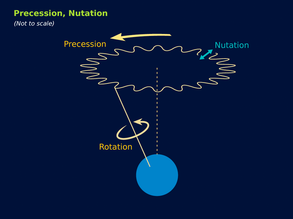
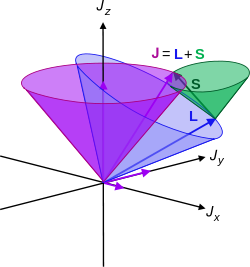
Let me continue the practical example, i.e. the example of the NH₃ molecule, as shown below. We abstracted away from all of its motion, except for its angular momentum – or its spin, you’d like to say, but that’s rather confusing, because we shouldn’t be using that term for the classical situation we’re presenting here – around its axis of symmetry. That angular momentum doesn’t change from state | 1 〉 to state | 2 〉. What’s happening here is that we allow the nitrogen atom to flip through the other side, so it tunnels through the plane of the hydrogen atoms, thereby going through an energy barrier.

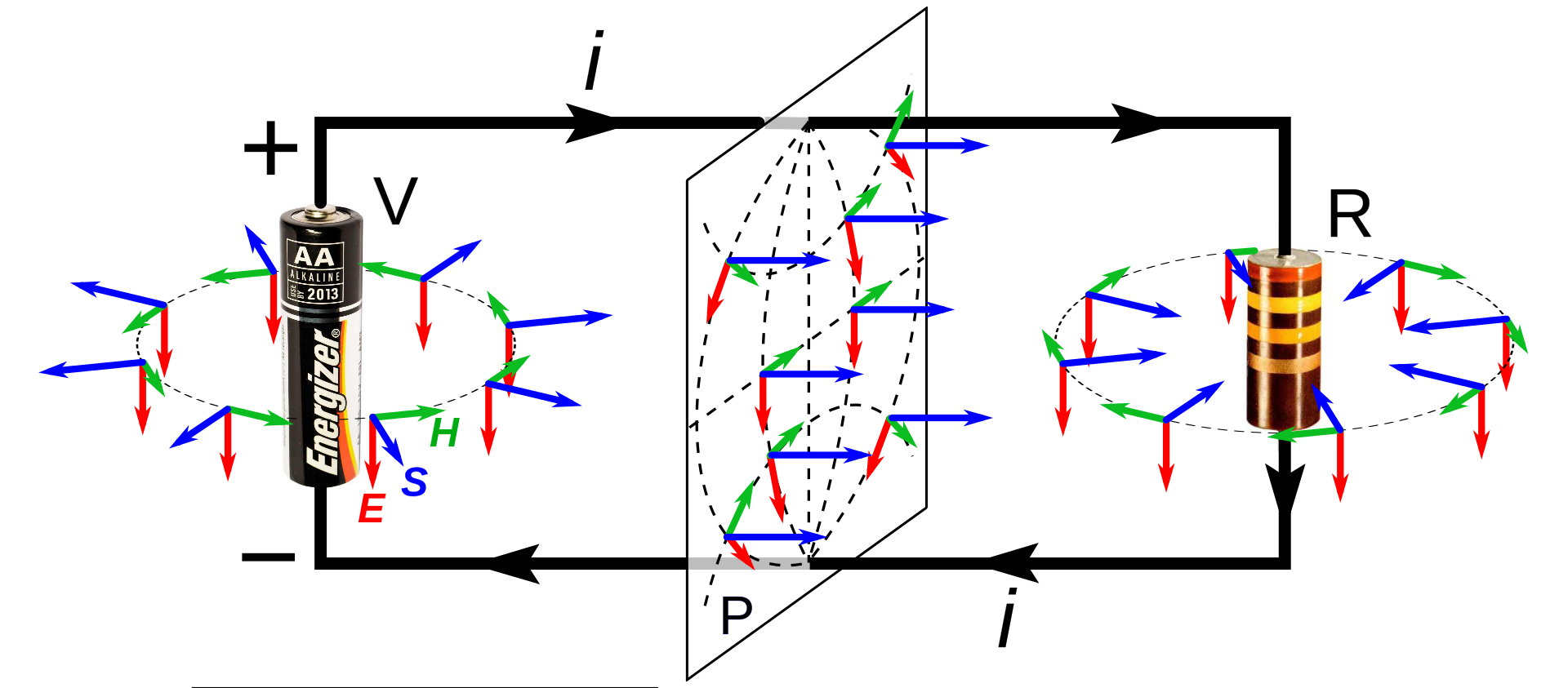
It’s important to note that we do not specify what that energy barrier consists of. In fact, the illustration above may be misleading, because it presents all sorts of things we don’t need right now, like the electric dipole moment, or the center of mass of the molecule, which actually doesn’t change, unlike what’s suggested above. We just put them there to remind you that (a) quantum physics is based on physics – so there’s lots of stuff involved – and (b) because we’ll need that electric dipole moment later. But, as we’re introducing it, note that we’re using the μ symbol for it, which is usually reserved for the magnetic dipole moment, which is what you’d usually associate when thinking about the angular momentum or the spin, both in classical as well as in quantum mechanics. So the direction of rotation of our molecule, as indicated by the arrow around the axis at the bottom, and the μ in the illustration itself, have nothing to do with each other. So now you know. Also, as we’re talking symbols, you should note the use of ε to represent an electric field. We’d usually write the electric dipole moment and the electric field vector as p and E respectively, but so we use that now for linear momentum and energy, and so we borrowed them from our study of magnets. 🙂

The point to note is that, when we’re talking about the ‘up’ or ‘down’ state of our ammonia molecule, you shouldn’t think of it as ‘spin up’ or ‘spin down’. It’s not like that: it’s just the nitrogen atom being beneath or above the plane of the hydrogen atoms, and we define beneath or above assuming the direction of spin actually stays the same!

OK. That should be clear enough. In quantum mechanics, the situation is analyzed by associating two energy levels with the ammonia molecule, E₀+ A and E₀− A, so they are separated by an amount equal to 2A. This pair of energy levels has been confirmed experimentally: they are separated by an energy amount equal to 1×10⁻⁴ eV, so that’s less than a ten-thousandth of the energy of a photon in the visible-light spectrum. Therefore, a molecule that has a transition will emit a photon in the microwave range. The principle of a maser is based on exciting the the NH₃ molecules, and then induce transitions. One can do that by applying an external electric field. The mechanism works pretty much like what we described when discussing the tunneling phenomenon: an external force field will change the energy factor in the wavefunction, by adding potential energy (let’s say an amount equal to U) to the total energy, which usually consists of the internal (E_int) and kinetic (p²/(2m) = m·v) energy only. So now we write a·e^{−i[(E_int+ m·v + U)·t − p∙x]/ħ} instead of a·e^{−i[(E_int+ m·v)·t − p∙x]/ħ}.

Of course, a·e^{−i·(E·t − p∙x)/ħ} is an idealized wavefunction only, or a Platonic wavefunction – as I jokingly referred to it in my previous post. A real wavefunction has to deal with these uncertainties: we don’t know E and p. At best, we have a discrete set of possible values, like E₀+ A and E₀− A in this case. But it might as well be some range, which we denote as ΔE and Δp, and then we need to make some assumption in regard to the probability density function that we’re going to associate with it. But I am getting ahead of myself here. Back to NH₃, i.e. our simple two-state system. Let’s first do some mathematical gymnastics.

Choosing another representation

We have two base states in this system: ‘up’ or ‘down’, which we denoted as base state | 1 〉 and base state | 2 〉 respectively. You’ll also remember we wrote the amplitude to find the molecule in either one of these two states as:

C₁= 〈 1 | ψ 〉 = (1/2)·e^{−(i/ħ)·(E₀− A)·t}+ (1/2)·e^{−(i/ħ)·(E₀+ A)·t}
C₂= 〈 2 | ψ 〉 = (1/2)·e^{−(i/ħ)·(E₀− A)·t}– (1/2)·e^{−(i/ħ)·(E₀+ A)·t}

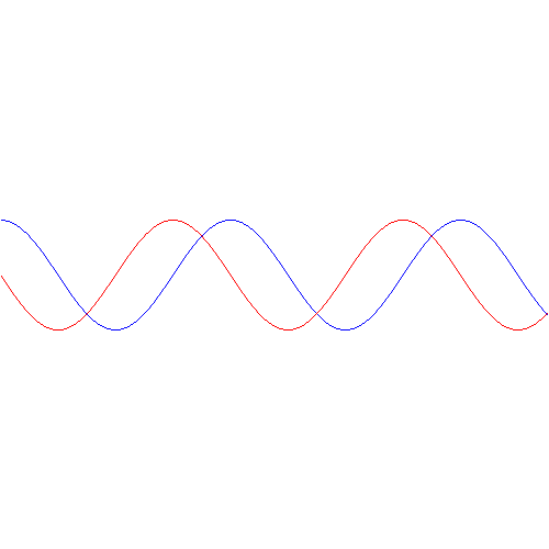
That gave us the following probabilities:

Now, you may think there is only one possible set of base states here, as it’s not like measuring spin along this or that direction. These two base states are much simpler: it’s a matter of the nitrogen being beneath or above the plane of the hydrogens, and we’re only interested in the angular momentum of the molecule around its axis of symmetry to help us define what ‘up’ and what’s ‘down’. That’s all. However, from a quantum math point of view, we can actually choose some other ‘representation’. Now, these base state vectors | i 〉 are a bit tough to understand, so let’s, in our first go at it, use those coefficients C_i, which are ‘proper’ amplitudes. We’ll define two new coefficients, C_I and C_II, which – you’ve guess it – we’ll associate with an alternative set of base states | I 〉 and | II 〉. We’ll define them as follows:

C_I= 〈 I | ψ 〉 = (1/√2)·(C₁− C₂)
C_II= 〈 II | ψ 〉 = (1/√2)·(C₁+ C₂)

[The (1/√2) factor is there because of the normalization condition, obviously. We could take it out and then do the whole analysis to plug it in later, as Feynman does, but I prefer to do it this way, as it reminds us that our wavefunctions are to be related to probabilities at some point in time. :-)]

Now, you can easily check that, when substituting our C₁and C₂for those wavefunctions above, we get:

C_I= 〈 I | ψ 〉 = (1/√2)·e^{−(i/ħ)·(E₀+ A)·t}
C_II= 〈 I | ψ 〉 = (1/√2)·e^{−(i/ħ)·(E₀− A)·t}

Note that the way plus and minus signs switch here makes things not so easy to remember, but that’s how it is. 🙂 So we’ve got our stationary state solutions here, that are associated with probabilities that do not vary in time. [In case you wonder: that’s the definition of a ‘stationary state’: we’ve got something with a definite energy and, therefore, the probability that’s associated with it is some constant.] Of course, now you’ll cry wolf and say: these wavefunctions don’t actually mean anything, do they? They don’t describe how ammonia actually behaves, do they? Well… Yes and no. The base states I and II actually do allow us to describe whatever we need to describe. To be precise, describing the state φ in terms of the base states | 1 〉 and | 2 〉, i.e. writing | φ 〉 as:

| φ 〉 = | 1 〉 C₁ + | 2 〉 C₂,

is mathematically equivalent to writing:

| φ 〉 = | I 〉 C_I + | II 〉 C_II.

We can easily show that, even if it requires some gymnastics indeed—but then you should look at it as just another exercise in quantum math and so, yes, please do go through the logic. First note that the C_I= 〈 I | ψ 〉 = (1/√2)·(C₁− C₂) and C_II= 〈 II | ψ 〉 = (1/√2)·(C₁+ C₂) expressions are equivalent to:

〈 I | ψ 〉 = (1/√2)·[〈 1 | ψ 〉 − 〈 2 | ψ 〉] and 〈 II | ψ 〉 = (1/√2)·[〈 1 | ψ 〉 + 〈 2 | ψ 〉]

Now, using our quantum math rules, we can abstract the | ψ 〉 away, and so we get:

〈 I | = (1/√2)·[〈 1 | − 〈 2 |] and 〈 II | = (1/√2)·[〈 1 | + 〈 2 |]

We could also have applied the complex conjugate rule to the expression for 〈 I | ψ 〉 above (the complex conjugate of a sum (or a product) is the sum (or the product) of the complex conjugates), and then abstract 〈 ψ | away, so as to write:

| I 〉 = (1/√2)·[| 1 〉 − | 2 〉] and | II 〉 = (1/√2)·[| 1 〉 + | 2 〉]

OK. So what? We’ve only shown our new base states can be written as similar combinations as those C_Iand C_IIcoefficients. What proves they are base states? Well… The first rule of quantum math actually defines them as states i respecting the following condition:

〈 i | j〉 = 〈 j | i〉 = δ_ij, with δ_ij= δ_jiis equal to 1 if i = j, and zero if i ≠ j

We can prove that as follows. First, use the | I 〉 = (1/√2)·[| 1 〉 − | 2 〉] and | II 〉 = (1/√2)·[| 1 〉 + | 2 〉] result above to check the following:

〈 I | I 〉 = (1/√2)·[〈 I | 1 〉 − 〈 I | 2 〉]
〈 II | II 〉 = (1/√2)·[〈 II | 1 〉 + 〈 II | 2 〉]
〈 II | I 〉 = (1/√2)·[〈 II | 1 〉 − 〈 II | 2 〉]
〈 I | II 〉 = (1/√2)·[〈 I | 1 〉 + 〈 I | 2 〉]

Now we need to find those 〈 I | i 〉 and 〈 II | i 〉 amplitudes. To do that, we can use that 〈 I | ψ 〉 = (1/√2)·[〈 1 | ψ 〉 − 〈 2 | ψ 〉] and 〈 II | ψ 〉 = (1/√2)·[〈 1 | ψ 〉 + 〈 2 | ψ 〉] equation and substitute:

〈 I | 1 〉 = (1/√2)·[〈 1 | 1 〉 − 〈 2 | 1 〉] = (1/√2)
〈 I | 2 〉 = (1/√2)·[〈 1 | 2 〉 − 〈 2 | 2 〉] = −(1/√2)
〈 II | 1 〉 = (1/√2)·[〈 1 | 1 〉 + 〈 2 | 1 〉] = (1/√2)
〈 II | 2 〉 = (1/√2)·[〈 1 | 2 〉 + 〈 2 | 2 〉] = (1/√2)

So we get:

〈 I | I 〉 = (1/√2)·[〈 I | 1 〉 − 〈 I | 2 〉] = (1/√2)·[(1/√2) + (1/√2)] = (2/(√2·√2) = 1
〈 II | II 〉 = (1/√2)·[〈 II | 1 〉 + 〈 II | 2 〉] = (1/√2)·[(1/√2) + (1/√2)] = 1
〈 II | I 〉 = (1/√2)·[〈 II | 1 〉 − 〈 II | 2 〉] = (1/√2)·[(1/√2) − (1/√2)] = 0
〈 I | II 〉 = (1/√2)·[〈 I | 1 〉 + 〈 I | 2 〉] = (1/√2)·[(1/√2) − (1/√2)] = 0

So… Well.. Yes. That’s equivalent to:

〈 I | I 〉 = 〈 II | II 〉 = 1 and 〈 I | II 〉 = 〈 II | I 〉 = 0

Therefore, we can confidently say that our | I 〉 = (1/√2)·[| 1 〉 − | 2 〉] and | II 〉 = (1/√2)·[| 1 〉 + | 2 〉] state vectors are, effectively, base vectors in their own right. Now, we’re going to have to grow very fond of matrices, so let me write our ‘definition’ of the new base vectors as a matrix formula:

You’ve seen this before. The two-by-two matrix is the transformation matrix for a rotation of state filtering apparatus about the y-axis, over an angle equal to (minus) 90 degrees, when only two states are involved:

You’ll wonder why we should go through all that trouble. Part of it, of course, is to just learn these tricks. The other reason, however, is that it does simplify calculations. Here I need to remind you of the Hamiltonian matrix and the set of differential equations that comes with it. For a system with two base states, we’d have the following set of equations:

Now, adding and subtracting those two equations, and then differentiating the expressions you get (with respect to t), should give you the following two equations:

So what about it? Well… If we transform to the new set of base states, and use the C_Iand C_IIcoefficients instead of those C₁and C₂coefficients, then it turns out that our set of differential equations simplifies, because – as you can see – two out of the four Hamiltonian coefficients are zero, so we can write:

Now you might think that’s not worth the trouble but, of course, now you know how it goes, and so next time it will be easier. 🙂

On a more serious note, I hope you can appreciate the fact that with more states than just two, it will become important to diagonalize the Hamiltonian matrix so as simplify the problem of solving the related set of differential equations. Once we’ve got the solutions, we can always go back to calculate the wavefunctions we want, i.e. the C₁and C₂functions that we happen to like more in this particular case. Just to remind you of how this works, remember that we can describe any state φ both in terms of the base states | 1 〉 and | 2 〉 as well as in terms of the base states | I 〉 and | II 〉, so we can either write:

| φ 〉 = | 1 〉 C₁ + | 2 〉 C₂ or, alternatively, | φ 〉 = | I 〉 C_I + | II 〉 C_II.

Now, if we choose, or define, C_Iand C_IIthe way we do – so that’s as C_I= (1/√2)·(C₁− C₂) and C_II= (1/√2)·(C₁+ C₂) respectively – then the Hamiltonian matrices that come with them are the following ones:

To understand those matrices, let me remind you here of that equation for the Hamiltonian coefficients in those matrices:

U_ij(t + Δt, t) = δ_ij + K_ij(t)·Δt = δ_ij − (i/ħ)·H_ij(t)·Δt

In my humble opinion, this makes the difference clear. The | I 〉 and | II 〉 base states are clearly separated, mathematically, as much as the | 1 〉 and | 2 〉 base states were separated conceptually. There is no amplitude to go from state I to state II, but then both states are a mix of state 1 and 2, so the physical reality they’re describing is exactly the same: we’re just pushing the temporal variation of the probabilities involved from the coefficients we’re using in our differential equations to the base states we use to define those coefficients – or vice versa.

Huh? Yes… I know it’s all quite deep, and I haven’t quite come to terms with it myself, so that’s why I’ll let you think about it. 🙂 To help you think this through, think about this: the C₁ and C₂wavefunctions made sense but, at the same time, they were not very ‘physical’ (read: classical), because they incorporated uncertainty—as they mix two different energy levels. However, the associated base states – which I’ll call ‘up’ and ‘down’ here – made perfect sense, in a classical ‘physical’ sense, that is (my English seems to be getting poorer and poorer—sorry for that!). Indeed, in classical physics, the nitrogen atom is either here or there, right? Not somewhere in-between. 🙂 Now, the C_I and C_IIwavefunctions make sense in the classical sense because they are stationary and, hence, they’re associated with a very definite energy level. In fact, as definite, or as classical, as when we say: the nitrogen atom is either here or there. Not somewhere in-between. But they don’t make sense in some other way: we know that the nitrogen atom will, sooner or later, effectively tunnel through. So they do not describe anything real. So how do we capture reality now? Our C_I and C_IIwavefunctions don’t do that explicitly, but implicitly, as the base states now incorporate all of the uncertainty. Indeed, the C_I and C_IIwavefunctions are described in terms of the base states I and II, which themselves are a mixture of our ‘classical’ up or down states. So, yes, we are kicking the ball around here, from a math point of view. Does that make sense? If not, sorry. I can’t do much more. You’ll just have to think through this yourself. 🙂

Let me just add one little note, totally unrelated to what I just wrote, to conclude this little excursion. I must assume that, in regard of diagonalization, you’ve heard about eigenvalues and eigenvectors. In fact, I must assume you heard about this when you learned about matrices in high school. So… Well… In case you wonder, that’s where we need this stuff. 🙂

OK. On to the next !

The general solution for a two-state system

Now, you’ll wonder why, after all of the talk about the need to simplify the Hamiltonian, I will now present a general solution for any two-state system, i.e. any pair of Hamiltonian equations for two-state systems. However, you’ll soon appreciate why, and you’ll also connect the dots with what I wrote above.

Let me first give you the general solution. In fact, I’ll copy it from Feynman (just click on it to enlarge it, or read it in Feynman’s Lecture on it yourself):

The problem is, of course, how do we interpret that solution? Let me make it big:

This says that the general solution to any two-state system amounts to calculating two separate energy levels using the Hamiltonian coefficients as they are being used in those equations above. So there is an ‘upper’ energy level, which is denoted as E_I, and a ‘lower’ energy level, which is denoted as E_II.

What? So it doesn’t say anything about the Hamiltonian coefficients themselves? No. It doesn’t. What did you expect? Those coefficients define the system as such. So the solution is as general as the ‘two-state system’ we wanted to solve: conceptually, it’s characterized by two different energy levels, but that’s about all we can say about it.

[…] Well… No. The solutions above are specific functional forms and, to find them, we had to make certain assumptions and impose certain conditions so as to ensure there’s any non-zero solution at all! In fact, that’s all the fine print above, so I won’t dwell on that—and you had better stop complaining! 🙂 Having said that, the solutions above are very general indeed, and so now it’s up to us to look at specific two-state systems, like our ammonia molecule, and make educated guesses so as to come up with plausible values or functional forms for those Hamiltonian coefficients. That’s what we did when we equated H₁₁ and H₂₂ with some average energy E₀, and H₁₂ and H₁₂ with some energy A. [Minus A, in fact—but we might have chosen some positive value +A. Same solution. In fact, I wonder why Feynman didn’t go for the +A value. It doesn’t matter, really, because we’re talking energy differences, but… Well… Any case… That’s how it is. I guess he just wanted to avoid having to switch the indices 1 and 2, and the coefficients a and b and what have you. But it’s the same. Honestly. :-)]

So… Well… We could do the same here and analyze the solutions we’ve found in our previous posts but… Well… I don’t think that’s very interesting. In addition, I’ll make some references to that in my next post anyway, where we’re going to be analyzing the ammonia molecule in terms of it I and II states, so as to prepare a full-blown analysis of how a maser works.

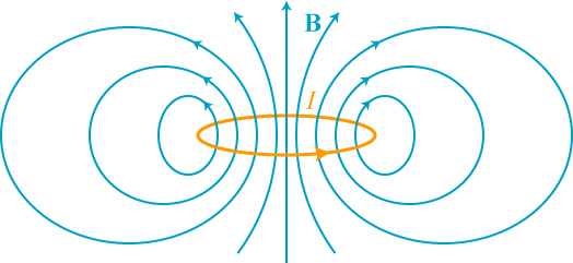
Just to wet your appetite, let me tell you that the mysterious I and II states do have a wonderfully practical physical interpretation as well. Just scroll back it all the way up, and look at the opposite electric dipole moment that’s associated with state 1 and 2. Now, the two pictures have the angular momentum in the same direction, but we might expect that, when looking at a beam of random NH₃ molecules – think of gas being let out of a little jet 🙂 – the angular momentum will be distributed randomly. So… Well… The thing is: the molecules in state I, or in state II, will all have their electric dipole moment lined up in the very same physical direction. So, in that sense, they’re really ‘up’ or ‘down’, and we’ll be able to separate them in an inhomogeneous electric field, just like we were able to separate ‘up’ or ‘down’ electrons, protons or whatever spin-1/2 particles in an inhomogeneous magnetic field.

But so that’s for the next post. I just wanted to tell you that our | I 〉 and | II 〉 base states do make sense. They’re more than just ‘mathematical’ states. They make sense as soon as we’re moving away from an analysis in terms of one NH₃ molecule only because… Well… Are you surprised, really? You shouldn’t be. 🙂 Let’s go for it straight away.

The ammonia molecule in an electric field

Our educating guess of the Hamiltonian matrix for the ammonia molecule was the following:

Hamiltion before

This guess was ‘educated’ because we knew what we wanted to get out of it, and that’s those time-dependent probabilities to be in state 1 or state 2:

Now, we also know that state 1 and 2 are associated with opposite electric dipole moments, as illustrated below.

Hence, it’s only natural, when applying an external electric field ε to a whole bunch of ammonia molecules –think of some beam – that our ‘educated’ guess would change to:

Why the minus sign for με in the H₂₂term? You can answer that question yourself: the associated energy is μ·ε = μ·ε·cosθ, and θ is ±π here, as we’re talking opposite directions. So… There we are. 🙂 The consequences show when using those values in the general solution for our system of differential equations. Indeed, the

equations become:

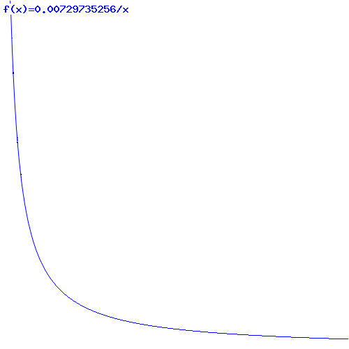
The graph of this looks as follows:

The upshot is: we can separate the the NH₃ molecules in a inhomogeneous electric field based on their state, and then I mean state I or II, not state 1 or 2. How? Let me copy Feynman on that: it’s like a Stern-Gerlach apparatus, really. 🙂

So that’s it. We get the following:

That will feed into the maser, which looks as follows:

But… Well… Analyzing how a maser works involves another realm of physics: cavities and resonances. I don’t want to get into that here. I only wanted to show you why and how different representations of the same thing are useful, and how it translates into a different Hamiltonian matrix. I think I’ve done that, and so let’s call it a night. 🙂 I hope you enjoyed this one. If not… Well… I did. 🙂

Occam’s Razor

The analysis of a two-state system (i.e. the rather famous example of an ammonia molecule ‘flipping’ its spin direction from ‘up’ to ‘down’, or vice versa) in my previous post is a good opportunity to think about Occam’s Razor once more. What are we doing? What does the math tell us?

In the example we chose, we didn’t need to worry about space. It was all about time: an evolving state over time. We also knew the answers we wanted to get: if there is some probability for the system to ‘flip’ from one state to another, we know it will, at some point in time. We also want probabilities to add up to one, so we knew the graph below had to be the result we would find: if our molecule can be in two states only, and it starts of in one, then the probability that it will remain in that state will gradually decline, while the probability that it flips into the other state will gradually increase, which is what is depicted below.

However, the graph above is only a Platonic idea: we don’t bother to actually verify what state the molecule is in. If we did, we’d have to ‘re-set’ our t = 0 point, and start all over again. The wavefunction would collapse, as they say, because we’ve made a measurement. However, having said that, yes, in the physicist’s Platonic world of ideas, the probability functions above make perfect sense. They are beautiful. You should note, for example, that P₁ (i.e. the probability to be in state 1) and P₂ (i.e. the probability to be in state 2) add up to 1 all of the time, so we don’t need to integrate over a cycle or something: so it’s all perfect!

These probability functions are based on ideas that are even more Platonic: interfering amplitudes. Let me explain.

Quantum physics is based on the idea that these probabilities are determined by some wavefunction, a complex-valued amplitude that varies in time and space. It’s a two-dimensional thing, and then it’s not. It’s two-dimensional because it combines a sine and cosine, i.e. a real and an imaginary part, but the argument of the sine and the cosine is the same, and the sine and cosine are the same function, except for a phase shift equal to π. We write:

a·e^−iθ= a·cos(θ) – a·sin(−θ) = a·cosθ – a·sinθ

The minus sign is there because it turns out that Nature measures angles, i.e. our phase, clockwise, rather than counterclockwise, so that’s not as per our mathematical convention. But that’s a minor detail, really. [It should give you some food for thought, though.] For the rest, the related graph is as simple as the formula:

Now, the phase of this wavefunction is written as θ = (ω·t − k ∙x). Hence, ω determines how this wavefunction varies in time, and the wavevector k tells us how this wave varies in space. The young Frenchman Comte Louis de Broglie noted the mathematical similarity between the ω·t − k ∙x expression and Einstein’s four-vector product p_μx_μ= E·t − p∙x, which remains invariant under a Lorentz transformation. He also understood that the Planck-Einstein relation E = ħ·ω actually defines the energy unit and, therefore, that any frequency, any oscillation really, in space or in time, is to be expressed in terms of ħ.

[To be precise, the fundamental quantum of energy is h = ħ·2π, because that’s the energy of one cycle. To illustrate the point, think of the Planck-Einstein relation. It gives us the energy of a photon with frequency f: E_γ = h·f. If we re-write this equation as E_γ/f = h, and we do a dimensional analysis, we get: h = E_γ/f ⇔ 6.626×10⁻³⁴ joule·second = [x joule]/[f cycles per second] ⇔ h = 6.626×10⁻³⁴ joule per cycle. It’s only because we are expressing ω and k as angular frequencies (i.e. in radians per second or per meter, rather than in cycles per second or per meter) that we have to think of ħ = h/2π rather than h.]

Louis de Broglie connected the dots between some other equations too. He was fully familiar with the equations determining the phase and group velocity of composite waves, or a wavetrain that actually might represent a wavicle traveling through spacetime. In short, he boldly equated ω with ω = E/ħ and k with k = p/ħ, and all came out alright. It made perfect sense!

I’ve written enough about this. What I want to write about here is how this also makes for the situation on hand: a simple two-state system that depends on time only. So its phase is θ = ω·t = E₀/ħ. What’s E₀? It is the total energy of the system, including the equivalent energy of the particle’s rest mass and any potential energy that may be there because of the presence of one or the other force field. What about kinetic energy? Well… We said it: in this case, there is no translational or linear momentum, so p = 0. So our Platonic wavefunction reduces to:

a·e^−iθ= ae⁻⁽^{i/ħ)·(E₀·t)}

Great! […] But… Well… No! The problem with this wavefunction is that it yields a constant probability. To be precise, when we take the absolute square of this wavefunction – which is what we do when calculating a probability from a wavefunction − we get P = a², always. The ‘normalization’ condition (so that’s the condition that probabilities have to add up to one) implies that P₁ = P₂ = a² = 1/2. Makes sense, you’ll say, but the problem is that this doesn’t reflect reality: these probabilities do not evolve over time and, hence, our ammonia molecule never ‘flips’ its spin direction from ‘up’ to ‘down’, or vice versa. In short, our wavefunction does not explain reality.

The problem is not unlike the problem we’d had with a similar function relating the momentum and the position of a particle. You’ll remember it: we wrote it as a·e^−iθ= ae⁽^{i/ħ)·(p·x)}. [Note that we can write a·e^−iθ= a·e⁻⁽^{i/ħ)·(E₀·t − p·x)}= a·e⁻⁽ⁱ^/ħ)·(E^₀·t)·e⁽^{i/ħ)·(p·x)}, so we can always split our wavefunction in a ‘time’ and a ‘space’ part.] But then we found that this wavefunction also yielded a constant and equal probability all over space, which implies our particle is everywhere (and, therefore, nowhere, really).

In quantum physics, this problem is solved by introducing uncertainty. Introducing some uncertainty about the energy, or about the momentum, is mathematically equivalent to saying that we’re actually looking at a composite wave, i.e. the sum of a finite or infinite set of component waves. So we have the same ω = E/ħ and k = p/ħ relations, but we apply them to n energy levels, or to some continuous range of energy levels ΔE. It amounts to saying that our wave function doesn’t have a specific frequency: it now has n frequencies, or a range of frequencies Δω = ΔE/ħ.

We know what that does: it ensures our wavefunction is being ‘contained’ in some ‘envelope’. It becomes a wavetrain, or a kind of beat note, as illustrated below:

[The animation also shows the difference between the group and phase velocity: the green dot shows the group velocity, while the red dot travels at the phase velocity.]

This begs the following question: what’s the uncertainty really? Is it an uncertainty in the energy, or is it an uncertainty in the wavefunction? I mean: we have a function relating the energy to a frequency. Introducing some uncertainty about the energy is mathematically equivalent to introducing uncertainty about the frequency. Of course, the answer is: the uncertainty is in both, so it’s in the frequency and in the energy and both are related through the wavefunction. So… Well… Yes. In some way, we’re chasing our own tail. 🙂

However, the trick does the job, and perfectly so. Let me summarize what we did in the previous post: we had the ammonia molecule, i.e. an NH₃ molecule, with the nitrogen ‘flipping’ across the hydrogens from time to time, as illustrated below:

This ‘flip’ requires energy, which is why we associate two energy levels with the molecule, rather than just one. We wrote these two energy levels as E₀+ A and E₀− A. That assumption solved all of our problems. [Note that we don’t specify what the energy barrier really consists of: moving the center of mass obviously requires some energy, but it is likely that a ‘flip’ also involves overcoming some electrostatic forces, as shown by the reversal of the electric dipole moment in the illustration above.] To be specific, it gave us the following wavefunctions for the amplitude to be in the ‘up’ or ‘1’ state versus the ‘down’ or ‘2’ state respectivelly:

C₁= (1/2)·e^{−(i/ħ)·(E₀− A)·t}+ (1/2)·e^{−(i/ħ)·(E₀+ A)·t}
C₂= (1/2)·e^{−(i/ħ)·(E₀− A)·t}– (1/2)·e^{−(i/ħ)·(E₀+ A)·t}

Both are composite waves. To be precise, they are the sum of two component waves with a temporal frequency equal to ω₁= (E₀− A)/ħ and ω₁= (E₀+ A)/ħ respectively. [As for the minus sign in front of the second term in the wave equation for C₂, −1 = e^±iπ, so + (1/2)·e^{−(i/ħ)·(E₀+ A)·t}and – (1/2)·e^{−(i/ħ)·(E₀+ A)·t} are the same wavefunction: they only differ because their relative phase is shifted by ±π.] So the so-called base states of the molecule themselves are associated with two different energy levels: it’s not like one state has more energy than the other.

You’ll say: so what?

Well… Nothing. That’s it really. That’s all I wanted to say here. The absolute square of those two wavefunctions gives us those time-dependent probabilities above, i.e. the graph we started this post with. So… Well… Done!

You’ll say: where’s the ‘envelope’? Oh! Yes! Let me tell you. The C₁(t) and C₂(t) equations can be re-written as:

Now, remembering our rules for adding and subtracting complex conjugates (e^iθ + e^–iθ = 2cosθ and e^iθ − e^–iθ = 2sinθ), we can re-write this as:

So there we are! We’ve got wave equations whose temporal variation is basically defined by E₀but, on top of that, we have an envelope here: the cos(A·t/ħ) and sin(A·t/ħ) factor respectively. So their magnitude is no longer time-independent: both the phase as well as the amplitude now vary with time. The associated probabilities are the ones we plotted:

|C₁(t)|²= cos²[(A/ħ)·t], and
|C₂(t)|²= sin²[(A/ħ)·t].

So, to summarize it all once more, allowing the nitrogen atom to push its way through the three hydrogens, so as to flip to the other side, thereby breaking the energy barrier, is equivalent to associating two energy levels to the ammonia molecule as a whole, thereby introducing some uncertainty, or indefiniteness as to its energy, and that, in turn, gives us the amplitudes and probabilities that we’ve just calculated. [And you may want to note here that the probabilities “sloshing back and forth”, or “dumping into each other” – as Feynman puts it – is the result of the varying magnitudes of our amplitudes, so that’s the ‘envelope’ effect. It’s only because the magnitudes vary in time that their absolute square, i.e. the associated probability, varies too.

So… Well… That’s it. I think this and all of the previous posts served as a nice introduction to quantum physics. More in particular, I hope this post made you appreciate the mathematical framework is not as horrendous as it often seems to be.

When thinking about it, it’s actually all quite straightforward, and it surely respects Occam’s principle of parsimony in philosophical and scientific thought, also know as Occam’s Razor: “When trying to explain something, it is vain to do with more what can be done with less.” So the math we need is the math we need, really: nothing more, nothing less. As I’ve said a couple of times already, Occam would have loved the math behind QM: the physics call for the math, and the math becomes the physics.

That’s what makes it beautiful. 🙂

Post scriptum:

One might think that the addition of a term in the argument in itself would lead to a beat note and, hence, a varying probability but, no! We may look at e^{−(i/ħ)·(E₀+ A)·t}as a product of two amplitudes:

e^{−(i/ħ)·(E₀+ A)·t}= e^{−(i/ħ)·E₀·t}·e^{−(i/ħ)·A·t}

But, when writing this all out, one just gets a cos(α·t+β·t)–sin(α·t+β·t), whose absolute square |cos(α·t+β·t)–sin(α·t+β·t)|²= 1. However, writing e^{−(i/ħ)·(E₀+ A)·t}as a product of two amplitudes in itself is interesting. We multiply amplitudes when an event consists of two sub-events. For example, the amplitude for some particle to go from s to x via some point a is written as:

〈 x | s 〉_{via a} = 〈 x | a 〉〈 a | s 〉

Having said that, the graph of the product is uninteresting: the real and imaginary part of the wavefunction are a simple sine and cosine function, and their absolute square is constant, as shown below.

Adding two waves with very different frequencies – A is a fraction of E₀– gives a much more interesting pattern, like the one below, which shows an e^−iαt+e^−iβt= cos(αt)−i·sin(αt)+cos(βt)−i·sin(βt) = cos(αt)+cos(βt)−i·[sin(αt)+sin(βt)] pattern for α = 1 and β = 0.1.

That doesn’t look a beat note, does it? The graphs below, which use 0.5 and 0.01 for β respectively, are not typical beat notes either.

We get our typical ‘beat note’ only when we’re looking at a wave traveling in space, so then we involve the space variable x again, and the relations that come with in, i.e. a phase velocity v_p= ω/k = (E/ħ)/(p/ħ) = E/p = c²/v (read: all component waves travel at the same speed), and a group velocity v_g= dω/dk = v (read: the composite wave or wavetrain travels at the classical speed of our particle, so it travels with the particle, so to speak). That’s what’s I’ve shown numerous times already, but I’ll insert one more animation here, just to make sure you see what we’re talking about. [Credit for the animation goes to another site, one on acoustics, actually!]

So what’s left? Nothing much. The only thing you may want to do is to continue thinking about that wavefunction. It’s tempting to think it actually is the particle, somehow. But it isn’t. So what is it then? Well… Nobody knows, really, but I like to think it does travel with the particle. So it’s like a fundamental property of the particle. We need it every time when we try to measure something: its position, its momentum, its spin (i.e. angular momentum) or, in the example of our ammonia molecule, its orientation in space. So the funny thing is that, in quantum mechanics,

We can measure probabilities only, so there’s always some randomness. That’s how Nature works: we don’t really know what’s happening. We don’t know the internal wheels and gears, so to speak, or the ‘hidden variables’, as one interpretation of quantum mechanics would say. In fact, the most commonly accepted interpretation of quantum mechanics says there are no ‘hidden variables’.
But then, as Polonius famously put, there is a method in this madness, and the pioneers – I mean Werner Heisenberg, Louis de Broglie, Niels Bohr, Paul Dirac, etcetera – discovered. All probabilities can be found by taking the square of the absolute value of a complex-valued wavefunction (often denoted by Ψ), whose argument, or phase (θ), is given by the de Broglie relations ω = E/ħ and k = p/ħ:

θ = (ω·t − k ∙x) = (E/ħ)·t − (p/ħ)·x

That should be obvious by now, as I’ve written dozens of posts on this by now. 🙂 I still have trouble interpreting this, however—and I am not ashamed, because the Great Ones I just mentioned have trouble with that too. But let’s try to go as far as we can by making a few remarks:

Adding two terms in math implies the two terms should have the same dimension: we can only add apples to apples, and oranges to oranges. We shouldn’t mix them. Now, the (E/ħ)·t and (p/ħ)·x terms are actually dimensionless: they are pure numbers. So that’s even better. Just check it: energy is expressed in newton·meter (force over distance, remember?) or electronvolts (1 eV = 1.6×10⁻¹⁹J = 1.6×10⁻¹⁹N·m); Planck’s constant, as the quantum of action, is expressed in J·s or eV·s; and the unit of (linear) momentum is 1 N·s = 1 kg·m/s = 1 N·s. E/ħ gives a number expressed per second, and p/ħ a number expressed per meter. Therefore, multiplying it by t and x respectively gives us a dimensionless number indeed.
It’s also an invariant number, which means we’ll always get the same value for it. As mentioned above, that’s because the four-vector product p_μx_μ= E·t − p∙x is invariant: it doesn’t change when analyzing a phenomenon in one reference frame (e.g. our inertial reference frame) or another (i.e. in a moving frame).
Now, Planck’s quantum of action h or ħ (they only differ in their dimension: h is measured in cycles per second and ħ is measured in radians per second) is the quantum of energy really. Indeed, if “energy is the currency of the Universe”, and it’s real and/or virtual photons who are exchanging it, then it’s good to know the currency unit is h, i.e. the energy that’s associated with one cycle of a photon.
It’s not only time and space that are related, as evidenced by the fact that t − x itself is an invariant four-vector, E and p are related too, of course! They are related through the classical velocity of the particle that we’re looking at: E/p = c²/v and, therefore, we can write: E·β = p·c, with β = v/c, i.e. the relative velocity of our particle, as measured as a ratio of the speed of light. Now, I should add that the t − x four-vector is invariant only if we measure time and space in equivalent units. Otherwise, we have to write c·t − x. If we do that, so our unit of distance becomes c meter, rather than one meter, or our unit of time becomes the time that is needed for light to travel one meter, then c = 1, and the E·β = p·c becomes E·β = p, which we also write as β = p/E: the ratio of the energy and the momentum of our particle is its (relative) velocity.

θ = (ω·t − k ∙x) = E·t − p·x

Now, θ is the argument of a wavefunction, and we can always re-scale such argument by multiplying or dividing it by some constant. It’s just like writing the argument of a wavefunction as v·t–x or (v·t–x)/v = t –x/v with v the velocity of the waveform that we happen to be looking at. [In case you have trouble following this argument, please check the post I did for my kids on waves and wavefunctions.] Now, the energy conservation principle tells us the energy of a free particle won’t change. [Just to remind you, a ‘free particle’ means it is present in a ‘field-free’ space, so our particle is in a region of uniform potential.] You see what I am going to do now: we can, in this case, treat E as a constant, and divide E·t − p·x by E, so we get a re-scaled phase for our wavefunction, which I’ll write as:

φ = (E·t − p·x)/E = t − (p/E)·x = t − β·x

Now that’s the argument of a wavefunction with the argument expressed in distance units. Alternatively, we could also look at p as some constant, as there is no variation in potential energy that will cause a change in momentum, i.e. in kinetic energy. We’d then divide by p and we’d get (E·t − p·x)/p = (E/p)·t − x) = t/β − x, which amounts to the same, as we can always re-scale by multiplying it with β, which would then yield the same t − β·x argument.

Φ(φ) = a·e^−iφ= a·e^{−i(t − β·x)}

Of course, the analysis above does not include uncertainty. Our information on the energy and the momentum of our particle will be incomplete: we’ll write E = E₀± σ_E, and p = p₀± σ_p. [I am a bit tired of using the Δ symbol, so I am using the σ symbol here, which denotes a standard deviation of some density function. It underlines the probabilistic, or statistical, nature of our approach.] But, including that, we’ve pretty much explained what quantum physics is about here.

You just need to get used to that complex exponential: e^−iφ = cos(−φ) + i·sin(−φ) = cos(φ) − i·sin(φ). Of course, it would have been nice if Nature would have given us a simple sine or cosine function. [Remember the sine and cosine function are actually the same, except for a phase difference of 90 degrees: sin(φ) = cos(π/2−φ) = cos(φ+π/2). So we can go always from one to the other by shifting the origin of our axis.] But… Well… As we’ve shown so many times already, a real-valued wavefunction doesn’t explain the interference we observe, be it interference of electrons or whatever other particles or, for that matter, the interference of electromagnetic waves itself, which, as you know, we also need to look at as a stream of photons , i.e. light quanta, rather than as some kind of infinitely flexible aether that’s undulating, like water or air.

So… Well… Just accept that e^−iφ is a very simple periodic function, consisting of two sine waves rather than just one, as illustrated below.

And then you need to think of stuff like this (the animation is taken from Wikipedia), but then with a projection of the sine of those phasors too. It’s all great fun, so I’ll let you play with it now. 🙂

The Hamiltonian for a two-state system: the ammonia example

Ammonia, i.e. NH₃, is a colorless gas with a strong smell. Its serves as a precursor in the production of fertilizer, but we also know it as a cleaning product, ammonium hydroxide, which is NH₃ dissolved in water. It has a lot of other uses too. For example, its use in this post, is to illustrate a two-state system. 🙂 We’ll apply everything we learned in our previous posts and, as I mentioned when finishing the last of those rather mathematical pieces, I think the example really feels like a reward after all of the tough work on all of those abstract concepts – like that Hamiltonian matrix indeed – so I hope you enjoy it. So… Here we go!

The geometry of the NH₃ molecule can be described by thinking of it as a trigonal pyramid, with the nitrogen atom (N) at its apex, and the three hydrogen atoms (H) at the base, as illustrated below. [Feynman’s illustration is slightly misleading, though, because it may give the impression that the hydrogen atoms are bonded together somehow. That’s not the case: the hydrogen atoms share their electron with the nitrogen, thereby completing the outer shell of both atoms. This is referred to as a covalent bond. You may want to look it up, but it is of no particular relevance to what follows here.]

Here, we will only worry about the spin of the molecule about its axis of symmetry, as shown above, which is either in one direction or in the other, obviously. So we’ll discuss the molecule as a two-state system. So we don’t care about its translational (i.e. linear) momentum, its internal vibrations, or whatever else that might be going on. It is one of those situations illustrating that the spin vector, i.e. the vector representing angular momentum, is an axial vector: the first state, which is denoted by | 1 〉 is not the mirror image of state | 2 〉. In fact, there is a more sophisticated version of the illustration above, which usefully reminds us of the physics involved.

It should be noted, however, that we don’t need to specify what the energy barrier really consists of: moving the center of mass obviously requires some energy, but it is likely that a ‘flip’ also involves overcoming some electrostatic forces, as shown by the reversal of the electric dipole moment in the illustration above. In fact, the illustration may confuse you, because we’re usually thinking about some net electric charge that’s spinning, and so the angular momentum results in a magnetic dipole moment, that’s either ‘up’ or ‘down’, and it’s usually also denoted by the very same μ symbol that’s used below. As I explained in my post on angular momentum and the magnetic moment, it’s related to the angular momentum J through the so-called g-number. In the illustration above, however, the μ symbol is used to denote an electric dipole moment, so that’s different. Don’t rack your brain over it: just accept there’s an energy barrier, and it requires energy to get through it. Don’t worry about its details!

Indeed, in quantum mechanics, we abstract away from such nitty-gritty, and so we just say that we have base states | i 〉 here, with i equal to 1 or 2. One or the other. Now, in our post on quantum math, we introduced what Feynman only half-jokingly refers to as the Great Law of Quantum Physics: | = ∑ | i 〉〈 i | over all base states i. It basically means that we should always describe our initial and end states in terms of base states. Applying that principle to the state of our ammonia molecule, which we’ll denote by | ψ 〉, we can write:

You may – in fact, you should – mechanically apply that | = ∑ | i 〉〈 i | substitution to | ψ 〉 to get what you get here, but you should also think about what you’re writing. It’s not an easy thing to interpret, but it may help you to think of the similarity of the formula above with the description of a vector in terms of its base vectors, which we write as A = A_x·e₁+ A_y·e₂ + A_z·e₃. Just substitute the A_icoefficients for C_i and the e_ibase vectors for the | i 〉 base states, and you may understand this formula somewhat better. It also explains why the | ψ 〉 state is often referred to as the | ψ 〉 state vector: unlike our A = ∑ A_i·e_isum of base vectors, our | 1 〉 C₁ + | 2 〉 C₂sum does not have any geometrical interpretation but… Well… Not all ‘vectors’ in math have a geometric interpretation, and so this is a case in point.

It may also help you to think of the time-dependency. Indeed, this formula makes a lot more sense when realizing that the state of our ammonia molecule, and those coefficients C_i, depend on time, so we write: ψ = ψ(t) and C_i= C_i(t). Hence, if we would know, for sure, that our molecule is always in state | 1 〉, then C₁ = 1 and C₂ = 0, and we’d write: | ψ 〉 = | 1 〉 = | 1 〉 1 + | 2 〉 0. [I am always tempted to insert a little dot (·), and change the order of the factors, so as to show we’re talking some kind of product indeed – so I am tempted to write | ψ 〉 = C₁·| 1 〉 C₁ + C₂·| 2 〉 C₂, but I note that’s not done conventionally, so I won’t do it either.]

Why this time dependency? It’s because we’ll allow for the possibility of the nitrogen to push its way through the pyramid – through the three hydrogens, really – and flip to the other side. It’s unlikely, because it requires a lot of energy to get half-way through (we’ve got what we referred to as an energy barrier here), but it may happen and, as we’ll see shortly, it results in us having to think of the the ammonia molecule as having two separate energy levels, rather than just one. We’ll denote those energy levels as E₀ ± A. However, I am getting ahead of myself here, so let me get back to the main story.

To fully understand the story, you should really read my previous post on the Hamiltonian, which explains how those C_i coefficients, as a function of time, can be determined. They’re determined by a set of differential equations (i.e. equations involving a function and the derivative of that function) which we wrote as:

If we have two base states only – which is the case here – then this set of equations is:

Two equations and two functions – C₁= C₁(t) and C₂= C₂(t) – so we should be able to solve this thing, right? Well… No. We don’t know those H_ijcoefficients. As I explained in my previous post, they also evolve in time, so we should write them as H_ij(t) instead of H_ijtout court, and so it messes the whole thing up. We have two equations and six functions really. There is no way we can solve this! So how do we get out of this mess?

Well… By trial and error, I guess. 🙂 Let us just assume the molecule would behave nicely—which we know it doesn’t, but so let’s push the ‘classical’ analysis as far as we can, so we might get some clues as to how to solve this problem. In fact, our analysis isn’t ‘classical’ at all, because we’re still talking amplitudes here! However, you’ll agree the ‘simple’ solution would be that our ammonia molecule doesn’t ‘tunnel’. It just stays in the same spin direction forever. Then H₁₂and H₂₁must be zero (think of the U₁₂(t + Δt, t) and U₂₁(t + Δt, t) functions) and H₁₁and H₂₂are equal to… Well… I’d love to say they’re equal to 1 but… Well… You should go through my previous posts: these Hamiltonian coefficients are related to probabilities but… Well… Same-same but different, as they say in Asia. 🙂 They’re amplitudes, which are things you use to calculate probabilities. But calculating probabilities involve normalization and other stuff, like allowing for interference of amplitudes, and so… Well… To make a long story short, if our ammonia molecule would stay in the same spin direction forever, then H₁₁and H₂₂are not one but some constant. In any case, the point is that they would not change in time (so H₁₁(t) = H₁₁ and H₂₂(t ) = H₂₂), and, therefore, our two equations would reduce to:

So the coefficients are now proper coefficients, in the sense that they’ve got some definite value, and so we have two equations and two functions only now, and so we can solve this. Indeed, remembering all of the stuff we wrote on the magic of exponential functions (more in particular, remembering that d[e^x]/dx), we can understand the proposed solution:

As Feynman notes: “These are just the amplitudes for stationary states with the energies E₁= H₁₁ and E₂= H₂₂.” Now let’s think about that. Indeed, I find the term ‘stationary’ state quite confusing, as it’s ill-defined. In this context, it basically means that we have a wavefunction that is determined by (i) a definite (i.e. unambiguous, or precise) energy level and (ii) that there is no spatial variation. Let me refer you to my post on the basics of quantum math here. We often use a sort of ‘Platonic’ example of the wavefunction indeed:

a·e^−i·θ= e^{−i·(ω·t − k ∙x)} = a·e^{−(i/ħ)·(E·t − p∙x)}

So that’s a wavefunction assuming the particle we’re looking at has some well-defined energy E and some equally well-defined momentum p. Now, that’s kind of ‘Platonic’ indeed, because it’s more like an idea, rather than something real. Indeed, a wavefunction like that means that the particle is everywhere and nowhere, really—because its wavefunction is spread out all of over space. Of course, we may think of the ‘space’ as some kind of confined space, like a box, and then we can think of this particle as being ‘somewhere’ in that box, and then we look at the temporal variation of this function only – which is what we’re doing now: we don’t consider the space variable x at all. So then the equation reduces to a·e^{–(i/ħ)·(E·t)}, and so… Well… Yes. We do find that our Hamiltonian coefficient H_iiis like the energy of the | i 〉 state of our NH₃ molecule, so we write: H₁₁= E₁, and H₂₂= E₂, and the ‘wavefunctions’ of our C₁and C₂coefficients can be written as:

C₁= a·e^{−(i/ħ)·(H₁₁·t)}= a·e^{−(i/ħ)·(E₁·t)}, with H₁₁= E₁, and
C₂= a·e^{−(i/ħ)·(H₂₂·t)}= a·e^{−(i/ħ)·(E₂·t)}, with H₂₂= E₂.

But can we interpret C₁and C₂as proper amplitudes? They are just coefficients in these equations, aren’t they? Well… Yes and no. From what we wrote in previous posts, you should remember that these C_icoefficients are equal to 〈 i | ψ 〉, so they are the amplitude to find our ammonia molecule in one state or the other.

Back to Feynman now. He adds, logically but brilliantly:

“We note, however, that for the ammonia molecule the two states |1〉 and |2〉 have a definite symmetry. If nature is at all reasonable, the matrix elements H₁₁ and H₂₂ must be equal. We’ll call them both E₀, because they correspond to the energy the states would have if H₁₁ and H₂₂ were zero.”

So our C₁and C₂amplitudes then reduce to:

C₁= 〈 1 | ψ 〉 = a·e^{−(i/ħ)·(E₀·t)}
C₂=〈 2 | ψ 〉 = a·e^{−(i/ħ)·(E₀·t)}

We can now take the absolute square of both to find the probability for the molecule to be in state 1 or in state 2:

|〈 1 | ψ 〉|²= |a·e^{−(i/ħ)·(E₀·t)}|²= a²
|〈 2 | ψ 〉|²= |a·e^{−(i/ħ)·(E₀·t)}|²= a²

Now, the probabilities have to add up to 1, so a²+ a²= 1 and, therefore, the probability to be in either in state 1 or state 2 is 0.5, which is what we’d expect.

Note: At this point, it is probably good to get back to our | ψ 〉 = | 1 〉 C₁ + | 2 〉 C₂equation, so as to try to understand what it really says. Substituting the a·e^{−(i/ħ)·(E₀·t)} expression for C₁ and C₂yields:

| ψ 〉 = | 1 〉 a·e^{−(i/ħ)·(E₀·t)} + | 2 〉 a·e^{−(i/ħ)·(E₀·t)}= [| 1 〉 + | 2 〉] a·e^{−(i/ħ)·(E₀·t)}

Now, what is this saying, really? In our previous post, we explained this is an ‘open’ equation, so it actually doesn’t mean all that much: we need to ‘close’ or ‘complete’ it by adding a ‘bra’, i.e. a state like 〈 χ |, so we get a 〈 χ | ψ〉 type of amplitude that we can actually do something with. Now, in this case, our final 〈 χ | state is either 〈 1 | or 〈 2 |, so we write:

〈 1 | ψ 〉 = [〈 1 | 1 〉 + 〈 1 | 2 〉]·a·e^{−(i/ħ)·(E₀·t)}= [1 + 0]·a·e^{−(i/ħ)·(E₀·t)}· = a·e^{−(i/ħ)·(E₀·t)}
〈 2 | ψ 〉 = [〈 2 | 1 〉 + 〈 2 | 2 〉]·a·e^{−(i/ħ)·(E₀·t)}= [0 + 1]·a·e^{−(i/ħ)·(E₀·t)}· = a·e^{−(i/ħ)·(E₀·t)}

Note that I finally added the multiplication dot (·) because we’re talking proper amplitudes now and, therefore, we’ve got a proper product too: we multiply one complex number with another. We can now take the absolute square of both to find the probability for the molecule to be in state 1 or in state 2:

|〈 1 | ψ 〉|²= |a·e^{−(i/ħ)·(E₀·t)}|²= a²
|〈 2 | ψ 〉|²= |a·e^{−(i/ħ)·(E₀·t)}|²= a²

Unsurprisingly, we find the same thing: these probabilities have to add up to 1, so a²+ a²= 1 and, therefore, the probability to be in state 1 or state 2 is 0.5. So the notation and the logic behind makes perfect sense. But let me get back to the lesson now.

The point is: the true meaning of a ‘stationary’ state here, is that we have non-fluctuating probabilities. So they are and remain equal to some constant, i.e. 1/2 in this case. This implies that the state of the molecule does not change: there is no way to go from state 1 to state 2 and vice versa. Indeed, if we know the molecule is in state 1, it will stay in that state. [Think about what normalization of probabilities means when we’re looking at one state only.]

You should note that these non-varying probabilities are related to the fact that the amplitudes have a non-varying magnitude. The phase of these amplitudes varies in time, of course, but their magnitude is and remains a, always. The amplitude is not being ‘enveloped’ by another curve, so to speak.

OK. That should be clear enough. Sorry I spent so much time on this, but this stuff on ‘stationary’ states comes back again and again and so I just wanted to clear that up as much as I can. Let’s get back to the story.

So we know that, what we’re describing above, is not what ammonia does really. As Feynman puts it: “The equations [i.e. the C₁and C₂equations above] don’t tell us what what ammonia really does. It turns out that it is possible for the nitrogen to push its way through the three hydrogens and flip to the other side. It is quite difficult; to get half-way through requires a lot of energy. How can it get through if it hasn’t got enough energy? There is some amplitude that it will penetrate the energy barrier. It is possible in quantum mechanics to sneak quickly across a region which is illegal energetically. There is, therefore, some [small] amplitude that a molecule which starts in |1〉 will get to the state |2〉. The coefficients H₁₂ and H₂₁ are not really zero.”

He adds: “Again, by symmetry, they should both be the same—at least in magnitude. In fact, we already know that, in general, H_ijmust be equal to the complex conjugate of H_ji.”

His next step, then, is to interpreted as either a stroke of genius or, else, as unexplained. 🙂 He invokes the symmetry of the situation to boldly state that H₁₂is some real negative number, which he denotes as −A, which – because it’s a real number (so the imaginary part is zero) – must be equal to its complex conjugate H₂₁. So then Feynman does this fantastic jump in logic. First, he keeps using the E₀ value for H₁₁ and H₂₂, motivating that as follows: “If nature is at all reasonable, the matrix elements H₁₁ and H₂₂ must be equal, and we’ll call them both E₀, because they correspond to the energy the states would have if H₁₁ and H₂₂ were zero.” Second, he uses that minus A value for H₁₂and H₂₁. In short, the two equations and six functions are now reduced to:

Solving these equations is rather boring. Feynman does it as follows:

solution

Now, what does these equations actually mean? It depends on those a and b coefficients. Looking at the solutions, the most obvious question to ask is: what if a or b are zero? If b is zero, then the second terms in both equations is zero, and so C₁ and C₂ are exactly the same: two amplitudes with the same temporal frequency ω = (E₀− A)/ħ. If a is zero, then C₁ and C₂ are the same too, but with opposite sign: two amplitudes with the same temporal frequency ω = (E₀+ A)/ħ. Squaring them – in both cases (i.e. for a = 0 or b = 0) – yields, once again, an equal and constant probability for the spin of the ammonia molecule to in the ‘up’ or ‘down’ or ‘down’. To be precise, we We can now take the absolute square of both to find the probability for the molecule to be in state 1 or in state 2:

For b = 0: |〈 1 | ψ 〉|²= |(a/2)·e^{−(i/ħ)·(E₀− A)·t}|²= a²/4 = |〈 2 | ψ 〉|²
For a = 0: |〈 1 | ψ 〉|²=|(b/2)·e^{−(i/ħ)·(E₀+ A)·t}|²= b²/4 = |〈 2 | ψ 〉|²(the minus sign in front of b/2 is squared away)

So we get two stationary states now. Why two instead of one? Well… You need to use your imagination a bit here. They actually reflect each other: they’re the same as the one stationary state we found when assuming our nitrogen atom could not ‘flip’ from one position to the other. It’s just that the introduction of that possibility now results in a sort of ‘doublet’ of energy levels. But so we shouldn’t waste our time on this, as we want to analyze the general case, for which the probabilities to be in state 1 or state 2 do vary in time. So that’s when a and b are non-zero.

To analyze it all, we may want to start with equating t to zero. We then get:

This leads us to conclude that a = b = 1, so our equations for C₁(t) and C₂(t) can now be written as:

Remembering our rules for adding and subtracting complex conjugates (e^iθ + e^–iθ = 2cosθ and e^iθ − e^–iθ = 2sinθ), we can re-write this as:

Now these amplitudes are much more interesting. Their temporal variation is defined by E₀but, on top of that, we have an envelope here: the cos(A·t/ħ) and sin(A·t/ħ) factor respectively. So their magnitude is no longer time-independent: both the phase as well as the amplitude now vary with time. What’s going on here becomes quite obvious when calculating and plotting the associated probabilities, which are

|C₁(t)|²= cos²(A·t/ħ), and
|C₂(t)|²= sin²(A·t/ħ)

respectively (note that the absolute square of i is equal to 1, not −1). The graph of these functions is depicted below.

As Feynman puts it: “The probability sloshes back and forth.” Indeed, the way to think about this is that, if our ammonia molecule is in state 1, then it will not stay in that state. In fact, one can be sure the nitrogen atom is going to flip at some point in time, with the probabilities being defined by that fluctuating probability density function above. Indeed, as time goes by, the probability to be in state 2 increases, until it will effectively be in state 2. And then the cycle reverses.

Our | ψ 〉 = | 1 〉 C₁ + | 2 〉 C₂equation is a lot more interesting now, as we do have a proper mix of pure states now: we never really know in what state our molecule will be, as we have these ‘oscillating’ probabilities now, which we should interpret carefully.

The point to note is that the a = 0 and b = 0 solutions came with precise temporal frequencies: (E₀− A)/ħ and (E₀+ A)/ħ respectively, which correspond to two separate energy levels: E₀− A and E₀+ A respectively, with |A| = H₁₂= H₂₁. So everything is related to everything once again: allowing the nitrogen atom to push its way through the three hydrogens, so as to flip to the other side, thereby breaking the energy barrier, is equivalent to associating two energy levels to the ammonia molecule as a whole, thereby introducing some uncertainty, or indefiniteness as to its energy, and that, in turn, gives us the amplitudes and probabilities that we’ve just calculated.

Note that the probabilities “sloshing back and forth”, or “dumping into each other” – as Feynman puts it – is the result of the varying magnitudes of our amplitudes, going up and down and, therefore, their absolute square varies too.

So… Well… That’s it as an introduction to a two-state system. There’s more to come. Ammonia is used in the ammonia maser. Now that is something that’s interesting to analyze—both from a classical as well as from a quantum-mechanical perspective. Feynman devotes a full chapter to it, so I’d say… Well… Have a look. 🙂

Post scriptum: I must assume this analysis of the NH₃ molecule, with the nitrogen ‘flipping’ across the hydrogens, triggers a lot of questions, so let me try to answer some. Let me first insert the illustration once more, so you don’t have to scroll up:

The first thing that you should note is that the ‘flip’ involves a change in the center of mass position. So that requires energy, which is why we associate two different energy levels with the molecule: E₀+ A and E₀− A. However, as mentioned above, we don’t care about the nitty-gritty here: the energy barrier is likely to combine a number of factors, including electrostatic forces, as evidenced by the flip in the electric dipole moment, which is what the μ symbol here represents! Just note that the two energy levels are separated by an amount that’s equal to 2·A, rather than A and that, once again, it becomes obvious now why Feynman would prefer the Hamiltonian to be called the ‘energy matrix’, as its coefficients do represent specific energy levels, or differences between them! Now, that assumption yielded the following wavefunctions for C₁= 〈 1 | ψ 〉 and C₁= 〈 2 | ψ 〉:

C₁= 〈 1 | ψ 〉 = (1/2)·e^{−(i/ħ)·(E₀− A)·t}+ (1/2)·e^{−(i/ħ)·(E₀+ A)·t}
C₂= 〈 2 | ψ 〉 = (1/2)·e^{−(i/ħ)·(E₀− A)·t}– (1/2)·e^{−(i/ħ)·(E₀+ A)·t}

Now, writing things this way, rather than in terms of probabilities, makes it clear that the two base states of the molecule themselves are associated with two different energy levels, so it is not like one state has more energy than the other. It’s just that the possibility of going from one state to the other requires an uncertainty about the energy, which is reflected by the energy doublet E₀± A in the wavefunction of the base states. Now, if the wavefunction of the base states incorporates that energy doublet, then it is obvious that the state of the ammonia molecule, at any point in time, will also incorporate that energy doublet.

This triggers the following remark: what’s the uncertainty really? Is it an uncertainty in the energy, or is it an uncertainty in the wavefunction? I mean: we have a function relating the energy to a frequency. Introducing some uncertainty about the energy is mathematically equivalent to introducing uncertainty about the frequency. Think of it: two energy levels implies two frequencies, and vice versa. More in general, introducing n energy levels, or some continuous range of energy levels ΔE, amounts to saying that our wave function doesn’t have a specific frequency: it now has n frequencies, or a range of frequencies Δω = ΔE/ħ. Of course, the answer is: the uncertainty is in both, so it’s in the frequency and in the energy and both are related through the wavefunction. So… In a way, we’re chasing our own tail.

Having said that, the energy may be uncertain, but it is real. It’s there, as evidenced by the fact that the ammonia molecule behaves like an atomic oscillator: we can excite it in exactly the same way as we can excite an electron inside an atom, i.e. by shining light on it. The only difference is the photon energies: to cause a transition in an atom, we use photons in the optical or ultraviolet range, and they give us the same radiation back. To cause a transition in an ammonia molecule, we only need photons with energies in the microwave range. Here, I should quickly remind you of the frequencies and energies involved. visible light is radiation in the 400–800 terahertz range and, using the E = h·f equation, we can calculate the associated energies of a photon as 1.6 to 3.2 eV. Microwave radiation – as produced in your microwave oven – is typically in the range of 1 to 2.5 gigahertz, and the associated photon energy is 4 to 10 millionths of an eV. Having illustrated the difference in terms of the energies involved, I should add that masers and lasers are based on the same physical principle: LASER and MASER stand for Light/Micro-wave Amplification by Stimulated Emission of Radiation, respectively.

So… How shall I phrase this? There’s uncertainty, but the way we are modeling that uncertainty matters. So yes, the uncertainty in the frequency of our wavefunction and the uncertainty in the energy are mathematically equivalent, but the wavefunction has a meaning that goes much beyond that. [You may want to reflect on that yourself.]

Finally, another question you may have is why would Feynman take minus A (i.e. −A) for H₁₂ and H₂₁. Frankly, my first thought on this was that it should have something to do with the original equation for these Hamiltonian coefficients, which also has a minus sign: U_ij(t + Δt, t) = δ_ij + K_ij(t)·Δt = δ_ij − (i/ħ)·H_ij(t)·Δt. For i ≠ j, this reduces to:

U_ij(t + Δt, t) = + K_ij(t)·Δt = − (i/ħ)·H_ij(t)·Δt

However, the answer is: it really doesn’t matter. One could write: H₁₂ and H₂₁ = +A, and we’d find the same equations. We’d just switch the indices 1 and 2, and the coefficients a and b. But we get the same solutions. You can figure that out yourself. Have fun with it !

Oh ! And please do let me know if some of the stuff above would trigger other questions. I am not sure if I’ll be able to answer them, but I’ll surely try, and good question always help to ensure we sort of ‘get’ this stuff in a more intuitive way. Indeed, when everything is said and done, the goal of this blog is not simply re-produce stuff, but to truly ‘get’ it, as good as we can. 🙂

Quantum math: the Hamiltonian

Pre-script (dated 26 June 2020): I have come to the conclusion one does not need all this hocus-pocus to explain quantum-mechanical systems: classical physics will do. So no use to read this. Read my papers instead. 🙂

Original post:

After all of the ‘rules’ and ‘laws’ we’ve introduced in our previous post, you might think we’re done but, of course, we aren’t. Things change. As Feynman puts it: “One convenient, delightful ‘apparatus’ to consider is merely a wait of a few minutes; During the delay, various things could be going on—external forces applied or other shenanigans—so that something is happening. At the end of the delay, the amplitude to find the thing in some state χ is no longer exactly the same as it would have been without the delay.”

In short, the picture we presented in the previous posts was a static one. Time was frozen. In reality, time passes, and so we now need to look at how amplitudes change over time. That’s where the Hamiltonian kicks in. So let’s have a look at that now.

[If you happen to understand the Hamiltonian already, you may want to have a look at how we apply it to a real situation: we’ll explain the basics involving state transitions of the ammonia molecule, which are a prerequisite to understanding how a maser works, which is not unlike a laser. But that’s for later. First we need to get the basics.]

Using Dirac’s bra-ket notation, which we introduced in the previous posts, we can write the amplitude to find a ‘thing’ – i.e. a particle, for example, or some system, of particles or other things – in some state χ at the time t = t₂, when it was in some state φ state at the time t = t₁ as follows:

Don’t be scared of this thing. If you’re unfamiliar with the notation, just check out my previous posts: we’re just replacing A by U, and the only thing that we’ve modified is that the amplitudes to go from φ to χ now depend on t₁ and t₂. Of course, we’ll describe all states in terms of base states, so we have to choose some representation and expand this expression, so we write:

I’ve explained the point a couple of time already, but let me note it once more: in quantum physics, we always measure some (vector) quantity – like angular momentum, or spin – in some direction, let’s say the z-direction, or the x-direction, or whatever direction really. Now we can do that in classical mechanics too, of course, and then we find the component of that vector quantity (vector quantities are defined by their magnitude and, importantly, their direction). However, in classical mechanics, we know the components in the x-, y- and z-direction will unambiguously determine that vector quantity. In quantum physics, it doesn’t work that way. The magnitude is never all in one direction only, so we can always some of it in some other direction. (see my post on transformations, or on quantum math in general). So there is an ambiguity in quantum physics has no parallel in classical mechanics. So the concept of a component of a vector needs to be carefully interpreted. There’s nothing definite there, like in classical mechanics: all we have is amplitudes, and all we can do is calculate probabilities, i.e. expected values based on those amplitudes.

In any case, I can’t keep repeating this, so let me move on. In regard to that 〈 χ | U | φ 〉 expression, I should, perhaps, add a few remarks. First, why U instead of A? The answer: no special reason, but it’s true that the use of U reminds us of energy, like potential energy, for example. We might as well have used W. The point is: energy and momentum do appear in the argument of our wavefunctions, and so we might as well remind ourselves of that by choosing symbols like W or U here. Second, we may, of course, want to choose our time scale such that t₁ = 0. However, it’s fine to develop the more general case. Third, it’s probably good to remind ourselves we can think of matrices to model it all. More in particular, if we have three base states, say ‘plus‘, ‘zero, or ‘minus‘, and denoting 〈 i | φ 〉 and 〈 i | χ 〉 as C_i and D_i respectively (so 〈 χ | i 〉 = 〈 i | χ 〉* = D_i*), then we can re-write the expanded expression above as:

Fourth, you may have heard of the S-matrix, which is also known as the scattering matrix—which explains the S in front but it’s actually a more general thing. Feynman defines the S-matrix as the U(t₁, t₂) matrix for t₁→ −∞ and t₂→ +∞, so as some kind of limiting case of U. That’s true in the sense that the S-matrix is used to relate initial and final states, indeed. However, the relation between the S-matrix and the so-called evolution operators U is slightly more complex than he wants us to believe. I can’t say too much about this now, so I’ll just refer you to the Wikipedia article on that, as I have to move on.

The key to the analysis is to break things up once more. More in particular, one should appreciate that we could look at three successive points in time, t₁, t₂, t₃, and write U(t₁, t₃) as:

U(t₃, t₁) = U(t₃, t₂)·U(t₂, t₁)

It’s just like adding another apparatus in series, so it’s just like what did in our previous post, when we wrote:

So we just put a | bar between B and A and wrote it all out. That | bar is really like a factor 1 in multiplication but – let me caution you – you really need to watch the order of the various factors in your product, and read symbols in the right order, which is often from right to left, like in Hebrew or Arab, rather than from left to right. In that regard, you should note that we wrote U(t₃, t₁) rather than U(t₁, t₃): you need to keep your wits about you here! So as to make sure we can all appreciate that point, let me show you what that U(t₃, t₁) = U(t₃, t₂)·U(t₂, t₁) actually says by spelling it out if we have two base states only (like ‘up‘ or ‘down‘, which I’ll note as ‘+’ and ‘−’ again) :

So now you appreciate why we try to simplify our notation as much as we can! But let me get back to the lesson. To explain the Hamiltonian, which we need to describe how states change over time, Feynman embarks on a rather spectacular differential analysis. Now, we’ve done such exercises before, so don’t be too afraid. He substitutes t₁ for t tout court, and t₂for t + Δt, with Δt the infinitesimal you know from Δy = (dy/dx)·Δx, with the derivative dy/dx being defined as the Δy/Δx ratio for Δx → 0. So we write U(t₂, t₁) = U(t + Δt, t). Now, we also explained the idea of an operator in our previous post. It came up when we’re being creative, and so we dropped the 〈 χ | state from the 〈 χ | A | φ〉 expression and just wrote:

If you ‘get’ that, you’ll also understand what I am writing now:

This is quite abstract, however. It is an ‘open’ equation, really: one needs to ‘complete’ it with a ‘bra’, i.e. a state like 〈 χ |, so as to give a 〈 χ | ψ〉 = 〈 χ | A | φ〉 type of amplitude that actually means something. What we’re saying is that our operator (or our ‘apparatus’ if it helps you to think that way) does not mean all that much as long as we don’t measure what comes out, so we have to choose some set of base states, i.e. a representation, which allows us to describe the final state, which we write as 〈 χ |. In fact, what we’re interested in is the following amplitudes:

So now we’re in business, really. 🙂 If we can find those amplitudes, for each of our base states i, we know what’s going on. Of course, we’ll want to express our ψ(t) state in terms of our base states too, so the expression we should be thinking of is:

Phew! That looks rather unwieldy, doesn’t it? You’re right. It does. So let’s simplify. We can do the following substitutions:

〈 i | ψ(t + Δt)〉 = C_i(t + Δt) or, more generally, 〈 j | ψ(t)〉 = C_j(t)
〈 i | U(t₂, t₁) | j〉 = U_ij(t₂, t₁) or, more specifically, 〈 i | U(t + Δt, t) | j〉 = U_ij(t + Δt, t)

As Feynman notes, that’s how the dynamics of quantum mechanics really look like. But, of course, we do need something in terms of derivatives rather than in terms of differentials. That’s where the Δy = (dy/dx)·Δx equation comes in. The analysis looks kinda dicey because it’s like doing some kind of first-order linear approximation of things – rather than an exact kinda thing – but that’s how it is. Let me remind you of the following formula: if we write our function y as y = f(x), and we’re evaluating the function near some point a, then our Δy = (dy/dx)·Δx equation can be used to write:

y = f(x) ≈ f(a) + f'(a)·(x − a) = f(a) + (dy/dx)·Δx

To remind yourself of how this works, you can complete the drawing below with the actual y = f(x) as opposed to the f(a) + Δy approximation, remembering that the (dy/dx) derivative gives you the slope of the tangent to the curve, but it’s all kids’ stuff really and so we shouldn’t waste too much spacetime on this. 🙂

The point is: our U_ij(t + Δt, t) is a function too, not only of time, but also of i and j. It’s just a rather special function, because we know that, for Δt → 0, U_ijwill be equal to 1 if i = j (in plain language: if Δt → 0 goes to zero, nothing happens and we’re just in state i), and equal to 0 if i = j. That’s just as per the definition of our base states. Indeed, remember the first ‘rule’ of quantum math:

〈 i | j〉 = 〈 j | i〉 = δ_ij, with δ_ij= δ_jiis equal to 1 if i = j, and zero if i ≠ j

So we can write our f(x) ≈ f(a) + (dy/dx)·Δx expression for U_ijas:

So K_ij is also some kind of derivative and the Kronecker delta, i.e. δ_ij, serves as the reference point around which we’re evaluating U_ij. However, that’s about as far as the comparison goes. We need to remind ourselves that we’re talking complex-valued amplitudes here. In that regard, it’s probably also good to remind ourselves once more that we need to watch the order of stuff: U_ij = 〈 i | U | j〉, so that’s the amplitude to go from base state j to base state i, rather than the other way around. Of course, we have the 〈 χ | φ 〉 = 〈 φ | χ 〉* rule, but we still need to see how that plays out with an expression like 〈 i | U(t + Δt, t) | j〉. So, in short, we should be careful here!

Having said that, we can actually play a bit with that expression, and so that’s what we’re going to do now. The first thing we’ll do is to write K_ij as a function of time indeed:

K_ij = K_ij(t)

So we don’t have that Δt in the argument. It’s just like dy/dx = f'(x): a derivative is a derivative—a function which we derive from some other function. However, we’ll do something weird now: just like any function, we can multiply or divide it by some constant, so we can write something like G(x) = c·F(x), which is equivalent to saying that F(x) = G(x)/c. I know that sound silly but it is how is, and we can also do it with complex-valued functions: we can define some other function by multiplying or dividing by some complex-valued constant, like a + b·i, or ξ or whatever other constant. Just note we’re no longer talking the base state i but the imaginary unit i. So it’s all done so as to confuse you even more. 🙂

So let’s take −i/ħ as our constant and re-write our K_ij(t) function as −i/ħ times some other function, which we’ll denote by H_ij(t), so K_ij(t) = –(i/ħ)·H_ij(t). You guess it, of course: H_ij(t) is the infamous Hamiltonian, and it’s written the way it’s written both for historical as well as for practical reasons, which you’ll soon discover. Of course, we’re talking one coefficient only and we’ll have nine if we have three base states i and j, or four if we have only two. So we’ve got a n-by-n matrix once more. As for its name… Well… As Feynman notes: “How Hamilton, who worked in the 1830s, got his name on a quantum mechanical matrix is a tale of history. It would be much better called the energy matrix, for reasons that will become apparent as we work with it.”

OK. So we’ll just have to acknowledge that and move on. Our U_ij(t + Δt, t) = δ_ij + K_ij(t)·Δt expression becomes:

U_ij(t + Δt, t) = δ_ij –(i/ħ)·H_ij(t)·Δt

[Isn’t it great you actually start to understand those Chinese-looking formulas? :-)] We’re not there yet, however. In fact, we’ve still got quite a bit of ground to cover. We now need to take that other monster:

So let’s substitute now, so we get:

We can get this in the form we want to get – so that’s the form you’ll find in textbooks 🙂 – by noting that the ∑δ_ij·C_j(t) sum, taking over all j is, quite simply, equal to C_i(t). [Think about the indexes here: we’re looking at some i, and so it’s only the j that’s taking on whatever value it can possibly have.] So we can move that to the other side, which gives us C_i(t + Δt) – C_i(t). We can then divide both sides of our expression by Δt, which gives us an expression like [f(x + Δx) – f(x)]/Δx = Δy//Δx, which is actually the definition of the derivative for Δx going to zero. Now, that allows us to re-write the whole thing in terms of a proper derivative, rather than having to work with this rather unwieldy differential stuff. So, if we substitute [C_i(t + Δt) – C_i(t)]/Δx for d[C_i(t)]/dt, and then also move –(i/ħ) to the left-hand side, remembering that 1/i = –i (and, hence, [–(i/ħ)]⁻¹= i/ħ), we get the formula in the shape we wanted it in:

Done ! Of course, this is a set of differential equations and… Well… Yes. Yet another set of differential equations. 🙂 It seems like we can’t solve anything without involving differential equations in physics, isn’t it? But… Well… I guess that’s the way it is. So, before we turn to some example, let’s note a few things.

First, we know that a particle, or a system, must be in some state at any point of time. That’s equivalent to stating that the sum of the probabilities |C_i(t)|²= |〈 i | ψ(t)〉|²is some constant. In fact, we’d like to say it’s equal to one, but then we haven’t normalized anything here. You can fiddle with the formulas but it’s probably easier to just acknowledge that, if we’d measure anything – think of the angular momentum along the z-direction, or some other direction, if you’d want an example – then we’ll find it’s either ‘up’ or ‘down’ for a spin-1/2 particle, or ‘plus’, ‘zero’, or ‘minus’ for a spin-1 particle.

Now, we know that the complex conjugate of a sum is equal to the sum of the complex conjugates: [∑ z_i]* = ∑ z_i*, and that the complex conjugate of a product is the product of the complex conjugates, so we have [∑ z_iz_j]* = ∑ z_i*z_j*. Now, some fiddling with the formulas above should allow you to prove that H_ij= H_ij*, and the associated matrix is usually referred to as the Hermitian or conjugate transpose. If if the original Hamiltonian matrix is denoted as H, then its conjugate transpose will be denoted by H*, H^† or even H^H(so the H in the superscript stands for Hermitian, instead of Hamiltonean). So… Yes. There’s competing notations around. 🙂

The simplest situation, of course, is when the Hamiltonian do not depend on time. In that case, we’re back in the static case, and all H_ijcoefficients are just constants. For a system with two base states, we’d have the following set of equations:

This set of two equations can be easily solved by remembering the solution for one equation only. Indeed, if we assume there’s only base state – which is like saying: the particle is at rest somewhere (yes: it’s that stupid!) – our set of equations reduces to only one:

This is a differential equation which is easily solved to give:

[As for being ‘easily solved’, just remember the exponential function is its own derivative and, therefore, d[a·e^{–(i/ħ)H_ijt}]/dt = a·d[e^{–(i/ħ)H_ijt}]/dt = –a·(i/ħ)·H_ij·e^{–(i/ħ)H_ijt}, which gives you the differential equation, so… Well… That’s the solution.]

This should, of course, remind you of the equation that inspired Louis de Broglie to write down his now famous matter-wave equation (see my post on the basics of quantum math):

a·e^−i·θ= e^{−i·(ω·t − k ∙x)} = a·e^{−(i/ħ)·(E·t − p∙x)}

Indeed, if we look at the temporal variation of this function only – so we don’t consider the space variable x – then this equation reduces to a·e^{–(i/ħ)·(E·t)}, and so find that our Hamiltonian coefficient H₁₁is equal to the energy of our particle, so we write: H₁₁= E, which, of course, explains why Feynman thinks the Hamiltonian matrix should be referred to as the energy matrix. As he puts it: “The Hamiltonian is the generalization of the energy for more complex situations.”

Now, I’ll conclude this post by giving you the answer to Feynman’s remark on why the Irish 19th century mathematician William Rowan Hamilton should be associated with the Hamiltonian. The truth is: the term ‘Hamiltonian matrix’ may also refer to a more general notion. Let me copy Wikipedia here: “In mathematics, a Hamiltonian matrix is a $2 n$ -by- $2 n$ matrix $A$ such that $JA$ is symmetric, where $J$ is the skew-symmetric matrix

J= \begin{bmatrix} 0 & I_n \\ -I_n & 0 \\ \end{bmatrix}

and $I n$ is the $n$ -by- $n$ identity matrix. In other words, $A$ is Hamiltonian if and only if $(JA) T = JA$ where $() T$ denotes the transpose. So… That’s the answer. 🙂 And there’s another reason too: Hamilton invented the quaternions and… Well… I’ll leave it to you to check out what these have got to do with quantum physics. 🙂

[…] Oh ! And what about the maser example? Well… I am a bit tired now, so I’ll just refer you to Feynman’s exposé on it. It’s not that difficult if you understood all of the above. In fact, it’s actually quite straightforward, and so I really recommend you work your way through the example, as it will give you a much better ‘feel’ for the quantum-mechanical framework we’ve developed so far. In fact, walking through the whole thing is like a kind of ‘reward’ for having worked so hard on the more abstract stuff in this and my previous posts. So… Yes. Just go for it! 🙂 [And, just in case you don’t want to go for it, I did write a little introduction to in the following post. :-)]

Quantum math: states as vectors, and apparatuses as operators

Pre-script (dated 26 June 2020): Our ideas have evolved into a full-blown realistic (or classical) interpretation of all things quantum-mechanical. In addition, I note the dark force has amused himself by removing some material. So no use to read this. Read my recent papers instead. 🙂

Original post:

I actually wanted to write about the Hamiltonian matrix. However, I realize that, before I can serve the plat de résistance, we need to review or introduce some more concepts and ideas. It all revolves around the same theme: working with states is like working with vectors, but so you need to know how exactly. Let’s go for it. 🙂

In my previous posts, I repeatedly said that a set of base states is like a coordinate system. A coordinate system allows us to describe (i.e. uniquely identify) vectors in an n-dimensional space: we associate a vector with a set of real numbers, like x, y and z, for example. Likewise, we can describe any state in terms of a set of complex numbers – amplitudes, really – once we’ve chosen a set of base states. We referred to this set of base states as a ‘representation’. For example, if our set of base states is +S, 0S and −S, then any state φ can be defined by the amplitudes C₊ = 〈 +S | φ 〉, C₀ = 〈 0S | φ 〉, and C₋ = 〈 −S | φ 〉.

We have to choose some representation (but we are free to choose which one) because, as I demonstrated when doing a practical example (see my description of muon decay in my post on how to work with amplitudes), we’ll usually want to calculate something like the amplitude to go from one state to another – which we denoted as 〈 χ | φ 〉 – and we’ll do that by breaking it up. To be precise, we’ll write that amplitude 〈 χ | φ 〉 – i.e. the amplitude to go from state φ to state χ (you have to read this thing from right to left, like Hebrew or Arab) – as the following sum:

So that’s a sum over a complete set of base states (that’s why I write all i under the summation symbol ∑). We discussed this rule in our presentation of the ‘Laws’ of quantum math.

Now we can play with this. As χ can be defined in terms of the chosen set of base states too, it’s handy to know that 〈 χ | i 〉 and 〈 i | χ 〉 are each other’s complex conjugates – we write this as: 〈 χ | i 〉 = 〈 i | χ 〉* – so if we have one, we have the other (we can also write: 〈 i | χ 〉* = 〈 χ | i 〉). In other words, if we have all C_i = 〈 i | φ 〉 and all D_i = 〈 i | χ 〉, i.e. the ‘components’ of both states in terms of our base states, then we can calculate 〈 χ | φ 〉 as:

〈 χ | φ 〉 = ∑ D_i*C_i = ∑〈 χ | i 〉〈 i | φ 〉,

provided we make sure we do the summation over a complete set of base states. For example, if we’re looking at the angular momentum of a spin-1/2 particle, like an electron or a proton, then we’ll have two base states, +ħ/2 and +ħ/2, so then we’ll have only two terms in our sum, but the spin number (j) of a cobalt nucleus is 7/2, so if we’d be looking at the angular momentum of a cobalt nucleus, we’ll have eight (2·j + 1) base states and, hence, eight terms when doing the sum. So it’s very much like working with vectors, indeed, and that’s why states are often referred to as state vectors. So now you know that term too. 🙂

However, the similarities run even deeper, and we’ll explore all of them in this post. You may or may not remember that your math teacher actually also defined ordinary vectors in three-dimensional space in terms of base vectors e_i, defined as: e₁= [1, 0, 0], e₂= [0, 1, 0] and e₂= [0, 0, 1]. You may also remember that the units along the x, y and z-axis didn’t have to be the same – we could, for example, measure in cm along the x-axis, but in inches along the z-axis, even if that’s not very convenient to calculate stuff – but that it was very important to ensure that the base vectors were a set of orthogonal vectors. In any case, we’d chose our set of orthogonal base vectors and write all of our vectors as:

A = A_x·e₁ + A_y·e₂+ A_z·e₃

That’s simple enough. In fact, one might say that the equation above actually defines coordinates. However, there’s another way of defining them. We can write A_x, A_y, and A_z as vector dot products, aka scalar vector products (as opposed to cross products, or vector products tout court). Check it:

A_x= A·e₁, A_y= A·e₂, and A_z= A·e₃.

This actually allows us to re-write the vector dot product A·B in a way you’ve probably haven’t seen before. Indeed, you’d usually calculate A·B as |A|∙|B|·cosθ = A∙B·cosθ (A and B is the magnitude of the vectors A and B respectively) or, quite simply, as A_xB_x+ A_yB_y+ A_zB_z. However, using the dot products above, we can now also write it as:

We deliberately wrote B·A instead of A∙B because, while the mathematical similarity with the

〈 χ | φ 〉 = ∑〈 χ | i 〉〈 i | φ 〉

equation is obvious, B·A = A·B but 〈 χ | φ 〉 ≠ 〈 φ | χ 〉. Indeed, 〈 χ | φ 〉 and 〈 φ | χ 〉 are complex conjugates – so 〈 χ | φ 〉 = 〈 φ | χ 〉* – but they’re not equal. So we’ll have to watch the order when working with those amplitudes. That’s because we’re working with complex numbers instead of real numbers. Indeed, it’s only because the A·B dot product involves real numbers, whose complex conjugate is the same, that we have that commutativity in the real vector space. Apart from that – so apart from having to carefully check the order of our products – the correspondence is complete.

Let me mention another similarity here. As mentioned above, our base vectors e_i had to be orthogonal. We can write this condition as:

e_i·e_j = δ_ij, with δ_ij= 0 if i ≠ j, and 1 if i = j.

Now, our first quantum-mechanical rule says the same:

〈 i | j 〉 = δ_ij, with δ_ij= 0 if i ≠ j, and 1 if i = j.

So our set of base states also has to be ‘orthogonal’, which is the term you’ll find in physics textbooks, although – as evidenced from our discussion on the base states for measuring angular momentum – one should not try to give any geometrical interpretation here: +ħ/2 and +ħ/2 (so that’s spin ‘up’ and ‘down’ respectively) are not ‘orthogonal’ in any geometric sense, indeed. It’s just that pure states, i.e. base states, are separate, which we write as: 〈 ‘up’ | ‘down’ 〉 = 〈 ‘down’ | ‘up’ 〉 = 0 and 〈 ‘up’ | ‘up’ 〉 = 〈 ‘down’ | ‘down’ 〉 = 1. It just means they are just different base states, and so it’s one or the other. For our +S, 0S and −S example, we’d have nine such amplitudes, and we can organize them in a little matrix:

In fact, just like we defined the base vectors e_i as e₁= [1, 0, 0], e₂= [0, 1, 0] and e₂= [0, 0, 1] respectively, we may say that the matrix above, which states exactly the same as the 〈 i | j 〉 = δ_ij rule, can serve as a definition of what base states actually are. [Having said that, it’s obvious we like to believe that base states are more than just mathematical constructs: we’re talking reality here. The angular momentum as measured in the x-, y- or z-direction, or in whatever direction, is more than just a number.]

OK. You get this. In fact, you’re probably getting impatient because this is too simple for you. So let’s take another step. We showed that the 〈 χ | φ 〉 = ∑〈 χ | i 〉〈 i | χ 〉 and B·A = ∑(B·e_i)(e_i·A) are structurally equivalent – from a mathematical point of view, that is – but B and A are separate vectors, while 〈 χ | φ 〉 is just a complex number. Right?

Well… No. We can actually analyze the bra and the ket in the 〈 χ | φ 〉 bra-ket as separate pieces too. Moreover, we’ll show they are actually state vectors too, even if the bra, i.e. 〈 χ |, and the ket, i.e. | φ 〉, are ‘unfinished pieces’, so to speak. Let’s be bold. Let’s just cut the 〈 χ | φ 〉 = ∑〈 χ | i 〉〈 i | χ 〉 by writing:

Huh?

Yes. That’s the power of Dirac’s bra-ket notation: we can just drop symbols left or right. It’s quite incredible. But, of course, the question is: so what does this actually mean? Well… Don’t rack your brain. I’ll tell you. We define | φ 〉 as a state vector because we define | i 〉 as a (base) state vector. Look at it this way: we wrote the 〈 +S | φ 〉, 〈 0S | φ 〉 and 〈 −S | φ 〉 amplitudes as C₊, C₀, C₋, respectively, so we can write the equation above as:

So we’ve got a sum of products here, and it’s just like A = A_x·e₁+ A_y·e₂ + A_z·e₃. Just substitute the A_icoefficients for C_i and the e_ibase vectors for the | i 〉 base states. We get:

| φ 〉 = |+S〉 C₊ + |0S〉 C₀+ |+S〉 C₋

Of course, you’ll wonder what those terms mean: what does it mean to ‘multiply’ C₊ (remember: C₊ is some complex number) by |+S〉? Be patient. Just wait. You’ll understand when we do some examples, so when you start working with this stuff. You’ll see it all makes sense—later. 🙂

Of course, we’ll have a similar equation for | χ 〉, and so if we write 〈 χ | i 〉 as D_i, then we can write | χ 〉 = ∑ | i 〉〈 χ | i 〉 as | χ 〉 = ∑ | i 〉 D_i.

So what? Again: be patient. We know that 〈 χ | i 〉 = 〈 i | χ 〉*, so our second equation above becomes:

You’ll have two questions now. The first is the same as the one above: what does it mean to ‘multiply’, let’s say, D₀* (i.e. the complex conjugate of D₀, so if D₀= a + ib, then D₀* = a − ib) with 〈0S|? The answer is the same: be patient. 🙂 Your second question is: why do I use another symbol for the index here? Why j instead of i? Well… We’ll have to re-combine stuff, so it’s better to keep things separate by using another symbol for the same index. 🙂

In fact, let’s re-combine stuff right now, in exactly the same way as we took it apart: we just write the two things right next to each other. We get the following:

What? Is that it? So we went through all of this hocus-pocus just to find the same equation as we started out with?

Yes. I had to take you through this so you get used to juggling all those symbols, because that’s what we’ll do in the next post. Just think about it and give yourself some time. I know you’ve probably never ever handled such exercise in symbols before – I haven’t, for sure! – but it all makes sense: we cut and paste. It’s all great! 🙂 [Oh… In case you wonder about the transition from the sum involving i and j to the sum involving i only, think about the Kronecker expression: 〈 j | i 〉 = δ_ij, with δ_ij= 0 if i ≠ j, and 1 if i = j, so most of the terms are zero.]

To summarize the whole discussion, note that the expression above is completely analogous with the B·A = B_xA_x+ B_yA_y+ B_zA_zformula. The only difference is that we’re talking complex numbers here, so we need to watch out. We have to watch the order of stuff, and we can’t use the D_inumbers themselves: we have to use their complex conjugates D_i*. But, for the rest, we’re all set! 🙂 If we’ve got a set of base states, then we can define any state in terms of a set of ‘coordinates’ or ‘coefficients’ – i.e. the C_i or D_i numbers for the φ or χ example above – and we can then calculate the amplitude to go from one state to another as:

In case you’d get confused, just take the original equation:

The two equations are fully equivalent.

[…]

So we just went through all of the shit above so as to show that structural similarity with vector spaces?

Yes. It’s important. You just need to remember that we may have two, three, four, five,… or even an infinite number of base states depending on the situation we’re looking at, and what we’re trying to measure. I am sorry I had to take you through all of this. However, there’s more to come, and so you need this baggage. We’ll take the next step now, and that is to introduce the concept of an operator.

Look at the middle term in that expression above—let me copy it:

We’ve got three terms in that double sum (a double sum is a sum involving two indices, which is what we have here: i and j). When we have two indices like that, one thinks of matrices. That’s easy to do here, because we represented that 〈 i | j 〉 = δ_ij equation as a matrix too! To be precise, we presented it as the identity matrix, and a simple substitution allows us to re-write our equation above as:

I must assume you’re shaking your head in disbelief now: we’ve expanded a simple amplitude into a product of three matrices now. Couldn’t we just stick to that sum, i.e that vector dot product ∑ D_i*C_i? What’s next? Well… I am afraid there’s a lot more to come. For starters, we’ll take that idea of ‘putting something in the middle’ to the next level by going back to our Stern-Gerlach filters and whatever other apparatus we can think of. Let’s assume that, instead of some filter S or T, we’ve got something more complex now, which we’ll denote by A. [Don’t confuse it with our vectors: we’re talking an apparatus now, so you should imagine some beam of particles, polarized or not, entering it, going through, and coming out.]

We’ll stick to the symbols we used already, and so we’ll just assume a particle enters into the apparatus in some state φ, and that it comes out in some state χ. Continuing the example of spin-one particles, and assuming our beam has not been filtered – so, using lingo, we’d say it’s unpolarized – we’d say there’s a probability of 1/3 for being either in the ‘plus’, ‘zero’, or ‘minus’ state with respect to whatever representation we’d happen to be working with, and the related amplitudes would be 1/√3. In other words, we’d say that φ is defined by C₊ = 〈 +S | φ 〉, C₀ = 〈 0S | φ 〉, and C₋ = 〈 −S | φ 〉, with C₊ = C₀ = C₋= 1/√3. In fact, using that | φ 〉 = |+S〉 C₊ + |0S〉 C₀+ |+S〉 C₋expression we invented above, we’d write: | φ 〉 = (1/√3)|+S〉 + (1/√3)|0S〉 C₀+ (1/√3)|+S〉 C₋ or, using ‘matrices’—just a row and a column, really:

However, you don’t need to worry about that now. The new big thing is the following expression:

〈 χ | A | φ〉

It looks simple enough: φ to A to χ. Right? Well… Yes and no. The question is: what do you do with this? How would we take its complex conjugate, for example? And if we know how to do that, would it be equal to 〈 φ | A | χ〉?

You guessed it: we’ll have to take it apart, but how? We’ll do this using another fantastic abstraction. Remember how we took Dirac’s 〈 χ | φ 〉 bra-ket apart by writing | φ 〉 = ∑ | i 〉〈 i | φ 〉? We just dropped the 〈 χ left and right in our 〈 χ | φ 〉 = ∑〈 χ | i 〉〈 i | φ 〉 expression. We can go one step further now, and drop the φ 〉 left and right in our | φ 〉 = ∑ | i 〉〈 i | φ 〉 expression. We get the following wonderful thing:

| = ∑ | i 〉〈 i | over all base states i

With characteristic humor, Feynman calls this ‘The Great Law of Quantum Mechanics’ and, frankly, there’s actually more than one grain of truth in this. 🙂

Now, if we apply this ‘Great Law’ to our 〈 χ | A | φ〉 expression – we should apply it twice, actually – we get:

As Feynman points out, it’s easy to add another apparatus in series. We just write:

Just put a | bar between B and A and apply the same trick. The | bar is really like a factor 1 in multiplication. However, that’s all great fun but it doesn’t solve our problem. Our ‘Great Law’ allows us to sort of ‘resolve’ our apparatus A in terms of base states, as we now have 〈 i | A | j 〉 in the middle, rather than 〈 χ | A | φ〉 but, again, how do we work with that?

Well… The answer will surprise you. Rather than trying to break this thing up, we’ll say that the apparatus A is actually being described, or defined, by the nine 〈 i | A | j 〉 amplitudes. [There are nine for this example, but four only for the example involving spin-1/2 particles, of course.] We’ll call those amplitudes, quite simply, the matrix of amplitudes, and we’ll often denote it by A_ij.

Now, I wanted to talk about operators here. The idea of an operator comes up when we’re creative again, and when we drop the 〈 χ | state from the 〈 χ | A | φ〉 expression. We write:

So now we think of the particle entering the ‘apparatus’ A in the state ϕ and coming out of A in some state ψ (‘psi’). We can generalize this and think of it as an ‘operator’, which Feynman intuitively defines as follows:

The symbol A is neither an amplitude, nor a vector; it is a new kind of thing called an operator. It is something which “operates on” a state to produce a new state.”

But… Wait a minute! | ψ 〉 is not the same as 〈 χ |. Why can we do that substitution? We can only do it because any state ψ and χ are related through that other ‘Law’ of quantum math:

Combining the two shows our ‘definition’ of an operator is OK. We should just note that it’s an ‘open’ equation until it is completed with a ‘bra’, i.e. a state like 〈 χ |, so as to give the 〈 χ | ψ〉 = 〈 χ | A | φ〉 type of amplitude that actually means something. In practical terms, that means our operator or our apparatus doesn’t mean much as long as we don’t measure what comes out, so then we choose some set of base states, i.e. a representation, which allows us to describe the final state, i.e. 〈 χ |.

[…]

Well… Folks, that’s it. I know this was mighty abstract, but the next posts should bring things back to earth again. I realize it’s only by working examples and doing exercises that one can get some kind of ‘feel’ for this kind of stuff, so that’s what we’ll have to go through now. 🙂

Quantum math: transformations

Original post:

We’ve come a very long way. Now we’re ready for the Big Stuff. We’ll look at the rules for transforming amplitudes from one ‘base’ to ‘another’. [In quantum mechanics, however, we’ll talk about a ‘representation’, rather than a ‘base’, as we’ll reserve the latter term for a ‘base’ state.] In addition, we’ll look at how physicists model how amplitudes evolve over time using the so-called Hamiltonian matrix. So let’s go for it.

Transformations: how should we think about them?

In my previous post, I presented the following hypothetical set-up: we have an S-filter and a T-filter in series, but the T-filter at the angle α with respect to the first. In case you forgot: these ‘filters’ are modified Stern-Gerlach apparatuses, designed to split a particle beam according to the angular momentum in the direction of the gradient of the magnetic field, in which we may place masks to filter out one or more states.

The idea is illustrated in the hypothetical example below. The unpolarized beam goes through S, but we have masks blocking all particles with zero or negative spin in the z-direction, i.e. with respect to S. Hence, all particles entering the T-filter are in the +S state. Now, we assume the set-up of the T-filter is such that it filters out all particles with positive or negative spin. Hence, only particles with zero spin go through. So we’ve got something like this:

However, we need to be careful as what we are saying here. The T-apparatus is tilted, so the gradient of the magnetic field is different. To be precise, it’s got the same tilt as the T-filter itself (α). Hence, it will be filtering out all particles with positive or negative spin with respect to T. So, unlike what you might think at first, some fraction of the particles in the +S state will get through the T-filter, and come out in the 0T state. In fact, we know how many, because we have formulas for situations like this. To be precise, in this case, we should apply the following formula:

〈 0T | +S 〉 = −(1/√2)·sinα

This is a real-valued amplitude. As usual, we get the following probability by taking the absolute square, so P = |−(1/√2)·sinα|²= (1/2)·sin²α, which gives us the following graph of P:

The probability varies between 0 (for α = 0 or π) and 1/2 = 0.5 (for α = π/2 or 3π/2). Now, this graph may or may not make sense to you, so you should think about it. You’ll admit it makes sense to find P = 0 for α = 0, but what about the non-zero values?

Think about what this would mean in classical terms: we’ve got a beam of particles whose angular momentum is ‘up’ in the z-direction. To be precise, this means that J_z = +ħ. [Angular momentum and the quantum of action have the same dimension: the joule·second.] So that’s the maximum value out of the three permitted values, which are +ħ, 0 and –ħ. Note that the particles here must be bosons. So you may think we’re talking photons, in practice but… Well… No. As I’ll explain in a later post, the photon is a spin-one particle but it’s quite particular, because it has no ‘zero spin’-state. Don’t worry about it here – but it’s really quite remarkable. So, instead of thinking of a photon, you should think of some composite matter particle obeying Bose-Einstein statistics. These are not so rare as you may think: all matter-particles that contain an even number of fermions – like elementary particles – have integer spin – but… Well… Their spin number is usually zero – not one. So… Well… Feynman’s particle here is somewhat theoretical – but it doesn’t matter. Let’s move on. 🙂

Let’s look at another transformation formula. More in particular, let’s look at the formula we (should) get for 〈 0T | −S 〉 as a function of α. So we change the set-up of the S-filter to ensure all particles entering T have negative spin. The formula is:

〈 0T | −S 〉 = +(1/√2)·sinα

That gives the same probabilities: |+(1/√2)·sinα|²= (1/2)·sin²α. Adding |〈 0T | +S 〉|² and |〈 0T | −S 〉|²gives us a total probability equal to sin²α, which is equal to 1 if α = π/2 or 3π/2. We may be tempted to interpret this as follows: if a particle is in the +S or −S state before entering the T-apparatus, and the T-apparatus is tilted at an angle α = π/2 or 3π/2 with respect to the S-apparatus, then this particle will come out of the T-apparatus in the 0T-state. No ambiguity here: P = 1.

Is this strange? Well… Let’s think about what it means to tilt the T-apparatus. You’ll have to admit that, if the apparatus is tilted at the angle π/2 or 3π/2, it’s going to measure the angular momentum in the x-direction. [The y-direction is the common axis of both apparatuses here.] So… Well… It’s pretty plausible, isn’t it? If all of the angular momentum is in the positive or negative z-direction, then it’s not going to have any angular momentum in the x-direction, right? And not having any angular momentum in the x-direction effectively corresponds to being in the 0T-state, right?

Oh ! Is it that easy?

Well… No! Not at all! The reasoning above shows how easy it is to be led astray. We forgot to normalize. Remember, if we integrate the probability density function over its domain, i.e. α ∈ [0, 2π], then we have to get one, as all probabilities have to add up to one. The definite integral of (1/2)·sin²α over [0, 2π] is equal to π/2 (the definite integral of the sine or cosine squared over a full cycle is equal to π), so we need to multiply this function by 2/π to get the actual probability density function, i.e. (1/π)·sin²α. It’s got the same shape, obviously, but it gives us maximum probabilities equal to 1/π ≈ 0.32 for α = π/2 or 3π/2, instead of 1/2 = 0.5.

Likewise, the sin²α function we got when adding |〈 0T | +S 〉|² and |〈 0T | −S 〉|²should also be normalized. One really needs to keep one’s wits about oneself here. What we’re saying here is that we have a particle that is either in the +S or the −S state, so let’s say that the chance is 50/50 to be in either of the two states. We then have these probabilities |〈 0T | +S 〉|² and |〈 0T | −S 〉|², which we calculated as (1/π)·sin²α. So the total combined probability is equal to 0.5·(1/π)·sin²α + 0.5·(1/π)·sin²α = (1/π)·sin²α. So we’re now weighing the two (1/π)·sin²α functions – and it doesn’t matter if the weights are 50/50 or 75/25 or whatever, as long as the two weights add up to one. The bottom line is: we get the same (1/π)·sin²α function for P, and the same maximum probability 1/π ≈ 0.32 for α = π/2 or 3π/2.

So we don’t get unity: P ≠ 1 for α = π/2 or 3π/2. Why not? Think about it. The classical analysis made sense, didn’t it? If the angular momentum is all in the z-direction (or in one of the two z-directions, I should say), then we cannot have any of it in the x-direction, can it? Well… The surprising answer is: yes, we can. The remarkable thing is that, in quantum physics, we actually never have all of the angular momentum in one direction. As I explained in my post on spin and angular momentum, the classical concepts of angular momentum, and the related magnetic moment, have their limits in quantum mechanics. In quantum physics, we find that the magnitude of a vector quantity, like angular momentum, or the related magnetic moment, is generally not equal to the maximum value of the component of that quantity in any direction. The general rule is that the maximum value of any component of J in whatever direction – i.e. +ħ in the example we’re discussing here – is smaller than the magnitude of J – which I calculated in the mentioned post as |J| = J = +√2·ħ ≈ 1.414·ħ, so that’s almost 1.5 times ħ! So it’s quite a bit smaller! The upshot is that we cannot associate any precise and unambiguous direction with quantities like the angular momentum J or the magnetic moment μ. So the answer is: the angular momentum can never be all in the z-direction, so we can always have some of it in the x-direction, and so that explains the amplitudes and probabilities we’re having here.

Huh?

Yep. I know. We never seem to get out of this ‘weirdness’, but then that’s how quantum physics is like. Feynman warned us upfront:

“Because atomic behavior is so unlike ordinary experience, it is very difficult to get used to, and it appears peculiar and mysterious to everyone—both to the novice and to the experienced physicist. Even the experts do not understand it the way they would like to, and it is perfectly reasonable that they should not, because all of direct, human experience and of human intuition applies to large objects. We know how large objects will act, but things on a small scale just do not act that way. So we have to learn about them in a sort of abstract or imaginative fashion and not by connection with our direct experience.”

As I see it, quantum physics is about explaining all sorts of weird stuff, like electron interference and tunneling and what have you, so it shouldn’t surprise us that the framework is as weird as the stuff it’s trying to explain. 🙂 So… Well… All we can do is to try to go along with it, isn’t it? And so that’s what we’ll do here. 🙂

Transformations: the formulas

We need to distinguish various cases here. The first case is the case explained above: the T-apparatus shares the same y-axis – along which the particles move – but it’s tilted. To be precise, we should say that it’s rotated about the common y-axis by the angle α. That implies we can relate the x’, y’, z’ coordinate system of T to the x, y, z coordinate system of S through the following equations: z′ = z·cosα + x·sinα, x′ = x·cosα − z·sinα, and y′ = y. Then the transformation amplitudes are:

We used the formula for 〈 0T | +S 〉 and 〈 0T | −S 〉 above, and you can play with the formulas above by imagining the related set-up of the S and T filters, such as the one below:

If you do your homework (just check what formula and what set-up this corresponds to), you should find the following graph for the amplitude and the probability as a function of α: the graph is zero for α = π, but is non-zero everywhere else. As with the other example, you should think about this. It makes sense—sort of, that is. 🙂

OK. Next case. Now we’re going to rotate the T-apparatus around the z-axis by some angle β. To illustrate what we’re doing here, we need to take a ‘top view’ of our apparatus, as shown below, which shows a rotation over 90°. More in general, for any angle β, the coordinate transformation is given by z′ = z, x′ = x·cosβ + y·sinβ, y′ = y·cosβ − x·sinβ. [So it’s quite similar to case 1: we’re only rotating the thing in a different plane.]

The transformation amplitudes are now given by:

As you can see, we get complex-valued transformation amplitudes, unlike our first case, which yielded real-valued transformation amplitudes. That’s just the way it is. Nobody says transformation amplitudes have to be real-valued. On the contrary, one would expect them to be complex numbers. 🙂 Having said that, the combined set of transformation formulas is, obviously, rather remarkable. The amplitude to go from the +S state to, say, the 0T state is zero. Also, when our particle has zero spin when coming out of S, it will always have zero spin when and if it goes through T. In fact, the absolute value of those e^±iβ functions is also equal to one, so they are also associated with probabilities that are equal to one: |e^±iβ|² = 1² = 1. So… Well… Those formulas are simple and weird at the same time, aren’t they? They sure give us plenty of stuff to think about, I’d say.

So what’s next? Well… Not all that much. We’re sort of done, really. Indeed, it’s just a property of space that we can get any rotation of T by combining the two rotations above. As I only want to introduce the basic concepts here, I’ll refer you to Feynman for the details of how exactly that’s being done. [He illustrates it for spin-1/2 particles in particular.] I’ll just wrap up here by generalizing our results from base states to any state.

Transformations: generalization

We mentioned a couple of times already that the base states are like a particular coordinate system: we will usually describe a state in terms of base states indeed. More in particular, choosing S as our representation, we’ll say:

The state φ is defined by the three numbers:

C₊ = 〈 +S | φ 〉,

C₀ = 〈 0S | φ 〉,

C₋ = 〈 −S | φ 〉.

Now, the very same state can, of course, also be described in the ‘T system’, so then our numbers – i.e. the ‘components’ of φ – would be equal to:

C’₊ = 〈 +T | φ 〉, C’₀ = 〈 0T | φ 〉, and C’₋ = 〈 −T | φ 〉.

So how can we go from the unprimed ‘coordinates’ to the primed ones? The trick is to use the second of the three quantum math ‘Laws’ which I introduced in my previous post:

Capture

Just replace χ in [II] by +T, 0T and/or –T. More in general, if we denote +T, 0T or –T by jT, we can re-write this ‘Law’ as:

So the 〈 jT | iS 〉 amplitudes are those nine transformation amplitudes. Now, we can represent those nine amplitudes in a nice three-by-three matrix and, yes, we’ll call that matrix the transformation matrix. So now you know what that is.

To conclude, I should note that it’s only because we’re talking spin-one particles here that we have three base states here and, hence, three ‘components’, which we denoted by C₊, C₋ and C₀, which transform the way they do when going from one representation to another, and so that is very much like what vectors do when we move to a different coordinate system, which is why spin-one particles are often referred to as ‘vector particles‘. [I am just mentioning this in case you’d come across the term and wonder why they’re being called that way. Now you know.] In fact, if we have three base states, in respect to whatever representation, and we define some state φ in terms of them, then we can always re-define that state in terms of the following ‘special’ set of components:

The set is ‘special’ because one can show (you can do that yourself that by using those transformation laws) that these components transform exactly the way as x, y, z transform to x′, y′, z′. But so I’ll leave at this.

[…]

Oh… What about the Hamiltonian? Well… I’ll save that for my next posts, as my posts have become longer and longer, and so it’s probably a good idea to separate them out. 🙂

Post scriptum: transformations for spin-1/2 particles

You should actually really check out that chapter of Feynman. The transformation matrices for spin-1/2 particles look different because… Well… Because there’s only two base states for spin-1/2 particles. It’s a pretty technical chapter, but then spin-1/2 particles are the ones that make up the world. 🙂

Quantum math: the rules – all of them! :-)

Original post:

In my previous post, I made no compromise, and used all of the rules one needs to calculate quantum-mechanical stuff:

However, I didn’t explain them. These rules look simple enough, but let’s analyze them now. They’re simple and not at the same time, indeed.

[I] The first equation uses the Kronecker delta, which sounds fancy but it’s just a simple shorthand: δ_ij= δ_jiis equal to 1 if i = j, and zero if i ≠ j, with i and j representing base states. Equation (I) basically says that base states are all different. For example, the angular momentum in the x-direction of a spin-1/2 particle – think of an electron or a proton – is either +ħ/2 or −ħ/2, not something in-between, or some mixture. So 〈 +x | +x 〉 = 〈 −x | −x 〉 = 1 and 〈 +x | −x 〉 = 〈 −x | +x 〉 = 0.

We’re talking base states here, of course. Base states are like a coordinate system: we settle on an x-, y- and z-axis, and a unit, and any point is defined in terms of an x-, y– and z-number. It’s the same here, except we’re talking ‘points’ in four-dimensional spacetime. To be precise, we’re talking constructs evolving in spacetime. To be even more precise, we’re talking amplitudes with a temporal as well as a spatial frequency, which we’ll often represent as:

a·e^−i·θ= e^{−i·(ω·t − k ∙x)} = a·e^{−(i/ħ)·(E·t − p∙x)}

The coefficient in front (a) is just a normalization constant, ensuring all probabilities add up to one. It may not be a constant, actually: perhaps it just ensure our amplitude stays within some kind of envelope, as illustrated below.

As for the ω = E/ħ and k = p/ħ identities, these are the de Broglie equations for a matter-wave, which the young Comte jotted down as part of his 1924 PhD thesis. He was inspired by the fact that the E·t − p∙x factor is an invariant four-vector product (E·t − p∙x = p_μx_μ) in relativity theory, and noted the striking similarity with the argument of any wave function in space and time (ω·t − k ∙x) and, hence, couldn’t resist equating both. Louis de Broglie was inspired, of course, by the solution to the blackbody radiation problem, which Max Planck and Einstein had convincingly solved by accepting that the ω = E/ħ equation holds for photons. As he wrote it:

“When I conceived the first basic ideas of wave mechanics in 1923–24, I was guided by the aim to perform a real physical synthesis, valid for all particles, of the coexistence of the wave and of the corpuscular aspects that Einstein had introduced for photons in his theory of light quanta in 1905.” (Louis de Broglie, quoted in Wikipedia)

Looking back, you’d of course want the phase of a wavefunction to be some invariant quantity, and the examples we gave our previous post illustrate how one would expect energy and momentum to impact its temporal and spatial frequency. But I am digressing. Let’s look at the second equation. However, before we move on, note that minus sign in the exponent of our wavefunction: a·e^−i·θ. The phase turns counter-clockwise. That’s just the way it is. I’ll come back to this.

[II] The φ and χ symbols do not necessarily represent base states. In fact, Feynman illustrates this law using a variety of examples including both polarized as well as unpolarized beams, or ‘filtered’ as well as ‘unfiltered’ states, as he calls it in the context of the Stern-Gerlach apparatuses he uses to explain what’s going on. Let me summarize his argument here.

I discussed the Stern-Gerlach experiment in my post on spin and angular momentum, but the Wikipedia article on it is very good too. The principle is illustrated below: a inhomogeneous magnetic field – note the direction of the gradient ∇B = (∂B/∂x, ∂B/∂y, ∂B/∂z) – will split a beam of spin-one particles into three beams. [Matter-particles with spin one are rather rare (Lithium-6 is an example), but three states (rather than two only, as we’d have when analyzing spin-1/2 particles, such as electrons or protons) allow for more play in the analysis. 🙂 In any case, the analysis is easily generalized.]

The splitting of the beam is based, of course, on the quantized angular momentum in the z-direction (i.e. the direction of the gradient): its value is either ħ, 0, or −ħ. We’ll denote these base states as +, 0 or −, and we should note they are defined in regard to an apparatus with a specific orientation. If we call this apparatus S, then we can denote these base states as +S, 0S and −S respectively.

The interesting thing in Feynman’s analysis is the imagined modified Stern-Gerlach apparatus, which – I am using Feynman‘s words here 🙂 – “puts Humpty Dumpty back together.” It looks a bit monstruous, but it’s easy enough to understand. Quoting Feynman once more: “It consists of a sequence of three high-gradient magnets. The first one (on the left) is just the usual Stern-Gerlach magnet and splits the incoming beam of spin-one particles into three separate beams. The second magnet has the same cross section as the first, but is twice as long and the polarity of its magnetic field is opposite the field in magnet $1$ . The second magnet pushes in the opposite direction on the atomic magnets and bends their paths back toward the axis, as shown in the trajectories drawn in the lower part of the figure. The third magnet is just like the first, and brings the three beams back together again, so that leaves the exit hole along the axis.”

Now, we can use this apparatus as a filter by inserting blocking masks, as illustrated below.

But let’s get back to the lesson. What about the second ‘Law’ of quantum math? Well… You need to be able to imagine all kinds of situations now. The rather simple set-up below is one of them: we’ve got two of these apparatuses in series now, S and T, with T tilted at the angle α with respect to the first.

I know: you’re getting impatient. What about it? Well… We’re finally ready now. Let’s suppose we’ve got three apparatuses in series, with the first and the last one having the very same orientation, and the one in the middle being tilted. We’ll denote them by S, T and S’ respectively. We’ll also use masks: we’ll block the 0 and − state in the S-filter, like in that illustration above. In addition, we’ll block the + and − state in the T apparatus and, finally, the 0 and − state in the S’ apparatus. Now try to imagine what happens: how many particles will get through?

[…]

Just try to think about it. Make some drawing or something. Please!

[…]

OK… The answer is shown below. Despite the filtering in S, the +S particles that come out do have an amplitude to go through the 0T-filter, and so the number of atoms that come out will be some fraction (α) of the number of atoms (N) that came out of the +S-filter. Likewise, some other fraction (β) will make it through the +S’-filter, so we end up with βαN particles.

Now, I am sure that, if you’d tried to guess the answer yourself, you’d have said zero rather than βαN but, thinking about it, it makes sense: it’s not because we’ve got some angular momentum in one direction that we have none in the other. When everything is said and done, we’re talking components of the total angular momentum here, don’t we? Well… Yes and no. Let’s remove the masks from T. What do we get?

[…]

Come on: what’s your guess? N?

[…] You’re right. It’s N. Perfect. It’s what’s shown below.

Now, that should boost your confidence. Let’s try the next scenario. We block the 0 and − state in the S-filter once again, and the + and − state in the T apparatus, so the first two apparatuses are the same as in our first example. But let’s change the S’ apparatus: let’s close the + and − state there now. Now try to imagine what happens: how many particles will get through?

[…]

Come on! You think it’s a trap, isn’t it? It’s not. It’s perfectly similar: we’ve got some other fraction here, which we’ll write as γαN, as shown below.

Next scenario: S has the 0 and − gate closed once more, and T is fully open, so it has no masks. But, this time, we set S’ so it filters the 0-state with respect to it. What do we get? Come on! Think! Please!

[…]

The answer is zero, as shown below.

Does that make sense to you? Yes? Great! Because many think it’s weird: they think the T apparatus must ‘re-orient’ the angular momentum of the particles. It doesn’t: if the filter is wide open, then “no information is lost”, as Feynman puts it. Still… Have a look at it. It looks like we’re opening ‘more channels’ in the last example: the S and S’ filter are the same, indeed, and T is fully open, while it selected for 0-state particles before. But no particles come through now, while with the 0-channel, we had γαN.

Hmm… It actually is kinda weird, won’t you agree? Sorry I had to talk about this, but it will make you appreciate that second ‘Law’ now: we can always insert a ‘wide-open’ filter and, hence, split the beams into a complete set of base states − with respect to the filter, that is − and bring them back together provided our filter does not produce any unequal disturbances on the three beams. In short, the passage through the wide-open filter should not result in a change of the amplitudes. Again, as Feynman puts it: the wide-open filter should really put Humpty-Dumpty back together again. If it does, we can effectively apply our ‘Law’:

For an example, I’ll refer you to my previous post. This brings me to the third and final ‘Law’.

[III] The amplitude to go from state φ to state χ is the complex conjugate of the amplitude to to go from state χ to state φ:

〈 χ | φ 〉 = 〈 φ | χ 〉*

This is probably the weirdest ‘Law’ of all, even if I should say, straight from the start, we can actually derive it from the second ‘Law’, and the fact that all probabilities have to add up to one. Indeed, a probability is the absolute square of an amplitude and, as we know, the absolute square of a complex number is also equal to the product of itself and its complex conjugate:

|z|²= |z|·|z| = z·z*

[You should go through the trouble of reviewing the difference between the square and the absolute square of a complex number. Just write z as a + ib and calculate (a + ib)²= a² + 2abi + b², as opposed to |z|²= a² + b². Also check what it means when writing z as r·e^iθ= r·(cosθ + i·sinθ).]

Let’s applying the probability rule to a two-filter set-up, i.e. the situation with the S and the tilted T filter which we described above, and let’s assume we’ve got a pure beam of +S particles entering the wide-open T filter, so our particles can come out in either of the three base states with respect to T. We can then write:

〈 +T | +S 〉²+ 〈 0T | +S 〉²+ 〈 −T | +S 〉²= 1

⇔ 〈 +T | +S 〉〈 +T | +S 〉* + 〈 0T | +S 〉〈 0T | +S 〉* + 〈 −T | +S 〉〈 −T | +S 〉* = 1

Of course, we’ve got two other such equations if we start with a 0S or a −S state. Now, we take the 〈 χ | φ 〉 = ∑ 〈 χ | i 〉〈 i | φ 〉 ‘Law’, and substitute χ and φ for +S, and all i states for the base states with regard to T. We get:

〈 +S | +S 〉 = 1 = 〈 +S | +T 〉〈 +T | +S 〉 + 〈 +S | 0T 〉〈 0T | +S 〉 + 〈 +S | –T 〉〈 −T | +S 〉

These equations are consistent only if:

〈 +S | +T 〉 = 〈 +T | +S 〉*,

〈 +S | 0T 〉 = 〈 0T | +S 〉*,

〈 +S | −T 〉 = 〈 −T | +S 〉*,

which is what we wanted to prove. One can then generalize to any state φ and χ. However, proving the result is one thing. Understanding it is something else. One can write down a number of strange consequences, which all point to Feynman‘s rather enigmatic comment on this ‘Law’: “If this Law were not true, probability would not be ‘conserved’, and particles would get ‘lost’.” So what does that mean? Well… You may want to think about the following, perhaps. It’s obvious that we can write:

|〈 φ | χ 〉|²= 〈 φ | χ 〉〈 φ | χ 〉* = 〈 χ | φ 〉*〈 χ | φ 〉 = |〈 χ | φ 〉|²

This says that the probability to go from the φ-state to the χ-state is the same as the probability to go from the χ-state to the φ-state.

Now, when we’re talking base states, that’s rather obvious, because the probabilities involved are either 0 or 1. However, if we substitute for +S and −T, or some more complicated states, then it’s a different thing. My guts instinct tells me this third ‘Law’ – which, as mentioned, can be derived from the other ‘Laws’ – reflects the principle of reversibility in spacetime, which you may also interpret as a causality principle, in the sense that, in theory at least (i.e. not thinking about entropy and/or statistical mechanics), we can reverse what’s happening: we can go back in spacetime.

In this regard, we should also remember that the complex conjugate of a complex number in polar form, i.e. a complex number written as r·e^iθ, is equal to r·e^−iθ, so the argument in the exponent gets a minus sign. Think about what this means for our a·e^−i·θ= e^{−i·(ω·t − k ∙x)} = a·e^{−(i/ħ)·(E·t − p∙x)}function. Taking the complex conjugate of this function amounts to reversing the direction of t and x which, once again, evokes that idea of going back in spacetime.

I feel there’s some more fundamental principle here at work, on which I’ll try to reflect a bit more. Perhaps we can also do something with that relationship between the multiplicative inverse of a complex number and its complex conjugate, i.e. z⁻¹= z*/|z|². I’ll check it out. As for now, however, I’ll leave you to do that, and please let me know if you’ve got any inspirational ideas on this. 🙂

So… Well… Goodbye as for now. I’ll probably talk about the Hamiltonian in my next post. I think we really did a good job in laying the groundwork for the really hardcore stuff, so let’s go for that now. 🙂

Post Scriptum: On the Uncertainty Principle and other rules

After writing all of the above, I realized I should add some remarks to make this post somewhat more readable. First thing: not all of the rules are there—obviously! Most notably, I didn’t say anything about the rules for adding or multiplying amplitudes, but that’s because I wrote extensively about that already, and so I assume you’re familiar with that. [If not, see my page on the essentials.]

Second, I didn’t talk about the Uncertainty Principle. That’s because I didn’t have to. In fact, we don’t need it here. In general, all popular accounts of quantum mechanics have an excessive focus on the position and momentum of a particle, while the approach in this and my previous post is quite different. Of course, it’s Feynman’s approach to QM really. Not ‘mine’. 🙂 All of the examples and all of the theory he presents in his introductory chapters in the Third Volume of Lectures, i.e. the volume on QM, are related to things like:

What is the amplitude for a particle to go from spin state +S to spin state −T?
What is the amplitude for a particle to be scattered, by a crystal, or from some collision with another particle, in the θ direction?
What is the amplitude for two identical particles to be scattered in the same direction?
What is the amplitude for an atom to absorb or emit a photon? [See, for example, Feynman’s approach to the blackbody radiation problem.]
What is the amplitude to go from one place to another?

In short, you read Feynman, and it’s only at the very end of his exposé, that he starts talking about the things popular books start with, such as the amplitude of a particle to be at point (x, t) in spacetime, or the Schrödinger equation, which describes the orbital of an electron in an atom. That’s where the Uncertainty Principle comes in and, hence, one can really avoid it for quite a while. In fact, one should avoid it for quite a while, because it’s now become clear to me that simply presenting the Uncertainty Principle doesn’t help all that much to truly understand quantum mechanics.

Truly understanding quantum mechanics involves understanding all of these weird rules above. To some extent, that involves dissociating the idea of the wavefunction with our conventional ideas of time and position. From the questions above, it should be obvious that ‘the’ wavefunction does actually not exist: we’ve got a wavefunction for anything we can and possibly want to measure. That brings us to the question of the base states: what are they?

Feynman addresses this question in a rather verbose section of his Lectures titled: What are the base states of the world? I won’t copy it here, but I strongly recommend you have a look at it. 🙂

I’ll end here with a final equation that we’ll need frequently: the amplitude for a particle to go from one place (r₁) to another (r₂). It’s referred to as a propagator function, for obvious reasons—one of them being that physicists like fancy terminology!—and it looks like this:

The shape of the e^{(i/ħ)·(p∙r₁₂)}function is now familiar to you. Note the r₁₂in the argument, i.e. the vector pointing from r₁ to r₂. The p∙r₁₂ dot product equals |p|∙|r₁₂|·cosθ = p∙r₁₂·cosθ, with θ the angle between p and r₁₂. If the angle is the same, then cosθ is equal to 1. If the angle is π/2, then it’s 0, and the function reduces to 1/r₁₂. So the angle θ, through the cosθ factor, sort of scales the spatial frequency. Let me try to give you some idea of how this looks like by assuming the angle between p and r₁₂ is the same, so we’re looking at the space in the direction of the momentum only and |p|∙|r₁₂|·cosθ = p∙r₁₂. Now, we can look at the p/ħ factor as a scaling factor, and measure the distance x in units defined by that scale, so we write: x = p∙r₁₂/ħ. The function then reduces to (ħ/p)·e^i∙x/x = (ħ/p)·cos(x)/x + i·(ħ/p)·sin(x)/x, and we just need to square this to get the probability. All of the graphs are drawn hereunder: I’ll let you analyze them. [Note that the graphs do not include the ħ/p factor, which you may look at as yet another scaling factor.] You’ll see – I hope! – that it all makes perfect sense: the probability quickly drops off with distance, both in the positive as well as in the negative x-direction, while it’s going to infinity when very near. [Note that the absolute square, using cos(x)/x and sin(x)/xyields the same graph as squaring 1/x—obviously!]

Working with amplitudes

Note (22 May 2020): I am in the process of reviewing many of my posts—including the one below—as a result of my realist interpretation of quantum mechanics, which is based on the ring current model of an electron. It is a delicate exercise because I would like to keep track of the old posts. Perhaps I should copy all of them to some new site. Any case, the point is: I would significantly rephrase some of the below because I now believe spin is very real in quantum mechanics as well.

Original post:

Don’t worry: I am not going to introduce the Hamiltonian matrix—not yet, that is. But this post is going a step further than my previous ones, in the sense that it will be more abstract. At the same time, I do want to stick to real physical examples so as to illustrate what we’re doing when working with those amplitudes. The example that I am going to use involves spin. So let’s talk about that first.

Spin, angular momentum and the magnetic moment

You know spin: it allows experienced pool players to do the most amazing tricks with billiard balls, making a joke of what a so-called elastic collision is actually supposed to look like. So it should not come as a surprise that spin complicates the analysis in quantum mechanics too. We dedicated several posts to that (see, for example, my post on spin and angular momentum in quantum physics) and I won’t repeat these here. Let me just repeat the basics:

1. Classical and quantum-mechanical spin do share similarities: the basic idea driving the quantum-mechanical spin model is that of a electric charge – positive or negative – spinning about its own axis (this is often referred to as intrinsic spin) as well as having some orbital motion (presumably around some other charge, like an electron in orbit with a nucleus at the center). This intrinsic spin, and the orbital motion, give our charge some angular momentum (J) and, because it’s an electric charge in motion, there is a magnetic moment (μ). To put things simply: the classical and quantum-mechanical view of things converge in their analysis of atoms or elementary particles as tiny little magnets. Hence, when placed in an external magnetic field, there is some interaction – a force – and their potential and/or kinetic energy changes. The whole system, in fact, acquires extra energy when placed in an external magnetic field.

Note: The formula for that magnetic energy is quite straightforward, both in classical as well as in quantum physics, so I’ll quickly jot it down: U = −μ•B = −|μ|·|B|·cosθ = −μ·B·cosθ. So it’s just the scalar product of the magnetic moment and the magnetic field vector, with a minus sign in front so as to get the direction right. [θ is the angle between the μ and B vectors and determines whether U as a whole is positive or negative.

2. The classical and quantum-mechanical view also diverge, however. They diverge, first, because of the quantum nature of spin in quantum mechanics. Indeed, while the angular momentum can take on any value in classical mechanics, that’s not the case in quantum mechanics: in whatever direction we measure, we get a discrete set of values only. For example, the angular momentum of a proton or an electron is either −ħ/2 or +ħ/2, in whatever direction we measure it. Therefore, they are referred to as spin-1/2 particles. All elementary fermions, i.e. the particles that constitute matter (as opposed to force-carrying particles, like photons), have spin 1/2.

Note: Spin-1/2 particles include, remarkably enough, neutrons too, which has the same kind of magnetic moment that a rotating negative charge would have. The neutron, in other words, is not exactly ‘neutral’ in the magnetic sense. One can explain this by noting that a neutron is not ‘elementary’, really: it consists of three quarks, just like a proton, and, therefore, it may help you to imagine that the electric charges inside are, somehow, distributed unevenly—although physicists hate such simplifications. I am noting this because the famous Stern-Gerlach experiment, which established the quantum nature of particle spin, used silver atoms, rather than protons or electrons. More in general, we’ll tend to forget about the electric charge of the particles we’re describing, assuming, most of the time, or tacitly, that they’re neutral—which helps us to sort of forget about classical theory when doing quantum-mechanical calculations!

3. The quantum nature of spin is related to another crucial difference between the classical and quantum-mechanical view of the angular momentum and the magnetic moment of a particle. Classically, the angular momentum and the magnetic moment can have any direction.

Note: I should probably briefly remind you that J is a so-called axial vector, i.e. a vector product (as opposed to a scalar product) of the radius vector r and the (linear) momentum vector p = m·v, with v the velocity vector, which points in the direction of motion. So we write: J = r×p = r×m·v = |r|·|p|·sinθ·n. The n vector is the unit vector perpendicular to the plane containing r and p (and, hence, v, of course) given by the right-hand rule. I am saying this to remind you that the direction of the magnetic moment and the direction of motion are not the same: the simple illustration below may help to see what I am talking about.]

Back to quantum mechanics: the image above doesn’t work in quantum mechanics. We do not have an unambiguous direction of the angular momentum and, hence, of the magnetic moment. That’s where all of the weirdness of the quantum-mechanical concept of spin comes out, really. I’ll talk about that when discussing Feynman’s ‘filters’ – which I’ll do in a moment – but here I just want to remind you of the mathematical argument that I presented in the above-mentioned post. Just like in classical mechanics, we’ll have a maximum (and, hence, also a minimum) value for J, like +ħ, 0 and +ħ for a Lithium-6 nucleus. [I am just giving this rather special example of a spin-1 article so you’re reminded we can have particles with an integer spin number too!] So, when we measure its angular momentum in any direction really, it will take on one of these three values: +ħ, 0 or +ħ. So it’s either/or—nothing in-between. Now that leads to a funny mathematical situation: one would usually equate the maximum value of a quantity like this to the magnitude of the vector, which is equal to the (positive) square root of J² = J•J = J_x² + J_y² + J_z², with J_x, J_y and J_z the components of J in the x-, y- and z-direction respectively. But we don’t have continuity in quantum mechanics, and so the concept of a component of a vector needs to be carefully interpreted. There’s nothing definite there, like in classical mechanics: all we have is amplitudes, and all we can do is calculate probabilities, or expected values based on those amplitudes.

Huh? Yes. In fact, the concept of the magnitude of a vector itself becomes rather fuzzy: all we can do really is calculate its expected value. Think of it: in the classical world, we have a J² = J•J product that’s independent of the direction of J. For example, if J is all in the x-direction, then J_yand J_zwill be zero, and J² = J_x². If it’s all in the y-direction, then J_xand J_zwill be zero and all of the magnitude of J will be in the y-direction only, so we write: J² = J_y². Likewise, if J does not have any z-component, then our J•J product will only include the x- and y-components: J•J = J_x² + J_y². You get the idea: the J² = J•J product is independent of the direction of J exactly because, in classical mechanics, J actually has a precise and unambiguous magnitude and direction and, therefore, actually has a precise and unambiguous component in each direction. So we’d measure J_x, J_y, and J_zand, regardless of the actual direction of J, we’d find its magnitude |J| = J = +√J² = +(J_x² + J_y² + J_z²)^1/2.

In quantum mechanics, we just don’t have quantities like that. We say that J_x,J_yand J_zhave an amplitude to take on a value that’s equal to +ħ, 0 or +ħ (or whatever other value is allowed by the spin number of the system). Now that we’re talking spin numbers, please note that this characteristic number is usually denoted by j, which is a bit confusing, but so be it. So j can be 0, 1/2, 1, 3/2, etcetera, and the number of ‘permitted values’ is 2j + 1 values, with each value being separated by an amount equal to ħ. So we have 1, 2, 3, 4, 5 etcetera possible values for J_x,J_yand J_zrespectively. But let me get back to the lesson. We just can’t do the same thing in quantum mechanics. For starters, we can’t measure J_x, J_y, and J_zsimultaneously: our Stern-Gerlach apparatus has a certain orientation and, hence, measures one component of J only. So what can we do?

Frankly, we can only do some math here. The wave-mechanical approach does allow to think of the expected value of J² = J•J = J_x² + J_y² + J_z² value, so we write:

E[J²] = E[J•J] = E[J_x² + J_y² + J_z²] = ?

[Feynman’s use of the 〈 and 〉 brackets to denote an expected value is hugely confusing, because these brackets are also used to denote an amplitude. So I’d rather use the more commonly used E[X] notation.] Now, it is a rather remarkable property, but the expected value of the sum of two or more random variables is equal to the sum of the expected values of the variables, even if those variables may not be independent. So we can confidently use the linearity property of the expected value operator and write:

E[J_x²+ J_y² + J_z²] = E[J_x²] + E[J_x²] + E[J_x²]

Now we need something else. It’s also just part of the quantum-mechanical approach to things and so you’ll just have to accept it. It sounds rather obvious but it’s actually quite deep: if we measure the x-, y- or z-component of the angular momentum of a random particle, then each of the possible values is equally likely to occur. So that means, in our case, that the +ħ, 0 or +ħ values are equally likely, so their likelihood is one into three, i.e. 1/3. Again, that sounds obvious but it’s not. Indeed, please note, once again, that we can’t measure J_x, J_y, and J_zsimultaneously, so the ‘or’ in x-, y- or z-component is an exclusive ‘or’. Of course, I must add this equipartition of likelihoods is valid only because we do not have a preferred direction for J: the particles in our beam have random ‘orientations’. Let me give you the lingo for this: we’re looking at an unpolarized beam. You’ll say: so what? Well… Again, think about what we’re doing here: we may of may not assume that the J_x, J_y, and J_zvariables are related. In fact, in classical mechanics, they surely are: they’re determined by the magnitude and direction of J. Hence, they are not random at all ! But let me continue, so you see what comes out.

Because the +ħ, 0 and +ħ values are equally, we can write: E[J_x²] = ħ²/3 + 0/3 + (−ħ)²/3 = [ħ² + 0 + (−ħ)²]/3 = 2ħ²/3. In case you wonder, that’s just the definition of the expected value operator: E[X] = p₁x₁+ p₂x₂+ … = ∑p_ix_i, with p_i the likelihood of the possible value x_i. So we take a weighted average with the respective probabilities as the weights. However, in this case, with an unpolarized beam, the weighted average becomes a simple average.

Now, E[J_y²] and E[J_z²] are – rather unsurprisingly – also equal to 2ħ²/3, so we find that E[J²] = E[J_x²] + E[J_x²] + E[J_x²] = 3·(2ħ²/3) = 2ħ²and, therefore, we’d say that the magnitude of the angular momentum is equal to |J| = J = +√2·ħ ≈ 1.414·ħ. Now that value is not equal to the maximum value of our x-, y-, z-component of J, or the component of J in whatever direction we’d want to measure it. That maximum value is ħ, without the √2 factor, so that’s some 40% less than the magnitude we’ve just calculated!

Now, you’ve probably fallen asleep by now but, what this actually says, is that the angular momentum, in quantum mechanics, is never completely in any direction. We can state this in another way: it implies that, in quantum mechanics, there’s no such thing really as a ‘definite’ direction of the angular momentum.

[…]

OK. Enough on this. Let’s move on to a more ‘real’ example. Before I continue though, let me generalize the results above:

[I] A particle, or a system, will have a characteristic spin number: j. That number is always an integer or a half-integer, and it determines a discrete set of possible values for the component of the angular momentum J in any direction.

[II] The number of values is equal to 2j + 1, and these values are separated by ħ, which is why they are usually measured in units of ħ, i.e. Planck’s reduced constant: ħ ≈ 1×10⁻³⁴J·s, so that’s tiny but real. 🙂 [It’s always good to remind oneself that we’re actually trying to describe reality.] For example, the permitted values for a spin-3/2 particle are +3ħ/2, +ħ/2, −ħ/2 and −3ħ/2 or, measured in units of ħ, +3/2, +1/2, −1/2 and −3/2. When discussing spin-1/2 particles, we’ll often refer to the two possible states as the ‘up’ and the ‘down’ state respectively. For example, we may write the amplitude for an electron or a proton to have a angular momentum in the x-direction equal to +ħ/2 or −ħ/2 as 〈+x〉 and 〈−x〉 respectively. [Don’t worry too much about it right now: you’ll get used to the notation quickly.]

[III] The classical concepts of angular momentum, and the related magnetic moment, have their limits in quantum mechanics. The magnitude of a vector quantity like angular momentum is generally not equal to the maximum value of the component of that quantity in any direction. The general rule is:

J²= j·(j+1)ħ² > j²·ħ²

So the maximum value of any component of J in whatever direction (i.e. j·ħ) is smaller than the magnitude of J (i.e. √[ j·(j+1)]·ħ). This implies we cannot associate any precise and unambiguous direction with quantities like the angular momentum J or the magnetic moment μ. As Feynman puts it:

“That the energy of an atom [or a particle] in a magnetic field can have only certain discrete energies is really not more surprising than the fact that atoms in general have only certain discrete energy levels—something we mentioned often in Volume I. Why should the same thing not hold for atoms in a magnetic field? It does. But it is the attempt to correlate this with the idea of an oriented magnetic moment that brings out some of the strange implications of quantum mechanics.”

**A real example: the disintegration of a muon in a magnetic field**

I talked about muon integration before, when writing a much more philosophical piece on symmetries in Nature and time reversal in particular. I used the illustration below. We’ve got an incoming muon that’s being brought to rest in a block of material, and then, as muons do, it disintegrates, emitting an electron and two neutrinos. As you can see, the decay direction is (mostly) in the direction of the axial vector that’s associated with the spin direction, i.e. the direction of the grey dashed line. However, there’s some angular distribution of the decay direction, as illustrated by the blue arrows, that are supposed to visualize the decay products, i.e. the electron and the neutrinos.

This disintegration process is very interesting from a more philosophical side. The axial vector isn’t ‘real’: it’s a mathematical concept—a pseudovector. A pseudo- or axial vector is the product of two so-called true vectors, aka as polar vectors. Just look back at what I wrote about the angular momentum: the J in the J = r×p = r×m·v formula is such vector, and its direction depends on the spin direction, which is clockwise or counter-clockwise, depending from what side you’re looking at it. Having said that, who’s to judge if the product of two ‘true’ vectors is any less ‘true’ than the vectors themselves? 🙂

The point is: the disintegration process does not respect what is referred to as P-symmetry. That’s because our mathematical conventions (like all of these right-hand rules that we’ve introduced) are unambiguous, and they tell us that the pseudovector in the mirror image of what’s going on, has the opposite direction. It has to, as per our definition of a vector product. Hence, our fictitious muon in the mirror should send its decay products in the opposite direction too! So… Well… The mirror image of our muon decay process is actually something that’s not going to happen: it’s physically impossible. So we’ve got a process in Nature here that doesn’t respect ‘mirror’ symmetry. Physicists prefer to call it ‘P-symmetry’, for parity symmetry, because it involves a flip of sign of all space coordinates, so there’s a parity inversion indeed. So there’s processes in Nature that don’t respect it but, while that’s all very interesting, it’s not what I want to write about. [Just check that post of mine if you’d want to read more.] Let me, therefore, use another illustration—one that’s more to the point in terms of what we do want to talk about here:

So we’ve got the same muon here – well… A different one, of course! 🙂 – entering that block (A) and coming to a grinding halt somewhere in the middle, and then it disintegrates in a few micro-seconds, which is an eternity at the atomic or sub-atomic scale. It disintegrates into an electron and two neutrinos, as mentioned above, with some spread in the decay direction. [In case you wonder where we can find muons… Well… I’ll let you look it up yourself.] So we have:

Now it turns out that the presence of a magnetic field (represented by the B arrows in the illustration above) can drastically change the angular distribution of decay directions. That shouldn’t surprise us, of course, but how does it work, exactly? Well… To simplify the analysis, we’ve got a polarized beam here: the spin direction of all muons before they enter the block and/or the magnetic field, i.e. at time t = 0, is in the +x-direction. So we filtered them just, before they entered the block. [I will come back to this ‘filtering’ process.] Now, if the muon’s spin would stay that way, then the decay products – and the electron in particular – would just go straight, because all of the angular momentum is in that direction. However, we’re in the quantum-mechanical world here, and so things don’t stay the same. In fact, as we explained, there’s no such things as a definite angular momentum: there’s just an amplitude to be in the +x state, and that amplitude changes in time and in space.

How exactly? Well… We don’t know, but we can apply some clever tricks here. The first thing to note is that our magnetic field will add to the energy of our muon. So, as I explained in my previous post, the magnetic field adds to the E in the exponent of our complex-valued wavefunction a·e^{−(i/ħ)(E·t − p∙x)}. In our example, we’ve got a magnetic field in the z-direction only, so that U = −μ•B reduces to U = −μ_z·B, and we can re-write our wavefunction as:

a·e^{−(i/ħ)[(E+U)·t − p∙x]} = a·e^{−(i/ħ)(E·t − p∙x)}·e^{(i/ħ)(μ_z·B·t)}

Of course, the magnetic field only acts from t = 0 to when the muon disintegrates, which we’ll denote by the point t = τ. So what we get is that the probability amplitude of a particle that’s been in a uniform magnetic field changes by a factor e⁽ⁱ^/ħ)(μ^_z^·B·τ). Note that it’s a factor indeed: we use it to multiply. You should also note that this is a complex exponential, so it’s a periodic function, with its real and imaginary part oscillating between zero and one. Finally, we know that μ_z can take on only certain values: for a spin-1/2 particle, they are plus or minus some number, which we’ll simply denote as μ, so that’s without the subscript, so our factor becomes:

e^{(i/ħ)(±μ·B·t)}

[The plus or minus sign needs to be explained here, so let’s do that quickly: we have two possible states for a spin-1/2 particle, one ‘up’, and the other ‘down’. But then we also know that the phase of our complex-valued wave function turns clockwise, which is why we have a minus sign in the exponent of our e^−iθexpression. In short, for the ‘up’ state, we should take the positive value, i.e. +μ, but the minus sign in the exponent of our e^−iθfunction makes it negative again, so our factor is e^{−(i/ħ)(μ·B·t)}for the ‘up’ state, and e^{+(i/ħ)(μ·B·t)}for the ‘down’ state.]

OK. We get that, but that doesn’t get us anywhere—yet. We need another trick first. One of the most fundamental rules in quantum-mechanics is that we can always calculate the amplitude to go from one state, say φ (read: ‘phi’), to another, say χ (read: ‘khi’), if we have a complete set of so-called base states, which we’ll denote by the index i or j (which you shouldn’t confuse with the imaginary unit, of course), using the following formula:

〈 χ | φ 〉 = ∑ 〈 χ | i 〉〈 i | φ 〉

I know this is a lot to swallow, so let me start with the notation. You should read 〈 χ | φ 〉 from right to left: it’s the amplitude to go from state φ to state χ. This notation is referred to as the bra-ket notation, or the Dirac notation. [Dirac notation sounds more scientific, doesn’t it?] The right part, i.e. | φ 〉, is the bra, and the left part, i.e. 〈 χ | is the ket. In our example, we wonder what the amplitude is for our muon staying in the +x state. Because that amplitude is time-dependent, we can write it as A₊(τ) = 〈 +x at time t = τ | +x at time t = 0 〉 = 〈 +x at t = τ | +x at t = 0 〉or, using a very misleading shorthand, 〈 +x | +x 〉. [The shorthand is misleading because the +x in the ket obviously means something else than the +x in the bra.]

But let’s apply the rule. We’ve got two states with respect to each coordinate axis only here. For example, in respect to the z-axis, the spin values are +z and −z respectively. [As mentioned above, we actually mean that the angular momentum in this direction is either +ħ/2 or −ħ/2, aka as ‘up’ or ‘down’ respectively, but then quantum theorists seem to like all kinds of symbols better, so we’ll use the +z and −z notations for these two base states here. So now we can use our rule and write:

A₊(t) = 〈 +x | +x 〉 = 〈 +x | +z 〉〈 +z | +x 〉 + 〈 +x | −z 〉〈 −z | +x 〉

You’ll say this doesn’t help us any further, but it does, because there is another set of rules, which are referred to as transformation rules, which gives us those 〈 +z | +x 〉 and 〈 −z | +x 〉 amplitudes. They’re real numbers, and it’s the same number for both amplitudes.

〈 +z | +x 〉 = 〈 −z | +x 〉 = 1/√2

This shouldn’t surprise you too much: the square root disappears when squaring, so we get two equal probabilities – 1/2, to be precise – that add up to one which – you guess it – they have to add up to because of the normalization rule: the sum of all probabilities has to add up to one, always. [I can feel your impatience, but just hang in here for a while, as I guide you through what is likely to be your very first quantum-mechanical calculation.] Now, the 〈 +z | +x 〉 = 〈 −z | +x 〉 = 1/√2 amplitudes are the amplitudes at time t = 0, so let’s be somewhat less sloppy with our notation and write 〈 +z | +x 〉 as C₊(0) and 〈 −z | +x 〉 as C₋(0), so we write:

〈 +z | +x 〉 = C₊(0) = 1/√2

〈 −z | +x 〉 = C₋(0) = 1/√2

Now we know what happens with those amplitudes over time: that e^{(i/ħ)(±μ·B·t)} factor kicks in, and so we have:

C₊(t) = C₊(0)·e^{−(i/ħ)(μ·B·t)} = e^{−(i/ħ)(μ·B·t)}/√2

C₋(t) = C₋(0)·e^{+(i/ħ)(μ·B·t)} = e^{+(i/ħ)(μ·B·t)}/√2

As for the plus and minus signs, see my remark on the tricky ± business in regard to μ. To make a long story somewhat shorter :-), our expression for A₊(t) = 〈 +x at t | +x 〉 now becomes:

A₊(t) = 〈 +x | +z 〉·C₊(t) + 〈 +x | −z 〉·C₋(t)

Now, you wouldn’t be too surprised if I’d just tell you that the 〈 +x | +z 〉 and 〈 +x | −z 〉 amplitudes are also real-valued and equal to 1/√2, but you can actually use yet another rule we’ll generalize shortly: the amplitude to go from state φ to state χ is the complex conjugate of the amplitude to to go from state χ to state φ, so we write 〈 χ | φ 〉 = 〈 φ | χ 〉*, and therefore:

〈 +x | +z 〉 = 〈 +z | +x 〉* = (1/√2)* = (1/√2)

〈 +x | −z 〉 = 〈 −z | +x 〉* = (1/√2)* = (1/√2)

So our expression for A₊(t) = 〈 +x at t | +x 〉 now becomes:

A₊(t) = e^{−(i/ħ)(μ·B·t)}/2 + e^{(i/ħ)(μ·B·t)}/2

That’s the sum of a complex-valued function and its complex conjugate, and we’ve shown more than once (see my page on the essentials, for example) that such sum reduces to the sum of the real parts of the complex exponentials. [You should not expect any explanation of Euler’s e^iθ = cosθ + i·sinθ rule at this level of understanding.] In short, we get the following grand result:

The big question, of course: what does this actually mean? 🙂 Well… Just square this thing and you get the probabilities shown below. [Note that the period of a squared cosine function is π, instead of 2π, which you can easily verify using an online graphing tool.]

Because you’re tired of this business, you probably don’t realize what we’ve just done. It’s spectacular and mundane at the same time. Let me quote Feynman to summarize the results:

“We find that the chance of catching the decay electron in the electron counter varies periodically with the length of time the muon has been sitting in the magnetic field. The frequency depends on the magnetic moment $μ$ . The magnetic moment of the muon has, in fact, been measured in just this way.”

As far as I am concerned, the key result is that we’ve learned how to work with those mysterious amplitudes, and the wavefunction, in a practical way, thereby using all of the theoretical rules of the quantum-mechanical approach to real-life physical situations. I think that’s a great leap forward, and we’ll re-visit those rules in a more theoretical and philosophical démarche in the next post. As for the example itself, Feynman takes it much further, but I’ll just copy the Grand Master here:

Huh? Well… I am afraid I have to leave it at this, as I discussed the precession of ‘atomic’ magnets elsewhere (see my post on precession and diamagnetism), which gives you the same formula: ω_p= μ·B/J (just substitute J for ±ħ/2). However, the derivation above approaches it from an entirely different angle, which is interesting. Of course, all fits. 🙂 However, I’ll let you do your own homework now. I hope to see you tomorrow for the mentioned theoretical discussion. Have a nice evening, or weekend – or whatever ! 🙂

Quantum mechanics and forces: the classical limit

Original post:

This post continues along the same line as the two previous ones: the objective is to get a better ‘feel’ for those weird amplitudes by showing how they are being affected by a potential − such as an electric potential, or a gravitational field, or a magnetic field − and how they relate to a classical analysis of a situation. It’s what Feynman tries to do too. The best example of such ‘familiarization exercises’, by far, is the comparison between a classical analysis of a force field, and the quantum-mechanical one, so let’s quickly go through that.

The classical situation is depicted below. We’ve got a particle moving in the x-direction and entering a region where the potential − again, think of an electrostatic field, for example, as it probably inspires the V (for voltage, I assume) – varies in the y-direction. As you know, the potential (energy) is measured by doing work against the force, and the work done by the force is the W = ∫F•ds integral along the path. Conversely, one can differentiate both sides of that W = ∫F•ds equation to get the force, so we can write: F = dW/ds. That explains the F = −∂V/∂y expression in the illustration below. Again, think of a positively charged particle that’s being attracted from a high or positive voltage (high V) to a lower or negative voltage.

As a result of the force, the particle is being accelerated transversely, i.e. in the y-direction, and so it adds some momentum in the y-direction (p_y) to the initial momentum p, which is all in the x-direction (p = p_x). Of course, the force only acts as the particle is passing through the area, so that’s during a time interval that’s equal to w/v, with w being the ‘width’ of the area. Now, the vertical momentum builds from 0 to p_y, and we can calculate p_y using Newton’s Law: F = m·a = m·(dv/dt) = d(m·v)/dt = dp/dt. It goes as follows:

We can then use a simple trigonometric formula to find the angle of deflection δθ:

Done! Now we need to show we get the same result with our quantum-mechanical approach or, at the very least, show how our quantum-mechanical approach actually works.

Of course, the assumption is that everything is on a very large scale as compared with the wavelength of our probability amplitudes. We then know that the presence of a potential V will just add to the energy E that we are to use in our wavefunction. Hence, in any small region, the amplitude will vary as:

a·e^{−(i/ħ)[(E_int+ p²/(2m) + V)·t − p∙x]}

Now, in the previous post, we explained that the energy conservation principle does not have any impact on the temporal variation of the wavefunction. Hence, E_int+ p²/(2m) + V effectively remains constant, and the effect of a changing V is on p, and works out through the −p∙x term in the exponent of our complex-valued wave function. To be specific, in a region where V is larger, p will be smaller and, therefore, we’ll have a larger wavelength λ = h/p. [Sorry if you can’t follow here: please do check out what I wrote in my two previous posts. It’s not that difficult.]

The illustration below shows how it works. The wavelength is the distance between successive wave nodes, which you should think of as surfaces where the phase of the amplitude is zero, or as wavefronts. So we’ve got a change in the angle of the wave nodes as well. How does that come about? Look at the two paths a and b: there’s a difference in potential between them, which we denote by ΔV, and which can be approximated as ΔV = (∂V/∂y)·D, with D the separation between the two paths.

Now, if E_int+ p²/(2m) + V is a constant, then ΔV must be equal to −Δ[p²/(2m)]. Now what can we do with that? We’re talking a differential really, so we should apply the Δf(x) = [df(x)/dx]·Δx formula, which gives us:

Δ[p²/(2m)] = (p/m)·Δp = −ΔV ⇔ Δp = −(m/p)·ΔV

[Note that the d[f(x)] = [df(x)/dx]·dx formula is an interesting one: you’ll surely have come across something like Δ[1/λ], and wondered what you could do with that. Now you know: Δ[1/λ] = Δλ/λ².]

Now, we’re interested in Δx, so how can we get some equation for that? Here we need to use the wavenumber k, and the derivation is not so easy—unfortunately! The (p/m)·Δp = −ΔV equation tells us that the wave number will be different along the two paths, and we can write the difference as Δk = Δ(p/ħ) = Δp/ħ. Now, we also now that the wavenumber is expressed in radians per unit distance. In addition, we also know that the wavenumber is the derivative of the phase with respect to distance, so we can approximately calculate the amount by which the phase on path b is ‘ahead’ of the phase on path a as the wave leaves the area, as:

Δ(phase) = Δk·w

Now, Δk = Δp/ħ, so Δ(phase) = Δp·w/ħ = −[m/(p·ħ)]·ΔV·w. Now, along path b, we will have some wavenumber k which, as per the definition of k, is equal to the derivative of the phase with respect to distance, so the ratio of the change in phase along path and the incremental distance Δx should equal the wave number k along path b, so we can write:

Δ(phase)/Δx = k ⇔ Δx = k·Δ(phase) = (λ/2π)·Δ(phase) = (ħ/p)·Δ(phase)

Combining that with Δ(phase) = −[m/(p·ħ)]·ΔV·w identity, we get:

Δx = −(ħ/p)·[m/(p·ħ)]·ΔV·w = −[m/p²]·ΔV·w

Phew! Just hang in there. We’re not done yet. I need to refer to the illustration now to show that Δx can also be approximated by D·δθ, so we write: Δx = D·δθ. [Again: it’s just plain triangle geometry, and the small angle approximation.] Combining both formulas for Δx yields:

δθ = −[m/p²]·ΔV·w/D

Now we can replace p/m by v and use our ΔV = (∂V/∂y)·D approximation to replace ΔV/D by (∂V/∂y), so we get:

δθ = −[1/(p·v)]·(∂V/∂y)·w = −[w/(p·v)]·(∂V/∂y)

So we get the very same equation for δθ as the one we got when applying classical mechanics. That’s a great result—also I have to admit that the differential analysis here was very painful and, hence, difficult to reproduce. In any case, what you should be interested in, is the result: as Feynman summarizes it,

“We get the same particle motions we get from Newton’s $F= m\cdota law$ , provided we assume that a potential contributes a phase to the probability amplitude equal to $V\cdott/ħ$ . Hence, in the classical limit, quantum mechanics agrees with Newtonian mechanics.”

However, he also cautions that “the result we have just got is correct only if the potential variations are slow and smooth”, which actually defines what is referred to as the “classical limit”.

Let me, to conclude this post, present another example out of Feynman’s ‘illustrations’ of what a field or a potential does with amplitudes. Trust me: we’ll need it later. As Feynman is really succinct here, I will just copy it. The quote describes what happens in a magnetic field, as opposed to the electrostatic field which I mentioned above. Just read it: it’s easy. [If it’s too small, just click on it, and the text size will be OK.] However, while it’s easy to understand, the consequences, on which I’ll write a separate post, are quite deep.

So… Well… That’s really it for today. 🙂

Potential energy and amplitudes: energy conservation and tunneling effects

Original post:

This post is intended to help you think about, and work with, those mysterious amplitudes. More in particular, I’ll explore how potential differences change amplitudes. But let’s first recapitulate the basics.

In my previous post, I explained why the young French Comte Louis de Broglie, when writing his PhD thesis back in 1924, i.e. before Schrödinger, Born, Heisenberg and others had published their work, boldly proposed to the ω·t − k·x argument in the wavefunction of a particle with the relativistic invariant product of the momentum and position four-vectors p_μ= (E, p) = (E, p_x, p_y, p_z,) and x_μ= (t, x) = (t, x, y, z), provided the energy and momentum are re-scaled in terms of ħ. Hence, he wrote:

θ = ω·t − k·x = (p_μx_μ)/ħ = (E∙t − p∙x)/ħ = (E/ħ)∙t − (p/ħ)∙x

As it’s usually instructive to do a quick dimensional analysis, let’s do one here too. Energy is expressed in joule, and dividing it by the quantum of action, which is expressed in joule·seconds (J·s) gives us the dimension of an (angular) frequency indeed, which, in turns, yields a pure number. Likewise, linear momentum can be expressed in newton·seconds which, when divided by joule·seconds (J·s), yields a quantity expressed per meter. Hence, the dimension of p/ħ is m^–1, which again yields a pure number when multiplied with the dimension of the coordinates x, y or z.

In the mentioned post, I also gave an unambiguous answer to the question as to what energy concept should be used in the equation: it is the total energy of the particle we are trying to describe, so that includes its kinetic energy, its rest mass energy and, finally, its potential energy in whatever force field it may find itself, such as a gravitational and/or electromagnetic force field. Now, while we know that, when talking potential energy, we have some liberty in choosing the zero point of our energy scale, this issue is easily overcome by noting that we are always talking about the amplitude to go from one state to another, or to go from one point in spacetime to another. Hence, what matters is the potential difference, really.

Feynman, in his description of the conservation of energy in a quantum-mechanical context, distinguishes:

The rest energy m₀∙c², which he describes as the rest energy ‘of the parts of the particle’. [One should remember he wrote this before the existence of quarks and the associated theory of matter was confirmed.]
The energy ‘over and above’ the rest energy, which includes both the kinetic energy, i.e. m∙v²/2 = p²/(2m), as well as the ‘binding and/or excitation energy’, which he refers to as ‘internal energy’.
Finally, there is the potential energy, which we’ll denote by U.

In my previous post, I also gave you the relativistically correct formula for the energy of a particle with momentum p:

However, we will follow Feynman in his description, who uses the non-relativistic formula E_p= E_int+ p²/(2m) + U. This is quite OK if we assume that the classical velocity of our particle does not approach the speed of light, so that covers a rather large number of real-life situations. Also, to make the example more real, we will assume the potential energy is electrostatic, and given by the formula U = q·Φ, with Φ the electrostatic potential (so just think of a number expressed in volt). Of course, q·Φ will be negative if the signs of q (i.e. the electric charge of our particle) and Φ are opposite, and positive if both have the same sign, as opposites attract and like repel when it comes to electric charge.

The illustration below visualizes the situation for Φ₂< Φ₁. For example, we may assume Φ₁ is zero, that Φ₂is negative, and that our particle is positively charged, so U₂= qΦ₂< 0. So it’s all rather simple really: we have two areas with a potential equal to U₁= qΦ₁and U₂= qΦ₂< 0 respectively. Hence, we need to use E₁= E_int+ p₁²/(2m) + U₁ to substitute ω₁for E₁/ħ in the first area, and then E₂= E_int+ p₂²/(2m) + U₂to substitute ω₂for E₂/ħ in the second area, which U₂– U₁< 0.

The corresponding amplitudes, or wavefunctions, are:

Ψ₁(θ₁) = Ψ₁(x, t) = a·e⁻ⁱ^θ^₁ = a·e^{−i[(E_int+ p₁²/(2m) + U₁)·t − p₁∙x]/ħ}
Ψ₂(θ₂) = Ψ₂(x, t) = a·e⁻ⁱ^θ^₂ = a·e^{−i[(E_int+ p₂²/(2m) + U₂)·t − p₂∙x]/ħ}

Now how should we think about these two equations? We are definitely talking different wavefunctions. However, having said that, there is no reason to assume the different potentials would have an impact on the temporal frequency. Therefore, we can boldly equate ω₁and ω₂and, therefore, write that:

E_int+ p₁²/(2m) + U₁= E_int+ p₂²/(2m) + U₂⇔ p₁²/(2m) − p₂²/(2m) = U₂– U₁< 0

⇒ p₁²− p₂²< 0 ⇔ p₂> p₁

What this says is that the kinetic energy, and/or the momentum, of our particle is greater in the second area, which is what we would classically expect, as a positive charged particle will pick up speed – and, therefore, momentum and kinetic energy – as it moves from an area with zero potential to an area with negative potential. However, the λ = h/p relation then implies that λ₂= h/p₂is smaller than λ₁= h/p₂, which is what is illustrated by the dashed lines in the illustration above – which represent surfaces of equal phase, or wavefronts – and also by the second diagram in the illustration, which shows the real part of the complex-valued amplitude and compares the wavelengths λ₁and λ₂. [As you know, the imaginary part is just like the real part but with a phase shift equal to π/2. Ideally, we should show both, but you get the idea.]

To sum it all up, the classical statement energy conservation principle is equivalent to the quantum-mechanical statement that the temporal frequency f or ω, i.e. the time-rate of change of the phase of the wavefunction, does not change – as long as the conditions do not change with time, of course – but that the spatial frequency, i.e. the wave number k or the wavelength λ – changes as the potential energy and/or kinetic energy change.

Tunneling

The p₁²/(2m) − p₂²/(2m) = U₂– U₁equation may be re-written to illustrate the quantum-mechanical effect of tunneling, i.e. the penetration of a potential barrier. Indeed, we can re-write p₁²/(2m) − p₂²/(2m) = U₂– U₁as

p₂² = 2m·[p₁²/(2m) − (U₂– U₁)]

and, importantly, try to analyze what happens if U₂– U₁ is larger than p₁²/(2m), so we get a negative value for p₂². Just imagine that Φ₁ is zero again, and that our particle is positively charged, but that Φ₂is also positive (instead of negative, as in the example above), so our particle is being repelled. In practical terms, it means that our particle just doesn’t have enough energy to “climb the potential hill”. Quantum-mechanically, however, the amplitude is still given by that equation above, and we have a purely imaginary number for p₂, as the square root of a negative number is a purely imaginary number, just like √−4 = 2i. So let’s denote p₂ as i·p’ and let’s analyze what happens by breaking our a·eⁱ^θ^₂ function up in two separate parts by writing: a·e⁻ⁱ^θ^₂ = a·e⁻ⁱ^[^{(E₂/ħ)∙t − (i·p’/ħ)x]} = a·e⁻ⁱ^{(E₂/ħ)∙t}·e^{i²·p’·x/ħ} = a·e⁻ⁱ^{(E₂/ħ)∙t}·e^{−p’·x/ħ}.

Now, the e^{−p’·x/ħ} factor in our formula for a·e⁻ⁱ^θ^₂ is a real-valued exponential function, and it’s a decreasing function, with the same shape as the general e^−x function, which I depict below.

This e^{−p’·x/ħ} basically ‘kills’ our wavefunction as we move in the positive x-direction, past the potential barrier, which is what is illustrated below.

However, the story doesn’t finish here. We may imagine that the region with the prohibitive potential is rather small—like a few wavelengths only—and that, past that region, we’ve got another region where p₂² = 2m·[p₁²/(2m) − (U₂– U₁)] is not negative. That’s the situation that’s depicted below, which also shows what might happen: the amplitude decays exponentially, but does not reach zero and, hence, there is a possibility that a particle might make it through the barrier, and that it will be found on the other side, with a real-valued and positive momentum and, hence, with a regular wavefunction.

Feynman gives a very interesting example of this: alpha-decay. Alpha decay is a type of radioactive decay in which an atomic nucleus emits an α-particle (so that’s a helium nucleus, really), thereby transforming or ‘decaying’ into an atom with a reduced mass and atomic number. The Wikipedia article on it hais not bad, but Feynman’s explanation is more to the point, especially when you’ve understood all of the above. The graph below illustrates the basic idea as it shows the potential energy U of an α-particle as a function of the distance from the center. As Feynman puts it: “If one tried to shoot an α-particle with the energy E into the nucleus, it would feel an electrostatic repulsion from the nucleus and would, classically, get no closer than the distance r₁, where its total energy is equal to U. Closer in, however, the potential energy is much lower because of the strong attraction of the short-range nuclear forces. How is it then that in radioactive decay we find α-particles which started out inside the nucleus coming out with the energy E? Because they start out with the energy E inside the nucleus and “leak” through the potential barrier.”

As for the numbers involved, the mean life of an α-particle in the uranium nucleus is as long as 4.5 billion years, according to Feynman, whereas the oscillations inside the nucleus are in the range of 10²² cycles per second! So how can one get a number like 10⁹ years from 10⁻²² seconds? The answer, as Feynman notes, is that that exponential gives a factor of about e⁻⁴⁵. So that gives the very small but definite probability of leakage. Once the α-particle is in the nucleus, there is almost no amplitude at all for finding it outside. However, if you take many nuclei and wait long enough, you’ll find one. 🙂

Now, that should be it for today, but let me end this post with something I should have told you a while ago, but then I didn’t, because I thought it would distract you from the essentials. If you’ve read my previous post carefully, you’ll note that I wrote the wavefunction as Ψ(θ) = a·eⁱ^θ, rather as a·e⁻ⁱ^θ, with the minus sign in front of the complex exponent. So why is that?

There is a long and a short answer to that. I’ll give the short answer. You’ll remember that the phase of our wavefunction is like the hand of a stopwatch. Now we could imagine a stopwatch going counter-clockwise, and we could actually make one. Now, there is no arbitrariness here: it’s one way or the other, depending on our other conventions, and the phase of our complex-valued wavefunction does actually turn clockwise if we write things the way we’re writing them, rather than anti-clockwise. That’s a direction that’s actually not as per the usual mathematical convention: an angle in the unit circle is usually measured counter-clockwise. If you’d want it that way, we can fix easily by reversing the signs inside of the bracket, so we could write θ = k·x − ω·t, which is actually what you’ll often see. But so there’s only way to get it right: there’s a direction to it, and if we use the θ = ω·t − k·x, then we need the minus sign in the Ψ(θ) = a·e⁻ⁱ^θ equation.

It’s just one of those things that is easy to state, but actually gives us a lot of food for thought. Hence, I’ll probably come back to this one day. As for now, however, I think you’ve had enough. Or I’ve had enough, at least. 🙂 I hope this was not too difficult, and that you enjoyed it.

Amplitudes, wavefunctions and relativity – or the de Broglie equation re-visited

Original post:

My previous posts were rather technical and, hence, I thought I’d re-visit a topic on which I’ve written before – but represent it from another angle: the de Broglie equation. You know it by heart: it associates a wavelength (λ) with the momentum (p) of a particle: λ = h/p. It’s a simple relationship: the wavelength and the momentum are inversely proportional, and the constant of proportionality is Planck’s constant. It’s an equation you’ll find in all of the popular accounts of quantum mechanics. However, I am of the opinion that the equation may actually not help novices to understand what quantum mechanics is all about—at least not in an initial approach.

One barrier to a proper understanding is that the de Broglie relation is always being presented as the twin of the Planck-Einstein relation for photons, which relates the energy (E) of a photon to its frequency (n): E = h∙ν = ħ∙ω [i]. It’s only natural, then, to try to relate the two equations, as momentum and energy are obviously related one to anotyher. But how exactly? What energy concept should we use? Potential energy? Kinetic energy? Should we include the equivalent energy of the rest mass?

One quickly gets into trouble here. For example, one can try the kinetic energy, K.E. = m∙v²/2 and use the definition of momentum (p = m∙v) to write E = p²/(2m), and then relate the frequency ν to the wavelength λ using the general rule that the traveling speed of a wave is equal to the product of its wavelength and its frequency (v = λ∙ν). But if E = p²/(2m) and ν = v/λ, we get:

p²/(2m) = h∙v/λ ⇔ λ = 2∙h/p

So that is almost right, but not quite: that factor 2 should not be there. In fact, it’s easy to see that we’d get de Broglie’s equation if we’d use E = m∙v² rather than E = m∙v²/2. But E = m∙v²? How could we possibly justify the use of that formula? There’s something weird here—something deep, but I will probably die before I figure out exactly what. 🙂

Note: I should make a reference to the argument of the wavefunction here: E·t −p·x. [The argument of the wavefunction has a 1/ħ factor in front, but we assume we measure both E as well as p in units of ħ here.] So that’s an invariant quantity, i.e. it doesn’t change under a relativistic transformation of the reference frame. Now, if we measure time and distance in equivalent units, so c = 1, then we can show that E/p = 1/v. [Remember: if c would not be one, we’d write: E·β = p·c, with β = v/c, i.e. the relative velocity of our particle, as measured as a ratio of the speed of light.] As E·t − p·x, is an invariant quantity, it’s some constant that’s characteristic of the particle. But x and t change as the clock is tick. Well… Yes. But if we believe the particle is somehow real, and its velocity is v, then the ratio of the real position x and the time t should be equal to v = x/t. Hence, for these very special positions x, i.e. the real position of the particle, we can equate E·t −p·x to E·t −p·v·t = E·t −m·v·v·t = (E − m∙v²)·t. So there we have the m∙v² factor. There must be something very deep about it, but, as mentioned above, I will probably die before I figure out exactly what. 🙂

The second problem is the interpretation of λ. Of course, λ is just a length in space, which we can relate to the spatial frequency or wavenumber k = 2π/λ [ii]. And, of course, the frequency and the wavelength are, once again, related through the traveling speed of the wave: v = λ∙ν. But then, when you think about it, it’s actually not that simple: the wavefunction of a particle is much more complicated. For starters, you should think of it as a wave packet, or wavetrain, i.e. a composite wave: a sum of a potentially infinite number of elementary waves. So we do not have a simple periodic phenomenon here: we need to distinguish the so-called group velocity from the phase velocity, and we’re also talking a complex-valued wavefunction, so it’s all quite different from what we’re used to.

But back to the energy concept. We have Einstein’s E = m∙c² = m₀∙γ∙c² equation, of course, from which the relativistically correct momentum-energy relationship can be derived [iii]:

E_pis the energy of a particle with momentum p, and the relationship establishes a one-to-one relationship between the energy and the momentum of a particle [iv], with the rest mass (or rest energy) E₀² = m₀∙c² appearing as a constant (the rest mass does not depend on the reference frame – per definition). However, you can try this formula too, but it will not give you the de Broglie relation. In short, it doesn’t help us in terms of understanding what the de Broglie relation is all about.

So how did this young nobleman, back in 1924, as he was writing his PhD thesis, get this λ = h/p or – using the wavenumber – the k = p/ħ equation?

Well… The relativity theory had been around for quite a while and, amongst other things (including the momentum-energy relationship above), it had also established the invariance of the four-vector product p_μx_μ = E∙t – p∙x = p_μ‘x_μ‘ = E’∙t’ – p’∙x’.

Now, any regular sinusoidal wave is associated with a phase θ = ωt – k∙x, and then quantum theory had associated a complex-valued wavefunction Ψ(θ) = Ψ(ωt – k∙x) with a particle, and so the young count, Louis de Broglie, saw the mathematical similarity between the E∙t – p∙x and ωt – k∙x expressions, and then just took the bold step of substituting ω and k for E/ħ and p/ħ respectively in the Ψ(ωt – k∙x) function. That’s it really: as the laws of physics should look the same, regardless of our frame of reference, he realized the argument of the wavefunction needed to be some invariant quantity, and so that’s what he gets through this substitution.

Of course, the substitution makes sense: it has to. To show why, let’s consider the limiting situation of a particle with zero momentum – so it’s at rest, really – but assuming that the probability of finding it at some point in space, at some point of time is equally distributed over space and time. So we have the rather nonsensical but oft-used wavefunction:

Ψ(θ) = Ψ(x, t) = a·e^iθ = a·e^{i(ωt – k∙x)}

Taking the absolute square of this yields a constant probability equal to a²indeed. The equation is non-sensical or – to put it more politely – a limiting case only because it assumes perfect knowledge about the particle’s momentum p (we said it was zero, exactly) and, hence, about its energy. So we don’t need to worry about any Δ here: Δp = ΔE = 0 and E_p= E₀. As mentioned, we know that doesn’t make much sense, and that a particle in free space will actually be represented by a wave train with a group velocity v (i.e. the classical speed of the particle) and a phase velocity, and so that’s where the modeling of uncertainty comes in, but let’s just go along with the example now. [Note that, while p = 0, that does not imply that E₀ is equal to zero. Indeed, there’s energy in the rest mass and possibly potential energy too!]

Now, if we substitute ω and k for E/ħ and p/ħ respectively – note that we did away with the bold-face k and x, so we’ve reduced the analysis to one dimension (x) only – we get:

Ψ(θ) = Ψ(x, t) = a·e^iθ = a·e^{i(E₀t – p∙x)/ħ}= a·e^i(E₀/ħ)t

What this means is that the phase θ = (E₀/ħ)·t does not depend on x: it only varies in time. Hence, the diagram below – don’t look at the x’ and t’ right now: that’s another reference frame that we’ll introduce in a moment – shows equal-phase lines parallel to the x-axis and, because of the θ = (E₀/ħ)·t equation, they’re equally spaced in time, i.e. in the t-coordinate.

Of course, a particle at rest in one reference frame – let’s say S – will appear to be moving in another – which we’ll denote as S’, so we have the primed coordinates x’ and t’, which are related to the x and t by the Lorentz transformation rules. It’s easy to see that the points of equal phase have a different spacing along the t’-axis, so the frequency in time must be different. Indeed, we’ll write that frequency as ω’ = E_p‘/ħ in the S’ reference frame.

Likewise, we see that the phase now does vary in space, so the probability amplitude does vary in space now, as the particle’s momentum in the primed reference frame is no longer zero: if we write it as p’, then we can write that θ = (E₀/ħ)·t = (E_p‘/ħ)·t − (p/ħ)∙x = (E_p‘/ħ)·t − (p/ħ)∙x. Therefore, our wavefunction becomes:

Ψ(θ) = Ψ(x, t) = a·e^iθ = a·e^i(E₀/ħ)t= Ψ(x’, t’) = a·e^{i(E_p‘·t’ − p’∙x’)/ħ}

We could introduce yet another reference frame, and we’d get similar results. The point is: the k in our Ψ(θ) = Ψ(x, t) = a·e^iθ = a·e^{i(ωt – k∙x)}equation is, effectively, equal to k = p/ħ, and that identity holds in any reference frame.

Now, none of what I wrote above actually proves the de Broglie relation: it merely explains it. When everything is said and done, the de Broglie relation is a hypothesis, but it is an important one—and it does fit into the overall quantum-mechanical or wave-mechanical approach, that physicists take for granted nowadays.

So that’s it, really. I have nothing more to write but I should, perhaps, just remind you about what I said about a ‘particle wave’: we should look at it as some composite wave. Indeed, there will be uncertainty, and the uncertainty in E implies a frequency range Δω = Δ(E/ħ) = ΔE/ħ. Likewise, the momentum will be unknown, and so we’ll have a spread in the wavenumber k as well. We write: Δk = Δ(p/ħ) = Δp/ħ. We can try to reduce this uncertainty, but the Uncertainty Principle gives us the limits: the Δp·Δx and/or the ΔE·Δt products cannot be smaller than ħ/2.

So we’ll have a potentially infinite number of waves with slightly different values for ω and k, whose sum may be visualized as a complex-valued traveling wavetrain, like the lump below.

All of the component waves necessarily need to travel at the same speed, and this speed, which is the ratio of ω and k, will be equal to the so-called phase velocity of the wave (v_p), which we can calculate as v_p= ω/k = (E/ħ)/(p/ħ) = E/p = (m·c²)/(m·v) = c²/v. This speed is superluminal (c²/v = c/β, with β = v/c < 1), but that is not in contradiction with special relativity because the phase velocity carries no ‘signal’ or ‘information’. As for the group velocity (v_g), we can effectively see that this is equal to the classical velocity of our ‘particle’ by noting that:

v_g= dω/dk = d(E/ħ)/d(p/ħ) = dE/dp = d[(p²/(2m)]/dp = p/m = v.

You may think there’s some cheating here, as we equate E with the kinetic energy only. You’re right: the total energy should also include potential energy and rest energy, so E is a sum, but then rest energy and potential energy are treated as constants and, hence, it’s only the kinetic energy that matters when taking the derivative with respect to p, and so that’s why get the result we get, which makes perfect sense.

I wanted this to be a very short post, and so I will effectively end it here. I hope you enjoyed it. It actually sets the stage for a more interesting discussion, and that’s a discussion on how a change in potential energy effectively changes the phase and, hence, the amplitude. But so that’s for next time. I also need to devote a separate post on a discussion of the wave-mechanical framework in general, with a particular focus on the math behind. So… Well… Yes, the next posts are likely to be somewhat more technical again.

[i] I should make a note on notations here, and also insert some definitions. I will denote a frequency by ν (nu), rather than by f, so as to not cause confusion with any function f. A frequency is expressed in cycles per second, while the angular frequency ω is expressed in radians per second. One cycle covers 2π radians and, therefore, we can write: ν = ω/2π. Hence, h∙ν = h∙ω/2π = ħ∙ω. Both ν as well as ω measure the time-rate of change of the phase, as opposed to k, i.e. the spatial frequency of the wave, which depends on the speed of wave. I will also use the symbol v for the speed of a wave, although that is hugely confusing, because I will also use it to denote the classical velocity of the particle. However, I find the conventional use of the symbol of c even more confusing, because this symbol is also used for the speed of light, and the speed of a wave is not necessarily equal to the speed of light. In fact, both the group as well as the phase velocity of a particle wave are very different from the speed of light. The speed of a wave and the speed of light only coincide for electromagnetic waves and, even then, it should be noted that photons also have amplitudes to travel faster or slower than the speed of light.

[ii] Note that the de Broglie relation can be re-written as k = p/ħ, with ħ = h/2π. Indeed, λ = 2π/k and, hence, we get: λ = h/p ⇔ 2π/k = h/p ⇔ p = ħ∙k ⇔ k = p/ħ.

[iii] One gets the equation by equating m to m = m₀γ (γ is the Lorentz factor) in the E² = (mc²)² equation, and re-arranging.

[iv] Note that this energy formula does not include any potential energy: it is (equivalent) rest mass plus kinetic energy only.

Atomic magnets: precession and diamagnetism

This and the next posts will further build on the concepts introduced in my previous post on particle spin. This post in particular will focus on some of the math we’ll need to understand what quantum mechanics is all about. The first topic is about the quantum-mechanical equivalent of the phenomenon of precession. The other topics are… Well… You’ll see… 🙂

The Larmor frequency

The motion of a spinning object in a force field is quite complicated. In our post on gyroscopes, we introduced the concepts of precession and nutation. The concept of precession is illustrated below for the Earth as well as for a spinning top. In both cases, the external force is just gravity.

Nutation is an additional movement: on top of the precessional movement, a spinning object may wobble, as illustrated below.

There seems to be no analog for nutation in quantum mechanics. In fact, the terms nutation and precession seem to be used interchangeably in quantum physics, although they are very different in classical physics. But let’s not complicate things and, hence, talk about the phenomenon of precession only.

We will not re-explain the phenomenon of precession here but just remind you that the phenomenon can be described in terms of (a) the angle between the symmetry axis and the momentum vector, which we’ll denote by θ, and (b) the angular velocity of the precession, which we’ll denote by ω_p= dφ/dt, as shown below. The J in the illustration below is the angular momentum of the object. Hence, if we’d imagine it to be an electron, then J would be the spin angular momentum only, not its orbital angular momentum—although the analysis would obviously be valid for the orbital and/or total angular momentum as well.

OK. Let’s look at what’s going on. The angular displacement – which is also, rather confusingly, referred to as the angle of precession – in the time interval Δt is, obviously, equal to Δφ = ω_p·Δt. Now, looking at the geometry of the situation, and using the small-angle approximation for the sine, one can also see that ΔJ ≈ (J·sinθ)·(ω_p·Δt). In fact, going to the limit (i.e. for infinitesimally small Δφ and ΔJ), we can write:

dJ/dt = ω_p·J·sinθ

But the angular momentum cannot change if there’s no torque. In fact, the time rate of change of the angular momentum is equal to the torque. [You should look this up but, if you don’t want to do that, note that this is just the equivalent, for rotational motion, of the F = dp/dt law for linear motion.] Now, in my post on magnetic dipoles, I showed that the torque τ on a loop of current with magnetic moment μ in an external magnetic field B is equal to τ = μ×B. So the magnitude of the torque is equal to |τ| = |μ|·|B|·sinθ = μ·B·sinθ. Therefore, ω_p·J·sinθ = μ·B·sinθ and, hence,

ω_p= μ·B/J

However, from the general μ/J = –g·(q_e/2m) equation we derived in our previous post, we know that μ/J – for an atomic magnet, that is – must be equal to μ/J = g·q_e/2m. So we get the formula we wanted to get here:

ω_p= g·(q_e/2m)·B

This equation says that the angular velocity of the precession is proportional to the magnitude of the external magnetic field, and that the constant of proportionality is equal to g·(q_e/2m). It’s good to do the math and actually calculate the precession frequency f_p = ω_p/2π. It’s easy. We had calculated q_e/2m already: it was equal to 1.6×10⁻¹⁹ C divided by 2·9.1×10⁻³¹kg, so that’s 0.0879×10¹² C/kg or 0.0879×10¹²(C·m)/(N·s²), more or less. 🙂 Now, g is dimensionless, and B is expressed in tesla: 1 T = (N·s)/(C·m), so we get the s⁻¹ dimension we want for a frequency. For g = 2 (so we look at the spin of the electron itself only), we get:

f_p = ω_p/2π = 2·0.0879×10¹²/2π ≈ 28×10⁹= 28 gigacycles per tesla = 28 GHz/T

This is a number expressed per unit of the magnetic field strength B. Note that you’ll often see this number expressed as 1.4 megacycles per gauss, using the older gauss unit for magnetic field strength: 1 tesla = 10,000 gauss. For a nucleus, we get a somewhat less impressive number because the proton (or neutron) mass is so much bigger: it’s a number expressed in megacycles per tesla, indeed, and for a proton (i.e. a hydrogen nucleus), it’s about 42.58 MHz/T.

Now, you may wonder about the numbers here. Are they astronomical? Maybe. Maybe not. It’s probably good to note that the strength of the magnetic field in medical MRI systems (magnetic resonance imaging systems) is only 1.5 to 3 tesla, so it’s a rather large unit. You should also note that the clock speed of the CPU in your laptop – so that’s the speed at which it executes instructions – is measured in GHz too, so perhaps it’s not so astronomic. I’ll let you judge. 🙂

So… Well… That’s all nice. The key question, of course, is whether or not this classical view of the electron spinning around a proton is accurate, quantum-mechanically, that is. I’ll let Feynman answer that question provisionally:

“According to the classical theory, then, the electron orbits—and spins—in an atom should precess in a magnetic field. Is it also true quantum-mechanically? It is essentially true, but the meaning of the “precession” is different. In quantum mechanics one cannot talk about the direction of the angular momentum in the same sense as one does classically; nevertheless, there is a very close analogy—so close that we continue to call it precession.”

To distinguish classical and quantum-mechanical precession, quantum-mechanical precession is usually referred to as Larmor precession, and the frequencies above are often referred to as Larmor frequencies. However, I should note that, technically speaking, the term Larmor frequency is actually reserved for the frequency I’ll describe in the next section. I should also note that the ω_p= g·(q_e/2m)·B is usually written, quite simply, as ω_p= γ·B. Of course, the gamma is not the Lorentz factor here, but the so-called gyromagnetic ratio (aka as the magnetogyric ratio): γ = g·(q_e/2m). Oh—just so you know: Sir Joseph Larmor was a British physicists and, yes, he developed all of the stuff we’re talking about here. 🙂

At this point, you may wonder if and why all of the above is relevant. Well… There’s more than one answer to this question, but I’d recommend you start with reading the Wikipedia article on NMR spectroscopy. 🙂 And then you should also read Feynman’s exposé on the Rabi atomic or molecular beam method for determining the precession frequency. It’s really fascinating stuff, but you are sufficiently armed now to read those things for yourself, and so I’ll just move on. Indeed, there’s something else I need to talk about here, and that’s Larmor’s Theorem.

Larmor’s Theorem

We’ve been talking single electrons only so far. Now, you may fear that things become quite complicated when many electrons are involved and… Well… That’s true, of course. And then you may also think that things become even more complicated when external fields are involved, like that external magnetic field we introduced above, and that led our electrons to precess at extraordinary frequencies. Well… That’s not true. Here we get some help: Larmor proved a theorem that basically says that, if we can work out the motions of the electrons without the external field, the solution for the motions with the external field is the no-field solution with an added rotation about the axis of the field. More specifically, for an external magnetic field, the added rotation will have an angular frequency equal to:

ω_L= (q_e/2m)·B

So that’s the same formula as we found for the angular velocity of the precession if g = 1, so that’s very easy to remember. The ω_L frequency, which is the precession frequency for g = 1, is referred to as the Larmor frequency. The proof of the above is remarkably easy, but… Well… I don’t want to copy Feynman here, so I’ll just refer you to the relevant Lecture on it. 🙂

Diamagnetism

I guess it’s about time we relate all of what we learned so far to properties of matter we can relate to, and so that’s what I’ll do here. We’re not going to talk about ferromagnetism here, i.e. the mechanism through which iron, nickel and cobalt and most of their alloys become permanent magnets. That’s quite peculiar and so we will not discuss it here. Here we’ll talk about the very weak quantum-mechanical magnetic effect – a thousand to a million times less than the effects in ferromagnetic materials – that occurs in all materials when placed in an external magnetic field.

While the effect is there in all materials, it’s stronger for some than for others. In fact, it’s usually so weak it is hard to detect, and so it’s usually demonstrated using elements for which the diamagnetic effect is somewhat stronger, like bismuth or antimony. The effect is demonstrated by suspending a piece of material in a non-uniform field, as illustrated below. The diamagnetic effect will cause a small displacement of the material, away from the high-field region, i.e. away from the pointed pole.

I should immediately add that some materials, like aluminium, will actually be attracted to the pointed pole, but that’s because of yet another effect that not all materials share: paramagnetism. I’ll talk about that in another post, together with ferromagnetism. So… Diamagnetism: what is it?

The illustration below shows our spinning electron (q) once again. It also shows a magnetic field B but, unlike our analysis above, or the analysis in our previous post, we assume the external magnetic field is not just there. We assume it changes, because it’s been turned on or off—hopefully slowly: if not, we’d have eddy-current forces causing potentially strong impulses.

But so we’ve got some change in the magnetic flux , and so we know, because of Faraday or Maxwell – you choose 🙂 – that we’ll have some circulation of E, i.e. the electric field. The magnetic flux is B times the surface area, and the circulation is the average tangential component E times the length of the path. Because our model of the orbiting electron is so nice and symmetric, we can write Faraday’s Law here as:

E·2π·r = −d(B·π·r²)/dt ⇔ E = −(r/2)·dB/dt

A field implies a force and, therefore, a torque on the electron. The torque is equal to the force times the lever arm, so it’s equal to (−q_e·E)·r = −q_e·E·r. Of course, the torque is also equal to the rate of the change of the angular momentum, so dJ/dt must equal:

dJ/dt = −q_e·E·r = q_e·(r/2)·(dB/dt)·r = (q_e·r²/2)·(dB/dt)

Now, the assumption is that the field goes from zero to B, so ΔB = B. Therefore, ΔJ must be equal to:

ΔJ = (q_e·r²/2)·B

You should, in fact, derive this more formally, by integrating—but let’s keep things as simple as we can. 🙂 What does this formula say, really? It’s the extra angular momentum from the ‘twist’ that’s given to the electrons as the field is turned on. Now, this added angular momentum makes an extra magnetic moment which, because it is an orbital motion, is just q_e $/2m$ times the angular momentum that’s already there. But more angular momentum means the magnetic moment has changed, according to the μ = (q_e/2m)·J formula we derived in our previous post, so we have:

Δμ = –(q_e/2m)·ΔJ

The minus sign is there because of Lenz’ law: the added momentum is opposite to the magnetic field—and, yes, I know: it’s hard to keep track of all of the conventions involved here. In any case, we get the following grand equation:

So we found that the induced magnetic moment is directly proportional to the magnetic field $B,$ and opposing it. Now that is what explains why our piece of bismuth does what it does in that non-uniform magnetic field. Of course, you’ll say: why is stronger for bismuth than for other materials? And what about aluminium, or paramagnetism in general? Well… Good questions, but we’ll tackle them in the next posts. 🙂

Let me conclude this post by copying Feynman’s little exposé on why the phenomenon of diamagnetism is so particular. In fact, he notes that, because we’re talking a piece of material here that can’t spin – so it’s held in place, so to say – we should have “no magnetic effects whatsoever”. The reasoning is as follows:

This is very interesting indeed. This classical theorem basically says that the energy of a system should not be affected by the presence of a magnetic field. However, we know magnetic effects, such as the diamagnetic effect, are there, so these effects are referred to as ‘quantum-mechanical’ effects indeed: they cannot be explained using classical theory only, even if all of what we wrote above used classical theory only.

I should also note another point: why do we need a non-homogeneous field? Well… The situation is comparable to what we wrote on the Stern-Gerlach experiment. If we would have a homogeneous magnetic field, then we would only have a torque on all of the atomic magnets, but no net force in one or the other direction. There’s something else here too: you may think that the forces pointing towards and away from the pointed tip should cancel each other out, so there should actually be no net movement of the material at all! Feynman’s analysis works for one atom, indeed, but does it still make sense if we look at the whole piece of material? It does, because we’re talking an induced magnetic moment that’s opposing the field, regardless of the orientation of the magnetic moment of the individual atoms in the piece of material. So, even if the individual atoms have opposite momenta, the extra induced magnetic moment will point in the same direction for all. So that solves that issue. However, it does not address Feynman’s own critical remark in regard to the supposed ‘impossibility’ of diamagnetism in classical mechanics.

But I’ll let you think about this, and sign off for today. 🙂 I hope you enjoyed this post.

Spin and angular momentum in quantum mechanics

Note: A few years after writing the post below, I published a paper on the anomalous magnetic moment which makes (some of) what is written below irrelevant. It gives a clean classical explanation for it. Have a look by clicking on the link here !

Original blog post:

Feynman starts his Volume of Lectures on quantum mechanics (so that’s Volume III of the whole series) with the rules we already know, so that’s the ‘special’ math involving probability amplitudes, rather than probabilities. However, these introductory chapters assume theoretical zero-spin particles, which means they don’t have any angular momentum. While that makes it much easier to understand the basics of quantum math, real elementary particles do have angular momentum, which makes the analysis much more complicated. Therefore, Feynman makes it very clear, after his introductory chapters, that he expects all prospective readers of his third volume to first work their way through chapter 34 and 35 of the second volume, which discusses the angular momentum of elementary particles from both a classical as well as a quantum-mechanical perspective. So that’s what we will do here. I have to warn you, though: while the mentioned two chapters are more generous with text than other textbooks on quantum mechanics I’ve looked at, the matter is still quite hard to digest. By way of introduction, Feynman writes the following:

“The behavior of matter on a small scale—as we have remarked many times—is different from anything that you are used to and is very strange indeed. Understanding of these matters comes very slowly, if at all. One never gets a comfortable feeling that these quantum-mechanical rules are ‘natural’. Of course they are, but they are not natural to our own experience at an ordinary level. The attitude that we are going to take with regard to this rule about angular momentum is quite different from many of the other things we have talked about. We are not going to try to ‘explain’ it but tell you what happens.”

I personally feel it’s not all as mysterious as Feynman claims it to be, but I’ll let you judge for yourself. So let’s just go for it and see what comes out. 🙂

Atomic magnets and the g-factor

When discussing electromagnetic radiation, we introduced the concept of atomic oscillators. It was a very useful model to help us understand what’s supposed to be going on. Now we’re going to introduce atomic magnets. It is based on the classical idea of an electron orbiting around a proton. Of course, we know this classical idea is wrong: we don’t have nice circular electron orbitals, and our discussion on the radius of an the electron in our previous post makes it clear that the idea of the electron itself is rather fuzzy. Nevertheless, the classical concepts used to analyze rotation are also used, mutatis mutandis, in quantum mechanics. Mutatis mutandis means: with necessary alterations. So… Well… Let’s go for it. 🙂 The basic idea is the following: an electron in a circular orbit is a circular current and, hence, it causes a magnetic field, i.e. a magnetic flux through the area of the loop—as illustrated below.

As such, we’ll have a magnetic (dipole) moment, and you may want to review my post(s) on that topic so as to ensure you understand what follows. The magnetic moment (μ) is the product of the current (I) and the area of the loop (π·r²), and its conventional direction is given by the μ vector in the illustration below, which also shows the other relevant scalar and/or vector quantities, such as the velocity v and the orbital angular momentum J. The orbital angular momentum is to be distinguished from the spin angular momentum, which results from the spin around its own axis. So the spin angular momentum – which is often referred to as the spin tout court – is not depicted below, and will only be discussed in a few minutes.

Let me interject something on notation here. Feynman’s always uses J, for whatever momentum. That’s not so usual. Indeed, if you’d google a bit, you’ll see the convention is to use S and L respectively to distinguish spin and orbital angular momentum respectively. If we’d use S and L, we can write the total angular momentum as J = S + L, and the illustration below shows how the S and L vectors are to be added. It looks a bit complicated, so you can skip this for now and come back to it later. But just try to visualize things:

The L vector is moving around, so that assumes the orbital plane is moving around too. That happens when we’d put our atomic system in a magnetic field. We’ll come back to that. In what follows, we’ll assume the orbital plane is not moving.
The S vector here is also moving, which also assumes the axis of rotation is not steady. What’s going on here is referred to as precession, and we discussed it when presenting the math one needs to understand gyroscopes.
Adding S and L yields J, the total angular momentum. Unsurprisingly, this vector wiggles around too. Don’t worry about the magnitudes of the vectors here. Also, in case you’d wonder why the axis of symmetry for the movement of the J vector happens to be the J_z axis, the answer is simple: we chose the coordinate system so as to ensure that was the case.

But I am digressing. I just inserted the illustration above to give you an inkling of where we’re going with this. Indeed, what’s shown above will make it easier for you to see how we can generalize the analysis that we’ll do now, which is an analysis of the orbital angular momentum and the related magnetic moment only. Let me copy the illustration we started with once more, so you don’t have to scroll up to see what we’re talking about.

So we have a charge orbiting around some center. It’s a classical analysis, and so it’s really like a planet around the Sun, except that we should remember that likes repel, and opposites attract, so we’ve got a minus sign in the force law here.

Let’s go through the math. The magnetic moment is the current times the area of the loop. As the velocity is constant, the current is just the charge q times the frequency of rotation. The frequency of rotation is, of course, the velocity (i.e. the distance traveled per second) divided by the circumference of the orbit (i.e. 2π·r). Hence, we write: I = (q_e·v)/(2π·r) and, therefore: μ = (q_e/·v)·π·r²)/(2π·r) = q_e·v·r/2. Note that, as per the convention, current is defined as a flow of positive charges, so the illustration above actually assumes we’re talking some proton in orbit, so q = q_e would be the elementary charge +1. If we’d be talking an electron, then its charge is to be denoted as –q_e(minus q_e, i.e. −1), and we’d need to reverse the direction of μ, which we’ll do in a moment. However, to simplify the discussion, you should just think of some positive charge orbiting the way it does in the illustration above.

OK. That’s all there’s to say about the magnetic moment—for the time being, that is. Let’s think about the angular momentum now. It’s orbital angular momentum here, and so that’s the type of angular momentum we discussed in our post on gyroscopes. We denoted it as L indeed – i.e. not as J, but that’s just a matter of conventions – and we noted that L could be calculated as the vector cross product of the position vector r and the momentum vector p, as shown in the animation below, which also shows the torque vector τ.

The angular momentum L changes in the animation above. In our J case above, it doesn’t. Also, unlike what’s happening with the angular momentum of that swinging ball above, the magnitude of our J doesn’t change. It remains constant, and it’s equal to |J| = J = |r×p| = |r|·|p|·sinθ = r·p = r·m·v. One should note this is a non-relativistic formula, but as the relative velocity of an electron v/c is equal to the fine-structure constant, so that’s α ≈ 0.0073 (see my post on the fine-structure constant if you wonder where this formula comes from), it’s OK to not include the Lorentz factor in our formulas as for now.

Now, as I mentioned already, the illustration we’re using to explain μ and J is somewhat unreal because it assumes a positive charge q, and so μ and J point in the same direction in this case, which is not the case if we’d be talking an actual atomic system with an electron orbiting around a proton. But let’s go along with it as for now and so we’ll put the required minus sign in later. We can combine the J = r·m·v and μ = q·v·r/2 formulas to write:

μ = (q/2m)·J or μ/J = (q/2m) (electron orbit)

In other words, the ratio of the magnetic moment and the angular moment depends on (1) the charge (q) and (2) the mass of the charge, and on those two variables only. So the ratio does not depend on the velocity v nor on the radius r. It can be noted that the q/2m factor is often referred to as the gyromagnetic factor (not to be confused with the g-factor, which we’ll introduce shortly). It’s good to do a quick dimensional check of this relation: the magnetic moment is expressed in ampère per second times the loop area, so that’s (C/s)·m². On the right-hand side, we have the dimension of the gyromagnetic factor, which is C/kg, times the dimension of the angular momentum, which is m·kg·m/s, so we have the same units on both sides: C·m²/s, which is often written as joule per tesla (J/T): the joule is the energy unit (1 J = 1 N·m), and the tesla measures the strength of the magnetic field (1 T = 1 (N·s)/(C·m). OK. So that works out.

So far, so good. The story is a little bit different for the spin angular momentum and the spin magnetic moment. The formula is the following:

μ = (q/m)·J (electron spin)

This formula says that the μ/J ratio is twice what it is for the orbital motion of the electron. Why is that? Feynman says “the reasons are pure quantum-mechanical—there is no classical explanation.” So I’d suggest we just leave that question open for the moment and see if we’re any wiser once we’ve worked ourselves through all of his Lectures on quantum physics. 🙂 Let’s just go along with it as for now.

Now, we can write both formulas – i.e. the formula for the spin and the orbital angular momentum – in a more general way using the format below:

μ = –g·(q_e/2m_e)·J

Why the minus sign? Well… I wanted to get the sign right this time. Our model assumed some positive charge in orbit, but so we want a formula for a atomic system, and so our circling charge should be an electron. So the formula above is the formula for a electron, and the direction of the magnetic moment and of the angular motion will be opposite for electrons: it just replaces q by –q_e. The format above also applies to any atomic system: as Feynman writes, “For an isolated atom, the direction of the magnetic moment will always be exactly opposite to the direction of the angular momentum.” So the $g-factor will be$ characteristic of the state of the atom. It will be $1$ for a pure orbital moment, $2$ for a pure spin moment, or some other number in-between for a complicated system like an atom, indeed.

You may have one last question: why q_e/2m instead of q_e/m in the middle? Well… If we’d take q_e/m, then g would be 1/2 for the orbital angular momentum, and the initial idea with g was that it would be some integer (we’ll quickly see that’s an idea only). So… Well… It’s just one more convention. Of course, conventions are not always respected so sometimes you’ll see the expression above written without the minus sign, so you may see it as μ = g·(q_e/2m_e)·J. In that case, the g-factor for our example involving the spin angular momentum and the spin magnetic moment, will obviously have to be written as minus 2.

Of course, it’s easy to see that the formula for the spin of a proton will look the same, except that we should take the mass of the proton in the formula, so that’s m_pinstead of m_e. Having said that, the elementary charge remains what it is, but so we write it without the minus sign here. To make a long story short, the formula for the proton is:

μ = g·(q_e/2m_p)·J

OK. That’s clear enough. For electrons, the g-factor is referred to as the Landé g-factor, while the g-factor for protons or, more generally, for any spinning nucleus, is referred to as the nuclear g-factor. Now, you may or may not be surprised, but there’s a g-factor for neutrons too, despite the fact that they do not carry a net charge: the explanation for it must have something to do with the quarks that make up the neutron but that’s a complicated matter which we will not get into here. Finally, there is a g-factor for a whole atom, or a whole atomic system, and that’s referred to as… Well… Just the g-factor. 🙂 It’s, obviously, a number that’s characteristic of the state of the atom.

So… This was a big step forward. We’ve got all of the basics on that ‘magical’ spin number here, and so I hope it’s somewhat less ‘magical’ now. 🙂 Let me just copy the values of the g-factor for some elementary particles. It also shows how hard physicists have been trying to narrow down the uncertainty in the measurement. Quite impressive! The table comes from the Wikipedia article on it. I hope the explanations above will now enable you to read and understand that. 🙂

Let’s now move on to the next topic.

Spin numbers and states

Of course, we’re talking quantum mechanics and, therefore, J can only take on a finite number of values. While that’s weird – as weird as other quantum-mechanical things, such as the boson-fermion math, for example – it should not surprise us. As we will see in a moment, the values of J will determine the magnetic energy our system will acquire when we put in some magnetic field and, as Feynman writes: “That the energy of an atom in the magnetic field can have only certain discrete energies is really not more surprising than the fact that atoms in general have only certain discrete energy levels. Why should the same thing not hold for atoms in a magnetic field? It does. It is just correlation of this with the idea of an oriented magnetic moment that brings out some of the strange implications of quantum mechanics.” Yep. That’s true. We’ll talk about that later.

Of course, you’ll probably want some ‘easier’ explanation. I am afraid I can’t give you that. All I can say is that, perhaps, you should think of our discussion on the fine-structure constant, which made it clear that the various radii of the electron, its velocity and its mass and/or energy are all related one to another and, hence, that they can only take on certain values. Indeed, of all the relations we discussed, there’s two you should always remember. The first relationship is the U= (e²/r) = α/r. So that links the energy (which we can express in equivalent mass units), the electron charge and its radius. The second thing you should remember is that the Bohr radius and the classical electron radius are also related through α: α r_e/r = α². So you may want to think of the different values for J as being associated with different ‘orbitals’, so to speak. But that’s a very crude way of thinking about it, so I’d say: just accept the fact and see where it leads us. You’ll see, in a few moments from now, that the whole thing is not unlike the quantum-mechanical explanation of the blackbody radiation problem, which assumes that the permitted energy levels (or states) are equally spaced and h·f apart, with f the frequency of the light that’s being absorbed and/or emitted. So the atom takes up energies only h·f at a time. Here we’ve got something similar: the energy levels that we’ll associate with the discrete values of J – or J‘s components , I should say – will also be equally spaced. Let me show you how it works, as that will make things somewhat more clear.

If we have an object with a given total angular momentum J in classical mechanics, then any of its components x, y or z, could take on any value from +J to −J. That’s not the case here. The rule is that the ‘system’ – the atom, the nucleus, or anything really – will have a characteristic number, which is referred to as the ‘spin’ of the system and, somewhat confusingly, it’s denoted by j (as you can, it’s extremely important, indeed, to distinguish capital letters (like J) from small letters (like j) if you want to keep track of what we’re explaining here). Now, if we have that characteristic spin number j, then any component of J (think of the z-direction, for example) can take on only (one of) the following values:

Note that we will always have 2j + 1 values. For example, if j = 3/2, we’ll have 2·(3/2) + 1 = 4 permitted values, and in the extreme case where j is zero, we’ll still have 2·0 + 1 = 1 permitted value: zero itself. So that basically says we have no angular momentum. […] OK. That should be clear enough, but let’s pause here for a moment and analyze this—just to make sure we ‘get’ this indeed. What’s being written here? What are those numbers? Let’s do a quick dimensional analysis first. Because j, j − 1, j − 2, etcetera are pure numbers, it’s only the dimension of ħ that we need to look at. We know ħ: it’s the Planck constant h, which is expressed in joule·second, i.e. J·s = N·m·s, divided by 2π. That makes sense, because we get the same dimension for the angular momentum. Indeed, the L or J = r·m·v formula also gives us the dimension of physical action, i.e. N·m·s. Just check it: [r]·[m]·[v] = m·kg·m/s = m·(N·s²/m)·m/s = N·m·s. Done!

So we’ve got some kind of unit of action once more here, even if it’s not h but ħ = h/2π. That makes it a quantum of action expressed for a radian, so that’s a unit of length, rather than for a full cycle. Just so you know, ħ = h/2π is 1×10⁻³⁴ J·s ≈ 6.6×10⁻¹⁶ eV·s, and we could chose to express the components of J in terms of h by multiplying the whole thing with 2π. That would boil down to saying that our unit length is not unity but the unit circle, which is 2π times unity. Huh? Just think about it: h is a fundamental unit linked to one full cycle of something, so it all makes sense. Before we move on, you may want to compare the value of h or ħ with the energy of a photon, which is 1.6 to 3.2 eV in the visible light spectrum, but you should note that energy does not have the time dimension, and a second is an eternity in quantum physics, so the comparison is a bit tricky. So… […] Well… Let’s just move on. What about those coefficients? What constraints are there?

Well… The constraint is that the difference between +j and −j must be some integer, so +j−(−j) = 2j must be an integer. That implies that the spin number j is always an integer or a half-integer, depending on whether j is even or odd. Let’s do a few examples:

A lithium (Li-7) nucleus has spin j = 3/2 and, therefore, the permitted values for the angular momentum around any axis (the z-axis, for example) are: 3/2, 3/2−1=1/2, 3/2−2=−1/2, and −3/2—all times ħ of course! Note that the difference between +j and –j is 3, and each ‘step’ between those two levels is ħ, as we’d like it to be.
The nucleus of the much rarer Lithium-6 isotope is one of the few stable nuclei that has spin j = 1, so the permitted values are 1, 0 and −1. Again, all needs to be multiplied with ħ to get the actual value for the J-component that we’re looking at. So each step is ‘one’ again, and the total difference (between +j and –j) is 2.]
An electron is a spin-1/2 particle, and so there are only two permitted values: +ħ/2 and −ħ/2. So there is just one ‘step’ and it’s equal to the whole difference between +j and –j. In fact, this is the most common situation, because we’ll be talking elementary fermions most of the time.
Photons are an example of spin-1 ‘particles’, and ‘particles’ with integer spin are referred to as bosons. In this regard, you may heard of superfluid Helium-4, which is caused by Bose-Einstein condensation near the zero temperature point, and demonstrates the integer spin number of Helium-4, so it resembles Lithium-6 in this regard.

The four ‘typical’ examples makes it clear that the actual situations that we’ll be analyzing will usually be quite simple: we’ll only have 2, 3 or 4 permitted values only. As mentioned, there is this fundamental dichotomy between fermions and bosons. Fermions have half-integer spin, and all elementary fermions, such as protons, neutrons, electrons, neutrinos and quarks are spin-1/2 particles. [Note that a proton and a neutron are, strictly speaking, not elementary, as their constituent parts are quarks.] Bosons have integer spin, and the bosons we know of are spin-one particles, (except for the newly discovered Higgs boson, which is an actual spin-zero particle). The photon is an example, but the helium nucleus (He-4) also has spin one, which – as mentioned above – gives rise to superfluidity when its cooled near the absolute zero point.

In any case, to make a long story short, in practice, we’ll be dealing almost exclusively with spin-1, spin-1/2 particles and, occasionally, with spin-3/2 particles. In addition, to analyze simple stuff, we’ll often pretend particles do not have any spin, so our ‘theoretical’ particles will often be spin zero. That’s just to simplify stuff.

We now need to learn how to do a bit of math with all of this. Before we do so, let me make some additional remarks on these permitted values. Regardless of whether or not J is ‘wobbling’ or moving or not – let me be clear: J is not moving in the analysis above, but we’ll discuss the phenomenon of precession in the next post, and that will involve a J like that J circling around the J_z axis, so I am just preparing the terrain here – J‘s magnitude will always be some constant, which we denoted by |J| = J.

Now there’s something really interesting here, which again distinguishes classical mechanics from quantum mechanics. As mentioned, in classical mechanics, any of J‘s components J_x, J_y or J_z, could take on any value from +J to −J and, therefore, the maximum value of any component of J – say J_z – would be equal to J. To be precise, J would be the value of the component of J in the direction of J itself. So, in classical mechanics, we’d write: |J| = +√(J·J) = +√J² $=$ J, and it would be the maximum value of any component of J. But so we said that, if the spin number of J is j, then the maximum value of any component of J was equal to j·ħ. So, naturally, one would think that J = |J| = +√(J·J) = +√J²= j·ħ.

However, that’s not the case in quantum mechanics: the maximum value of any component of J is not J = j·ħ but the square root of j·(j+1)·ħ.

Huh? Yes. Let me spell it out: |J| = +√(J·J) = +√J²≠ jħ. Indeed, quantum math has many particularities, and this is one of them. The magnitude of J is not equal to the largest possible value of any component of J:

J‘s magnitude is not jħ but √(j(j+1)ħ).

As for the proof of this, let me simplify my life and just copy Feynman here:

The formula can be easily generalized for j ≠ 3/2. Also note that we used a fact that we didn’t mention as yet: all possible values of the z-component (or of whatever component) of J are equally likely.

Now, the result is fascinating, but the implications are even better. Let me paraphrase Feynman as he relates them:

From what we have so far, we can get another interesting and somewhat surprising conclusion. In certain classical calculations the quantity that appears in the final result is the square of the magnitude of the angular momentum $J$ —in other words, $J \cdot J$ = J². It turns out that it is often possible to guess at the correct quantum-mechanical formula by using the classical calculation and the following simple rule: Replace J² $= J \cdot J$ by $j(j+1)ħ$ . This rule is commonly used, and usually gives the correct result.
The second implication is the one we announced already: although we would think classically that the largest possible value of the any component of $J$ is just the magnitude of $J,$ quantum-mechanically the maximum of any component of J is always less than that, because j $ħ is always less than \sqrt(j(j+1)ħ). For example, for j = 3/2 = 1.5, we have j(j+1) = (3/2)\cdot(5/2) = 15/4 = 3.75. Now, the square root of this value is \sqrt3.75 \approx 1.9365, so the magnitude of J is about 30% larger than the maximum value of any of J ‘s components. That’s a pretty spectacular difference, obviously!$

$The second point is quite deep: it implies that the$ angular momentum is ‘never completely along any direction’. Why? Well… Think of it: “any of J‘s components” also includes the component in the direction of J itself! But if the maximum value of that component is 30% less than the magnitude of J, what does that mean really? All we can say is that it implies that the concept of the direction of the magnitude itself is actually quite fuzzy in quantum mechanics! Of course, that’s got to do with the Uncertainty Principle, and so we’ll come back to this later.

In fact, if you look at the math, you may think: what’s that business with those average or expected values? A magnitude is a magnitude, isn’t it? It’s supposed to be calculated from the actual values of J_x, J_y and J_z, not from some average that’s based on the (equal) likelihoods of the permitted values. You’re right. Feynman’s derivation here is quantum-mechanical from the start and, therefore, we get a quantum-mechanical result indeed: the magnitude of J is calculated as the magnitude of a quantum-mechanical variable in the derivation above, not as the magnitude of a classical variable.

[…] OK. On to the next.

The magnetic energy of atoms

Before we start talking about this topic, we should, perhaps, relate the angular momentum to the magnetic moment once again. We can do that using the μ = (q/2m)·J and/or μ = (q/m)·J formula (so that’s the simple formulas for the orbital and spin angular momentum respectively) or, else, by using the more general μ = – g·(q/2m)·J formula.

Let’s use the simpler μ = (q_e/2m)·J formula, which is the one for the orbital angular momentum. What’s q_e/2m? It should be equal to 1.6×10⁻¹⁹ C divided by 2·9.1×10⁻³¹kg, so that’s about 0.0879×10¹² C/kg, or 0.0879×10¹²(C·m)/(N·s²). Now we multiply by ħ/2 ≈ 0.527×10⁻³⁴ J·s. We get something like 0.0463×10⁻²²m²·C/s or J/T. These numbers are ridiculously small, so they’re usually measured in terms of a so-called natural unit: the Bohr magneton, which I’ll explain in a moment but so here we’re interested in its value only, which is μ_B = 9.274×10⁻²⁴J/T. Hence, μ/μ_B = 0.5 = 1/2. What a nice number!

Hmm… This cannot be a coincidence… […] You’re right. It isn’t. To get the full picture, we need to include the spin angular momentum, so we also need to see what the μ = (q/m)·J will yield. That’s easy, of course, as it’s twice the value of (q/2m)·J, so μ/μ_B = 1, and so the total is equal to 3/2. So the magnetic moment of an electron has the same value (when expressed in terms of the Bohr magneton) as the spin (when expressed in terms of ħ). Now that’s just sweet!

Yes, it is. All our definitions and formulas were formulated so as to make it sweet. Having said that, we do have a tiny little problem. If we use the general μ = −g·(q/2m)·J to write the result we found for the spin of the electron only (so we’re not looking at the orbital momentum here), then we’d write: μ = 2·(q/2m)·J = (q/m)·J and, hence, the g-factor here is −2. Yes. We know that. You told me so already. What’s the issue? Well… The problem is: experiments reveal the actual value of g is not exactly −2: it’s −2.00231930436182(52) instead, with the last two digits (in brackets) the uncertainty in the current measurements. Just check it for yourself on the NIST website. 🙂 [Please do check it: it brings some realness to this discussion.]

Hmm…. The accuracy of the measurement suggests we should take it seriously, even if we’re talking a difference of 0.1% only. We should. It can be explained, of course: it’s something quantum-mechanical. However, we’ll talk about this later. As for now, just try to understand the basics here. It’s complicated enough already, and so we’ll stay away from the nitty-gritty as long as we can.

Let’s now get back to the magnetic energy of our atoms. From our discussion on the torque on a magnetic dipole in an external magnetic field, we know that our magnetic atoms will have some extra magnetic energy when placed in an external field. So now we have an external magnetic field B, and we derived the formula for the energy is

U_mag= −μ·B·cosθ = −μ·B

I won’t explain the whole thing once again, but it might help to visualize the situation, which we do below. The loop here is not circular but square, and it’s a current-carrying wire instead of an electron in orbit, but I hope you get the point.

We need to chose some coordinate system to calculate stuff and so we’ll just choose our z-axis along the direction of the external magnetic field B so as to simplify those calculations. If we do that, we can just take the z-component of μ and then combine the interim result with our general μ = – g·(q/2m)·J formula, so we write:

U_mag= −μ_z·B = g·(q/2m)·J_z·B

Now, we know that the maximum value of J_z is equal to j·ħ, and so the maximum value of U_magwill be equal g(q/2m)jħB. Let’s now simplify this expression by choosing some natural unit, and that’s the unit we introduced already above: the Bohr magneton. It’s equal to (q_eħ)/(2m_e) and its value is μ_B ≈ 9.274×10⁻²⁴J/T. So we get the result we wanted, and that is:

Let me make a few remarks here. First on that magneton: you should note there’s also something which is known as the nuclear magneton which, you guessed it, is calculated using the proton charge and the proton mass: μ_N = (q_pħ)/(2m_p) ≈ 5.05×10⁻²⁷J/T. My second remark is a question: what does that formula mean, really? Well… Let me quote Feynman on that. The formula basically says the following:

“The energy of an atomic system is changed when it is put in a magnetic field by an amount that is proportional to the field, and proportional to J_z. We say that the energy of an atomic system is ‘split’ into $2 j + 1$ ‘levels’ by a magnetic field. For instance, an atom whose energy is U₀ outside a magnetic field and whose $j$ is $3/2$ , will have four possible energies when placed in a field. We can show these energies by an energy-level diagram like that drawn below. Any particular atom can have only one of the four possible energies in any given field B. That is what quantum mechanics says about the behavior of an atomic system in a magnetic field.”

Of course, the simplest ‘atomic’ system is a single electron, which has spin 1/2 only (like most fermions really: the example in the diagram above, with spin 3/2, would be that Li-7 system or something similar). If the spin is 1/2, then there are only two energy levels, with J_z = ±ħ/2 and, as we mentioned already, the g-factor for an electron is −2 (again, the use of minus signs (or not) is quite confusing: I am sorry for that), and so our formula above becomes very simple:

U_mag= ± μ_B·B

The graph above becomes the graph below, and we can now speak more loosely and say that the electron either has its spin ‘up’ (so that’s along the field), or ‘down’ (so that’s opposite the field).

By now, you’re probably tired of the math and you’ll wonder: how can we prove all of this permitted value business? Well… That question leads me to the last topic of my post: the Stern-Gerlach experiment.

The Stern-Gerlach experiment

Here again, I can just copy straight of out of Feynman, and so I hope you’ll forgive me if I just do that, as I don’t think there’s any advantage to me trying to summarize what he writes on it:

“The fact that the angular momentum is quantized is such a surprising thing that we will talk a little bit about it historically. It was a shock from the moment it was discovered (although it was expected theoretically). It was first observed in an experiment done in 1922 by Stern and Gerlach. If you wish, you can consider the experiment of Stern-Gerlach as a direct justification for a belief in the quantization of angular momentum. Stern and Gerlach devised an experiment for measuring the magnetic moment of individual silver atoms. They produced a beam of silver atoms by evaporating silver in a hot oven and letting some of them come out through a series of small holes. This beam was directed between the pole tips of a special magnet, as shown in the illustration below. Their idea was the following. If the silver atom has a magnetic moment $μ$ , then in a magnetic field $B$ it has an energy $-μ z B$ , where $z$ is the direction of the magnetic field. In the classical theory, μ_z would be equal to the magnetic moment times the cosine of the angle between the moment and the magnetic field, so the extra energy in the field would be

ΔU = −μ·B·cosθ

Of course, as the atoms come out of the oven, their magnetic moments would point in every possible direction, so there would be all values of $θ$ . Now if the magnetic field varies very rapidly with $z$ —if there is a strong field gradient—then the magnetic energy will also vary with position, and there will be a force on the magnetic moments whose direction will depend on whether cosine $θ$ is positive or negative. The atoms will be pulled up or down by a force proportional to the derivative of the magnetic energy; from the principle of virtual work,

Stern and Gerlach made their magnet with a very sharp edge on one of the pole tips in order to produce a very rapid variation of the magnetic field. The beam of silver atoms was directed right along this sharp edge, so that the atoms would feel a vertical force in the inhomogeneous field. A silver atom with its magnetic moment directed horizontally would have no force on it and would go straight past the magnet. An atom whose magnetic moment was exactly vertical would have a force pulling it up toward the sharp edge of the magnet. An atom whose magnetic moment was pointed downward would feel a downward push. Thus, as they left the magnet, the atoms would be spread out according to their vertical components of magnetic moment. In the classical theory all angles are possible, so that when the silver atoms are collected by deposition on a glass plate, one should expect a smear of silver along a vertical line. The height of the line would be proportional to the magnitude of the magnetic moment. The abject failure of classical ideas was completely revealed when Stern and Gerlach saw what actually happened. They found on the glass plate two distinct spots. The silver atoms had formed two beams.

That a beam of atoms whose spins would apparently be randomly oriented gets split up into two separate beams is most miraculous. How does the magnetic moment know that it is only allowed to take on certain components in the direction of the magnetic field? Well, that was really the beginning of the discovery of the quantization of angular momentum, and instead of trying to give you a theoretical explanation, we will just say that you are stuck with the result of this experiment just as the physicists of that day had to accept the result when the experiment was done. It is an experimental fact that the energy of an atom in a magnetic field takes on a series of individual values. For each of these values the energy is proportional to the field strength. So in a region where the field varies, the principle of virtual work tells us that the possible magnetic force on the atoms will have a set of separate values; the force is different for each state, so the beam of atoms is split into a small number of separate beams. From a measurement of the deflection of the beams, one can find the strength of the magnetic moment.”

I should note one point which Feynman hardly addresses in the analysis above: why do we need a non-homogeneous field? Well… Think of it. The individual silver atoms are not like electrons in some electric field. They are tiny little magnets, and magnets do not behave like electrons. Remember we said there’s no such thing as a magnetic charge? So that applies here. If the silver atoms are tiny magnets, with a magnetic dipole moment, then the only thing they will do is turn, so as to minimize their energy U = −μBcosθ.

That energy is minimized when μ and B are at right angles of each other, so as to make the cosθ factor zero, which happens when θ = π/2. Hence, in a homogeneous magnetic field, we will have a torque on the loop of current – think of our electron(s) in orbit here – but no net force pulling it in this or that direction as a whole. So the atoms would just rotate but not move in our classical analysis here.

To make the atoms themselves move towards or away one of the poles (with or without a sharp tip), the magnetic field must be non-homogeneous, so as to ensure that the force that’s pulling on one side of the loop of current is slightly different from the force that’s pulling (in the opposite direction) on the other side of the loop of current. So that’s why the field has to be non-homogeneous (or inhomogeneous as Feynman calls it), and so that’s why one pole needs to have a sharply pointed tip.

As for the force formula, it’s crucial to remember that energy (or work) is force times distance. To be precise, it’s the ∫F∙ds integral. This integral will have a minus sign in front when we’re doing work against the force, so that’s when we’re increasing the potential energy of an object. Conversely, we’ll just take the positive value when we’re converting potential energy into kinetic energy. So that explains the F = −∂U/∂z formula above. In fact, in the analysis above, Feynman assumes the magnetic moment doesn’t turn at all. That’s pretty obvious from the F_z = −∂U/∂z = −μ∙cosθ∙∂B/∂z formula, in which μ is clearly being treated as a constant. So the F_z in this formula is a net force in the z-direction, and it’s crucially dependent on the variation of the magnetic field in the z-direction. If the field would not be varying, ∂B/∂z would be zero and, therefore, we would not have any net force in the z-direction. As mentioned above, we would only have a torque.

Well… This sort of covers all of what we wanted to cover today. 🙂 I hope you enjoyed it.

Taking the magic out of God’s number: some additional reflections

Note: I have published a paper that is very coherent and fully explains this so-called God-given number. There is nothing magical about it. It is just a scaling constant. Check it out: The Meaning of the Fine-Structure Constant. No ambiguity. No hocus-pocus.

Jean Louis Van Belle, 23 December 2018

Original post:

In my previous post, I explained why the fine-structure constant α is not a ‘magical’ number, even if it relates all fundamental properties of the electron: its mass, its energy, its charge, its radius, its photon scattering cross-section (i.e. the Bohr radius, or the size of the atom really) and, finally, the coupling constant for photon-electron interactions. The key to such understanding of α was the model of an electron as a tiny ball of charge. As such, we have two energy formulas for it. One is the energy that’s needed to assemble the charge from infinitely dispersed infinitesimal charges, which we denoted as U_elec. The other formula is the energy of the field of the tiny ball of charge, which we denoted as E_elec.

The formula for E_elec is calculated using the formula for the field momentum of a moving charge and, using the m = E/c²mas-energy equivalence relationship, is equivalent to the electromagnetic mass. We went through the derivation in our previous post, so let me just jot down the result:

The second formula depends on what ball of charge we’re thinking of, because the formulas for a charged sphere and a spherical shell of charge are different: both have the same structure as the relationship above (so the energy is also proportional to the square of the electron charge and inversely proportional to the radius a), but the constant of proportionality is different. For a sphere of charge, we write:

For a spherical shell of charge we write:

shell

To compare the formulas, you need to note that the square of the electron charge e in the formula for the field energy is equal to e²= q_e²/4πε₀= k_e·q_e². So we multiply the square of the actual electron charge by the Coulomb constant k_e= 1/4πε₀. As you can see, the three formulas have exactly the same form then. It’s just the proportionality constant that’s different: it’s 2/3, 3/5 and 1/2 respectively. It’s interesting to quickly reflect on the dimensions here: [k_e] ≈ 9×10⁹N·m²/C², so e² is expressed in N·m². That makes the units come out alright, as we divide by a (so that’s in meter) and so we get the energy in joule (which is newton·meter). In fact, now that we’re here, let’s quickly calculate the value of e²: it’s that k_e·q_e² product, so it’s equal to 2.3×10⁻²⁸N·m². We can quickly check this value because we know that the classical electron radius is equal to:

So we divide 2.3×10⁻²⁸N·m²by m_ec_²≈ 8.2×10⁻¹⁴J, so we get r₀≈ 2.82×10⁻¹⁵m. So we’re spot on! Why did I do this check? Not really to check what I wrote. It’s more to show what’s going on. We’ve got yet another formula relating the energy and the radius of an electron here, so now we have three. In fact we have more because the formula for U_elec depends on the finer details of our model for the electron (sphere versus shell, uniform versus non-uniform distribution):

E_elec= (2/3)·(e²/a): This is the formula for the energy of the field, so we may all it is external energy.
U_elec= (3/5)·(e²/a), or U_elec= (1/2)·(e²/a): This is the energy needed to assemble our electron, so we might, perhaps, call it its internal energy. The first formula assumes our electron is a uniformly charged sphere. The second assumes all charges sit on the surface of the sphere. If we drop the assumption of the charge having to be uniformly distributed, we’ll find yet another formula.
m_ec²= e²/r₀: This is the energy associated with the so-called classical electron radius (r₀) and the electron’s rest mass (m_e).

In our previous posts, we assumed the last equation was the right one. Why? Because it’s the one that’s been verified experimentally. The discrepancies between the various proportionality coefficients – i.e. the difference between 2/3 and 1, basically – are to be explained because of the binding forces within the electron, without which the electron would just ‘explode’, as the French physicist and polymath Henri Poincaré famously put it. Indeed, if the electron is a little ball of negative charge, the repulsive forces between its parts should rip it apart. So we will not say anything more about this. You can have fun yourself by googling all the various theories that try to model these binding forces. [I may do the same some day, but now I’ve got other priorities: I want to move to Feynman’s third volume of Lectures, which is devoted to quantum physics only, so I look very much forward to that.]

In this post, I just wanted to reflect once more on what constants are really fundamental and what constants are somewhat less fundamental. From all what I wrote in my previous post, I said there were three:

The fine-structure constant α, which is a dimensionless number.
Planck’s constant h, whose dimension is joule·second, so that’s the dimension of action.
The speed of light c, whose dimension is that of a velocity.

The three are related through the following expression:

This is an interesting expression. Let’s first check its dimension. We already explained that e_² is expressed in N·m². That’s rather strange, because it means the dimension of e itself is N^1/2·m: what’s the square root of a force of one newton? In fact, to interpret the formula above, it’s probably better to re-write e²as e²= q_e²/4πε₀= k_e·q_e². That shows you how the electron charge and Coulomb’s constant are related. Of course, they are part and parcel of one and the same force law: Coulomb’s law. We don’t need anything else, except for relativity theory, because we need to explain the magnetic force as well—and that we can do because magnetism is just a relativistic effect. Think of the field momentum indeed: the magnetic field comes into play only when we start to move our electron. The relativity effect is captured by c in that formula for α above. As for ħ, ħ = h/2π comes with the E = h·f equation, which links us to the electron’s Compton wavelength λ through the de Broglie relation λ = h/p.

The point is: we should probably not look at α as a ‘fundamental physical constant’. It’s e² that’s the third fundamental constant, besides h and c. Indeed, it’s from e² that all the rest follows: the electron’s internal energy, its external energy, and its radius, and then all the rest by combining stuff with other stuff.

Now, we took the magic out of α by doing what we did in the previous posts, and that’s to combine stuff with other stuff, and so now you may think I am putting the magic back in with that formula for α, which seems to define α in terms of the three mentioned ‘fundamental’ constants. That’s not the case: this relation comes out of all of the other relationships we found, and so it’s nothing new really. It’s actually not a definition of α: it just does what it does, and that’s to relate α to the ‘fundamental’ physical constants behind.

So… No new magic. In fact, I want to close this post by taking away even more of the magic. If you read my previous post, I said that α was ‘God’s cut-off factor’ 🙂 ensuring our energy functions do not blow up, but I also said it was impossible to say why he chose 0.00729735256 as the cut-off factor. The question is actually easily answered by thinking about those two formulas we had for the internal and external energy respectively. Let’s re-write them in natural units and, temporarily, two different subscripts for α, so we write:

E_elec= α_e/r₀: This is the formula for the energy of the field.
U_elec= α_u/r₀: This is the energy needed to assemble our electron.

Both energies are determined by the above-mentioned laws, i.e. Coulomb’s Law and the theory of relativity, so α has got nothing to do what that. However, both energies have to be the same, and so α_ehas to be equal to α_u. In that sense, α is, quite simply, a proportionality constant that achieves that equality. Now that explains why we can derive α from the three other constants which, as mentioned above, are probably more fundamental. In fact, we’ve got only three degrees of freedom here, so if we chose c, h and e as ‘fundamental’, then α isn’t any more.

The underlying deep question behind it all is why those two energies should be equal. Why would our electron have some internal energy if it’s elementary? The answer to that question is: because it has some non-zero radius, and it has some non-zero radius because we don’t want our formula for the field energy (or the field momentum) to blow up. Now, if it has some radius, then it has to have some internal energy.

You’ll say: that makes sense, but it doesn’t answer the question. Why would it have internal energy, with or without a zero radius? If an electron is an elementary particle, then it’s really elementary, isn’t? And so then we shouldn’t try to ‘assemble’ it from an infinite number of infinitesimally small charges. You’re right, and here we can also note that the fact that the electron doesn’t blow up is firm evidence it’s very elementary indeed.

I should also note that Feynman actually doesn’t talk about the energy that’s needed to assemble a charge: he gets his U_elec= (1/2)·(e²/a) by calculating the external field energy for a spherical shell of charge, and he sticks to it—presumably because it’s the same field for a uniform or non-uniform sphere of charge. He only notes there has to be some radius because, if not, the formula he uses blows up, indeed. So – who knows? – perhaps he doesn’t quite believe that formula for the internal energy is relevant either.

So perhaps there is no internal energy indeed. Perhaps there’s just the energy of the field. So… Well… I can’t say much about this… Except… Well… Perhaps just one more thing. Let me note something that, I hope, you noticed as well: the k_e·q_e²is the numerator in Coulomb’s Law itself. You also know that energy equals force times distance. So if we divide both sides by r₀, we get Coulomb’s Law itself F_elec= k_e·q_e²/r₀². The only thing is: what’s the distance? It’s one charge only, and there is no distance between one charge, is there? Well… Yes and no. I have been thinking that the requirement of the internal and external energies being equal resembles the statement that the forces between two charges are equal and opposite. That ties in with the idea of the internal energy itself: remember we were basically talking forces between infinitesimally small elements of charge within the electron itself? So r₀ is, perhaps, some average distance or so. There must be some way of thinking of it like that. But… Well… Which one exactly?

This kind of reflection may not make sense. Who knows? I obviously need to think all of this through and so this post is, indeed, just a bunch of reflections for which I will have more time later—hopefully. 🙂 Perhaps we’re all just pushing the matter too far. Perhaps we should just accept that the external energy has that 2/3 factor but that the actual energy of the electron should also include the equivalent energy of some binding force that holds the electron together. Well… In any case. That’s all I am going to do on this extremely complicated matter. It’s time to move indeed! So the point to take home here is probably just this:

When calculating the radius of an electron using classical theory, we get in trouble: not only do we find different radii, but the radii that we find do not respect the E = m_ec²law. It’s only the m_ec²= e²/r₀ that’s relativistically correct.
That suggests the electron also has some non-electric mass, which are referred to as ‘binding forces’ or ‘Poincaré stresses’, but which remain to be explained convincingly.
All of this shouldn’t surprise us: for all we know, the electron is something fuzzy. 🙂

So my next posts will focus on the ‘essentials’ preparing for Feynman’s Volume on quantum mechanics. Those ‘essentials’ will still involve some classical stuff but, as you will see, even more contradictions, that – hopefully! – will then be solved in the quantum-mechanical picture of it all. 🙂

Taking the magic out of God’s number

Jean Louis Van Belle, 23 December 2018

Original post:

I think the post scriptum to my previous post is interesting enough to separate it out as a piece of its own, so let me do that here. You’ll remember that we were trying to find some kind of a model for the electron, picturing it like a tiny little ball of charge, and then we just applied the classical energy formulas to it to see what comes out of it. The key formula is the integral that gives us the energy that goes into assembling a charge. It was the following thing:

This is a double integral which we simplified in two stages, so we’re looking at an integral within an integral really, but we can substitute the integral over the ρ(2)·dV₂product by the formula we got for the potential, so we write that as Φ(1), and so the integral above becomes:

Now, this integral integrates the ρ(1)·Φ(1)·dV₁product over all of space, so that’s over all points in space, and so we just dropped the index and wrote the whole thing as the integral of ρ·Φ·dV over all of space:

We then established that this integral was mathematically equivalent to the following equation:

So this integral is actually quite simple: it just integrates E•E = E² over all of space. The illustration below shows E as a function of the distance r for a sphere of radius R filled uniformly with charge.

So the field (E) goes as r for r ≤ R and as 1/r²for r ≥ R. So, for r ≥ R, the integral will have (1/r²)² = 1/r⁴in it. Now, you know that the integral of some function is the surface under the graph of that function. Look at the 1/r⁴function below: it blows up between 1 and 0. That’s where the problem is: there needs to be some kind of cut-off, because that integral will effectively blow up when the radius of our little sphere of charge gets ‘too small’. So that makes it clear why it doesn’t make sense to use this formula to try to calculate the energy of a point charge. It just doesn’t make sense to do that.

In fact, the need for a ‘cut-off factor’ so as to ensure our energy function doesn’t ‘blow up’ is not because of the exponent in the 1/r⁴expression: the need is also there for any 1/r relation, as illustrated below. All 1/rⁿfunction have the same pivot point, as you can see from the simple illustration below. So, yes, we cannot go all the way to zero from there when integrating: we have to stop somewhere.

So what’s the ‘cut-off point’? What’s ‘too small’ a radius? Let’s look at the formula we got for our electron as a shell of charge (so the assumption here is that the charge is uniformly distributed on the surface of a sphere with radius a):

So we’ve got an even simpler formula here: it’s just a 1/r relation (a is r in this formula), not 1/r⁴. Why is that? Well… It’s just the way the math turns out: we’re integrating over volumes and so that involves an r³ factor and so it all simplifies to 1/r, and so that gives us this simple inversely proportional relationship between U and r, i.e a, in this case. 🙂 I copied the detail of Feynman’s calculation in my previous post, so you can double-check it. It’s quite wonderful, really. Look at it again: we have a very simple inversely proportional relationship between the radius of our electron and its energy as a sphere of charge. We could write it as:

U_elect = α/a, with α = e²/2

Still… We need the cut-off point’. Also note that, as I pointed out, we don’t necessarily need to assume that the charge in our little ball of charge (i.e. our electron) sits on the surface only: if we’d assume it’s a uniformly charged sphere of charge, we’d just get another constant of proportionality: our 1/2 factor would become a 3/5 factor, so we’d write: U_elect = (3/5)·e²/a. But we’re not interested in finding the right model here. We know the U_elect = (3/5)·e²/a gives us a value for a that differs with a 2/5 factor as the classical electron radius. That’s not so bad and so let’s go along with it. 🙂

We’re going to look at the simple structure of this relation, and all of its implications. The simple equation above says that the energy of our electron is (a) proportional to the square of its charge and (b) inversely proportional to its radius. Now, that is a very remarkable result. In fact, we’ve seen something like this before, and we were astonished. We saw it when we were discussing the wonderful properties of that magical number, the fine-structure constant, which we also denoted by α. However, because we used α already, I’ll denote the fine-structure constant as α_ehere, so you don’t get confused. You’ll remember that the fine-structure constant is a God-like number indeed: it links all of the fundamental properties of the electron, i.e. its charge, its radius, its distance to the nucleus (i.e. the Bohr radius), its velocity, its mass (and, hence, its energy), its de Broglie wavelength. Whatever: all these physical constants are all related through the fine-structure constant.

In my various posts on this topic, I’ve repeatedly said that, but I never showed why it’s true, and so it was a very magical number indeed. I am going to take some of the magic out now. Not too much but… Well… You can judge for yourself how much of the magic remains after I am done here. 🙂

So, at this stage of the argument, α can be anything, and α_ecannot, of course. It’s just that magical number out there, which relates everything to everything: it’s the God-given number we don’t understand, or didn’t understand, I should say. Past tense. Indeed, we’re going to get some understanding here because we know that one of the many expressions involving α_ewas the following one:

m_e = α_e/r_e

This says that the mass of the electron is equal to the ratio of the fine-structure constant and the electron radius. [Note that we express everything in natural units here, so that’s Planck units. For the detail of the conversion, please see the relevant section on that in my one of my posts on this and other stuff.] In fact, the U = (3/5)·e²/a and m_e = α_e/r_erelations looks exactly the same, because one of the other equations involving the fine-structure constant was: α_e = e_P². So we’ve got the square of the charge here as well! Indeed, as I’ll explain in a moment, the difference between the two formulas is just a matter of units.

Now, mass is equivalent to energy, of course: it’s just a matter of units, so we can equate m_e with E_e (this amounts to expressing the energy of the electron in a kg unit—bit weird, but OK) and so we get:

E_e = α_e/r_e

So there we have: the fine-structure constant α_e is Nature’s ‘cut-off’ factor, so to speak. Why? Only God knows. 🙂 But it’s now (fairly) easy to see why all the relations involving α_e are what they are. As I mentioned already, we also know that α_e is the square of the electron charge expressed in Planck units, so we have:

α_e = e_P² and, therefore, E_e = e_P²/r_e

Now, you can check for yourself: it’s just a matter of re-expressing everything in standard SI units, and relating e_P² to e², and it should all work: you should get the E_elect = (2/3)·e²/a expression. So… Well… At least this takes some of the magic out the fine-structure constant. It’s still a wonderful thing, but so you see that the fundamental relationship between (a) the energy (and, hence, the mass), (b) the radius and (c) the charge of an electron is not something God-given. What’s God-given are Maxwell’s equations, and so the E_e = α_e/r_e= e_P²/r_e is just one of the many wonderful things that you can get out of them.

So we found God’s ‘cut-off factor’ 🙂 It’s equal to α_e ≈ 0.0073 = 7.3×10⁻³. So 7.3 thousands of… What? Well… Nothing. It’s just a pure ratio between the energy and the radius of an electron (if both are expressed in Planck units, of course). And so it determines the electron charge (again, expressed in Planck units). Indeed, we write:

e_P = √α_e

Really? Yes. Just do all these formulas:

e_P = √α_e≈ √0.0073·1.9×10⁻¹⁸coulomb ≈ 1.6 ×10⁻¹⁹C

Just re-check it with all the known decimals: you’ll see it’s bang on. Let’s look at the E_e= m_e = α_e/r_eratio once again. What’s the meaning of it? Let’s first calculate the value of r_e and m_e, i.e. the electron radius and electron mass expressed in Planck units. It’s equal to the classical electron radius divided by the Planck length, and then the same for the mass, so we get the following thing:

r_e ≈ (2.81794×10⁻¹⁵m)/(1.6162×10⁻³⁵m) = 1.7435×10²⁰

m_e ≈ (9.1×10⁻³¹kg)/(2.17651×10⁻⁸kg) = 4.18×10⁻²³

α_e = (4.18×10⁻²³)·(1.7435×10²⁰) ≈ 0.0073

It works like a charm, but what does it mean? Well… It’s just a ratio between two physical quantities, and the scale you use to measure those quantities matters very much. We’ve explained that the Planck mass is a rather large unit at the atomic scale and, therefore, it’s perhaps not quite appropriate to use it here. In fact, out of the many interesting expressions for α_e, I should highlight the following one:

α_e = e²/(ħ·c) ≈ (1.60217662×10⁻¹⁹C)²/(4πε₀·[(1.054572×10⁻³⁴N·m·s)·(2.998×10⁸m/s)]) ≈ 0.0073 once more 🙂

Note that the elementary charge e is actually equal to q_e/4πε₀, which is what I am using in the formula. I know that’s confusing, but it what it is. As for the units, it’s a bit tedious to write it all out, but you’ll get there. Note that ε₀≈ 8.8542×10⁻¹²C²/(N·m²) so… Well… All the units do cancel out, and we get a dimensionless number indeed, which is what α_e is.

The point is: this expression links α_e to the the de Broglie relation (p = h/λ), with λ the wavelength that’s associated with the electron. Of course, because of the Uncertainty Principle, we know we’re talking some wavelength range really, so we should write the de Broglie relation as Δp = h·Δ(1/λ). Now, that, in turn, allows us to try to work out the Bohr radius, which is the other ‘dimension’ we associate with an electron. Of course, now you’ll say: why would you do that. Why would you bring in the de Broglie relation here?

Well… We’re talking energy, and so we have the Planck-Einstein relation first: the energy of some particle can always be written as the product of h and some frequency f: E = h·f. The only thing that de Broglie relation adds is the Uncertainty Principle indeed: the frequency f will be some frequency range, associated with some momentum range, and so that’s what the Uncertainty Principle really says. I can’t dwell too much on that here, because otherwise this post would become a book. 🙂 For more detail, you can check out one of my many posts on the Uncertainty Principle. In fact, the one I am referring to here has Feynman’s calculation of the Bohr radius, so I warmly recommend you check it out. The thrust of the argument is as follows:

If we assume that (a) an electron takes some space – which I’ll denote by r 🙂 – and (b) that it has some momentum p because of its mass m and its velocity v, then the ΔxΔp = ħ relation (i.e. the Uncertainty Principle in its roughest form) suggests that the order of magnitude of r and p should be related in the very same way. Hence, let’s just boldly write r ≈ ħ/p and see what we can do with that.
We know that the kinetic energy of our electron equals mv²/2, which we can write as p²/2m so we get rid of the velocity factor.Well… Substituting our p ≈ ħ/r conjecture, we get K.E. = ħ²/2mr². So that’s a formula for the kinetic energy. Next is potential.
The formula for the potential energy is U = q₁q₂/4πε₀r₁₂. Now, we’re actually talking about the size of an atom here, so one charge is the proton (+e) and the other is the electron (–e), so the potential energy is U = P.E. = –e²/4πε₀r, with r the ‘distance’ between the proton and the electron—so that’s the Bohr radius we’re looking for!
We can now write the total energy (which I’ll denote by E, but don’t confuse it with the electric field vector!) as E = K.E. + P.E. = ħ²/2mr²– e²/4πε₀r. Now, the electron (whatever it is) is, obviously, in some kind of equilibrium state. Why is that obvious? Well… Otherwise our hydrogen atom wouldn’t or couldn’t exist. 🙂 Hence, it’s in some kind of energy ‘well’ indeed, at the bottom. Such equilibrium point ‘at the bottom’ is characterized by its derivative (in respect to whatever variable) being equal to zero. Now, the only ‘variable’ here is r (all the other symbols are physical constants), so we have to solve for dE/dr = 0. Writing it all out yields: dE/dr = –ħ²/mr³+ e²/4πε₀r²= 0 ⇔ r = 4πε₀ħ²/me²
We can now put the values in: r = 4πε₀h²/me²= [(1/(9×10⁹) C²/N·m²)·(1.055×10^–34J·s)²]/[(9.1×10^–31kg)·(1.6×10^–19C)²] = 53×10^–12m = 53 pico-meter (pm)

Done. We’re right on the spot. The Bohr radius is, effectively, about 53 trillionths of a meter indeed!

Phew!

Yes… I know… Relax. We’re almost done. You should now be able to figure out why the classical electron radius and the Bohr radius can also be related to each other through the fine-structure constant. We write:

m_e = α/r_e= α/α²r = 1/αr

So we get that α/r_e= 1/αr and, therefore, we get r_e/r = α², which explains why α is also equal to the so-called junction number, or the coupling constant, for an electron-photon coupling (see my post on the quantum-mechanical aspects of the photon-electron interaction). It gives a physical meaning to the probability (which, as you know, is the absolute square of the probability amplitude) in terms of the chance of a photon actually ‘hitting’ the electron as it goes through the atom. Indeed, the ratio of the Thomson scattering cross-section and the Bohr size of the atom should be of the same order as r_e/r, and so that’s α².

[Note: To be fully correct and complete, I should add that the coupling constant itself is not α² but √α = e_P. Why do we have this square root? You’re right: the fact that the probability is the absolute square of the amplitude explains one square root (√α² = α), but not two. The thing is: the photon-electron interaction consists of two things. First, the electron sort of ‘absorbs’ the photon, and then it emits another one, that has the same or a different frequency depending on whether or not the ‘collision’ was elastic or not. So if we denote the coupling constant as j, then the whole interaction will have a probability amplitude equal to j². In fact, the value which Feynman uses in his wonderful popular presentation of quantum mechanics (The Strange Theory of Light and Matter), is −α ≈ −0.0073. I am not quite sure why the minus sign is there. It must be something with the angles involved (the emitted photon will not be following the trajectory of the incoming photon) or, else, with the special arithmetic involved in boson-fermion interactions (we add amplitudes when bosons are involved, but subtract amplitudes when it’s fermions interacting. I’ll probably find out once I am true through Feynman’s third volume of Lectures, which focus on quantum mechanics only.]

Finally, the last bit of unexplained ‘magic’ in the fine-structure constant is that the fine-structure constant (which I’ve started to write as α again, instead of α_e) also gives us the (classical) relative speed of an electron, so that’s its speed as it orbits around the nucleus (according to the classical theory, that is), so we write

α = v/c = β

I should go through the motions here – I’ll probably do so in the coming days – but you can see we must be able to get it out somehow from all what we wrote above. See how powerful our U_elect ∼ e²/a relation really is? It links the electron, charge, its radius and its energy, and it’s all we need to all the rest out of it: its mass, its momentum, its speed and – through the Uncertainty Principle – the Bohr radius, which is the size of the atom.

We’ve come a long way. This is truly a milestone. We’ve taken the magic out of God’s number—to some extent at least. 🙂

You’ll have one last question, of course: if proportionality constants are all about the scale in which we measure the physical quantities on either side of an equation, is there some way the fine-structure constant would come out differently? That’s the same as asking: what if we’d measure energy in units that are equivalent to the energy of an electron, and the radius of our electron just as… Well… What if we’d equate our unit of distance with the radius of the electron, so we’d write r_e= 1? What would happen to α? Well… I’ll let you figure that one out yourself. I am tired and so I should go to bed now. 🙂

[…] OK. OK. Let me tell you. It’s not that simple here. All those relationships involving α, in one form or the other, are very deep. They relate a lot of stuff to a lot of stuff, and we can appreciate that only when doing a dimensional analysis. A dimensional analysis of the E_e = α_e/r_e= e_P²/r yields [e_P²/r] = C²/m on the right-hand side and [E_e] = J = N·mon the left-hand side. How can we reconcile both? The coulomb is an SI base unit , so we can’t ‘translate’ it into something with N and m. [To be fully correct, for some reason, the ampère (i.e. coulomb per second) was chosen as an SI base unit, but they’re interchangeable in regard to their place in the international system of units: they can’t be reduced.] So we’ve got a problem. Yes. That’s where we sort of ‘smuggled’ the 4πε₀factor in when doing our calculations above. That ε₀constant is, obviously, not ‘as fundamental’ as c or α (just think of the c⁻²= ε₀μ₀relationship to understand what I mean here) but, still, it was necessary to make the dimensions come out alright: we need the reciprocal dimension of ε₀, i.e. (N·m²)/C², to make the dimensional analysis work. We get: (C²/m)·(N·m²)/C² = N·m = J, i.e. joule, so that’s the unit in which we measure energy or – using the E = mc² equivalence – mass, which is the aspect of energy emphasizing its inertia.

So the answer is: no. Changing units won’t change alpha. So all that’s left is to play with it now. Let’s try to do that. Let me first plot that E_e= m_e = α_e/r_e= 0.00729735256/r_e:

Unsurprisingly, we find the pivot point of this curve is at the intersection of the diagonal and the curve itself, so that’s at the (0.00729735256, 0.00729735256) point, where slopes are ± 1, i.e. plus or minus unity. What does this show? Nothing much. What? I can hear you: I should be excited because… Well… Yes! Think of it. If you would have to chose a cut-off point, you’d chose this one, wouldn’t you? 🙂 Sure, you’re right. How exciting! Let me show you. Look at it! It proves that God thinks in terms of logarithms. He has chosen α such that ln(E) = ln(α/r) = lnα – lnr = lnα – lnr = 0, so ln α = lnr and, therefore, α = r. 🙂

Huh? Excuse me?

I am sorry. […] Well… I am not, of course… 🙂 I just wanted to illustrate the kind of exercise some people are tempted to do. It’s no use. The fine-structure constant is what it is: it sort of summarizes an awful lot of formulas. It basically shows what Maxwell’s equation imply in terms of the structure of an atom defined as a negative charge orbiting around some positive charge. It shows we can get calculate everything as a function of something else, and that’s what the fine-structure constant tells us: it relates everything to everything. However, when everything is said and done, the fine-structure constant shows us two things:

Maxwell’s equations are complete: we can construct a complete model of the electron and the atom, which includes: the electron’s energy and mass, its velocity, its own radius, and the radius of the atom. [I might have forgotten one of the dimensions here, but you’ll add it. :-)]
God doesn’t want our equations to blow up. Our equations are all correct but, in reality, there’s a cut-off factor that ensures we don’t go to the limit with them.

So the fine-structure constant anchors our world, so to speak. In other words: of all the worlds that are possible, we live in this one.

[…] It’s pretty good as far as I am concerned. Isn’t it amazing that our mind is able to just grasp things like that? I know my approach here is pretty intuitive, and with ‘intuitive’, I mean ‘not scientific’ here. 🙂 Frankly, I don’t like the talk about physicists “looking into God’s mind.” I don’t think that’s what they’re trying to do. I think they’re just trying to understand the fundamental unity behind it all. And that’s religion enough for me. 🙂

So… What’s the conclusion? Nothing much. We’ve sort of concluded our description of the classical world… Well… Of its ‘electromagnetic sector’ at least. 🙂 That sector can be summarized in Maxwell’s equations, which describe an infinite world of possible worlds. However, God fixed three constants: h, c and α. So we live in a world that’s defined by this Trinity of fundamental physical constants. Why is it not two, or four?

My guts instinct tells me it’s because we live in three dimensions, and so there’s three degrees of freedom really. But what about time? Time is the fourth dimension, isn’t it? Yes. But time is symmetric in the ‘electromagnetic’ sector: we can reverse the arrow of time in our equations and everything still works. The arrow of time involves other theories: statistics (physicists refer to it as ‘statistical mechanics‘) and the ‘weak force’ sector, which I discussed when talking about symmetries in physics. So… Well… We’re not done. God gave us plenty of other stuff to try to understand. 🙂

The classical explanation for the electron’s mass and radius

Feynman’s 28th Lecture in his series on electromagnetism is one of the more interesting but, at the same time, it’s one of the few Lectures that is clearly (out)dated. In essence, it talks about the difficulties involved in applying Maxwell’s equations to the elementary charges themselves, i.e. the electron and the proton. We already signaled some of these problems in previous posts. For example, in our post on the energy in electrostatic fields, we showed how our formulas for the field energy and/or the potential of a charge blow up when we use it to calculate the energy we’d need to assemble a point charge. What comes out is infinity: ∞. So our formulas tell us we’d need an infinite amount of energy to assemble a point charge.

Well… That’s no surprise, is it? The idea itself is impossible: how can one have a finite amount of charge in something that’s infinitely small? Something that has no size whatsoever? It’s pretty obvious we get some division by zero there. 🙂 The mathematical approach is often inconsistent. Indeed, a lot of blah-blah in physics is obviously just about applying formulas to situations that are clearly not within the relevant area of application of the formula. So that’s why I went through the trouble (in my previous post, that is) of explaining you how we get these energy and potential formulas, and that’s by bringing charges (note the plural) together. Now, we may assume these charges are point charges, but that assumption is not so essential. What I tried to say when being so explicit was the following: yes, a charge causes a field, but the idea of a potential makes sense only when we’re thinking of placing some other charge in that field. So point charges with ‘infinite energy’ should not be a problem. Feynman admits as much when he writes:

“If the energy can’t get out, but must stay there forever, is there any real difficulty with an infinite energy? Of course, a quantity that comes out infinite may be annoying, but what really matters is only whether there are any observable physical effects.”

So… Well… Let’s see. There’s another, more interesting, way to look at an electron: let’s have a look at the field it creates. A electron – stationary or moving – will create a field in Maxwell’s world, which we know inside out now. So let’s just calculate it. In fact, Feynman calculates it for the unit charge (+1), so that’s a positron. It eases the analysis because we don’t have to drag any minus sign along. So how does it work? Well…

We’ll have an energy flux density vector – i.e. the Poynting vector S – as well as a momentum density vector g all over space. Both are related through the g = S/c² equation which, as I explained in my previous post, is probably best written as cg = S/c, because we’ve got units then, on both sides, that we can readily understand, like N/m²(so that’s force per unit area) or J/m³ (so that’s energy per unit volume). On the other hand, we’ll need something that’s written as a function of the velocity of our positron, so that’s v, and so it’s probably best to just calculate g, the momentum, which is measured in N·s or kg·(m/s²)·s (both are equivalent units for the momentum p = mv, indeed) per unit volume (so we need to add a 1/ m³ to the unit). So we’ll have some integral all over space, but I won’t bother you with it. Why not? Well… Feynman uses a rather particular volume element to solve the integral, and so I want you to focus on the solution. The geometry of the situation, and the solution for g, i.e. the momentum of the field per unit volume, is what matters here.

So let’s look at that geometry. It’s depicted below. We’ve got a radial electric field—a Coulomb field really, because our charge is moving at a non-relativistic speed, so v << c and we can approximate with a Coulomb field indeed. Maxwell’s equations imply that B = v×E/c², so g = ε₀E×B is what it is in the illustration below. Note that we’d have to reverse the direction of both E and B for an electron (because it’s negative), but g would be the same. It is directed obliquely toward the line of motion and its magnitude is g = (ε₀v/c²)·E²·sinθ. Don’t worry about it: Feynman integrates this thing for you. 🙂 It’s not that difficult, but still… To solve it, he uses the fact that the fields are symmetric about the line of motion, which is indicated by the little arrow around the v-axis, with the Φ symbol next to it (it symbolizes the potential). [The ‘rather particular volume element’ is a ring around the v-axis, and it’s because of this symmetry that Feynman picks the ring. Feynman’s Lectures are not only great to learn physics: they’re a treasure drove of mathematical tricks too. :-)]

As said, I don’t want to bother you with the technicalities of the integral here. This is the result:

What does this say? It says that the momentum of the field – i.e. the electromagnetic momentum, integrated over all of space – is proportional to the velocity v of our charge. That makes sense: when v = 0, we’ll have an electrostatic field all over space and, hence, some inertia, but it’s only when we try to move our charge that Newton’s Law comes into play: then we’ll need some force to overcome that inertia. It all works through the Poynting formula: S = E×B/μ₀. If nothing’s moving, then B = 0, and so we’ll have some E and, therefore, we’ll have field energy alright, but the energy flow will be zero. But when we move the charge, we’re moving the field, and so then B ≠ 0 and so it’s through B that the E in our S equation start kicking in. Does that make sense? Think about it: it’s good to try to visualize things in your mind. 🙂

The constants in the proportionality constant (2e²)/(3ac²) of our p ∼ v formula above are:

e² = q_e²/(4πε₀), with q_ethe electron charge (without the minus sign) and ε₀ our ubiquitous electric constant. [Note that, unlike Feynman, I prefer to not write e in italics, so as to not confuse it with Euler’s number e ≈ 2.71828 etc. However, I know I am not always consistent in my notation. We don’t need Euler’s number in this post, so e or e is always an expression for the electron charge, not Euler’s number. Stupid remark, perhaps, but I don’t want you to be confused.]
a is the radius of our charge—see we got away from the idea of a point charge? 🙂
c² is just c², i.e. our weird constant (the square of the speed of light) which seems to connect everything to everything. Indeed, think about stuff like this: S/g = c²= 1/(ε₀μ₀).

Now, p = mv, so that formula for p basically says that our elementary charge (as mentioned, g is the same for a positron or an electron: E and B will be reversed, but g is not) has an electromagnetic mass m_elecequal to:

That’s an amazing result. We don’t need to give our electron any rest mass: just its charge and its movement will do! Super! So we don’t need any Higgs fields here! 🙂 The electromagnetic field will do!

Well… Maybe. Let’s explore what we’ve got here.

First, let’s compare that radius a in our formula to what’s found in experiments. Huh? Did someone ever try to measure the electron radius? Of course. There are all these scattering experiments in which electrons get fired at atoms. They can fly through or, else, hit something. Therefore, one can some statistical analysis and determine what is referred to as a cross-section. A cross-section is denoted by the same symbol as the standard deviation: σ (sigma). In any case… So there’s something that’s referred to as the classical electron radius, and it’s equal to the so-called Thomsom scattering length. Thomson scattering, as opposed to Compton scattering, is elastic scattering, so it preserves kinetic energy (unlike Compton scattering, where energy gets absorbed and changes frequencies). So… Well… I won’t go into too much detail but, yes, this is the electron radius we need. [I am saying this rather explicitly because there are two other numbers around: the so-called Bohr radius and, as you might imagine, the Compton scattering cross-section.]

The Thomson scattering length is 2.82 femtometer (so that’s 2.82×10⁻¹⁵m), more or less that is :-), and it’s usually related to the observed electron mass m_ethrough the fine-structure constant α. In fact, using Planck units, we can write: r_e·m_e= α, which is an amazing formula but, unfortunately, I can’t dwell on it here. Using ordinary m, s, C and what have you units, we can write r_eas:

That’s good, because if we equate m_eand m_elecand switch m_elecand a in our formula for m_elec, we get:

So, frankly, we’re spot on! Well… Almost. The two numbers differ by 1/3. But who cares about a 1/3 factor indeed? We’re talking rather fuzzy stuff here – scattering cross-sections and standard deviations and all that – so… Yes. Well done! Our theory works!

Well… Maybe. Physicists don’t think so. They think the 1/3 factor is an issue. It’s sad because it really makes a lot of sense. In fact, the Dutch physicist Hendrik Lorentz – whom we know so well by now 🙂 – had also worked out that, because of the length contraction effect, our spherical charge would contract into an ellipsoid and… Well… He worked it all out, and it was not a problem: he found that the momentum was altered by the factor (1−v²/c²)^−1/2, so that’s the ubiquitous Lorentz factor γ! He got this formula in the 1890s already, so that’s long before the theory of relativity had been developed. So, many years before Planck and Einstein would come up with their stuff, Hendrik Antoon Lorentz had the correct formulas already: the mass, or everything really, all should vary with that γ-factor. 🙂

Why bother about the 1/3 factor? [I should note it’s actually referred to as the 4/3 problem in physics.] Well… The critics do have a point: if we assume that (a) an electron is not a point charge – so if we allow it to have some radius a – and (b) that Maxwell’s Laws apply, then we should go all the way. The energy that’s needed to assemble an electron should then, effectively, be the same as the value we’d get out of those field energy formulas. So what do we get when we apply those formulas? Well… Let me quickly copy Feynman as he does the calculation for an electron, not looking at it as a point particle, but as a tiny shell of charge, i.e. a sphere with all charge sitting on the surface:

Let me enlarge the formula:

Now, if we combine that with our formula for m_elec above, then we get:

So that formula does not respect Einstein’s universal mass-energy equivalence formula E = mc². Now, you will agree that we really want Einstein’s mass-energy equivalence relation to be respected by all, so our electron should respect it too. 🙂 So, yes, we’ve got a problem here, and it’s referred to as the 4/3 problem (yes, the ratio got turned around).

Now, you may think it got solved in the meanwhile. Well… No. It’s still a bit of a puzzle today, and the current-day explanation is not really different from what the French scientist Henri Poincaré proposed as a ‘solution’ to the problem back in the 1890s. He basically told Lorentz the following: “If the electron is some little ball of charge, then it should explode because of the repulsive forces inside. So there should be some binding forces there, and so that energy explains the ‘missing mass’ of the electron.” So these forces are effectively being referred to as Poincaré stresses, and the non-electromagnetic energy that’s associated with them – which, of course, has to be equal to 1/3 of the electromagnetic energy (I am sure you see why) 🙂 – adds to the total energy and all is alright now. We get:

U = mc² = (m_elec+ m_Poincaré)c²

So… Yes… Pretty ad hoc. Worse, according to the Wikipedia article on electromagnetic mass, that’s still where we are. And, no, don’t read Feynman’s overview of all of the theories that were around then (so that’s in the 1960s, or earlier). As I said, it’s the one Lecture you don’t want to waste time on. So I won’t do that either.

In fact, let me try to do something else here, and that’s to de-construct the whole argument really. 🙂 Before I do so, let me highlight the essence of what was written above. It’s quite amazing really. Think of it: we say that the mass of an electron – i.e. its inertia, or the proportionality factor in Newton’s F = m·a law of motion – is the energy in the electric and magnetic field it causes. So the electron itself is just a hook for the force law, so to say. There’s nothing there, except for the charge causing the field. But so its mass is everywhere and, hence, nowhere really. Well… I should correct that: the field strength falls of as 1/r²and, hence, the energy flow and momentum density that’s associated with it, falls of as 1/r⁴, so it falls of very rapidly and so the bulk of the energy is pretty near the charge. 🙂

[Note: You’ll remember that the field that’s associated with electromagnetic radiation falls of as 1/r, not as 1/r², which is why there is an energy flux there which is never lost, which can travel independently through space. It’s not the same here, so don’t get confused.]

So that’s something to note: the m_elec= (2c⁻²/3)·(e²/a) has the radius a in it, but that radius is only the hook, so to say. That’s fine, because it is not inconsistent with the idea of the Thomson scattering cross-section, which is the area that one can hit. Now, you’ll wonder how one can hit an electron: you can readily imagine an electron beam aimed at nuclei, but how would one hit electrons? Well… You can shoot photons at them, and see if they bounce back elastically or non-elastically. The cross-section area that bounces them off elastically must be pretty ‘hard’, and the cross-section that deflects them non-elastically somewhat less so. 🙂

OK… But… Yes? Hey! How did we get that electron radius in that formula?

Good question! Brilliant, in fact! You’re right: it’s here that the whole argument falls apart really. We did a substitution. That radius a is the radius of a spherical shell of charge with an energy that’s equal to U_elec= (1/2)·(e²/a), so there’s another way of stating the inconsistency: the equivalent energy of m_elec= (2c⁻²/3)·(e²)/a) is equal to E = m_elec·c²= (2/3)·(e²/a) and that’s not the same as U_elec= (1/2)·(e²/a). If we take the ratio of U_elecand m_elec·c²=, we get the same factor: (1/2)/(2/3) = 3/4. But… Your question is superb! Look at it: putting it the way we put it reveals the inconsistency in the whole argument. We’re mixing two things here:

We first calculate the momentum density, and the momentum, that’s caused by the unit charge, so we get some energy which I’ll denote as E_elec= m_elec·c²
Now, we then assume this energy must be equal to the energy that’s needed to assemble the unit charge from an infinite number of infinitesimally small charges, thereby also assuming the unit charge is a uniformly charged sphere of charge with radius a.
We then use this radius a to simplify our formula for E_elec= m_elec·c²

Now that is not kosher, really! First, it’s (a) a lot of assumptions, both implicit as well as explicit, and then (b) it’s, quite simply, not a legit mathematical procedure: calculating the energy in the field, or calculating the energy we need to assemble a uniformly charged sphere of radius a are two very different things.

Well… Let me put it differently. We’re using the same laws – it’s all Maxwell’s equations, really – but we should be clear about what we’re doing with them, and those two things are very different. The legitimate conclusion must be that our a is wrong. In other words, we should not assume that our electron is spherical shell of charge. So then what? Well… We could easily imagine something else, like a uniform or even a non-uniformly charged sphere. Indeed, if we’re just filling empty space with infinitesimally small charge ‘elements’, then we may want to think the density at the ‘center’ will be much higher, like what’s going on when planets form: the density of the inner core of our own planet Earth is more than four times the density of its surface material. [OK. Perhaps not very relevant here, but you get the idea.] Or, conversely, taking into account Poincaré’s objection, we may want to think all of the charge will be on the surface, just like on a perfect conductor, where all charge is surface charge!

Note that the field outside of a uniformly charged sphere and the field of a spherical shell of charge is exactly the same, so we would not find a different number for E_elec= m_elec·c², but we surely would find a different number for U_elec. You may want to look up some formulas here: you’ll find that the energy of a uniformly distributed sphere of charge (so we do not assume that all of the charge sits on the surface here) is equal to (3/5)·(e²/a). So we’d already have much less of a problem, because the 3/4 factor in the U_elec= (3/4)·m_elec·c² becomes a (5/3)·(2/3) = 10/9 factor. So now we have a discrepancy of some 10% only. 🙂

You’ll say: 10% is 10%. It’s huge in physics, as it’s supposed to be an exact science. Well… It is and it isn’t. Do you realize we haven’t even started to talk about stuff like spin? Indeed, in modern physics, we think of electrons as something that also spins around one or the other axis, so there’s energy there too, and we didn’t include that in our analysis.

In short, Feynman’s approach here is disappointing. Naive even, but then… Well… Who knows? Perhaps he didn’t do this Lecture himself. Perhaps it’s just an assistant or so. In fact, I should wonder why there’s still physicists wasting time on this! I should also note that naively comparing that a radius with the classical electron radius also makes little or no sense. Unlike what you’d expect, the classical electron radius r_e and the Thomson scattering cross-section σ_eare not related like you might think they are, i.e. like σ_e= π·r_e² or σ_e= π·(r_e/2)² or σ_e= r_e² or σ_e= π·(2·r_e)² or whatever circular surface calculation rule that might make sense here. No. The Thomson scattering cross-section is equal to:

σ_e= (8π/3)·r_e² = (2π/3)·(2·r_e)² = (2/3)·π·(2·r_e)² ≈ 66.5×10⁻³⁰m²= 66.5 (fm)²

Why? I am not sure. I must assume it’s got to do with the standard deviation and all that. The point is, we’ve got a 2/3 factor here too, so do we have a problem really? I mean… The a we got was equal to a = (2/3)·r_e, wasn’t it? It was. But, unfortunately, it doesn’t mean anything. It’s just a coincidence. In fact, looking at the Thomson scattering cross-section, instead of the Thomson scattering radius, makes the ‘problem’ a little bit worse. Indeed, applying the π·r² rule for a circular surface, we get that the radius would be equal to (8/3)^1/2·r_e ≈ 1.633·r_e, so we get something that’s much larger rather than something that’s smaller here.

In any case, it doesn’t matter. The point is: this kind of comparisons should not be taken too seriously. Indeed, when everything is said and done, we’re comparing three very different things here:

The radius that’s associated with the energy that’s needed to assemble our electron from infinitesimally small charges, and so that’s based on Coulomb’s law and the model we use for our electron: is it a shell or a sphere of charge? If it’s a sphere, do we want to think of it as something that’s of uniform of non-uniform density.
The second radius is associated with the field of an electron, which we calculate using Poynting’s formula for the energy flow and/or the momentum density. So that’s not about the internal structure of the electron but, of course, it would be nice if we could find some model of an electron that matches this radius.
Finally, there’s the radius that’s associated with elastic scattering, which is also referred to as hard scattering because it’s like the collision of two hard spheres indeed. But so that’s some value that has to be established experimentally and so it involves judicious choices because there’s probabilities and standard deviations involved.

So should we worry about the gaps between these three different concepts? In my humble opinion: no. Why? Because they’re all damn close and so we’re actually talking about the same thing. I mean: isn’t terrific that we’ve got a model that brings the first and the second radius together with a difference of 10% only? As far as I am concerned, that shows the theory works. So what Feynman’s doing in that (in)famous chapter is some kind of ‘dimensional analysis’ which confirms rather than invalidates classical electromagnetic theory. So it shows classical theory’s strength, rather than its weakness. It actually shows our formula do work where we wouldn’t expect them to work. 🙂

The thing is: when looking at the behavior of electrons themselves, we’ll need a different conceptual framework altogether. I am talking quantum mechanics here. Indeed, we’ll encounter other anomalies than the ones we presented above. There’s the issue of the anomalous magnetic moment of electrons, for example. Indeed, as I mentioned above, we’ll also want to think as electrons as spinning around their own axis, and so that implies some circulation of E that will generate a permanent magnetic dipole moment… […] OK, just think of some magnetic field if you don’t have a clue what I am saying here (but then you should check out my post on it). […] The point is: here too, the so-called ‘classical result’, so that’s its theoretical value, will differ from the experimentally measured value. Now, the difference here will be 0.0011614, so that’s about 0.1%, i.e. 100 times smaller than my 10%. 🙂

Personally, I think that’s not so bad. 🙂 But then physicists need to stay in business, of course. So, yes, it is a problem. 🙂

Post scriptum on the math versus the physics

The key to the calculation of the energy that goes into assembling a charge was the following integral:

This is a double integral which we simplified in two stages, so we’re looking at an integral within an integral really, but we can substitute the integral over the ρ(2)·dV₂product by the formula we got for the potential, so we write that as Φ(1), and so the integral above becomes:

We then established that this integral was mathematically equivalent to the following equation:

What’s ‘too small’? Let’s look at the formula we got for our electron as a spherical shell of charge:

So we’ve got an even simpler formula here: it’s just a 1/r relation. Why is that? Well… It’s just the way the math turns it out. I copied the detail of Feynman’s calculation above, so you can double-check it. It’s quite wonderful, really. We have a very simple inversely proportional relationship between the radius of our electron and its energy as a sphere of charge. We could write it as:

U_elect = α/a , with α = e²/2

But – Hey! Wait a minute! We’ve seen something like this before, haven’t we? We did. We did when we were discussing the wonderful properties of that magical number, the fine-structure constant, which we also denoted by α. 🙂 However, because we used α already, I’ll denote the fine-structure constant as α_ehere, so you don’t get confused. As you can see, the fine-structure constant links all of the fundamental properties of the electron: its charge, its radius, its distance to the nucleus (i.e. the Bohr radius), its velocity, and its mass (and, hence, its energy). So, at this stage of the argument, α can be anything, and α_ecannot, of course. It’s just that magical number out there, which relates everything to everything: it’s the God-given number we don’t understand. 🙂 Having said that, it seems like we’re going to get some understanding here because we know that, one the many expressions involving α_ewas the following one:

m_e = α_e/r_e

This says that the mass of the electron is equal to the ratio of the fine-structure constant and the electron radius. [Note that we express everything in natural units here, so that’s Planck units. For the detail of the conversion, please see the relevant section on that in my one of my posts on this and other stuff.] Now, mass is equivalent to energy, of course: it’s just a matter of units, so we can equate m_e with E_e (this amounts to expressing the energy of the electron in a kg unit—bit weird, but OK) and so we get:

E_e = α_e/r_e

So there we have: the fine-structure constant α_e is Nature’s ‘cut-off’ factor, so to speak. Why? Only God knows. 🙂 But it’s now (fairly) easy to see why all the relations involving α_e are what they are. For example, we also know that α_e is the square of the electron charge expressed in Planck units, so we have:

α = e_P² and, therefore, E_e = e_P²/r_e

Now, you can check for yourself: it’s just a matter of re-expressing everything in standard SI units, and relating e_P² to e², and it should all work: you should get the U_elect = (1/2)·e²/a expression. So… Well… At least this takes some of the magic out the fine-structure constant. It’s still a wonderful thing, but so you see that the fundamental relationship between (a) the energy (and, hence, the mass), (b) the radius and (c) the charge of an electron is not something God-given. What’s God-given are Maxwell’s equations, and so the E_e = α_e/r_e= e_P²/r_e is just one of the many wonderful things that you can get out of them. 🙂

Field energy and field momentum

This post goes to the heart of the E = mc², equation. It’s kinda funny, because Feynman just compresses all of it in a sub-section of his Lectures. However, as far as I am concerned, I feel it’s a very crucial section. Pivotal, I’d say, which would fit with its place in all of the 115 Lectures that make up the three volumes, which is sort of mid-way, which is where we are here. So let’s get go for it. 🙂

Let’s first recall what we wrote about the Poynting vector S, which we calculate from the magnetic and electric field vectors E and B by taking their cross-product:

This vector represents the energy flow, per unit area and per unit time, in electrodynamical situations. If E and/or B are zero (which is the case in electrostatics, for example, because we don’t have magnetic fields in electrostatics), then S is zero too, so there is no energy flow then. That makes sense, because we have no moving charges, so where would the energy go to?

I also made it clear we should think of S as something physical, by comparing it to the heat flow vector h, which we presented when discussing vector analysis and vector operators. The heat flow out of a surface element da is the area times the component of h perpendicular to da, so that’s (h•n)·da = h_n·da. Likewise, we can write (S•n)·da = S_n·da. The units of S and h are also the same: joule per second and per square meter or, using the definition of the watt (1 W = 1 J/s), in watt per square meter. In fact, if you google a bit, you’ll find that both h and S are referred to as a flux density:

The heat flow vector h is the heat flux density vector, from which we get the heat flux through an area through the (h•n)·da = h_n·da product.
The energy flow S is the energy flux density vector, from which we get the energy flux through the (S•n)·da = S_n·da product.

So that should be enough as an introduction to what I want to talk about here. Let’s first look at the energy conservation principle once again.

Local energy conservation

In a way, you can look at my previous post as being all about the equation below, which we referred to as the ‘local’ energy conservation law:

Of course, it is not the complete energy conservation law. The local energy is not only in the field. We’ve got matter as well, and so that’s what I want to discuss here: we want to look at the energy in the field as well as the energy that’s in the matter. Indeed, field energy is conserved, and then it isn’t: if the field is doing work on matter, or matter is doing work on the field, then… Well… Energy goes from one to the other, i.e. from the field to the matter or from the matter to the field. So we need to include matter in our analysis, which we didn’t do in our last post. Feynman gives the following simple example: we’re in a dark room, and suddenly someone turns on the light switch. So now the room is full of field energy—and, yes, I just mean it’s not dark anymore. :-). So that means some matter out there must have radiated its energy out and, in the process, it must have lost the equivalent mass of that energy. So, yes, we had matter losing energy and, hence, losing mass.

Now, we know that energy and momentum are related. Respecting and incorporating relativity theory, we’ve got two equivalent formulas for it:

E²− p²c² = m₀²c⁴
pc = E·(v/c) ⇔ p = v·E/c²= m·v

The E = mc² and m = ·m₀·(1−v²/c²)^−1/2 formulas connect both expressions. So we can look at it in either of two ways. We could use the energy conservation law, but Feynman prefers the conservation of momentum approach, so let’s see where he takes us. If the field has some energy (and, hence, some equivalent mass) per unit volume, and if there’s some flow, so if there’s some velocity (which there is: that’s what our previous post was all about), then it will have a certain momentum per unit volume. [Remember: momentum is mass times velocity.] That momentum will have a direction, so it’s a vector, just like p = mv. We’ll write it as g, so we define g as:

g is the momentum of the field per unit volume.

What units would we express it in? We’ve got a bit of choice here. For example, because we’re relating everything to energy here, we may want to convert our kilogram into eV/c²or J/c²units, using the mass-energy equivalence relation E = mc². Hmm… Let’s first keep the kg as a measure of inertia though. So we write: [g] = [m]·[v]/m³= (kg·m/s)/m³. Hmm… That doesn’t show it’s energy, so let’s replace the kg with a unit that’s got newton and meter in it, cf. the F = ma law. So we write: [g] = (kg·m/s)/m³= (kg/s)/m²= [(N·s²/m)/s]/m²= N·s/m³. Well… OK. The newton·second is the unit of momentum indeed, and we can re-write it including the joule (1 J = 1 N·m), so then we get [g] = (J·s/m⁴), so what’s that? Well… Nothing much. However, I do note it happens to be the dimension of S/c², so that’s [S/c²] = [J/(s·m²)]·(s²/m²) = (J·s/m⁴). 🙂 Let’s continue the discussion.

Now, momentum is conserved, and each component of it is conserved. So let’s look at the x-direction. We should have something like:

If you look at this carefully, you’ll probably say: “OK. I understood the thing with the dark room and light switch. Mass got converted into field energy, but what’s that second term of the left?”

Good. Smart. Right remark. Perfect. […] Let me try to answer the question. While all of the quantities above are expressed per unit volume, we’re actually looking at the same infinitesimal volume element here, so the example of the light switch is actually an example of a ‘momentum outflow’, so it’s actually an example of that second term of the left-hand side of the equation above kicking in! 🙂

Indeed, the first term just sort of reiterates the mass-energy equivalence: the energy that’s in the matter can become field energy, so to speak, in our infinitesimal volume element itself, and vice versa. But if it doesn’t, then it should get out and, hence, become ‘momentum outflow’. Does that make sense? No?

Hmm… What to say? You’ll need to look at that equation a couple of times more, I guess. But I need to move on, unfortunately. [Don’t get put off when I say things like this: I am basically talking to myself, so it means I’ll need to re-visit this myself. :-/]

Let’s look at all of the three terms:

The left-hand side (i.e. the time rate-of-change of the momentum of matter) is easy. It’s just the force on it, which we know is equal to F = $q (E + v \times B). Do we know that? OK\dots I’ll admit it. Sometimes it’s easy to forget where we are in an analysis like this, but so we’re looking at the electromagnetic force here. 🙂 As we’re talking infinitesimals here and, therefore, charge density rather than discrete charges, we should re-write this as the force per unit volume which is$ $ρ E + j \times B . [This is an interesting formula which I didn’t use before, so you should double-check it. :-)]$
The first term on the right-hand side should be equally obvious, or… Well… Perhaps somewhat less so. But with all my rambling on the Uncertainty Principle and/or the wave-particle duality, it should make sense. If we scrap the second term on the right-hand side, we basically have an equation that is equivalent to the E = mc² equation. No? Sorry. Just look at it, again and again. You’ll end up understanding it. 🙂
So it’s that second term on the right-hand side. What the hell does that say? Well… I could say: it’s the local energy or momentum conservation law. If the energy or momentum doesn’t stay in, it has to go out. 🙂 But that’s not very satisfactory as an answer, of course. However, please just go along with this ‘temporary’ answer for a while.

So what is that second term on the right-hand side? As we wrote it, it’s an x-component – or, let’s put it differently, it is or was part of the x-component of the momentum density – but, frankly, we should probably allow it to go out in any direction really, as the only constraint on the left-hand side is a per second rate of change of something. Hence, Feynman suggest to equate it to something like this:

What a, b and c? The components of some vector? Not sure. We’re stuck. This piece really requires very advanced math. In fact, as far as I know, this is the only time where Feynman says: “Sorry. This is too advanced. I’ll just give you the equation. Sorry.” So that’s what he does. He explains the philosophy of the argument, which is the following:

On the left-hand side, we’ve got the time rate-of-change of momentum, so that obeys the F = dp/dt = d(mv)/dt law, with the force F, $per unit volume, being equal to F (unit volume) =$ $ρ E + j \times B .$
$On the right-hand side, we’ve got something that can be written as:$

So we’d need to find a way to $ρ E + j \times B$ in terms of $E$ and $B only -$ eliminating $ρ$ and $j$ by using Maxwell’s equations or whatever other trick – and then juggle terms and make substitutions to get it into a form that looks like the formula above, i.e. the right-hand side of that equation. But so Feynman doesn’t show us how it’s being done. He just mentions some theorem in physics, which says that the energy that’s flowing through a unit area per unit time divided by c² – so that’s E/c²per unit area and per unit time – must be equal to the momentum per unit volume in the space, so we write:

g = S/c²

He illustrates the general theorem that’s used to get the equation above by giving two examples:

OK. Two good examples. However, it’s still frustrating to not see how we get the g = S/c² in the specific context of the electromagnetic force, so let’s do a dimensional analysis at least. In my previous post, I showed that the dimension of S must be J/(m²·s), so [S/c²] = [J/(m²·s)]/(m²/s²) = [N·m/(m²·s)]·(s²/m²) = [N·s/m³]. Now, we know that the unit of mass is 1 kg = N/(m/s²). That’s just the force law: a force of 1 newton will give a mass of 1 kg an acceleration of 1 m/s per second, so 1 N = 1 kg·(m/s²). So the [N·s/m³] dimension is equal to [kg·(m/s²)·s/m³] = [(kg·(m/s)/m³] = [(kg·(m/s)]/m³ $, which is the dimension of momentum (p = m v) per unit volume, indeed. So, yes, the dimensional analysis works out, and it’s also in line with the p = v\cdot E / c 2$ $= m\cdot v equation, but\dots Oh\dots We did a dimensional analysis already, where we also showed that [g] = [S / c 2] = (J\cdots/m 4). Well\dots In any case\dots It’s a bit frustrating to not see the detail here, but let us note the the Grand Result once again:$

The Poynting vector S gives us the energy flow as well as the $momentum density$ $g$ = S/c².

But what does it all mean, really? Let’s go through Einstein’s illustration of the principle. That will help us a lot. Before we do, however, I’d like to note something. I’ve always wondered a bit about that dichotomy between energy and momentum. Energy is force times distance: 1 joule is 1 newton × 1 meter indeed (1 J = 1 N·m). Momentum is force times time, as we can express it in N·s. Planck’s constant h combines all three in the dimension of action, which is force times distance times time: h ≈ 6.6×10⁻³⁴ N·m·s, indeed. I like that unity. In this regard, you should, perhaps, quickly review that post in which I explain that h is the energy per cycle, i.e. per wavelength or per period, of a photon, regardless of its wavelength. So it’s really something very fundamental.

We’ve got something similar here: energy and momentum coming together, and being shown as one aspect of the same thing: some oscillation. Indeed, just see what happens with the dimensions when we ‘distribute’ the 1/c²factor on the right-hand side over the two sides, so we write: $c$ $\cdot$ $g$ = S/c and work out the dimensions:

$[$ $c$ $\cdot$ $g$ $]$ = (m/s)·(N·s)/m³= N/m²= J/m³.
[S/c] = (s/m)·(N·m)/(s·m²) = N/m²= J/m³.

Isn’t that nice? Both sides of the equation now have a dimension like ‘the force per unit area’, or ‘the energy per unit volume’. To get that, we just re-scaled g and S, by c and 1/c respectively. As far as I am concerned, this shows an underlying unity we probably tend to mask with our ‘related but different’ energy and momentum concepts. It’s like E and B: I just love it we can write them together in our Poynting formula S = ε₀c²E×B. In fact, let me show something else here, which you should think about. You know that c²= 1/(ε₀μ₀), so we can write S also as S = E×B/μ₀. That’s nice, but what’s nice too is the following:

S/c = $c$ $\cdot$ $g$ = ε₀cE×B = E×B/μ₀c
S/g = c²= 1/(ε₀μ₀)

So, once again, Feynman may feel the Poynting vector is sort of counter-intuitive when analyzing specific situations but, as far as I am concerned, I feel the Poyning vector makes things actually easier to understand. Instead of two E and B vectors, and two concepts to deal with ‘energy’ (i.e. energy and momentum), we’re sort of unifying things here. In that regard – i.e in regard of feeling we’re talking the same thing really – I’d really highlight the S/g = c²= 1/(ε₀μ₀) equation. Indeed, the universal constant c acts just like the fine-structure constant here: it links everything to everything. 🙂

And, yes, it’s also about time we introduce the so-called principle of least action to explain things, because action, as a concept, combines force, distance and time indeed, so it’s a bit more promising than just energy, of just momentum. Having said that, you’ll see in the next section that it’s sometimes quite useful to have the choice between one formula or the other. But… Well… Enough talk. Let’s look at Einstein’s car.

Einstein’s car

Einstein’s car is a wonderful device: it rolls without any friction and it moves with a little flashlight. That’s all it needs. It’s pictured below. 🙂 So the situation is the following: the flashlight shoots some light out from one side, which is then stopped at the opposite end of the car. When the light is emitted, there must be some recoil. In fact, we know it’s going to be equal to 1/c times the energy because all we need to do is apply the pc = E·(v/c) formula for v = c, so we know that p = E/c. Of course, this momentum now needs to move Einstein’s car. It’s frictionless, so it should work, but still… The car has some mass M, and so that will determine its recoil velocity: v = p/M. We just apply the general p = mv formula here, and v is not equal to c here, of course! Of course, then the light hits the opposite end of the car and delivers the same momentum, so that stops the car again. However, it did move over some distance x = vt. So we could flash our light again and get to wherever we want to get. [Never mind the infinite accelerations involved!] So… Well… Great! Yes, but Einstein didn’t like this car when he first saw it. In fact, he still doesn’t like it, because he knows it won’t take you very far. 🙂

The problem is that we seem to be moving the center of gravity of this car by fooling around on the inside only. Einstein doesn’t like that. He thinks it’s impossible. And he’s right of course. The thing is: the center of gravity did not change. What happened here is that we’ve got some blob of energy, and so that blob has some equivalent mass (which we’ll denote by U/c²), and so that equivalent mass moved all the way from one side to the other, i.e. over the length of the car, which we denote by L. In fact, it’s stuff like this that inspired the whole theory of the field energy and field momentum, and how it interacts with matter.

What happens here is like switching the light on in the dark room: we’ve got matter doing work on the field, and so matter loses mass, and the field gains it, through its momentum and/or energy. To calculate how much, we could integrate S/c or $c$ $\cdot$ $g$ over the volume of our blob, and we’d get something in joule indeed, but there’s a simpler way here. The momentum conservation says that the momentum of our car and the momentum of our blob must be equal, so if T is the time that was needed for our blob to go to the other side – and so that’s, of course, also the time during which our car was rolling – then M·v = M·x/T must be equal to (U/c²)·c = (U/c²)·L/T. The 1/T factor on both sides cancel, so we write: M·x = (U/c²)·L. Now, what is x? Yes. In case you were wondering, that’s what we’re looking for here. 🙂 Here it is:

x = vT = vL/c = (p/M)·(L/c) = [U/c)/M]·(L/c) = (U/c²)·(L/M)

So what’s next? Well… Now we need to show that the center-of-mass actually did not move with this ‘transfer’ of the blob. I’ll leave the math to you here: it should all work out. And you can also think through the obvious questions:

Where is the energy and, hence, the mass of our blob after it stops the car? Hint: think about excited atoms and imagine they might radiate some light back. 🙂
As the car did move a little bit, we should be able to move it further and further away from its center of gravity, until the center of gravity is no longer in the car. Hint: think about batteries and energy levels going down while shooting light out. It just won’t happen. 🙂

Now, what about a blob of light going from the top to the bottom of the car? Well… That involves the conservation of angular momentum: we’ll have more mass on the bottom, but on a shorter lever-arm, so angular momentum is being conserved. It’s a very good question though, and it led Einstein to combine the center-of-gravity theorem with the angular momentum conservation theorem to explain stuff like this.

It’s all fascinating, and one can think of a great many paradoxes that, at first, seem to contradict the Grand Principles we used here, which means that they would contradict all that we have learned so far. However, a careful analysis of those paradox reveals that they are paradoxes indeed: propositions which sound true but are, in the end, self-contradictory. In fact, when explaining electromagnetism over his various Lectures, Feynman tasks his readers with a rather formidable paradox when discussing the laws of induction, he solves it here, ten chapters later, after describing what we described above. You can busy yourself with it but… Well… I guess you’ve got something better to do. If so, just take away the key lesson: there’s momentum in the field, and it’s also possible to build up angular momentum in a magnetic field and, if you switch it off, the angular momentum will be given back, somehow, as it’s stored energy.

That’s also why the seemingly irrelevant circulation of S we discussed in my previous post, where we had a charge next to an ordinary magnet, and where we found that there was energy circulating around, is not so queer. The energy is there, in the circulating field, and it’s real. As real as can be. 🙂

The energy of fields and the Poynting vector

For some reason, I always thought that Poynting was a Russian physicist, like Minkowski. He wasn’t. I just looked it up. Poynting was an Englishman, born near Manchester, and he teached in Birmingham. I should have known. Poynting is a very English name, isn’t it? My confusion probably stems from the fact that it was some Russian physicist, Nikolay Umov, who first proposed the basic concepts we are going to discuss here, i.e. the speed and direction of energy itself, or its movement. And as I am double-checking, I just learned that Hermann Minkowski is generally considered to be German-Jewish, not Russian. Makes sense. With Einstein and all that. His personal life story is actually quite interesting. You should check it out. 🙂

Let’s go for it. We’ve done a few posts on the energy in the fields already, but all in the contexts of electrostatics. Let me first walk you through the ideas we presented there.

The basic concepts: force, work, energy and potential

1. A charge q causes an electric field E, and E‘s magnitude E is a simple function of the charge (q) and its distance (r) from the point that we’re looking at, which we usually write as P = (x, y, z). Of course, the origin of our reference frame here is q. The formula is the simple inverse-square law that you (should) know: E ∼ q/r², and the proportionality constant is just Coulomb’s constant, which I think you wrote as k_e in your high-school days and which, as you know, is there so as to make sure the units come out alright. So we could just write E = k_e·q/r². However, just to make sure it does not look like a piece of cake 🙂 physicists write the proportionality constant as 1/4πε₀, so we get:

Now, the field is the force on any unit charge (+1) we’d bring to P. This led us to think of energy, potential energy, because… Well… You know: energy is measured by work, so that’s some force acting over some distance. The potential energy of a charge increases if we move it against the field, so we wrote:

Well… We actually gave the formula below in that post, so that’s the work done per unit charge. To interpret it, you just need to remember that F = qE, which is equivalent to saying that E is the force per unit charge.

As for the F•ds or E•ds product in the integrals, that’s a vector dot product, which we need because it’s only the tangential component of the force that’s doing work, as evidenced by the formula F•ds = |F|·|ds|·cosθ = F_t·ds, and as depicted below.

Now, this allowed us to describe the field in terms of the (electric) potential Φ and the potential differences between two points, like the points a and b in the integral above. We have to chose some reference point, of course, some P₀ defining zero potential, which is usually infinitely far away. So we wrote our formula for the work that’s being done on a unit charge, i.e. W(unit) as:

2. The world is full of charges, of course, and so we need to add all of their fields. But so now you need a bit of imagination. Let’s reconstruct the world by moving all charges out, and then we bring them back one by one. So we take q₁ now, and we bring it back into the now-empty world. Now that does not require any energy, because there’s no field to start with. However, when we take our second charge q₂, we will be doing work as we move it against the field or, if it’s an opposite charge, we’ll be taking energy out of the field. Huh? Yes. Think about it. All is symmetric. Just to make sure you’re comfortable with every step we take, let me jot down the formula for the force that’s involved. It’s just the Coulomb force of course:

F₁is the force on charge q₁, and F₂is the force on charge q₂. Now, q₁and q₂. may attract or repel each other but the forces will always be equal and opposite. The e₁₂ vector makes sure the directions and signs come out alright, as it’s the unit vector from q₂to q₁(not from q₁to q₂, as you might expect when looking at the order of the indices). So we would need to integrate this for r going from infinity to… Well… The distance between q₁and q₂ – wherever they end up as we put them back into the world – so that’s what’s denoted by r₁₂. Now I hate integrals too, but this is an easy one. Just note that ∫ r⁻²dr = 1/r and you’ll be able to figure out that what I’ll write now makes sense (if not, I’ll do a similar integral in a moment): the work done in bringing two charges together from a large distance (infinity) is equal to:

So now we should bring in q₃and then q₄, of course. That’s easy enough. Bringing the first two charges into that world we had emptied took a lot of time, but now we can automate processes. Trust me: we’ll be done in no time. 🙂 We just need to sum over all of the pairs of charges q_i and q_j. So we write the total electrostatic energy U as the sum of the energies of all possible pairs of charges:

Huh? Can we do that? I mean… Every new charge that we’re bringing in here changes the field, doesn’t it? It does. But it’s the magic of the superposition principle at work here. Our third charge q₃is associated with two pairs in this formula. Think of it: we’ve got the q₁q₃and the q₂q₃combination, indeed. Likewise, our fourh charge q₄is to be paired up with three charges now: q₁, q₁ and q₃. This formula takes care of it, and the ‘all pairs’ mention under the summation sign (Σ) reminds us we should watch we don’t double-count pairs: the q₁q₃and q₃q₁combination, for example, count for one pair only, obviously. So, yes, we write ‘all pairs’ instead of the usual i, j subscripts. But then, yes, this formula takes care of it. We’re done!

Well… Not really, of course. We’ve still got some way to go before I can introduce the Poynting vector. 🙂 However, to make sure you ‘get’ the energy formula above, let me insert an extremely simple diagram so you’ve got a bit of a visual of what we’re talking about.

3. Now, let’s take a step back. We just calculated the (potential) energy of the world (U), which is great. But perhaps we should also be interested in the world’s potential Φ, rather than its potential energy U. Why? Well, we’ll want to know what happens when we bring yet another charge in—from outer space or so. 🙂 And so then it’s easier to know the world’s potential, rather than its energy, because we can calculate the field from it using the E = −∇Φ formula. So let’s de- and re-construct the world once again 🙂 but now we’ll look at what happens with the field and the potential.

We know our first charge created a field with a field strength we calculated as:

So, when bringing in our second charge, we can use our Φ(P) integral to calculate the potential:

[Let me make a note here, just for the record. You probably think I am being pretty childish when talking about my re-construction of the world in terms of bringing all charges out and then back in again but, believe me, there will be a lot of confusion when we’ll start talking about the energy of one charge, and that confusion can be avoided, to a large extent, when you realize that the idea (I mean the concept itself, really—not its formula) of a potential involves two charges really. Just remember: it’s the first charge that causes the field (and, of course, any charge causes a field), but calculating a potential only makes sense when we’re talking some other charge. Just make a mental note of it. You’ll be grateful to me later.]

Let’s now combine the integral and the formula for E above. Because you hate integrals as much as I do, I’ll spell it out: the antiderivative of the Φ(P) integral is ∫ q/(4πε₀r²)·dr. Now, let’s bring q/4πε₀out for a while so we can focus on solving ∫(1/r²)dr. Now, ∫(1/r²)dr is equal to –1/r + k, and so the whole antiderivative is –q/4πε₀r + k. Now, we integrate from r = ∞ to r, and so the definite integral is [–q/(4πε₀)]·[1/∞ − 1/r] = [–q/(4πε₀)]·[0 − 1/r] = q/(4πε₀r). Let me present this somewhat nicer:

You’ll say: so what? Well… We’re done! The only thing we need to do now is add up the potentials of all of the charges in the world. So the formula for the potential Φ at a point which we’ll simply refer to as point 1, is:

Note that our index j starts at 2, otherwise it doesn’t make sense: we’d have a division by zero for the q₁/r₁₁ term. Again, it’s an obvious remark, but not thinking about it can cause a lot of confusion down the line.

4. Now, I am very sorry but I have to inform you that we’ll be talking charge densities and all that shortly, rather than discrete charges, so I have to give you the continuum version of this formula, i.e. the formula we’ll use when we’ve got charge densities rather than individual charges. That sum above then becomes an infinite sum (i.e. an integral), and q_j becomes a variable which we write as ρ(2). [That’s totally in line with our index j starts at 2, rather than from 1.] We get:

Just look at this integral, and try to understand it: we’re integrating over all of space – so we’re integrating the whole world, really 🙂 – and the ρ(2)·dV₂product in the integral is just the charge of an infinitesimally small volume of our world. So the whole integral is just the (infinite) sum of the contributions to the potential (at point 1) of all (infinitesimally small) charges that are around indeed. Now, there’s something funny here. It’s just a mathematical thing: we don’t need to worry about double-counting here. Why? We’re not having products of volumes here. Just make a mental note of it because it will be different in a moment.

Now we’re going to look at the continuum version for our energy formula indeed. Which energy formula? That electrostatic energy formula, which said that the total electrostatic energy U as the sum of the energies of all possible pairs of charges:

Its continuum version is the following monster:

Hmm… What kind of integral is that? We’ve got two variables here: dV₂ and dV₁. Yes. And we’ve also got a 1/2 factor now, because we do not want to double-count and, unfortunately, there is no convenient way of writing an integral like this that keeps track of the pairs. It’s a so-called double integral, but I’ll let you look up the math yourself. In any case, we can simplify this integral so you don’t need to worry about it too much. How do we simplify it? Well… Just look at that integral we got for Φ(1): we calculated the potential at point 1 by integrating the ρ(2)·dV₂product over all of space, so the integral above can be written as:

But so this integral integrates the ρ(1)·Φ(1)·dV₁product over all of space, so that’s over all points in space. So we can just drop the index and write the whole thing as the integral of ρ·Φ·dV over all of space:

5. It’s time for the hat-trick now. The equation above is mathematically equivalent to the following equation:

Huh? Yes. Let me make two remarks here. First on the math, the E = −∇Φ formula allows you to the integrand of the integral above as E•E = (−∇Φ)•(−∇Φ) = (∇Φ)•(∇Φ). And then you may or may not remember that, when substituting E = −∇Φ in Maxwell’s first equation (∇•E = ρ/ε₀), we got the following equality: ρ = ε₀·∇•(∇Φ) = ε₀·∇²Φ, so we can write ρΦ as ε₀·Φ·∇²Φ. However, that still doesn’t show the two integrals are the same thing. The proof is actually rather involved, and so I’ll refer to that post I referred to, so you can check the proof there.

The second remark is much more fundamental. The two integrals are mathematically equivalent, but are they also physically? What do I mean with that? Well… Look at it. The second integral implies that we can look at (ε₀/2)·E•E = ε₀E²/2 as an energy density, which we’ll denote by u, so we write:

Just to make sure you ‘get’ what we’re talking about here: u is the energy density in the little cube dV in the rather simplistic (and, therefore, extremely useful) illustration below (which, just like most of what I write above, I got from Feynman).

Now the question: what is the reality of that formula? Indeed, what we did when calculating U amounted to calculating the Universe with some number U – and that’s kinda nice, of course! – but then what? Is u = ε₀E²/2 anything real? Well… That’s what this post is about. So we’re finished with the introduction now. 🙂

Energy density and energy flow in electrodynamics

Before giving you any more formulas, let me answer the question: there is no doubt, in the classical theory of electromagnetism at least, that the energy density u is something very real. It has to be because of the charge conservation law. Charges cannot just disappear in space, to then re-appear somewhere else. The charge conservation law is written as ∇•j = −∂ρ/∂t, and that makes it clear it’s a local conservation law. Therefore, charges can only disappear and re-appear through some current. We write dQ₁/dt = ∫ (j•n)·da = −dQ₂/dt, and here’s the simple illustration that comes with it:

So we do not allow for any ‘non-local’ interactions here! Therefore, we say that, if energy goes away from a region, it’s because it flows away through the boundaries of that region. So that’s what the Poynting formulas are all about, and so I want to be clear on that from the outset.

Now, to get going with the discussion, I need to give you the formula for the energy density in electrodynamics. Its shape won’t surprise you:

However, it’s just like the electrostatic formula: it takes quite a bit of juggling to get this from our electrodynamic equations, so, if you want to see how it’s done, I’ll refer you to Feynman. Indeed, I feel the derivation doesn’t matter all that much, because the formula itself is very intuitive: it’s really the thing everyone knows about a wave, electromagnetic or not: the energy in it is proportional to the square of its amplitude, and so that’s E•E = E² and B•B = B². Now, you also know that the magnitude of B is 1/c of that of E, so cB = E, and so that explains the extra c² factor in the second term.

The second formula is also very intuitive. Let me write it down:

Just look at it: u is the energy density, so that’s the amount of energy per unit volume at a given point, and so whatever flows out of that point must represent its time rate of change. As for the –∇•S expression… Well… Sorry, I can’t keep re-explaining things: the ∇• operator is the divergence, and so it give us the magnitude of a (vector) field’s source or sink at a given point. ∇•C is a scalar, and if it’s positive in a region, then that region is a source. Conversely, if it’s negative, then it’s a sink. To be precise, the divergence represents the volume density of the outward flux of a vector field from an infinitesimal volume around a given point. So, in this case, it gives us the volume density of the flux of S. As you can see, the formula has exactly the same shape as ∇•j = −∂ρ/∂t.

So what is S? Well… Think about the more general formula for the flux out of some closed surface, which we get from integrating over the volume enclosed. It’s just Gauss’ Theorem:

Just replace C by E, and think about what it meant: the flux of E was the field strength multiplied by the surface area, so it was the total flow of E. Likewise, S represents the flow of (field) energy. Let me repeat this, because it’s an important result:

S represents the flow of field energy.

Huh? What flow? Per unit area? Per second? How do you define such ‘flow’? Good question. Let’s do a dimensional analysis:

E is measured in newton per coulomb, so [E•E] = [E²] = N²/C².
B is measured in (N/C)/(m/s). [Huh? Well… Yes. I explained that a couple of times already. Just check it in my introduction to electric circuits.] So we get [B•B] = [B²] = (N²/C²)·(s²/m²) but the dimension of our c² factor is (m²/s²) so we’re left with N²/C². That’s nice, because we need to add in the same units.
Now we need to look at ε₀. That constant usually ‘fixes’ our units, but can we trust it to do the same now? Let’s see… One of the many ways in which we can express its dimension is [ε₀] = C²/(N·m²), so if we multiply that with N²/C², we find that u is expressed in N/m². Wow! That’s kinda neat. Why? Well… Just multiply with m/m and its dimension becomes N·m/m³= J/m³, so that’s joule per cubic meter, so… Yes: u has got the right unit for something that’s supposed to measure energy density!
OK. Now, we take the time rate of change of u, and so both the right and left of our ∂u/∂t = −∇•S formula are expressed in (J/m³)/s, which means that the dimension of S itself must be J/(m²·s). Just check it by writing it all out: ∇•S = ∂S_x/∂x + ∂S_y/∂x + ∂S_z/∂z, and so that’s something per meter so, to get the dimension of S itself, we need to go from cubic meter to square meter. Done! Let me highlight the grand result:

S is the energy flow per unit area and per second.

Now we’ve got its magnitude and its dimension, but what is its direction? Indeed, we’ve been writing S as a vector, but… Well… What’s its direction indeed?

Well… Hmm… I referred you to Feynman for that derivation of that u = ε₀E²/2 + ε₀c²B²/2 formula energy for u, and so the direction of S – I should actually say, its complete definition – comes out of that derivation as well. So… Well… I think you should just believe what I’ll be writing here for S:

So it’s the vector cross product of E and B with ε₀c²thrown in. It’s a simple formula really, and because I didn’t drag you through the whole argument, you should just quickly do a dimensional analysis again—just to make sure I am not talking too much nonsense. 🙂 So what’s the direction? Well… You just need to apply the usual right-hand rule:

OK. We’re done! This S vector, which – let me repeat it – represents the energy flow per unit area and per second, is what is referred to as Poynting’s vector, and it’s a most remarkable thing, as I’ll show now. Let’s think about the implications of this thing.

Poynting’s vector in electrodynamics

The S vector is actually quite similar to the heat flow vector h, which we presented when discussing vector analysis and vector operators. The heat flow out of a surface element da is the area times the component of h perpendicular to da, so that’s (h•n)·da = h_n·da. Likewise, we can write (S•n)·da = S_n·da. The units of S and h are also the same: joule per second and per square meter or, using the definition of the watt (1 W = 1 J/s), in watt per square meter. In fact, if you google a bit, you’ll find that both h and S are referred to as a flux density:

The heat flow vector h is the heat flux density vector, from which we get the heat flux through an area through the (h•n)·da = h_n·da product.
The energy flow S is the energy flux density vector, from which we get the energy flux through the (S•n)·da = S_n·da product.

The big difference, of course, is that we get h from a simpler vector equation:

h = −κ∇T ⇔ (h_x, h_y, h_z) = −κ(∂T_x/∂x, ∂T_y/∂y,∂T_z/∂x)

The vector equation for S is more complicated:

So it’s a vector product. Note that S will be zero if E = 0 and/or if B = 0. So S = 0 in electrostatics, i.e. when there are no moving charges and only steady currents. Let’s examine Feynman’s examples.

The illustration below shows the geometry of the E, B and S vectors for a light wave. It’s neat, and totally in line with what we wrote on the radiation pressure, or the momentum of light. So I’ll refer you to that post for an explanation, and to Feynman himself, of course.

OK. The situation here is rather simple. Feynman gives a few others examples that are not so simple, like that of a charging capacitor, which is depicted below.

The Poynting vector points inwards here, toward the axis. What does it mean? It means the energy isn’t actually coming down the wires, but from the space surrounding the capacitor.

What? I know. It’s completely counter-intuitive, at first that is. You’d think it’s the charges. But it actually makes sense. The illustration below shows how we should think of it. The charges outside of the capacitor are associated with a weak, enormously spread-out field that surrounds the capacitor. So if we bring them to the capacitor, that field gets weaker, and the field between the plates gets stronger. So the field energy which is way out moves into the space between the capacitor plates indeed, and so that’s what Poynting’s vector tells us here.

Hmm… Yes. You can be skeptic. You should be. But that’s how it works. The next illustration looks at a current-carrying wire itself. Let’s first look at the B and E vectors. You’re familiar with the magnetic field around a wire, so the B vector makes sense, but what about the electric field? Aren’t wires supposed to be electrically neutral? It’s a tricky question, and we handled it in our post on the relativity of fields. The positive and negative charges in a wire should cancel out, indeed, but then it’s the negative charges that move and, because of their movement, we have the relativistic effect of length contraction, so the volumes are different, and the positive and negative charge density do not cancel out: the wire appears to be charged, so we do have a mix of E and B! Let me quickly give you the formula: E = (2πε₀)·(λ/r), with λ the (apparent) charge per unit length, so it’s the same formula as for a long line of charge, or for a long uniformly charged cylinder.

So we have a non-zero E and B and, hence, a non-zero Poynting vector S, whose direction is radially inward, so there is a flow of energy into the wire, all around. What the hell? Where does it go? Well… There’s a few possibilities here: the charges need kinetic energy to move, or as they increase their potential energy when moving towards the terminals of our capacitor to increase the charge on the plates or, much more mundane, the energy may be radiated out again in the form of heat. It looks crazy, but that’s how it is really. In fact, the more you think about, the more logical it all starts to sound. Energy must be conserved locally, and so it’s just field energy going in and re-appearing in some other form. So it does make sense. But, yes, it’s weird, because no one bothered to teach us this in school. 🙂

The ‘craziest’ example is the one below: we’ve got a charge and a magnet here. All is at rest. Nothing is moving… Well… I’ll correct that in a moment. 🙂 The charge (q) causes a (static) Coulomb field, while our magnet produces the usual magnetic field, whose shape we (should) recognize: it’s the usual dipole field. So E and B are not changing. But so when we calculate our Poynting vector, we see there is a circulation of S. The E×B product is not zero. So what’s going on here?

Well… There is no net change in energy with time: the energy just circulates around and around. Everything which flows into one volume flows out again. As Feynman puts it: “It is like incompressible water flowing around.” What’s the explanation? Well… Let me copy Feynman’s explanation of this ‘craziness’:

“Perhaps it isn’t so terribly puzzling, though, when you remember that what we called a “static” magnet is really a circulating permanent current. In a permanent magnet the electrons are spinning permanently inside. So maybe a circulation of the energy outside isn’t so queer after all.”

So… Well… It looks like we do need to revise some of our ‘intuitions’ here. I’ll conclude this post by quoting Feynman on it once more:

“You no doubt get the impression that the Poynting theory at least partially violates your intuition as to where energy is located in an electromagnetic field. You might believe that you must revamp all your intuitions, and, therefore have a lot of things to study here. But it seems really not necessary. You don’t need to feel that you will be in great trouble if you forget once in a while that the energy in a wire is flowing into the wire from the outside, rather than along the wire. It seems to be only rarely of value, when using the idea of energy conservation, to notice in detail what path the energy is taking. The circulation of energy around a magnet and a charge seems, in most circumstances, to be quite unimportant. It is not a vital detail, but it is clear that our ordinary intuitions are quite wrong.”

Well… That says it all, I guess. As far as I am concerned, I feel the Poyning vector makes things actually easier to understand. Indeed, the E and B vectors were quite confusing, because we had two of them, and the magnetic field is, frankly, a weird thing. Just think about the units in which we’re measuring B: (N/C)/(m/s). I can’t imagine what a unit like that could possible represent, so I must assume you can’t either. But so now we’ve got this Poynting vector that combines both E and B, and which represents the flow of the field energy. Frankly, I think that makes a lot of sense, and it’s surely much easier to visualize than E and/or B. [Having said that, of course, you should note that E and B do have their value, obviously, if only because they represent the lines of force, and so that’s something very physical too, of course. I guess it’s a matter of taste, to some extent, but so I’d tend to soften Feynman’s comments on the supposed ‘craziness’ of S.

In any case… The next thing I should discuss is field momentum. Indeed, if we’ve got flow, we’ve got momentum. But I’ll leave that for my next post. This topic can’t be exhausted in one post only, indeed. 🙂 So let me conclude this post. I’ll do with a very nice illustration I got from the Wikipedia article on the Poynting vector. It shows the Poynting vector around a voltage source and a resistor, as well as what’s going on in-between. [Note that the magnetic field is given by the field vector H, which is related to B as follows: B = μ₀(H + M), with M the magnetization of the medium. B and H are obviously just proportional in empty space, with μ₀ as the proportionality constant.]

Re-visiting relativity and four-vectors: the proper time, the tensor and the four-force

Original post:

My previous post explained how four-vectors transform from one reference frame to the other. Indeed, a four-vector is not just some one-dimensional array of four numbers: it represent something—a physical vector that… Well… Transforms like a vector. 🙂 So what vectors are we talking about? Let’s see what we have:

We knew the position four-vector already, which we’ll write as x_μ= (ct, x, y, z) = (ct, x).
We also proved that A_μ= (Φ, A_x, A_y, A_z) = (Φ, A) is a four-vector: it’s referred to as the four-potential.
We also know the momentum four-vector from the Lectures on special relativity. We write it as p_μ= (E, p_x, p_y, p_z) = (E, p), with E = γm₀, p = γm₀v, and γ = (1−v²/c²)^−1/2 or, for c = 1, γ = (1−v²)^−1/2

To show that it’s not just a matter of adding some fourth t-component to a three-vector, Feynman gives the example of the four-velocity vector. We have v_x= dx/dt, v_y= dy/dt and v_z= dz/dt, but a v_μ= (d(ct)/dt, dx/dt, dy/dt, dz/dt) = (c, dx/dt, dy/dt, dz/dt) ‘vector’ is, obviously, not a four-vector. [Why obviously? The inner product v_μv_μ is not invariant.] In fact, Feynman ‘fixes’ the problem by noting that ct, x, y and z have the ‘right behavior’, but the d/dt operator doesn’t. The d/dt operator is not an invariant operator. So how does he fix it then? He tries the (1−v²/c²)^−1/2·d/dt operator and, yes, it turns out we do get a four-vector then. In fact, we get that four-velocity vector u_μ that we were looking for:[Note we assume we’re using equivalent time and distance units now, so c = 1 and v/c reduces to a new variable v.]

Now how do we know this is four-vector? How can we prove this one? It’s simple. We can get it from our p_μ= (E, p) by dividing it by m₀, which is an invariant scalar in four dimensions too. Now, it is easy to see that a division by an invariant scalar does not change the transformation properties. So just write it all out, and you’ll see that p_μ/m₀ = u_μ and, hence, that u_μ is a four-vector too. 🙂

We’ve got an interesting thing here actually: division by an invariant scalar, or applying that (1−v²/c²)^−1/2·d/dt operator, which is referred to as an invariant operator, on a four-vector will give us another four-vector. Why is that? Let’s switch to compatible time and distance units so c = 1 so to simplify the analysis that follows.

The invariant (1−v²)^−1/2·d/dt operator and the proper time s

Why is the (1−v²)^−1/2·d/dt operator invariant? Why does it ‘fix’ things? Well… Think about the invariant spacetime interval (Δs)²= Δt²− Δx²− Δy²− Δz² going to the limit (ds)²= dt²− dx²− dy²− dz² . Of course, we can and should relate this to an invariant quantity s = ∫ ds. Just like Δs, this quantity also ‘mixes’ time and distance. Now, we could try to associate some derivative d/ds with it because, as Feynman puts it, “it should be a nice four-dimensional operation because it is invariant with respect to a Lorentz transformation.” Yes. It should be. So let’s relate ds to dt and see what we get. That’s easy enough: dx = v_x·dt, dy = v_y·dt, dz = v_z·dt, so we write:

(ds)²= dt²− v_x²·dt²− v_y²·dt²− v_z²·dt²⇔ (ds)²= dt²·(1 − v_x²− v_y²− v_z²) = dt²·(1 − v²)

and, therefore, ds = dt·(1−v²)^1/2. So our operator d/ds is equal to (1−v²)^−1/2·d/dt, and we can apply it to any four-vector, as we are sure that, as an invariant operator, it’s going to give us another four-vector. I’ll highlight the result, because it’s important:

The d/ds = (1−v²)^−1/2·d/dt operator is an invariant operator for four-vectors.

For example, if we apply it to x_μ= (t, x, y, z), we get the very same four-velocity vector μ_μ:

dx_μ/ds = u_μ = p_μ/m₀

Now, if you’re somewhat awake, you should ask yourself: what is this s, really, and what is this operator all about? Our new function s = ∫ ds is not the distance function, as it’s got both time and distance in it. Likewise, the invariant operator d/ds = (1−v²)^−1/2·d/dt has both time and distance in it (the distance is implicit in the v² factor). Still, it is referred to as the proper time along the path of a particle. Now why is that? If it’s got distance and time in it, why don’t we call it the ‘proper distance-time’ or something?

Well… The invariant quantity s actually is the time that would be measured by a clock that’s moving along, in spacetime, with the particle. Just think of it: in the reference frame of the moving particle itself, Δx, Δyand Δz must be zero, because it’s not moving in its own reference frame. So the (Δs)²= Δt²− Δx²− Δy²− Δz² reduces to (Δs)²= Δt², and so we’re only adding time to s. Of course, this view of things implies that the proper time itself is fixed only up to some arbitrary additive constant, namely the setting of the clock at some event along the ‘world line’ of our particle, which is its path in four-dimensional spacetime. But… Well… In a way, s is the ‘genuine’ or ‘proper’ time coming with the particle’s reference frame, and so that’s why Einstein called it like that. You’ll see (later) that it plays a very important role in general relativity theory (which is a topic we haven’t discussed yet: we’ve only touched special relativity, so no gravity effects).

OK. I know this is simple and complicated at the same time: the math is (fairly) easy but, yes, it may be difficult to ‘understand’ this in some kind of intuitive way. But let’s move on.

The four-force vector f_μ

We know the relativistically correct equation for the motion of some charge q. It’s just Newton’s Law F = dp/dt = d(mv)/dt. The only difference is that we are not assuming that m is some constant. Instead, we use the p = γm₀v formula to get:

How can we get a four-vector for the force? It turns out that we get it when applying our new invariant operator to the momentum four-vector p_μ= (E, p), so we write: f_μ= dp_μ/ds. But p_μ= m₀u_μ = m₀dx_μ/ds, so we can re-write this as f_μ= d(m₀·dx_μ/ds)/ds, which gives us a formula which is reminiscent of the Newtonian F = ma equation:

What is this thing? Well… It’s not so difficult to verify that the x, y and z-components are just our old-fashioned F_x, F_y and F_z, so these are the components of F. The t-component is (1−v²)^−1/2·dE/dt. Now, dE/dt is the time rate of change of energy and, hence, it’s equal to the rate of doing work on our charge, which is equal to F•v. So we can write f_μas:

The force and the tensor

We will now derive that formula which we ended the previous post with. We start with calculating the spacelike components of f_μfrom the Lorentz formula F = q(E + v×B). [The terminology is nice, isn’t it? The spacelike components of the four-force vector! Now that sounds impressive, doesn’t it? But so… Well… It’s really just the old stuff we know already.] So we start with f_x = F_x, and write it all out:

What a monster! But, hey! We can ‘simplify’ this by substituting stuff by (1) the t-, x-, y- and z-components of the four-velocity vector u_μand (2) the components of our tensor F_μν = [F_ij] = [∇_iA_j − ∇_jA_i] with i, j = t, x, y, z. We’ll also pop in the diagonal F_xx = 0 element, just to make sure it’s all there. We get:

Looks better, doesn’t it? 🙂 Of course, it’s just the same, really. This is just an exercise in symbolism. Let me insert the electromagnetic tensor we defined in our previous post, just as a reminder of what that F_μν matrix actually is:

If you read my previous post, this matrix – or the concept of a tensor – has no secrets for you. Let me briefly summarize it, because it’s an important result as well. The tensor is (a generalization of) the cross-product in four-dimensional space. We take two vectors: a_μ = (a_t, a_x, a_y, a_z) and b_μ = (b_t, b_x, b_y, b_z) and then we take cross-products of their components just like we did in three-dimensional space, so we write T_ij = a_ib_j − a_jb_i. Now, it’s easy to see that this combination implies that T_ij = − T_ji and that T_ii= 0, which is why we only have six independent numbers out of the 16 possible combinations, and which is why we’ll get a so-called anti-symmetric matrix when we organize them in a matrix. In three dimensions, the very same definition of the cross-product T_ij gives us 9 combinations, and only 3 independent numbers, which is why we represented our ‘tensor’ as a vector too! In four-dimensional space we can’t do that: six things cannot be represented by a four-vector, so we need to use this matrix, which is referred to as a tensor of the second rank in four dimensions. [When you start using words like that, you’ve come a long way, really. :-)]

[…] OK. Back to our four-force. It’s easy to get a similar one-liner for f_y and f_z too, of course, as well as for f_t. But… Yes, f_t… Is it the same thing really? Let me quickly copy Feynman’s calculation for f_t:

It does: remember that v×B and v are orthogonal, and so their dot product is zero indeed. So, to make a long story short, the four equations – one for each component of the four-force vector f_μ– can be summarized in the following elegant equation:

Writing this all requires a few conventions, however. For example, F_μν is a 4×4 matrix and so u_ν has to be written as a 1×4 vector. And the formula for the f_x and f_t component also make it clear that we also want to use the +−−− signature here, so the convention for the signs in the u_νF_μν product is the same as that for the scalar product a_μb_μ. So, in short, you really need to interpret what’s being written here.

A more important question, perhaps, is: what can we do with it? Well… Feynman’s evaluation of the usefulness of this formula is rather succinct: “Although it is nice to see that the equations can be written that way, this form is not particularly useful. It’s usually more convenient to solve for particle motions by using the F = q(E + v×B) = (1−v²)^−1/2·d(m₀v)/dt equations, and that’s what we will usually do.”

Having said that, this formula really makes good on the promise I started my previous post with: we wanted a formula, some mathematical construct, that effectively presents the electromagnetic force as one force, as one physical reality. So… Well… Here it is! 🙂

Well… That’s it for today. Tomorrow we’ll talk about energy and about a very mysterious concept—the electromagnetic mass. That should be fun! So I’ll c u tomorrow! 🙂

Introducing uncertainty

Thinking about uncertainty

Choosing another representation

The general solution for a two-state system

The ammonia molecule in an electric field

Transformations: how should we think about them?

Transformations: the formulas

Transformations: generalization

Post scriptum: transformations for spin-1/2 particles

Spin, angular momentum and the magnetic moment

A real example: the disintegration of a muon in a magnetic field

The Larmor frequency

Larmor’s Theorem

Diamagnetism

Atomic magnets and the g-factor

Spin numbers and states

The magnetic energy of atoms

The Stern-Gerlach experiment

Local energy conservation

Einstein’s car

The basic concepts: force, work, energy and potential

Energy density and energy flow in electrodynamics

Poynting’s vector in electrodynamics

The invariant (1−v2)−1/2·d/dt operator and the proper time s

The four-force vector fμ

The force and the tensor

**A real example: the disintegration of a muon in a magnetic field**

The invariant (1−v²)^−1/2·d/dt operator and the proper time s

The four-force vector f_μ