This is the paper I always wanted to write. It is there now, and I think it is good – and that‘s an understatement. 🙂 It is probably best to download it as a pdf-file from the viXra.org site because this was a rather fast ‘copy and paste’ job from the Word version of the paper, so there may be issues with boldface notation (vector notation), italics and, most importantly, with formulas – which I, sadly, have to ‘snip’ into this WordPress blog, as they don’t have an easy copy function for mathematical formulas.
It’s great stuff. If you have been following my blog – and many of you have – you will want to digest this. 🙂
Abstract : This paper explores the implications of associating the components of the wavefunction with a physical dimension: force per unit mass – which is, of course, the dimension of acceleration (m/s2) and gravitational fields. The classical electromagnetic field equations for energy densities, the Poynting vector and spin angular momentum are then re-derived by substituting the electromagnetic N/C unit of field strength (mass per unit charge) by the new N/kg = m/s2 dimension.
The results are elegant and insightful. For example, the energy densities are proportional to the square of the absolute value of the wavefunction and, hence, to the probabilities, which establishes a physical normalization condition. Also, Schrödinger’s wave equation may then, effectively, be interpreted as a diffusion equation for energy, and the wavefunction itself can be interpreted as a propagating gravitational wave. Finally, as an added bonus, concepts such as the Compton scattering radius for a particle, spin angular momentum, and the boson-fermion dichotomy, can also be explained more intuitively.
While the approach offers a physical interpretation of the wavefunction, the author argues that the core of the Copenhagen interpretations revolves around the complementarity principle, which remains unchallenged because the interpretation of amplitude waves as traveling fields does not explain the particle nature of matter.
Introduction
This is not another introduction to quantum mechanics. We assume the reader is already familiar with the key principles and, importantly, with the basic math. We offer an interpretation of wave mechanics. As such, we do not challenge the complementarity principle: the physical interpretation of the wavefunction that is offered here explains the wave nature of matter only. It explains diffraction and interference of amplitudes but it does not explain why a particle will hit the detector not as a wave but as a particle. Hence, the Copenhagen interpretation of the wavefunction remains relevant: we just push its boundaries.
The basic ideas in this paper stem from a simple observation: the geometric similarity between the quantum-mechanical wavefunctions and electromagnetic waves is remarkably similar. The components of both waves are orthogonal to the direction of propagation and to each other. Only the relative phase differs : the electric and magnetic field vectors (E and B) have the same phase. In contrast, the phase of the real and imaginary part of the (elementary) wavefunction (ψ = a·e−i∙θ = a∙cosθ – a∙sinθ) differ by 90 degrees (π/2).[1] Pursuing the analogy, we explore the following question: if the oscillating electric and magnetic field vectors of an electromagnetic wave carry the energy that one associates with the wave, can we analyze the real and imaginary part of the wavefunction in a similar way?
We show the answer is positive and remarkably straightforward. If the physical dimension of the electromagnetic field is expressed in newton per coulomb (force per unit charge), then the physical dimension of the components of the wavefunction may be associated with force per unit mass (newton per kg).[2] Of course, force over some distance is energy. The question then becomes: what is the energy concept here? Kinetic? Potential? Both?
The similarity between the energy of a (one-dimensional) linear oscillator (E = m·a2·ω2/2) and Einstein’s relativistic energy equation E = m∙c2 inspires us to interpret the energy as a two-dimensional oscillation of mass. To assist the reader, we construct a two-piston engine metaphor.[3] We then adapt the formula for the electromagnetic energy density to calculate the energy densities for the wave function. The results are elegant and intuitive: the energy densities are proportional to the square of the absolute value of the wavefunction and, hence, to the probabilities. Schrödinger’s wave equation may then, effectively, be interpreted as a diffusion equation for energy itself.
As an added bonus, concepts such as the Compton scattering radius for a particle and spin angular, as well as the boson-fermion dichotomy can be explained in a fully intuitive way.[4]
Of course, such interpretation is also an interpretation of the wavefunction itself, and the immediate reaction of the reader is predictable: the electric and magnetic field vectors are, somehow, to be looked at as real vectors. In contrast, the real and imaginary components of the wavefunction are not. However, this objection needs to be phrased more carefully. First, it may be noted that, in a classical analysis, the magnetic force is a pseudovector itself.[5] Second, a suitable choice of coordinates may make quantum-mechanical rotation matrices irrelevant.[6]
Therefore, the author is of the opinion that this little paper may provide some fresh perspective on the question, thereby further exploring Einstein’s basic sentiment in regard to quantum mechanics, which may be summarized as follows: there must be some physical explanation for the calculated probabilities.[7]
We will, therefore, start with Einstein’s relativistic energy equation (E = mc2) and wonder what it could possibly tell us.
I. Energy as a two-dimensional oscillation of mass
The structural similarity between the relativistic energy formula, the formula for the total energy of an oscillator, and the kinetic energy of a moving body, is striking:
- E = mc2
- E = mω2/2
- E = mv2/2
In these formulas, ω, v and c all describe some velocity.[8] Of course, there is the 1/2 factor in the E = mω2/2 formula[9], but that is exactly the point we are going to explore here: can we think of an oscillation in two dimensions, so it stores an amount of energy that is equal to E = 2·m·ω2/2 = m·ω2?
That is easy enough. Think, for example, of a V-2 engine with the pistons at a 90-degree angle, as illustrated below. The 90° angle makes it possible to perfectly balance the counterweight and the pistons, thereby ensuring smooth travel at all times. With permanently closed valves, the air inside the cylinder compresses and decompresses as the pistons move up and down and provides, therefore, a restoring force. As such, it will store potential energy, just like a spring, and the motion of the pistons will also reflect that of a mass on a spring. Hence, we can describe it by a sinusoidal function, with the zero point at the center of each cylinder. We can, therefore, think of the moving pistons as harmonic oscillators, just like mechanical springs.
Figure 1: Oscillations in two dimensions
If we assume there is no friction, we have a perpetuum mobile here. The compressed air and the rotating counterweight (which, combined with the crankshaft, acts as a flywheel[10]) store the potential energy. The moving masses of the pistons store the kinetic energy of the system.[11]
At this point, it is probably good to quickly review the relevant math. If the magnitude of the oscillation is equal to a, then the motion of the piston (or the mass on a spring) will be described by x = a·cos(ω·t + Δ).[12] Needless to say, Δ is just a phase factor which defines our t = 0 point, and ω is the natural angular frequency of our oscillator. Because of the 90° angle between the two cylinders, Δ would be 0 for one oscillator, and –π/2 for the other. Hence, the motion of one piston is given by x = a·cos(ω·t), while the motion of the other is given by x = a·cos(ω·t–π/2) = a·sin(ω·t).
The kinetic and potential energy of one oscillator (think of one piston or one spring only) can then be calculated as:
- K.E. = T = m·v2/2 = (1/2)·m·ω2·a2·sin2(ω·t + Δ)
- P.E. = U = k·x2/2 = (1/2)·k·a2·cos2(ω·t + Δ)
The coefficient k in the potential energy formula characterizes the restoring force: F = −k·x. From the dynamics involved, it is obvious that k must be equal to m·ω2. Hence, the total energy is equal to:
E = T + U = (1/2)· m·ω2·a2·[sin2(ω·t + Δ) + cos2(ω·t + Δ)] = m·a2·ω2/2
To facilitate the calculations, we will briefly assume k = m·ω2 and a are equal to 1. The motion of our first oscillator is given by the cos(ω·t) = cosθ function (θ = ω·t), and its kinetic energy will be equal to sin2θ. Hence, the (instantaneous) change in kinetic energy at any point in time will be equal to:
d(sin2θ)/dθ = 2∙sinθ∙d(sinθ)/dθ = 2∙sinθ∙cosθ
Let us look at the second oscillator now. Just think of the second piston going up and down in the V-2 engine. Its motion is given by the sinθ function, which is equal to cos(θ−π /2). Hence, its kinetic energy is equal to sin2(θ−π /2), and how it changes – as a function of θ – will be equal to:
2∙sin(θ−π /2)∙cos(θ−π /2) = = −2∙cosθ∙sinθ = −2∙sinθ∙cosθ
We have our perpetuum mobile! While transferring kinetic energy from one piston to the other, the crankshaft will rotate with a constant angular velocity: linear motion becomes circular motion, and vice versa, and the total energy that is stored in the system is T + U = ma2ω2.
We have a great metaphor here. Somehow, in this beautiful interplay between linear and circular motion, energy is borrowed from one place and then returns to the other, cycle after cycle. We know the wavefunction consist of a sine and a cosine: the cosine is the real component, and the sine is the imaginary component. Could they be equally real? Could each represent half of the total energy of our particle? Should we think of the c in our E = mc2 formula as an angular velocity?
These are sensible questions. Let us explore them.
II. The wavefunction as a two-dimensional oscillation
The elementary wavefunction is written as:
ψ = a·e−i[E·t − p∙x]/ħ = a·e−i[E·t − p∙x]/ħ = a·cos(p∙x/ħ – E∙t/ħ) + i·a·sin(p∙x/ħ – E∙t/ħ)
When considering a particle at rest (p = 0) this reduces to:
ψ = a·e−i∙E·t/ħ = a·cos(–E∙t/ħ) + i·a·sin(–E∙t/ħ) = a·cos(E∙t/ħ) – i·a·sin(E∙t/ħ)
Let us remind ourselves of the geometry involved, which is illustrated below. Note that the argument of the wavefunction rotates clockwise with time, while the mathematical convention for measuring the phase angle (ϕ) is counter-clockwise.
Figure 2: Euler’s formula
If we assume the momentum p is all in the x-direction, then the p and x vectors will have the same direction, and p∙x/ħ reduces to p∙x/ħ. Most illustrations – such as the one below – will either freeze x or, else, t. Alternatively, one can google web animations varying both. The point is: we also have a two-dimensional oscillation here. These two dimensions are perpendicular to the direction of propagation of the wavefunction. For example, if the wavefunction propagates in the x-direction, then the oscillations are along the y– and z-axis, which we may refer to as the real and imaginary axis. Note how the phase difference between the cosine and the sine – the real and imaginary part of our wavefunction – appear to give some spin to the whole. I will come back to this.
Figure 3: Geometric representation of the wavefunction
Hence, if we would say these oscillations carry half of the total energy of the particle, then we may refer to the real and imaginary energy of the particle respectively, and the interplay between the real and the imaginary part of the wavefunction may then describe how energy propagates through space over time.
Let us consider, once again, a particle at rest. Hence, p = 0 and the (elementary) wavefunction reduces to ψ = a·e−i∙E·t/ħ. Hence, the angular velocity of both oscillations, at some point x, is given by ω = -E/ħ. Now, the energy of our particle includes all of the energy – kinetic, potential and rest energy – and is, therefore, equal to E = mc2.
Can we, somehow, relate this to the m·a2·ω2 energy formula for our V-2 perpetuum mobile? Our wavefunction has an amplitude too. Now, if the oscillations of the real and imaginary wavefunction store the energy of our particle, then their amplitude will surely matter. In fact, the energy of an oscillation is, in general, proportional to the square of the amplitude: E µ a2. We may, therefore, think that the a2 factor in the E = m·a2·ω2 energy will surely be relevant as well.
However, here is a complication: an actual particle is localized in space and can, therefore, not be represented by the elementary wavefunction. We must build a wave packet for that: a sum of wavefunctions, each with their own amplitude ak, and their own ωi = -Ei/ħ. Each of these wavefunctions will contribute some energy to the total energy of the wave packet. To calculate the contribution of each wave to the total, both ai as well as Ei will matter.
What is Ei? Ei varies around some average E, which we can associate with some average mass m: m = E/c2. The Uncertainty Principle kicks in here. The analysis becomes more complicated, but a formula such as the one below might make sense: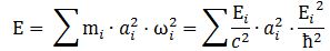 We can re-write this as:
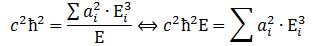 What is the meaning of this equation? We may look at it as some sort of physical normalization condition when building up the Fourier sum. Of course, we should relate this to the mathematical normalization condition for the wavefunction. Our intuition tells us that the probabilities must be related to the energy densities, but how exactly? We will come back to this question in a moment. Let us first think some more about the enigma: what is mass?
Before we do so, let us quickly calculate the value of c2ħ2: it is about 1´10–51 N2∙m4. Let us also do a dimensional analysis: the physical dimensions of the E = m·a2·ω2 equation make sense if we express m in kg, a in m, and ω in rad/s. We then get: [E] = kg∙m2/s2 = (N∙s2/m)∙m2/s2 = N∙m = J. The dimensions of the left- and right-hand side of the physical normalization condition is N3∙m5.
III. What is mass?
We came up, playfully, with a meaningful interpretation for energy: it is a two-dimensional oscillation of mass. But what is mass? A new aether theory is, of course, not an option, but then what is it that is oscillating? To understand the physics behind equations, it is always good to do an analysis of the physical dimensions in the equation. Let us start with Einstein’s energy equation once again. If we want to look at mass, we should re-write it as m = E/c2:
[m] = [E/c2] = J/(m/s)2 = N·m∙s2/m2 = N·s2/m = kg
This is not very helpful. It only reminds us of Newton’s definition of a mass: mass is that what gets accelerated by a force. At this point, we may want to think of the physical significance of the absolute nature of the speed of light. Einstein’s E = mc2 equation implies we can write the ratio between the energy and the mass of any particle is always the same, so we can write, for example: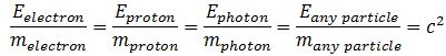 This reminds us of the ω2= C–1/L or ω2 = k/m of harmonic oscillators once again.[13] The key difference is that the ω2= C–1/L and ω2 = k/m formulas introduce two or more degrees of freedom.[14] In contrast, c2= E/m for any particle, always. However, that is exactly the point: we can modulate the resistance, inductance and capacitance of electric circuits, and the stiffness of springs and the masses we put on them, but we live in one physical space only: our spacetime. Hence, the speed of light c emerges here as the defining property of spacetime – the resonant frequency, so to speak. We have no further degrees of freedom here.
The Planck-Einstein relation (for photons) and the de Broglie equation (for matter-particles) have an interesting feature: both imply that the energy of the oscillation is proportional to the frequency, with Planck’s constant as the constant of proportionality. Now, for one-dimensional oscillations – think of a guitar string, for example – we know the energy will be proportional to the square of the frequency. It is a remarkable observation: the two-dimensional matter-wave, or the electromagnetic wave, gives us two waves for the price of one, so to speak, each carrying half of the total energy of the oscillation but, as a result, we get a proportionality between E and f instead of between E and f2.
However, such reflections do not answer the fundamental question we started out with: what is mass? At this point, it is hard to go beyond the circular definition that is implied by Einstein’s formula: energy is a two-dimensional oscillation of mass, and mass packs energy, and c emerges us as the property of spacetime that defines how exactly.
When everything is said and done, this does not go beyond stating that mass is some scalar field. Now, a scalar field is, quite simply, some real number that we associate with a position in spacetime. The Higgs field is a scalar field but, of course, the theory behind it goes much beyond stating that we should think of mass as some scalar field. The fundamental question is: why and how does energy, or matter, condense into elementary particles? That is what the Higgs mechanism is about but, as this paper is exploratory only, we cannot even start explaining the basics of it.
What we can do, however, is look at the wave equation again (Schrödinger’s equation), as we can now analyze it as an energy diffusion equation.
IV. Schrödinger’s equation as an energy diffusion equation
The interpretation of Schrödinger’s equation as a diffusion equation is straightforward. Feynman (Lectures, III-16-1) briefly summarizes it as follows:
“We can think of Schrödinger’s equation as describing the diffusion of the probability amplitude from one point to the next. […] But the imaginary coefficient in front of the derivative makes the behavior completely different from the ordinary diffusion such as you would have for a gas spreading out along a thin tube. Ordinary diffusion gives rise to real exponential solutions, whereas the solutions of Schrödinger’s equation are complex waves.”[17]
Let us review the basic math. For a particle moving in free space – with no external force fields acting on it – there is no potential (U = 0) and, therefore, the Uψ term disappears. Therefore, Schrödinger’s equation reduces to:
∂ψ(x, t)/∂t = i·(1/2)·(ħ/meff)·∇2ψ(x, t)
The ubiquitous diffusion equation in physics is:
∂φ(x, t)/∂t = D·∇2φ(x, t)
The structural similarity is obvious. The key difference between both equations is that the wave equation gives us two equations for the price of one. Indeed, because ψ is a complex-valued function, with a real and an imaginary part, we get the following equations[18]:
- Re(∂ψ/∂t) = −(1/2)·(ħ/meff)·Im(∇2ψ)
- Im(∂ψ/∂t) = (1/2)·(ħ/meff)·Re(∇2ψ)
These equations make us think of the equations for an electromagnetic wave in free space (no stationary charges or currents):
- ∂B/∂t = –∇×E
- ∂E/∂t = c2∇×B
The above equations effectively describe a propagation mechanism in spacetime, as illustrated below.
Figure 4: Propagation mechanisms
The Laplacian operator (∇2), when operating on a scalar quantity, gives us a flux density, i.e. something expressed per square meter (1/m2). In this case, it is operating on ψ(x, t), so what is the dimension of our wavefunction ψ(x, t)? To answer that question, we should analyze the diffusion constant in Schrödinger’s equation, i.e. the (1/2)·(ħ/meff) factor:
- As a mathematical constant of proportionality, it will quantify the relationship between both derivatives (i.e. the time derivative and the Laplacian);
- As a physical constant, it will ensure the physical dimensions on both sides of the equation are compatible.
Now, the ħ/meff factor is expressed in (N·m·s)/(N· s2/m) = m2/s. Hence, it does ensure the dimensions on both sides of the equation are, effectively, the same: ∂ψ/∂t is a time derivative and, therefore, its dimension is s–1 while, as mentioned above, the dimension of ∇2ψ is m–2. However, this does not solve our basic question: what is the dimension of the real and imaginary part of our wavefunction?
At this point, mainstream physicists will say: it does not have a physical dimension, and there is no geometric interpretation of Schrödinger’s equation. One may argue, effectively, that its argument, (p∙x – E∙t)/ħ, is just a number and, therefore, that the real and imaginary part of ψ is also just some number.
To this, we may object that ħ may be looked as a mathematical scaling constant only. If we do that, then the argument of ψ will, effectively, be expressed in action units, i.e. in N·m·s. It then does make sense to also associate a physical dimension with the real and imaginary part of ψ. What could it be?
We may have a closer look at Maxwell’s equations for inspiration here. The electric field vector is expressed in newton (the unit of force) per unit of charge (coulomb). Now, there is something interesting here. The physical dimension of the magnetic field is N/C divided by m/s.[19] We may write B as the following vector cross-product: B = (1/c)∙ex×E, with ex the unit vector pointing in the x-direction (i.e. the direction of propagation of the wave). Hence, we may associate the (1/c)∙ex× operator, which amounts to a rotation by 90 degrees, with the s/m dimension. Now, multiplication by i also amounts to a rotation by 90° degrees. Hence, we may boldly write: B = (1/c)∙ex×E = (1/c)∙i∙E. This allows us to also geometrically interpret Schrödinger’s equation in the way we interpreted it above (see Figure 3).[20]
Still, we have not answered the question as to what the physical dimension of the real and imaginary part of our wavefunction should be. At this point, we may be inspired by the structural similarity between Newton’s and Coulomb’s force laws: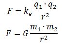 Hence, if the electric field vector E is expressed in force per unit charge (N/C), then we may want to think of associating the real part of our wavefunction with a force per unit mass (N/kg). We can, of course, do a substitution here, because the mass unit (1 kg) is equivalent to 1 N·s2/m. Hence, our N/kg dimension becomes:
N/kg = N/(N·s2/m)= m/s2
What is this: m/s2? Is that the dimension of the a·cosθ term in the a·e−iθ = a·cosθ − i·a·sinθ wavefunction?
My answer is: why not? Think of it: m/s2 is the physical dimension of acceleration: the increase or decrease in velocity (m/s) per second. It ensures the wavefunction for any particle – matter-particles or particles with zero rest mass (photons) – and the associated wave equation (which has to be the same for all, as the spacetime we live in is one) are mutually consistent.
In this regard, we should think of how we would model a gravitational wave. The physical dimension would surely be the same: force per mass unit. It all makes sense: wavefunctions may, perhaps, be interpreted as traveling distortions of spacetime, i.e. as tiny gravitational waves.
V. Energy densities and flows
Pursuing the geometric equivalence between the equations for an electromagnetic wave and Schrödinger’s equation, we can now, perhaps, see if there is an equivalent for the energy density. For an electromagnetic wave, we know that the energy density is given by the following formula: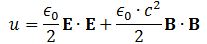 E and B are the electric and magnetic field vector respectively. The Poynting vector will give us the directional energy flux, i.e. the energy flow per unit area per unit time. We write:
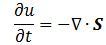 Needless to say, the ∇∙ operator is the divergence and, therefore, gives us the magnitude of a (vector) field’s source or sink at a given point. To be precise, the divergence gives us the volume density of the outward flux of a vector field from an infinitesimal volume around a given point. In this case, it gives us the volume density of the flux of S.
We can analyze the dimensions of the equation for the energy density as follows:
- E is measured in newton per coulomb, so [E∙E] = [E2] = N2/C2.
- B is measured in (N/C)/(m/s), so we get [B∙B] = [B2] = (N2/C2)·(s2/m2). However, the dimension of our c2 factor is (m2/s2) and so we’re also left with N2/C2.
- The ϵ0 is the electric constant, aka as the vacuum permittivity. As a physical constant, it should ensure the dimensions on both sides of the equation work out, and they do: [ε0] = C2/(N·m2) and, therefore, if we multiply that with N2/C2, we find that u is expressed in J/m3.[21]
Replacing the newton per coulomb unit (N/C) by the newton per kg unit (N/kg) in the formulas above should give us the equivalent of the energy density for the wavefunction. We just need to substitute ϵ0 for an equivalent constant. We may to give it a try. If the energy densities can be calculated – which are also mass densities, obviously – then the probabilities should be proportional to them.
Let us first see what we get for a photon, assuming the electromagnetic wave represents its wavefunction. Substituting B for (1/c)∙i∙E or for −(1/c)∙i∙E gives us the following result: Zero!? An unexpected result! Or not? We have no stationary charges and no currents: only an electromagnetic wave in free space. Hence, the local energy conservation principle needs to be respected at all points in space and in time. The geometry makes sense of the result: for an electromagnetic wave, the magnitudes of E and B reach their maximum, minimum and zero point simultaneously, as shown below.[22] This is because their phase is the same.
Figure 5: Electromagnetic wave: E and B
Should we expect a similar result for the energy densities that we would associate with the real and imaginary part of the matter-wave? For the matter-wave, we have a phase difference between a·cosθ and a·sinθ, which gives a different picture of the propagation of the wave (see Figure 3).[23] In fact, the geometry of the suggestion suggests some inherent spin, which is interesting. I will come back to this. Let us first guess those densities. Making abstraction of any scaling constants, we may write: We get what we hoped to get: the absolute square of our amplitude is, effectively, an energy density !
|ψ|2 = |a·e−i∙E·t/ħ|2 = a2 = u
This is very deep. A photon has no rest mass, so it borrows and returns energy from empty space as it travels through it. In contrast, a matter-wave carries energy and, therefore, has some (rest) mass. It is therefore associated with an energy density, and this energy density gives us the probabilities. Of course, we need to fine-tune the analysis to account for the fact that we have a wave packet rather than a single wave, but that should be feasible.
As mentioned, the phase difference between the real and imaginary part of our wavefunction (a cosine and a sine function) appear to give some spin to our particle. We do not have this particularity for a photon. Of course, photons are bosons, i.e. spin-zero particles, while elementary matter-particles are fermions with spin-1/2. Hence, our geometric interpretation of the wavefunction suggests that, after all, there may be some more intuitive explanation of the fundamental dichotomy between bosons and fermions, which puzzled even Feynman:
“Why is it that particles with half-integral spin are Fermi particles, whereas particles with integral spin are Bose particles? We apologize for the fact that we cannot give you an elementary explanation. An explanation has been worked out by Pauli from complicated arguments of quantum field theory and relativity. He has shown that the two must necessarily go together, but we have not been able to find a way of reproducing his arguments on an elementary level. It appears to be one of the few places in physics where there is a rule which can be stated very simply, but for which no one has found a simple and easy explanation. The explanation is deep down in relativistic quantum mechanics. This probably means that we do not have a complete understanding of the fundamental principle involved.” (Feynman, Lectures, III-4-1)
The physical interpretation of the wavefunction, as presented here, may provide some better understanding of ‘the fundamental principle involved’: the physical dimension of the oscillation is just very different. That is all: it is force per unit charge for photons, and force per unit mass for matter-particles. We will examine the question of spin somewhat more carefully in section VII. Let us first examine the matter-wave some more.
VI. Group and phase velocity of the matter-wave
The geometric representation of the matter-wave (see Figure 3) suggests a traveling wave and, yes, of course: the matter-wave effectively travels through space and time. But what is traveling, exactly? It is the pulse – or the signal – only: the phase velocity of the wave is just a mathematical concept and, even in our physical interpretation of the wavefunction, the same is true for the group velocity of our wave packet. The oscillation is two-dimensional, but perpendicular to the direction of travel of the wave. Hence, nothing actually moves with our particle.
Here, we should also reiterate that we did not answer the question as to what is oscillating up and down and/or sideways: we only associated a physical dimension with the components of the wavefunction – newton per kg (force per unit mass), to be precise. We were inspired to do so because of the physical dimension of the electric and magnetic field vectors (newton per coulomb, i.e. force per unit charge) we associate with electromagnetic waves which, for all practical purposes, we currently treat as the wavefunction for a photon. This made it possible to calculate the associated energy densities and a Poynting vector for energy dissipation. In addition, we showed that Schrödinger’s equation itself then becomes a diffusion equation for energy. However, let us now focus some more on the asymmetry which is introduced by the phase difference between the real and the imaginary part of the wavefunction. Look at the mathematical shape of the elementary wavefunction once again:
ψ = a·e−i[E·t − p∙x]/ħ = a·e−i[E·t − p∙x]/ħ = a·cos(p∙x/ħ − E∙t/ħ) + i·a·sin(p∙x/ħ − E∙t/ħ)
The minus sign in the argument of our sine and cosine function defines the direction of travel: an F(x−v∙t) wavefunction will always describe some wave that is traveling in the positive x-direction (with c the wave velocity), while an F(x+v∙t) wavefunction will travel in the negative x-direction. For a geometric interpretation of the wavefunction in three dimensions, we need to agree on how to define i or, what amounts to the same, a convention on how to define clockwise and counterclockwise directions: if we look at a clock from the back, then its hand will be moving counterclockwise. So we need to establish the equivalent of the right-hand rule. However, let us not worry about that now. Let us focus on the interpretation. To ease the analysis, we’ll assume we’re looking at a particle at rest. Hence, p = 0, and the wavefunction reduces to:
ψ = a·e−i∙E·t/ħ = a·cos(−E∙t/ħ) + i·a·sin(−E0∙t/ħ) = a·cos(E0∙t/ħ) − i·a·sin(E0∙t/ħ)
E0 is, of course, the rest mass of our particle and, now that we are here, we should probably wonder whose time t we are talking about: is it our time, or is the proper time of our particle? Well… In this situation, we are both at rest so it does not matter: t is, effectively, the proper time so perhaps we should write it as t0. It does not matter. You can see what we expect to see: E0/ħ pops up as the natural frequency of our matter-particle: (E0/ħ)∙t = ω∙t. Remembering the ω = 2π·f = 2π/T and T = 1/f formulas, we can associate a period and a frequency with this wave, using the ω = 2π·f = 2π/T. Noting that ħ = h/2π, we find the following:
T = 2π·(ħ/E0) = h/E0 ⇔ f = E0/h = m0c2/h
This is interesting, because we can look at the period as a natural unit of time for our particle. What about the wavelength? That is tricky because we need to distinguish between group and phase velocity here. The group velocity (vg) should be zero here, because we assume our particle does not move. In contrast, the phase velocity is given by vp = λ·f = (2π/k)·(ω/2π) = ω/k. In fact, we’ve got something funny here: the wavenumber k = p/ħ is zero, because we assume the particle is at rest, so p = 0. So we have a division by zero here, which is rather strange. What do we get assuming the particle is not at rest? We write:
vp = ω/k = (E/ħ)/(p/ħ) = E/p = E/(m·vg) = (m·c2)/(m·vg) = c2/vg
This is interesting: it establishes a reciprocal relation between the phase and the group velocity, with c as a simple scaling constant. Indeed, the graph below shows the shape of the function does not change with the value of c, and we may also re-write the relation above as:
vp/c = βp = c/vp = 1/βg = 1/(c/vp)
Figure 6: Reciprocal relation between phase and group velocity
We can also write the mentioned relationship as vp·vg = c2, which reminds us of the relationship between the electric and magnetic constant (1/ε0)·(1/μ0) = c2. This is interesting in light of the fact we can re-write this as (c·ε0)·(c·μ0) = 1, which shows electricity and magnetism are just two sides of the same coin, so to speak.[24]
Interesting, but how do we interpret the math? What about the implications of the zero value for wavenumber k = p/ħ. We would probably like to think it implies the elementary wavefunction should always be associated with some momentum, because the concept of zero momentum clearly leads to weird math: something times zero cannot be equal to c2! Such interpretation is also consistent with the Uncertainty Principle: if Δx·Δp ≥ ħ, then neither Δx nor Δp can be zero. In other words, the Uncertainty Principle tells us that the idea of a pointlike particle actually being at some specific point in time and in space does not make sense: it has to move. It tells us that our concept of dimensionless points in time and space are mathematical notions only. Actual particles – including photons – are always a bit spread out, so to speak, and – importantly – they have to move.
For a photon, this is self-evident. It has no rest mass, no rest energy, and, therefore, it is going to move at the speed of light itself. We write: p = m·c = m·c2/c = E/c. Using the relationship above, we get:
vp = ω/k = (E/ħ)/(p/ħ) = E/p = c ⇒ vg = c2/vp = c2/c = c
This is good: we started out with some reflections on the matter-wave, but here we get an interpretation of the electromagnetic wave as a wavefunction for the photon. But let us get back to our matter-wave. In regard to our interpretation of a particle having to move, we should remind ourselves, once again, of the fact that an actual particle is always localized in space and that it can, therefore, not be represented by the elementary wavefunction ψ = a·e−i[E·t − p∙x]/ħ or, for a particle at rest, the ψ = a·e−i∙E·t/ħ function. We must build a wave packet for that: a sum of wavefunctions, each with their own amplitude ai, and their own ωi = −Ei/ħ. Indeed, in section II, we showed that each of these wavefunctions will contribute some energy to the total energy of the wave packet and that, to calculate the contribution of each wave to the total, both ai as well as Ei matter. This may or may not resolve the apparent paradox. Let us look at the group velocity.
To calculate a meaningful group velocity, we must assume the vg = ∂ωi/∂ki = ∂(Ei/ħ)/∂(pi/ħ) = ∂(Ei)/∂(pi) exists. So we must have some dispersion relation. How do we calculate it? We need to calculate ωi as a function of ki here, or Ei as a function of pi. How do we do that? Well… There are a few ways to go about it but one interesting way of doing it is to re-write Schrödinger’s equation as we did, i.e. by distinguishing the real and imaginary parts of the ∂ψ/∂t =i·[ħ/(2m)]·∇2ψ wave equation and, hence, re-write it as the following pair of two equations:
- Re(∂ψ/∂t) = −[ħ/(2meff)]·Im(∇2ψ) ⇔ ω·cos(kx − ωt) = k2·[ħ/(2meff)]·cos(kx − ωt)
- Im(∂ψ/∂t) = [ħ/(2meff)]·Re(∇2ψ) ⇔ ω·sin(kx − ωt) = k2·[ħ/(2meff)]·sin(kx − ωt)
Both equations imply the following dispersion relation:
ω = ħ·k2/(2meff)
Of course, we need to think about the subscripts now: we have ωi, ki, but… What about meff or, dropping the subscript, m? Do we write it as mi? If so, what is it? Well… It is the equivalent mass of Ei obviously, and so we get it from the mass-energy equivalence relation: mi = Ei/c2. It is a fine point, but one most people forget about: they usually just write m. However, if there is uncertainty in the energy, then Einstein’s mass-energy relation tells us we must have some uncertainty in the (equivalent) mass too. Here, I should refer back to Section II: Ei varies around some average energy E and, therefore, the Uncertainty Principle kicks in.
VII. Explaining spin
The elementary wavefunction vector – i.e. the vector sum of the real and imaginary component – rotates around the x-axis, which gives us the direction of propagation of the wave (see Figure 3). Its magnitude remains constant. In contrast, the magnitude of the electromagnetic vector – defined as the vector sum of the electric and magnetic field vectors – oscillates between zero and some maximum (see Figure 5).
We already mentioned that the rotation of the wavefunction vector appears to give some spin to the particle. Of course, a circularly polarized wave would also appear to have spin (think of the E and B vectors rotating around the direction of propagation – as opposed to oscillating up and down or sideways only). In fact, a circularly polarized light does carry angular momentum, as the equivalent mass of its energy may be thought of as rotating as well. But so here we are looking at a matter-wave.
The basic idea is the following: if we look at ψ = a·e−i∙E·t/ħ as some real vector – as a two-dimensional oscillation of mass, to be precise – then we may associate its rotation around the direction of propagation with some torque. The illustration below reminds of the math here.
Figure 7: Torque and angular momentum vectors
A torque on some mass about a fixed axis gives it angular momentum, which we can write as the vector cross-product L = r×p or, perhaps easier for our purposes here as the product of an angular velocity (ω) and rotational inertia (I), aka as the moment of inertia or the angular mass. We write:
L = I·ω
Note we can write L and ω in boldface here because they are (axial) vectors. If we consider their magnitudes only, we write L = I·ω (no boldface). We can now do some calculations. Let us start with the angular velocity. In our previous posts, we showed that the period of the matter-wave is equal to T = 2π·(ħ/E0). Hence, the angular velocity must be equal to:
ω = 2π/[2π·(ħ/E0)] = E0/ħ
We also know the distance r, so that is the magnitude of r in the L = r×p vector cross-product: it is just a, so that is the magnitude of ψ = a·e−i∙E·t/ħ. Now, the momentum (p) is the product of a linear velocity (v) – in this case, the tangential velocity – and some mass (m): p = m·v. If we switch to scalar instead of vector quantities, then the (tangential) velocity is given by v = r·ω. So now we only need to think about what we should use for m or, if we want to work with the angular velocity (ω), the angular mass (I). Here we need to make some assumption about the mass (or energy) distribution. Now, it may or may not sense to assume the energy in the oscillation – and, therefore, the mass – is distributed uniformly. In that case, we may use the formula for the angular mass of a solid cylinder: I = m·r2/2. If we keep the analysis non-relativistic, then m = m0. Of course, the energy-mass equivalence tells us that m0 = E0/c2. Hence, this is what we get:
L = I·ω = (m0·r2/2)·(E0/ħ) = (1/2)·a2·(E0/c2)·(E0/ħ) = a2·E02/(2·ħ·c2)
Does it make sense? Maybe. Maybe not. Let us do a dimensional analysis: that won’t check our logic, but it makes sure we made no mistakes when mapping mathematical and physical spaces. We have m2·J2 = m2·N2·m2 in the numerator and N·m·s·m2/s2 in the denominator. Hence, the dimensions work out: we get N·m·s as the dimension for L, which is, effectively, the physical dimension of angular momentum. It is also the action dimension, of course, and that cannot be a coincidence. Also note that the E = mc2 equation allows us to re-write it as:
L = a2·E02/(2·ħ·c2)
Of course, in quantum mechanics, we associate spin with the magnetic moment of a charged particle, not with its mass as such. Is there way to link the formula above to the one we have for the quantum-mechanical angular momentum, which is also measured in N·m·s units, and which can only take on one of two possible values: J = +ħ/2 and −ħ/2? It looks like a long shot, right? How do we go from (1/2)·a2·m02/ħ to ± (1/2)∙ħ? Let us do a numerical example. The energy of an electron is typically 0.510 MeV » 8.1871×10⁻¹⁴ N∙m, and a… What value should we take for a?
We have an obvious trio of candidates here: the Bohr radius, the classical electron radius (aka the Thompon scattering length), and the Compton scattering radius.
Let us start with the Bohr radius, so that is about 0.×10−10 N∙m. We get L = a2·E02/(2·ħ·c2) = 9.9×10⁻³¹ N∙m∙s. Now that is about 1.88×10⁴ times ħ/2. That is a huge factor. The Bohr radius cannot be right: we are not looking at an electron in an orbital here. To show it does not make sense, we may want to double-check the analysis by doing the calculation in another way. We said each oscillation will always pack 6.626070040(81)×10−34 joule in energy. So our electron should pack about 1.24×10⁻²⁰ oscillations. The angular momentum (L) we get when using the Bohr radius for a and the value of 6.626×10⁻³⁴ joule for E0 and the Bohr radius is equal to 6.49×10−59 N∙m∙s. So that is the angular momentum per oscillation. When we multiply this with the number of oscillations (1.24×10⁻²⁰), we get about 8.01×10−51 N∙m∙s, so that is a totally different number.
The classical electron radius is about 2.818×10⁻¹⁵ m. We get an L that is equal to about 2.81×10−39 N∙m∙s, so now it is a tiny fraction of ħ/2! Hence, this leads us nowhere. Let us go for our last chance to get a meaningful result! Let us use the Compton scattering length, so that is about 2.42631×10⁻¹² m.
This gives us an L of 2.08×10⁻³³ N∙m∙s, which is only 20 times ħ. This is not so bad, but it is good enough? Let us calculate it the other way around: what value should we take for a so as to ensure L = a2·E02/(2·ħ·c2) = ħ/2? Let us write it out:
In fact, this is the formula for the so-called reduced Compton wavelength. This is perfect. We found what we wanted to find. Substituting this value for a (you can calculate it: it is about 3.8616×10⁻³³ m), we get what we should find:
This is a rather spectacular result, and one that would – a priori – support the interpretation of the wavefunction that is being suggested in this paper.
VIII. The boson-fermion dichotomy
Let us do some more thinking on the boson-fermion dichotomy. Again, we should remind ourselves that an actual particle is localized in space and that it can, therefore, not be represented by the elementary wavefunction ψ = a·e−i[E·t − p∙x]/ħ or, for a particle at rest, the ψ = a·e−i∙E·t/ħ function. We must build a wave packet for that: a sum of wavefunctions, each with their own amplitude ai, and their own ωi = −Ei/ħ. Each of these wavefunctions will contribute some energy to the total energy of the wave packet. Now, we can have another wild but logical theory about this.
Think of the apparent right-handedness of the elementary wavefunction: surely, Nature can’t be bothered about our convention of measuring phase angles clockwise or counterclockwise. Also, the angular momentum can be positive or negative: J = +ħ/2 or −ħ/2. Hence, we would probably like to think that an actual particle – think of an electron, or whatever other particle you’d think of – may consist of right-handed as well as left-handed elementary waves. To be precise, we may think they either consist of (elementary) right-handed waves or, else, of (elementary) left-handed waves. An elementary right-handed wave would be written as:
ψ(θi) = ai·(cosθi + i·sinθi)
In contrast, an elementary left-handed wave would be written as:
ψ(θi) = ai·(cosθi − i·sinθi)
How does that work out with the E0·t argument of our wavefunction? Position is position, and direction is direction, but time? Time has only one direction, but Nature surely does not care how we count time: counting like 1, 2, 3, etcetera or like −1, −2, −3, etcetera is just the same. If we count like 1, 2, 3, etcetera, then we write our wavefunction like:
ψ = a·cos(E0∙t/ħ) − i·a·sin(E0∙t/ħ)
If we count time like −1, −2, −3, etcetera then we write it as:
ψ = a·cos(−E0∙t/ħ) − i·a·sin(−E0∙t/ħ)= a·cos(E0∙t/ħ) + i·a·sin(E0∙t/ħ)
Hence, it is just like the left- or right-handed circular polarization of an electromagnetic wave: we can have both for the matter-wave too! This, then, should explain why we can have either positive or negative quantum-mechanical spin (+ħ/2 or −ħ/2). It is the usual thing: we have two mathematical possibilities here, and so we must have two physical situations that correspond to it.
It is only natural. If we have left- and right-handed photons – or, generalizing, left- and right-handed bosons – then we should also have left- and right-handed fermions (electrons, protons, etcetera). Back to the dichotomy. The textbook analysis of the dichotomy between bosons and fermions may be epitomized by Richard Feynman’s Lecture on it (Feynman, III-4), which is confusing and – I would dare to say – even inconsistent: how are photons or electrons supposed to know that they need to interfere with a positive or a negative sign? They are not supposed to know anything: knowledge is part of our interpretation of whatever it is that is going on there.
Hence, it is probably best to keep it simple, and think of the dichotomy in terms of the different physical dimensions of the oscillation: newton per kg versus newton per coulomb. And then, of course, we should also note that matter-particles have a rest mass and, therefore, actually carry charge. Photons do not. But both are two-dimensional oscillations, and the point is: the so-called vacuum – and the rest mass of our particle (which is zero for the photon and non-zero for everything else) – give us the natural frequency for both oscillations, which is beautifully summed up in that remarkable equation for the group and phase velocity of the wavefunction, which applies to photons as well as matter-particles:
(vphase·c)·(vgroup·c) = 1 ⇔ vp·vg = c2
The final question then is: why are photons spin-zero particles? Well… We should first remind ourselves of the fact that they do have spin when circularly polarized.[25] Here we may think of the rotation of the equivalent mass of their energy. However, if they are linearly polarized, then there is no spin. Even for circularly polarized waves, the spin angular momentum of photons is a weird concept. If photons have no (rest) mass, then they cannot carry any charge. They should, therefore, not have any magnetic moment. Indeed, what I wrote above shows an explanation of quantum-mechanical spin requires both mass as well as charge.[26]
IX. Concluding remarks
There are, of course, other ways to look at the matter – literally. For example, we can imagine two-dimensional oscillations as circular rather than linear oscillations. Think of a tiny ball, whose center of mass stays where it is, as depicted below. Any rotation – around any axis – will be some combination of a rotation around the two other axes. Hence, we may want to think of a two-dimensional oscillation as an oscillation of a polar and azimuthal angle.
Figure 8: Two-dimensional circular movement
The point of this paper is not to make any definite statements. That would be foolish. Its objective is just to challenge the simplistic mainstream viewpoint on the reality of the wavefunction. Stating that it is a mathematical construct only without physical significance amounts to saying it has no meaning at all. That is, clearly, a non-sustainable proposition.
The interpretation that is offered here looks at amplitude waves as traveling fields. Their physical dimension may be expressed in force per mass unit, as opposed to electromagnetic waves, whose amplitudes are expressed in force per (electric) charge unit. Also, the amplitudes of matter-waves incorporate a phase factor, but this may actually explain the rather enigmatic dichotomy between fermions and bosons and is, therefore, an added bonus.
The interpretation that is offered here has some advantages over other explanations, as it explains the how of diffraction and interference. However, while it offers a great explanation of the wave nature of matter, it does not explain its particle nature: while we think of the energy as being spread out, we will still observe electrons and photons as pointlike particles once they hit the detector. Why is it that a detector can sort of ‘hook’ the whole blob of energy, so to speak?
The interpretation of the wavefunction that is offered here does not explain this. Hence, the complementarity principle of the Copenhagen interpretation of the wavefunction surely remains relevant.
Appendix 1: The de Broglie relations and energy
The 1/2 factor in Schrödinger’s equation is related to the concept of the effective mass (meff). It is easy to make the wrong calculations. For example, when playing with the famous de Broglie relations – aka as the matter-wave equations – one may be tempted to derive the following energy concept:
- E = h·f and p = h/λ. Therefore, f = E/h and λ = p/h.
- v = f·λ = (E/h)∙(p/h) = E/p
- p = m·v. Therefore, E = v·p = m·v2
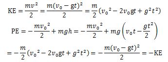
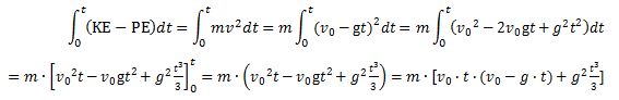
E = m·v2? This resembles the E = mc2 equation and, therefore, one may be enthused by the discovery, especially because the m·v2 also pops up when working with the Least Action Principle in classical mechanics, which states that the path that is followed by a particle will minimize the following integral: Now, we can choose any reference point for the potential energy but, to reflect the energy conservation law, we can select a reference point that ensures the sum of the kinetic and the potential energy is zero throughout the time interval. If the force field is uniform, then the integrand will, effectively, be equal to KE − PE = m·v2.[27]
However, that is classical mechanics and, therefore, not so relevant in the context of the de Broglie equations, and the apparent paradox should be solved by distinguishing between the group and the phase velocity of the matter wave.
Appendix 2: The concept of the effective mass
The effective mass – as used in Schrödinger’s equation – is a rather enigmatic concept. To make sure we are making the right analysis here, I should start by noting you will usually see Schrödinger’s equation written as: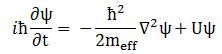 This formulation includes a term with the potential energy (U). In free space (no potential), this term disappears, and the equation can be re-written as:
∂ψ(x, t)/∂t = i·(1/2)·(ħ/meff)·∇2ψ(x, t)
We just moved the i·ħ coefficient to the other side, noting that 1/i = –i. Now, in one-dimensional space, and assuming ψ is just the elementary wavefunction (so we substitute a·e−i∙[E·t − p∙x]/ħ for ψ), this implies the following:
−a·i·(E/ħ)·e−i∙[E·t − p∙x]/ħ = −i·(ħ/2meff)·a·(p2/ħ2)· e−i∙[E·t − p∙x]/ħ
⇔ E = p2/(2meff) ⇔ meff = m∙(v/c)2/2 = m∙β2/2
It is an ugly formula: it resembles the kinetic energy formula (K.E. = m∙v2/2) but it is, in fact, something completely different. The β2/2 factor ensures the effective mass is always a fraction of the mass itself. To get rid of the ugly 1/2 factor, we may re-define meff as two times the old meff (hence, meffNEW = 2∙meffOLD), as a result of which the formula will look somewhat better:
meff = m∙(v/c)2 = m∙β2
We know β varies between 0 and 1 and, therefore, meff will vary between 0 and m. Feynman drops the subscript, and just writes meff as m in his textbook (see Feynman, III-19). On the other hand, the electron mass as used is also the electron mass that is used to calculate the size of an atom (see Feynman, III-2-4). As such, the two mass concepts are, effectively, mutually compatible. It is confusing because the same mass is often defined as the mass of a stationary electron (see, for example, the article on it in the online Wikipedia encyclopedia[28]).
In the context of the derivation of the electron orbitals, we do have the potential energy term – which is the equivalent of a source term in a diffusion equation – and that may explain why the above-mentioned meff = m∙(v/c)2 = m∙β2 formula does not apply.
References
This paper discusses general principles in physics only. Hence, references can be limited to references to physics textbooks only. For ease of reading, any reference to additional material has been limited to a more popular undergrad textbook that can be consulted online: Feynman’s Lectures on Physics (http://www.feynmanlectures.caltech.edu). References are per volume, per chapter and per section. For example, Feynman III-19-3 refers to Volume III, Chapter 19, Section 3.
Notes
[1] Of course, an actual particle is localized in space and can, therefore, not be represented by the elementary wavefunction ψ = a·e−i∙θ = a·e−i[E·t − p∙x]/ħ = a·(cosθ – i·a·sinθ). We must build a wave packet for that: a sum of wavefunctions, each with its own amplitude ak and its own argument θk = (Ek∙t – pk∙x)/ħ. This is dealt with in this paper as part of the discussion on the mathematical and physical interpretation of the normalization condition.
[2] The N/kg dimension immediately, and naturally, reduces to the dimension of acceleration (m/s2), thereby facilitating a direct interpretation in terms of Newton’s force law.
[3] In physics, a two-spring metaphor is more common. Hence, the pistons in the author’s perpetuum mobile may be replaced by springs.
[4] The author re-derives the equation for the Compton scattering radius in section VII of the paper.
[5] The magnetic force can be analyzed as a relativistic effect (see Feynman II-13-6). The dichotomy between the electric force as a polar vector and the magnetic force as an axial vector disappears in the relativistic four-vector representation of electromagnetism.
[6] For example, when using Schrödinger’s equation in a central field (think of the electron around a proton), the use of polar coordinates is recommended, as it ensures the symmetry of the Hamiltonian under all rotations (see Feynman III-19-3)
[7] This sentiment is usually summed up in the apocryphal quote: “God does not play dice.”The actual quote comes out of one of Einstein’s private letters to Cornelius Lanczos, another scientist who had also emigrated to the US. The full quote is as follows: “You are the only person I know who has the same attitude towards physics as I have: belief in the comprehension of reality through something basically simple and unified… It seems hard to sneak a look at God’s cards. But that He plays dice and uses ‘telepathic’ methods… is something that I cannot believe for a single moment.” (Helen Dukas and Banesh Hoffman, Albert Einstein, the Human Side: New Glimpses from His Archives, 1979)
[8] Of course, both are different velocities: ω is an angular velocity, while v is a linear velocity: ω is measured in radians per second, while v is measured in meter per second. However, the definition of a radian implies radians are measured in distance units. Hence, the physical dimensions are, effectively, the same. As for the formula for the total energy of an oscillator, we should actually write: E = m·a2∙ω2/2. The additional factor (a) is the (maximum) amplitude of the oscillator.
[9] We also have a 1/2 factor in the E = mv2/2 formula. Two remarks may be made here. First, it may be noted this is a non-relativistic formula and, more importantly, incorporates kinetic energy only. Using the Lorentz factor (γ), we can write the relativistically correct formula for the kinetic energy as K.E. = E − E0 = mvc2 − m0c2 = m0γc2 − m0c2 = m0c2(γ − 1). As for the exclusion of the potential energy, we may note that we may choose our reference point for the potential energy such that the kinetic and potential energy mirror each other. The energy concept that then emerges is the one that is used in the context of the Principle of Least Action: it equals E = mv2. Appendix 1 provides some notes on that.
[10] Instead of two cylinders with pistons, one may also think of connecting two springs with a crankshaft.
[11] It is interesting to note that we may look at the energy in the rotating flywheel as potential energy because it is energy that is associated with motion, albeit circular motion. In physics, one may associate a rotating object with kinetic energy using the rotational equivalent of mass and linear velocity, i.e. rotational inertia (I) and angular velocity ω. The kinetic energy of a rotating object is then given by K.E. = (1/2)·I·ω2.
[12] Because of the sideways motion of the connecting rods, the sinusoidal function will describe the linear motion only approximately, but you can easily imagine the idealized limit situation.
[13] The ω2= 1/LC formula gives us the natural or resonant frequency for a electric circuit consisting of a resistor (R), an inductor (L), and a capacitor (C). Writing the formula as ω2= C–1/L introduces the concept of elastance, which is the equivalent of the mechanical stiffness (k) of a spring.
[14] The resistance in an electric circuit introduces a damping factor. When analyzing a mechanical spring, one may also want to introduce a drag coefficient. Both are usually defined as a fraction of the inertia, which is the mass for a spring and the inductance for an electric circuit. Hence, we would write the resistance for a spring as γm and as R = γL respectively.
[15] Photons are emitted by atomic oscillators: atoms going from one state (energy level) to another. Feynman (Lectures, I-33-3) shows us how to calculate the Q of these atomic oscillators: it is of the order of 108, which means the wave train will last about 10–8 seconds (to be precise, that is the time it takes for the radiation to die out by a factor 1/e). For example, for sodium light, the radiation will last about 3.2×10⁻⁸ seconds (this is the so-called decay time τ). Now, because the frequency of sodium light is some 500 THz (500×1012 oscillations per second), this makes for some 16 million oscillations. There is an interesting paradox here: the speed of light tells us that such wave train will have a length of about 9.6 m! How is that to be reconciled with the pointlike nature of a photon? The paradox can only be explained by relativistic length contraction: in an analysis like this, one need to distinguish the reference frame of the photon – riding along the wave as it is being emitted, so to speak – and our stationary reference frame, which is that of the emitting atom.
[16] This is a general result and is reflected in the K.E. = T = (1/2)·m·ω2·a2·sin2(ω·t + Δ) and the P.E. = U = k·x2/2 = (1/2)· m·ω2·a2·cos2(ω·t + Δ) formulas for the linear oscillator.
[17] Feynman further formalizes this in his Lecture on Superconductivity (Feynman, III-21-2), in which he refers to Schrödinger’s equation as the “equation for continuity of probabilities”. The analysis is centered on the local conservation of energy, which confirms the interpretation of Schrödinger’s equation as an energy diffusion equation.
[18] The meff is the effective mass of the particle, which depends on the medium. For example, an electron traveling in a solid (a transistor, for example) will have a different effective mass than in an atom. In free space, we can drop the subscript and just write meff = m. Appendix 2 provides some additional notes on the concept. As for the equations, they are easily derived from noting that two complex numbers a + i∙b and c + i∙d are equal if, and only if, their real and imaginary parts are the same. Now, the ∂ψ/∂t = i∙(ħ/meff)∙∇2ψ equation amounts to writing something like this: a + i∙b = i∙(c + i∙d). Now, remembering that i2 = −1, you can easily figure out that i∙(c + i∙d) = i∙c + i2∙d = − d + i∙c.
[19] The dimension of B is usually written as N/(m∙A), using the SI unit for current, i.e. the ampere (A). However, 1 C = 1 A∙s and, hence, 1 N/(m∙A) = 1 (N/C)/(m/s).
[20] Of course, multiplication with i amounts to a counterclockwise rotation. Hence, multiplication by –i also amounts to a rotation by 90 degrees, but clockwise. Now, to uniquely identify the clockwise and counterclockwise directions, we need to establish the equivalent of the right-hand rule for a proper geometric interpretation of Schrödinger’s equation in three-dimensional space: if we look at a clock from the back, then its hand will be moving counterclockwise. When writing B = (1/c)∙i∙E, we assume we are looking in the negative x-direction. If we are looking in the positive x-direction, we should write: B = -(1/c)∙i∙E. Of course, Nature does not care about our conventions. Hence, both should give the same results in calculations. We will show in a moment they do.
[21] In fact, when multiplying C2/(N·m2) with N2/C2, we get N/m2, but we can multiply this with 1 = m/m to get the desired result. It is significant that an energy density (joule per unit volume) can also be measured in newton (force per unit area.
[22] The illustration shows a linearly polarized wave, but the obtained result is general.
[23] The sine and cosine are essentially the same functions, except for the difference in the phase: sinθ = cos(θ−π /2).
[24] I must thank a physics blogger for re-writing the 1/(ε0·μ0) = c2 equation like this. See: http://reciprocal.systems/phpBB3/viewtopic.php?t=236 (retrieved on 29 September 2017).
[25] A circularly polarized electromagnetic wave may be analyzed as consisting of two perpendicular electromagnetic plane waves of equal amplitude and 90° difference in phase.
[26] Of course, the reader will now wonder: what about neutrons? How to explain neutron spin? Neutrons are neutral. That is correct, but neutrons are not elementary: they consist of (charged) quarks. Hence, neutron spin can (or should) be explained by the spin of the underlying quarks.
[27] We detailed the mathematical framework and detailed calculations in the following online article: https://readingfeynman.org/2017/09/15/the-principle-of-least-action-re-visited.
[28] https://en.wikipedia.org/wiki/Electron_rest_mass (retrieved on 29 September 2017).

 Now, all oscillations of the elementary wavefunction have the same amplitude: a. [Terminology is a bit confusing here because we use the term amplitude to refer to two very different things here: we may say a is the amplitude of the (probability) amplitude ψ. So how many oscillations do we have? What is the size of our box? Let us assume our particle is an electron, and we will reduce its motion to a one-dimensional motion only: we’re thinking of it as traveling along the x-axis. We can then use the y- and z-axes as mathematical axes only: they will show us how the magnitude and direction of the real and imaginary component of ψ. The animation below (for which I have to credit Wikipedia) shows how it looks like.
 Of course, we can have right- as well as left-handed particle waves because, while time physically goes by in one direction only (we can’t reverse time), we can count it in two directions: 1, 2, 3, etcetera or −1, −2, −3, etcetera. In the latter case, think of
 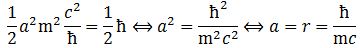 This is the formula for the radius of an electron. To be precise, it is the Compton scattering radius, so that’s the effective radius of an electron as determined by scattering experiments. You can calculate it: it is about 3.8616×10⁻¹³ m, so that’s the picometer scale, as we would expect.

 We find that m would have to be equal to m ≈ 1.11×10−36 kg. That’s tiny. In fact, it’s equivalent to an energy of about equivalent to 0.623 eV (which you’ll see written as 623 milli-eV. This corresponds to light with a wavelength of about 2 micro-meter (μm), so that’s in the infrared spectrum. It’s a funny formula: we find, basically, that the l/a ratio is proportional to m4. Hmm… What should we think of this? If you have any ideas, let me know !


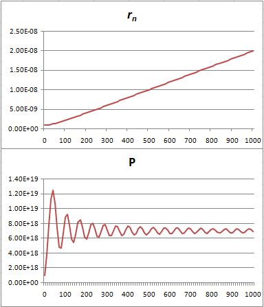
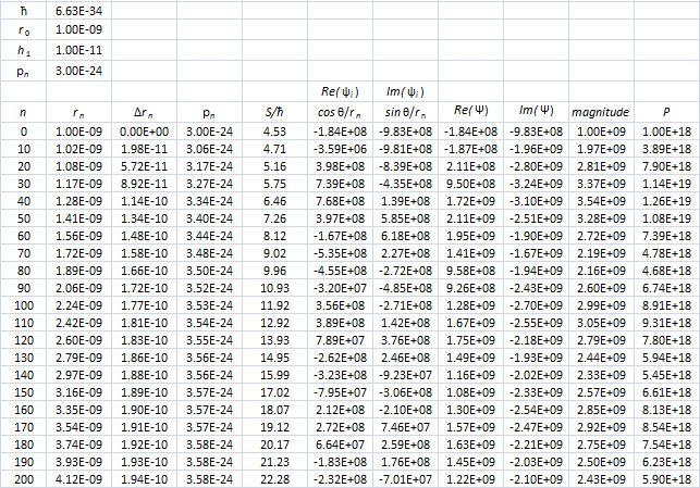
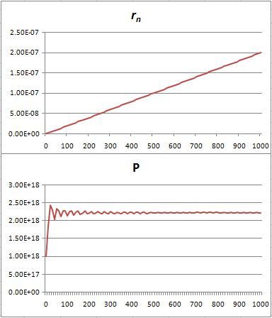
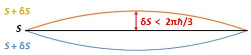
 Hence, if S0 is the action for r0, then S1 = S0 + ħ and S2 = S0 + 2·ħ are still good, but S3 = S0 + 3·ħ is not good. Why? Because the difference in the phase angles is Δθ = S1/ħ − S0/ħ = (S0 + ħ)/ħ − S0/ħ = 1 and Δθ = S2/ħ − S0/ħ = (S0 + 2·ħ)/ħ − S0/ħ = 2 respectively, so that’s 57.3° and 114.6° respectively and that’s, effectively, less than 120°. In contrast, for the next path, we find that Δθ = S3/ħ − S0/ħ = (S0 + 3·ħ)/ħ − S0/ħ = 3, so that’s 171.9°. So that amplitude gives us a negative contribution.
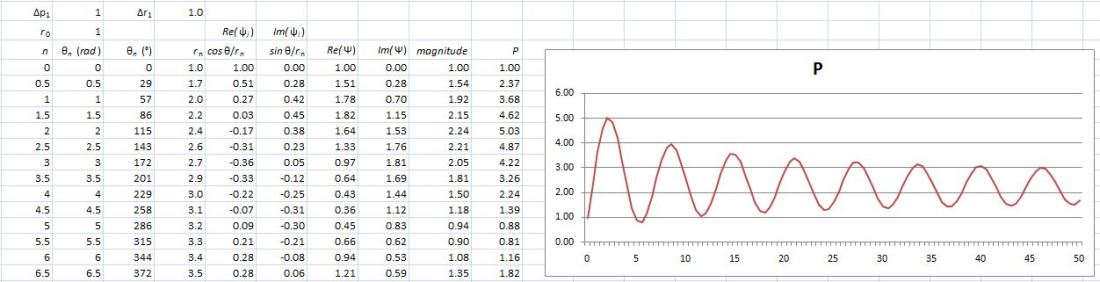 Well… We get a weird result. It reminds me of

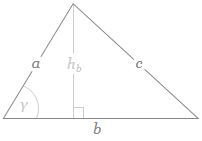 If b is the straight-line path (r0), then ac could be one of the crooked paths (rn). To simplify, we’ll assume isosceles triangles, so a equals c and, hence, rn = 2·a = 2·c. We will also assume the successive paths are separated by the same vertical distance (h = h1) right in the middle, so hb = hn = n·h1. It is then easy to show the following:

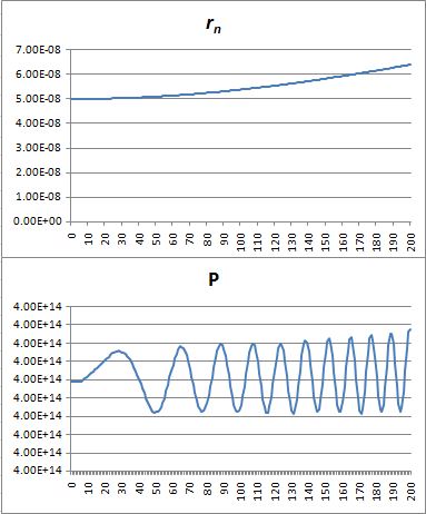 That’s because we increase the weight of the paths that are further removed from the center. So… Well… We shouldn’t be doing that, I guess. 🙂 I’ll you look for the right formula, OK? Let me know when you found it. 🙂


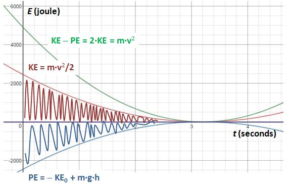
 Note the integrand: KE − PE = m·v2. Strange, isn’t it? It’s like E = m·c2, right? We get a weird cubic function, which I plotted below (

 Our simplified approach (the assumption of light traveling at the speed of light) reduces our least action principle to a least time principle: the arrows associated with the path of least time and the paths immediately left and right of it that make the biggest contribution to the final arrow. Why? Think of the stopwatch metaphor: these stopwatches arrive around the same time and, hence, their hands point more or less in the same direction. It doesn’t matter what direction – as long as it’s more or less the same.

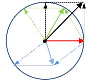 We need to note a few things here. First, unlike what you might think, the amplitudes of the higher and lower path in the drawing do not cancel. On the contrary, the action S is the same, so their magnitudes just add up. Second, if this logic is correct, we will have alternating zones with paths that interfere positively and negatively, as shown below.

 We know this elementary wavefunction cannot represent a real-life particle. Indeed, the a·e−i·θ function implies the probability of finding the particle – an electron, a photon, or whatever – would be equal to P(x, t) = |ψ(x, t)|2 = |a·e−(i/ħ)·(E·t−p·x)|2 = |a|2·|e−(i/ħ)·(E·t−p·x)|2 = |a|2·12= a2 everywhere. Hence, the particle would be everywhere – and, therefore, nowhere really. We need to localize the wave – or build a wave packet. We can do so by introducing uncertainty: we then add a potentially infinite number of these elementary wavefunctions with slightly different values for E and p, and various amplitudes a. Each of these amplitudes will then reflect the contribution to the composite wave, which – in three-dimensional space – we can write as:
 Hence, if we don’t change the direction of the y– and z-axes – so we keep defining the z-axis as the axis pointing upwards, and the y-axis as the axis pointing towards us – then the positive direction of the x-axis would actually be the direction from right to left, and we should say that the elementary wavefunction in the animation above seems to propagate in the negative x-direction. [Note that this left- or right-hand rule is quite astonishing: simply swapping the direction of one axis of a left-handed frame makes it right-handed, and vice versa.]

 The next illustration – of how water waves actually propagate – is, perhaps, more relevant. Just think of a two-dimensional equivalent – and of the two oscillations as being transverse waves, as opposed to longitudinal. See how string theory starts making sense? 🙂
 The most fundamental question remains the same: what is it, exactly, that is oscillating here? What is the field? It’s always some force on some charge – but what charge, exactly? Mass? What is it? Well… I don’t have the answer to that. It’s the same as asking: what is electric charge, really? So the question is: what’s the reality of mass, of electric charge, or whatever other charge that causes a force to act on it?
 Now that we’re talking mass, note a neutral pion (π0) may either be a uū or a dđ combination, and that the mass of a u-quark and a d-quark is only 2.4 and 4.8 MeV – so the binding energy of the constituent parts of this π0 particle is enormous: it accounts for most of its mass.

 The −g
 Aitchison and Hey call a, therefore, a range parameter: it effectively defines the range in which the n-p potential has a significant value: outside of the range, its value is, for all practical purposes, (close to) zero. Experimentally, this range was established as being more or less equal to r ≤ 2 fm. Needless to say, while this range factor may do its job, it’s obvious Yukawa’s formula for the n-p potential comes across as being somewhat random: what’s the theory behind? There’s none, really. It makes one think of
  What the heck? Relax. To derive this equation, we’d need to take a pretty complicated détour, which we won’t do. [See Appendix G of
  As said, you can look up the nitty-gritty in
  What? Yes. It’s a big thing to swallow, and it doesn’t help most physicists refer to U as a force field. A force and the potential that results from it are two different things. To put it simply: the force on an object is not the same as the work you need to move it from here to there. Force and potential are related but different concepts. Having said that, it sort of make sense now, doesn’t it? If potential is energy, and if it behaves like some wave, then we must be able to associate it with a de Broglie-type particle. This U-quantum, as it is referred to, comes in two varieties, which are associated with the ongoing absorption-emission process that is supposed to take place inside of the nucleus (depicted below):
 Now, it doesn’t take too many gimmicks to compare this against the relativistically correct energy-momentum relation:
 Combining both gives us the associated (rest) mass of the U-quantum:
 For a ≈ 2 fm, m
 An alternative – and simpler – way of representing this exchange of a virtual particle (a neutral pion in this case) is obtained by drawing a so-called Feynman diagram:
 OK. That’s it for today. More tomorrow. 🙂
 When analyzing this animation – look at the movement of the green, red and blue dots respectively – one cannot miss the equivalence between this oscillation and the movement of a mass on a spring – as depicted below.
 The e−i·(E/ħ)·t function just gives us two springs for the price of one. 🙂 Now, you may want to imagine some kind of elastic medium –


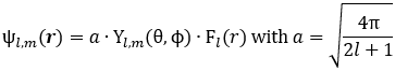 Note
Note 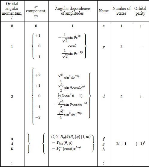 The Plm(cosθ) functions are the so-called
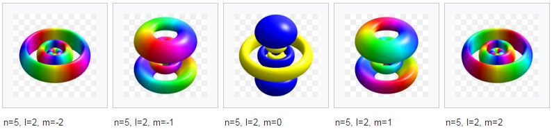
 So… To make a long story short, we can substitute the cosθ argument in the Plm(cosθ) function for sinα = sin(π/2 − θ). Now, if the xy-plane is a symmetry plane, then we must find the same value for Plm(sinα) and Plm[sin(−α)]. Now, that’s not obvious, because sin(−α) = −sinα ≠ sinα. However, because the argument in that Plm(x) function is being squared before any other operation (like subtracting 1 and exponentiating the result), it is OK: [−sinα]2 = [sinα]2 = sin2α. […] OK, I am sure the geeks amongst my readers will be able to explain this more rigorously. In fact, I hope they’ll have a look at it, because there’s also that dl+m/dxl+m operator, and so you should check what happens with the minus sign there. 🙂
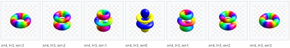
 The Yl,m(θ, φ) and Fn,l(ρ) functions here are functions of the (polar) coordinates ρ, θ, φ only. So that’s the position only (these coordinates are polar or spherical coordinates, so ρ is the radial distance, θ is the polar angle, and φ is the azimuthal angle). There’s no idea whatsoever of any momentum in one or the other spatial direction here. I find that rather remarkable. Let’s see how it all works with a simple example.
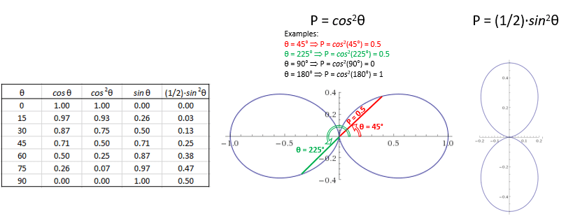 These polar graphs are not so easy to interpret, so let me say a few words about them. The points that are plotted combine (a) some radial distance from the center – which I wrote as P because this distance is, effectively, a probability – with (b) the polar angle θ (so that’s one of the three coordinates). To be precise, the plot gives us, for a given ρ, all of the (θ, P) combinations. It works as follows. To calculate the probability for some ρ and θ (note that φ can be any angle), we must take the absolute square of that ψn,l,m, = Yl,m(θ, φ)·Fn,l(ρ) product. Hence, we must calculate |Yl,m(θ, φ)·Fn,l(ρ)|2 = |Fn,l(ρ)|2·cos2θ for m = 0, and (1/2)·|Fn,l(ρ)|2·sin2θ for m = ±1. Hence, the value of ρ determines the value of Fn,l(ρ), and that Fn,l(ρ) value then determines the shape of the polar graph. The three graphs below – P = cos2θ, P = (1/2)·cos2θ and P = (1/4)·cos2θ – illustrate the idea.
 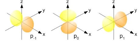 Three lobes. Well… Frankly, I am not quite sure here, but the equations speak for themselves: the probabilities only depend on ρ and θ. Hence, the azimuthal angle φ can be anything. So you just need to rotate those P = (1/2)·sin2θ and P = cos2θ curves about the the z-axis. In case you wonder how to do that, the illustration below may inspire you.
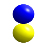


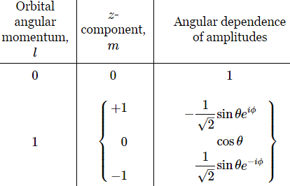
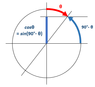 In contrast, the ei·φ and/or e−i·φ factor work very differently. These just give us a phase shift, as illustrated below. A re-set of our zero point for measuring time, so to speak, and the ei·φ and/or e−i·φ factor effectively disappears when we’re calculating probabilities, which is consistent with the fact that this angle clearly doesn’t influence the magnitude of the amplitude fluctuations.
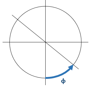 So… Well… That’s it, really. I hope you enjoyed this ! 🙂
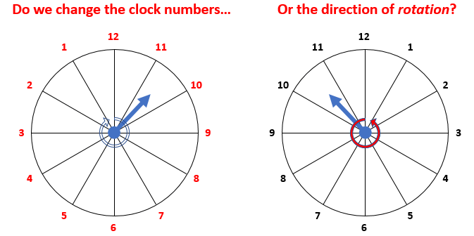 Now, imagine you’re the dictator who decided to change our time measuring convention. How would you go about it? Would you change the numbers on the clock or the direction of rotation? Personally, I’d be in favor of changing the direction of rotation. Why? Well… First, we wouldn’t have to change expressions such as: “If you are looking north right now, then west is in the 9 o’clock direction, so go there.” 🙂 More importantly, it would align our clocks with the way we’re measuring angles. On the other hand, it would not align our clocks with the way the argument (θ) of our elementary wavefunction ψ = a·e−iθ = e–i·(E·t – p·x)/ħ is measured, because that’s… Well… Clockwise.
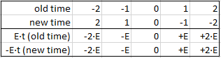
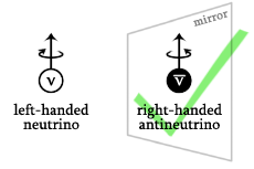 I hope you understand the left- versus right-handed thing. Think, for example, of how the left-circularly polarized wavefunction below would look like in the mirror. Just apply the customary right-hand rule to determine the direction of the angular momentum vector. You’ll agree it will be right-circularly polarized in the mirror, right? That’s why we need the charge conjugation: think of the magnetic moment of a circulating charge! So… Well… I can’t dwell on this too much but – if Maxwell’s equations are to hold – then that world in the mirror must be made of antimatter.

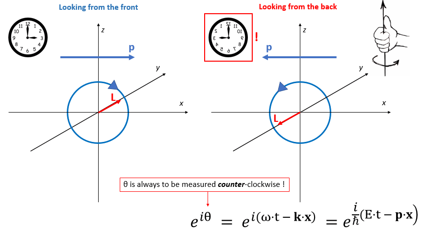 Now, suppose someone else is looking at this from the other side – or just think of yourself going around a full 180° to look at the same thing from the back side. You’ll agree you’ll see the same thing going from right to left (so that’s in the 9 o’clock direction now – or, if our clock is transparent, the 3 o’clock direction of our reversed clock). Likewise, the thing that’s turning around will now go counter-clockwise.
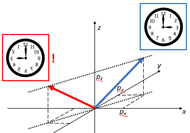
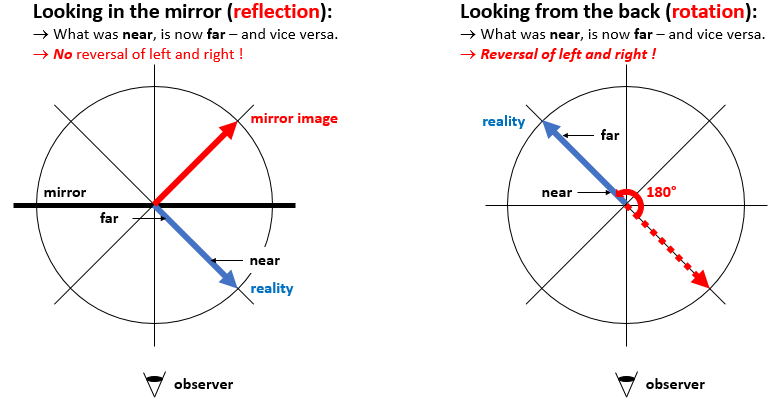
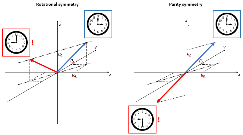
 Now, you know that e–i·(p/ħ)·x and e–i·(p/ħ)·x are each other’s complex conjugate:
 The J·J in the classical formula above is, of course, the equally classical vector dot product, and the formula itself is nothing but Pythagoras’ Theorem in three dimensions. Easy. I just put a + sign in front of the square roots so as to remind you we actually always have two square roots and that we should take the positive one. 🙂
 So now we can apply our classical J·J = Jx2 + Jy2 + Jz2 formula to these quantities by calculating the expected value of J = J·J, which is equal to:
 But… Well… Note those weird angles: we get something close to 24.1° and then another value close to 54.7°. No symmetry here. 😦 The table below gives some more values for larger j. They’re easy to calculate – it’s, once again, just Pythagoras’ Theorem – but… Well… No symmetries here. Just weird values. [I am not saying the formula for these angles is not straightforward. That formula is easy enough: θ = sin-1(m/√[j(j+1)]). It’s just… Well… No symmetry. You’ll see why that matters in a moment.]
 I skipped the half-integer values for j in the table above so you might think they might make it easier to come up with some kind of sensible explanation for the angles. Well… No. They don’t. For example, for j = 1/2 and m = ± 1/2, the angles are ±35.2644° – more or less, that is. 🙂 As you can see, these angles do not nicely cut up our circle in equal pieces, which triggers the obvious question: are these angles really equally likely? Equal angles do not correspond to equal distances on the z-axis (in case you don’t appreciate the point, look at the illustration below).
 That’s why
  The nutation is caused by the gravitational force field, and the nutation movement usually dies out quickly because of dampening forces (read: friction). Now, we don’t think of gravitational fields when analyzing angular momentum in quantum mechanics, and we shouldn’t. But there is something else we may want to think of. There is also a phenomenon which is referred to as free nutation, i.e. a nutation that is not caused by an external force field. The Earth, for example, nutates slowly because of a gravitational pull from the Sun and the other planets – so that’s not a free nutation – but, in addition to this, there’s an even smaller wobble – which is an example of free nutation – because the Earth is not exactly spherical. In fact, the Great Mathematician, Leonhard Euler, had already predicted this, back in 1765, but it took another 125 years or so before an astronomist, Seth Chandler, could finally experimentally confirm and measure it. So they named this wobble
  I am not sure if this approach would solve the problem of our angles and distances – the issue of whether we should think in equally likely angles or equally likely distances along the z-axis, really – but… Well… I’ll let you play with this. Please do send me some feedback if you think you’ve found something. 🙂
 In fact, now that I’ve shown this graph, I should quickly explain it. The three graphs are the spherically symmetric wavefunctions for the first three energy levels. For the first energy level – which is conventionally written as n = 1, not as n = 0 – the amplitude approaches zero rather quickly. For n = 2 and n = 3, there are zero-crossings: the curve passes the r-axis. Feynman calls these zero-crossing radial nodes. To be precise, the number of zero-crossings for these s-states is n − 1, so there’s none for n = 1, one for n = 2, two for n = 3, etcetera.
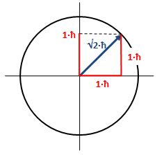 What if l = 2? The magnitude of l is then equal to √[2·(2+1)]·ħ = √6·ħ ≈ 2.4495·ħ. How do we relate that to those “cocked” angles? The values of m now range from -2 to +2, with a unit distance in-between. The illustration below shows the angles. [I didn’t mention ħ any more in that illustration because, by now, we should know it’s our unit of measurement – always.]
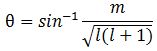 It’s simple but intriguing. Needless to say, the sin −1 function is the inverse sine, also known as the arcsine. I’ve calculated the values for all m for l = 1, 2, 3, 4 and 5 below. The most interesting values are the angles for m = 1 and m = l. As the graphs underneath show, for m = 1, the values start approaching the zero angle for very large l, so there’s not much difference any more between m = ±1 and m = 1 for large values of l. What about the m = l case? Well… Believe it or not, if l becomes really large, then these angles do approach 90°. If you don’t remember how to calculate limits, then just calculate θ for some huge value for l and m. For l = m = 1,000,000, for example, you should find that θ = 89.9427…°. 🙂
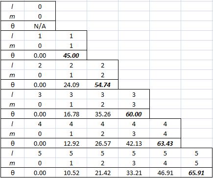
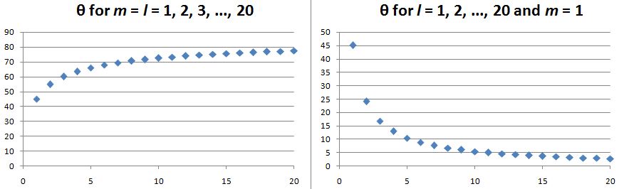 Isn’t this fascinating? I’ve actually never seen this in a textbook – so it might be an original contribution. 🙂 OK. I need to get back to the grind:
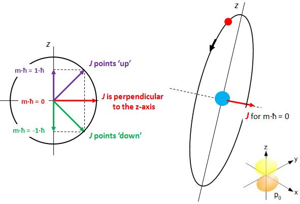

 A more complete table is given below:
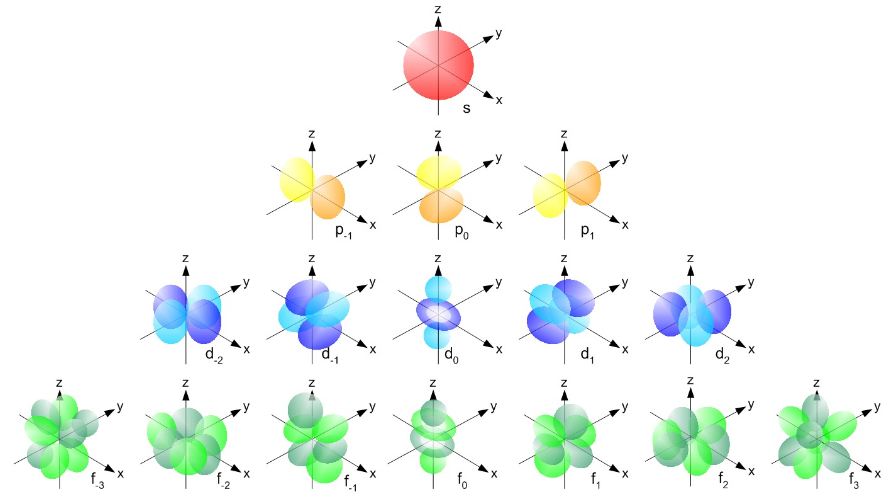 But… Hey! Wait a moment! We only have these Yl,m(θ, φ) functions here. What about Fl(r)?
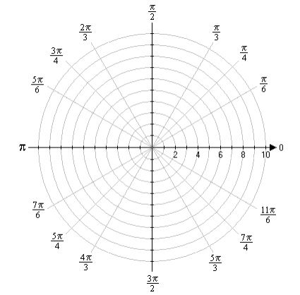
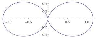
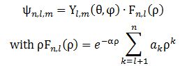
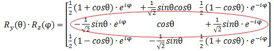
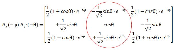
 So far, so good. But what happens if we have two polarizers, set up as shown below, with the optical axis of the first one at an angle θ, which is, say, equal to 30°? Will any light get through?
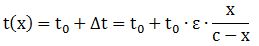 So… This function tells us that the dependent variable is the travel time t, and that it is seen as a function of some independent variable x and some parameters t0, c and ε. My son defined the variable x as the flow (of vehicles) on the road, and c as the capacity of the road. To be precise, he wrote the formula that was to be used for c as follows:
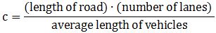 What about a formula for x? Well… He said that was the actual flow of vehicles, but he had no formula for it. As for t0, that was the travel time “at free speed.” Finally, he said ε was a “paramètre de sensibilité de congestion.” Sorry for the French, but that’s the language of his school, which is located in some town in southern Belgium. In English, we might translate it as a congestion sensitivity coefficient. And so that’s what he struggled most with – or so he said.
 Davidson’s function is, quite simply, just nicer and easier than the one above, because the function above is not linear. It could be quadratic (β = 2), or whatever, but surely not linear. In contrast, Davidson’s function is linear and, therefore, easy to fit onto actual traffic data using the simplest of simple linear regression models – and, speaking from experience, most engineers and economists in a real-life job can barely handle even that! 🙂
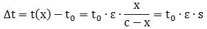 So we have a very simple linear functional form for the extra travel time, and we can easily estimate the actual value of our ε parameter using actual traffic data in a simple linear regression. The data analysis toolkit of MS Excel will do stuff like this – if you have the data, of course – so you don’t need a sophisticated statistical software package here.
 But so what’s the free-flow speed? Is it the maximum speed of my friend’s Maserati -which is like 275 km/h? Well… I don’t think my friend ever drove that fast, so probably not. What else? Think about it. What should we choose here? The obvious choice is the speed limit: 120 km/h, or 90 km/h, or 60 km/h – or whatever. Why? Because you don’t want a ticket, I guess… In any case, let’s analyze that question later. Let’s first look at something else.
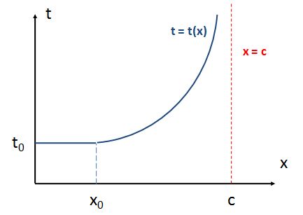 To be specific, if the speed limit is 120 km/h, then – assuming you don’t want to be caught speeding – the minimum travel time will always be equal to 30 seconds per km, even if you’re alone on the highway. Now, as long as the density is less than 45 vehicles per km, you can keep that travel time the same, because you can do your 120 km/h while keeping the safety distance. But if the density increases, above 45 vehicles per km, then stuff starts slowing down because everyone is uncomfortable with the shorter distance between them and the car in front. As the density goes up even more – say, to 60 vehicles per km – we can only do 90 km/h, and so the travel time will then be equal to 40 seconds per km. And then it goes to 90 vehicles per km, so speed slows down to 60 km/h, and so that’s a travel time of 60 seconds per km. Of course, you’re smart – very smart – and so you’ll immediately say this implies that the second section of our graph should be linear too, like this:
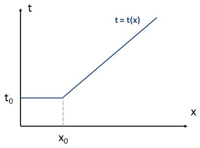 You’re right. But then… Well… That doesn’t work with our limit for x, which is c. As I pointed out, c is an absolute maximum density: you just can’t park any more cars on that highway – unless you fold them up or so. 🙂 So what’s the conclusion? Well… We may think of the Davidson function as a primitive combination of both shapes, as shown below.