An introduction to virtual particles

Pre-script (dated 26 June 2020): Our ideas have evolved into a full-blown realistic (or classical) interpretation of all things quantum-mechanical. In addition, I note the dark force has amused himself by removing some material. So no use to read this. Read my recent papers instead. šŸ™‚

Original post:

We are going toĀ venture beyond quantum mechanics as it is usually understood – covering electromagnetic interactions only. Indeed, all of my posts so far – a bit less than 200, I think šŸ™‚ – were all centered around electromagnetic interactions – with the model of the hydrogen atom as our most precious gem, so to speak.

In this post, we’ll be talking the strong force – perhaps not for the first time but surely for the first time at this level of detail. It’s an entirely different world – as I mentioned in one of my very first posts in this blog. Let me quote what I wrote there:

“The math describing the ‘reality’ of electrons and photons (i.e. quantum mechanics and quantum electrodynamics), as complicated as it is, becomes even more complicated – and, important to note, also much less accurate – when it is used to try to describe the behavior of Ā quarks. Quantum chromodynamics (QCD) is a different world. […]Ā Of course, that should not surprise us, because we’re talking very different order of magnitudes here: femtometers (10–15 m), in the case of electrons, as opposed to attometers (10–18 m)Ā or even zeptometers (10–21Ā m) when we’re talking quarks.”

In fact, the femtometer scale is used to measure the radiusĀ of both protons as well as electrons and, hence, is much smaller than the atomic scale, which is measured in nanometer (1 nm = 10āˆ’9Ā m). The so-called Bohr radius for example, which is a measure for the size of an atom, is measured in nanometer indeed, so that’s a scale that is aĀ millionĀ times larger than the femtometer scale. ThisĀ gapĀ in the scale effectively separates entirely different worlds. In fact, the gap is probably as large a gap as the gap between our macroscopic world and the strange reality of quantum mechanics. What happens at the femtometer scale,Ā really?

The honest answer is: we don’t know, but we do have modelsĀ to describe what happens. Moreover, for want of better models, physicists sort of believe these models are credible. To be precise, we assume there’s a force down there which we refer to as theĀ strongĀ force. In addition, there’s also a weak force. Now, you probably know these forces are modeled asĀ interactionsĀ involving anĀ exchangeĀ ofĀ virtualĀ particles. This may be related to what Aitchison and Hey refer to as the physicist’s “distaste for action-at-a-distance.” To put it simply: if one particle – through some force – influences some other particle, then something must be going on between the two of them.

Of course, now you’ll say that something isĀ effectively going on: there’s the electromagnetic field, right? Yes. But what’s the field? You’ll say: waves. But then you know electromagnetic waves also have a particle aspect. So we’re stuck with this weird theoretical framework: the conceptual distinction between particles and forces, or between particle and field, are not so clear. So that’s what the more advanced theories we’ll be looking at – like quantum field theory – try to bring together.

Note that we’ve been using a lot of confusing and/or ambiguous terms here: according to at least one leading physicist, for example, virtual particles should not be thought of as particles! But we’re putting the cart before the horse here. Let’s go step by step. To better understand the ‘mechanics’ of how the strong and weak interactions are being modeled in physics, most textbooks – including Aitchison and Hey, which we’ll follow here – start by explaining the original ideas as developed by the Japanese physicist Hideki Yukawa, who received a Nobel Prize for his work in 1949.

So what is it all about? As said, the ideasĀ – or theĀ modelĀ as such, so to speak – are more important than Yukawa’s original application, which was to model the force between a proton and a neutron. Indeed, we now explain such force as a force between quarks, and the force carrier is the gluon, which carries the so-calledĀ colorĀ charge. To be precise, the force between protons and neutrons – i.e. the so-called nuclearĀ force – isĀ nowĀ considered to be a rather minorĀ residual force: it’s just what’s left of the actualĀ strong force that binds quarks together. The Wikipedia article on thisĀ has someĀ good text andĀ a really nice animation on this. But… Well… Again, note that we are only interested in theĀ model right now. So how does that look like?

First, we’ve got the equivalent of the electric charge: the nucleon is supposed to have some ‘strong’ charge, which we’ll write as gs. Now you know the formulas for theĀ potentialĀ energy – because of the gravitational force – between two masses, or theĀ potentialĀ energy between two charges – because of the electrostatic force. Let me jot them down once again:

  1. U(r) = –GĀ·MĀ·m/r
  2. U(r) = (1/4πε0)Ā·q1Ā·q2/r

The two formulas are exactly the same. They both assume U = 0 forĀ r → āˆž. Therefore, U(r) is always negative. [Just think of q1Ā and q2Ā as opposite charges, so the minus sign is not explicit – but it is also there!] We know thatĀ U(r)Ā curve will look like the one below: some work (force times distance) is needed to move the two charges some distanceĀ away from each other – from point 1 to point 2, for example. [The distance r is x here – but you got that, right?]potential energy

Now, physics textbooks – or other articles you might find, like on Wikipedia – will sometimes mention that the strong force is non-linear, but that’s very confusing because… Well… The electromagnetic force – or the gravitational force – aren’t linear either: their strength is inversely proportional to the squareĀ of the distance and – as you can see from the formulas for the potential energy – that 1/r factor isn’t linearĀ either. So that isn’t very helpful. In order to further the discussion, I should now write down Yukawa’sĀ hypotheticalĀ formula for the potential energy between a neutron and a proton, which we’ll refer to, logically, as the n-p potential:n-p potentialThe āˆ’gs2Ā factor is, obviously, the equivalent of the q1Ā·q2Ā product: think of the proton and the neutron having equal but opposite ‘strong’ charges. The 1/4Ļ€ factor reminds us of the Coulomb constant:Ā keĀ = 1/4πε0. Note this constant ensures the physical dimensions of both sides of the equation make sense: the dimension of ε0Ā is NĀ·m2/C2, so U(r) is – as we’d expect – expressed in newtonĀ·meter, orĀ joule. We’ll leave the question of the units for gsĀ open – for the time being, that is. [As for the 1/4Ļ€ factor, I am not sure why Yukawa put it there. My best guess is that he wanted to remind us some constant should be there to ensure the units come out alright.]

So, when everything is said and done, the big new thing is the eāˆ’r/a/rĀ factor, which replaces the usual 1/r dependency on distance. Needless to say, e is Euler’s number here –Ā notĀ the electric charge. The two green curves below show what the eāˆ’r/aĀ factor does to the classical 1/r function for aĀ = 1 andĀ aĀ = 0.1 respectively: smaller values forĀ aĀ ensure the curve approaches zero more rapidly. In fact, forĀ aĀ = 1,Ā eāˆ’r/a/rĀ is equal to 0.368 forĀ rĀ = 1, and remains significant for values rĀ that are greater than 1 too.Ā In contrast, forĀ aĀ = 0.1, eāˆ’r/a/rĀ is equal to 0.004579 (more or less, that is) for rĀ = 4 and rapidly goes to zero for all values greater than that.

graph 1graph 2Aitchison and Hey callĀ a, therefore, aĀ range parameter: it effectively defines theĀ rangeĀ in which the n-p potential has a significant value: outside of the range, its value is, for all practical purposes, (close to) zero. Experimentally, this range was established as being more or less equal to r ≤ 2 fm.Ā Needless to say, while this range factor may do its job, it’s obvious Yukawa’s formula for the n-p potential comes across as being somewhat random: what’s the theory behind? There’s none, really. It makes one think of the logistic function: the logistic function fits many statistical patterns, but it is (usually) not obvious why.

Next in Yukawa’s argument is the establishment of an equivalent, for the nuclear force, of the Poisson equation in electrostatics: using theĀ E = ā€“āˆ‡Ī¦ formula, we can re-write Maxwell’s āˆ‡ā€¢EĀ = ρ/ε0Ā equation (aka Gauss’ Law) asĀ āˆ‡ā€¢E =Ā ā€“āˆ‡ā€¢āˆ‡Ī¦Ā = ā€“āˆ‡2Ī¦Ā ā‡”Ā āˆ‡2Φ= –ρ/ε0Ā indeed. The divergenceĀ operatorĀ theĀ āˆ‡ā€¢ operator gives us theĀ volumeĀ density of the flux of E out of an infinitesimal volume around a given point. [You may want to check one of my post on this. The formula becomes somewhat more obvious if we re-write it as āˆ‡ā€¢EĀ·dV = –(ρ·dV)/ε0: āˆ‡ā€¢EĀ·dV is then, quite simply, the flux of E out of the infinitesimally small volume dV, and the right-hand side of the equation says this is given by the product of the charge inside (ρ·dV) and 1/ε0, which accounts for the permittivity of the medium (which is the vacuum in this case).] Of course, you will also remember the āˆ‡Ī¦ notation: āˆ‡ is just the gradient (or vector derivative) of the (scalar) potential Φ, i.e. the electric (or electrostatic) potential in a space around that infinitesimally small volume with charge density ρ. So… Well… The Poisson equation is probably notĀ soĀ obvious as it seems at first (again, checkĀ my post on itĀ on it for more detail) and, yes, that āˆ‡ā€¢ operator – the divergenceĀ operator – is a pretty impressive mathematical beast. However, I must assume you master this topic and move on. So… Well… I must now give you the equivalent of Poisson’s equation for the nuclear force. It’s written like this:Poisson nuclearWhat the heck? Relax. To derive this equation, we’d need to take a pretty complicated dĆ©tour, which we won’t do. [See Appendix G of Aitchison and Grey if you’d want the details.] Let me just point out the basics:

1. The Laplace operator (āˆ‡2) is replaced by one that’s nearly the same: āˆ‡2Ā āˆ’ 1/a2. And it operates on the same concept: a potential, which is a (scalar) function of the position r. Hence, U(r) is just the equivalent of Φ.

2. The right-hand side of the equation involves Dirac’s delta function. Now that’s a weird mathematical beast. Its definition seems to defy what I refer to as the ‘continuum assumption’ in math. Ā I wrote a few things about it in one of my posts on Schrƶdinger’s equationĀ – and I could give you its formula – but that won’t help you very much. It’s just a weird thing. As Aitchison and GreyĀ write, you should just think of the whole expression as a finite range analogueĀ of Poisson’s equation in electrostatics. So it’s only for extremely smallĀ rĀ that the whole equation makes sense. Outside of the range defined by our range parameterĀ a, the whole equation just reduces to 0 = 0 – for all practical purposes, at least.

Now, of course, you know that the neutron and the proton are not supposed to just sit there. They’re also in these sort of intricate dance which – for the electron case – is described by some wavefunction, which we derive as a solution from Schrƶdinger’s equation. So U(r) is going to vary not only in space but also in time and we should, therefore, write it as U(r, t). Now, we will, of course, assume it’s going to vary in space and time as someĀ waveĀ and we may, therefore, suggest some waveĀ equationĀ for it. To appreciate this point, you should review some of the posts I did on waves. More in particular, you may want to review the post I did on traveling fields, in which I showed you the following:Ā if we see an equation like:f8then the function ψ(x, t) must have the following general functional form:solutionAnyĀ function ψ like that will work – so it will be a solution to the differential equation – and we’ll refer to it as a wavefunction. Now, the equation (and the function) is for a wave traveling inĀ one dimension only (x) but the same post shows we can easily generalize to waves traveling in three dimensions. In addition, we may generalize the analyse to includeĀ complex-valuedĀ functions as well. Now, you will still be shocked by Yukawa’s field equation for U(r, t) but, hopefully, somewhat less so after the above reminder on how wave equations generally look like:Yukawa wave equationAs said, you can look up the nitty-gritty in Aitchison and GreyĀ (or in its appendices) but, up to this point, you should be able to sort of appreciate what’s going on without getting lost in it all. Yukawa’s next step – and all that follows – is much more baffling. We’d think U, the nuclear potential, is just some scalar-valued wave, right? It varies in space and in time, but… Well… That’s what classical waves, like water or sound waves, for example do too. So far, so good. However, Yukawa’s next step is to associate aĀ de Broglie-type wavefunction with it. Hence, Yukawa imposesĀ solutions of the type:potential as particleWhat?Ā Yes. It’s a big thing to swallow, and it doesn’t help most physicists refer to U as aĀ force field. A force and the potential that results from it are two different things. To put it simply: theĀ forceĀ on an object isĀ notĀ the same as theĀ workĀ you need to move it from here to there. Force and potential areĀ relatedĀ butĀ differentĀ concepts. Having said that, it sort of make sense now, doesn’t it? If potential is energy, and if it behaves like some wave, then we must be able to associate it with aĀ de Broglie-type particle. This U-quantum, as it is referred to, comes in two varieties, which are associated with the ongoingĀ absorption-emission process that is supposed to take place inside of the nucleus (depicted below):

p + Uāˆ’Ā ā†’ n andĀ n + U+ → p

absorption emission

It’s easy to see that theĀ Uāˆ’Ā andĀ U+Ā particles are just each other’s anti-particle. When thinking about this, I can’t help remembering Feynman, when he enigmatically wrote – somewhere in his Strange Theory of Light and MatterĀ – thatĀ an anti-particle might just be the same particle traveling back in time.Ā In fact, theĀ exchangeĀ here is supposed to happen within aĀ time windowĀ that is so short it allows for the briefĀ violationĀ of the energy conservation principle.

Let’s be more precise and try to find the properties of that mysterious U-quantum. You’ll need to refresh what you know about operators to understand how substituting Yukawa’sĀ de BroglieĀ wavefunction in the complicated-looking differential equation (the waveĀ equation) gives us the following relation between the energy and the momentum of our new particle:mass 1Now, it doesn’t take too many gimmicks to compare this against the relativistically correct energy-momentum relation:energy-momentum relationCombining both gives us the associated (rest) mass of the U-quantum:rest massForĀ aĀ ā‰ˆ 2 fm,Ā mUĀ is about 100 MeV. Of course, it’s always to check the dimensions and calculate stuff yourself. Note the physical dimension of ħ/(aĀ·c) is NĀ·s2/m = kg (just think of the F = mĀ·a formula). Also note that NĀ·s2/m = kg = (NĀ·m)Ā·s2/m2Ā = J/(m2/s2), so that’s the [E]/[c2] dimension.Ā The calculation – and interpretation – is somewhat tricky though: if you do it, you’ll find that:

ħ/(aĀ·c) ā‰ˆ (1.0545718Ɨ10āˆ’34Ā NĀ·mĀ·s)/[(2Ɨ10āˆ’15Ā m)Ā·(2.997924583Ɨ108Ā m/s)] ā‰ˆ 0.176Ɨ10āˆ’27Ā kg

Now, most physics handbooks continue that terrible habit of writing particle weights in eV, rather than using the correct eV/c2Ā unit. So when they write: mUĀ is about 100 MeV, they actually mean to say that it’s 100 MeV/c2. In addition, the eV is notĀ an SI unit. Hence, to get that number, we should first write 0.176Ɨ10āˆ’27Ā kg as some value expressed in J/c2, and then convert the jouleĀ (J) into electronvolt (eV). Let’s do that. First, note that c2Ā ā‰ˆ 9Ɨ1016Ā m2/s2, so 0.176Ɨ10āˆ’27Ā kgĀ ā‰ˆĀ 1.584Ɨ10āˆ’11Ā J/c2. Now we do the conversion from jouleĀ to electronvolt. WeĀ get: (1.584Ɨ10āˆ’11Ā J/c2)Ā·(6.24215Ɨ1018Ā eV/J)Ā ā‰ˆ 9.9Ɨ107Ā eV/c2Ā = 99 MeV/c2.Ā Bingo!Ā So that was Yukawa’s prediction for theĀ nuclear force quantum.

Of course, Yukawa was wrong but, as mentioned above, his ideas are now generally accepted. First note the mass of the U-quantum is quite considerable:Ā 100 MeV/c2Ā is a bit more than 10% of the individual proton or neutron mass (about 938-939 MeV/c2). While theĀ binding energyĀ causes the mass of an atom to be less than the mass of their constituent parts (protons, neutrons and electrons), it’s quite remarkably that the deuterium atom – a hydrogen atom with an extra neutron – has an excess mass of about 13.1 MeV/c2, and a binding energy with an equivalent mass of only 2.2 MeV/c2. So… Well… There’s something there.

As said, this post only wanted to introduce some basic ideas. The current model of nuclear physics is represented by the animation below, which I took from the Wikipedia article on it. The U-quantum appears as the pion here – and it doesĀ notĀ really turn the proton into a neutron and vice versa. Those particles are assumed to be stable. In contrast, it is theĀ quarksĀ that changeĀ colorĀ by exchanging gluons between each other. And we know look at the exchange particle – which we refer to as the pionĀ –Ā between the proton and the neutron as consisting of two quarks in its own right: a quark and a anti-quark. So… Yes… All weird. QCD is just a different world. We’ll explore it more in the coming days and/or weeks. šŸ™‚Nuclear_Force_anim_smallerAn alternative – and simpler – way of representing this exchange of a virtual particle (a neutralĀ pionĀ in this case) is obtained by drawing a so-called Feynman diagram:Pn_scatter_pi0OK. That’s it for today. More tomorrow. šŸ™‚

Some content on this page was disabled on June 20, 2020 as a result of a DMCA takedown notice from Michael A. Gottlieb, Rudolf Pfeiffer, and The California Institute of Technology. You can learn more about the DMCA here:

https://wordpress.com/support/copyright-and-the-dmca/
Some content on this page was disabled on June 20, 2020 as a result of a DMCA takedown notice from Michael A. Gottlieb, Rudolf Pfeiffer, and The California Institute of Technology. You can learn more about the DMCA here:

https://wordpress.com/support/copyright-and-the-dmca/

Reality and perception

It’s quite easy to get lost in all of the math when talking quantum mechanics. In this post, I’d like to freewheel a bit. I’ll basically try to relate the wavefunction we’ve derived for the electron orbitals to the more speculative posts I wrote on how toĀ interpretĀ the wavefunction. So… Well… Let’s go. šŸ™‚

If there is one thing you should remember from all of the stuff I wrote in my previous posts, then it’s that the wavefunction for an electron orbital – ψ(x, t), so that’s a complex-valued function in twoĀ variables (position and time) – canĀ be written as the product of two functions in oneĀ variable:

ψ(x, t) = eāˆ’iĀ·(E/ħ)Ā·tĀ·f(x)

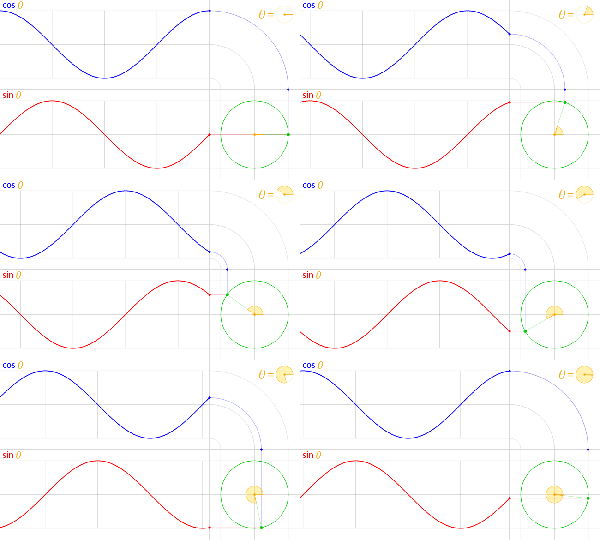
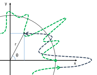
In fact, we wrote f(x) as ψ(x), but I told you how confusing that is: the ψ(x) and ψ(x, t) functions are, obviously,Ā veryĀ different. To be precise,Ā theĀ f(x) = ψ(x) function basically provides some envelope for the two-dimensional eiĪøĀ =Ā eāˆ’iĀ·(E/ħ)Ā·tĀ = cosĪø + iĀ·sinĪøĀ oscillation – as depicted below (Īø = āˆ’(E/ħ)Ā·tĀ = ω·tĀ with ω = āˆ’E/ħ).Circle_cos_sinWhen analyzing this animation – look at the movement of the green, red and blue dots respectively – one cannot miss the equivalence between this oscillation and the movement of a mass on a spring – as depicted below.spiral_sThe eāˆ’iĀ·(E/ħ)Ā·tĀ function just gives us twoĀ springs for the price of one. šŸ™‚ Now, you may want to imagine some kind of elastic medium – Feynman’s famous drum-head, perhaps šŸ™‚ – and you may also want to think of all of this in terms of superimposed waves but… Well… I’d need to review if that’s really relevant to what we’re discussing here, so I’d rather notĀ make things too complicated and stick to basics.

First note that the amplitude of the two linear oscillations above is normalized: the maximum displacement of the object from equilibrium, in the positive or negative direction, which we may denote by x = ±A, is equal to one. Hence, the energy formula is just the sum of the potential and kinetic energy: T + U = (1/2)Ā·A2Ā·m·ω2Ā = (1/2)Ā·m·ω2. But so we haveĀ twoĀ springs and, therefore, the energy in this two-dimensional oscillation is equal to E = 2Ā·(1/2)Ā·m·ω2Ā =Ā m·ω2.

This formula is structurally similar to Einstein’sĀ E = mĀ·c2Ā formula. Hence, one may want to assume that the energy of some particle (an electron, in our case, because we’re discussing electron orbitals here)Ā is just the two-dimensional motion of itsĀ mass. To put it differently, we might also want to think that the oscillating real and imaginary component of our wavefunction each store one halfĀ of the total energy of our particle.

However, the interpretation of this rather bold statement is not so straightforward. First, you should note that the ω in the E =Ā m·ω2Ā formula is an angularĀ velocity, as opposed to the cĀ in theĀ E = mĀ·c2Ā formula, which is a linear velocity. Angular velocities are expressed inĀ radiansĀ per second, while linear velocities are expressed inĀ meterĀ per second. However, while theĀ radianĀ measures an angle, we know it does so by measuring a length. Hence, if our distance unit is 1 m, an angle of 2π rad will correspond to a length of 2π meter, i.e. the circumference of the unit circle. So… Well… The two velocities mayĀ notĀ be so different after all.

There are other questions here. In fact, the other questions are probably more relevant. First, we should note that the ω in the E =Ā m·ω2Ā can take on any value. For a mechanical spring, ω will be a function of (1) the stiffnessĀ of the spring (which we usually denote by k, and which is typically measured in newton (N) per meter) and (2) the mass (m) on the spring. To be precise, we write: ω2Ā = k/m – or, what amounts to the same, ω = √(k/m). Both k and m are variablesĀ and, therefore, ω can really be anything. In contrast, we know that c is a constant: cĀ equalsĀ 299,792,458 meter per second, to be precise. So we have this rather remarkable expression: cĀ = √(E/m), and it is valid for anyĀ particle – our electron, or the proton at the center, or our hydrogen atom as a whole. It is also valid for more complicated atoms, of course. In fact, it is valid forĀ anyĀ system.

Hence, we need to take another look at the energy conceptĀ that is used in our ψ(x, t) = eāˆ’iĀ·(E/ħ)Ā·tĀ·f(x) wavefunction. You’ll remember (if not, youĀ should) that the E here is equal to EnĀ = āˆ’13.6 eV, āˆ’3.4 eV, āˆ’1.5 eV and so on, for nĀ = 1, 2, 3, etc. Hence, this energy concept is rather particular. As Feynman puts it: “The energies are negative because we picked our zero point as the energy of an electron located far from the proton. When it is close to the proton, its energy is less, so somewhat below zero. The energy is lowest (most negative) for n = 1, and increases toward zero with increasing n.”

Now, this is theĀ one and onlyĀ issue I have with the standard physics story. I mentioned it in one of my previous posts and, just for clarity, let me copy what I wrote at the time:

Feynman gives us a rather casual explanation [on choosing a zero point for measuring energy] in one of his very firstĀ LecturesĀ on quantum mechanics, where he writes the following:Ā ā€œIf we have a ā€œconditionā€ which is a mixture of two different states with different energies, then the amplitude for each of the two states will vary with time according to an equation likeĀ aĀ·eāˆ’iωt, with ħ·ω =Ā EĀ = mĀ·c2. Hence, we can write the amplitude for the two states, for example as:

eāˆ’i(E1/ħ)Ā·tĀ and eāˆ’i(E2/ħ)Ā·t

And if we have some combination of the two, we will have an interference. But notice that if we added a constant to both energies, it wouldn’t make any difference. If somebody else were to use a different scale of energy in which all the energies were increased (or decreased) by a constant amount—say, by the amount A—then the amplitudes in the two states would, from his point of view, be:

eāˆ’i(E1+A)Ā·t/ħ and eāˆ’i(E2+A)Ā·t/ħ

All of his amplitudes would be multiplied by the same factor eāˆ’i(A/ħ)Ā·t, and all linear combinations, or interferences, would have the same factor. When we take the absolute squares to find the probabilities, all the answers would be the same. The choice of an origin for our energy scale makes no difference; we can measure energy from any zero we want. For relativistic purposes it is nice to measure the energy so that the rest mass is included, but for many purposes that aren’t relativistic it is often nice to subtract some standard amount from all energies that appear. For instance, in the case of an atom, it is usually convenient to subtract the energy MsĀ·c2, where MsĀ is the mass of all the separate pieces—the nucleus and the electrons—which is, of course, different from the mass of the atom. For other problems, it may be useful to subtract from all energies the amount MgĀ·c2, where MgĀ is the mass of the whole atom in the ground state; then the energy that appears is just the excitation energy of the atom. So, sometimes we may shift our zero of energy by some very large constant, but it doesn’t make any difference, provided we shift all the energies in a particular calculation by the same constant.ā€

It’s a rather long quotation, but it’s important. The key phrase here is, obviously, the following: ā€œFor other problems, it may be useful to subtract from all energies the amount MgĀ·c2, where MgĀ is the mass of the whole atom in the ground state; then the energy that appears is just the excitation energy of the atom.ā€ So that’s what he’s doing when solving Schrƶdinger’s equation. However, I should make the following point here: if we shift the origin of our energy scale, it does not make any difference in regard to theĀ probabilitiesĀ we calculate, but it obviously does make a difference in terms of our wavefunction itself. To be precise, itsĀ densityĀ in time will beĀ veryĀ different. Hence, if we’d want to give the wavefunction someĀ physicalĀ meaning – which is what I’ve been trying to do all along – itĀ doesĀ make a huge difference. When we leave the rest mass of all of the pieces in our system out, we can no longer pretend we capture their energy.

So… Well… There you go. If we’d want to try to interpret our ψ(x, t) = eāˆ’iĀ·(En/ħ)Ā·tĀ·f(x) function as a two-dimensional oscillation of theĀ massĀ of our electron, the energy concept in it – so that’s the EnĀ in it – should include all pieces. Most notably, it should also include the electron’sĀ rest energy, i.e. its energy when it is notĀ in a bound state. This rest energy is equal to 0.511 MeV. […]Ā Read this again: 0.511 mega-electronvolt (106Ā eV), so that’s huge as compared to the tiny energy values we mentioned so far (āˆ’13.6 eV, āˆ’3.4 eV, āˆ’1.5 eV,…).

Of course, this gives us a rather phenomenal order of magnitude for the oscillation that we’re looking at. Let’s quickly calculate it. We need to convert to SI units,Ā of course: 0.511 MeV is about 8.2Ɨ10āˆ’14Ā jouleĀ (J), and so the associated frequencyĀ is equal to ν = E/h = (8.2Ɨ10āˆ’14Ā J)/(6.626Ɨ10āˆ’34 JĀ·s) ā‰ˆ 1.23559Ɨ1020Ā cycles per second. Now, I know such number doesn’t say all that much: just note it’s the same order of magnitude as the frequency of gamma raysĀ and… Well… No. I won’t say more. You should try to think about this for yourself. [If you do,Ā think – for starters – aboutĀ the difference between bosons and fermions: matter-particles are fermions, and photons are bosons. Their nature is very different.]

The correspondingĀ angularĀ frequency is just the same number but multiplied by 2Ļ€ (one cycle corresponds to 2π radiansĀ and, hence, ω = 2π·ν = 7.76344Ɨ1020Ā radĀ per second. Now, if our green dot would be moving around the origin, along the circumference of our unit circle, then its horizontal and/or vertical velocity would approach the same value. Think of it. We have thisĀ eiĪøĀ =Ā eāˆ’iĀ·(E/ħ)Ā·tĀ =Ā ei·ω·tĀ = cos(ω·t) +Ā iĀ·sin(ω·t) function, with ω = E/ħ. So theĀ cos(ω·t) captures the motion along the horizontal axis, while the sin(ω·t) function captures the motion along the vertical axis.Ā Now, the velocity along the horizontalĀ axis as a function of time is given by the following formula:

v(t) = d[x(t)]/dt = d[cos(ω·t)]/dt =Ā āˆ’Ļ‰Ā·sin(ω·t)

Likewise, the velocity along theĀ verticalĀ axis is given byĀ v(t) = d[sin(ω·t)]/dt = ω·cos(ω·t). These are interesting formulas: they show the velocity (v) along one of the two axes is always lessĀ than theĀ angular velocity (ω). To be precise, the velocity vĀ approaches – or, in the limit, is equal to –Ā the angular velocity ω when ω·t is equal to ω·tĀ = 0, π/2, Ļ€ or 3Ļ€/2. So… Well… 7.76344Ɨ1020Ā meterĀ per second!? That’s like 2.6Ā trillionĀ times the speed of light. So that’s not possible, of course!

That’s where theĀ amplitudeĀ of our wavefunction comes in – our envelope functionĀ f(x): the green dot doesĀ notĀ move along the unit circle. The circle is much tinier and, hence, the oscillation shouldĀ notĀ exceed the speed of light. In fact, I should probably try to prove it oscillatesĀ atĀ the speed of light, thereby respecting Einstein’s universal formula:

c = √(E/m)

Written like this – rather than as you know it: E = mĀ·c2Ā – this formula shows the speed of light is just a property of spacetime, just like the ω = √(k/m) formula (or the ω = √(1/LC) formula for a resonant AC circuit) shows that ω, the naturalĀ frequency of our oscillator, is a characteristic of the system.

Am I absolutely certain of what I am writing here? No. My level of understanding of physics is still that of an undergrad. But… Well… It all makes a lot of sense, doesn’t it? šŸ™‚

Now, I said there were a fewĀ obvious questions, and so far I answered only one. The other obvious question is why energy would appear to us as mass in motionĀ in two dimensions only. Why is it an oscillation in a plane? We might imagine a third spring, so to speak, moving in and out from us, right? Also, energyĀ densitiesĀ are measured per unitĀ volume, right?

NowĀ that‘s a clever question, and I must admit I can’t answer it right now. However, I do suspect it’s got to do with the fact that the wavefunction depends on the orientation of our reference frame. If we rotate it, it changes. So it’s like we’ve lost one degree of freedom already, so only two are left. Or think of the third direction as the direction of propagationĀ of the wave. šŸ™‚Ā Also, we should re-read what we wrote about the Poynting vector for the matter wave, or what Feynman wrote about probabilityĀ currents. Let me give you some appetite for that by noting that we can re-writeĀ jouleĀ per cubic meter (J/m3) asĀ newtonĀ perĀ squareĀ meter: J/m3Ā = NĀ·m/m3Ā = N/m2. [Remember: the unit of energy is force times distance. In fact, looking at Einstein’s formula, I’d say it’s kgĀ·m2/s2Ā (mass times a squared velocity), but that simplifies to the same: kgĀ·m2/s2Ā = [N/(m/s2)]Ā·m2/s2.]

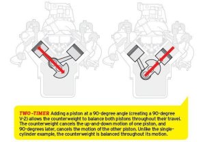
I should probably also remindĀ you that there is no three-dimensional equivalent of Euler’s formula, and the way the kinetic and potential energy of those two oscillations works together is rather unique. Remember I illustrated it with the image of a V-2 engine in previous posts. There is no such thing as a V-3 engine. [Well… There actually is – but not with the third cylinder being positioned sideways.]two-timer-576-px-photo-369911-s-original

But… Then… Well… Perhaps we should think of some weird combination ofĀ twoĀ V-2 engines. The illustration below shows the superposition of twoĀ one-dimensional waves – I think – one traveling east-west and back, and the other one traveling north-south and back. So, yes, we may to think of Feynman’s drum-head again – but combiningĀ two-dimensional waves –Ā twoĀ waves thatĀ bothĀ have an imaginary as well as a real dimension

dippArticle-14

Hmm… Not sure. If we go down this path, we’d need to add a third dimension – so w’d have a super-weird V-6 engine! As mentioned above, the wavefunction does depend on our reference frame: we’re looking at stuff from a certain directionĀ and, therefore, we can only see what goes up and down, and what goes left or right. We can’t see what comes near and what goes away from us. Also think of the particularities involved in measuring angular momentum – or the magnetic moment of some particle. We’re measuring that along one direction only! Hence, it’s probably no use to imagine we’re looking atĀ threeĀ waves simultaneously!

In any case…Ā I’ll let you think about all of this. I do feel I am on to something. I am convinced that my interpretation of the wavefunction as anĀ energy propagationĀ mechanism, or asĀ energy itselfĀ – as a two-dimensional oscillation of mass – makes sense. šŸ™‚

Of course, I haven’t answered oneĀ keyĀ question here: whatĀ isĀ mass? What is that green dot – in reality, that is? At this point, we can only waffle – probably best to just give its standard definition: mass is a measure ofĀ inertia. A resistance to acceleration or deceleration, or to changing direction. But that doesn’t say much. I hate to say that – in many ways – all that I’ve learned so far hasĀ deepenedĀ the mystery, rather than solve it. The more we understand, the less we understand? But… Well… That’s all for today, folks ! Have fun working through it for yourself. šŸ™‚

Post scriptum: I’ve simplified the wavefunction a bit. As I noted in my post on it, the complex exponential is actually equal toĀ eāˆ’iĀ·[(E/ħ)Ā·tĀ āˆ’Ā m·φ], so we’ve got a phase shift because of m, the quantum number which denotes the z-component of the angular momentum. But that’s a minor detail that shouldn’t trouble or worry you here.

Re-visiting electron orbitals (III)

Pre-script (dated 26 June 2020): Our ideas have evolved into a full-blown realistic (or classical) interpretation of all things quantum-mechanical. In addition, I note the dark force has amused himself by removing some material. So no use to read this. Read my recent papers instead. šŸ™‚

Original post:

In my previous post, I mentioned that it wasĀ not so obvious (both from a physicalĀ as well as from aĀ mathematicalĀ point of view) to write the wavefunction for electron orbitals – which we denoted as ψ(x, t), i.e. a function of two variables (or four: one time coordinate and three space coordinates) –Ā as the product of two other functions in one variable only.

[…] OK. The above sentence is difficult to read. Let me write in math. šŸ™‚ It isĀ notĀ so obvious to write ψ(x, t) as:

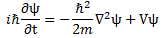
ψ(x, t) = eāˆ’iĀ·(E/ħ)Ā·t·ψ(x)

As I mentioned before, the physicists’ use of the same symbol (ψ, psi) for both the ψ(x, t) and ψ(x) function is quite confusing – because the two functions areĀ veryĀ different:

  • ψ(x, t) is a complex-valued function of twoĀ (real)Ā variables: x and t. OrĀ four, I should say, because xĀ = (x, y, z) – but it’s probably easier to think of x as oneĀ vectorĀ variable – aĀ vector-valued argument, so to speak. And then t is, of course, just aĀ scalarĀ variable. So… Well… A function of twoĀ variables: the position in space (x), and time (t).
  • In contrast, ψ(x) is a real-valuedĀ function ofĀ oneĀ (vector) variable only: x, so that’s the position in space only.

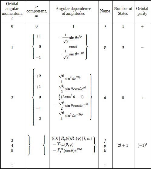
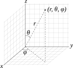
Now you should cry foul, of course: ψ(x) is notĀ necessarilyĀ real-valued. It mayĀ be complex-valued. You’re right.Ā You know the formula:wavefunctionNote the derivation of this formula involved a switch from Cartesian to polar coordinates here, so from xĀ = (x, y, z) to rĀ = (r, Īø, φ), and that the function is also a function of the twoĀ quantum numbersĀ l and m now, i.e. the orbital angular momentum (l) and its z-component (m) respectively. In my previous post(s), I gave you the formulas for Yl,m(Īø, φ) and Fl,m(r) respectively. Fl,m(r) was a real-valued function alright, but the Yl,m(Īø, φ) had that eiĀ·m·φ factor in it. So… Yes. You’re right: the Yl,m(Īø, φ) function is real-valued if – and onlyĀ if – m = 0, in which case eiĀ·m·φ = 1.Ā Let me copy the table from Feynman’s treatment of the topic once again:spherical harmonics 2The Plm(cosĪø) functions are the so-called (associated) Legendre polynomials, and the formula for these functions is rather horrible:Legendre polynomialDon’t worry about it too much: just note the Plm(cosĪø)Ā is aĀ real-valuedĀ function. The point is the following:the ψ(x, t) is a complex-valuedĀ function because – andĀ onlyĀ because – we multiply a real-valued envelope function – which depends on positionĀ only – with eāˆ’iĀ·(E/ħ)Ā·tĀ·eiĀ·m·φ = eāˆ’iĀ·[(E/ħ)Ā·tĀ āˆ’Ā m·φ].

[…]

Please read the above once again and – more importantly – think about it for a while. šŸ™‚ You’ll have to agree with the following:

  • As mentioned in my previous post,Ā the eiĀ·m·φ factor just gives us phase shift: just aĀ re-set of our zero point for measuring time, so to speak, and the whole eāˆ’iĀ·[(E/ħ)Ā·tĀ āˆ’Ā m·φ]Ā factor just disappears when we’re calculating probabilities.
  • The envelope function gives us the basic amplitude – in theĀ classicalĀ sense of the word:Ā the maximum displacement fromĀ theĀ zeroĀ value. And so it’s that eāˆ’iĀ·[(E/ħ)Ā·tĀ āˆ’Ā m·φ]Ā that ensures the whole expression somehow captures the energyĀ of the oscillation.

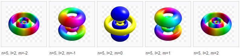
Let’s first look at the envelope function again. Let me copy the illustration forĀ n = 5 and lĀ = 2 from aĀ Wikimedia CommonsĀ article.Ā Note the symmetry planes:

  • Any plane containing theĀ z-axis is a symmetry plane – like a mirror in which we can reflect one half of theĀ shape to get the other half. [Note that I am talking theĀ shapeĀ only here. Forget about the colors for a while – as these reflect the complex phase of the wavefunction.]
  • Likewise, the plane containingĀ bothĀ the x– and the y-axis is a symmetry plane as well.

n = 5

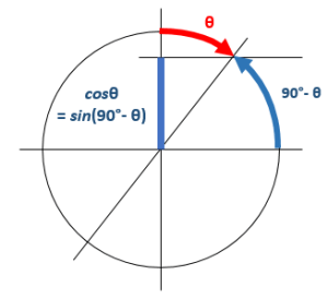
The first symmetry plane – or symmetryĀ line, really (i.e. theĀ z-axis) – should not surprise us, because the azimuthal angle φ is conspicuously absent in the formula for our envelope function if, as we are doing in this article here, we merge theĀ eiĀ·m·φ factor with the eāˆ’iĀ·(E/ħ)Ā·t, so it’s just part and parcel of what the author of the illustrations above refers to as the ‘complex phase’ of our wavefunction.Ā OK. Clear enough – I hope. šŸ™‚ But why is theĀ the xy-plane a symmetry plane too? We need to look at that monstrous formula for the Plm(cosĪø) function here: just note the cosĪø argument in it is being squaredĀ before it’s used in all of the other manipulation. Now, we know that cosĪø = sin(Ļ€/2Ā āˆ’Ā Īø). So we can define someĀ newĀ angle – let’s just call it α – which is measured in the way we’re used to measuring angle, which is notĀ from the z-axis but from the xy-plane. So we write: cosĪø = sin(Ļ€/2Ā āˆ’Ā Īø) = sinα. The illustration below may or may not help you to see what we’re doing here.angle 2So… To make a long story short, we can substitute the cosĪø argument in the Plm(cosĪø) function for sinα = sin(Ļ€/2Ā āˆ’Ā Īø). Now, if the xy-plane is a symmetry plane, then we must find the same value for Plm(sinα) and Plm[sin(āˆ’Ī±)]. Now, that’s not obvious, because sin(āˆ’Ī±) = āˆ’sinα ≠ sinα. However, because the argument in that Plm(x) function is being squared before any other operation (like subtracting 1 and exponentiating the result), it is OK: [āˆ’sinα]2Ā = [sinα]2Ā =Ā sin2α. […] OK, I am sure the geeks amongst my readers will be able to explain this more rigorously. In fact, I hope they’ll have a look at it, because there’s also that dl+m/dxl+mĀ operator, and so you should check what happens with the minus sign there. šŸ™‚

[…] Well… By now, you’re probably totally lost, but the fact of the matter is that we’ve got a beautiful result here. Let me highlight the most significant results:

  • AĀ definiteĀ energy state of a hydrogen atom (or of an electron orbiting around some nucleus, I should say) appears to us as some beautifully shaped orbital – an envelopeĀ function in three dimensions, really – whichĀ has the z-axis – i.e. the vertical axis – as a symmetry line and the xy-plane as a symmetry plane.
  • The eāˆ’iĀ·[(E/ħ)Ā·tĀ āˆ’Ā m·φ]Ā factor gives us the oscillation within the envelope function. As such, it’s this factor that, somehow,Ā captures the energyĀ of the oscillation.

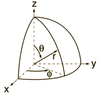
It’s worth thinking about this. Look at the geometry of the situation again – as depicted below. We’re looking at the situation along the x-axis, in the direction of the origin, which is the nucleus of our atom.

spherical

The eiĀ·m·φ factor just gives us phase shift: just aĀ re-set of our zero point for measuring time, so to speak. Interesting, weird – but probably less relevant than the eāˆ’iĀ·[(E/ħ)Ā·tĀ factor, which gives us the two-dimensional oscillation that captures the energy of the state.

Circle_cos_sin

Now, the obvious question is: the oscillation of what, exactly? I am not quite sure but – as I explained in my Deep BlueĀ page – the real and imaginary part of our wavefunction are really like the electric and magnetic field vector of an oscillating electromagnetic field (think of electromagnetic radiation – if that makes it easier). Hence, just like the electric and magnetic field vector represent some rapidly changing forceĀ on a unit charge, the real and imaginary part of our wavefunction must also represent some rapidly changingĀ forceĀ on… Well… I am not quite sure on what though. The unit charge is usually defined as the charge of a proton – rather than an electron – but then forces act on some mass, right? And the massĀ of a proton is hugely different from the mass of an electron. The same electric (or magnetic) force will, therefore, give a hugely different acceleration to both.

So… Well… My guts instinct tells me the real and imaginary part of our wavefunction just represent, somehow, a rapidly changing force on some unit ofĀ mass, but then I am not sure how to define that unit right now (it’s probably notĀ the kilogram!).

Now, there is another thing we should note here: we’re actually sort of de-constructing a rotationĀ (look at the illustration above once again) in two linearly oscillating vectors – one along the z-axis and the other along the y-axis.Ā Hence, in essence, we’re actually talking about something that’s spinning.Ā In other words, we’re actually talking someĀ torqueĀ around the x-axis. In what direction? I think that shouldn’t matter – that we can write E or āˆ’E, in other words, but… Well… I need to explore this further – as should you! šŸ™‚

Let me just add one more note on the eiĀ·m·φ factor. It sort of defines the geometryĀ of the complex phase itself. Look at the illustration below. Click on it to enlarge it if necessary – or, better still, visit the magnificent Wikimedia Commons article from which I get these illustrations. These are the orbitals nĀ = 4 and lĀ = 3. Look at the red hues in particular – or the blue – whatever: focus on one color only, and see how how – for mĀ = ±1, we’ve got one appearance of that color only. For mĀ = ±1, the same color appears at two ends of the ‘tubes’ – or toriĀ (plural of torus), I should say – just to sound more professional. šŸ™‚ For mĀ = ±2, the torus consists of three parts – or, in mathematical terms, we’d say the order of its rotational symmetryĀ is equal to 3.Ā Check that Wikimedia Commons article for higher values ofĀ nĀ andĀ l: the shapes become very convoluted, but the observation holds. šŸ™‚

l = 3

Have fun thinking all of this through for yourself – and please do look at those symmetries in particular. šŸ™‚

Post scriptum: You should do some thinking on whether or not theseĀ mĀ = ±1, ±2,…, ±lĀ orbitals are really different. As I mentioned above, a phase difference is just what it is: a re-set of the t = 0 point. Nothing more, nothing less. So… Well… As far as I am concerned, that’s notĀ aĀ realĀ difference, is it? šŸ™‚ As with other stuff, I’ll let you think about this for yourself.

Some content on this page was disabled on June 17, 2020 as a result of a DMCA takedown notice from Michael A. Gottlieb, Rudolf Pfeiffer, and The California Institute of Technology. You can learn more about the DMCA here:

https://wordpress.com/support/copyright-and-the-dmca/

Some more on symmetries…

In our previous post, we talked a lot about symmetries in space – in a rather playful way. Let’s try to take it further here by doing some more thinking on symmetries inĀ spacetime. This post will pick up some older stuff – from my posts on statesĀ and the related quantum math in November 2015, for example – but that shouldn’t trouble you too much. On the contrary, I actually hope to tie up some loose ends here.

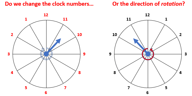
Let’s first review some obvious ideas. Think about the direction of time. On a time axis, time goes from left to right. It will usually be measured from someĀ zeroĀ point – like when we started our experiment or something šŸ™‚ – to some +tĀ point but we may also think of some point in timeĀ beforeĀ ourĀ zeroĀ point, so the minusĀ (āˆ’t)Ā points – the left side of the axis – make sense as well. So the directionĀ of time is clear and intuitive. Now, what does it mean to reverseĀ the direction of time?Ā We need to distinguish two things here: the convention, and… Well… Reality. If we would suddenly decide to reverse the direction in which we measureĀ time, then that’s just another convention. We don’t change reality: trees and kids would still grow the way they always did. šŸ™‚ We would just have to change the numbers on our clocks or, alternatively, the direction ofĀ rotationĀ of the hand(s) of our clock, as shown below. [I only showed the hour hand because… Well… I don’t want to complicate things by introducing twoĀ time units. But adding the minute hand doesn’t make any difference.]

clock problemNow, imagine you’re the dictator who decided to change our time measuring convention. How would youĀ go about it? Would you change the numbers on the clock or the direction of rotation? Personally, I’d be in favor of changing the direction of rotation. Why? Well… First, we wouldn’t have to change expressions such as: “If you are looking north right now, then west is in the 9 o’clock direction, so go there.” šŸ™‚ More importantly, it would align our clocks with the way we’re measuring angles. On the other hand, it would notĀ align our clocks with the way theĀ argument (Īø) of our elementaryĀ wavefunction ψ =Ā aĀ·eāˆ’iĪøĀ =Ā e–iĀ·(EĀ·t – pĀ·x)/ħ is measured, because that’s… Well… Clockwise.

So… What are the implications here? We would need to change t forĀ āˆ’t in our wavefunction as well, right? Yep.Ā Good point. So that’s another convention that would change: we should write our elementary wavefunction now as ψ =Ā aĀ·eiĀ·(EĀ·t – pĀ·x)/ħ. So we would have to re-define Īø as Īø = –EĀ·t + pĀ·x = pĀ·x –EĀ·t. So… Well…Ā Done!

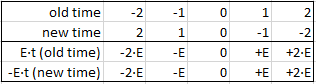
So… Well… What’s next? Nothing. Note that we’re notĀ changing reality here. We’re just adapting our formulas to a new dictatorial convention according to which we should count time from positiveĀ toĀ negativeĀ –Ā like 2, 1, 0, -1, -2 etcetera, as shown below. Fortunately, we can fix allĀ of our laws and formulas in physics byĀ swapping tĀ forĀ -t. So that’s great. No sweat.Ā time reversal

Is that all? Yes. We don’t need to do anything else. We’ll still measure the argument of our wavefunction as an angle, so that’s… Well… After changing our convention, it’s now clockwise. šŸ™‚ Whatever you want to call it: it’s still the sameĀ direction. Our dictator can’t change physical realityĀ šŸ™‚

Hmm… But so we are obviously interested in changing physical reality. I mean… Anyone can become a dictator, right? In contrast, weĀ – enlightened scientists – want to reallyĀ change the world, don’t we? šŸ™‚ So what’s a time reversalĀ in reality? Well… I don’t know… YouĀ tell me. šŸ™‚ We may imagine some movie being played backwards, or trees and kids shrinkingĀ instead of growing,Ā or some bird flying backwards – and I amĀ notĀ talking the hummingbird here. šŸ™‚

Hey!Ā The latter illustration – that bird flying backwards – is probably the better one: if we reverse the direction ofĀ time – in reality, that is – then we should also reverse all directions in space. But… Well… What doesĀ thatĀ mean, really? We need to think in terms of force fields here. A stone that’d be falling must now go back up. Two opposite charges that were goingĀ towardsĀ each other, should now move away from each other. But… My God!Ā Such world cannot exist, can it?

No. It cannot. And we don’t need to invoke the second law of thermodynamics for that. šŸ™‚ None of what happens in a movie that’s played backwards makes sense: a heavy stone doesĀ notĀ suddenly fly up and decelerate upwards. So it is notĀ like the anti-matterĀ world we described in our previous post. No. We can effectively imagine some world in which all charges have been replaced by their opposite: we’d have positiveĀ electrons (positrons) aroundĀ negativelyĀ charged nuclei consisting of antiprotons andĀ antineutrons and, somehow, negativeĀ masses. But Coulomb’s lawĀ would still tell us two opposite charges – q1Ā and –q2Ā , for example – don’t repel butĀ attractĀ each other, with a force that’s proportional to the product of their charges, i.e. q1Ā·(-q2) = –q1Ā·q2. Likewise, Newton’s law of gravitation would still tell us that two masses m1Ā and m2Ā – negative or positive –Ā will attract each other with a force that’s proportional to the product of their masses, i.e. m1Ā·m2Ā = (-m1)Ā·(-m2). If you’d make a movie in the antimatter world, it would look just like any other movie. It would definitelyĀ notĀ look like a movie being played backwards.

In fact, the latter formula – m1Ā·m2Ā = (-m1)Ā·(-m2)Ā – tells us why: we’re not changing anything by putting a minus sign in front of all of our variables, which are time (t), position (x), mass (m)Ā and charge (q). [Did I forget one? I don’t think so.] Hence, the famous CPT TheoremĀ – which tells us that a world in which (1) time is reversed, (2) all charges have been conjugated (i.e. all particles have been replaced by their antiparticles), and (3) all spatial coordinates now have the opposite sign, is entirely possible (because it would obey the same Laws of Nature that we, in ourĀ world, have discovered over the past few hundred years)Ā – is actually nothing but a tautology. Now, I mean that literally: a tautology is aĀ statement that is true by necessity or by virtue of its logical form. Well… That’s the case here: if we flip the signs of allĀ of our variables, we basically just agreed to count or measure everything from positiveĀ toĀ negative. That’s it. Full stop. Such exoticĀ convention is… Well… Exotic, but itĀ cannotĀ change the real world. Full stop.

Of course, this leaves the more intriguing questions entirely open. PartialĀ symmetries. Like time reversal only. šŸ™‚ Or charge conjugation only. šŸ™‚ So let’s think about that.

We know that the world that we see in a mirror mustĀ be made of anti-matter but, apart from that particularity, that world makes sense: if we drop a stone in front of the mirror, the stone in the mirror will drop down too. Two like charges will be seen as repelling each other in the mirror too, and concepts such as kinetic or potential energy look just the same. So time just seems to tick away in both worlds – no time reversal here! – and… Well… We’ve got two CP-symmetrical worlds here, don’t we? We only flipped the sign of the coordinate frame and of the charges. Both are possible, right? And what’s possible must exist, right? Well… Maybe. That’s the next step. Let’s first see if both are possible. šŸ™‚

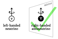
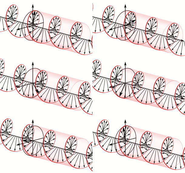
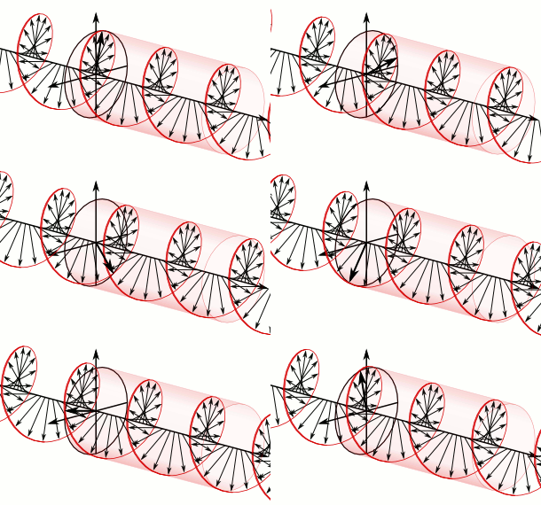
Now, when you’ve read my previous post, you’ll noteĀ that I did notĀ flip theĀ z-coordinate when reflectingĀ my world in the mirror. That’s true. But… Well… That’s entirely beside the point. We could flip the z-axis too and so then we’d have a full parity inversion. [Or parityĀ transformationĀ – sounds more serious, doesn’t it? But it’s only a simple inversion, really.]Ā It really doesn’t matter. The point is: axial vectors have the opposite sign in the mirror world, and so it’s not only about whether or not an antimatter world is possible (it should be, right?): it’s about whether or not the sign reversal of allĀ of those axial vectors makes sense in each and every situation. The illustration below, for example, shows how aĀ left-handedĀ neutrino should be aĀ right-handedĀ antineutrino in the mirror world.right-handed antineutrinoI hope you understand the left- versus right-handed thing. Think, for example, of how the left-circularly polarized wavefunction below would look like in the mirror. Just apply the customary right-hand rule to determine the direction of the angular momentum vector. You’ll agree it will be right-circularly polarized in the mirror, right? That’s why we need the charge conjugation: think of the magnetic moment of a circulating charge! So… Well… I can’t dwell on this too much but – if Maxwell’s equations are to hold – then that world in the mirrorĀ mustĀ be made of antimatter.animation

Now, we know that some processes – in ourĀ world – areĀ notĀ entirely CP-symmetrical. I wrote about this at length in previous posts, so I won’t dwell on these experiments here. The point is: these experiments – which are not easy to understand – lead physicists, philosophers, bloggers and what have you to solemnly state that the world in the mirror cannot reallyĀ exist. And… Well… They’re right. However, I think their observations are beside the point.Ā Literally.

So… Well… I would just like to make a very fundamentalĀ philosophical remark about all those discussions. My point is quite simple:

We should realize that the mirror world andĀ ourĀ world are effectively separated by the mirror. So we should notĀ be looking at stuff inĀ the mirror fromĀ our perspective, because that perspective is well… OutsideĀ of the mirror. A different world. šŸ™‚ In my humble opinion,Ā the valid point of reference would be the observerĀ inĀ the mirror, like the photographer in the image below. Now note the following: if theĀ realĀ photographer, on this side of the mirror, would have a left-circularly polarized beam in front of him, then theĀ imaginaryĀ photographer, on theĀ otherĀ side of the mirror, would see theĀ mirrorĀ image of this left-circularly polarized beam as a left-circularly polarized beam too. šŸ™‚ I know that sounds complicated but re-read it a couple of times and – I hope – you’ll see the point. If you don’t… Well… Let me try to rephrase it: the point is that the observer inĀ the mirrorĀ would be seeingĀ ourĀ world – just the same laws and what have you, all makes sense!Ā – but he would see ourĀ worldĀ inĀ hisĀ world, so he’d see it in the mirror world. šŸ™‚

Mirror

Capito? If you would actually be living inĀ the mirror world, then all the things you would seeĀ inĀ the mirror world would make perfectly sense. But you would be living inĀ the mirror world. You would notĀ look at itĀ from outside, i.e. from the other side of the mirror.Ā In short, I actually think the mirror world does exist – but in the mirror only. šŸ™‚ […] I am, obviously, joking here. Let me be explicit: ourĀ world is our world, and I think those CP violations in Nature are telling us that it’s the onlyĀ realĀ world. The other worlds exist in our mind only – or in some mirror. šŸ™‚

Post scriptum: I know theĀ Die HardĀ philosophers among you will now have an immediate rapid-backfire question. [Hey – I just invented a new word, didn’t I? AĀ rapid-backfireĀ question. Neat.] How would the photographerĀ inĀ the mirror look atĀ ourĀ world? The answer to that question is simple: symmetry! He (or she) would think it’s a mirror world only.Ā HisĀ world andĀ ourĀ world would be separated by the same mirror. So… What are the implications here?

Well… That mirror is only a piece of glass with a coating. We made it. Or… Well… Some man-made company made it. šŸ™‚Ā So… Well… If you think that observer in the mirror – I am talking about that imageĀ of the photographer in that picture above now – would actually exist, then… Well… Then you need to be aware of the consequences: the corollary of hisĀ existence is thatĀ youĀ doĀ notĀ exist. šŸ™‚ And… Well… No. I won’t say more. If you’re reading stuff like this, then you’re smart enough to figure it out for yourself. We live inĀ oneĀ world. Quantum mechanics tells us theĀ perspective on that worldĀ mattersĀ veryĀ much – amplitudes are different in different reference frames – but… Well… Quantum mechanics – or physics in general – doesĀ notĀ give us many degrees of freedoms. None, really. It basically tells us the world we live in is the only world that’sĀ possible, really. But… Then… Well… That’s just because physics… Well… When everything is said and done, it’s just mankind’s drive to ensure our perceptionĀ of the Universe lines up with… Well… What weĀ perceiveĀ it to be. 😦 or šŸ™‚ Whatever your appreciation of it. Those Great Minds did an incredible job. šŸ™‚

Symmetries and transformations

In my previous post, I promised to do something on symmetries. Something simple but then… Well… YouĀ know how it goes: one question always triggers another one. šŸ™‚

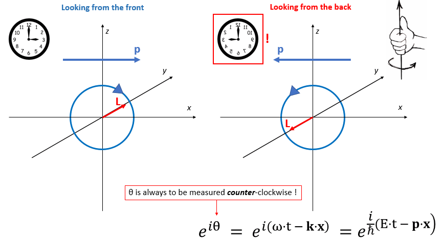
Look at the situation in the illustration on the left below. We suppose we have somethingĀ realĀ going on there: something is moving from left to right (so that’s in the 3 o’clock direction), and then something else is going aroundĀ clockwise (so that’s notĀ the direction in which we measure angles (which also include the argumentĀ Īø of our wavefunction), because that’s alwaysĀ counter-clockwise, as I note at the bottom of the illustration). To be precise, we should note that the angular momentum here is all about the y-axis, so the angular momentum vector L points in the (positive) y-direction. We get that direction from the familiar right-hand rule, which is illustrated in the top right corner.

mirrorNow, suppose someone else is looking at this from the other side – or just think of yourself going around a full 180° to look at the same thing from the back side. You’ll agree you’ll see the same thing going fromĀ rightĀ toĀ left (so that’s in theĀ 9 o’clock direction now – or, if our clock is transparent, the 3 o’clock direction of our reversed clock). Likewise, the thing that’s turning around will now go counter-clockwise.

Note that both observers – so that’s me and that other person (or myself after my walk around this whole thing) – use a regular coordinate system, which implies the following:

  1. We’ve got regular 90° degree angles between our coordinates axes.
  2. Our x-axis goes from negative to positive from left to right, and our y-axis does the same going away from us.
  3. We also both define our z-axis using, once again, the ubiquitous right-hand rule, so our z-axis points upwards.

So we have two observers looking at the same realityĀ – some linearĀ as well as someĀ angularĀ momentum – but from opposite sides. And so we’ve got a reversal of both the linear as well as the angular momentum. NotĀ in reality, of course, because we’re looking at the same thing. But weĀ measureĀ it differently. Indeed, if we use the subscripts 1 and 2 to denote the measurements in the two coordinate systems, we find that p2Ā = –p1.Ā Likewise, we also find that L2Ā = –L1.

Now, when you see these two equations, youĀ will probably not worry aboutĀ thatĀ p2Ā = –p1Ā equation – although you should, because it’s actually only valid for this rather particular orientation of the linear momentum (I’ll come back to that in a moment). It’s the L2Ā = –L1Ā equation which should surprise you most. Why? Because you’ve always been told there is a bigĀ difference between (1)Ā realĀ vectors (aka polar vectors), like the momentumĀ p, or the velocityĀ v, or the force F,Ā and (2)Ā pseudo-vectors (aka axial vectors), like the angularĀ momentumĀ L. You may also remember how to distinguish between the two:Ā if you change theĀ directionĀ of the axes of your reference frame, polar vectors will change sign too, as opposed to axial vectors: axial vectors do notĀ swap sign if we swap the coordinate signs.

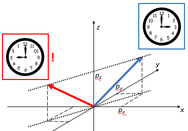
So… Well… How does that work here? In fact, what we should ask ourselves is: why does that notĀ work here? Well… It’s simple, really. We’re not changing the direction of the axes here. Or… Well… Let me be more precise: we’re only swapping the sign of the x– and y-axis. We didĀ notĀ flip the z-axis. So we turned things around, but we didn’t turn them upside down. It makes a huge difference. Note, for example, that if all of the linear momentum would have been in the z-direction only (so ourĀ p vector would have been pointing in the z-direction, and in the z-direction only), it wouldĀ notĀ swap sign. The illustration below shows what really happens with the coordinates of some vector when we’re doing aĀ rotation. It’s, effectively, only theĀ x– andĀ y-coordinates that flip sign.reflection symmetry

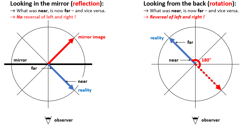
It’s easy to see that thisĀ rotation about the z-axis here preserves our deep sense of ‘up’ versus ‘down’, but that it swaps ‘left’ for ‘right’, and vice versa. Note that this is notĀ a reflection. We areĀ notĀ looking at some mirror world here. The difference between a reflection (a mirror world) and a rotation (the real world seen from another angle) is illustrated below. It’s quite confusing but, unlike what you might think, a reflection does not swap left for right. It does turn things inside out, but that’s what a rotation does as well: near becomes far, and far becomes near.difference between reflection and rotation

Before we move on, let me say a few things about theĀ mirror worldĀ and, more in particular, about the obvious question: could it possiblyĀ exist? Well… What do you think? Your first reaction might well be: “Of course! What nonsense question! We just walk around whatever it is that we’re seeing – or, what amounts to the same, we just turn it around – and there it is: that’s the mirror world, right? So of course it exists!” Well… No. That’sĀ notĀ the mirror world. That’s just theĀ realĀ world seen from the opposite direction, and that world… Well… That’s just the real world. šŸ™‚Ā The mirror world is, literally, the worldĀ in the mirrorĀ – like the photographer in the illustration below. We don’t swap left for right here: some object going from left to right in the real world is still going from left to right in the mirror world!MirrorOf course, you may now involve the photographer in the picture above and observe – note that you’re now an observer of the observer of the mirror šŸ™‚ – that, if he would move his left arm in the real world, the photographer in the mirror world would be moving his right arm. But… Well… No. You’re saying that because you’re nowĀ imaging that you’re the photographer in the mirror world yourself now, who’s looking at the real world from inside, so to speak. So you’ve rotated the perspective in your mindĀ and you’re saying it’s his right arm because you imagineĀ yourself to be the photographer in the mirror.Ā We usually do that because… Well… Because we look in a mirror every day, right? So we’re used to seeing ourselves that way and we always think it’s us we’re seeing. šŸ™‚ However, the illustration above is correct: the mirrorĀ world only swaps near for far, and far for near, so it only swaps the sign of the y-axis.

So the questionĀ isĀ relevant: could the mirror world actually exist? What we’re reallyĀ asking here is the following: can we swap the sign of oneĀ coordinate axisĀ only in all of our physical laws and equations and… Well… Do we then still get the same laws and equations? Do we get the same Universe – because that’s what those laws and equations describe? If so, our mirror world can exist. If not, then not.

Now,Ā I’ve done a post on that, in which I explain that mirror world can only exist if it would consist of anti-matter. So if our real world and the mirror world would actually meet, they would annihilate each other. šŸ™‚ But that post is quite technical. Here I want to keep it veryĀ simple: I basically only want to show what the rotationĀ operation implies for the wavefunction. There is no doubt whatsoever that the rotatedĀ world exists. In fact, the rotated world is just ourĀ world. WeĀ walk around some object, or we turn it around, but so we’re still watching the same object. So we’re not thinking about the mirror world here. We just want to know how things look like when adopting some other perspective.

So, back to the starting point: we just have two observers here, who look at the same thing but from opposite directions. Mathematically, this corresponds to a rotation of our reference frameĀ aboutĀ the z-axis of 180°. Let me spell out – somewhat more precisely – what happens to the linear and angular momentum here:

  1. The direction of the linear momentum in the xy-plane swaps direction.
  2. The angular momentum about the y-axis, as well as about the x-axis, swaps direction too.

Note that the illustration only shows angular momentum about the y-axis, but you can easily verify the statement about the angular momentum about theĀ x-axis. In fact, the angular momentum aboutĀ anyĀ line in theĀ xy-plane will swap direction.

Of course, theĀ x-, y-, z-axes in the other reference frame are different than mine, and so I should give them a subscript, right? Or, at the very least, write something like x’, y’, z’, so we have a primedĀ reference frame here,Ā right? Well… Maybe. Maybe not. Think about it. šŸ™‚ A coordinate system is just a mathematical thing… Only the momentum is real… Linear or angular… Equally real… And then Nature doesn’t care about our position, does it? So… Well… No subscript needed, right? Or… Well… What do youĀ think?Ā šŸ™‚

It’s just funny, isn’t it? It looks like we can’t really separate reality and perception here. Indeed, note how ourĀ p2Ā = –p1Ā and L2Ā = –L1Ā equations already mix reality with how we perceive it. It’s the same thingĀ in realityĀ but the coordinates of p1Ā and L1 are positive, while the coordinates of p2Ā and L2Ā are negative. To be precise, these coordinates will look like this:

  1. p1Ā = (p, 0, 0) and L1 =Ā (0, L, 0)
  2. p2Ā = (āˆ’p, 0, 0) and L1 =Ā (0, āˆ’L, 0)

So are they two different things or are they not? šŸ™‚ Think about it. I’ll move on in the meanwhile. šŸ™‚

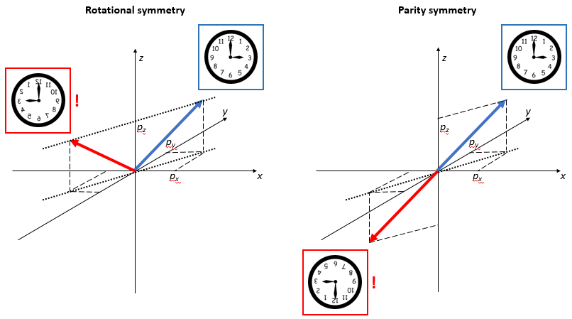
Now, you probably know a thing or two about parityĀ symmetry, orĀ P-symmetry: if if we flip the sign of all coordinates, then we’ll still find the same physical laws, like F = mĀ·a and what have you. [It works for all physical laws, including quantum-mechanical laws – except those involving theĀ weakĀ force (read: radioactive decay processes).] But so here we are talking rotational symmetry. That’s notĀ the same as P-symmetry. If we flip the signs ofĀ allĀ coordinates, we’re also swapping ‘up’ for ‘down’, so we’re not only turning around, but we’re also getting upside down. The difference betweenĀ rotational symmetry and P-symmetry is shown below.up and down swap

As mentioned, we’ve talked about P-symmetry at length in other posts, and you can easilyĀ googleĀ a lot more on that. The question we want to examine here – just as a fun exercise – is the following:

How does that rotationalĀ symmetry work for a wavefunction?

TheĀ very first illustration in this post gave you the functional form of theĀ elementaryĀ wavefunction Ā eiĪø = eiĀ·(EĀ·t – pĀ·x)/ħ. We should actually use a bold typeĀ xĀ = (x, y, z) in this formula but we’ll assume we’re talking something similar to that p vector: something moving in the x-direction only – or in the xy-planeĀ only. TheĀ z-component doesn’t change.Ā Now, you know that we can reduce allĀ actualĀ wavefunctions to some linear combination of such elementary wavefunctions by doing a FourierĀ decomposition, so it’s fine to look at the elementaryĀ wavefunction only – so we don’t make it too complicated here. Now think of the following.

The energy E in theĀ eiĪø = eiĀ·(EĀ·t – pĀ·x)/ħ function is a scalar, so it doesn’t have any direction and we’ll measure it the same from both sides – as kinetic or potential energy or, more likely, by adding both. But… Well… Writing eiĀ·(EĀ·t – pĀ·x)/ħ or eiĀ·(EĀ·t +Ā pĀ·x)/ħ is not the same, right? No, it’s not. However, think of it as follows: we won’t be changing the direction of time, right? So it’s OK to notĀ change the sign of E. In fact, we can re-write the two expressions as follows:

  1. eiĀ·(EĀ·t – pĀ·x)/ħ = eiĀ·(E/ħ)Ā·tĀ·e–iĀ·(p/ħ)Ā·x
  2. ei·(E·t + p·x)/ħ = ei·(E/ħ)·t·ei·(p/ħ)·x

The first wavefunction describes some particle going in the positiveĀ x-direction, while the second wavefunction describes some particle going in the negative x-direction, so… Well… That’s exactlyĀ what we see in those two reference frames, so there is no issue whatsoever. šŸ™‚ It’s just… Well… I just wanted to show the wavefunctionĀ doesĀ look different too when looking at something from another angle.

So why am I writing about this? Why am I being fussy? Well.. It’s just to show you that those transformationsĀ are actually quite natural – just as natural as it is to see some particle go in one direction in one reference frame and see it go in the other in the other. šŸ™‚ It also illustrates another point that I’ve been trying to make: the wavefunction is somethingĀ real. It’s not just a figment of our imagination. The real and imaginary part of our wavefunction have a precise geometrical meaning – and I explained what that might be in my more speculative posts, which I’ve brought together in the Deep BlueĀ page of this blog. But… Well… I can’t dwell on that here because… Well… You should read that page. šŸ™‚

The point to note is the following: weĀ doĀ have different wavefunctions in different reference frames, but these wavefunctions describe the same physical reality, and they alsoĀ do respect the symmetries we’d expect them to respect, except… Well… TheĀ laws describing theĀ weakĀ force don’t, butĀ I wrote about that a veryĀ long time ago, and it wasĀ notĀ in the context of trying to explain the relatively simple basic laws of quantum mechanics. šŸ™‚ If you’re interested, you should check out my post(s) on that or, else, just googleĀ a bit. It’s really exciting stuff, but not something that will help you much to understand the basics, which is what we’re trying to do here. šŸ™‚

The second point to note is that thoseĀ transformationsĀ of the wavefunction – or of quantum-mechanical statesĀ –Ā which we go through when rotating our reference frame, for example – are really quite natural. There’s nothing special about them. We had such transformations in classical mechanics too! But… Well… Yes, I admit they doĀ lookĀ complicated. But then that’s why you’re so fascinated and why you’re reading this blog, isn’t it? šŸ™‚

Post scriptum: It’s probably useful to be somewhat more precise on all of this. You’ll remember we visualized the wavefunction in some of our posts using the animation below. It uses a left-handed coordinate system, which is rather unusual but then it may have been made with a software which uses a left-handed coordinate system (like RenderMan, for example). Now the rotating arrow at the center moves with time and gives us the polarization of our wave. Applying our customary right-handĀ rule,you can see this beam is left-circularly polarized. [I know… It’s quite confusing, but just go through the motions here and be consistent.]AnimationNow, you know that e–iĀ·(p/ħ)Ā·x and e–iĀ·(p/ħ)Ā·xĀ are each other’s complex conjugate:

  1. e–iĀ·kĀ·xĀ =Ā cos(kĀ·x) +Ā iĀ·sin(kĀ·x)
  2. e–iĀ·kĀ·xĀ =Ā cos(-kĀ·x) +Ā iĀ·sin(-kĀ·x) = cos(kĀ·x) āˆ’Ā iĀ·sin(kĀ·x)

Their real part – the cosine function – is the same, but the imaginary part – the sine function – has the opposite sign.Ā So, assuming the direction of propagation is, effectively, the x-direction, then what’s the polarization of the mirror image? Well… The wave will now go from right to left, and its polarization… Hmm…Ā Well… What?Ā 

Well… If you can’t figure it out, then just forget about those signs and just imagine you’re effectively looking at the same thingĀ from the backside. In fact, if you have a laptop, you can push the screen down and go around your computer. šŸ™‚ There’s no shame in that. In fact, I did that just to make sure I am notĀ talking nonsense here. šŸ™‚ If you look at this beam from the backside, you’ll effectively see it go from right to left – instead of from what you see on this side, which is a left-to-right direction. And as for its polarization… Well… The angular momentum vector swaps direction too but the beam is stillĀ left-circularly polarized. So… Well… That’s consistent with what we wrote above. šŸ™‚ The real world is real, and axial vectors are as real as polar vectors. This realĀ beam will only appear to beĀ right-circularly polarizedĀ in a mirror. Now, as mentioned above, that mirror world is notĀ ourĀ world. If it would exist – in some other Universe – then it would be made up of anti-matter. šŸ™‚

So… Well… Might it actually exist? Is there some other world made of anti-matter out there? I don’t know. We need to think about that reversal of ‘near’ and ‘far’ too: as mentioned, a mirror turns things inside out, so to speak. So what’s the implication of that? When we walk aroundĀ something – or do aĀ rotationĀ – then the reversal between ‘near’ and ‘far’ is something physical: we go near to what was far, and we go away from what was near. But so how would we get into our mirror world, so to speak? We may say that thisĀ anti-matter world in the mirror is entirely possible, but then how would we get there? We’d need to turn ourselves, literally, inside out – like short of shrink to the zero point and then come back out of it to do that parity inversion along our line of sight. So… Well… I don’t see that happen, which is why I am a fan of the One World hypothesis. šŸ™‚ SoĀ IĀ thinkĀ the mirror world is just what it is: the mirror world. Nothing real. But… Then… Well… What doĀ youĀ think? šŸ™‚

Quantum-mechanical magnitudes

As I was writing about those rotations in my previous postĀ (on electron orbitals), I suddenly felt I should do some more thinking on (1) symmetries and (2) the concept of quantum-mechanicalĀ magnitudesĀ of vectors. I’ll write about the first topic (symmetries) in some other post. Let’s first tackle the latter concept. Oh… And for those I frightened with my last post… Well… ThisĀ should really be an easy read. More of a short philosophical reflection about quantum mechanics. Not a technical thing. Something intuitive. At least I hope it will come out that way. šŸ™‚

First, you should note that the fundamental idea that quantities like energy, or momentum, may be quantized is a very natural one. In fact, it’s what the early Greek philosophers thought about Nature. Of course, while the idea of quantization comes naturally to us (I think it’s easier to understand than, say, the idea of infinity), it is, perhaps,Ā notĀ so easy to deal with itĀ mathematically. Indeed, most mathematical ideas – like functions and derivatives – are based on what I’ll loosely refer to asĀ continuum theory. So… Yes, quantization does yield some surprising results, like that formula for the magnitude of some vector J:Magnitude formulasThe JĀ·J in the classical formula above is, of course, the equally classical vector dot product, and the formula itself is nothing but Pythagoras’ Theorem in three dimensions. Easy. I just put a + sign in front of the square roots so as to remind you we actually always have twoĀ square roots and that we should take the positive one. šŸ™‚

I will now show you how we get that quantum-mechanical formula. The logic behind it is fairly straightforward but, at the same time… Well… You’ll see. šŸ™‚ We know that a quantum-mechanical variable – like the spin of an electron, or the angular momentum of an atom – is not continuous butĀ discrete: it will have some valueĀ mĀ = j,Ā j-1,Ā j-2, …, -(j-2), -(j-1), –j.Ā OurĀ jĀ here is the maximumĀ value of the magnitude of the component of our vector (J) in the direction of measurement, which – as you know – is usually written as Jz. Why? Because we will usually choose our coordinate system such that ourĀ z-axis is aligned accordingly. šŸ™‚ Those values j,Ā j-1,Ā j-2, …, -(j-2), -(j-1), –j are separated by one unit. That unit would be Planck’s quantum of action ħ ā‰ˆ 1.0545718Ɨ10āˆ’34Ā NĀ·mĀ·s – by the way, isn’t it amazing we can actually measure such tiny stuff in some experiment? šŸ™‚ – ifĀ JĀ would happen to be the angular momentum, but the approach here is more general – actionĀ can express itself in various ways šŸ™‚ – soĀ the unit doesn’t matter: it’s just the unit, so that’s just one. šŸ™‚ It’s easy to see that this separation implies jĀ must be some integer or half-integer. [Of course, now you might think the values of a series like 2.4, 1.4, 0.4, -0.6, -1.6 are also separated by one unit, but… Well… That would violate the most basic symmetry requirement so… Well… No. Our jĀ has to be an integer or a half-integer. Please also note that the number of possible values for mĀ is equal toĀ 2j+1, as we’ll use that in a moment.]

OK. You’re familiar with this by now and so I should not repeat the obvious. To make things somewhat more real, let’s assumeĀ jĀ = 3/2, so mĀ =Ā  3/2, 1/2, -1/2 or +3/2. Now, we don’t know anything about the system and, therefore, these four values are all equally likely. Now, you may notĀ agree with this assumption but… Well… You’ll have to agree that, at this point, you can’t come up with anything else that would make sense, right? It’s just like a classical situation: JĀ might point in any direction, so we have to give allĀ anglesĀ an equal probability.Ā [In fact, I’ll show you – in a minute or so – that you actually have a point here: we should think some more about this assumption – but so that’s for later. I am asking you to just go along with this story as for now.]

So theĀ expectedĀ value ofĀ JzĀ is E[Jz] is equal to E[Jz] = (1/4)Ā·(3/2)+(1/4)Ā·(1/2)+(1/4)Ā·(-1/2)+(1/4)Ā·(-3/2) = 0. Nothing new here. We just multiply probabilities with all of the possible values to get an expected value. So we get zero here because our values are distributed symmetrically around the zero point. No surprise. Now, to calculate a magnitude, we don’t need JzĀ but Jz2. In case you wonder, that’s what this squaring business is all about: we’re abstracting away from the directionĀ and so we’re going to squareĀ both positive as well as negative values to then add it all up and take a square root.Ā Now, the expected value of Jz2Ā is equal to E[Jz] = (1/4)Ā·(3/2)2+(1/4)Ā·(1/2)2+(1/4)Ā·(-1/2)2+(1/4)Ā·(-3/2)2Ā = 5/4 = 1.25. Some positiveĀ value.

You may note that it’s a bit larger than the average of the absoluteĀ value of our variable, which is equal to (|3/2|+|1/2|+|-1/2|+|-3/2|)/4 = 1, but that’s just because the squaring favors larger values šŸ™‚ Also note that, of course, we’d also get some positive value if JzĀ would be a continuous variable over the [-3/2, +3/2] interval, but I’ll let youĀ thinkĀ about whatĀ positive value we’d get for Jz2Ā assuming JzĀ is uniform distributed over the [-3/2, +3/2] interval, because that calculation is actually notĀ so straightforward as it may seem at first. In any case, these considerations are not very relevant to our story here, so let’s move on.

Of course, ourĀ z-direction was random, and so we get the same thing for whatever direction. More in particular, we’ll also get it for theĀ x– andĀ y-directions: E[Jx] = E[Jy] = E[Jz] = 5/4. Now, at this point it’s probably good to give you a more generalized formula for these quantities. I think you’ll easily agree to the following one:magnitude squared formulaSo now we can apply our classical JĀ·J =Ā Jx2Ā +Ā Jy2Ā +Ā Jz2Ā formula to these quantities by calculating the expected value of J =Ā JĀ·J, which is equal to:

E[JĀ·J] = E[Jx2] + E[Jy2] + E[Jz2] = 3Ā·E[Jx2] = 3Ā·E[Jy2] = 3Ā·E[Jz2]

You should note we’re making use of the E[XĀ +Ā Y] = E[X]+ E[Y] property here: the expected value of the sum of two variables is equal to the sum of the expected values of the variables, and you should also note this is true even if the individual variables would happen to be correlated – which might or might not be the case. [What do you think is the case here?]

For jĀ = 3/2, it’s easy to see we get E[JĀ·J] = 3Ā·E[Jx] = 3Ā·5/4 = (3/2)Ā·(3/2+1) = jĀ·(j+1). We should now generalize this formula for other values of j,Ā  which is notĀ so easy… Hmm… It obviously involves some formula for a series, and I am not good at that… So… Well… I just checked if it was true forĀ jĀ = 1/2 andĀ jĀ = 1 (please check thatĀ at least for yourself too!) and then I just believe the authorities on thisĀ for all other values of j. šŸ™‚

Now, in a classicalĀ situation, we knowĀ thatĀ JĀ·J product will be the same for whatever direction JĀ wouldĀ happen to have, and so its expected value will be equal to its constantĀ value JĀ·J. So we can write:Ā E[JĀ·J] = JĀ·J.Ā So… Well… That’s why we write what we wrote above:Magnitude formulas

Makes sense, no? E[J·J] = E[Jx2+Jy2+Jz2] = E[Jx2]+E[Jy2]+E[Jz2] = j·(j+1) = J·J = J2, so J = +√[j(j+1)], right?

Hold your horses, man!Ā Think! What are we doing here, really? We didn’t calculate all that much above. We only found that E[Jx2]+E[Jy2]+E[Jz2] = E[Jx2+Jy2+Jz2] = Ā jĀ·(j+1). So what?Ā Well… That’s notĀ a proof thatĀ theĀ JĀ vector actually exists.

Huh?Ā 

Yes. That JĀ vector might just be some theoretical concept. When everything is said and done, all we’ve been doing – or at least, weĀ imaginedĀ we did – is thoseĀ repeated measurements of Jx,Ā JyĀ andĀ JzĀ here – or whatever subscript you’d want to use, like JĪø,φ, for example (the example is notĀ random, of course) – and so, of course, it’s only natural that we assume these things are the magnitude of the component (in the direction of measurement)Ā of someĀ realĀ vector that is out there, but then… Well… Who knows? Think of what we wrote about the angular momentum in our previous post on electron orbitals. WeĀ imagine – or do like to think – thatĀ there’s some angular momentum vector JĀ outĀ there, which we think of as being “cocked” at some angle, so its projection onto the z-axis gives us those discrete values forĀ mĀ which, for jĀ = 2, for example, are equal to 0, 1 or 2 (and -1 and -2, of course) – like in the illustration below. šŸ™‚cocked angle 2But… Well… NoteĀ those weird angles: we get something close to 24.1° and then another value close to 54.7°. No symmetry here. 😦 The table below gives some more values for largerĀ j. They’re easy to calculate – it’s, once again, just Pythagoras’ Theorem – but… Well… No symmetries here. Just weird values. [I amĀ notĀ saying the formula for these angles isĀ notĀ straightforward. That formula is easy enough:Ā Īø = sin-1(m/√[j(j+1)]). It’s just… Well… No symmetry. You’ll see why that matters in a moment.]CaptureI skipped the half-integer values forĀ jĀ in the table above so you might think they might make it easier to come up with some kind of sensible explanation for the angles. Well… No. They don’t. For example, forĀ jĀ = 1/2 and m = ± 1/2, the angles are ±35.2644° – more or less, that is. šŸ™‚ As you can see, these angles doĀ notĀ nicely cut up our circle in equal pieces, which triggers the obvious question: are these angles really equallyĀ likely? Equal angles doĀ notĀ correspond to equal distances on theĀ z-axis (in case you don’t appreciate the point, look at the illustration below). Ā angles distance

So… Well… Let me summarize the issue on hand as follows: the idea of the angle of the JĀ vector being randomly distributed is not compatible with the idea of those JzĀ values being equally spaced and equally likely. The latter idea – equally spaced and equally likelyĀ JzĀ values – relates to different possible statesĀ of the system being equally likely, so… Well… It’s just a different idea. 😦

Now there is another thing which we should mention here. The maximum value of theĀ z-component of ourĀ JĀ vector is always smaller thanĀ that quantum-mechanical magnitude, and quite significantly so for smallĀ j, as shown in the table below. It is only for larger values ofĀ jĀ that the ratio of the two starts to converge to 1. For example, forĀ jĀ = 25, it is about 1.02, so that’s only 2% off.Ā convergenceThat’s why physicists tell us that, in quantum mechanics, the angular momentum is never “completely along the z-direction.” It is obvious that this actually challenges the ideaĀ of a veryĀ precise direction in quantum mechanics, but then that shouldn’t surprise us, does it? After, isn’t this what the Uncertainty Principle is all about?

DifferentĀ states, rather than differentĀ directions… And then Uncertainty because… Well… Because of discrete variables that won’t split in the middle. Hmm… 😦

Perhaps. Perhaps I should just accept all of this and go along with it… But… Well… I am really not satisfied here, despite Feynman’s assurance that that’s OK:Ā ā€œUnderstanding of these matters comes very slowly, if at all. Of course, one does get better able to know what is going to happen in a quantum-mechanical situation—if that is what understanding means—but one never gets a comfortable feeling that these quantum-mechanical rules are ‘natural’.ā€

I do want to get that comfortable feeling – onĀ some sunny day, at least. šŸ™‚Ā And so I’ll keep playing with this, until… Well… Until I give up. šŸ™‚ In the meanwhile, if you’dĀ feel you’ve got some better or some more intuitiveĀ explanation for all of this, please do let me know. I’d be very grateful to you. šŸ™‚

Post scriptum: Of course, we would all want to believe thatĀ JĀ somehow exists because… Well… We want to explainĀ those states somehow, right? I, for one, am not happy with being told to just accept things and shut up. So let me add some remarks here. First, you may think that the narrative above should distinguish between polar and axial vectors. You’ll remember polar vectors are theĀ realĀ vectors, like a radius vectorĀ r, or a force F, or velocity or (linear) momentum.Ā Axial vectors (also known as pseudo-vectors) are vectors like the angular momentum vector: we sort ofĀ constructĀ them from… Well… From realĀ vectors. The angular momentum L, for example, is the vector crossĀ product of the radius vector rĀ and the linear momentum vector p: we write L = rƗp.Ā In that sense, they’re a figment of our imagination. But then… What’s real and unreal? The magnitude of L, for example, does correspond to something real, doesn’t it? And its direction does give us the direction of circulation, right? You’re right.Ā Hence, I think polar and axial vectors are both real – in whatever sense you’d want to define real. Their reality is just different, and that’s reflected in their mathematical behavior: if you change theĀ directionĀ of the axes of your reference frame, polar vectors will change sign too, as opposed to axial vectors: they don’t swap sign. They do something else, which I’ll explain in my next post, where I’ll be talking symmetries.

But let us, for the sake of argument, assume whatever I wrote about those angles applies to axialĀ vectors only. Let’s be even more specific, and say it applies to the angular momentum vector only. If that’s the case, we may want to think of aĀ classicalĀ equivalent for the mentioned lack of a precise direction: free nutation. It’s a complicated thing – even more complicated than the phenomenon ofĀ precession, which we should be familiar with by now. Look at the illustration below (which I took from an article of a physics professor from Saint Petersburg), which shows both precession as well as nutation. Think of the movement of a spinning top when you release it: its axis will, at first, nutateĀ around the axis of precession, before it settles in a more steady precession.nutationThe nutation is caused by the gravitational force field, and the nutation movement usually dies out quickly because ofĀ dampeningĀ forces (read: friction). Now, we don’t think of gravitational fields when analyzing angular momentum in quantum mechanics, and we shouldn’t. But there is something else we may want to think of. There is also a phenomenon which is referred to asĀ free nutation, i.e. a nutation that isĀ notĀ caused by an external force field. The Earth, for example, nutates slowly because of a gravitational pull from the Sun and the other planets – so that’sĀ notĀ a free nutation – but, in addition to this, there’s an even smaller wobble – whichĀ isĀ an example of free nutation – because the Earth is not exactly spherical. In fact, the Great Mathematician, Leonhard Euler, had already predicted this, back in 1765, but it took another 125 years or so before an astronomist, Seth Chandler, could finally experimentally confirm and measure it. So they named this wobble the Chandler wobble (Euler already has too many things named after him). šŸ™‚

Now I don’t have much backup here –Ā none, actually šŸ™‚ – but why wouldn’t we imagine our electron would also sort of nutate freely because of… Well… Some symmetric asymmetry – something like the slightly elliptical shape of our Earth. šŸ™‚ We may then effectively imagine the angular momentum vector as continually changing direction between a minimum and a maximum angle – something like what’s shown below, perhaps, between 0 and 40 degrees. Think of it as a rotation within a rotation, or an oscillation within an oscillation – or a standing wave within a standing wave. šŸ™‚wobblingI am not sure if this approach would solve the problem of our angles and distances – the issue of whether we should think in equally likelyĀ angles or equally likelyĀ distancesĀ along the z-axis, really – but… Well… I’ll let you play with this. Please do send me some feedback if you think you’ve found something. šŸ™‚

Whatever your solution is, it is likely to involve the equipartition theorem and harmonics, right? Perhaps we can, indeed, imagine standing waves within standing waves, and then standing waves within standing waves. How far can we go? šŸ™‚

Post scriptum 2: When re-reading this post, I was thinking I should probably do something with the following idea. If we’ve got a sphere, and we’re thinking of some vector pointing to some point on theĀ surfaceĀ of that sphere, then we’re doing something which is referred to as point picking on the surface of a sphere, and the probability distributions – as a function of the polar and azimuthal anglesĀ Īø and φ – are quite particular. See the article on the Wolfram site on this, for example. I am not sure if it’s going to lead to some easy explanation of the ‘angle problem’ we’ve laid out here but… Well… It’s surely an element in the explanation. The key idea here is shown in the illustration below: if the direction of our momentum in three-dimensional space is really random, there may still be more of a chance of an orientation towards the equator, rather than towards the pole. So… Well… We need to study the math of this. šŸ™‚ But that’s for later.density

The Aharonov-Bohm effect

Pre-script (dated 26 June 2020): Our ideas have evolved into a full-blown realistic (or classical) interpretation of all things quantum-mechanical. In addition, I note the dark force has amused himself by removing some material. So no use to read this. Read my recent papers instead. šŸ™‚

Original post:

This title sounds very exciting. It is – or was, I should say – one of these things I thought I would never ever understand, until I started studying physics, that is. šŸ™‚

Having said that, there is – incidentally – nothing very special about the Aharonov-Bohm effect. As Feynman puts it: “The theory was known from the beginning of quantum mechanics in 1926. […] The implication was there all the time, but no one paid attention to it.”

To be fair, he also admits the experiment itself – provingĀ the effect – is “very, very difficult”, which is why the first experiment that claimed to confirm the predicted effect was set up in 1960 only. In fact, some claim the results of that experiment were ambiguous, and that it was only in 1986, with the experiment of Akira Tonomura, that the Aharonov-Bohm effect was unambiguously demonstrated. So what is it about?

In essence, it proves the realityĀ of the vector potential—and of the (related) magnetic field. What do we mean with a realĀ field? To put it simply, aĀ realĀ field cannotĀ act on some particle from a distance through some kind of spooky ‘action-at-a-distance’: real fields must be specified at the position of the particle itselfĀ and describe what happens there. Now you’ll immediately wonder: so what’s aĀ non-real field? Well… Some field that does act through some kind of spookyĀ ‘action-at-a-distance.’ As for an example… Well… I can’t give you one because we’ve only been discussing real fields so far. šŸ™‚

So it’s about what a magnetic (or an electric) field does in terms influencing motion and/or quantum-mechanical amplitudes. In fact, we discussed this matter Ā quite a while ago (check my 2015 post on it). Now, I don’t want to re-write that post, but let me just remind you of the essentials. The twoĀ equations for the magnetic field (B) in Maxwell’s set of four equations (the two others specify the electric fieldĀ E) are: (1)Ā āˆ‡ā€¢B = 0 and (2)Ā c2āˆ‡Ć—B = j/ε0Ā + āˆ‚E/ āˆ‚t. Now, you can temporarily forget about the second equation, but you should note that the āˆ‡ā€¢BĀ = 0 equation is alwaysĀ true (unlike theĀ āˆ‡Ć—EĀ = 0 expression, which is true for electrostatics only, when there are no moving charges). So it says that theĀ divergenceĀ of B is zero,Ā always.

Now, from our posts on vector calculus, you may or may not remember that the divergence of the curl of a vector field is always zero. We wrote:Ā divĀ (curlĀ A) = āˆ‡ā€¢(āˆ‡Ć—A) = 0, always. Now, there is another theorem that we can now apply, which says the following: if the divergence of a vector field, say D, is zero – so if āˆ‡ā€¢D = 0, thenĀ D will be theĀ curl of some other vector fieldĀ C, so we can write:Ā D =Ā āˆ‡Ć—C. When we now apply this to ourĀ āˆ‡ā€¢BĀ = 0 equation, we can confidently state the following:Ā 

If āˆ‡ā€¢BĀ = 0, then there is anĀ A such that B =Ā āˆ‡Ć—A

We can also write this as follows: āˆ‡Ā·B = āˆ‡Ā·(āˆ‡Ć—A) = 0 and, hence, B =Ā āˆ‡Ć—A.Ā Now, it’s this vector field AĀ that is referred to as the (magnetic)Ā vectorĀ potential, and so that’s what we want to talk about here. As a start, it may be good to write out all of the components of ourĀ B =Ā āˆ‡Ć—A vector:

formula for B

In that 2015 post, I answered the question as to why we’d need this new vector field in a way that wasn’t very truthful: I just said that, in many situations, it would beĀ more convenient – from a mathematical point of view, that is – toĀ first findĀ A, and then calculate the derivatives above to get B.

Now, Feynman says the following about this argument in his LectureĀ on the topic: “It is true that in many complex problems it is easier to work withĀ A, but it would be hard to argue that this ease of technique would justify making you learn about one more vector field. […] We have introducedĀ AĀ because it does have an important physical significance: it is a real physical field.”Ā Let us follow his argument here.

Quantum-mechanical interference effects

Let us first remind ourselves of the quintessential electron interference experiment illustrated below. [For a much more modern rendering of this experiment, check out the Ā Tout Est QuantiqueĀ videoĀ on it. It’s much more amusing than my rather dry exposĆ© here, but it doesn’t give you the math.]

interference

We have electrons, all of (nearly) the same energy, which leave the source – one by one – and travel towards a wall with two narrow slits. Beyond the wall is a backstop with a movable detector which measures the rate, which we call I, at which electrons arrive at a small region of the backstop at the distance x from the axis of symmetry. The rate (or intensity)Ā IĀ is proportional to the probability that an individual electron that leaves the source will reach that region of the backstop. This probability has the complicated-looking distribution shown in the illustration, which we understand is due to the interference of two amplitudes, one from each slit. So we associate the two trajectoriesĀ with two amplitudes, which Feynman writes as A1eiΦ1Ā and A2eiΦ2Ā respectively.

As usual, Feynman abstracts away from the time variable here because it is, effectively, not relevant: the interference pattern depends on distances and angles only. Having said that, for a good understanding, we should – perhaps – write our two wavefunctions as A1ei(ωt + Φ1)Ā and A2ei(ωt + Φ2)Ā respectively. The point is: we’ve gotĀ twoĀ wavefunctions – one for each trajectory – even if it’s only one electron going through the slit: that’s the mystery of quantum mechanics. šŸ™‚ We need to add these waves so as to get the interference effect:

R = A1ei(ωt + Φ1)Ā +Ā A2ei(ωt + Φ2)Ā = [A1eiΦ1Ā +Ā A2eiΦ2]Ā·eiωt

Now, we know we need to take the absoluteĀ squareĀ of this thing to get the intensity – or probability (before normalization). The absolute square of a product, is the product of the absolute squares of the factors, and we also know that the absolute square of any complex number is just the product of the same number with its complex conjugate. Hence, the absolute square of the eiωtĀ factor is equal to |eiωt|2Ā = eiωtāˆ™e–iωtĀ = e0Ā = 1. So the time-dependent factor doesn’t matter: that’s why we can always abstract away from it. Let us now take the absolute square of theĀ [A1eiΦ1Ā +Ā A2eiΦ2] factor, which we can write as:

|R|2Ā = |A1eiΦ1Ā +Ā A2eiΦ2|2Ā = (A1eiΦ1Ā +Ā A2eiΦ2)Ā·(A1e–iΦ1Ā +Ā A2e–iΦ2)

= A12Ā + A22Ā + 2Ā·A1Ā·A2Ā·cos(Φ1āˆ’Ī¦2) = A12Ā + A22Ā + 2Ā·A1Ā·A2Ā·cosĪ“ with Ī“ = Φ1āˆ’Ī¦2

OK. This is probably going a bit quick, but you should be able to figure it out, especially when remembering that eiΦ +Ā e–iΦ = 2Ā·cosΦ and cosΦ = cos(āˆ’Ī¦). The point to note is that the intensity is equal to the sum of the intensities of both waves plus a correction factor, which is equal to 2Ā·A1Ā·A2Ā·cos(Φ1āˆ’Ī¦2) and, hence, ranges from āˆ’2Ā·A1Ā·A2Ā to +2Ā·A1Ā·A2. Now, it takes a bit of geometrical wizardry to be able to write the phase difference Ī“ = Φ1āˆ’Ī¦2Ā as

Ī“ = 2π·a/Ī» = 2π·(x/L)Ā·d/Ī»

—but it can be done. šŸ™‚ Well… […] OK. šŸ™‚ Let me quickly help you here by copying another diagram from Feynman – one he uses to derive the formula for the phase difference on arrival between the signals from two oscillators.Ā A1Ā andĀ A2Ā are equal here (A1Ā =Ā A2Ā = A) so that makes the situation below somewhat simpler to analyze. However, instead, we have the added complication of a phase difference (α) at the origin – which Feynman refers to as an intrinsic relative phase.Ā triangle

When we apply the geometry shown above to our electron passing through the slits, we should, of course, equate α to zero.Ā For the rest, the picture is pretty similar as the two-slit picture. The distanceĀ aĀ in the two-slit – i.e. the difference in the path lengths for the two trajectories of our electron(s) – is, obviously, equal to the dĀ·sinĪø factor in the oscillator picture. Also, because L is huge as compared toĀ x, we may assume that trajectory 1 and 2 are more or less parallel and, importantly, that the triangles in the picture – small and large – are rectangular. Now, trigonometry tells us that sinĪø is equal to the ratio of the opposite side of the triangle and the hypotenuse (i.e. the longest side of the rectangular triangle). The opposite side of the triangle is xĀ and, becauseĀ xĀ is very, veryĀ small as compared to L, we may approximate the length of the hypotenuse with L. [I know—a lot of approximations here, but… Well… Just go along with it as for now…] Hence, we can equate sinĪø to x/L and, therefore, aĀ =Ā dĀ·x/L. Now we need to calculate the phase difference. How many wavelengths do we have inĀ a? That’s simple:Ā a/Ī», i.e. the total distance divided by the wavelength. Now these wavelengths correspond to 2π·a/Ī» radiansĀ (one cycle corresponds to one wavelength which, in turn, corresponds to 2Ļ€ radians). So we’re done. We’ve got the formula: Ī“ = Φ1āˆ’Ī¦2Ā = 2π·a/Ī» = 2π·(x/L)Ā·d/Ī».

Huh?Ā Yes. Just think about it. I need to move on.Ā The point is: when xĀ is equal to zero, the two waves are in phase, and the probability will have a maximum. When Ī“ = Ļ€, then the waves are out of phase and interfere destructivelyĀ (cosĻ€ = āˆ’1), so the intensity (and, hence, the probability) reaches a minimum.Ā 

So that’s pretty obvious – or shouldĀ be pretty obvious if you’ve understood some of the basics we presented in this blog. We now move to the non-standard stuff, i.e. the Aharonov-Bohm effect(s).

Interference in the presence of an electromagnetic field

In essence, the Aharonov-Bohm effect is nothing special: it is just a law –Ā twoĀ laws, to be precise – that tells us how theĀ phaseĀ of our wavefunction changes because of the presence of a magnetic and/or electric field. As such, it isĀ notĀ very different from previous analyses and presentations, such as those showing how amplitudes are affected by a potential āˆ’ such as an electric potential, or a gravitational field, or a magnetic fieldĀ āˆ’ and how they relate to a classical analysis of the situation (see, for example, my November 2015 post on this topic). If anything, it’s just a more systematic approach to the topic and – importantly – an approach centered around the use of the vector potential A (and the electric potential Φ). Let me give you the formulas:

f1

f2

The first formula tells us thatĀ the phase of the amplitude for our electron (or whatever charged particle) to arrive at some location via some trajectory is changed by an amount that is equal to the integral of the vector potential along the trajectory times the charge of the particle over Planck’s constant.Ā I know that’s quite a mouthful but just read it a couple of times.

The second formula tells us that, if there’s an electrostatic field, it will produce a phase change given by the negative of theĀ timeĀ integral of the (scalar) potential Φ.

These two expressions – taken together – tell us what happens for any electromagnetic field, static or dynamic. In fact, they are really the (two) law(s) replacing the FĀ =Ā q(EĀ +Ā vƗB) expression in classical mechanics.

So how does it work? Let me further follow Feynman’s treatment of the matter—which analyzes what happens when we’d have some magnetic field in the two-slit experiment (so we assume there’s no electric field: we only look at some magnetic field). We said Φ1Ā was the phase of the wave along trajectory 1, and Φ2Ā was the phase of the wave along trajectory 2. WithoutĀ magnetic field, that is, so B = 0. Now, the (first) formula above tells us that, when the field is switched on, the newĀ phases will be the following:

f3

f4

Hence, the phaseĀ differenceĀ Ī“ = Φ1āˆ’Ī¦2Ā will now be equal to:

f5

Now, we can combine the two integrals into one that goes forward along trajectory 1 and comes back along trajectory 2. We’ll denote this path as 1-2 and write the new integral as follows:

f6

Note that we’re using a notation here which suggests that the 1-2 path isĀ closed, which is… Well… Yet another approximation of the Master. In fact, his assumption that the new 1-2 path is closed proves to be essential in the argument that follows the one we presented above, in which he shows that the inherent arbitrariness in our choiceĀ of a vector potential function doesn’t matter, but… Well… I don’t want to get too technical here.

Let me conclude this post by noting we can re-write our grand formula above in terms of the flux of the magnetic field B:

f7

So… Well… That’s it, really. I’ll refer you to Feynman’s Lecture on this matter for a detailed description of the 1960 experiment itself, which involves a magnetized iron whisker that acts like a tiny solenoid—small enough to match the tiny scale of the interference experiment itself. I must warn you though: there is a rather long discussion in that LectureĀ on the ‘reality’ of the magnetic and the vector potential field which – unlike Feynman’s usual approach to discussions like this – is rather philosophical and partially misinformed, as it assumes there is zeroĀ magnetic field outside of a solenoid. That’s true for infinitely long solenoids, but notĀ true for real-life solenoids: if we have someĀ A, then we must also have some B, and vice versa. Hence, if the magnetic field (B) is a real field (in the sense that it cannotĀ act on some particle from a distance through some kind of spooky ‘action-at-a-distance’), then the vector potentialĀ A is an equally real field—and vice versa. Feynman admits as much as he concludes his rather lengthy philosophical excursion with the following conclusion (out of which I already quoted one line in my introduction to this post):

“This subject has an interesting history. The theory we have described was known from the beginning of quantum mechanics in 1926. The fact that the vector potential appears in the wave equation of quantum mechanics (called the Schrƶdinger equation) was obvious from the day it was written. That it cannot be replaced by the magnetic field in any easy way was observed by one man after the other who tried to do so. This is also clear from our example of electrons moving in a region where there is no field and being affected nevertheless. But because in classical mechanics A did not appear to have any direct importance and, furthermore, because it could be changed by adding a gradient, people repeatedly said that the vector potential had no direct physical significance—that only the magnetic and electric fields are ā€œrealā€ even in quantum mechanics. It seems strange in retrospect that no one thought of discussing this experiment until 1956, when Bohm and Aharonov first suggested it and made the whole question crystal clear. The implication was there all the time, but no one paid attention to it. Thus many people were rather shocked when the matter was brought up. That’s why someone thought it would be worthwhile to do the experiment to see if it was really right, even though quantum mechanics, which had been believed for so many years, gave an unequivocal answer. It is interesting that something like this can be around for thirty years but, because of certain prejudices of what is and is not significant, continues to be ignored.”

Well… That’s it, folks! Enough for today! šŸ™‚

Some content on this page was disabled on June 16, 2020 as a result of a DMCA takedown notice from The California Institute of Technology. You can learn more about the DMCA here:

https://wordpress.com/support/copyright-and-the-dmca/
Some content on this page was disabled on June 16, 2020 as a result of a DMCA takedown notice from The California Institute of Technology. You can learn more about the DMCA here:

https://wordpress.com/support/copyright-and-the-dmca/
Some content on this page was disabled on June 16, 2020 as a result of a DMCA takedown notice from The California Institute of Technology. You can learn more about the DMCA here:

https://wordpress.com/support/copyright-and-the-dmca/
Some content on this page was disabled on June 16, 2020 as a result of a DMCA takedown notice from The California Institute of Technology. You can learn more about the DMCA here:

https://wordpress.com/support/copyright-and-the-dmca/
Some content on this page was disabled on June 16, 2020 as a result of a DMCA takedown notice from The California Institute of Technology. You can learn more about the DMCA here:

https://wordpress.com/support/copyright-and-the-dmca/
Some content on this page was disabled on June 16, 2020 as a result of a DMCA takedown notice from The California Institute of Technology. You can learn more about the DMCA here:

https://wordpress.com/support/copyright-and-the-dmca/
Some content on this page was disabled on June 16, 2020 as a result of a DMCA takedown notice from The California Institute of Technology. You can learn more about the DMCA here:

https://wordpress.com/support/copyright-and-the-dmca/
Some content on this page was disabled on June 16, 2020 as a result of a DMCA takedown notice from The California Institute of Technology. You can learn more about the DMCA here:

https://wordpress.com/support/copyright-and-the-dmca/
Some content on this page was disabled on June 16, 2020 as a result of a DMCA takedown notice from The California Institute of Technology. You can learn more about the DMCA here:

https://wordpress.com/support/copyright-and-the-dmca/

An interpretation of the wavefunction

This is my umpteenth post on the same topic. 😦 It is obvious that this search for a sensible interpretation is consuming me. Why? I am not sure. Studying physics is frustrating. As a leading physicist puts it:

“TheĀ teaching of quantum mechanics these days usuallyĀ follows the same dogma: firstly, the student is told about the failure of classical physics atĀ the beginning of the last century; secondly, the heroic confusions of the founding fathersĀ are described and the student is given to understand that no humble undergraduate studentĀ could hope to actually understand quantum mechanics for himself; thirdly, a deus exĀ machina arrives in the form of a set of postulates (the Schrƶdinger equation, the collapseĀ of the wavefunction, etc); fourthly, a bombardment of experimental verifications is given,Ā so that the student cannot doubt that QM is correct; fifthly, the student learns how toĀ solve the problems that will appear on the exam paper, hopefully with as little thought asĀ possible.”

That’s obviously not the way we want to understand quantum mechanics. [With we,Ā I mean, me, of course, and you, if you’re reading this blog.]Ā Of course, that doesn’t mean I don’t believe Richard Feynman, one of the greatest physicists ever, when he tells us no one, including himself, understands physics quite the way we’dĀ likeĀ to understand it. Such statements should not prevent us from tryingĀ harder. So let’s look for betterĀ metaphors.Ā The animation below shows the two components of the archetypal wavefunction – a simple sine and cosine. They’re the same function actually, but their phases differ by 90 degrees (Ļ€/2).

circle_cos_sin

It makes me think of a V-2 engine with the pistons at a 90-degree angle. Look at the illustration below, which I took from a rather simple article on cars and engines that has nothing to do with quantum mechanics. Think of the moving pistons as harmonic oscillators, like springs.

two-timer-576-px-photo-369911-s-original

We will also think of theĀ center of each cylinder as the zero point: think of that point as a point where – if we’re looking at one cylinder alone – the internal and external pressure balance each other, so the piston would not move… Well… If it weren’t for the other piston, because the second piston isĀ not at the centerĀ when the first is. In fact, it is easy to verify and compare the following positions of both pistons, as well as the associated dynamics of the situation:

Piston 1

Piston 2

Motion of Piston 1

Motion Piston 2

Top

Center

Compressed air will push piston down

Piston moves down against external pressure

Center

Bottom

Piston moves down against external pressure

External air pressure will push piston up

Bottom

Center

External air pressure will push piston up

Piston moves further up and compresses the air

Center

Top

Piston moves further up and compresses the air

Compressed air will push piston down

When the pistons move, their linear motion will be described by a sinusoidal function: a sine or a cosine. In fact, the 90-degree V-2 configuration ensures that the linear motion of the two pistons will be exactly the same, except for a phase difference of 90 degrees. [Of course, because of the sideways motion of the connecting rods, our sine and cosine function describes the linear motion only approximately, but you can easily imagine the idealizedĀ limit situation. If not, check Feynman’s description of the harmonic oscillator.]

The question is: if we’d have a set-up like this, two springs – or two harmonic oscillators – attached to a shaft through a crank, would this really work as a perpetuum mobile? We obviously talk energyĀ being transferred back and forth between the rotating shaft and the moving pistons… So… Well… Let’s model this: the totalĀ energy, potentialĀ andĀ kinetic, in each harmonic oscillator is constant. Hence, the piston only delivers or receivesĀ kineticĀ energy from the rotating mass of the shaft.

Now, in physics, that’s a bit of an oxymoron: we don’t think of negative or positive kinetic (or potential) energy in the context of oscillators. We don’t think of the direction of energy. But… Well… If we’ve got twoĀ oscillators, our picture changes, and so we may have to adjust our thinking here.

Let me start by giving you an authoritative derivation of the various formulas involved here, taking the example of the physical spring as an oscillator—but the formulas are basically the same forĀ any harmonic oscillator.

energy harmonic oscillator

The first formula is a general description of the motion of our oscillator. The coefficient in front of the cosine function (a)Ā is the maximum amplitude. Of course, you will also recognize ω0Ā as theĀ naturalĀ frequency of the oscillator, andĀ Ī” as the phase factor, which takes into account our t = 0 point. In our case, for example, we have two oscillators with a phase difference equal to Ļ€/2 and, hence, Ī” would be 0 for one oscillator, and –π/2 for the other. [The formula to apply here is sinĪø = cos(Īø – Ļ€/2).] Also note that we can equate our Īø argument to ω0Ā·t.Ā Now, ifĀ aĀ = 1 (which is the case here), then these formulas simplify to:

  1. K.E. = T = mĀ·v2/2 =Ā m·ω02Ā·sin2(Īø + Ī”) = m·ω02Ā·sin2(ω0Ā·t + Ī”)
  2. P.E. = U = kĀ·x2/2 = kĀ·cos2(Īø + Ī”)

The coefficient k in the potential energy formula characterizes the force: F = āˆ’kĀ·x. The minus sign reminds us our oscillator wants to return to the center point, so the force pulls back. From the dynamics involved, it is obvious that k must be equal to m·ω02., so that gives us the famous T + U = m·ω02/2 formula or, including aĀ once again, T + U = mĀ·a2·ω02/2.

Now, if we normalizeĀ our functions by equating k to one (k = 1), thenĀ the motion ofĀ our first oscillator is given by the cosĪø function, and its kinetic energy will be equal toĀ sin2Īø. Hence, the (instantaneous)Ā changeĀ in kinetic energy at any point in time will be equal to:

d(sin2Īø)/dĪø = 2āˆ™sinĪøāˆ™d(sinĪø)/dt = 2āˆ™sinĪøāˆ™cosĪø

Let’s look at the second oscillator now. Just think of the second piston going up and down in our V-twin engine. Its motion is given by theĀ sinĪø function which, as mentioned above, is equal to cos(Īøāˆ’Ļ€ /2). Hence, its kinetic energy is equal toĀ sin2(Īøāˆ’Ļ€ /2), and how itĀ changesĀ – as a function of Īø – will be equal to:

2āˆ™sin(Īøāˆ’Ļ€ /2)āˆ™cos(Īøāˆ’Ļ€ /2) =Ā = āˆ’2āˆ™cosĪøāˆ™sinĪø = āˆ’2āˆ™sinĪøāˆ™cosĪø

We have our perpetuum mobile! While transferring kinetic energy from one piston to the other, the rotating shaft moves at constant speed. Linear motion becomes circular motion, and vice versa, in a frictionless Universe. We have the metaphor we were looking for!

Somehow, in this beautiful interplay between linear and circular motion, energy is being borrowed from one place to another, and then returned. From what place to what place? I am not sure. We may call it the real and imaginary energy space respectively, but what does that mean? One thing is for sure, however: the interplay between the real and imaginary part of the wavefunction describes how energy propagates through space!

How exactly? Again, I am not sure. Energy is, obviously, mass in motion – as evidenced by the E = mĀ·c2Ā equation, and it may not have any direction (when everything is said and done, it’s a scalarĀ quantity without direction), but the energy in a linear motion is surely different from that in a circular motion, and our metaphor suggests we need to think somewhat more along those lines. Perhaps we will, one day, able toĀ square this circle. šŸ™‚

Schrƶdinger’s equation

Let’s analyze the interplay between the real and imaginary part of the wavefunction through an analysis of Schrƶdinger’s equation, which we write as:

iĀ·Ä§āˆ™āˆ‚Ļˆ/āˆ‚t = –(ħ2/2m)āˆ™āˆ‡2ψ + V·ψ

We can do a quick dimensional analysis of both sides:

  • [iĀ·Ä§āˆ™āˆ‚Ļˆ/āˆ‚t] = Nāˆ™māˆ™s/s = Nāˆ™m
  • [–(ħ2/2m)āˆ™āˆ‡2ψ] = Nāˆ™m3/m2 = Nāˆ™m
  • [V·ψ] = Nāˆ™m

Note the dimension of the ‘diffusion’ constant ħ2/2m: [ħ2/2m] = N2āˆ™m2āˆ™s2/kg = N2āˆ™m2āˆ™s2/(NĀ·s2/m) = Nāˆ™m3. Also note that, in order for the dimensions to come out alright, the dimension of V – the potential – must be that of energy. Hence, Feynman’s description of it as the potential energy – rather than the potential tout court – is somewhat confusing but correct: V must equal the potential energy of the electron. Hence, V is not the conventional (potential) energy of the unit charge (1 coulomb). Instead, the natural unit of charge is used here, i.e. the charge of the electron itself.

Now, Schrƶdinger’s equation – without the V·ψ term – can be written as the following pair of equations:

  1. Re(āˆ‚Ļˆ/āˆ‚t) = āˆ’(1/2)āˆ™(ħ/m)āˆ™Im(āˆ‡2ψ)
  2. Im(āˆ‚Ļˆ/āˆ‚t) = (1/2)āˆ™(ħ/m)āˆ™Re(āˆ‡2ψ)

This closely resembles the propagation mechanism of an electromagnetic wave as described by Maxwell’s equation for free space (i.e. a space with no charges), but E and B are vectors, not scalars. How do we get this result. Well… ψ is a complex function, which we can write as a + iāˆ™b. Likewise, āˆ‚Ļˆ/āˆ‚t is a complex function, which we can write as c + iāˆ™d, and āˆ‡2ψ can then be written as e + iāˆ™f. If we temporarily forget about the coefficients (ħ, ħ2/m and V), then Schrƶdinger’s equation – including V·ψ term – amounts to writing something like this:

iāˆ™(c + iāˆ™d) = –(e + iāˆ™f) + (a + iāˆ™b) ⇔ a + iāˆ™b = iāˆ™c āˆ’ d + e+ iāˆ™f  ⇔ a = āˆ’d + e and b = c + f

Hence, we can now write:

  1. Vāˆ™Re(ψ) = āˆ’Ä§āˆ™Im(āˆ‚Ļˆ/āˆ‚t) + (1/2)āˆ™( ħ2/m)āˆ™Re(āˆ‡2ψ)
  2. Vāˆ™Im(ψ) = Ä§āˆ™Re(āˆ‚Ļˆ/āˆ‚t) + (1/2)āˆ™( ħ2/m)āˆ™Im(āˆ‡2ψ)

This simplifies to the two equations above for V = 0, i.e. when there is no potential (electron in free space). Now we can bring the Re and Im operators into the brackets to get:

  1. Vāˆ™Re(ψ) = āˆ’Ä§āˆ™āˆ‚Im (ψ)/āˆ‚t + (1/2)āˆ™( ħ2/m)āˆ™āˆ‡2Re(ψ)
  2. Vāˆ™Im(ψ) = Ä§āˆ™āˆ‚Re(ψ)/āˆ‚t + (1/2)āˆ™( ħ2/m)āˆ™āˆ‡2Im(ψ)

This is very interesting, because we can re-write this using the quantum-mechanical energy operator H = –(ħ2/2m)āˆ™āˆ‡2 + VĀ· (note the multiplication sign after the V, which we do not have – for obvious reasons – for the –(ħ2/2m)āˆ™āˆ‡2 expression):

  1. H[Re (ψ)] = āˆ’Ä§āˆ™āˆ‚Im(ψ)/āˆ‚t
  2. H[Im(ψ)] = Ä§āˆ™āˆ‚Re(ψ)/āˆ‚t

A dimensional analysis shows us both sides are, once again, expressed in Nāˆ™m. It’s a beautiful expression because – if we write the real and imaginary part of ψ as rāˆ™cosĪø and rāˆ™sinĪø, we get:

  1. H[cosĪø] = āˆ’Ä§āˆ™āˆ‚sinĪø/āˆ‚t = Eāˆ™cosĪø
  2. H[sinĪø] = Ä§āˆ™āˆ‚cosĪø/āˆ‚t = Eāˆ™sinĪø

Indeed, ĪøĀ = (Eāˆ™t āˆ’ pāˆ™x)/ħ and, hence, āˆ’Ä§āˆ™āˆ‚sinĪø/āˆ‚t = Ä§āˆ™cosĪøāˆ™E/ħ = Eāˆ™cosĪø and Ä§āˆ™āˆ‚cosĪø/āˆ‚t = Ä§āˆ™sinĪøāˆ™E/ħ = Eāˆ™sinĪø.Ā  Now we can combine the two equations in one equation again and write:

H[rāˆ™(cosĪø + iāˆ™sinĪø)] = rāˆ™(Eāˆ™cosĪø + iāˆ™sinĪø) ⇔ H[ψ] = Eāˆ™Ļˆ

The operator H – applied to the wavefunction – gives us the (scalar) product of the energy E and the wavefunction itself. Isn’t this strange?

Hmm… I need to further verify and explain this result… I’ll probably do so in yet another post on the same topic… šŸ™‚

Post scriptum: The symmetry of our V-2 engine – or perpetuum mobileĀ – is interesting: its cross-section has only one axis of symmetry. Hence, we may associate some angle with it, so as to define its orientation in the two-dimensional cross-sectional plane. Of course, the cross-sectional plane itself is at right angles to the crankshaft axis, which we may also associate with some angle in three-dimensional space. Hence, its geometry defines two orthogonal directions which, in turn, define a spherical coordinate system, as shown below.

558px-3d_spherical

We may, therefore, say that three-dimensional space is actually being impliedĀ byĀ the geometry of our V-2 engine. Now thatĀ isĀ interesting, isn’t it? šŸ™‚

Quantum-mechanical operators

I wrote a post on quantum-mechanical operatorsĀ some while ago but, when re-reading it now, I am not very happy about it, because it tries to cover too much ground in one go. In essence, I regret my attempt to constantly switch between theĀ matrixĀ representation of quantum physics – with the |Ā state 〉 symbols –Ā and theĀ wavefunctionĀ approach, so as to show how the operators work for both cases. But then that’s how Feynman approaches this.

However, let’s admit it: while Heisenberg’s matrixĀ approach is equivalent to Schrƶdinger’sĀ wavefunction approach – and while it’s theĀ onlyĀ approach that works well for n-state systems – the wavefunction approach is more intuitive, because:

  1. Most practical examples of quantum-mechanical systems (like the description of the electron orbitals of an atomic system) involve continuous coordinate spaces, so we have anĀ infiniteĀ number of states and, hence, we need to describe it using the wavefunction approach.
  2. Most of us are much better-versed in using derivatives and integrals, as opposed to matrix operations.
  3. A more intuitive statementĀ of the same argument above is the following: the idea of one state flowingĀ into another, rather than beingĀ transformedĀ through some matrix, is much more appealing. šŸ™‚

So let’s stick to the wavefunction approach here. So, while you need to remember that there’s a ‘matrix equivalent’ for each of the equations we’re going to use in this post, we’re not going to talk about it.

The operator idea

In classical physics – high schoolĀ physics, really – we would describe aĀ pointlike particle traveling in space by a functionĀ relating its positionĀ (x) to time (t): x = x(t). Its (instantaneous) velocity is, obviously, v(t) = dx/dt. Simple. Obvious. Let’s complicate matters now by saying that theĀ idea of a velocityĀ operatorĀ would sort of generalize the v(t) = dx/dtĀ velocity equation by making abstraction of the specificsĀ of the x = x(t) function.

Huh? Yes. We could defineĀ a velocity ‘operator’ as:

velocity operator

Now, you may think that’s a rather ridiculous way to describe what an operator does, but – in essence – it’s correct. We have some function – describing an elementary particle, or a system, or an aspect of the system – and then we have someĀ operator, which we apply to our function, to extractĀ the information from it that we want: its velocity, its momentum, its energy. Whatever.Ā Hence, in quantum physics, we have an energyĀ operator, a positionĀ operator, aĀ momentumĀ operator, anĀ angularĀ momentum operator and… Well… I guess I listed the most important ones. šŸ™‚

It’sĀ kindaĀ logical. Our velocity operator looks atĀ one particularĀ aspectĀ of whatever it is that’s going on: theĀ time rate of change of position. We do refer to that as theĀ velocity. Our quantum-mechanical operators do the same: they look at oneĀ aspectĀ of what’s being described by the wavefunction. [At this point, you may wonder what the other properties of our classical ‘system’ – i.e. other propertiesĀ than velocity – because we’re just looking at a pointlike particle here, but… Well… Think of electric charge and forces acting on it, so it accelerates and decelerates in all kinds of ways, and we have kinetic and potential energy and all that. Or momentum. So it’s just the same: the x = x(t) function may cover a lot of complexities, just like the wavefunction does!]

The Wikipedia article on the momentum operatorĀ is, for a change (I usually find Wikipedia quite abstruse on these matters), quite simple – and, therefore – quite enlightening here. It applies the following simple logic to the elementary wavefunction ψ = eāˆ’iĀ·(ω·t āˆ’ kāˆ™x), with the de BroglieĀ relations telling us that ω =Ā E/ħ and k = p/ħ:

mom op 1

Note we forget about the normalization coefficient a here. It doesn’t matter: we can always stuff it in later. The point to note is that we can sort of forget about ψ (or abstract awayĀ from it—as mathematicians and physicists would say) byĀ defining the momentum operator, which we’ll write as:

mom op 2

ItsĀ three-dimensional equivalent is calculated in very much the same way:

wiki

So this operator, when operating on a particular wavefunction, gives us the (expected)Ā momentumĀ when we would actuallyĀ catchĀ our particle there,Ā provided the momentum doesn’t vary in time. [Note that it may – and actually is likely toĀ –Ā vary in space!]

So that’s the basic ideaĀ of an operator. However, the comparison goes further. Indeed, a superficial reading of what operators are all about gives you the impression we get all theseĀ observablesĀ (or propertiesĀ of the system) just by applying the operator to the (wave)function. That’s not the case. There is the randomness. The uncertainty. ActualĀ wavefunctions areĀ superpositionsĀ ofĀ several elementary waves with various coefficients representing their amplitudes.Ā So we needĀ averages, or expected values: E[X] Even ourĀ velocityĀ operatorĀ āˆ‚/āˆ‚t – in the classical world – gives us an instantaneous velocity only. To get theĀ averageĀ velocity (in quantum mechanics, we’ll be interested in the theĀ averageĀ momentum, or theĀ averageĀ position, or the average energy – rather than the average velocity), we’re going to have the calculate theĀ totalĀ distance traveled. Now, that’s going to involve a line integral:

S = ∫L ds.

The principle is illustrated below.

line integral

You’ll say: this is kids stuff, and it is. Just note how we write the same integral in terms of the x and t coordinate, and using our new velocity operator:

integral

Kids stuff. Yes. But it’s good to think about what itĀ representsĀ really. For example, the simplest quantum-mechanical operator is the positionĀ operator. It’s just xĀ for the x-coordinate,Ā yĀ for theĀ y-coordinate, and z for the z-coordinate.Ā To get theĀ averageĀ position of a stationary particle – represented by the wavefunction ψ(r, t) – in three-dimensional space, we need to calculate the following volumeĀ integral:

position operator 3D V2

Simple? Yes and no. The rĀ·|ψ(r)|2Ā integrand is obvious: we multiply each possibleĀ position (r) by its probability (or likelihood), which is equal to P(r) =Ā |ψ(r)|2. However, look at the assumptions: we already omitted the time variable. Hence, the particle we’re describing hereĀ mustĀ be stationary, indeed! So we’ll need to re-visit the whole subject allowing for averages to change with time. We’ll do that later. I just wanted to show you that those integralsĀ – even with very simple operators, like the position operator – can become very complicated. So you just need to make sure you know what you’re looking at.

OneĀ wavefunction—or two? Or more?

There is another reason why, with the immeasurable benefit of hindsight, I now feel that my earlier post is confusing: I kept switching between theĀ positionĀ and theĀ momentumĀ wavefunction, which gives the impression we haveĀ differentĀ wavefunctions describingĀ different aspectsĀ of the same thing. That’s just not true. The position and momentum wavefunction describeĀ essentiallyĀ the same thing: we can go from one to the other, and back again, by a simple mathematical manipulation. So I should have stuck to descriptions in terms of ψ(x, t), instead of switching back and forth between the ψ(x, t) and φ(x, t) representations.

In any case, the damage is done, so let’s move forward. The key idea is that, when we know the wavefunction, we know everything. I tried to convey that by noting that the real and imaginary part of the wavefunction must, somehow, represent the total energy of the particle. The structural similarity between the mass-energy equivalence relation (i.e. Einstein’s formula:Ā E = mĀ·c2) and the energy formulas for oscillators and spinning masses isĀ too obvious:

  1. The energy of any oscillator is given by the E = m·ω02/2. We may want to liken the real and imaginary component of our wavefunction toĀ twoĀ oscillators and, hence, add them up. The E = m·ω02Ā formula we get is then identical to the E = mĀ·c2Ā formula.
  2. The energy of a spinning mass is given by an equivalentĀ formula:Ā E = I·ω2/2 (IĀ is the moment of inertia in this formula). The same 1/2 factor tells us our particle is, somehow, spinning in two dimensions at the same time (i.e. a ‘real’ as well as an ‘imaginary’ space—but both are equally real, because amplitudes interfere), so we get the E = I·ω2Ā formula.Ā 

Hence, the formulas tell us we should imagine an electron – or an electron orbital – as a very complicated two-dimensional standing wave. Now, when I writeĀ two-dimensional, I refer to theĀ realĀ andĀ imaginaryĀ component of our wavefunction, as illustrated below. What I am asking you, however, is to not only imagine these two components oscillating up and down, but also spinning about. Hence, if we think about energy as some oscillating mass – which is what the E = mĀ·c2Ā formula tells us to do, we should remind ourselves we’re talking veryĀ complicated motions here: mass oscillates, swirls and spins, and it does so both in real as well as in imaginary space.Ā Ā rising_circular

What I like about the illustration above is that it shows us – in a veryĀ obvious way – why the wavefunction depends on our reference frame. These oscillations do represent something inĀ absoluteĀ space, but how we measure it depends onĀ ourĀ orientation in that absolute space.Ā But so I am writing this post to talk about operators, not about my grand theory about theĀ essenceĀ of mass and energy. So let’s talk about operators now. šŸ™‚

In that post of mine, I showed how the position, momentum and energy operator would give us theĀ averageĀ position, momentum and energy of whatever it was that we were looking at, but I didn’t introduce theĀ angularĀ momentum operator. So let me do that now. However, I’ll first recapitulate what we’ve learnt so far in regard to operators.

The energy, position and momentum operators

The equation below defines the energy operator, and also shows how we would apply it to the wavefunction:

energy operator

To theĀ purists: sorry for not (always) using the hat symbol. [I explained why in that post of mine: it’s just too cumbersome.] The others šŸ™‚ should note the following:

  • EaverageĀ is also an expected value: EavĀ = E[E]
  • The * symbol tells us to take theĀ complex conjugateĀ of the wavefunction.
  • As for the integral, it’s an integral over some volume, so that’s what the d3r shows. Many authors use double or triple integral signs (∫∫ or ∫∫∫) to show it’s a surface or a volume integral, but that makes things look veryĀ complicated, and so I don’t that.Ā I could also have written the integral as ∫ψ(r)*Ā·H·ψ(r) dV, but then I’d need to explain that theĀ dV stands for dVolume, not for any (differental) potential energy (V).
  • WeĀ must normalize ourĀ wavefunction for these formulas to work, soĀ all probabilities over the volume add up to 1.

OK. That’s the energy operator. As you can see, it’s a pretty formidable beast, but then it just reflects Schrƶdinger’s equation which, as I explained a couple of times already, we can interpret as an energy propagation mechanism, or an energy diffusion equation, so it is actuallyĀ notĀ that difficult to memorize the formula: if you’re able to remember Schrƶdinger’s equation, then you’ll also have the operator. If not… Well… Then you won’t pass your undergrad physics exam. šŸ™‚

I already mentioned that the position operator is a much simpler beast. That’s because it’s so intimately related to our interpretation of the wavefunction. It’s the oneĀ thing you know about quantum mechanics:Ā the absolute square of the wavefunction gives us the probability density function. So, for one-dimensionalĀ space, the position operator is just:

position operator

The equivalent operator for three-dimensional space is equally simple:

position operator 3D V2

Note how the operator, for the one- as well as for the three-dimensional case, gets rid of time as a variable. In fact, the idea itself of an average makes abstraction of the temporal aspect. Well… Here, at least—because we’re looking at some box in space, rather than some box in spacetime. We’ll re-visit that rather particular idea of an average, and allow for averages that change with time, in a short while.

Next, we introduced the momentumĀ operator in that post of mine. For one dimension, Feynman showsĀ this operator is given by the following formula:

momentum operator

Now that doesĀ notĀ look very simple. You might think that the āˆ‚/āˆ‚x operator reflects our velocity operator, but… Well… No: āˆ‚/āˆ‚t gives usĀ a time rate of change, while āˆ‚/āˆ‚x gives us theĀ spatialĀ variation. So it’sĀ not the same. Also, that ħ/i factor is quite intriguing, isn’t it? We’ll come back to it in the next section of this post. Let me just give you the three-dimensional equivalent which, remembering that 1/i = āˆ’i, you’ll understand to be equal to the following vectorĀ operator:

momentum vector operator

Now it’s time to define the operator we wanted to talk about, i.e. theĀ angularĀ momentum operator.

The angular momentum operator

The formula for the angular momentum operator is remarkably simple:

angular momentum operator

Why do I call this aĀ simpleĀ formula? Because it looks like the familiar formula of classical mechanics for the z-component of the classicalĀ angular momentumĀ L = rĀ Ć— p. I must assume you know how to calculate a vector cross product. If not, check one of my many posts on vector analysis. I must also assume you remember the L = rĀ Ć— pĀ formula. If not, the following animation might bring it all back. If that doesn’t help, check my post on gyroscopes. šŸ™‚

torque_animation-1.gif

Now, spin is a complicated phenomenon, and so, to simplify the analysis, we should think of orbitalĀ angular momentum only. This is a simplification, because electron spin is some complicated mix of intrinsic and orbital angular momentum. Hence, the angular momentum operator we’re introducing here is only the orbitalĀ angular momentum operator. However, let us not get bogged down in allĀ of the nitty-gritty and, hence, let’sĀ just go along with it for the time being.

I am somewhat hesitant to show you how we get that formula for our operator, but I’ll try to show you using anĀ intuitive approach, which uses onlyĀ bits and pieces of Feynman’s more detailed derivation. It will, hopefully, give you a bit of an idea of how theseĀ differential operatorsĀ work. Think about a rotation of our reference frame over an infinitesimally small angle – which we’ll denote as ε – as illustrated below.

rotation

Now, the whole idea is that, because of that rotation of our reference frame, our wavefunction will look different. It’s nothing fundamental, but… Well… It’s just because we’re using a different coordinate system. Indeed, that’s where all these complicated transformation rulesĀ forĀ amplitudesĀ come in.Ā  I’ve spoken about these at length when we were still discussingĀ n-state systems. In contrast, the transformation rules forĀ theĀ coordinatesĀ themselves are veryĀ simple:

rotation

Now, because ε is an infinitesimally small angle, we may equate cos(Īø) =Ā cos(ε) to 1, and cos(Īø) =Ā sin(ε) to ε. Hence, x’ and y’ areĀ then written as x’ =Ā xĀ + εy and y’ =Ā yĀ āˆ’ εx, while z‘ remains z. Vice versa, we can also write the old coordinates in terms of the new ones:Ā xĀ =Ā x’Ā āˆ’ εy, yĀ =Ā y’Ā + εx, and zĀ =Ā z‘.Ā That’s obvious. Now comes the difficult thing: you need to think about the two-dimensional equivalent of the simple illustration below.

izvod

If we have some function y = f(x), then we know that, for small Ī”x, we have the following approximationĀ formula forĀ f(x +Ā Ī”x):Ā f(x +Ā Ī”x)Ā ā‰ˆ f(x) + (dy/dx)Ā·Ī”x. It’s the formula you saw in high school: you would then take a limit (Ī”x → 0), andĀ defineĀ dy/dxĀ as theĀ Ī”y/Ī”x ratioĀ forĀ Ī”x → 0.Ā You would this after re-writing theĀ f(x +Ā Ī”x)Ā ā‰ˆ f(x) + (dy/dx)Ā·Ī”xĀ formula as:

Ī”y = Ī”f = f(x +Ā Ī”x) āˆ’ f(x) ā‰ˆ (dy/dx)Ā·Ī”x

Now you need to substitute f for ψ, and Ī”x for ε. There is only one complication here: ψ is a function of twoĀ variables:Ā x and y. In fact, it’s a function of three variables – x, y and z – but we keep zĀ constant. So think of moving from xĀ andĀ yĀ toĀ xĀ + εyĀ = xĀ + Ī”xĀ and to yĀ + Ī”yĀ =Ā yĀ āˆ’ εx. Hence, Ī”xĀ = εy and Ī”yĀ = āˆ’Īµx. It then makes sense to write Ī”ĻˆĀ as:

angular momentum operator v2

If you agree with that, you’ll also agree we can write something like this:

formula 2

Now that implies the following formula for Ī”Ļˆ:

repair

This looks great! You can see we get some sort of differential operatorĀ here, which is what we want. So the next step should be simple: we just let ε go to zero and then we’re done, right? Well… No. In quantum mechanics, it’s always a bit more complicated. But it’s logicalĀ stuff. Think of the following:

1. We will want to re-write the infinitesimally small ε angle as a fraction of i, i.e. the imaginary unit.

Huh?Ā Yes. This little iĀ represents many things. In this particular case, we want to look at it as a right angle. In fact, you know multiplication withĀ iĀ amounts to a rotation by 90 degrees. So we should replace ε by ε·i. It’s like measuring ε in natural units. However, we’re not done.

2. We should also note that Nature measures angles clockwise, rather than counter-clockwise, as evidenced by the fact that the argument of our wavefunction rotates clockwise as time goes by. So our ε is, in fact, aĀ āˆ’Īµ. We will just bring the minus sign inside of the brackets to solve this issue.

Huh?Ā Yes. Sorry. I told you this is a rather intuitive approach to getting what we want to get. šŸ™‚

3. The third modification we’d want to make is to express ε·iĀ as a multiple of Planck’s constant.

Huh?Ā Yes. This is a veryĀ weird thing, but it should make sense—intuitively: we’re talking angular momentum here, and its dimension is the same as that of physical action: NĀ·mĀ·s. Therefore, Planck’s quantum of action (ħ = h/2Ļ€ ā‰ˆ 1Ɨ10āˆ’34Ā JĀ·sĀ ā‰ˆĀ 6.6Ɨ10āˆ’16Ā eVĀ·s) naturally appears as… Well… A natural unit, or a scalingĀ factor, I should say.

To make a long story short, we’ll want to re-write ε as āˆ’(i/ħ)·ε. However, there is a thing called mathematical consistency, and so, if we want to do such substitutions and prepare for that limit situation (ε → 0), we should re-write that Ī”Ļˆ equation as follows:

final

So now – finally!Ā – we do have the formula we wanted to find for our angular momentum operator:

final 2

The final substitution, which yields the formula we just gave you when commencing this section, just uses the formula for theĀ linearĀ momentum operator in the x– and y-direction respectively. We’re done! šŸ™‚Ā Finally!Ā 

Well… No. šŸ™‚Ā The question, of course, is the same as always: what does it all mean, really? That’s alwaysĀ a greatĀ question. šŸ™‚ Unfortunately, the answer is rather boring: we can calculate theĀ average angular momentum in the z-direction,Ā using a similar integral as the one we used to get the average energy, or the averageĀ linearĀ momentum in some direction. That’s basically it.

To compensate for thatĀ veryĀ boring answer, however, I will show youĀ something that is farĀ lessĀ boring. šŸ™‚

Quantum-mechanical weirdness

I’ll shameless copy from Feynman here. He notes that many classical equations get carried over into a quantum-mechanical form (I’ll copy some of his illustrations later). But then there are some that don’t. As Feynman puts it—rather humorously: “There had better be some that don’t come out right, because if everything did, then there would be nothing different about quantum mechanics. There would be no new physics.”Ā He then looks at the following super-obvious equation in classical mechanics:

xĀ·pxĀ āˆ’Ā pxĀ·x = 0

In fact, this equation is so super-obvious that it’s almost meaningless. Almost. It’s super-obviousĀ because multiplication isĀ commutativeĀ (for real as well for complex numbers). However, when we replace x and pxĀ by the position and momentumĀ operator, we get an entirely different result. You can verify the following yourself:

strange

This is plain weird!Ā What does it mean? I am not sure. Feynman’s take on it is nice but leaves us in the dark on it:

Feynman quote 2

He adds: “If Planck’s constant were zero, the classical and quantum results would be the same, and there would be no quantum mechanics to learn!” Hmm… What does it mean, really? Not sure. Let me make two remarks here:

1. We should not put any dot (Ā·) between our operators, because they doĀ notĀ amount to multiplying one with another. We just apply operators successively. Hence, commutativity isĀ notĀ what we should expect.

2. Note that Feynman forgot to put the subscript in that quote. When doing the same calculations for the equivalent of the xĀ·pyĀ āˆ’Ā pyĀ·x expression, we do get zero, as shown below:

not strange

These equations – zero or not – are referred to as ‘commutation rules’. [Again, I should not have used any dot between x and py, because there is no multiplication here. It’s just a separation mark.] Let me quote Feynman on it, so the matter is dealt with:

quote

OK. So what do we conclude? What are we talking about?

Conclusions

Some of the stuff above was really intriguing. For example, we found that the linear and angular momentum operators are differential operatorsĀ in the true sense of the word.Ā The angular momentum operator shows us what happens to the wavefunction if weĀ rotateĀ our reference frame over an infinitesimally small angle ε. That’s what’s captured by the formulas we’ve developed, as summarized below:

angular momentum

Likewise, the linear momentum operator captures what happens to the wavefunction for an infinitesimally smallĀ displacementĀ of the reference frame, as shown by the equivalent formulas below:

linear momentum

What’s the interpretation for theĀ positionĀ operator, and theĀ energyĀ operator? Here we are not so sure. The integrals aboveĀ make sense, but these integrals are used to calculate averages values, as opposed to instantaneous values. So… Well… There is not all that much I can say about the position and energy operator right now, except… Well… We now need to explore the question of howĀ averagesĀ could possibly change over time. Let’s do that now.

Averages that change with time

I know: you are totally quantum-mechanicked out by now. So am I. But we’re almost there. In fact, this is Feynman’sĀ lastĀ LectureĀ on quantum mechanics and, hence, I think I should let the Master speak here. So just click on the link and read for yourself.Ā It’s aĀ reallyĀ interesting chapter, as he shows us the equivalent of Newton’s Law in quantum mechanics, as well as the quantum-mechanical equivalent of other standard equations in classical mechanics. However, I need to warn you:Ā Feynman keeps testing the limits of our intellectual absorption capacity by switching back and forth between matrix and wave mechanics. Interesting, but not easy. For example, you’ll need to remind yourself of the fact that the Hamiltonian matrix is equal to its own complex conjugate (or – because it’s a matrix – its own conjugate transpose.

Having said that, it’s all wonderful. The time rate of change of all those average values is denoted by using theĀ over-dotĀ notation. For example, theĀ time rate of change of the average position is denoted by:

p1

Once you ‘get’ that new notation, you will quickly understand the derivations. They are not easy (what derivations are in quantum mechanics?), but we get very interesting results. Nice things to play with, or think about—like this identity:

formula2

It takes a while, but you suddenly realize this is the equivalent of the classical dx/dt =Ā v = p/m formula. šŸ™‚

Another sweet result is the following one:

formula3

This isĀ the quantum-mechanical equivalent of Newton’s force law: F = mĀ·a. Huh? Yes.Ā Think of it: the spatial derivative of the (potential) energy is the force. Now just think of the classical dp/dt = d(mĀ·v) = mĀ·dv/dt = mĀ·a formula. […] Can you see it now? Isn’t this justĀ Great Fun?

Note, however, that these formulas also showĀ the limits of our analysis so far, because they treat m as some constant. Hence, we’ll need to relativistically correct them. But that’s complicated, and so we’ll postpone that to another day.

[…]

Well… That’s it, folks!Ā We’re really through! This was the last of the last of Feynman’s Lectures on Physics. So we’reĀ totallyĀ done now.Ā Isn’t this great? What an adventure! I hope that, despite the enormous mental energy that’s required to digest all this stuff, you enjoyed it as much as I did. šŸ™‚

Post scriptum 1: I just loveĀ Feynman but, frankly, I think he’s sometimes somewhat sloppy with terminology. In regard to what these operators really mean, we should make use of better terminology: anĀ averageĀ is something else than an expected value. Our momentum operator, for example, as such returns anĀ expectedĀ value –Ā notĀ an average momentum. We need to deepen the analysis here somewhat, but I’ll also leave that for later.

Post scriptum 2:Ā There is something really interesting about that i·ħ or āˆ’(i/ħ)Ā scaling factor – or whatever you want to call it – appearing in our formulas. Remember the Schrƶdinger equation can also be written as:

iĀ·Ä§Ā·āˆ‚Ļˆ/āˆ‚t = āˆ’(1/2)Ā·(ħ2/m)āˆ‡2ψ + V·ψ = Hψ

This is interesting in light of our interpretation of the Schrƶdinger equation as an energy propagation mechanism. If we write Schrƶdinger’s equation like we write it here, then we have the energy on the right-hand side – which is time-independent. How do we interpret the left-hand side now? Well… It’s kinda simple, but we just have the time rate of change of the real and imaginary part of the wavefunction here, and theĀ i·ħ factor then becomes a sort of unitĀ in which we measure the time rate of change. Alternatively, you may think of ā€˜splitting’ Planck’s constant in two: Planck’s energy, and Planck’s time unit, and then you bring the Planck energy unit to the other side, so we’d express the energy in natural units. Likewise, the time rate of change of the components of our wavefunction would also be measured in natural time units if we’d do that.

I know this is all veryĀ abstract but, frankly, it’s crystal clear to me. This formula tells us that the energy of the particle that’s being described by the wavefunction is being carried by the oscillations of the wavefunction. In fact, the oscillationsĀ areĀ the energy. You can play with the mass factor, by moving it to the left-hand side too, or by using Einstein’s mass-energy equivalence relation. The interpretation remains consistent.

In fact, there is something really interesting here. You know that we usually separate out the spatial and temporal part of the wavefunction, so we write: ψ(r, t) = ψ(r)Ā·eāˆ’iĀ·(E/ħ)Ā·t. In fact, it is quite common to refer to ψ(r) – rather than to ψ(r, t) – as the wavefunction, even if, personally, I find that quite confusing and misleading (see my page onSchrƶdinger’s equation). Now, we may want to think of what happens when we’d apply the energy operator to ψ(r) rather than to ψ(r, t). We mayĀ think that we’d get a time-independent value for the energy at that point in space, so energy is some function of position only, notĀ of time. That’s an interesting thought, and we should explore it. For example, we then may think of energy as an average that changes with position—as opposed to the (average) position and momentum, which we like to think of as averages than change with time, as mentioned above. I will come back to this later – but perhaps in another post or so. Not now. The only point I want to mention here is the following: you cannot use ψ(r) in Schrƶdinger’s equation. Why? Well… Schrƶdinger’s equation is no longer valid when substituting ψ for ψ(r), because the left-hand side is always zero, asĀ āˆ‚Ļˆ(r)/āˆ‚t is zero – for anyĀ r.

There is another, related, point to this observation. If you think thatĀ Schrƶdinger’s equation implies that the operators on both sides of Schrƶdinger’s equationĀ must be equivalent (i.e. the same), you’re wrong:

iĀ·Ä§Ā·āˆ‚/āˆ‚t ≠ H = āˆ’(1/2)Ā·(ħ2/m)āˆ‡2Ā + V

It’s a basic thing, really: Schrƶdinger’s equation is not valid for justĀ anyĀ function. Hence, it does notĀ work for ψ(r). Only ψ(r, t) makes it work, because… Well… Schrƶdinger’s equation gaveĀ us ψ(r, t)!

Some content on this page was disabled on June 16, 2020 as a result of a DMCA takedown notice from The California Institute of Technology. You can learn more about the DMCA here:

https://wordpress.com/support/copyright-and-the-dmca/
Some content on this page was disabled on June 16, 2020 as a result of a DMCA takedown notice from The California Institute of Technology. You can learn more about the DMCA here:

https://wordpress.com/support/copyright-and-the-dmca/
Some content on this page was disabled on June 16, 2020 as a result of a DMCA takedown notice from The California Institute of Technology. You can learn more about the DMCA here:

https://wordpress.com/support/copyright-and-the-dmca/

The Essence of Reality

Pre-script (dated 26 June 2020): This post got mutilated by the removal of some material by the dark force. You should be able to follow the main story line, however. If anything, the lack of illustrations might actually help you to think things through for yourself. In any case, we now have different views on these concepts as part of our realist interpretation of quantum mechanics, so we recommend you read our recent papers instead of these old blog posts.

Original post:

I know it’s a crazy title. It has no place in a physics blog, but then I am sure this article will go elsewhere.Ā […] Well… […] Let me be honest: it’s probably gonna go nowhere. Whatever. I don’t care too much. My life is happier than Wittgenstein’s. šŸ™‚

My originalĀ title for this post was: discrete spacetime. That was somewhat less offensive but, while being less offensive, it suffered from the same drawback: the terminology was ambiguous. The commonly accepted term for discrete spacetime is the quantum vacuum. However, because I am just an arrogant bastard trying to establish myself in this field, I am telling you that term is meaningless. Indeed, wouldn’t you agree that, if the quantum vacuum is a vacuum, then it’s empty. So it’s nothing. Hence, it cannot have any propertiesĀ and, therefore, it cannot be discrete – or continuous, or whatever. We need to putĀ stuffĀ in it to make itĀ real.

Therefore, I’d rather distinguish mathematical versus physical space. Of course, you are smart, and so you now you’ll say that my terminology is as bad as that of the quantum vacuumists. And you are right. However, this is a story thatĀ IĀ am writing, and so I will write it the wayĀ IĀ want to write it. šŸ™‚Ā So where were we? Spacetime!Ā Discrete spacetime.

Yes. Thank you!Ā Because relativity tells us we should think in terms of four-vectors, we should not talk about space but about spacetime. Hence, we should distinguish mathematical spacetime from physical spacetime. So what’s the definitionalĀ difference?

Mathematical spacetime is just what it is: a coordinate space – Cartesian, polar, or whatever – which we define by choosing aĀ representation, or a base. And all the other elements of the set are just some algebraicĀ combinationĀ of the base set. Mathematical space involves numbers. They don’t – let me emphasize that: they do not!– involve theĀ physicalĀ dimensions of the variables. Always remember: math shows us theĀ relations, but it doesn’t show us the stuffĀ itself. Think of it: even if we may refer to the coordinate axes asĀ time, orĀ distance, we do notĀ reallyĀ think of them as somethingĀ physical. In math, the physical dimension is just a label. Nothing more. Nothing less.

In contrast,Ā physicalĀ spacetime is filled with something – with waves, or with particles – so it’s spacetime filled with energy and/or matter. In fact, we should analyze matter and energy as essentially the same thing, and please do carefully re-read what I wrote: I said they areĀ essentiallyĀ the same. I did notĀ say theyĀ areĀ the same. Energy and mass are equivalent, but not quite the same. I’ll tell you what that means in a moment.

These waves, or particles, come with mass, energy and momentum. There is anĀ equivalenceĀ between mass and energy, but they are not the same. There is a twist – literally (only after reading the next paragraphs, you’ll realizeĀ howĀ literally): even when choosing our time and distance units such thatĀ cĀ isĀ numericallyĀ equal to 1 – e.g. when measuring distance in light-seconds (or time in light-meters), or when using Planck units – the physical dimension of theĀ c2Ā factor in Einstein’s E = mc2Ā equation doesn’t vanish: the physical dimension of energy is kgĀ·m2/s2.

Using Newton’s force law (1 N = 1 kgĀ·m/s2), we can easily see this rather strange unit is effectively equivalent to the energy unit, i.e. the jouleĀ (1 J = 1Ā kgĀ·m2/s2Ā = 1 (NĀ·s2/m)Ā·m2/s2Ā = 1 NĀ·m), but that’s not the point. The (m/s)2Ā factor – i.e. the square of the velocity dimension – reflects the following:

  1. Energy is nothing but mass in motion. To be precise, it’sĀ oscillatingĀ mass. [And, yes, that’s what string theory is all about, but I didn’t want to mention that. It’s just terminology once again: I prefer to say ‘oscillating’ rather than ‘vibrating’. :-)]
  2. The rapidly oscillating real and imaginary component of the matter-wave (or wavefunction, we should say)Ā each captureĀ halfĀ of the total energy of the object E = mc2.
  3. The oscillation is an oscillation of theĀ massĀ of the particle (or wave) that we’re looking at.

In the mentioned publication, I explore the structural similarity between:

  1. The oscillating electric and magnetic field vectors (E and B) that represent the electromagnetic wave, and
  2. The oscillating real and imaginary part of the matter-wave.

The story is simple or complicated, depending on what you know already, but it can be told in an abnoxiouslyĀ easy way. Note that the associated force laws do not differ in their structure:

Coulomb Law

gravitation law

The only difference is theĀ dimensionĀ of m versus q: massĀ – the measure of inertiaĀ -versus charge. Mass comes in one color only, so to speak: it’s always positive. In contrast, electric charge comes in two colors: positive and negative. You can guess what comes next, but I won’t talk about that here.:-)Ā Just note theĀ absoluteĀ distance between two charges (with the same or the opposite sign) isĀ twiceĀ the distance between 0 and 1, which must explains the rather mysterious 2 factor I get for the Schrƶdinger equation for the electromagnetic wave (but I still need to show how that works out exactly).

The point is: remembering that the physical dimension of the electric field is N/C (newton per coulomb, i.e. force per unit of charge) it should not come as a surprise that we find that theĀ physicalĀ dimension of the components of the matter-waveĀ is N/kg:Ā newton per kg, i.e. force per unit of mass. For the detail, I’ll refer you to that articleĀ of mine (and, because I know you will not want to work your way through it, let me tell you it’s the last chapter that tells you how to do the trick).

So where were we? Strange. I actually just wanted to talk about discrete spacetime here, but I realize I’ve already dealt with all of the metaphysical questions you could possible have, except the (existential)Ā Who Am I?Ā question, which I cannot answer on your behalf. šŸ™‚

I wanted to talk aboutĀ physicalĀ spacetime, so that’s sanitized mathematical space plusĀ something. A date without logistics. Our mind is a lazy host, indeed.

Reality is the guest that brings all of the wine and the food to the party.

In fact, it’s a guest that brings everything to the party: youĀ – the observer – just need to set the time and the place. In fact,Ā in light of what Kant – and many other eminent philosophers – wrote about space and time being constructs of the mind, that’s another statement which you should interpretĀ literally. So physical spacetime is spacetime filled with something – like a wave, or a field. So how does thatĀ look like? Well… Frankly, I don’t know!Ā But let me share my ideaĀ of it.

Because of theĀ unityĀ of Planck’s quantum of action (ħ ā‰ˆ 1.0545718Ɨ10āˆ’34Ā NĀ·mĀ·s), a waveĀ traveling in spacetime might be represented as a set of discrete spacetime points and the associated amplitudes, as illustrated below. [I just made an easy Excel graph. Nothing fancy.]

spacetime

The space in-between the discrete spacetime points, which are separated by the Planck time and distance units, isĀ notĀ real. It is plain nothingness, or – if you prefer that term – the space in-between in is mathematical space only: a figment of the mind – nothing real, because quantum theory tells us that the real, physical, space is discontinuous.

Why is that so? Well…Ā Smaller time and distance units cannot exist, because we would not be able to packĀ Planck’s quantum of action in them: a box of the Planck scale, with ħ in it, is just a black hole and, hence, nothing could go from here to there, because all would be trapped. Of course, now you’ll wonder what it means to ‘pack‘Ā Planck’s quantum of action in a Planck-scale spacetime box. Let me try Ā to explain this. It’s going to be a rather rudimentary explanation and, hence, itĀ may not satisfy you. But then the alternative is to learn more about black holes and the Schwarzschild radius, which I warmly recommend for two equivalent reasons:

  1. The matter is actually quite deep, and I’d recommend you try to fullyĀ understand it by reading some decent physics course.
  2. You’d stop reading this nonsense.

If, despite my warning, you would continue to read what I write, you may want to note that we could also use the logic below to defineĀ Planck’s quantum of action, rather than using it to define the Planck time and distance unit. Everything is related to everything in physics. But let me now give the rather naive explanation itself:

  • Planck’s quantum of action (ħ ā‰ˆ 1.0545718Ɨ10āˆ’34Ā NĀ·mĀ·s) is the smallest thing possible. It may express itself as some momentum (whose physical dimension is NĀ·s) over some distance (Ī”s), or as some amount of energy (whose dimension is NĀ·m) over some time (Ī”t).
  • Now, energy is an oscillation of mass (I will repeat that a couple of times, and show you the detail of what that means in the last chapter) and, hence, ħ must necessarily express itself both as momentum as well as energy over some time and some distance. Hence, it is what it is: some force over some distance over some time. This reflects the physical dimension of ħ, which is the product of force, distance and time. So let’s assume some force Ī”F, some distance Ī”s, and some time Ī”t, so we can write ħ as ħ = Ī”FĀ·Ī”sĀ·Ī”t.
  • Now let’s pack that into a traveling particle – like a photon, for example – which, as you know (and as I will show in this publication) is, effectively, just some oscillation of mass, or an energy flow. Now let’s think aboutĀ oneĀ cycleĀ of that oscillation. How small can we make it? In spacetime, I mean.
  • If weĀ decreaseĀ Ī”s and/or Ī”t, then Ī”F must increase, so as to ensure the integrity (or unity)Ā of ħ as the fundamental quantum of action. Note that the increase in the momentum (Ī”FĀ·Ī”t) and the energy (Ī”FĀ·Ī”s) is proportional to the decrease in Ī”t and Ī”s. Now, in our search for the Planck-size spacetime box, we will obviously want toĀ decrease Ī”s and Ī”t simultaneously.
  • Because nothing can exceed the speed of light, we may want to use equivalent time and distance units, so the numerical value of the speed of light is equal to 1 and all velocities become relative velocities. If we now assume our particle is traveling at the speed of light – so it must be a photon, or a (theoretical) matter-particle with zero rest mass (which is something different than a photon)Ā – then ourĀ Ī”s and Ī”t should respect the following condition:Ā Ī”s/Ī”t = cĀ = 1.
  • Now, when Ī”s = 1.6162Ɨ10āˆ’35Ā m and Ī”t = 5.391Ɨ10āˆ’44Ā s, we find that Ī”s/Ī”t = c, but Ī”F = ħ/(Ī”sĀ·Ī”t) = (1.0545718Ɨ10āˆ’34Ā NĀ·mĀ·s)/[(1.6162Ɨ10āˆ’35Ā m)Ā·(5.391Ɨ10āˆ’44Ā s)] ā‰ˆ 1.21Ɨ1044Ā N.Ā That force is monstrouslyĀ huge. Think of it: because of gravitation, a mass of 1 kg in our hand, here on Earth, will exert a force of 9.8 N. Now note the exponent in thatĀ 1.21Ɨ1044Ā number.
  • If we multiply that monstrous force with Ī”s – which is extremely tiny – we get the Planck energy: (1.6162Ɨ10āˆ’35Ā m)Ā·(1.21Ɨ1044Ā N) ā‰ˆ 1.956Ɨ109Ā joule. Despite the tininess of Ī”s, we still get a fairly big value for the Planck energy. Just to give you an idea, it’s the energy that you’d get out of burningĀ 60 liters ofĀ gasoline—or the mileage you’d get out of 16 gallons of fuel!Ā In fact, the equivalent mass of that energy, packed in such tiny space, makes it a black hole.
  • In short, the conclusion is that our particle can’t move (or, thinking of it as a wave, that our wave can’t wave) because it’s caught in the black hole it creates by its own energy: so the energy can’t escape and, hence, it can’t flow. šŸ™‚

Of course, you will now say that we could imagine half a cycle, or a quarter of that cycle. And you are right: we can surelyĀ imagineĀ that, but we get the same thing: to respect the unity of ħ, we’ll then have to pack it into half a cycle, or a quarter of a cycle, which just means the energy of the whole cycle is 2·ħ, or 4·ħ.Ā However, our conclusion still stands: we won’t be able to pack that half-cycle, or that quarter-cycle, into something smaller than the Planck-size spacetime box, because it would make it a black hole, and so our wave wouldn’t go anywhere, and the idea of our wave itself – or the particle – just doesn’t make sense anymore.

This brings me to the final point I’d like to make here. When Maxwell or Einstein, or the quantum vacuumists – or IĀ šŸ™‚ – say that the speed of light is just a property of the vacuum, then that’s correct and not correct at the same time. First, we should note that, if we say that, we might also say that ħ is a property of the vacuum. All physical constants are. Hence, it’s a pretty meaningless statement. Still, it’s a statement that helps us to understand theĀ essenceĀ of reality.Ā Second, and more importantly, we shouldĀ dissectĀ that statement. The speed of light combines two very different aspects:

  1. It’s a physical constant, i.e. some fixedĀ numberĀ that we will find to be the same regardless of our reference frame. As such, it’s asĀ essentialĀ as those immovable physical laws that we find to be the same in each and every reference frame.
  2. However, its physical dimension is the ratio of the distance and the time unit: m/s. We may choose other time and distance units, but we will still combine them in that ratio. These two units represent the two dimensionsĀ in our mindĀ that – as Kant noted – structure our perception of reality: the temporal and spatial dimension.

Hence, we cannot just say thatĀ cĀ is ‘just a property of the vacuum’. In ourĀ definitionĀ ofĀ cĀ as a velocity, we mix reality – the ‘outside world’ – with ourĀ perceptionĀ of it. It’s unavoidable. Frankly, while we should obviously tryĀ – and we should try very hard! – to separate what’s ‘out there’ versus ‘how we make sense of it’, it is and remains an impossible job because… Well… When everything is said and done, what we observe ‘out there’ is just that: it’s just what weĀ – humans –Ā observe. šŸ™‚

So, when everything is said and done, the essence of realityĀ consists of four things:

  1. Nothing
  2. Mass, i.e. something, orĀ notĀ nothing
  3. Movement (of something), from nowhere to somewhere.
  4. Us: ourĀ mind. Or God’s Mind. Whatever. Mind.

The first is like yin and yang, orĀ manicheism, or whateverĀ dualisticĀ religious system. As for Movement and Mind… Hmm… In some very weird way, I feel they must be part of one and the same thing as well. šŸ™‚ In fact, we may also thinkĀ of those four things as:

  1. 0 (zero)
  2. 1 (one), or as some sine or a cosine, which is anythingĀ in-betweenĀ 0 and 1.
  3. Well… I am not sure!Ā I can’t really separate point 3 and point 4, because they combine point 1 and point 2.

So we’ve don’t have a quadrupality, right? We do haveĀ aĀ Trinity here, don’t we? […]Ā Maybe. I won’t comment, because I think I just found Unity here. šŸ™‚

The wavefunction and relativity

When reading about quantum theory, and wave mechanics, you will often encounter the rather enigmatic statement that the Schrödinger equation is not relativistically correct. What does that mean?

In my previous post on the wavefunction and relativity, I boldly claimed thatĀ relativity theory had been around for quite a while when the young Comte LouisĀ de BroglieĀ wrote his short groundbreaking PhD thesis, back in 1924. Moreover, it is more than likely that he suggested the Īø = Ļ‰āˆ™t – kāˆ™x = (Eāˆ™t – pāˆ™x)/ħ formula for the argument of the wavefunction exactly becauseĀ relativity theory had already established theĀ invariance of the four-vector product pμxμ = Eāˆ™t – pāˆ™x = pμ‘xμ‘ = E’āˆ™t’ – p’āˆ™x’. [Note that Planck’s constant, as a physical constant, should obviously not depend on the reference frame either. Hence, if the Eāˆ™t – pāˆ™xĀ product is invariant, so is (Eāˆ™t – pāˆ™x)/ħ.]Ā However, I didn’t prove that, and I didn’t relate it to Schrƶdinger’s equation. Hence, let’s explore the matter somewhat further here.

I don’t want to do the academic thing, of course – and that is to prove the invariance of the four-vector dot product. If you want such proof, let me just give you a link to some course material that does just that. Here, I will just summarize the conclusions of such course material:

  1. Four-vector dot products – like xμxμ = xμ2, pμpμ = pμ2, the spacetime interval s2Ā = (Ī”r)2 – Ī”t2, or ourĀ pμxμ product here – are invariant under a Lorentz transformation (aka as a LorentzĀ boost). To be formally correct, I should write xμxμ, pμpμ, and pμxμ, because the product multiplies a rowĀ vector with aĀ columnĀ vector, which is what the sub- and superscript indicate.
  2. Four-vector dot products are referred to as Lorentz scalars.
  3. When derivatives are involved, we must use the so-calledĀ four-gradient, which is denoted byĀ āˆ‚Ā or āˆ‡Ī¼Ā and defined as:

āˆ‚Ā = āˆ‡Ī¼Ā = (āˆ‚/āˆ‚t, ā€“āˆ‡) = (āˆ‚/āˆ‚t, ā€“āˆ‚/āˆ‚x, ā€“āˆ‚/āˆ‚y, ā€“āˆ‚/āˆ‚z)

Applying the four-gradient vector operator to the wavefunction, we get:

āˆ‡Ī¼Ļˆ= (āˆ‚Ļˆ/āˆ‚t, ā€“āˆ‡Ļˆ) = (āˆ‚Ļˆ/āˆ‚t, ā€“āˆ‚Ļˆ/āˆ‚x, ā€“āˆ‚Ļˆ/āˆ‚y, ā€“āˆ‚Ļˆ/āˆ‚z)

We wrote about that in the context of electromagnetic theory (see, for instance, my post on the relativistic transformation of fields), so I won’t dwell on it here. Note, however, that that’s the weak spot in Schrƶdinger’s equation: it’s good, but not good enough. However, in the context in which it’s being used – i.e. to calculate electron orbitals – the approximation works just fine, so you shouldn’t worry about it. The point to remember is that the wavefunction itself is relativistically correct. šŸ™‚

Of course, it is always good to work through a simple example, so let’s do that here. Let me first remind you of that transformation we presented a couple of times already, and that’s how to calculate the argument of the wavefunction in the reference frame of the particle itself, i.e. the inertialĀ frame. It goes like this: when measuring all variables in Planck units, the physical constants ħ and c are numerically equal to one, then we can then re-write the argument of the wavefunction as follows:

  1. ħ = 1 ⇒ Īø =Ā (Eāˆ™t – pāˆ™x)/ħ = Eāˆ™t – pāˆ™x = Evāˆ™t āˆ’ (mvāˆ™v)āˆ™x
  2. EvĀ = E0/√(1āˆ’v2) and mvĀ = m0/√(1āˆ’v2)  ⇒ Īø = [E0/√(1āˆ’v2)]āˆ™t – [m0āˆ™v/√(1āˆ’v2)]āˆ™x
  3. c = 1 ⇒ m0Ā = E0 ⇒ ĪøĀ = [E0/√(1āˆ’v2)]āˆ™t – [E0āˆ™v/√(1āˆ’v2)]āˆ™x = E0āˆ™(t āˆ’ vāˆ™x)/√(1āˆ’v2)

⇔ Īø = E0āˆ™t’ = E’·t’ with t’ = (t āˆ’ vāˆ™x)/√(1āˆ’v2)

The t’ in the Īø = E0āˆ™t’ expression is, obviously, the proper time as measured in the inertial reference frame. Needless to say, vĀ is the relative velocity, which is usually denoted by β. Note that thisĀ derivation uses the numerical m0 = E0 identity, which emerges when using natural time and distance units (c = 1). However, while mass and energy are equivalent, they are different physical concepts and, hence, they still haveĀ different physical dimensions. It is interesting to spell out what happens with the dimensions here:

  • The dimension of Evt and/or E0āˆ™t’ is (Nāˆ™m)āˆ™s, i.e. the dimension of (physical) action.
  • The dimension of the (mvāˆ™v)āˆ™xĀ term must be the same, but how is that possible? Despite us using natural units – so theĀ valueĀ ofĀ vĀ is now some number between 0 and 1 – velocity is what it is: velocity. Hence, its dimension is m/s. Hence, the dimension of theĀ mvāˆ™vāˆ™x term is kgāˆ™m =Ā (Nāˆ™s2/m)āˆ™(m/s)āˆ™m = Nāˆ™māˆ™s.
  • Hence, the dimension of the [E0āˆ™v/√(1āˆ’v2)]āˆ™xĀ term only makes sense if we remember the m2/s2 dimension of the c2 factor in the E = māˆ™c2 equivalence relation. We write: [E0āˆ™vāˆ™x] = [E0]āˆ™[v]āˆ™[x] = [(Nāˆ™m)āˆ™(s2/m2)]āˆ™(m/s)āˆ™m = Nāˆ™māˆ™s. In short, when doing the mvĀ = EvĀ and/or m0Ā = E0Ā substitution, we should not get rid of the physical 1/c2Ā dimension.

That should be clear enough. Let’s now do the example.Ā The rest energy of an electron, expressed in Planck units, EePĀ = Ee/EPĀ =Ā (0.511Ɨ106Ā eV)/(1.22Ɨ1028Ā eV) = 4.181Ɨ10āˆ’23. That is a very tiny fraction. However, the numerical value of the Planck time unit is even smaller: about 5.4Ɨ10āˆ’44 seconds. Hence, as a frequency is expressed as the number of cycles (or, as anĀ angularĀ frequency, as the number ofĀ radians) per time unit, the natural frequency of the wavefunction of the electron is 4.181Ɨ10āˆ’23 rad per Planck time unit, so that’s a frequency in the order of [4.181Ɨ10āˆ’23/(2Ļ€)]/(5.4Ɨ10āˆ’44 s) ā‰ˆ 1Ɨ1020 cycles per second (or hertz). The relevant calculations are given hereunder.

Electron
Rest energy (in joule) 8.1871E-14
Planck energy (in joule) 1.9562E+09
Rest energy in Planck units 4.1853E-23
Frequency in cycles per second 1.2356E+20

Because of these rather incredible numbers (like 10–31Ā or 1020), the calculations are not always very obvious, but the logic is clear enough: a higher rest mass increases the (angular) frequency of the real and imaginary part of the wavefunction, and gives them a much higher density in spacetime. How does a frequency like 1.235Ɨ1020Ā Hz compare to, say, the frequency of gamma rays. The answer may surprise you: they are of the same order, as is their energy! šŸ™‚ However, theirĀ nature, as a wave ,is obviously very different: gamma rays are anĀ electromagneticĀ wave, so they involve an E and B vector, rather than the two components of the matter-wave. As an energy propagation mechanism, they areĀ structurallyĀ similar, though, as I showed in my previous post.

Now, the typical speed of an electron is given by of the fine-structure constant (α), which is (also) equal to the  is the (relative) speed of an electron (for the many interpretations of the fine-structure constant, see my post on it). So we write:

α = β = v/c

More importantly, we can use this formula toĀ calculateĀ it, which is done hereunder. As you can see, while the typical electron speed is quite impressive (about 2,188 km per second), it is only a fraction of the speed of light and, therefore, the Lorentz factor is still equal to one for all practical purposes. Therefore, its speed adds hardly anything to its energy.


Fine-structure constant 0.007297353
Typical speed of the electron (m/s) 2.1877E+06
Typical speed of the electron (km/s) 2,188 km/s
Lorentz factor (γ) 1.0000266267

But I admit itĀ doesĀ have momentum now and, hence, the pāˆ™x term in the Īø =Ā Eāˆ™t – pāˆ™x comes into play. What is its momentum? That’s calculated below. Remember we calculate all in Planck units here!

Electron energy moving at alpha (in Planck units) 4.1854E-23
Electron mass moving at alpha (in Planck units) 4.1854E-23
Planck momentum (p = m·v = m·α ) 3.0542E-25

The momentum is tiny, but it’s real. Also note the increase in its energy. Now, when substituting x for x = vĀ·t, we get the following formula for the argument of our wavefunction:

Īø = EĀ·t – pĀ·x = EĀ·t āˆ’ pĀ·vĀ·t = mvĀ·t āˆ’ mvĀ·vĀ·vĀ·t = mvĀ·(1 āˆ’ v2)Ā·t

Now, how does that compare to our Īø = Īø = E0āˆ™t’ = E’·t’ expression? Well… The value of the two coefficients is calculated below. You can, effectively, see it hardly matters.

mvĀ·(1 āˆ’ v2) 4.1852E-23
Rest energy in Planck units 4.1853E-23

With that, we are finally ready to use the non-relativisticĀ Schrƶdinger equation in a non-relativistic way, i.e. we can start calculating electron orbitals with it now, which is what we did in one of my previous posts, but I will re-visit that post soon – and provide some extra commentary! šŸ™‚

The Poynting vector for the matter-wave

Pre-script (dated 26 June 2020): This post got mutilated by the removal of some material by the dark force. You should be able to follow the main story line, however. If anything, the lack of illustrations might actually help you to think things through for yourself. In any case, we now have different views on these concepts as part of our realist interpretation of quantum mechanics, so we recommend you read our recent papers instead of these old blog posts.

Original post:

In my various posts on the wavefunction – which I summarized in my e-book – I wrote at the length on the structural similarities between the matter-wave and the electromagnetic wave. Look at the following images once more:

Animation 5d_euler_f

Both are the same, and then they are not. The illustration on the right-hand side is a regular quantum-mechanical wavefunction, i.e. anĀ amplitudeĀ wavefunction: the x-axis represents time, so we are looking at the wavefunction at some particular point in space. [Of course, we Ā could just switch the dimensions and it would all look the same.]Ā The illustration on the left-hand side looks similar, but it isĀ notĀ an amplitude wavefunction. The animationĀ showsĀ how theĀ electricĀ field vector (E) of an electromagnetic wave travels through space. Its shape is the same. So it is the sameĀ function. Is it also the same reality?

Yes and no. The two energy propagation mechanisms are structurally similar. The key difference is that, in electromagnetics, we get twoĀ waves for the price of one. Indeed, theĀ animation above doesĀ notĀ show the accompanying magnetic field vector (B), which is equally essential. But, for the rest, Schrƶdinger’s equation and Maxwell’s equation model a similar energy propagation mechanism, as shown below.

amw propagation

They have to, as the force laws are similar too:

Coulomb Law

gravitation law

The only difference is that mass comes in one color only, so to speak: it’s always positive. In contrast, electric charge comes in two colors: positive and negative. You can now guess what comes next: quantum chromodynamics, but I won’t write about that here, because I haven’t studied that yet. I won’t repeat what I wrote elsewhere, but I want to make good on one promise, and that is to develop the idea of the Poynting vector for the matter-wave. So let’s do that now. Let me first remind you of the basic ideas, however.

Basics

The animation below shows the two components of the archetypal wavefunction, i.e. the sine and cosine:

circle_cos_sin

Think of the two oscillations as (each) packingĀ halfĀ of the total energy of a particle (like an electron or a photon, for example). Look at how the sine and cosine mutually feed into each other: the sine reaches zero as the cosine reaches plus or minus one, and vice versa. Look at how the moving dot accelerates as it goes to the center point of the axis, and how it decelerates when reaching the end points, so as to switch direction. The two functions are exactlyĀ the same function, but for a phase difference of 90 degrees, i.e. a right angle. Now, I loveĀ engines, and so it makes me think of a V-2 engine with the pistons at a 90-degree angle. Look at the illustration below. If there is no friction, we have a perpetual motion machine: it wouldĀ storeĀ energy in its moving parts, while not requiring anyĀ externalĀ energy to keep it going.

two-timer-576-px-photo-369911-s-original

If it is easier for you, you can replace each piston by a physical spring, as I did below. However, I should learn how to make animations myself, because the image below doesĀ notĀ capture the phase difference. Hence, it doesĀ notĀ show how the real and imaginary part of the wavefunction mutually feed into each other, which is (one of the reasons) why I like the V-2 image much better. šŸ™‚

summary 2

The point to note is: all of the illustrations above are true representations – whatever that means – of (idealized) stationary particles, and both for matter (fermions) as well as for force-carrying particles (bosons).Ā Let me give you an example. The (rest) energy of an electron is tiny: about 8.2Ɨ10āˆ’14Ā joule. Note theĀ minusĀ 14 exponent: that’s an unimaginablyĀ small amount. It sounds better when using the more commonly usedĀ electronvoltĀ scale for the energy of elementary particles: 0.511 MeV. Despite its tiny mass (or energy, I should say, but then mass and energy are directly proportional to each other: the proportionality coefficient is given by the E = mĀ·c2Ā formula), theĀ frequency of the matter-wave of the electron is of the order of 1Ɨ1020Ā = 100,000,000,000,000,000,000 cycles per second. That’s an unimaginably large number and – as I will show when we get there – that’s notĀ because the second is a huge unit at the atomic or sub-atomic scale.

We may refer to this as the natural frequency of the electron.Ā Higher rest massesĀ increaseĀ the frequency and, hence, give the wavefunction an even higher density in spacetime. Let me summarize things in a very simple way:

  • The (total) energy that is stored in an oscillating spring is the sum of the kinetic and potential energy (T and U) and is given by the following formula: E = T + U = a02Ā·m·ω02/2. TheĀ a0Ā factor is the maximum amplitude – which depends on the initialĀ conditions, i.e. the initialĀ pullĀ orĀ push. The ω0Ā in the formula is the naturalĀ frequency of our spring, which is a function of the stiffnessĀ of the spring (k) and the mass on the spring (m): ω02Ā =Ā k/m.
  • Hence, the total energy that’s stored in twoĀ springs is equal to a02Ā·m·ω02.
  • The similarity between the E =Ā a02Ā·m·ω02Ā and the E = mĀ·c2Ā formula is much more than just striking. It is fundamental: the two oscillating components of the wavefunction each store half of the total energy of our particle.
  • To emphasize the point: ω0Ā = √(k/m)Ā is, obviously, a characteristic of the system. Likewise,Ā cĀ = √(E/m) is just the same: a property of spacetime.

Of course, the key question is:Ā whatĀ is that is oscillating here? In our V-2 engine, we have the moving parts. Now what exactly is moving when it comes to the wavefunction? The easy answer is: it’s the same thing. The V-2 engine, or our springs, store energy because of theĀ movingĀ parts. Hence, energy is equivalent only to mass that moves, and theĀ frequencyĀ of the oscillation obviously matters, as evidenced by theĀ E = a02Ā·m·ω02/2 formula for the energy in a oscillating spring.Ā Mass. Energy is movingĀ mass. To be precise, it’sĀ oscillating mass. Think of it:Ā mass and energy are equivalent, but they areĀ notĀ the same. That’s why the dimensionĀ of theĀ c2Ā factor in Einstein’s famous E = mĀ·c2Ā formula matters. TheĀ equivalentĀ energy of a 1 kg object is approximately 9Ɨ1016Ā joule. To be precise, it is the followingĀ monstrous number:

89,875,517,873,681,764 kgĀ·m2/s2

Note its dimension: the joule is the product of the mass unit and theĀ squareĀ of the velocity unit. So that, then, is, perhaps, the true meaning of Einstein’s famous formula: energy is not just equivalent to mass. It’s equivalent to mass that’sĀ moving. In this case, anĀ oscillatingĀ mass. But we should explore the question much more rigorously, which is what I do in the next section. Let me warn you:Ā it is not an easy matter and, even if you are able to work your way through all of the other material below in order to understand the answer, I cannot promise you that the answer will satisfy you entirely. However, it will surely help you toĀ phraseĀ the question.

The Poynting vector for the matter-wave

For the photon, we have the electric and magnetic field vectors E and B. The boldface highlights the fact that these are vectors indeed: they have a direction as well as a magnitude. Their magnitude has aĀ physicalĀ dimension. The dimension of E is straightforward: the electric field strength (E) is a quantity expressed in newton per coulomb (N/C), i.e. force per unit charge. This follows straight from the F = qĀ·E force relation.

The dimension of B is much less obvious: the magnetic field strength (B) is measured in (N/C)/(m/s) = (N/C)Ā·(s/m). That’s what comes out of the F = qĀ·vƗB force relation. Just to make sure you understand:Ā vƗB is a vector cross product, and yields another vector, which is given by the following formula:

aƗbĀ = Ā |aƗb|Ā·n =Ā |a|Ā·|b|Ā·sinφ·n

The φ in this formula is the angle between a and bĀ (in the plane containing them) and, hence, is always some angle between 0 and Ļ€. TheĀ n is the unit vector that is perpendicular to the plane containing a and b in the direction given by the right-hand rule. The animation below shows it works for some rather special angles:

Cross_product

We may also need the vector dot product, so let me quickly give you that formula too. The vector dot product yields a scalar given by the following formula:

a•bĀ = |a|Ā·|b|Ā·cosφ

Let’s get back to the F = qĀ·vƗB relation. A dimensional analysis shows that the dimension of B must involve the reciprocal of the velocity dimension in order to ensure the dimensions come out alright:

[F]= [qĀ·vƗB] = [q]Ā·[v]Ā·[B] = CĀ·(m/s)Ā·(N/C)Ā·(s/m) = N

We can derive the same result in a different way. First, note that the magnitude of B will always be equal to E/c (except when none of the charges is moving, so B is zero), which implies the same:

[B] = [E/c] = [E]/[c] = (N/C)/(m/s) = (N/C)Ā·(s/m)

Finally, the Maxwell equation we used to derive the wavefunction of the photon was āˆ‚E/āˆ‚t =Ā c2āˆ‡Ć—B, which also tells us the physical dimension of B must involve that s/m factor. Otherwise, the dimensional analysis would not work out:

  1. [āˆ‚E/āˆ‚t] = (N/C)/s = N/(CĀ·s)
  2. [c2āˆ‡Ć—B] = [c2]Ā·[āˆ‡Ć—B] = (m2/s2)Ā·[(N/C)Ā·(s/m)]/mĀ = N/(CĀ·s)

This analysis involves the curl operatorĀ āˆ‡Ć—, which is a rather special vector operator. It gives us the (infinitesimal) rotation of a three-dimensional vector field. You should look it up so you understand what we’re doing here.

Now, when deriving the wavefunction for the photon, we gave you a purelyĀ geometricĀ formula for B:

BĀ =Ā exƗEĀ = iĀ·E

Now I am going to ask you to be extremely flexible: wouldn’t you agree that the B = E/c and theĀ BĀ =Ā exƗEĀ = iĀ·E formulas,Ā jointly, only make sense if we’d assign the s/m dimension to exĀ and/or toĀ i? I know you’ll think that’s nonsense because you’ve learned to think of the exƗ and/orĀ iĀ· operationĀ as a rotation only. What I am saying here is that it also transforms the physical dimension of the vector on which we do the operation: it multiplies it with the reciprocal of the velocity dimension. Don’t think too much about it, because I’ll do yet another hat trick. We can think of the real and imaginary part of the wavefunction as being geometricallyĀ equivalent to the E and B vector. Just compare the illustrations below:

e-and-b Rising_circular

Of course, you are smart, and you’ll note the phase difference between the sine and the cosine (illustrated below). So what should we do with that? Not sure. Let’s hold our breath for the moment.

circle_cos_sin

Let’s first think about what dimension we couldĀ possibleĀ assign to the real part of the wavefunction. We said this oscillation stores half of the energy of the elementary particle that is being described by the wavefunction. How does that storage work for the E vector? As I explained in myĀ post on the topic,Ā the Poynting vectorĀ describes theĀ energy flowĀ in a varying electromagnetic field. It’s a bit of a convoluted story (which I won’t repeat here), but the upshot is that theĀ energy density is given by the following formula:

energy density

Its shape should not surprise you. The formula is quite intuitive really, even if its derivation is not. The formula represents the oneĀ thing that everyone knows about a wave, electromagnetic or not: the energy in it is proportional to the square of its amplitude, and so that’s E•EĀ =Ā E2Ā and B•BĀ = B2. You should also noteĀ he c2Ā factor that comes with the B•BĀ product. It does twoĀ things here:

  1. As a physicalĀ constant, with some dimensionĀ of its own,Ā it ensures that the dimensions on both sides of the equation come out alright.
  2. The magnitudeĀ of B is 1/c of that of E, so cB = E, and so that explains the extra c2Ā factor in the second term: we do get two waves for the price of one here and, therefore,Ā twiceĀ the energy.

Speaking of dimensions, let’s quickly do theĀ dimensional analysis:

  1. E is measured inĀ newton per coulomb, so [E•E] = [E2] = N2/C2.
  2. B is measured in (N/C)/(m/s), so we get [B•B] = [B2] = (N2/C2)Ā·(s2/m2). However, the dimension of ourĀ c2Ā factor is (m2/s2) and so we’re left with N2/C2. That’s nice, because we need to add stuff that’s expressed in the same units.
  3. The ε0Ā is that ubiquitous physical constant in electromagnetic theory: the electric constant, aka as the vacuum permittivity. Besides ensuring proportionality, it also ā€˜fixes’ our units, and so we should trust it to do the same thing here, and it does: [ε0] =Ā C2/(NĀ·m2), so if we multiply that with N2/C2, we find that u is expressed inĀ N/m2.

Why is N/m2Ā an energy density? The correct answer to that question involves a rather complicated analysis, but there is an easier way to think about it: just multiply N/m2Ā with m/m, and then its dimension becomes NĀ·m/m3Ā = J/m3, so that’s Ā joule per cubic meter. That looks more like an energy density dimension, doesn’t it? But it’s actually the same thing. In any case, I need to move on.

We talked about the Poynting vector, and said it represents an energy flow. So how does that work? It is also quite intuitive, as its formula really speaks for itself.Ā Let me write it down:

energy flux

Just look at it: uĀ is the energy density, so that’s the amount of energy per unit volumeĀ at a given point, and so whatever flows out of that point must represent itsĀ time rate of change. As for the ā€“āˆ‡ā€¢S expression… Well… TheĀ āˆ‡ā€¢ operator is the divergence, and so it give us the magnitude of a (vector) field’s source or sinkĀ at a given point. IfĀ C is a vector field (anyĀ vector field, really), thenĀ āˆ‡ā€¢C is a scalar, and if it’sĀ positive in a region, then that region is a source. Conversely, if it’s negative, then it’s a sink. To be precise, the divergence represents the volume density of the outward fluxĀ of a vector field from an infinitesimal volume around a given point. So, in this case, it gives us the volume density of the flux of S. If you’re somewhat familiar with electromagnetic theory, then you will immediately note that the formula has exactly the same shape as theĀ āˆ‡ā€¢j =Ā āˆ’āˆ‚Ļ/āˆ‚t formula, which represents a flow of electric charge.

But I need to get on with my own story here. In order toĀ notĀ create confusion, I will denote the total energy by U, rather than E, because we will continue to use E for the magnitude of the electric field. We said the real and the imaginary component of the wavefunction were like the E and B vector, but what’s their dimension? It must involve force, but it should obviouslyĀ notĀ involve any electric charge. So what are our options here? You know the electric force law (i.e. Coulomb’s Law) and the gravitational force law are structurally similar:

Coulomb Law

gravitation law

So what if we would just guess that the dimension of the real and imaginary component of our wavefunction should involve aĀ newton per kgĀ factor (N/kg), so that’s force per massĀ unit rather than force perĀ unit charge? But… Hey!Ā Wait a minute! Newton’s force lawĀ definesĀ the newton in terms of mass and acceleration, so we can do a substitution here: 1 N = 1 kgĀ·m/s2 ⇔ 1 kg = 1 NĀ·s2/m. Hence, our N/kg dimension becomes:

N/kg = N/(NĀ·s2/m)= m/s2

What is this: m/s2? Is thatĀ the dimension of the aĀ·cosĪø term in the aĀ·eāˆ’iĀ·ĪøĀ = aĀ·cosĪø āˆ’ iĀ·aĀ·sinĪø wavefunction? I hear you. This is getting quite crazy, but let’s see where it leads us.Ā To calculate the equivalent energy density, we’d then need an equivalent for the ε0Ā factor, which – replacing the C by kg in the [ε0] =Ā C2/(NĀ·m2) expression – would be equal to kg2/(NĀ·m2). Because we know what we want (energy is defined using the force unit, not the mass unit), we’ll want to substitute the kg unit once again, so – temporarily using the μ0Ā symbol for the equivalent of that ε0Ā constant – we get:

[μ0] = [N·s2/m]2/(N·m2) = N·s4/m4

Hence, the dimension of the equivalent of that ε0·E2 term becomes:

 [(μ0/2)]·[cosθ]2 = (N·s4/m4)·m2/s4 = N/m2

Bingo! How does it work for the other component? The other component has the imaginary unit (i)Ā in front. If we continue to pursue our comparison with the E and B vectors, we shouldĀ assign an extra s/m dimension because of theĀ exĀ and/or i factor, so the physical dimension of theĀ iĀ·sinĪø term would be (m/s2)Ā·(s/m) = s. What?Ā Just the second? Relax. That second term in the energy density formula has the c2Ā factor, so it all works out:

 [(μ0/2)]·[c2]·[i·sinθ]2 = [(μ0/2)]·[c2]·[i]2·[sinθ]2 (N·s4/m4)·(m2/s2)·(s2/m2)·m2/s4 = N/m2

As weird as it is, it all works out. We can calculateĀ uĀ and, hence, we can now also calculate the equivalent Poynting vector (S). However, I will let you think about that as an exercise. šŸ™‚ Just note the grand conclusions:

  1. The physical dimension of the argument of the wavefunction is physical action (newtonĀ·meterĀ·second) and Planck’s quantum of action is the scaling factor.
  2. The physical dimension of both the real and imaginary component of the elementary wavefunction is newton per kg (N/kg). This allows us to analyze the wavefunction as an energy propagation mechanism that isĀ structurallyĀ similar to Maxwell’s equations, which represent the energy propagation mechanism when electromagnetic energy is involved.

As such, all we presented so far was a deepĀ exploration of the mathematical equivalence between the gravitational and electromagnetic force laws:

Coulomb Law

gravitation law

The only difference is that mass comes in one color only, so to speak: it’s always positive. In contrast, electric charge comes in two colors: positive and negative. You can now guess what comes next. šŸ™‚

Despite our grand conclusions, you should note we haveĀ notĀ answered the most fundamental question of all. What is mass? What is electric charge? We have all these relations and equations, but are we any wiser, really? The answer to that question probably lies in general relativity: mass is that what curves spacetime. Likewise, we may look at electric charge as causing a very special type of spacetime curvature. However, even such answer – which would involve a much more complicated mathematical analysis – may not satisfy you. In any case, I will let you digest this post. I hope you enjoyed it as much as I enjoyed writing it. šŸ™‚

Post scriptum: Of all of the weird stuff I presented here, I think the dimensional analyses were the most interesting. Think of theĀ N/kg = N/(NĀ·s2/m)= m/s2Ā identity, for example. The m/s2Ā dimension is the dimension of physical acceleration (or deceleration): the rate of change of the velocity of an object. The identity comes straight out of Newton’s force law:

F = mĀ·a ⇔ F/m = a

Now look, once again, at the animation, and remember the formula for the argument of the wavefunction:Ā Īø = E0āˆ™t’. The energy of the particle that is being described is the (angular) frequency of the real and imaginary components of the wavefunction.

circle_cos_sin

The relation between (1) the (angular) frequency of a harmonic oscillator (which is what the sine and cosine represent here) and (2) the acceleration along the axis is given by the following equation:

a(x) =Ā āˆ’Ļ‰02Ā·x

I’ll let you think about what that means. I know you will struggle with it – because I did – and, hence, let me give you the following hint:

  1. The energy of an ordinary string wave, like a guitar string oscillating in one dimension only, will be proportional to the square of the frequency.
  2. However, for two-dimensional waves – such as an electromagnetic wave – we find that the energy is directlyĀ proportional to the frequency. Think of Einstein’s E = hĀ·fĀ = ħ·ω relation, for example. There is no squaring here!

It is a strange observation. Those two-dimensional waves – the matter-wave, or the electromagnetic wave – give us two waves for the price of one, each carrying half of the total energy but, as a result, we no longer have thatĀ squareĀ function. Think about it. Solving the mystery will make you feel like you’ve squared the circle, which – as you know – is impossible. šŸ™‚

Some content on this page was disabled on June 16, 2020 as a result of a DMCA takedown notice from The California Institute of Technology. You can learn more about the DMCA here:

https://wordpress.com/support/copyright-and-the-dmca/

Quantum Mechanics: The Other Introduction

About three weeks ago, I brought my most substantial posts together in one document: it’s theĀ Deep Blue page of this site. I also published it on Amazon/Kindle. It’s nice. It crowns many years of self-study, and many nights of short and bad sleep – as I was mulling over yet another paradox haunting me in my dreams. It’s been an extraordinary climb but, frankly, the view from the top is magnificent. šŸ™‚Ā 

The offer is there: anyone who is willing to go through it and offer constructive and/orĀ substantial comments will be included in the book’s acknowledgements section when I go for a second edition (which it needs, I think). First person to be acknowledged here is my wife though, Maria Elena Barron, as she has given me the spacetime:-) and, more importantly, the freedom to take this bull by its horns.Below I just copy the foreword, just to give you a taste of it. šŸ™‚

Foreword

Another introduction to quantum mechanics? Yep. I am not hoping to sell many copies, but I do hope my unusual background—I graduated as an economist, not as a physicist—will encourage you to take on the challenge and grind through this.

I’ve always wanted to thoroughly understand, rather than just vaguely know, those quintessential equations: the Lorentz transformations, the wavefunction and, above all, Schrƶdinger’s wave equation. In my bookcase, I’ve always had what is probably the most famous physics course in the history of physics: Richard Feynman’s Lectures on Physics, which have been used for decades, not only at Caltech but at many of the best universities in the world. Plus a few dozen other books. Popular books—which I now regret I ever read, because they were an utter waste of time: the language of physics is math and, hence, one should read physics in math—not in any other language.

But Feynman’s Lectures on Physics—three volumes of about fifty chapters each—are not easy to read. However, the experimental verification of the existence of the Higgs particle in CERN’s LHC accelerator a couple of years ago, and the award of the Nobel prize to the scientists who had predicted its existence (including Peter Higgs and FranƧois Englert), convinced me it was about time I take the bull by its horns. While, I consider myself to be of average intelligence only, I do feel there’s value in the ideal of the ā€˜Renaissance man’ and, hence, I think stuff like this is something we all should try to understand—somehow. So I started to read, and I also started a blog (www.readingfeynman.org) to externalize my frustration as I tried to cope with the difficulties involved. The site attracted hundreds of visitors every week and, hence, it encouraged me to publish this booklet.

So what is it about? What makes it special? In essence, it is a common-sense introduction toĀ the key concepts in quantum physics. However, while common-sense, it does not shy away from the math, which is complicated, but not impossible. So this little book is surely not a Guide to the Universe for Dummies. I do hope it will guide some Not-So-Dummies. It basically recycles what I consider to be my more interesting posts, but combines them in a comprehensive structure.

It isĀ a bit of a philosophical analysis of quantum mechanics as well, as I will – hopefully – do a better job than others in distinguishing theĀ mathematicalĀ concepts from what they are supposed toĀ describe, i.e.Ā physicalĀ reality.

Last but not least, it does offer some new didactic perspectives. For those who know the subject already, let me briefly point these out:

I. Few, if any, of the popular writers seems to have noted that the argument of the wavefunction (Īø =Ā EĀ·t – pĀ·t) – using natural units (hence, the numerical value of ħ and c is one), and for an object moving at constant velocity (hence, x = vĀ·t) – can be written as the product of the proper time of the object and its rest mass:

Īø = EĀ·t – pĀ·x = EĀ·t āˆ’ pĀ·x = mvĀ·t āˆ’ mvĀ·vĀ·x = mvĀ·(t āˆ’Ā vĀ·x)

⇔ Īø = m0Ā·(t āˆ’Ā vĀ·x)/√(1 – v2) = m0Ā·t’

Hence, the argument of the wavefunction is just the proper time of the object with the rest mass acting as a scaling factor for the time: the internal clock of the object ticks much faster if it’s heavier. This symmetry between the argument of the wavefunction of the object as measured in its own (inertial) reference frame, and its argument as measured by us, in our own reference frame, is remarkable, and allows to understand the nature of the wavefunction in a more intuitive way.

While this approach reflects Feynman’s idea of the photon stopwatch, the presentation in this booklet generalizes the concept for all wavefunctions, first and foremost the wavefunction of the matter-particles that we’re used to (e.g. electrons).

II. Few, if any, have thought of looking at Schrƶdinger’s wave equation as an energy propagation mechanism. In fact, when helping my daughter out as she was trying to understand non-linear regression (logit and Poisson regressions), it suddenly realized we can analyze the wavefunction as a link function that connects two physical spaces: the physical space of our moving object, and a physical energy space.

Re-inserting Planck’s quantum of action in the argument of the wavefunction – so we write Īø as Īø = (E/ħ)Ā·t – (p/ħ)Ā·x = [EĀ·t – pĀ·x]/ħ – we may assign a physical dimension to it: when interpreting ħ as a scaling factor only (and, hence, when we only consider its numerical value, not its physical dimension), Īø becomes a quantity expressed in newtonĀ·meterĀ·second, i.e. the (physical) dimension of action. It is only natural, then, that we would associate the real and imaginary part of the wavefunction with some physical dimension too, and a dimensional analysis of Schrƶdinger’s equation tells us this dimension must be energy.

This perspective allows us to look at the wavefunction as an energy propagation mechanism, with the real and imaginary part of the probability amplitude interacting in very much the same way as the electric and magnetic field vectors E and B. This leads me to the next point, which I make rather emphatically in this booklet: Ā the propagation mechanism for electromagnetic energy – as described by Maxwell’s equations – is mathematically equivalent to the propagation mechanism that’s implicit in the Schrƶdinger equation.

I am, therefore, able to present the Schrƶdinger equation in a much more coherent way, describing not only how this famous equation works for electrons, or matter-particles in general (i.e. fermions or spin-1/2 particles), which is probably the only use of the Schrƶdinger equation you are familiar with, but also how it works for bosons, including the photon, of course, but also the theoretical zero-spin boson!

In fact, I am personally rather proud of this. Not because I am doing something that hasn’t been done before (I am sure many have come to the same conclusions before me), but because one always has to trust one’s intuition. So let me say something about that third innovation: the photon wavefunction.

III. Let me tell you the little story behind my photon wavefunction. One of my acquaintances is a retired nuclear scientist. While he knew I was delving into it all, I knew he had little time to answer any of my queries. However, when I asked him about the wavefunction forĀ photons, heĀ bluntly told me photons didn’t have a wavefunction. I should just study Maxwell’s equations and that’s it: there’s no wavefunction for photons: just this traveling electric and a magnetic field vector. Look at Feynman’s Lectures, or any textbook, he said. None of them talk about photon wavefunctions. That’s true, but I knew he had to be wrong. I mulled over it for several months, and then just sat down and started doing to fiddle with Maxwell’s equations, assuming the oscillations of the E and B vector could be described by regular sinusoids. And – Lo and behold! – I derived a wavefunction for the photon. It’s fully equivalent to the classical description, but the new expression solves the Schrƶdinger equation, if we modify it in a rather logical way: we have to double the diffusion constant, which makes sense, because E and B give you two waves for the price of one!

[…]

In any case, I am getting ahead of myself here, and so I should wrap up this rather long introduction. Let me just say that, through my rather long journey in search of understanding – rather than knowledge alone – I have learned there are so many wrong answers out there: wrong answers that hamper rather than promote a better understanding. Moreover, I was most shocked to find out that such wrong answers are not the preserve of amateurs alone! This emboldened me to write what I write here, and to publish it. Quantum mechanics is a logical and coherent framework, and it is not all that difficult to understand. One just needs good pointers, and that’s what I want to provide here.

As of now, it focuses on theĀ mechanicsĀ in particular, i.e.Ā the concept of the wavefunction and wave equation (better known as Schrƶdinger’s equation).Ā The other aspect of quantum mechanics – i.e. the idea ofĀ uncertaintyĀ as implied by the quantum idea – will receive more attention in a later version of this document. I should also say I will limit myself to quantum electrodynamics (QED) only, so I won’t discuss quarks (i.e. quantum chromodynamics, which is an entirely different realm), nor will I delve into any of the other more recent advances of physics.

In the end, you’ll still be left with lots of unanswered questions. However, that’s quite OK, as Richard Feynman himself was of the opinion that he himself did notĀ understandĀ the topicĀ the way he would like to understand it.Ā But then that’s exactly what draws all of us to quantum physics: a common search for a deep and fullĀ understanding of reality, rather than just some superficial description of it, i.e. knowledge alone.

So let’s get on with it. I amĀ notĀ saying this is going to be easy reading. In fact, I blogged about much easier stuff than this in my blog—treating onlyĀ aspectsĀ of the whole theory. This is theĀ whole thing, and it’s not easy to swallow. In fact, it may well too big to swallow as a whole. But please do give it a try. I wanted this to be an intuitive but formally correct introduction to quantum math. However, when everything is said and done, you are the only who can judge if I reached that goal.

Of course, I should not forget the acknowledgements but… Well… It was a rather lonely venture, so I am only going to acknowledge my wife here, Maria, who gave me all of the spacetime and all of the freedom I needed, as I would get up early, or work late after coming home from my regular job. I sacrificed weekends, which we could have spent together, and – when mulling over yet another paradox – the nights were often short and bad. Frankly, it’s been an extraordinary climb, but the view from the top is magnificent.

I just need to insert one caution, my site (www.readingfeynman.org) includes animations, which make it much easier to grasp some of the mathematical concepts that I will be explaining. Hence, I warmly recommend you also have a look at that site, and its Deep Blue page in particular – as that page has the same contents, more or less, but the animations make it a much easier read.

Have fun with it!

Jean Louis Van Belle, BA, MA, BPhil, Drs.

The Imaginary Energy Space

Post scriptum note added on 11 July 2016: This is one of the more speculative posts which led to my e-publication analyzing the wavefunction as an energy propagation. With the benefit of hindsight, I would recommend you to immediately the more recent exposé on the matter that is being presented here, which you can find by clicking on the provided link. In addition, I see the dark force has amused himself by removing some material even here!

Original post:

Intriguing title, isn’t it? You’ll think this is going to be highly speculative and you’re right. In fact, I could also have written: the imaginary action space, or the imaginary momentum space. Whatever. It all works ! It’s an imaginaryĀ space – but a veryĀ realĀ one, because it holds energy, or momentum, or a combination of both, i.e.Ā action.Ā šŸ™‚

So the title is either going to deter you or, else, encourage you to read on. I hope it’s the latter. šŸ™‚

In my post on Richard Feynman’s exposĆ© on how Schrƶdinger got his famous wave equation, I noted an ambiguity in how he deals with the energy concept. I wrote that piece in February, and we are now May. In-between, I looked atĀ Schrƶdinger’s equation from various perspectives, as evidenced from the many posts that followed that February post, which I summarized on my Deep BlueĀ page, where I note the following:

  1. The argument of the wavefunction (i.e.Ā Īø = ωt – kx = [EĀ·t – pĀ·x]/ħ) is just the properĀ time of the object that’s being represented by the wavefunction (which, in most cases, is an elementary particle—an electron, for example).
  2. The 1/2 factor in Schrƶdinger’s equation (āˆ‚Ļˆ/āˆ‚t = iĀ·(ħ/2m)Ā·āˆ‡2ψ) doesn’t make all that much sense, so we should just drop it. Writing āˆ‚Ļˆ/āˆ‚t = iĀ·(m/ħ)āˆ‡2ψ (i.e. Schrƶdinger’s equation withoutĀ the 1/2 factor) does away with the mentioned ambiguities and, more importantly, avoids obvious contradictions.

Both remarks are rather unusual—especially the second one. In fact, if you’re not shockedĀ by what I wrote above (Schrƶdinger got something wrong!), thenĀ stop reading—because then you’re likely notĀ to understand a thing of what follows. šŸ™‚Ā In any case, I thought it would be good to follow up by devoting a separate post to this matter.

The argument of the wavefunction as the proper time

Frankly, it took me quite a while to see that the argument of the wavefunction is nothing but the t’ =Ā (t āˆ’ vāˆ™x)/√(1āˆ’v2)] formula that we know from theĀ Lorentz transformation of spacetime. Let me quickly give you the formulas (just substitute the uĀ forĀ v):

relativity

In fact, let me be precise: the argument of the wavefunction also has the particle’s rest massĀ m0Ā in it. That mass factor (m0) appears in it as a general scaling factor, so it determines the density of the wavefunction both in time as well as in space. Let me jot it down:

ψ(x, t) =Ā aĀ·eāˆ’iĀ·(mvĀ·t āˆ’ pāˆ™x)Ā = aĀ·eāˆ’iĀ·[(m0/√(1āˆ’v2))Ā·t āˆ’ (m0Ā·v/√(1āˆ’v2))āˆ™x]Ā = aĀ·eāˆ’iĀ·m0Ā·(t āˆ’ vāˆ™x)/√(1āˆ’v2)

Huh?Ā Yes. Let me show you how we get from Īø = ωt – kx = [EĀ·t – pĀ·x]/ħ to Īø = mvĀ·t āˆ’ pāˆ™x. It’s really easy. We first need toĀ choose our units such that the speed of light and Planck’s constant are numericallyĀ equal to one, so we write:Ā cĀ = 1 and ħ = 1. So now the 1/ħ factor no longer appears.

[Let me note something here: using natural units doesĀ notĀ do away with the dimensions: the dimensions of whatever is there remain what they are. For example,Ā energy remains what it is, and so that’s force over distance: 1 jouleĀ = 1Ā newtonĀ·meterĀ (1 J = 1 NĀ·m. Likewise, momentum remains what it is: force times time (or mass times velocity). Finally, the dimension of the quantum of action doesn’t disappear either: it remains the product of force, distance and time (NĀ·mĀ·s). So you should distinguish between theĀ numericalĀ value of our variables and theirĀ dimension. Always! That’s where physics is different from algebra: the equations actuallyĀ meanĀ something!]

Now, because we’re working in natural units, the numerical value of bothĀ cĀ andĀ c2Ā will be equal to 1. It’s obvious, then, that Einstein’s mass-energy equivalence relation reduces from E = mvc2Ā to E = mv. You can work out the rest yourself – noting that p = mvĀ·vĀ and mvĀ =Ā m0/√(1āˆ’v2).Ā Done! For a more intuitive explanation, I refer you to the above-mentioned page.

So that’s for the wavefunction. Let’s now look at Schrƶdinger’s wave equation, i.e. that differential equation of which our wavefunction is a solution. In my introduction, I bluntly said thereĀ was something wrong with it: that 1/2 factor shouldn’t be there. Why not?

What’sĀ wrong with Schrƶdinger’s equation?

When deriving his famous equation, Schrƶdinger uses the mass concept as it appears in the classical kinetic energy formula: K.E. = mĀ·v2/2, and that’s why – after all the complicated turns – that 1/2 factor is there. There are many reasons why that factor doesn’t make sense. Let me sum up a few.

[I]Ā The most important reason is thatĀ de BroglieĀ made it quite clear that the energy concept in his equations for theĀ temporalĀ andĀ spatialĀ frequency for the wavefunction – i.e. the ω = E/ħ and k = p/ħ relations – is theĀ totalĀ energy, including rest energy (m0), kinetic energy (mĀ·v2/2) and any potential energy (V). In fact,Ā if we just multiply the two de BroglieĀ (aka as matter-wave equations)Ā and use the old-fashionedĀ v = fĀ·Ī» relation (so we write E as E = ω·ħ = (2π·f)Ā·(h/2Ļ€) = fĀ·h, and p as p = k·ħ = (2Ļ€/Ī»)Ā·(h/2Ļ€) = h/Ī» and, therefore, we haveĀ fĀ = E/h and p = h/p), we find that the energy concept that’s implicit in the two matter-wave equations is equal toĀ E = māˆ™v2, as shown below:

  1. fĀ·Ī» = (E/h)Ā·(h/p) = E/p
  2. v = fĀ·Ī» ⇒ fĀ·Ī» = v = E/p ⇔ E = vĀ·p = vĀ·(mĀ·v) ⇒ E = mĀ·v2

Huh?Ā E = māˆ™v2? Yes. NotĀ E = māˆ™c2Ā or mĀ·v2/2 or whatever else you might be thinking of. In fact, this E = māˆ™v2Ā formula makes a lot of sense in light of the two following points.

Skeptical note: You may – and actuallyĀ shouldĀ – wonder whether we can use that v = fĀ·Ī» relation for a wave like this, i.e. a wave with both a real (cos(-Īø)) as well as an imaginary component (iĀ·sin(-Īø). It’s a deep question, and I’ll come back to it later. But… Yes. It’s the right question to ask. 😦

[II]Ā Newton told us that force is mass time acceleration. Newton’s law is still valid in Einstein’s world. The only difference between Newton’s and Einstein’s world is that, since Einstein, we should treat the mass factor as a variable as well. We write: F = mvĀ·a = mvĀ·aĀ = [m0/√(1āˆ’v2)]Ā·a. This formula gives us theĀ definitionĀ of theĀ newton as a force unit: 1 N = 1 kgĀ·(m/s)/s = 1 kgĀ·m/s2. [Note that the 1/√(1āˆ’v2) factor – i.e. the Lorentz factor (γ) – has no dimension, because vĀ is measured as aĀ relativeĀ velocity here, i.e. as a fraction between 0 and 1.]

Now, you’ll agree the definition of energy as a force over some distance is valid in Einstein’s world as well. Hence, if 1 jouleĀ is 1 NĀ·m, then 1 J is also equal toĀ 1 (kgĀ·m/s2)Ā·m = 1Ā kgĀ·(m2/s2), so this also reflects the E = māˆ™v2Ā concept. [I can hear you mutter: that kg factor refers to the rest mass, no? No. It doesn’t. The kg is just a measure of inertia: as a unit, it applies to both m0Ā as well as mv. Full stop.]

Very skeptical note: You will say this doesn’t prove anything – because this argument just shows the dimensional analysis for both equations (i.e.Ā E = māˆ™v2Ā and E = māˆ™c2) is OK. Hmm… Yes. You’re right. šŸ™‚ But the next point willĀ surelyĀ convince you! šŸ™‚

[III]Ā The third argument is the most intricate and the most beautiful at the same time—not because it’s simple (like the arguments above) but because it gives us an interpretation of what’s going on here. It’s fairly easy to verify that Schrƶdinger’s equation,Ā āˆ‚Ļˆ/āˆ‚t = iĀ·(ħ/2m)Ā·āˆ‡2ψ equation (including the 1/2 factor to which I object), isĀ equivalent to the following setĀ of two equations:

  1. Re(āˆ‚Ļˆ/āˆ‚t) = āˆ’(ħ/2m)Ā·Im(āˆ‡2ψ)
  2. Im(āˆ‚Ļˆ/āˆ‚t) = (ħ/2m)Ā·Re(āˆ‡2ψ)

[In case you don’t see it immediately, note that two complex numbers a + iĀ·bĀ and c + iĀ·d are equal if, and onlyĀ if, their real and imaginary parts are the same. However, here we have something like this: aĀ + iĀ·bĀ = iĀ·(c + iĀ·d) = iĀ·c + i2Ā·d = āˆ’Ā d +Ā iĀ·c (rememberĀ i2Ā = āˆ’1).]

Now, before we proceed (i.e. before I show you what’s wrong here with that 1/2 factor), let us look at the dimensions first. For that, we’d better analyze theĀ complete SchrƶdingerĀ equation so as to make sure we’re not doing anything stupid here by looking at one aspect of the equation only. The complete equation, in its originalĀ form,Ā is:

schrodinger 5

Notice that, to simplify the analysis above, I had moved the iĀ and the ħ on the left-hand side to the right-hand side (note that 1/iĀ =Ā āˆ’i, so āˆ’(ħ2/2m)/(i·ħ) = ħ/2m).Ā Now, the ħ2Ā factor on the right-hand side is expressed in J2Ā·s2. Now that doesn’t make much sense, but then that mass factor in the denominator makes everything come out alright. Indeed, we can use the mass-equivalence relation to express m in J/(m/s)2Ā units. So our ħ2/2m coefficient is expressed in (J2Ā·s2)/[J/(m/s)2]Ā = JĀ·m2. Now we multiply that by that Laplacian operating on some scalar, which yields some quantity per square meter. So the whole right-hand side becomes some amount expressed in joule, i.e. the unitĀ of energy! Interesting, isn’t it?

On the left-hand side, we have iĀ and ħ. We shouldn’t worry about the imaginary unit because we can treat that as just another number, albeit a very special number (because its square is minusĀ 1). However, in this equation,Ā it’s like a mathematicalĀ constant and you can think of it as something like Ļ€ or e. [Think of the magical formula: eiπ = i2Ā = āˆ’1.] In contrast, ħ is a physical constant, and so that constant comes with some dimension and, therefore, we cannotĀ just do what we want. [I’ll show, later, that even moving it to the other side of the equation comes with interpretation problems, so be careful with physical constants, as they really meanĀ something!] In this case,Ā its dimension is the actionĀ dimension:Ā JĀ·s = NĀ·mĀ·s, so that’s force times distance times time. So we multiply that with a time derivative and we get jouleĀ once again (NĀ·mĀ·s/s = NĀ·m = J), so that’s the unit of energy. So it works out: we haveĀ jouleĀ units both left and right in Schrƶdinger’s equation. Nice! Yes.Ā But what does it mean? šŸ™‚

Well… You know that weĀ can – and should – think of Schrƶdinger’s equation as a diffusion equation – just like a heat diffusion equation, for example – but then one describing the diffusion of a probability amplitude. [In case you areĀ notĀ familiar with this interpretation, please do check my post on it, or my Deep Blue page.] But then we didn’t describe the mechanism in very much detail, so let me try to do that now and, in the process, finally explain the problemĀ with the 1/2 factor.

The missing energy

There are various ways to explain the problem. One of them involves calculating group and phase velocities of theĀ elementaryĀ wavefunction satisfyingĀ Schrƶdinger’s equation but that’s a more complicated approach and I’ve done that elsewhere, so just click the reference if you prefer the more complicated stuff. I find it easier to just use those two equations above:

  1. Re(āˆ‚Ļˆ/āˆ‚t) = āˆ’(ħ/2m)Ā·Im(āˆ‡2ψ)
  2. Im(āˆ‚Ļˆ/āˆ‚t) = (ħ/2m)Ā·Re(āˆ‡2ψ)

The argument is the following: if our elementary wavefunction is equal to ei(kx āˆ’ ωt)Ā = cos(kxāˆ’Ļ‰t) + iāˆ™sin(kxāˆ’Ļ‰t), then it’s easy to proof that thisĀ pairĀ ofĀ conditions is fulfilled if, and only if, ω = k2Ā·(ħ/2m). [Note that I am omitting the normalization coefficient in front of the wavefunction: you can put it back in if you want. The argument here is valid, with or without normalization coefficients.] Easy? Yes. Check it out. TheĀ time derivative on the left-hand side is equal to:

āˆ‚Ļˆ/āˆ‚t = āˆ’iω·iei(kx āˆ’ ωt)Ā = ω·[cos(kx āˆ’ ωt) + iĀ·sin(kx āˆ’ ωt)] = ω·cos(kx āˆ’ ωt) +Ā iω·sin(kx āˆ’ ωt)

And the second-order derivative on the right-hand side is equal to:

āˆ‡2ψ =Ā āˆ‚2ψ/āˆ‚x2Ā = iĀ·k2Ā·ei(kx āˆ’ ωt)Ā = k2Ā·cos(kx āˆ’ ωt) + iĀ·k2Ā·sin(kx āˆ’ ωt)

So the two equations above are equivalent to writing:

  1. Re(āˆ‚ĻˆB/āˆ‚t) = Ā  āˆ’(ħ/2m)Ā·Im(āˆ‡2ψB) ⇔ ω·cos(kx āˆ’ ωt) =Ā k2Ā·(ħ/2m)Ā·cos(kx āˆ’ ωt)
  2. Im(āˆ‚ĻˆB/āˆ‚t) = (ħ/2m)Ā·Re(āˆ‡2ψB) ⇔ ω·sin(kx āˆ’ ωt) = k2Ā·(ħ/2m)Ā·sin(kx āˆ’ ωt)

So both conditions are fulfilled if, and only if, ω = k2Ā·(ħ/2m). You’ll say: so what? Well… WeĀ have a contradiction here—something that doesn’t make sense. Indeed, the second of the twoĀ de Broglie equations (always look at them as a pair)Ā tells us that k = p/ħ, so we canĀ re-write the ω = k2Ā·(ħ/2m) condition as:

ω/k = vp = k2Ā·(ħ/2m)/k = k·ħ/(2m) = (p/ħ)Ā·(ħ/2m) = p/2m ⇔ p = 2m

You’ll say: so what? Well… Stop reading, I’d say. That p = 2m doesn’t make sense—at all! Nope!Ā In fact, if you thought that the E = mĀ·v2Ā  is weird—which, I hope, is no longer the case by now—then… Well… This p = 2m equation is muchĀ weirder. In fact, it’s plain nonsense: this condition makes no sense whatsoever.Ā The only way out is to remove the 1/2 factor, and to re-write the Schrƶdinger equation as I wrote it, i.e. with an ħ/m coefficient only, rather than an (1/2)Ā·(ħ/m) coefficient.

Huh?Ā Yes.

As mentioned above, I could do those group and phase velocity calculations to show you what rubbish that 1/2 factor leads to – and I’ll do that eventually – but let me first find yet another way to present the same paradox. Let’s simplify our life by choosing our units such that cĀ = ħ = 1, so we’re using so-called naturalĀ units rather than our SI units. [Again, note that switching to natural units doesn’t do anything to the physical dimensions: a force remains a force, a distance remains a distance, and so on.] Our mass-energy equivalence then becomes: E = mĀ·c2Ā = mĀ·12Ā =Ā m. [Again, note that switching to natural units doesn’t do anything to the physical dimensions: a force remains a force, a distance remains a distance, and so on. So we’d still measure energy and mass in different but equivalentĀ units. Hence, the equality sign should not make you think mass and energyĀ are actuallyĀ the same: energy is energy (i.e. force times distance), while mass is mass (i.e. a measure of inertia). I am saying this because it’s important, and because it tookĀ meĀ a while to make these rather subtle distinctions.]

Let’s now go one step further and imagine a hypothetical particle with zero rest mass, so m0Ā = 0. Hence, all its energy is kinetic and so we write: K.E. = mvĀ·v/2. Now, because this particle has zero rest mass, the slightest acceleration will make it travel at the speed of light. In fact, we would expect it to travel at the speed, so mvĀ = mcĀ and, according to theĀ mass-energy equivalence relation, its total energy is, effectively, E = mvĀ = mc. However, we just said its total energy is kinetic energy only. Hence, its total energy must be equal to E =Ā K.E. = mcĀ·c/2 =Ā mc/2.Ā So we’ve got only halfĀ the energy we need. Where’s the other half? Where’s the missing energy?Ā Quid est veritas?Ā Is its energy E =Ā mcĀ orĀ E = mc/2?

It’s just a paradox, of course, but one we have to solve. Of course, we may just say we trust Einstein’s E = mĀ·c2 formula more than the kinetic energy formula, but that answer is not very scientific. šŸ™‚ We’ve got a problem here and, in order to solve it, I’ve come to the following conclusion: just because of itsĀ sheer existence, our zero-mass particle must have some hidden energy, and that hidden energy is also equal toĀ E = mĀ·c2/2. Hence, the kinetic and the hidden energy add up to E = mĀ·c2Ā and all is alright.

Huh?Ā Hidden energy? I must be joking, right?

Well… No. Let me explain. Oh. And just in case you wonder why I bother to try to imagine zero-mass particles. Let me tell you: it’s the first step towards finding a wavefunction for a photon and, secondly, you’ll see it just amounts to modeling the propagation mechanism of energy itself. šŸ™‚

The hidden energy as imaginary energy

I am tempted to refer to the missing energy as imaginaryĀ energy, because it’s linked to theĀ imaginaryĀ part of the wavefunction. However, it’s anything but imaginary: it’s as real as the imaginary part of the wavefunction. [I know that sounds a bit nonsensical, but… Well… Think about it. And read on!]

Back to that factor 1/2. As mentioned above, it also pops up when calculating theĀ groupĀ and theĀ phaseĀ velocity of the wavefunction. In fact, let meĀ show you that calculation now. [Sorry. Just hang in there.] It goes like this.

The de BroglieĀ relations tell us that the k and the ω in theĀ ei(kx āˆ’ ωt) = cos(kxāˆ’Ļ‰t) + iāˆ™sin(kxāˆ’Ļ‰t) wavefunction (i.e. the spatial and temporal frequency respectively) are equal toĀ k = p/ħ, and ω = E/ħ. Let’s now think of that zero-mass particle once more, so we assume all of its energy is kinetic: no rest energy, no potential! So…Ā If we now use theĀ kinetic energy formula E = mĀ·v2/2 – which we can also write as E = mĀ·vĀ·v/2 = pĀ·v/2 = pĀ·p/2m = p2/2m, with v = p/mĀ the classical velocity of the elementary particle that Louis de Broglie was thinking of – then we can calculate the group velocity of ourĀ ei(kx āˆ’ ωt) = cos(kxāˆ’Ļ‰t) + iāˆ™sin(kxāˆ’Ļ‰t) wavefunction as:

vg = āˆ‚Ļ‰/āˆ‚k = āˆ‚[E/ħ]/āˆ‚[p/ħ] = āˆ‚E/āˆ‚p = āˆ‚[p2/2m]/āˆ‚p = 2p/2m = p/m = v

[Don’t tell me I can’t treat m as a constant when calculating āˆ‚Ļ‰/āˆ‚k: I can. Think about it.]

Fine. Now the phase velocity. For theĀ phase velocity of our ei(kx āˆ’ ωt)Ā wavefunction, we find:

vp = ω/k =Ā (E/ħ)/(p/ħ) = E/p = (p2/2m)/p = p/2m = v/2

So that’s only halfĀ of v: it’s theĀ 1/2 factor once more! Strange, isn’t it? Why would we get a differentĀ value for the phase velocity here? It’s not like we haveĀ twoĀ different frequencies here, do we? Well… No. You may also note that the phase velocity turns out to be smaller than the group velocity (as mentioned, it’s only halfĀ of the group velocity), which is quite exceptional as well! So… Well… What’s the matter here? We’ve got a problem!

What’s going on here? We have only one wave here—one frequency and, hence, only oneĀ k and ω. However, on the other hand, it’s also true that the ei(kx āˆ’ ωt)Ā wavefunction gives usĀ two functions for the price of one—one real and one imaginary:Ā ei(kx āˆ’ ωt)Ā = cos(kxāˆ’Ļ‰t) + iāˆ™sin(kxāˆ’Ļ‰t). So the question here is:Ā areĀ we adding waves, or are weĀ not?Ā It’s a deep question. If we’re adding waves, we may get different group and phase velocities, but if we’re not, then… Well… Then the group and phase velocity of our wave should be the same, right? The answer is: we are and we aren’t. It all depends on what you mean by ‘adding’ waves. I know you don’t like that answer, but that’s the way it is, really. šŸ™‚

Let me make a small digression here that will make you feel even more confused. You know – or you should know – that theĀ sineĀ and the cosine function are the same except for a phase difference of 90 degrees: sinĪø = cos(Īø + Ļ€/2). Now, at the same time, multiplying something with iĀ amounts to a rotation by 90 degrees, as shown below.

Hence, in order to sort of visualize what our ei(kx āˆ’ ωt)Ā function really looks like, we may want to super-impose the two graphs and think of something like this:
vision

You’ll have to admit that, when you see this, our formulas for the group or phase velocity, or ourĀ v = fĀ·Ī» relation, do no longer make much sense, do they? šŸ™‚

Having said that, that 1/2 factor is and remains puzzling, and there must be some logical reason for it. For example, it also pops up in theĀ Uncertainty Relations:

Ī”xĀ·Ī”p ≄ ħ/2 and Ī”EĀ·Ī”t ≄ ħ/2

So we have ħ/2 in both, not ħ. Why do we need to divide the quantum of action here? How do we solve all these paradoxes? It’s easy to see how:Ā the apparentĀ contradiction (i.e. the different group and phase velocity) gets solved if we’d use the E = māˆ™v2Ā formula rather than the kineticĀ energyĀ E = māˆ™v2/2. But then… What energy formula is the correct one: E = māˆ™v2Ā orĀ māˆ™c2? Einstein’s formula is always right, isn’t it? It must be, so let me postpone the discussion a bit by looking at a limit situation. If v = c, then we don’t need to make a choice, obviously. šŸ™‚ So let’s look at that limit situation first. So we’re discussing our zero-mass particle once again, assuming it travels at the speed of light. What do we get?

Well… Measuring time and distance inĀ naturalĀ units, so c = 1, we have:

E = māˆ™c2Ā = m and p =Ā māˆ™cĀ = m, so we get: E = m = p

Waw !Ā E = m = p !Ā What a weird combination, isn’t it? Well… Yes. But it’s fully OK. [YouĀ tell me why it wouldn’t be OK. It’s true we’re glossing over the dimensions here, but natural units are natural units and, hence, the numericalĀ value ofĀ c andĀ c2Ā is 1. Just figure it out for yourself.]Ā The point to note is that the E = m = p equality yields extremely simple but also very sensible results. For the group velocity of ourĀ ei(kx āˆ’ ωt)Ā wavefunction, we get:

vg = āˆ‚Ļ‰/āˆ‚k = āˆ‚[E/ħ]/āˆ‚[p/ħ] = āˆ‚E/āˆ‚p = āˆ‚p/āˆ‚p = 1

So that’s the velocity of our zero-mass particle (remember: the 1 stands forĀ cĀ here, i.e. the speed of light) expressed in natural units once more—just like what we found before. For the phase velocity, we get:

vp = ω/k =Ā (E/ħ)/(p/ħ) = E/p = p/p = 1

Same result! No factor 1/2 here! Isn’t that great? My ā€˜hidden energy theory’ makes a lot of sense.:-)

However, if there’s hidden energy, we still need to show whereĀ it’s hidden. šŸ™‚ Now that question isĀ linked to theĀ propagation mechanismĀ that’s described by those two equations, which now – leaving the 1/2 factor out, simplify to:

  1. Re(āˆ‚Ļˆ/āˆ‚t) = āˆ’(ħ/m)Ā·Im(āˆ‡2ψ)
  2. Im(āˆ‚Ļˆ/āˆ‚t) = (ħ/m)Ā·Re(āˆ‡2ψ)

Propagation mechanism?Ā Yes. That’s what we’re talking about here: the propagation mechanism of energy.Ā Huh?Ā Yes.Ā Let me explain in another separate section, so as to improve readability.Ā Before I do, however, let me add another note—for the skeptics among you. šŸ™‚

Indeed, the skeptics among you may wonder whether our zero-mass particle wavefunction makes any sense at all, and they should do so for the following reason: if x = 0 at t = 0, and it’s traveling at the speed of light, then x(t) = t. Always. So if E = m = p, the argument of our wavefunction becomes EĀ·t – pĀ·x = EĀ·t – EĀ·t = 0! So what’s that? The proper time of our zero-mass particle is zero—always and everywhere!?

Well… Yes. That’s why our zero-mass particle – as a point-like objectĀ – does not really exist. What we’re talking about is energy itself, and its propagation mechanism. šŸ™‚

While I am sure that, by now, you’re very tired of my rambling, I beg you to read on. Frankly, if you got as far as you have, then you should really be able to work yourself through the rest of this post. šŸ™‚ And I am sure that – if anything – you’ll find it stimulating! šŸ™‚

TheĀ imaginary energy space

Look at the propagation mechanism for the electromagnetic wave in free space, which (forĀ cĀ = 1) is represented by the following two equations:

  1. āˆ‚B/āˆ‚t = ā€“āˆ‡Ć—E
  2. āˆ‚E/āˆ‚t = āˆ‡Ć—B

[In case you wonder, these are Maxwell’s equations for free space, so we have no stationary nor moving charges around.] See how similar this is to the two equations above?Ā In fact, in my Deep Blue page, I use these two equations to derive the quantum-mechanical wavefunction for the photon (which is notĀ the same as that hypothetical zero-mass particle I introduced above), but I won’t bother you with that here. Just note the so-called curlĀ operator in the two equations aboveĀ (āˆ‡Ć—) can be related to the Laplacian we’ve used so far (āˆ‡2). It’s not the same thing, though: for starters, the curl operator operates on a vector quantity, while the Laplacian operates on a scalar (including complexĀ scalars). But don’t get distracted now. Let’s look at the revised Schrƶdinger’s equation, i.e. the one withoutĀ the 1/2 factor:

āˆ‚Ļˆ/āˆ‚t = iĀ·(ħ/m)Ā·āˆ‡2ψ

On the left-hand side, we have a time derivative, so that’s a flowĀ per second. On the right-hand side we have the Laplacian and the i·ħ/m factor. Now, written like this, Schrƶdinger’s equation really looks exactlyĀ the same as the general diffusion equation, which is written as: āˆ‚Ļ†/āˆ‚t = DĀ·āˆ‡2φ, except for the imaginary unit, which makes it clear we’re getting twoĀ equations for the price of one here, rather than one only! šŸ™‚ The point is: we may now look at that ħ/m factor as a diffusion constant, because it does exactlyĀ the same thing as the diffusion constant D in the diffusion equation āˆ‚Ļ†/āˆ‚t = DĀ·āˆ‡2φ, i.e:

  1. As a constant of proportionality, it quantifiesĀ the relationship between both derivatives.
  2. As a physicalĀ constant, it ensures theĀ dimensionsĀ on both sides of the equation are compatible.

So the diffusion constant for Ā Schrƶdinger’s equation is ħ/m. What is its dimension? That’s easy: (NĀ·mĀ·s)/(NĀ·s2/m) = m2/s. [Remember: 1 N =Ā 1 kgĀ·m/s2.] But then we multiply it with the Laplacian, so that’s something expressed per square meter, so we get something per second on both sides.

Of course, you wonder:Ā what per second?Ā Not sure. That’s hard to say. Let’s continue with our analogy with the heat diffusion equation so as to try to get a better understanding of what’s being written here. Let me give you that heat diffusion equation here. Assuming the heat per unit volume (q) is proportional to the temperature (T) – which is the case when expressing T in degrees Kelvin (K), so we can write q as q = kĀ·T  – we can write itĀ as:

heat diffusion 2

So that’sĀ structurallyĀ similar to Schrƶdinger’s equation, and to the two equivalent equations we jotted down above. So we’ve got T (temperature) in the role of ψ here—or, to be precise, in the role of ψ ‘s realĀ andĀ imaginaryĀ part respectively. So what’s temperature? From the kinetic theory of gases, we know that temperature is not just a scalar: temperature measures the mean (kinetic) energy of the molecules in the gas. That’s why we can confidently state that the heat diffusion equation models anĀ energy flow, both in space as well as in time.

Let me make the point by doing the dimensional analysis for that heat diffusion equation. The time derivative on the left-hand side (āˆ‚T/āˆ‚t) is expressed in K/s (KelvinĀ per second). Weird, isn’t it? What’s a Kelvin per second? Well… Think of a Kelvin as some veryĀ small amount of energy in some equally small amount of space—think of the space that one molecule needs, and its (mean) energy—and then it all makes sense, doesn’t it?

However, in case you find that a bit difficult, just work out the dimensions of all the other constants and variables. The constant in front (k) makes sense of it. That coefficient (k) is the (volume) heat capacity of the substance, which is expressed in J/(m3Ā·K). So the dimension of the whole thing on the left-hand sideĀ (kĀ·āˆ‚T/āˆ‚t) is J/(m3Ā·s), so that’s energy (J) per cubic meter (m3) and per second (s). Nice, isn’t it? What about the right-hand side?Ā On the right-hand side we have the Laplacian operator  – i.e. āˆ‡2Ā = āˆ‡Ā·āˆ‡, with āˆ‡ =Ā (āˆ‚/āˆ‚x, Ā āˆ‚/āˆ‚y, Ā āˆ‚/āˆ‚z) – operating on T. The Laplacian operator, when operating on a scalarĀ quantity,Ā gives us a flux density, i.e. something expressed per square meter (1/m2). In this case, it’s operating on T, so the dimension of āˆ‡2T is K/m2. Again, that doesn’t tell us very much (what’s the meaning of a Kelvin per square meter?) but we multiply it by the thermal conductivity (Īŗ), whose dimension is W/(mĀ·K) =Ā J/(mĀ·sĀ·K). Hence, the dimension of the product is Ā the same as the left-hand side:Ā J/(m3Ā·s). So that’s OK again, as energy (J) per cubic meter (m3) and per second (s) is definitely something we can associate with an energy flow.

In fact, we can play with this. We can bring k from the left- to the right-hand side of the equation, for example. The dimension of Īŗ/k is m2/s (check it!), and multiplying that by K/m2Ā (i.e. the dimension of āˆ‡2T) gives us some quantity expressed in Kelvin per second, and so that’s the same dimension as that of āˆ‚T/āˆ‚t. Done!Ā 

In fact, we’ve got two different ways of writing Schrƶdinger’s diffusion equation. We can write it asĀ āˆ‚Ļˆ/āˆ‚t = iĀ·(ħ/m)Ā·āˆ‡2ψ or, else, we can write it as Ä§Ā·āˆ‚Ļˆ/āˆ‚t = iĀ·(ħ2/m)Ā·āˆ‡2ψ. Does it matter?Ā I don’t think it does. The dimensions come out OK in both cases. However, interestingly, if we do a dimensional analysis of the Ä§Ā·āˆ‚Ļˆ/āˆ‚t = iĀ·(ħ2/m)Ā·āˆ‡2ψ equation, we get jouleĀ on both sides. Interesting, isn’t it? The key question, of course, is:Ā whatĀ is it that is flowing here?

I don’t have a very convincing answer to that, but the answer I have is interesting—I think. šŸ™‚ Think of the following: we can multiplyĀ Schrƶdinger’s equation with whatever we want, and then we get all kinds ofĀ flows. For example, if weĀ multiply both sides with 1/(m2Ā·s) or 1/(m3Ā·s), we get a equation expressing the energy conservation law, indeed! [And you may want to think about theĀ minusĀ sign of the Ā right-hand side of Schrƶdinger’s equation now, because it makes much more sense now!]

We could also multiply both sides with s, so then we get JĀ·s on both sides, i.e. the dimension of physical action (JĀ·s = NĀ·mĀ·s). So then the equation expresses the conservation of action!Ā Huh?Ā Yes. Let me re-phrase that: then it expresses the conservation ofĀ angularĀ momentum—as you’ll surely remember that the dimension of action and angular momentum are the same. šŸ™‚

And then we can divide both sides by m, so then we get NĀ·s on both sides, so that’s momentum. So then Schrƶdinger’s equation embodies the momentum conservation law.

Isn’t it justĀ wonderful?Ā Schrƶdinger’s equation packs all of the conservation laws!:-)Ā The only catch is that it flows back and forth from the real to the imaginary space, using that propagation mechanism as described in those two equations.

NowĀ thatĀ is reallyĀ interesting, because it does provide an explanation – as fuzzy as it may seem – for all those weird concepts one encounters when studying physics, such as the tunneling effect, which amounts to energy flowing from the imaginary space to the real space and, then, inevitably, flowing back. It also allows for borrowing time from the imaginary space. Hmm… Interesting! [I know I still need to make these points much more formally, but… Well… You kinda get what I mean, don’t you?]

To conclude, let me re-baptize my real and imaginary ‘space’ by referring to them to what they really are: a real and imaginary energy space respectively. Although… Now that I think of it: it could also be real and imaginary momentum space, or a real and imaginary action space. Hmm… The latter term may be the best. šŸ™‚

Isn’t this all great? I mean… I could go on and on—but I’ll stop here,Ā so you can freewheel around yourself. For Ā example, you may wonder how similarĀ that energy propagation mechanism actually is as compared to the propagation mechanism of the electromagnetic wave? The answer is: veryĀ similar. You can check howĀ similar in one of my posts on the photon wavefunction or, if you’d want a more general argument, checkĀ my Deep Blue page. Have fun exploring! šŸ™‚

So… Well… That’s it, folks. I hope you enjoyed this post—if only because I really enjoyed writing it. šŸ™‚

[…]

OK. You’re right. I still haven’t answered the fundamental question.

So what about Ā the 1/2 factor?

What about that 1/2 factor? Did Schrƶdinger miss it? Well… Think about it for yourself. First, I’d encourage you to furtherĀ explore that weird graph with the real and imaginary part of the wavefunction. I copied it below, but with an added 45Āŗ line—yes, the green diagonal.Ā To make it somewhat more real, imagine you’re the zero-mass point-like particle moving along that line, and we observe you from our inertial frame of reference, using equivalent time and distance units.

spacetime travel

So we’ve got that cosine (cosĪø) varying as you travel, and we’ve also got the iĀ·sinĪø part of the wavefunction going while you’re zipping through spacetime. Now, THINK of it: the phase velocity of the cosine bit (i.e. the red graph) contributes as much to your lightning speed as theĀ iĀ·sinĪø bit, doesn’t it? Should weĀ apply Pythagoras’ basic r2Ā = x2Ā + y2Ā Theorem here? Yes: the velocity vector along the green diagonal is going to be the sum of the velocity vectors along the horizontal and vertical axes. So… That’s great.

Yes. It is. However, we still have a problem here: it’s the velocity vectorsĀ that add up—not their magnitudes. Indeed, if we denote the velocity vector along the green diagonal as u, then we can calculate its magnitudeĀ as:

u = √u2Ā = √[(v/2)2Ā + (v/2)2] = √[2Ā·(v2/4) = √[v2/2] =Ā v/√2Ā ā‰ˆ 0.7Ā·v

So, as mentioned, we’re adding the vectors, but not their magnitudes. We’re somewhat better off than we were in terms of showing that the phaseĀ velocity of those sine and cosine velocities add up—somehow, that is—but… Well… We’re not quite there.

Fortunately, Einstein saves us once again. Remember we’re actuallyĀ transformingĀ our reference frame when working with the wavefunction? Well… Look at the diagram below (for which I Ā thank the author)

special relativity

In fact, let me insert an animated illustration, which shows what happens when the velocity uĀ goes up and down from (close to)Ā āˆ’cĀ to +c and back again. Ā It’s beautiful, and I must credit the author here too. It sort of speaks for itself, but please do click the link as the accompanying text is quite illuminating. šŸ™‚

Animated_Lorentz_Transformation

The point is: for our zero-mass particle, the x’ and t’ axis will rotate into the diagonal itself which, as I mentioned a couple of times already, represents the speed of light and, therefore, our zero-mass particle traveling atĀ c. It’s obvious that we’re now adding two vectors that point in the same direction and, hence, theirĀ magnitudesĀ just add without any square root factor. So, instead of u = √[(v/2)2Ā + (v/2)2], we just have v/2 + v/2 = v!Ā Done! We solved the phase velocity paradox! šŸ™‚

So… I still haven’t answered that question. Should that 1/2 factor inĀ Schrƶdinger’s equation be there or not? The answer is, obviously: yes. It should be there. And as forĀ Schrƶdinger using the mass concept as it appears in the classical kinetic energy formula: K.E. = mĀ·v2/2… Well… What other mass concept would he use? I probably got a bit confused with Feynman’s exposé – especially this notion of ‘choosing the zero point for the energy’ – but then I should probably just re-visit the thing and adjust the language here and there. But the formula is correct.

Thinking it all through, the ħ/2m constant inĀ Schrƶdinger’s equation should be thought of as the reciprocal of m/(ħ/2). So what we’re doing basically is measuring the mass of our object in units of ħ/2, rather than units of ħ. That makes perfect sense, if only because it’s ħ/2, rather than ħthe factor that appears in the Uncertainty RelationsĀ Ī”xĀ·Ī”p ≄ ħ/2 and Ī”EĀ·Ī”t ≄ ħ/2. In fact, in my post on the wavefunction of the zero-mass particle, I noted itsĀ elementaryĀ wavefunction should use theĀ m = E = p = ħ/2 values, so it becomes ψ(x, t) =Ā aĀ·eāˆ’iāˆ™[(ħ/2)āˆ™t āˆ’ (ħ/2)āˆ™x]/ħ = aĀ·eāˆ’iāˆ™[t āˆ’ x]/2.

Isn’t that justĀ nice?Ā šŸ™‚ I need to stop here, however, because it looks like this post is becoming a book. Oh—and note that nothing what I wrote above discredits my ‘hidden energy’ theory. On the contrary, it confirms it. In fact, the nice thing about those illustrations aboveĀ is that it associates the imaginary component of our wavefunction with travel in time, while the real component is associated with travel in space. That makes our theory quite complete: the ‘hidden’ energy is the energy that moves time forward. The only thing I need to do is to connect it to that idea of action expressing itself in timeĀ orĀ in space, cf. what I wrote on my Deep Blue page:Ā we can look at the dimension of Planck’s constant, or at the concept of action in general, in two very different ways—from two different perspectives, so to speak:

  1. [Planck’s constant] = [action] = Nāˆ™māˆ™s = (Nāˆ™m)āˆ™s = [energy]āˆ™[time]
  2. [Planck’s constant] = [action] = Nāˆ™māˆ™s = (Nāˆ™s)āˆ™m = [momentum]āˆ™[distance]

Hmm… I need to combine that with the idea of the quantum vacuum, i.e. theĀ mathematicalĀ space that’s associated with time and distance becoming countable variables…. In any case. Next time. šŸ™‚

Before I sign off, however, let’s quickly check if our aĀ·eāˆ’iāˆ™[t āˆ’ x]/2Ā wavefunction solves the Schrƶdinger equation:

  • āˆ‚Ļˆ/āˆ‚t =Ā āˆ’aĀ·eāˆ’iāˆ™[t āˆ’ x]/2Ā·(i/2)
  • āˆ‡2ψ =Ā āˆ‚2[aĀ·eāˆ’iāˆ™[t āˆ’ x]/2]/āˆ‚x2Ā =Ā Ā āˆ‚[aĀ·eāˆ’iāˆ™[t āˆ’ x]/2Ā·(i/2)]/āˆ‚x = āˆ’aĀ·eāˆ’iāˆ™[t āˆ’ x]/2Ā·(1/4)

So theĀ āˆ‚Ļˆ/āˆ‚t = iĀ·(ħ/2m)Ā·āˆ‡2ψ equation becomes:

āˆ’aĀ·eāˆ’iāˆ™[t āˆ’ x]/2Ā·(i/2) = āˆ’iĀ·(ħ/[2Ā·(ħ/2)])Ā·aĀ·eāˆ’iāˆ™[t āˆ’ x]/2Ā·(1/4)

⇔ 1/2 = 1/4 !?

The damn 1/2 factor. Schrƶdinger wants it inĀ hisĀ wave equation, but not in the wavefunction—apparently! So what if we take theĀ m = E = p = ħ solution? We get:

  • āˆ‚Ļˆ/āˆ‚t =Ā āˆ’aĀ·iĀ·eāˆ’iāˆ™[t āˆ’ x]
  • āˆ‡2ψ =Ā āˆ‚2[aĀ·eāˆ’iāˆ™[t āˆ’ x]]/āˆ‚x2Ā =Ā Ā āˆ‚[aĀ·iĀ·eāˆ’iāˆ™[t āˆ’ x]]/āˆ‚x = āˆ’aĀ·eāˆ’iāˆ™[t āˆ’ x]

So theĀ āˆ‚Ļˆ/āˆ‚t = iĀ·(ħ/2m)Ā·āˆ‡2ψ equation now becomes:

āˆ’aĀ·iĀ·eāˆ’iāˆ™[t āˆ’ x] = āˆ’iĀ·(ħ/[2·ħ])Ā·aĀ·eāˆ’iāˆ™[t āˆ’ x]

⇔ 1 = 1/2 !?

We’re still in trouble! So… Was Schrƶdinger wrong after all? There’s no difficulty whatsoever with theĀ āˆ‚Ļˆ/āˆ‚t = iĀ·(ħ/m)Ā·āˆ‡2ψ equation:

  • āˆ’aĀ·eāˆ’iāˆ™[t āˆ’ x]/2Ā·(i/2) = āˆ’iĀ·[ħ/(ħ/2)]Ā·aĀ·eāˆ’iāˆ™[t āˆ’ x]/2Ā·(1/4) ⇔ 1 = 1
  • āˆ’aĀ·iĀ·eāˆ’iāˆ™[t āˆ’ x] = āˆ’iĀ·(ħ/ħ)Ā·aĀ·eāˆ’iāˆ™[t āˆ’ x] ⇔ 1 = 1

What these equations might tell us is that we should measure mass, energy and momentum in terms of ħ (and notĀ in terms of ħ/2) but that the fundamentalĀ uncertainty is ± ħ/2. That solves it all. So the magnitudeĀ of the uncertainty is ħ but it separates not 0 and ± 1, butĀ āˆ’Ä§/2 andĀ āˆ’Ä§/2. Or, more generally, the following series:

…, āˆ’7ħ/2,Ā āˆ’5ħ/2,Ā āˆ’3ħ/2,Ā āˆ’Ä§/2, +ħ/2, +3ħ/2,+5ħ/2,Ā +7ħ/2,…

Why are we not surprised? The series represent the energy values that a spin one-half particle can possibly have, and ordinary matter – i.e. allĀ fermionsĀ – is composed ofĀ spin one-half particles.

To Ā conclude this post, let’s see if we can get any indication on the energyĀ conceptsĀ that Schrƶdinger’s revised wave equation implies. We’ll do so by just calculating the derivatives in the āˆ‚Ļˆ/āˆ‚t = iĀ·(ħ/m)Ā·āˆ‡2ψ equation (i.e. the equationĀ withoutĀ the 1/2 factor). Let’s also not assume we’re measuring stuff in natural units, so our wavefunction is just what it is: aĀ·eāˆ’iĀ·[EĀ·t āˆ’ pāˆ™x]/ħ. The derivatives now become:

  • āˆ‚Ļˆ/āˆ‚t =Ā āˆ’aĀ·iĀ·(E/ħ)Ā·eāˆ’iāˆ™[EĀ·t āˆ’ pāˆ™x]/ħ
  • āˆ‡2ψ =Ā āˆ‚2[aĀ·eāˆ’iāˆ™[EĀ·t āˆ’ pāˆ™x]/ħ]/āˆ‚x2Ā =Ā Ā āˆ‚[aĀ·iĀ·(p/ħ)Ā·eāˆ’iāˆ™[EĀ·t āˆ’ pāˆ™x]/ħ]/āˆ‚x = āˆ’aĀ·(p2/ħ2)Ā·eāˆ’iāˆ™[EĀ·t āˆ’ pāˆ™x]/ħ

So theĀ āˆ‚Ļˆ/āˆ‚t = iĀ·(ħ/m)Ā·āˆ‡2ψ = iĀ·(1/m)Ā·āˆ‡2ψ equation now becomes:

āˆ’aĀ·iĀ·(E/ħ)Ā·eāˆ’iāˆ™[EĀ·t āˆ’ pāˆ™x]/ħ = āˆ’iĀ·(ħ/m)Ā·aĀ·(p2/ħ2)Ā·eāˆ’iāˆ™[EĀ·t āˆ’ pāˆ™x]/ħ  ⇔ E = p2/m = mĀ·v2

It all works like a charm. Note that we doĀ notĀ assume stuff likeĀ E = m = p here. It’s all quite general. Also note that theĀ E = p2/m closely resembles the kinetic energy formula one often sees: K.E. = mĀ·v2/2Ā = mĀ·mĀ·v2/(2m) = p2/(2m). We just don’t have the 1/2 factor in our E = p2/m formula, which is great—because we don’t want it!Ā :-)Ā Of course, if you’d add the 1/2 factor in Schrƶdinger’s equation again, you’d get it back in your energy formula, which would just be that old kinetic energy formula which gave usĀ all these contradictions and ambiguities. 😦

Finally, and just to makeĀ sure: let me add that, when we wrote that E = m = p – like we did above – we mean their numericalĀ values are the same. Their dimensions remain what they are, of course. Just to make sure you get that subtle point, we’ll do a quick dimensional analysis of thatĀ E = p2/m formula:

[E] = [p2/m] ⇔ NĀ·m = N2Ā·s2/kg = N2Ā·s2/[NĀ·m/s2] = NĀ·m =Ā jouleĀ (J)

So… Well… It’s all perfect. šŸ™‚

Post scriptum: I revised my Deep Blue page after writing this post, and I think that a number of the ideas that I express above are presented more consistently and coherently there. In any case, the missing energy theory makes sense. Think of it: any oscillator involves both kinetic as well as potential energy, and they both add up to twice theĀ averageĀ kinetic (or potential) energy. So why not here? When everything is said and done, our elementary wavefunction does describe an oscillator. šŸ™‚

Some content on this page was disabled on June 16, 2020 as a result of a DMCA takedown notice from The California Institute of Technology. You can learn more about the DMCA here:

https://wordpress.com/support/copyright-and-the-dmca/

Freewheeling…

In my previous post, I copied a simple animation from Wikipedia to show how one can move from Cartesian to polar coordinates. It’s really neat. Just watch it a few times to appreciate what’s going on here.

Cartesian_to_polarFirst, the function is being inverted, so we go from y = f(x) to x = g(y) with g =Ā fāˆ’1. In this case,Ā we know that if y = sin(6x) + 2 (that’s the function above), then x = (1/6)Ā·arcsin(y – 2). [Note the troublesome convention to denote the inverse function by the -1 superscript: it’s troublesome because that superscript is also used for a reciprocal—and fāˆ’1 has, obviously, nothing to do with 1/f. In any case, let’s move on.] So we swap theĀ x-axis for the y-axis, and vice versa. In fact, to be precise, we reflectĀ them about the diagonal. In fact, w’re reflecting the whole space here, including the graph of the function. Note that, inĀ three-dimensionalĀ space, this reflection can also be looked at as a rotation – again, of all space, including the graph and the axes  – by 180 degrees. The axis ofĀ rotationĀ is, obviously, the same diagonal. [I like how the animation visualizes this. Neat! It made me think!]

Of course, if we swap the axes, then the domain and theĀ rangeĀ of the function get swapped too. Let’s see how that works here: x goes from āˆ’Ļ€ to +Ļ€, so that’s one cycle (but one that starts from āˆ’Ļ€ and goes to +Ļ€, rather than from 0 to 2Ļ€), and, hence, y ranges between 1 and 3. [Whatever its argument, theĀ sineĀ function always yields a value between āˆ’1 and +1, but we add 2 to every value it takes, so we get the [1, 3] interval now.] After swapping the x- and y-axis, the angle, i.e. the interval between āˆ’Ļ€ and +Ļ€, is now on the vertical axis. That’s clear enough. So far so good. šŸ™‚ TheĀ operation that follows, however, is a much more complicated transformationĀ of space and, therefore, much more interesting.

The transformation bends the graph around the origin so its head and tail meet. That’s easy to see. What’s a bit more difficult to understand is how the coordinate axes transform. I had to look at the animation several times – so please do the same. Note how this transformation wrapsĀ all of the vertical lines around aĀ circle, and how the radiusĀ of those Ā circles depends on the distance of those lines from the origin (as measured along the horizontal axis).Ā What about the vertical axis? The animation is somewhat misleading here, as it gives the impression we’re first making another circle out of it, which we then sort of shrink—all the way down to a circle with zero radius! So the vertical axis becomes the origin of our new space. However, there’s no shrinking really. What happens is that we also wrap it around a circle—but one with zero radius indeed!

It’s a very weird operation because we’re dealing with a non-linear transformation here (unlike rotation or reflection) and, therefore, we’re not familiar with it.Ā Even weirder is what happens to the horizontalĀ axis: somehow, this axis becomes an infinite disc, so the distance out is now measured from the center outwards.Ā I should figure out the math here, but that’s for later.Ā The point is:Ā the rĀ =Ā sin(6Īø) + 2 function in the final graph (i.e. the curve that looks like a petaled flower) is the same as that y = sin(6x) + 2 curve, so y = r and x = Īø, and so we can write what’s written above: r(Īø) = sin(6Ā·Īø) + 2.

You’ll say: nice, but so what? Well… When I saw this animation, my first reaction was: what if the x and y would be time and space respectively? You’ll say: what space? Well… Just space: three-dimensional space. So think of one of the axes as packing three dimensions really, or three directions—like what’s depicted below. Now think of some point-like object traveling through spacetime, as shown below. It doesn’t need to be point-like, of course—just small enough so we can represent its trajectory by a line. You can also think of the movement of its center-of-mass if you don’t like point-like assumptions. šŸ™‚

trajectory

Of course, you’ll immediately say the trajectory above isĀ notĀ kosher, as our object travels back in time in three sections of this ‘itinerary’.

You’re right. Let’s correct that. It’s easy to see how we should correct it. We just need to ensure the itinerary is a well-defined function, which isn’t the case with the function above: for one value of t, we have only one value ofĀ xĀ everywhere—except where we allow our particle to travel back in time. So… Well… We shouldn’t allow that. The concept of a well-defined function implies we need to choose oneĀ direction in time. šŸ™‚ That’s neat, because this gives us an explanation for the uniqueĀ direction of time without having to invoke entropy or other macro-concepts. So let’s replace that thing above by something moreĀ kosher traveling in spacetime, like the thing below.

trajectory 2Now think of wrappingĀ thatĀ around some circle. We’d get something like below. [Don’t worry about the precise shape of the Ā graph, as I made up a new one. Note the remark on the need to have a well-behaved function applies here too!]

trajectory 4Neat, you’ll say, but so what? All we’ve done so far is show that we can representĀ some itinerary in spacetime in two different ways. In the first representation, we measure time along some linear axis, while, in the second representation, time becomes some angle—an angle that increases, counter-clockwise. To put it differently: time becomes an angular velocity.

Likewise, the spatial dimension was aĀ linear feature in the first representation, while in the second we think of it as some distance measured from some zero point. Well… In fact… No. That’s not correct. TheĀ rĀ above has got nothing to do with the distance traveled: the distance traveled would need to be measured along the curve.

Hmm… What’s the deal here?

Frankly, I am not sure. Now that I look at it once more, I note that the exercise with our graph above involved one cycleĀ of a periodic function only—so it’s reallyĀ notĀ like some object traveling in spacetime, because that’sĀ notĀ a periodic thing. But… Well… Does that matter all that much? It’s easy to imagine how our new representation would just involve some thing that keeps going around and around, as illustrated below.

trajectory 5

So, in this representation, any movement in spacetime – regular or irregular – does become something periodic. But whatĀ is periodic here? My first answer is the simplest and, hence, probably the correct one: it’s just time. Time is the periodic thing here.

Having said that, I immediately thought of something else that’s periodic: the wavefunction that’s associated with this object—any object traveling in spacetime, really—is periodic too. So my guts instinct tells me there’s somethingĀ here that we might want to explore further. šŸ™‚ Could we replace theĀ function for the trajectory with the wavefunction?

Huh?Ā Yes.Ā The wavefunction also associates each x and t, although the association is a bit more complex—literally, because we’ll associate it with twoĀ periodic functions: the real part and the imaginary part of the (complex-valued) wavefunction. But for the rest, no problem, I’d say. Remember our wavefunction, when squared, represents theĀ probabilityĀ of our object being there. [I should say “absolute-squared” rather than squared, but that sounds so weird.]

But… Yes? Well… Don’t we get in trouble here because the same complex number (i.e. rĀ·eĪøĀ = x + iĀ·y) may be related to twoĀ points in spacetime—as shown in the example above? My answer is the same: I don’t think so. It’s the same thing: our new representation implies stuff keeps going around and around in it. In fact, that just captures theĀ periodicityĀ of the wavefunction. So… Well… It’s fine. šŸ™‚

The more important question is: what can weĀ doĀ with this new representation?Ā Here I do notĀ have any good answer. Nothing much for the moment. I just wanted to jot it down, because it triggers some deepĀ thoughts—things I don’t quite understand myself, as yet.

First, I like the connection between a regular trajectory in spacetime – as represented by a well-definedĀ function – and theĀ uniqueĀ direction in time it implies. It’s a simple thing: we know something can travel in any direction in space – forward, backwards, sideways, whatever – but time has oneĀ direction only. At least we can see why now: both in Cartesian as well as polar coordinates, we’d want to see a well-behaved function. šŸ™‚ Otherwise we couldn’t work with it.

Another thought is the following. We associate the momentum of a particle with a linear trajectory in spacetime. But what’s linear in curved spacetime? Remember how we struggle to represent – or imagine, I would say – curved spacetime, as evidenced by the fact that most illustrations of curved spacetime represent a two-dimensional space in three-dimensional Cartesian space? Think of the typical illustration, like that rubber surface with the ball deforming it.

That’s why thisĀ transformation of a Cartesian coordinate space into a polar coordinate space is such an interesting exercise. We now measure distance along the circle. [Note that we suddenly need to keep track of the number of rotations, which we can do by keeping track of time, as time units become some angle, and linear speed becomes angular speed.] The whole thing underscores, in my view, that’s it’s only our mind that separates time and space: the reality of the object is just its movement or velocity – and that’s one movement.

My guts instinct tells me that this is what the periodicity of the wavefunction (or its component waves, I should say) captures, somehow. If the movement is linear, it’s linear both in space as well in time, so to speak:

  • As a mental construct, time is always linear – it goes in one direction (and we think of the clock being regular, i.e. not slowing down or speeding up) – and, hence, the mathematical qualities of the time variable in the wavefunction are the same as those of the position variable: it’s a factor in one of its two terms. To be precise, it appears as the t in the EĀ·t term in the argument Īø = EĀ·t – pĀ·x. [Note the minus sign appears because we measure angles counter-clockwise when using polar coordinates or complex numbers.]
  • The trajectory in space is also linear – whether or not space is curved because of the presence of other masses.

OK. I should conclude here, but I want take this conversation one step further. Think of the two graphs below as representing some oscillation in space. Some object that goes back and forth in space: it accelerates and decelerates—and reverses direction. Imagine the g-forces on it as it does so: if you’d be traveling with that object, you would sure feelĀ it’s going back and forth in space! The graph on the left-hand side is our usual perspective on stuff like this: we measure time using some steadily ticking clock, and so the seconds, minutes, hours, days, etcetera just go by.graph 1

The graph on the right-hand side applies our inversion technique. But, frankly, it’s the same thing: it doesn’t give us any new information. It doesn’t look like a well-behaved function but it actuallyĀ is. It’s just a matter of mathematical convention: if we’d be used to looking at the y-axis as the independentĀ variable (rather than the dependent variable), the function would be acceptable.

This leads me to the idea I started to explore in my previous post, and that’s to try to think of wavefunctions as oscillationsĀ ofĀ spacetime, rather than oscillationsĀ inĀ spacetime. I inserted the following graph in that post—but it doesn’t say all that much, as it suggests we’re doing the same thing here: we’re just swapping axes. The difference is that theĀ Īø in the first graph now combinesĀ bothĀ time and space. We might say it represents spacetime itself. So the wavefunction projects it into some other ‘space’, i.e. the complex space. And then in the second graph, we reflect the whole thing.

dependent independent

So the idea is the following: our functions sort of project one ‘space’ into another ‘space’. In this case: the wavefunction sort of transforms spacetime – i.e. what we like to think of as the ‘physical’ space – into a complex space – which is purely mathematical.

Hmm… This post is becoming way too long, so I need to wrap it up.Ā Look at the graph below, and note the dimension of the axes. We’re looking at an oscillation once more, butĀ an oscillation of timeĀ this time around.

Graph 2

Huh?Ā Yes. Imagine that, for some reason, you don’t feel those g-forces while going up and down in space: it’s the rest of the world that’s moving. You think you’re stationary or—what amounts to the same according to the relativity principle—moving in a straight line at constant velocity. The only way how you could explain the rest of the world moving back and forth, accelerating and decelerating, is thatĀ timeĀ itself is oscillating: objects reverse their direction for no apparent reason—so that’s time reversal—and they do so a varying speeds, so we’ve got a clock going wild!

You’ll nod your head in agreement now and say: that’s Einstein’s intuition in regard to the gravitational force. There’s no force really: mass justĀ bendsĀ spacetime in such a way a planet in orbit follows a straight line, in a curvedĀ spacetime continuum. What I am saying here is that there must be ways to think of the electromagnetic force in exactly the same way. If the accelerations and decelerations of an electron moving in some electron would really be due to an electromagnetic force in theĀ classicalĀ picture of a force (i.e. something pulling or pushing), then it would radiate energy away. We know it doesn’t do that—because otherwise it would spiral down into the nucleus itself. So I’ve been thinking it must be traveling in its own curved spacetime, but then it’s curved because of the electromagnetic force—obviously, as that’s the force that’s much more relevant at this scale.

The underlying thought is simple enough: if gravity curves spacetime, why can’t we look at the other forces as doing the same? Why can’t we think of any force coming ‘with its own space’, so to say? The difference between the various forces is theĀ curvatureĀ – which will, obviously, be much moreĀ complexĀ (literally) for the electromagnetic force. Just think of the other forces as curving space in more than one dimension. šŸ™‚

I am sure you’ll think I’ve just gone crazy. Perhaps. In any case, I don’t care too much. As mentioned, because the electromagnetic force is different—we don’t have negative masses attracting positive masses when discussing gravity—it’s going to be a much weirder type of curvature, but… Well… That’s probably why we need those ‘two-dimensional’ complex numbers when discussing quantum mechanics! šŸ™‚ So we’ve got some moreĀ mathematicalĀ dimensions, but theĀ physicalĀ principle behind all forces should be the same, no? All forces are measured using Newton’s Law, so we relate them to theĀ motion of some mass. The principle is simple: if force is related to the changeĀ in motion of a mass, then the trajectory in the space that’s related to that force will be linear if the force is not acting.

So… Well…Ā Hmm…Ā What?Ā 

All of what I write above is a bit of a play with words, isn’t it? An oscillationĀ ofĀ spacetime—but then spacetime must oscillate in something else, doesn’it? SoĀ inĀ what then is it oscillating?

Great question. You’re right. It must be oscillating in something else or, to be precise, we need some otherĀ referenceĀ space so as to define what we mean by an oscillationĀ ofĀ spacetime. That space is going to be someĀ complexĀ mathematical space—and I use complex both in its mathematical as well as in its everyday meaning here (complicated). Think of, for example, that x-axis representingĀ three-dimensional space. We’d have something similar here: dimensions within dimensions.

There’s some great videos on YouTube that illustrate how one can turn a sphere inside out without punching a hole in it. That’s basically what we’re talking about here: it’s more than just switching the range for the domain of a function, which we can do by that reflection – or mirroring – using the 45Āŗ line. Conceptually, it’s really like turning a sphere inside out. Think of the surface of the curve connecting the two spaces.

Huh?Ā Yes.Ā But… Well… You’re right. Stuff like this is for theĀ graduateĀ level, I guess. So I’ll let you think about it—and do watch the videos that follow it. šŸ™‚

In any case, I have to stop my wandering about here. Rather than wrapping up, however, I thought of something else yesterday—and so I’ll quickly jot that down as well, so I can re-visit it some other time. šŸ™‚

Some other thinking on the Uncertainty Principle

I wanted to jot down something else too here. Something about the Uncertainty Principle once more. In my previous post, I noted we should think of Planck’s constant as expressing itself in time orĀ in space, as we have two ways of lookingĀ at the dimension of Planck’s constant:

  1. [Planck’s constant] = [ħ] = Nāˆ™māˆ™s = (Nāˆ™m)āˆ™s = [energy]āˆ™[time]
  2. [Planck’s constant] = [ħ] = Nāˆ™māˆ™s = (Nāˆ™s)āˆ™m = [momentum]āˆ™[distance]

The bracket symbols [ and ] mean: ā€˜the dimension of what’s between the brackets’. Now, this may look like kids stuff, but the idea is quite fundamental: we’re thinking here of some amount of actionĀ (ħ, i.e. the quantumĀ of action) expressing itself in time or, alternatively, expressing itself in space, indeed.Ā In the former case, some amount of energy is expended during some time. In the latter case, some momentum is expended over some distance. We also know ħ can be written in terms of fundamentalĀ units, which are referred to as Planck units:

ħ = FPāˆ™lPāˆ™tPĀ = Planck force unitĀ Ć— Planck distance unitĀ Ć— Planck time unit

Finally, we thought of the Planck distance unit and the Planck time unit as the smallestĀ units of time and distance possible. As such, they become countable variables, so we’re talking of a trajectory in terms of discrete stepsĀ in space and time here, or discrete states of our particle. As such, the EĀ·t and pĀ·x in the argument (Īø) of the wavefunction—remember:Ā Īø = (E/ħ)Ā·t āˆ’ (p/ħ)Ā·x—should be some multiple of ħ as well. We may write:

E·t = m·ħ and p·x = n·ħ, with m and n both positive integers

Of course, there’s uncertainty: Ī”pĀ·Ī”x ≄ ħ/2 and Ī”EĀ·Ī”t ≄ ħ/2. Now, ifĀ Ī”x and Ī”t also become countableĀ variables, soĀ Ī”x and Ī”t can only take on values like ±1, ±2, ±3, ±4, etcetera, then we can think of trying to model some kind ofĀ random walkĀ through spacetime, combining various values for n and m, as well as various values for Ī”x and Ī”t.Ā The relation between E and p, and the related difference between m and n, should determine in whatĀ directionĀ our particle should be moving even if it can go along different trajectories. In fact, Feynman’s path integral formulation of quantum mechanics tells us it’s likely to move along different trajectories at the same time, with each trajectory having its own amplitude. Feynman’s formulation uses continuum theory, of course, but aĀ discreteĀ analysis – using a random walk approach – should yield the same result because, when everything is said and done, the fact that physics tells us time and space must become countable at some scale (the Planck scale), suggests thatĀ continuum theory may not represent reality, but just be an approximation: aĀ limitingĀ situation, in other words.

Hmmm… Interesting… I’ll need to do something more with this. Unfortunately, I have little time over the coming weeks. Again, I am just Ā writing it down to re-visit it later—probablyĀ muchĀ later. 😦

The wavefunction as an oscillation of spacetime

Post scriptum note added on 11 July 2016: This is one of the more speculative posts which led to my e-publication analyzing the wavefunction as an energy propagation. With the benefit of hindsight, I would recommend you to immediately the more recent exposé on the matter that is being presented here, which you can find by clicking on the provided link.

Original post:

You probably heard about the experimental confirmationĀ of the existence of gravitational waves by Caltech’s LIGO Lab. Besides further confirming our understanding of the Universe, I also like to think it confirms that the elementary wavefunction represents a propagation mechanism that is common to allĀ forces. However, the fundamental question remains: whatĀ isĀ the wavefunction?Ā What are those real and imaginary parts of those complex-valued wavefunctions describing particles and/or photons? [In case you think photons have no wavefunction, see my post on it: it’s fairly straightforward to re-formulate the usual description of an electromagnetic wave (i.e. the description in terms of the electric and magnetic field vectors) in terms of a complex-valued wavefunction. To be precise, in the mentioned post, I showed an electromagnetic wave can be represented as the Ā sum of two wavefunctions whose components reflect each other through a rotation by 90 degrees.]

So what? Well… I’ve started to think that the wavefunction may not only describe some oscillation in spacetime. I’ve started to think the wavefunction—anyĀ wavefunction, really (so I am not talking gravitational waves only)—is nothing but an oscillation ofĀ spacetime. What makes themĀ differentĀ is the geometry of those wavefunctions, and the coefficient(s) representing their amplitude,Ā whichĀ mustĀ be related to their relative strength—somehow, although I still have to figure outĀ howĀ exactly.

Huh?Ā Yes.Ā Maxwell, after jotting down his equations for the electric and magnetic field vectors,Ā wrote the following back in 1862: ā€œThe velocity of transverse undulations in our hypothetical medium, calculated from the electromagnetic experiments of MM. Kohlrausch and Weber, agrees so exactly with the velocity of light calculated from the optical experiments of M. Fizeau, that we can scarcely avoid the conclusion that light consists in the transverse undulations of the same medium which is the cause of electric and magnetic phenomena.ā€

We now know there is no medium – no aether – but physicists still haven’t answered the most fundamental question: whatĀ is it that is oscillating? No one has gone beyond the abstract math. I dare to say now that it must be spacetime itself. In order to prove this, I’ll have to study Einstein’sĀ generalĀ theory of relativity. But this post will already cover some basics.

The quantum of action and natural units

We can re-write the quantum of action in natural units, which we’ll call Planck units for the time being. They may or may not be the Planck units you’ve heard about, so just think of them as being fundamental, or natural—for the time being, that is. You’ll wonder: what’s natural? What’s fundamental? Well… That’s the question we’re trying to explore in this post, so… Well… Just be patient… šŸ™‚Ā We’ll denote those natural units as FP, lP, and tP, i.e. the Planck force, Planck distance and Planck time unit respectively. Hence, we write:

ħ = FPāˆ™lPāˆ™tP

Note that FP, lP, and tP are expressed in our old-fashioned SI units here, i.e. in newton (N), meter (m) and seconds (s) respectively. So FP, lP, and tP have a numerical value as well as a dimension, just like ħ. They’re not just numbers. If we’d want to beĀ veryĀ explicit, we couldĀ write: FPĀ = FPĀ [force], or FPĀ =Ā FPĀ N, and you could do the same for lPĀ and tP. However, it’s rather tedious to mention those dimensions all the time,Ā so I’ll just assume you understand the symbols we’re using doĀ not represent someĀ dimensionless number. In fact, that’s what distinguishesĀ physicalĀ constants from mathematicalĀ constants.

DimensionsĀ are also distinguishes physicsĀ equations from purely mathematical ones: an equation in physics will always relate some physical quantities and, hence, when you’re dealing with physicsĀ equations, you always need to wonder about the dimensions. [Note that the term ‘dimension’ has many definitions… But… Well… I suppose you know what I am talking about here, and I need to move on. So let’s do that.] Let’sĀ re-write that ħ = FPāˆ™lPāˆ™tP formula as follows: ħ/tP = FPāˆ™lP.

FPāˆ™lP is, obviously, a force times a distance, so that’s energy. Please do check the dimensions on the left-hand side as well: [ħ/tP] = [[ħ]/[tP] = (NĀ·mĀ·s)/s = NĀ·m. In short, we can think of EP = FPāˆ™lP = ħ/tP as being some ‘natural’ unit as well. But what would it correspond to—physically?Ā What is its meaning? We may be tempted to call it the quantum of energy that’s associated with our quantum of action, but… Well… No. While it’s referred to as the Planck energy, it’s actually a rather largeĀ unit, and so… Well… No. We should notĀ think of it as the quantum of energy. We have a quantum of actionĀ but no quantum of energy.Ā Sorry. Let’s move on.

In the same vein, we can re-write the ħ = FPāˆ™lPāˆ™tP as ħ/lP = FPāˆ™tP. Same thing with the dimensions—or ‘same-same but different’, as they say in Asia: [ħ/lP] = [FPāˆ™tP] = NĀ·mĀ·s)/m = NĀ·s.Ā Force times time is momentum and, hence, we may now be tempted to think of pP = FPāˆ™tP = ħ/lP as the quantum of momentum that’s associated with ħ, but… Well… No. There’s no such thing as a quantum of momentum. Not now in any case. Maybe later. šŸ™‚ But, for now, we only have a quantum of action. So we’ll just call ħ/lP = FPāˆ™tPĀ the Planck momentum for the time being.

So now we have two ways of looking at the dimension of Planck’s constant:

  1. [Planck’s constant] = Nāˆ™māˆ™s = (Nāˆ™m)āˆ™s = [energy]āˆ™[time]
  2. [Planck’s constant] = Nāˆ™māˆ™s = (Nāˆ™s)āˆ™m = [momentum]āˆ™[distance]

In case you didn’t get this from what I wrote above: the brackets here, i.e. the [ and ] symbols, mean: ‘the dimension of what’s between the brackets’.Ā OK. So far so good. It may all look like kids stuff – it actually isĀ kids stuff so far – but the idea is quite fundamental: we’re thinking here of some amount of actionĀ (h or ħ, to be precise, i.e. the quantumĀ of action) expressing itself in time or, alternatively, expressing itself in space.Ā In the former case, some amount of energy is expended during some time. In the latter case, some momentum is expended over some distance.

Of course, ideally, we should try to think of action expressing itself in space and timeĀ simultaneously, so we should think of it as expressing itself in spacetime. In fact, that’s what the so-called Principle of Least Action in physics is all about—but I won’t dwell on that here, because… Well… It’s not an easy topic, and the diversion would lead us astray. šŸ™‚ What weĀ willĀ do, however, is apply theĀ idea above to the two de Broglie relations: E = ħω and p = ħk. I assume you know these relations by now. If not, just check one of my many posts on them. Let’s see what we can do with them.

The de Broglie relations

We can re-write the two de Broglie relations as ħ = E/ω and ħ = p/k. We can immediately derive an interesting property here:

ħ/ħ = 1 = (E/ω)/(p/k) ⇔ E/p = ω/k

So theĀ ratioĀ of the energy and the momentum is equal to the wave velocity. What wave velocity? The group of the phase velocity? We’re talking an elementary wave here, so both are the same: we have onlyĀ one E and p, and, hence, only one ω and k. The E/p = ω/k identity underscores the following point: the deĀ BroglieĀ equations areĀ aĀ pairĀ of equations here, and one of the key things to learn when trying to understand quantum mechanics is to think of them as an inseparable pair—like an inseparable twin really—as the quantum of action incorporates both a spatial as well as a temporal dimension. Just think of what Minkowski wrote back in 1907, shortly after he had re-formulated Einstein’s special relativity theory in terms of four-dimensional spacetime, and just two years before he died—unexpectely—from an appendicitis: ā€œHenceforth space by itself, and time by itself, are doomed to fade away into mere shadows, and only a kind of union of the two will preserve an independent reality.ā€

So we should try to think of what that union might represent—and that surely includes looking at the de Broglie equations as a pair of matter-wave equations.Ā Likewise, we should also think of the Uncertainty Principle as a pair of equations: Ī”pĪ”x ≄ ħ/2 and Ī”EĪ”t ≄ ħ/2—but I’ll come back to those later.

The ω in the E = ħω equation and the argument (Īø = kx – ωt) of the wavefunction is a frequency in time (or temporal frequency). It’s a frequency expressed in radians per second. You get one radian by dividing one cycle by 2Ļ€. In other words, we have 2Ļ€ radians in one cycle. So ω is related the frequency you’re used to, i.e. f—the frequency expressed in cycles per second (i.e. hertz): we multiply f by 2Ļ€ to get ω. So we can write: E = ħω = Ä§āˆ™2Ļ€āˆ™f = hāˆ™f, with h = Ä§āˆ™2Ļ€ (or ħ = h/2Ļ€).

Likewise, the k in the p = ħk equation and the argument (Īø = kx – ωt) of the wavefunction is a frequency in space (or spatial frequency). Unsurprisingly, it’s expressed in radians per meter.

At this point, it’s good to properlyĀ define the radian as a unit in quantum mechanics. We often think of a radian as some distance measured along the circumference, because of the way the unit is constructed (see the illustration below)Ā but that’s right and wrong at the same time. In fact, it’s more wrong than right: the radian is an angle that’s defined using the length of the radius of the unit circle but, when everything is said and done, it’s a unit used to measure some angle—not a distance. That should be obvious from the 2Ļ€ rad = 360 degreesĀ identity. The angle here is the argument of our wavefunction in quantum mechanics, and so that argument combines both time (t) as well as distance (x): Īø = kx – ωt = k(x – cāˆ™t). So our angle (the argument of the wavefunction) integrates both dimensions: space as well as time. If you’re not convinced, just do the dimensional analysis of the kx – ωt expression: both the kx and ωt yield a dimensionless number—or… Well… To be precise, I should say: theĀ kx and ωt products both yield anĀ angleĀ expressed in radians. That angle connects the real and imaginary part of the argument of the wavefunction. Hence, it’s a dimensionless number—but that doesĀ notĀ imply it is just some meaningless number. It’sĀ notĀ meaningless at all—obviously!

Circle_radians

Let me try to present what I wrote above in yet another way. The Īø = kx – ωt = (p/ħ)Ā·x āˆ’ (E/ħ)Ā·t equation suggests aĀ fungibility: the wavefunction itself also expresses itself in time and/or in space, so to speak—just like the quantum of action. Let me be precise: the pĀ·x factor in the (p/ħ)Ā·x term represents momentum (whose dimension is NĀ·s) being expended over a distance, while the EĀ·t factor in the (E/ħ)Ā·t term represents energy (expressed in NĀ·m) being expended over some time. [As for the minus sign in front of the (E/ħ)Ā·t term, that’s got to do with the fact that the arrow of time points in one direction only while, in space, we can go in either direction: forward or backwards.]Ā Hence, the expression for the argument tells us that both are essentiallyĀ fungible—which suggests they’re aspects of one and the same thing. SoĀ that‘s what Minkowski intuition is all about: spacetime isĀ one,Ā and the wavefunction justĀ connects the physical properties of whatever it is that we are observing – an electron, or a photon, or whatever other elementary particle – to it.

Of course, the corollary to thinking of unified spacetime is thinking of the real and imaginary part of the wavefunction as one—which we’re supposed to do as a complex number is… Well…Ā OneĀ complex number. But that’s easier said than actually done, of course. One way of thinking about the connection between the two spacetime ‘dimensions’ – i.e. t and x, with xĀ actually incorporating three spatialĀ dimensions in spaceĀ in its own right (see how confusing the term ‘dimension’ is?) – and the two ‘dimensions’ of a complex number is going from Cartesian to polar coordinates, and vice versa. You now think of Euler’s formula, of course – if not, you should – but let me insert something more interesting here. šŸ™‚ I took it from Wikipedia. It illustrates how a simple sinusoidal functionĀ transformsĀ as we go from Cartesian to polar coordinates.

Cartesian_to_polar

Interesting, isn’t it? Think of the horizontal and vertical axis in the Cartesian space as representing time and… Well… Space indeed. šŸ™‚ The function connects the space and time dimension and might, for example, represent the trajectory of some object in spacetime. Admittedly, it’s a rather weird trajectory, as the object goes back and forth in someĀ box in space, and accelerates and decelerates all of the time, reversing its direction in the process… But… Well… Isn’t that how we think of a an electron moving in some orbital? šŸ™‚ With that in mind, look at how the sameĀ movementĀ in spacetime looks like in polar coordinates. It’s also some movement in a box—but both the ‘horizontal’ and ‘vertical’ axis (think of these axes as the real and imaginary part of a complex number) are now delineating our box. So, whereas our box is a one-dimensional box in spacetime only (our object is constrained in space, but time keeps ticking), it’s a two-dimensional box in our ‘complex’ space. Isn’t it justĀ niceĀ to think about stuff this way?

As far as I am concerned, it triggers the same profound thoughts as thatĀ E/p = ω/k relation. The Ā left-hand side is a ratio between energy and momentum. Now, one way to look at energy is that it’s action per time unit. Likewise, momentum is action per distance unit. Of course, ω is expressed as some quantity (expressed inĀ radians, to be precise)Ā per time unit, and k is some quantity (again, expressed in radians)Ā per distance unit. Because this is a physicalĀ equation, the dimension of both sides of the equation has to be the same—and, of course, itĀ isĀ the same: the action dimension in the numerator and denominator of the ratio on the left-hand side of the E/p = ω/k equation cancel each other. But… What?Ā Well… Wouldn’t it be nice to think of the dimension of the argument of our wavefunction as being the dimension ofĀ action, rather than thinking of it as just someĀ mathematicalĀ thing, i.e. anĀ angle. I like to think the argument of our wavefunction is more than just an angle. When everything is said and done, itĀ hasĀ to be something physical—if onlyh because the wavefunction describesĀ something physical. But… Well… I need to do some more thinking on this, so I’ll just move on here. Otherwise this post risks becoming a book in its own right. šŸ™‚

Let’s get back to the topic we were discussing here. We were talking about natural units. More in particular, we were wondering: what’s natural? What does it mean?

Back to Planck units

Let’s start with time and distance. We may want to think of lP and tP as the smallest distance and time units possible—so small, in fact, that both distance and time become countable variables at that scale.

Huh?Ā Yes. I am sure you’ve never thought of time and distance as countable variables but I’ll come back to this rather particular interpretation of the Planck length and time unit later. So don’t worry about it now: just make a mental note of it.Ā The thing is: if tP and lP are the smallest time and distance units possible, then theĀ smallest cycle we can possibly imagine will be associated with those two units: we write: ωP = 1/tP and kP = 1/lP. What’s the ā€˜smallest possible’ cycle? Well… Not sure. You should notĀ think of some oscillation in spacetime as for now. Just think of a cycle. Whatever cycle. So, as for now, the smallest cycle is just the cycle you’d associate with the smallest time and distance units possible—so we cannot write ωP = 2/tP, for example, because that would imply we can imagine a time unit that’s smaller than tP, as we can associate two cycles with tP now.

OK. Next step. We can now define the Planck energy and the Planck momentum using the de Broglie relations:

EP = Ä§āˆ™Ļ‰P = ħ/tPĀ  and pP = Ä§āˆ™kP = ħ/lP

You’ll say that I am just repeating myself here, as I’ve given you those two equations already. Well… Yes and no. At this point, you should raise the following question: why are we using theĀ angularĀ frequency (ωPĀ = 2π·fP) and theĀ reducedĀ Planck constant (ħ = h/2Ļ€), rather than fPĀ or h?

That’s a great question. In fact, it begs the question: what’s the physical constant really? We have two mathematical constants – ħ and h – but they must represent the sameĀ physical reality. So is one of the twoĀ constants more real than the other? The answer is unambiguously: yes! The Planck energy is defined as EP = ħ/tPĀ =(h/2Ļ€)/tP, so we cannot write this asĀ EP = h/tP. The difference is that 1/2Ļ€ factor, and it’s quite fundamental, as it implies we’re actually notĀ associating aĀ full cycleĀ with tP and lPĀ but a radianĀ of that cycle only.

Huh?Ā Yes.Ā It’s a rather strange observation, and I must admit I haven’t quite sorted out what this actually means. The fundamental idea remains the same, however: we have a quantum of action, ħ (not h!), that can express itself asĀ energyĀ over the smallest distance unit possible or, alternatively, that expresses itself as momentum over the smallest time unit possible. In the former case, we write it as EP = FPāˆ™lP = ħ/tP. In the latter, we write it as pP = FPāˆ™tP = ħ/lP. Both are aspectsĀ of the same reality, though, as our particle moves in space as well as in time, i.e. it moves inĀ spacetime. Hence, one step in space, or in time, corresponds to one radian. Well… Sort of… Not sure how to further explain this. I probably shouldn’t try anyway. šŸ™‚

The more fundamental question is: with what speedĀ is is moving? That question brings us to the next point.Ā The objective is to get some specific value for lP and tP, so how do we do that? How can we determine these two values? Well… That’s another great question. šŸ™‚

The first step is to relate the natural time and distance units to the wave velocity. Now, we do not want to complicate the analysis and so we’re not going to throw in some rest mass or potential energy here. No. We’ll be talking a theoretical zero-mass particle. So we’re not going to consider some electron moving in spacetime, or some other elementary particle. No. We’re going to think about some zero-mass particle here, or a photon. [Note that a photon is not just a zero-mass particle. It’s similar but different: in one of my previous posts, I showed a photon packs more energy, as you get twoĀ wavefunctions for the price of one, so to speak. However, don’t worry about the difference here.]

Now, you know thatĀ the wave velocity for a zero-mass particle and/or a photon is equal to the speed of light.Ā To be precise, the wave velocity of a photon is the speed of light and, hence, the speed of any zero-mass particle must be the same—as per the definition of mass in Einstein’s special relativity theory. So we write: lP/tP = c ⇔ lP = cāˆ™tP and tP = lP/c. In fact, we also get this from dividing EP by pP, because we know that E/p = c, for any photonĀ (and for any zero-mass particle, really). So we know that EP/pP must also equal c. We can easily double-check that by writing: EP/pP = (ħ/tP)/(ħ/lP) = lP/tP = c.Ā Substitution in ħ = FPāˆ™lPāˆ™tP yields ħ = cāˆ™FPāˆ™tP2 or, alternatively, ħ = FPāˆ™lP2/c. So we can nowĀ write FP as a function of lPĀ and/or tP:

FP = Ä§āˆ™c/lP2 = ħ/(cāˆ™tP2)

We can quickly double-check this by dividing FP = Ä§āˆ™c/lP2 by FP = ħ/(cāˆ™tP2). We get: 1 = c2āˆ™tP2/lP2 ⇔ lP2/tP2 = c2 ⇔ lP/tP = c.

Nice. However, this does not uniquely define FP, lP, and tP. The problem is that we’ve got only two equations (ħ = FPāˆ™lPāˆ™tP and lP/tP = c) for three unknowns (FP, lP, and tP). Can we throw in one or both of the de Broglie equations to get some final answer?

I wish that would help, but it doesn’t—because we get the same ħ = FPāˆ™lPāˆ™tP equation. Indeed, we’re just re-defining the Planck energy (and the Planck momentum) by that EP = ħ/tPĀ (and pP = ħ/lP) equation here, and so that does not give us a value for EP (and pP). So we’re stuck. We need some other formula so we can calculate the third unknown, which is the Planck force unit (FP). What formula could we possibly choose?

Well… We got a relationship by imposing the condition that lP/tP = c, which implies that if we’d measure the velocity of a photon in Planck time and distance units, we’d find that its velocity is one, so c = 1. Can we think of some similar condition involving ħ? The answer is: we can and we can’t. It’s not so simple. Remember we were thinking of the smallest cycle possible? We said it was small because tP and lP were the smallest units we could imagine. But how do we define that? The idea is as follows: the smallest possible cycle will pack the smallest amount of action, i.e. h (or, expressed per radian rather than per cycle, ħ).

Now, we usually think of packing energy, or momentum, instead of packing action,Ā but that’s because… Well… Because we’re not good at thinking the way Minkowski wanted us to think: we’re not good at thinking of some kind of union of space and time. We tend to think of something moving in space, or, alternatively, of something moving in time—rather than something moving in spacetime. In short, we tend to separate dimensions. So that’s why we’d say the smallest possible cycle would pack an amount of energy that’s equal to EP = Ä§āˆ™Ļ‰P = ħ/tP, or an amount of momentum that’s equal to pP = Ä§āˆ™kP = ħ/lP. But both are part and parcel of the same reality, as evidenced by the E = māˆ™c2 = māˆ™cāˆ™c = pāˆ™c equality. [This equation only holds for a zero-mass particle (and a photon), of course. It’s a bit more complicated when we’d throw in some rest mass, but we can do that later. Also note I keep repeating my idea of the smallestĀ cycle, but we’re talkingĀ radiansĀ of a cycle, really.]

So we have that mass-energy equivalence, which is also a mass-momentum equivalence according to that E = māˆ™c2 = māˆ™cāˆ™c = pāˆ™c formula. And so now the gravitational force comes into play: there’s a limit to the amount of energy we can pack into a tiny space. Or… Well… Perhaps there’s no limit—but if we pack an awful lot of energy into a really tiny speck of space, then we get a black hole.

However, we’re getting a bit ahead of ourselves here, so let’s first try something else. Let’s throw in the Uncertainty Principle.

The Uncertainty Principle

As mentioned above, we can think of some amount of action expressing itself over some time or, alternatively, over some distance. In the former case, some amount of energy is expended over some time. In the latter case, some momentum is expended over some distance. That’s why the energy and time variables, and the momentum and distance variables, are referred to as complementary.Ā It’s hard to think ofĀ both things happening simultaneously (whatever that means in spacetime), but we should try!Ā Let’s now look at the Uncertainty relations once again (I am writing uncertainty with a capital U out of respect—as it’s very fundamental, indeed!):

Ī”pĪ”x ≄ ħ/2 and Ī”EĪ”t ≄ ħ/2.

Note that the ħ/2 factor on the right-hand side quantifies the uncertainty, while the right-hand side of the two equations (Ī”pĪ”x and Ī”EĪ”t) are just an expression of that fundamental uncertainty. In other words, we have two equations (a pair), but there’s only one fundamental uncertainty, and it’s an uncertainty about aĀ movementĀ in spacetime. Hence, that uncertainty expresses itself in both time as well as in space.

Note the use of ħ rather than h, and the fact that theĀ Ā 1/2 factor makes it look like we’re splitting ħ over Ī”pĪ”x and Ī”EĪ”t respectively—which is actually a quite sensible explanation of what this pairĀ of equations actually represent. Indeed, we canĀ add both relations to get the following sum:

Ī”pĪ”x + Ī”EĪ”t ≄ ħ/2 + ħ/2 = ħ

Interesting, isn’t it? It explains that 1/2 factor which troubled us when playing with the de Broglie relations.

Let’s now think about our natural units again—about lP, and tP in particular. As mentioned above, we’ll want to think of them as the smallest distance and time units possible: so small, in fact, that both distance and time become countable variables, so we count x and t as 0, 1, 2, 3 etcetera. We may then imagine that the uncertainty in x and t is of the order of one unit only, so we write Ī”x = lP and Ī”t = tP. So we can now re-write the uncertainty relations as:

  • Ī”pĀ·lP = ħ/2
  • Ī”EĀ·tP = ħ/2

Hey! Wait a minute! Do we have a solution for the value of lP and tP here? What if we equate the natural energy and momentum units to Ī”E and Ī”p here? Well… Let’s try it. First note that we may think of the uncertainty in t, or in x, as being equal to plus or minus one unit, i.e. ±1. So the uncertainty is two units really. [Frankly, I just want to get rid of that 1/2 factor here.] Hence, we can re-write the Ī”pĪ”x = Ī”EĪ”t = ħ/2 equations as:

  • Ī”pĪ”x = pPāˆ™lP = FPāˆ™tPāˆ™lP = ħ
  • Ī”EĪ”t = EPāˆ™tP = FPāˆ™lPāˆ™tP = ħ

Hmm… What can we do with this? Nothing much, unfortunately. We’ve got the same problem: we need a value for FP (or for pP, or for EP) to get some specific value for lP and tP, so we’re stuck once again. We have three variables and two equations only, so we have no specificĀ value for either of them. 😦

What to do? Well… I will give you the answer now—the answer you’ve been waiting for, really—but not the technicalities of it.Ā There’s a thing called theĀ Schwarzschild radius, aka as the gravitational radius. Let’s analyze it.

The Schwarzschild radius and the Planck length

The Schwarzschild radius is just the radius of a black hole. Its formal definition is the following: it is the radius of a sphere such that, if all the mass of an object were to be compressed within that sphere, the escape velocity from the surface of the sphere would equal the speed of light (c). The formula for the Schwartzschild radius is the following:

RS = 2mĀ·G/c2

G is the gravitational constant here: G ā‰ˆĀ 6.674Ɨ10āˆ’11Ā Nā‹…m2/kg2. [Note that Newton’s F = mĀ·aĀ Law tells us that 1 kg = 1Ā NĀ·s2/m, as we’ll need to substitute units later.]

But what is the mass (m) in that RS = 2mĀ·G/c2Ā equation? Using equivalent time and distance units (so cĀ = 1),Ā we wrote the following for a zero-mass particle and for a photon respectively:

  • E = m = p = ħ/2 (zero-mass particle)
  • E = m = p = ħ (photon)

How can a zero-mass particle, or a photon, have some mass? Well… Because it moves at the speed of light. I’ve talked about that before, so I’ll just refer you to my post on that. Of course,Ā the dimensionĀ of the right-hand side of these equations (i.e. ħ/2 or ħ) symbol has to be the same as the dimension on the left-hand side, so the ‘ħ’ in the E = ħ equation (or E = ħ/2 equation) is a differentĀ ‘ħ’ in the p = ħ equation (or p = ħ/2 equation). So we must be careful here. Let’s write it all out, so as to remind ourselves of theĀ dimensions involved:

  • E [NĀ·m] = ħ [NĀ·mĀ·s/s]Ā = EPĀ = FPāˆ™lPāˆ™tP/tP
  • p [NĀ·s] = ħ [NĀ·mĀ·s/m]Ā = pPĀ = FPāˆ™lPāˆ™tP/lP

Now, let’s check this by cheating. I’ll just give you the numerical values—even if we’re not supposed to know them at this point—so you can see I am not writing nonsense here:

  • EP = 1.0545718Ɨ10āˆ’34Ā NĀ·mĀ·s/(5.391Ɨ10āˆ’44Ā s) =Ā (1.21Ɨ1044Ā N)Ā·(1.6162Ɨ10āˆ’35Ā m) = 1.9561Ɨ109Ā NĀ·m
  • pP =1.0545718Ɨ10āˆ’34Ā NĀ·mĀ·s/(1.6162Ɨ10āˆ’35Ā m)Ā =Ā (1.21Ɨ1044Ā N)Ā·(5.391Ɨ10āˆ’44Ā s)Ā = 6.52485 NĀ·s

You can googleĀ the Planck units, and you’ll see I am not taking you for a ride here. šŸ™‚

The associatedĀ Planck mass is mP = EP/c2Ā = 1.9561Ɨ109Ā NĀ·m/(2.998Ɨ108Ā m/s)2Ā = 2.17651Ɨ10āˆ’8Ā NĀ·s2/m = 2.17651Ɨ10āˆ’8Ā kg. So let’s plug that value into RS = 2mĀ·G/c2Ā equation. We get:

RS = 2mĀ·G/c2Ā = [(2.17651Ɨ10āˆ’8Ā kg)Ā·(6.674Ɨ10āˆ’11 Nā‹…m2/kg2Ā )/(8.988Ɨ1016Ā m2Ā·sāˆ’2)

= 1.6162Ɨ10āˆ’35Ā kgĀ·Nā‹…m2Ā·kgāˆ’2Ā·m2Ā·sāˆ’2Ā = 1.6162Ɨ10āˆ’35Ā kgĀ·Nā‹…m2Ā·kgāˆ’2Ā·m2Ā·sāˆ’2Ā = 1.6162Ɨ10āˆ’35Ā m = lP

Bingo!Ā You can look it up: 1.6162Ɨ10āˆ’35Ā m is the Planck length indeed, so the Schwarzschild radius isĀ the Planck length. We canĀ now easily calculate the other Planck units:

  • tPĀ = lP/cĀ = 1.6162Ɨ10āˆ’35Ā m/(2.998Ɨ108Ā m/s) =Ā 5.391Ɨ10āˆ’44Ā s
  • FPĀ = ħ/(tPāˆ™lP)= (1.0545718Ɨ10āˆ’34Ā NĀ·mĀ·s)/[(1.6162Ɨ10āˆ’35Ā m)Ā·(5.391Ɨ10āˆ’44Ā s) = 1.21Ɨ10āˆ’44Ā N

Bingo again!Ā šŸ™‚

[…] But… Well… Look at this: we’ve been cheating all the way. First, we justĀ gaveĀ you that formula for the Schwarzschild radius. It looks like an easy formula but itsĀ derivationĀ involves a profound knowledge ofĀ generalĀ relativity theory. So we’d need to learn about tensors and what have you. The formula is, in effect, a solution to what is known asĀ Einstein’s field equations, and that’s pretty complicated stuff.

However, my crime is much worse than that: I also gaveĀ you those numerical values for the Planck energy and momentum, rather than calculating them. I just couldn’t calculate them with the knowledge we have so far. When everything is said and done, we have more than threeĀ unknowns. We’ve got fiveĀ in total, including the PlanckĀ chargeĀ (qP) and, hence, we need five equations. Again, I’ll just copy them from Wikipedia, because… Well… What we’re discussing here is wayĀ beyond theĀ undergraduate physics stuff that we’ve been presenting so far. The equations are the following. Just have a look at them and move on. šŸ™‚

Planck units

Finally, I should note one more thing:Ā I did not use 2m but m in Schwarzschild’s formula. Why? Well… I have no good answer to that. I did it to ensure I got the result we wanted to get. It’s that 1/2 factor again. In fact, theĀ E = m = p = ħ/2 is the correct formula to use, and all would come out alright if we did that and defined the magnitude of the uncertainty as oneĀ unit only, but so we used the E = m = p = ħ formula instead, i.e. the equation that’s associated with a photon. You can re-do the calculations as an exercise: you’ll see it comes out alright.

Just to make things somewhat more real, let me note that the Planck energy is very substantial: 1.9561Ɨ109Ā NĀ·m ā‰ˆ 2Ɨ109Ā J is equivalent to the energy that you’d get out of burning 60 liters ofĀ gasoline—or the mileage you’d get out of 16 gallons of fuel! In short, it’s huge,Ā  and so we’re packing that into a unimaginably small space. To understand how that works, you can think of theĀ E = hāˆ™f ⇔ h = E/f relation once more. The h = E/f ratio implies that energy and frequency are directly proportional to each other, with h the coefficient of proportionality. Shortening the wavelength, amounts to increasing the frequency and, hence, the energy. So, as you think of our cycle becoming smaller and smaller, until it becomes the smallestĀ cycle possible, you should think of the frequency becoming unimaginably large. Indeed, as I explained in one of my other posts on physical constants, we’re talking the theĀ 1043 Hz scale here. However, we can always choose our time unit such that we measure the frequency as one cycle per time unit. Because the energyĀ per cycleĀ remains the same, it meansĀ the quantum of action (ħ = FPāˆ™lPāˆ™tP) expresses itself over extremely short time spans, which means the EP = FPāˆ™lP product becomes huge, as we’ve shown above. The rest of the story is the same: gravity comes into play, and so our little blob in spacetime becomes a tiny black hole. Again, we should think of both space and time: they are joined in ā€˜some kind of union’ here, indeed, as they’re intimately connected through the wavefunction, which travels at the speed of light.

The wavefunction as an oscillation in andĀ ofĀ spacetime

OK. Now I am going to present the big idea I started with. Let me first ask you a question: when thinking about the Planck-Einstein relation (I am talking about the E = Ä§āˆ™Ļ‰ relation for a photon here, rather than the equivalent de Broglie equation for a matter-particle), aren’t you struck by the fact that the energy of a photon depends on the frequency of the electromagnetic wave only? I mean… It does not depend on its amplitude. The amplitude is mentioned nowhere. The amplitude isĀ fixed, somehow—or considered to be fixed.

Isn’t that strange? I mean… For any other physical wave, the energy would not only depend on the frequency but also on the amplitude of the wave. For a photon, however, it’s just the frequency that counts. Light of the same frequency but higher intensity (read: more energy) is notĀ a photon with higher amplitude, butĀ just more photons. So it’s the photons that add up somehow, and so that explains the amplitude of the electric and magnetic field vectors (i.e. E and B) and, hence, the intensityĀ of the light. However, every photonĀ considered separatelyĀ has the same amplitude apparently. We can only increase its energy by increasing the frequency. In short, ω is the only variable here.

Let’s look at that angular frequency once more. As you know, it’s expressed in radians per secondĀ but, if you multiply ω by 2Ļ€, you get the frequency you’re probably more acquainted with: f = 2πω = f cycles per second. The Planck-Einstein relation is then written as E = hāˆ™f. That’s easy enough. But whatĀ if we’d change the time unit here? For example, what if our time unit becomes the time that’s needed for a photon to travel one meter? Let’s examine it.

Let’s denote that time unit by tm, so we write: 1 tm = 1/c s ⇔ tm–1 = c s–1, with c ā‰ˆĀ 3Ɨ108. The frequency, as measured using our new time unit, changes, obviously: we have to divide its former value by c now. So, using our little subscript once more, we could write: fm = f/c. [Why? Just add the dimension to make things more explicit: f s–1 = f/c tm–1 = f/c tm–1.] But the energy of the photon should not depend on our time unit, should it?

Don’t worry. It doesn’t: the numerical value of Planck’s constant (h) would also change, as we’d replace the second in its dimension (Nāˆ™māˆ™s) by c times our new time unit tm. However, Planck’s constant remains what it is: some physical constant. It does not depend on our measurement units: we can use the SI units, or the Planck units (FP, lP, and tP), or whatever unit you can think of. It doesn’t matter: h (or ħ = h/2Ļ€) is what is—it’s the quantum of action, and so that’s a physical constantĀ (as opposed to a mathematical constant) that’s associated with one cycle.

Now, I said we do not associate the wavefunction of a photon with an amplitude, but we do associate it with a wavelength. We do so using the standard formula for the velocity of a wave: c = fāˆ™Ī» ⇔ Ī» = c/f. We can also write this using the angular frequency and the wavenumber: c = ω/k, with k = 2Ļ€/Ī». We can double-check this, because we know that, for a photon, the following relation holds: E/p = c. Hence, using the E = Ä§āˆ™Ļ‰ and p = Ä§āˆ™k relations, we get: (Ä§āˆ™Ļ‰)/(Ä§āˆ™k) = ω/k = c. So we have options here: h can express itself over a really long wavelength, or it can do so over an extremely short wavelength. We re-write p = Ä§āˆ™k as p = E/c = Ä§āˆ™2Ļ€/Ī» = h/Ī» ⇔ E = hāˆ™c/Ī» ⇔ hāˆ™c = Eāˆ™Ī». We know this relationship: the energy and the wavelength of a photon (or an electromagnetic wave) are inversely proportional to each other.

Once again, we may want to think of the shortest wavelength possible. As Ī» gets a zillion times smaller, E gets a zillion times bigger. Is there a limit? There is. As I mentioned above, the gravitational force comes into play here: there’s a limit to the amount of energy we can pack into a tiny space. If we pack an awful lot of energy into a really tiny speck of space, then we get a black hole. In practical terms, that implies our photon can’t travel, as it can’t escape from the black hole it creates. That’s what that calculation of the Schwarzschild radius was all about.

We can—in fact, we should—now apply the same reasoning to the matter-wave. Instead of a photon, we should try to think of a zero-mass matter-particle. You’ll say: that’s a contradiction. Matter-particles – as opposed to force-carrying particles, like photons (or bosons in general) – must have some rest mass, so they can’t be massless. Well… Yes. You’re right. But we can throw the rest mass in later. I first want to focus on the abstract principles, i.e. the propagation mechanism of the matter-wave.

Using natural units, we know our particle will moveĀ in spacetime with velocity Ī”x/Ī”t = 1/1 = 1. Of course, it has to have some energy to move, or some momentum. We also showed that, if it’s massless, and the elementary wavefunction is ei[(p/ħ)x – (E/ħ)t), then we know the energy, and the momentum, has to be equal to ħ/2. Where does it get that energy, or momentum? Not sure. I like to think it borrows it from spacetime, as it breaks some potential barrier between those two points, and then it gives it back. Or, if it’s at point x = t = 0, then perhaps it gets it from some other massless particle moving from x = t = āˆ’1. In both cases, we’d like to think our particle keeps moving. So if the first description (borrowing) is correct, it needs to keep borrowing and returning energy in some kind of interaction with spacetime itself. If it’s the second description, it’s more like spacetime bumping itself forward.

In both cases, however, we’re actually trying to visualize (or should I say: imagine?) some oscillation of spacetime itself, as opposed to an oscillationĀ inĀ spacetime.

Huh?Ā Yes.Ā The idea is the following here: we like to think of the wavefunction as the dependent variable: both its real as well as its imaginary part are aĀ functionĀ of x and t, indeed. But what if we’d think of x and t as dependent variables? In that case, the real and imaginary part of the wavefunction would be the independent variables. It’s just a matter of perspective. We sort of mirrorĀ our function: we switch its domain for its range, and its range for its domain,Ā as shown below. It all makes sense, doesn’t it? Space and time appear as separateĀ dimensionsĀ to us, but they’re intimately connected through c, ħ and the other fundamental physical constants. Likewise, the real and imaginary part of the wavefunction appear as separate dimensions, but they’re intimately connected through π and Euler’s number, i.e. throughĀ mathematicalĀ constants. That cannotĀ be a coincidence: the mathematical and physical ‘space’ reflect each other through the wavefunction, just like the domain and range of a function reflect each other through that function. So physics and math must meet in some kind of union—at least in our mind, they do!

dependent independent

So, yes, we can—and probablyĀ should—be looking at the wavefunction as an oscillation ofĀ spacetime, rather than as an oscillationĀ inĀ spacetime only.Ā As mentioned in my introduction, I’ll need to study generalĀ relativity theory—and very much in depth—to convincingly prove that point, but I am sure it can be done.

You’ll probably think I am arrogant when saying that—and I probably am—but then I am very much emboldened by the fact some nuclear scientist told me a photon doesn’t have any wavefunction: it’s just thoseĀ E and B vectors, he told me—and then I found out he was deadĀ wrong, as I showed in my previous post! So I’d rather think more independently now. I’ll keep you guys posted on progress—but it will probably take a while to figure it all out. In the meanwhile, please do let me know your ideas on this. šŸ™‚

Let me wrap up this little excursion with two small notes:

  • We have this E/c = p relation. The mass-energy equivalence relation implies momentum must also have an equivalent mass. If E = māˆ™c2, then p = māˆ™c ⇔ m = p/c. It’s obvious, but I just thought it would be useful to highlight this.
  • When we studied the ammonia molecule as a two-state system, our space was not a continuum: we allowed just two positions—two points in space, which we defined with respect to the system. So x was a discrete variable. We assumed time to be continuous, however, and so we got those nice sinusoids as a solution to our set of Hamiltonian equations. However, if we look at space as being discrete, or countable,Ā we should probably think of time as being countable as well. So we should, perhaps, think of a particle being at point x = t = 0 first, and, then, being at point x = t = 1. Instead of the nice sinusoids, we get some boxcar function, as illustrated below, but probably varying between 0 and 1—or whatever otherĀ normalizedĀ values. You get the idea, I hope. šŸ™‚

boxcar1

Post Scriptum on the Principle of Least Action: As noted above, the Principle of Least Action is not very intuitive, even if Feynman’s exposĆ© of it is not as impregnable as it may look at first. To put it simply, the Principle of Least Action says thatĀ the average kinetic energy less the average potential energy is as little as possible for the path of an object going from one point to another. So we have aĀ pathĀ or line integral here. In a gravitation field, that integral is the following:

Least action

The integral is not all that important. Just note its dimensionĀ is the dimension ofĀ actionĀ indeed, as we multiply energy (the integrand) with time (dt).Ā We can use the Principle of Least Action to re-state Newton’s Law, or whatever other classical law. Among other things, we’ll find that, in the absence of any potential, the trajectory of a particle will just be some straight line.

In quantum mechanics, however, we have uncertainty, as expressed in theĀ Ī”pĪ”x ≄ ħ/2 and Ī”EĪ”t ≄ ħ/2 relations. Now, that uncertainty may express itself in time, or in distance, or in both. That’s where things become tricky. šŸ™‚ I’ve written on this before, but let me copy Feynman himself here, with a moreĀ exactĀ explanation of what’s happening (just click on the text to enlarge):

Feynman

The ‘student’ he speaks of above, is himself, of course. šŸ™‚

Too complicated? Well… Never mind. I’ll come back to it later. šŸ™‚

Some content on this page was disabled on June 16, 2020 as a result of a DMCA takedown notice from The California Institute of Technology. You can learn more about the DMCA here:

https://wordpress.com/support/copyright-and-the-dmca/
Some content on this page was disabled on June 17, 2020 as a result of a DMCA takedown notice from Michael A. Gottlieb, Rudolf Pfeiffer, and The California Institute of Technology. You can learn more about the DMCA here:

https://wordpress.com/support/copyright-and-the-dmca/

All what you ever wanted to know about the photon wavefunction…

Post scriptum note added on 11 July 2016: This is one of the more speculative posts which led to my e-publication analyzing the wavefunction as an energy propagation. With the benefit of hindsight, I would recommend you to immediately read the more recent exposé on the matter that is being presented here, which you can find by clicking on the provided link.

Original post:

This post is, essentially, a continuation of my previous post, in which I juxtaposed the following images:

Animation 5d_euler_f

Both are the same, and then they’re not. The illustration on the right-hand side is a regular quantum-mechanical wavefunction, i.e. an amplitudeĀ wavefunction. You’ve seen that one before. In this case, the x-axis represents time, so we’re looking at the wavefunction at some particular point in space. ]You know we can just switch the dimensions and it would all look the same.] The illustration on the left-hand side looks similar, but it’s notĀ an amplitude wavefunction. The animationĀ shows how the electric field vector (E) of an electromagnetic wave travels through space. Its shape is the same. So it’s the same function. Is it also the same reality?

Yes and no. And I would say: more no than yes—in this case, at least. Note that the animation doesĀ notĀ show the accompanying magnetic field vector (B). That vector is equally essential in the electromagnetic propagation mechanism according to Maxwell’s equations, which—let me remind you—are equal to:

  1. āˆ‚B/āˆ‚t = ā€“āˆ‡Ć—E
  2. āˆ‚E/āˆ‚t = āˆ‡Ć—B

In fact, I should writeĀ the second equation as āˆ‚E/āˆ‚t = c2āˆ‡Ć—B, but then I assume we measure time and distance in equivalent units, so c = 1.

You know that E and B are two aspects of one and the same thing: if we have one, then we have the other. To be precise, B is always orthogonal to EĀ in the direction that’s given by the right-hand rule for the following vector cross-product: B = exƗE,Ā with exĀ the unit vector pointing in the x-direction (i.e. the direction of propagation). The reality behind is illustrated below for aĀ linearly polarized electromagnetic wave.

E and b

TheĀ B = exƗEĀ equation is equivalent to writing B= iĀ·E, which is equivalent to:

BĀ =Ā iĀ·E = ei(Ļ€/2)Ā·ei(kx āˆ’ ωt)Ā = cos(kx āˆ’ ωt + Ļ€/2) +Ā iĀ·sin(kx āˆ’ ωt + Ļ€/2)

=Ā āˆ’sin((kx āˆ’ ωt) + iĀ·cos(kx āˆ’ ωt)

Now,Ā E and B have only two components: EyĀ andĀ Ez, and ByĀ and Bz. That’s only because we’re looking at some idealĀ orĀ elementaryĀ electromagnetic wave here but… Well… Let’s just go along with it. šŸ™‚ It is then easy to prove that the equation above amounts to writing:

  1. ByĀ = cos(kx āˆ’ ωt + Ļ€/2) = āˆ’sin(kx āˆ’ ωt) = āˆ’Ez
  2. BzĀ = sin(kx āˆ’ ωt + Ļ€/2) = cos(kx āˆ’ ωt) = Ey

We should now think of EyĀ andĀ EzĀ as the real and imaginary part of some wavefunction, which we’ll denote as ψEĀ = ei(kx āˆ’ ωt). So we write:

E = (Ey,Ā Ez) =Ā EyĀ + iĀ·EzĀ = cos(kx āˆ’ ωt) + iāˆ™sin(kx āˆ’ ωt) =Ā Re(ψE) +Ā iĀ·Im(ψE) = ψEĀ = ei(kx āˆ’ ωt)

What about B? We just do the same, so we write:

BĀ = (By, Bz) = ByĀ + iĀ·BzĀ = ψBĀ = iĀ·E = i·ψEĀ = āˆ’sin(kx āˆ’ ωt) + iāˆ™sin(kx āˆ’ ωt) = āˆ’Ā Im(ψE) +Ā iĀ·Re(ψE)

Now weĀ need to prove that ψEĀ and ψBĀ are regular wavefunctions, which amounts to proving Schrƶdinger’s equation, i.e.Ā āˆ‚Ļˆ/āˆ‚t =Ā iĀ·(ħ/m)Ā·āˆ‡2ψ, forĀ both ψEĀ and ψB. [Note I use the Schrƶdinger’s equation for a zero-mass spin-zero particle here, which uses the ħ/m factor rather than the ħ/(2m) factor.] To prove that ψEĀ and ψBĀ are regular wavefunctions, we should prove that:

  1. Re(āˆ‚ĻˆE/āˆ‚t) = Ā āˆ’(ħ/m)Ā·Im(āˆ‡2ψE) andĀ Im(āˆ‚ĻˆE/āˆ‚t) = (ħ/m)Ā·Re(āˆ‡2ψE), and
  2. Re(āˆ‚ĻˆB/āˆ‚t) = Ā āˆ’(ħ/m)Ā·Im(āˆ‡2ψB) andĀ Im(āˆ‚ĻˆB/āˆ‚t) = (ħ/m)Ā·Re(āˆ‡2ψB).

Let’s do the calculations for the second pair of equations. TheĀ time derivative on the left-hand side is equal to:

āˆ‚ĻˆB/āˆ‚t = āˆ’iω·iei(kx āˆ’ ωt)Ā = ω·[cos(kx āˆ’ ωt) + iĀ·sin(kx āˆ’ ωt)] = ω·cos(kx āˆ’ ωt) +Ā iω·sin(kx āˆ’ ωt)

The second-order derivative on the right-hand side is equal to:

āˆ‡2ψBĀ =Ā āˆ‚2ψB/āˆ‚x2Ā = iĀ·k2Ā·ei(kx āˆ’ ωt)Ā = k2Ā·cos(kx āˆ’ ωt) + iĀ·k2Ā·sin(kx āˆ’ ωt)

So the two equations for ψB are equivalent to writing:

  1. Re(āˆ‚ĻˆB/āˆ‚t) = Ā  āˆ’(ħ/m)Ā·Im(āˆ‡2ψB) ⇔ ω·cos(kx āˆ’ ωt) =Ā k2Ā·(ħ/m)Ā·cos(kx āˆ’ ωt)
  2. Im(āˆ‚ĻˆB/āˆ‚t) = (ħ/m)Ā·Re(āˆ‡2ψB) ⇔ ω·sin(kx āˆ’ ωt) = k2Ā·(ħ/m)Ā·sin(kx āˆ’ ωt)

So we see that both conditions are fulfilled if, and only if, ω = k2Ā·(ħ/m).

Now, we also demonstrated in that post of mineĀ that Maxwell’s equations imply the following:

  1. āˆ‚By/āˆ‚t = –(āˆ‡Ć—E)yĀ = āˆ‚Ez/āˆ‚x =Ā āˆ‚[sin(kx āˆ’ ωt)]/āˆ‚x = kĀ·cos(kx āˆ’ ωt) = kĀ·Ey
  2. āˆ‚Bz/āˆ‚t = –(āˆ‡Ć—E)zĀ = – āˆ‚Ey/āˆ‚x = – āˆ‚[cos(kx āˆ’ ωt)]/āˆ‚x =Ā kĀ·sin(kx āˆ’ ωt) = kĀ·Ez

Hence, using those ByĀ = āˆ’EzĀ andĀ BzĀ = EyĀ equations above, we can also calculate these derivatives as:

  1. āˆ‚By/āˆ‚t = āˆ’āˆ‚Ez/āˆ‚t =Ā āˆ’āˆ‚sin(kx āˆ’ ωt)/āˆ‚t = ω·cos(kx āˆ’ ωt) = ω·Ey
  2. āˆ‚Bz/āˆ‚t = āˆ‚Ey/āˆ‚t = āˆ‚cos(kx āˆ’ ωt)/āˆ‚t = āˆ’Ļ‰Ā·[āˆ’sin(kx āˆ’ ωt)] = ω·Ez

In other words, Maxwell’s equations imply that ω = k, which is consistent with us measuring time and distance in equivalent units, so the phase velocity is Ā cĀ = 1 = ω/k.

So far, so good. We basically established that the propagation mechanism for an electromagnetic wave, as described by Maxwell’s equations, is fully coherent with the propagation mechanism—if we can call it like that—as described by Schrƶdinger’s equation. We also established the following equalities:

  1. ω = k
  2. ω = k2Ā·(ħ/m)

The second of the two de Broglie equations tells us that k = p/ħ, so we can combine these two equations and re-write these two conditions as:

ω/k = 1Ā = kĀ·(ħ/m) = (p/ħ)Ā·(ħ/m) = p/m ⇔ p = m

What does this imply? The p here is the momentum: p = mĀ·v, so this condition implies vĀ must be equal to 1 too, so the wave velocity is equal to the speed of light. Makes sense, because we actuallyĀ areĀ talking light here. šŸ™‚ In addition, because it’s light, we also know E/p =Ā cĀ = 1, so we have – once again – the general E = p = m equation, which we’ll need!

OK. Next. Let’s write the Schrƶdinger wave equation for both wavefunctions:

  1. āˆ‚ĻˆE/āˆ‚t =Ā iĀ·(ħ/mE)Ā·āˆ‡2ψE, and
  2. āˆ‚ĻˆB/āˆ‚t =Ā iĀ·(ħ/mB)Ā·āˆ‡2ψB.

Huh?Ā What’sĀ mEĀ andĀ mE? We should only associate one mass concept with our electromagnetic wave, shouldn’t we? Perhaps. I just want to be on the safe side now. Of course, if we distinguishĀ mEĀ and mB, we should probably also distinguish pEĀ and pB, and EEĀ and EBĀ as well, right? Well… Yes. If we accept this line of reasoning, then the mass factor in Schrƶdinger’s equations is pretty much like the 1/c2Ā = μ0ε0Ā factor in Maxwell’s (1/c2)Ā·āˆ‚E/āˆ‚t = āˆ‡Ć—BĀ equation: the mass factor appears as a property of the medium, i.e. theĀ vacuumĀ here! [Just check my post on physical constants in case you wonder what I am trying to say here, in which I explain why and howĀ cĀ definesĀ the (properties of the) vacuum.]

To be consistent, we should also distinguish pE and pB, and EE and EB, and so we should write ψE and ψB as:

  1. ψEĀ = ei(kEx āˆ’ ωEt), and
  2. ψBĀ = ei(kBx āˆ’ ωBt).

Huh?Ā Yes.Ā I know what you think: we’re talking one photon—or one electromagnetic wave—so there can be only one energy, one momentum and, hence, only one k, and one ω. Well… Yes and no. Of course, the following identities should hold: kEĀ = kBĀ and, likewise, ωEĀ = ωB. So… Yes. They’re the same: one k and one ω. But then… Well… Conceptually, the two k’s and ω’s are different. So we write:

  1. pEĀ = EEĀ = mE, and
  2. pBĀ = EBĀ = mB.

The obvious question is: can we just add them up to find the totalĀ energy and momentum of our photon? The answer is obviously positive: E = EEĀ + EB, pĀ = pEĀ + pBĀ and mĀ = mEĀ + mB.

Let’s check a few things now. How does it work for the phase and group velocity of ψEĀ and ψB? Simple:

  1. vg = āˆ‚Ļ‰E/āˆ‚kEĀ = āˆ‚[EE/ħ]/āˆ‚[pE/ħ] = āˆ‚EE/āˆ‚pE = āˆ‚pE/āˆ‚pEĀ = 1
  2. vp = ωE/kE =Ā (EE/ħ)/(pE/ħ) = EE/pE = pE/pE = 1

So we’re fine, and you can check the result for ψBĀ by substituting the subscript E for B. To sum it all up, what we’ve got here is the following:

  1. We can think of a photon having some energy that’s equal to E = p = mĀ (assuming c = 1), but that energy would be split up in an electric and a magnetic wavefunction respectively: ψEĀ and ψB.
  2. Schrƶdinger’s equation applies to bothĀ wavefunctions, but the E, p and m in those two wavefunctions are the same and not the same: their numericalĀ value is the same (pEĀ =EEĀ = mEĀ = pBĀ =EBĀ = mB), but they’re conceptuallyĀ different. They must be: if not, we’d get a phase and group velocity for the wave that doesn’t make sense.

Of course, the phase and group velocity for theĀ sumĀ of the ψEĀ and ψBĀ waves must also be equal toĀ c. This is obviously the case, because we’re adding waves with the same phase and group velocity c, so there’s no issue with the dispersion relation.

So let’sĀ insert those pEĀ =EEĀ = mEĀ = pBĀ =EBĀ = mBĀ values in the two wavefunctions. For ψE, we get:

ψEĀ = ei[kEx āˆ’ ωEt)Ā =Ā ei[(pE/ħ)Ā·x āˆ’ (EE/ħ)Ā·t]Ā 

You can do the calculation for ψBĀ yourself. Let’s simplify our life a little bit and assume we’re using Planck units, so ħ = 1, and so the wavefunction simplifies to ψEĀ =Ā eiĀ·(pEĀ·x āˆ’ EEĀ·t). We can now add the components of E and BĀ using the summation formulas for sines and cosines:

1. ByĀ + EyĀ = cos(pBĀ·xĀ āˆ’Ā EBĀ·t + Ļ€/2)Ā + cos(pEĀ·xĀ āˆ’Ā EEĀ·t) = 2Ā·cos[(pĀ·x āˆ’ EĀ·t + Ļ€/2)/2]Ā·cos(Ļ€/4) = √2Ā·cos(pĀ·x/2 āˆ’ EĀ·t/2 + Ļ€/4)

2. BzĀ + EzĀ = sin(pBĀ·xĀ āˆ’Ā EBĀ·t+Ļ€/2) + sin(pEĀ·xĀ āˆ’Ā EEĀ·t) =Ā 2Ā·sin[(pĀ·x āˆ’ EĀ·t + Ļ€/2)/2]Ā·cos(Ļ€/4) = √2Ā·sin(pĀ·x/2 āˆ’ EĀ·t/2 + Ļ€/4)

Interesting!Ā We find aĀ compositeĀ wavefunction for our photon which we can write as:

E + B = ψEĀ + ψBĀ = EĀ +Ā iĀ·EĀ = √2Ā·ei(pĀ·x/2 āˆ’ EĀ·t/2 + Ļ€/4)Ā = √2Ā·ei(Ļ€/4)Ā·ei(pĀ·x/2 āˆ’ EĀ·t/2)Ā = √2Ā·ei(Ļ€/4)Ā·E

What a great result! It’s easy to double-check, because we can see the EĀ +Ā iĀ·EĀ = √2Ā·ei(Ļ€/4)Ā·EĀ formula implies that 1 +Ā iĀ should equal √2Ā·ei(Ļ€/4). Now that’s easy to prove, both geometrically (just do a drawing) or formally: √2Ā·ei(Ļ€/4)Ā = √2Ā·cos(Ļ€/4) + iĀ·sin(Ļ€/4ei(Ļ€/4)Ā = (√2/√2) + iĀ·(√2/√2) = 1 + i. We’reĀ bang on!Ā šŸ™‚

We can double-check once more, because we should get the same from addingĀ E and BĀ = iĀ·E, right? Let’s try:

EĀ +Ā BĀ =Ā EĀ +Ā iĀ·E = cos(pEĀ·xĀ āˆ’Ā EEĀ·t) + iĀ·sin(pEĀ·xĀ āˆ’Ā EEĀ·t) +Ā iĀ·cos(pEĀ·xĀ āˆ’Ā EEĀ·t) āˆ’Ā sin(pEĀ·xĀ āˆ’Ā EEĀ·t)

= [cos(pEĀ·xĀ āˆ’Ā EEĀ·t) – sin(pEĀ·xĀ āˆ’Ā EEĀ·t)] +Ā iĀ·[sin(pEĀ·xĀ āˆ’Ā EEĀ·t) – cos(pEĀ·xĀ āˆ’Ā EEĀ·t)]

Indeed, we can see we’re going to obtain the same result, because the āˆ’sinĪø in the real part of our compositeĀ wavefunction is equal toĀ cos(Īø+Ļ€/2), and the āˆ’cosĪø in its imaginary part is equal to sin(Īø+Ļ€/2). So the sum above is the same sum of cosines and sines that we did already.

So our electromagnetic wavefunction, i.e. the wavefunction for theĀ photon, is equal to:

ψ = ψEĀ + ψBĀ = √2Ā·ei(pĀ·x/2 āˆ’ EĀ·t/2 + Ļ€/4)Ā = √2Ā·ei(Ļ€/4)Ā·ei(pĀ·x/2 āˆ’ EĀ·t/2)Ā 

What about the √2 factor in front, and the π/4 term in the argument itself? No sure. It must have something to do with the way the magnetic force works, which is notĀ like the electric force. Indeed, remember the Lorentz formula: the force on some unit charge (q = 1) will be equal to F = E + vƗB. So… Well… We’ve got another cross-product here and so the geometry of the situation is quite complicated: it’sĀ notĀ like adding two forces F1Ā andĀ F2Ā to get some combined force F = F1Ā andĀ F2.

In any case, we need the energy, and we know that its proportional to the square of the amplitude, so… Well… We’re spot on: the square of the √2 factor in the √2Ā·cos product and √2Ā·sin product is 2, so that’s twice… Well… What? Hold on a minute!Ā We’re actually taking theĀ absoluteĀ square of the E + B = ψEĀ + ψBĀ = EĀ +Ā iĀ·EĀ = √2Ā·ei(pĀ·x/2 āˆ’ EĀ·t/2 + Ļ€/4)Ā wavefunction here. Is thatĀ legal? I must assume it is—although… Well… Yes. You’re right. We should do some more explaining here.

We knowĀ that we usually measure the energy as someĀ definiteĀ integral, from t = 0 to some other point in time, or over the cycle of the oscillation. So what’s theĀ cycleĀ here? Our combined wavefunction can be written as √2Ā·ei(pĀ·x/2 āˆ’ EĀ·t/2 + Ļ€/4)Ā = √2Ā·ei(Īø/2 + Ļ€/4), so a full cycle would correspond to Īø going from 0 to 4Ļ€ here, rather than from 0 to 2Ļ€. So that explains the √2 factor in front of our wave equation.

Bingo! If you were looking for an interpretation of the Planck energy and momentum, here it is.:-) And, while everything that’s written above is not easy to understand, it’s close to the ā€˜intuitive’ understanding to quantum mechanics that we were looking for, isn’t it? The quantum-mechanical propagation model explainsĀ everything now. šŸ™‚Ā I only need to show one more thing, and that’s the different behaviorĀ of bosons and fermions:

  1. The amplitudes of identiticalĀ bosonic particles interfere with a positive sign, so we have Bose-Einstein statistics here. As Feynman writes it: (amplitude direct) + (amplitude exchanged).
  2. The amplitudes of identicalĀ fermionicĀ particles interfere with a negative sign, so we have Fermi-Dirac statistics here: (amplitude direct) āˆ’ (amplitude exchanged).

I’ll think about it. I am sure it’s got something to do with that B= iĀ·EĀ formula or, to put it simply, with the fact that, when bosons are involved, we get two wavefunctions (ψEĀ and ψB) for the price of one. The reasoning should be something like this:

I. For a massless particle (i.e. a zero-massĀ fermion), our wavefunction is just ψ =Ā ei(pĀ·x āˆ’ EĀ·t). So we have no √2 or √2Ā·ei(Ļ€/4)Ā factor in front here. So we can just add any number of them ā€“Ā Ļˆ1Ā + ψ2Ā + ψ3Ā + … – and then take the absolute square of the amplitude to find a probability density, and we’re done.

II. For a photon (i.e. a zero-massĀ boson), our wavefunction is √2Ā·ei(Ļ€/4)Ā·ei(pĀ·x āˆ’ EĀ·t)/2, which – let’s introduce a new symbol – we’ll denote by φ, so φ = √2Ā·ei(Ļ€/4)Ā·ei(pĀ·x āˆ’ EĀ·t)/2. Now, if we add any number of these, we get a similar sum but with that √2Ā·ei(Ļ€/4)Ā factor in front, so we write: φ1Ā + φ2Ā + φ3Ā + … = √2Ā·ei(Ļ€/4)Ā·(ψ1Ā + ψ2Ā + ψ3Ā + …). If we take the absolute square now, we’ll see the probability density will be equal to twiceĀ the density for the ψ1Ā + ψ2Ā + ψ3Ā + … sum, because

|√2Ā·ei(Ļ€/4)Ā·(ψ1Ā + ψ2Ā + ψ3Ā + …)|2Ā = |√2Ā·ei(Ļ€/4)|2Ā·|ψ1Ā + ψ2Ā + ψ3Ā + …)|2Ā =Ā 2Ā·|ψ1Ā + ψ2Ā + ψ3Ā + …)|2

So… Well… I still need to connect this to Feynman’s (amplitude direct) ± (amplitude exchanged) formula, but I am sure it can be done.

Now, we haven’t tested the complete √2Ā·ei(Ļ€/4)Ā·ei(pĀ·x āˆ’ EĀ·t)/2Ā wavefunction. Does it respect Schrƶdinger’s āˆ‚Ļˆ/āˆ‚t = iĀ·(1/m)Ā·āˆ‡2ψ or, including the 1/2 factor, theĀ āˆ‚Ļˆ/āˆ‚t = iĀ·[1/2m)]Ā·āˆ‡2ψ equation? [Note we assume, once again, that ħ = 1, so we use Planck units once more.] Let’s see. We can calculate the derivatives as:

  • āˆ‚Ļˆ/āˆ‚t =Ā āˆ’āˆš2Ā·ei(Ļ€/4)Ā·eāˆ’iāˆ™[pĀ·x āˆ’ EĀ·t]/2Ā·(iĀ·E/2)
  • āˆ‡2ψ =Ā āˆ‚2[√2Ā·ei(Ļ€/4)Ā·eāˆ’iāˆ™[pĀ·x āˆ’ EĀ·t]/2]/āˆ‚x2Ā = √2Ā·ei(Ļ€/4)Ā·āˆ‚[√2Ā·ei(Ļ€/4)Ā·eāˆ’iāˆ™[pĀ·x āˆ’ EĀ·t]/2Ā·(iĀ·p/2)]/āˆ‚x = āˆ’āˆš2Ā·ei(Ļ€/4)Ā·eāˆ’iāˆ™[pĀ·x āˆ’ EĀ·t]/2Ā·(p2/4)

So Schrƶdinger’s equation becomes:

āˆ’i·√2Ā·ei(Ļ€/4)Ā·eāˆ’iāˆ™[pĀ·x āˆ’ EĀ·t]/2Ā·(iĀ·E/2) = āˆ’iĀ·(1/m)·√2Ā·ei(Ļ€/4)Ā·eāˆ’iāˆ™[pĀ·x āˆ’ EĀ·t]/2Ā·(p2/4) ⇔ 1/2 = 1/4!?

That’s funny ! It doesn’t work ! The E and m and p2Ā are OK because we’ve got that E = m = p equation, but we’ve got problems with yet another factor 2. It only works when we use the 2/m coefficient in Schrƶdinger’s equation.

So… Well… There’s no choice. That’s what we’re going to do. TheĀ Schrƶdinger equation for the photon is āˆ‚Ļˆ/āˆ‚t = iĀ·(2/m)Ā·āˆ‡2ψ !

It’s a very subtle point. This is all great, and veryĀ fundamental stuff! Let’s now move on to Schrƶdinger’s actualĀ equation, i.e. theĀ āˆ‚Ļˆ/āˆ‚t = iĀ·(ħ/2m)Ā·āˆ‡2ψ equation.

Post scriptum on the Planck units:

If we measure time and distance in equivalent units, say seconds, we can re-write the quantum of action as:

1.0545718Ɨ10āˆ’34Ā NĀ·mĀ·s = (1.21Ɨ1044Ā N)Ā·(1.6162Ɨ10āˆ’35Ā m)Ā·(5.391Ɨ10āˆ’44Ā s)

⇔ (1.0545718Ɨ10āˆ’34/2.998Ɨ108) NĀ·s2Ā = (1.21Ɨ1044Ā N)Ā·(1.6162Ɨ10āˆ’35/2.998Ɨ108Ā s)(5.391Ɨ10āˆ’44Ā s)

⇔ (1.21Ɨ1044Ā N) = [(1.0545718Ɨ10āˆ’34/2.998Ɨ108)]/[(1.6162Ɨ10āˆ’35/2.998Ɨ108Ā s)(5.391Ɨ10āˆ’44Ā s)]Ā NĀ·s2/s2

You’ll say: what’s this? Well… Look at it. We’ve got a much easier formula for the Planck force—much easier than the standard formulas you’ll find on Wikipedia, for example. If we re-interpret the symbols ħ andĀ cĀ so they denote the numericalĀ value of the quantum of action and the speed of light in standard SI units (i.e. newton, meter and second)—so ħ andĀ c become dimensionless, orĀ mathematicalĀ constants only, rather thanĀ physicalĀ constants—then the formula above can be written as:

FPĀ newtonĀ = (ħ/c)/[(lP/c)Ā·tP] newton ⇔ FPĀ = ħ/(lPĀ·tP)

Just double-check it: 1.0545718Ɨ10āˆ’34/(1.6162Ɨ10āˆ’35Ā·5.391Ɨ10āˆ’44) = 1.21Ɨ1044. Bingo!

You’ll say: what’s the point? The point is: our model is complete. We don’t need the other physical constants – i.e. the Coulomb, Boltzmann and gravitational constant – to calculate the Planck units we need, i.e. the Planck force, distance and time units. It all comes out of our elementary wavefunction! All we need to explain the Universe – or, let’s be more modest, quantum mechanics – is two numerical constants (c and ħ) and Euler’s formula (which uses Ļ€ andĀ e, of course). That’s it.

If you don’t think that’s a great result, then… Well… Then you’re not reading this. šŸ™‚

The photon wavefunction

Post scriptum note added on 11 July 2016: This is one of the more speculative posts which led to my e-publication analyzing the wavefunction as an energy propagation. With the benefit of hindsight, I would recommend you to immediately the more recent exposé on the matter that is being presented here, which you can find by clicking on the provided link.

Original post:

In my previous posts, I juxtaposed the following images:

Animation 5d_euler_f

Both are the same, and then they’re not. The illustration on the left-hand side shows how the electric field vector (E) of an electromagnetic wave travels through space, but it doesĀ notĀ show the accompanying magnetic field vector (B), which is as essential in the electromagnetic propagation mechanism according to Maxwell’s equations:

  1. āˆ‚B/āˆ‚t = ā€“āˆ‡Ć—E
  2. āˆ‚E/āˆ‚t = c2āˆ‡Ć—B =Ā āˆ‡Ć—B for c = 1

The second illustration shows a wavefunctionĀ ei(kx āˆ’ ωt)Ā =Ā cos(kx āˆ’ ωt) + iāˆ™sin(kx āˆ’ ωt). Its propagation mechanism—if we can call it like that—isĀ Schrƶdinger’s equation:

āˆ‚Ļˆ/āˆ‚t = iĀ·(ħ/2m)Ā·āˆ‡2ψ

We already drew attention to the fact that an equation like this models some flow. To be precise, the Laplacian on the right-hand side is the second derivative with respect to x here, and, therefore, expresses a flux density: a flow per unit surface area, i.e. per square meter. To be precise: the Laplacian represents the flux density of the gradient flow of ψ.

On the left-hand side of Schrƶdinger’s equation, we have a time derivative, so that’s a flowĀ per second. The ħ/2m factor is like a diffusionĀ constant. In fact, strictly speaking, that ħ/2m factorĀ isĀ a diffusion constant, because it does exactlyĀ the same thing as the diffusion constant D in the diffusion equation āˆ‚Ļ†/āˆ‚t = DĀ·āˆ‡2φ, i.e:

  1. As a constant of proportionality, it quantifiesĀ the relationship between both derivatives.
  2. As a physicalĀ constant, it ensures theĀ dimensionsĀ on both sides of the equation are compatible.

So our diffusion constant here is ħ/2m. Because of the Uncertainty Principle, m is always going to be some integer multiple of ħ/2, so ħ/2m = 1, 1/2, 1/3, 1/4 etcetera. In other words, the ħ/2m term is the inverse of the mass measured in units of ħ/2. We get the terms of the harmonic seriesĀ here. How convenient! šŸ™‚

In our previous posts, we studied the wavefunction for a zero-mass particle. Such particle hasĀ zero restĀ mass but – because of its movement – does have some energy, and, therefore, some mass and momentum. In fact, measuring time and distance in equivalent units (so cĀ = 1),Ā we found that E =Ā m = p = ħ/2 for the zero-mass particle. ItĀ hadĀ to be. If not, our equations gave us nonsense. So Schrƶdinger’s equation was reduced to:

āˆ‚Ļˆ/āˆ‚t =Ā iĀ·āˆ‡2ψ

How elegant! We only need to explain that imaginaryĀ unitĀ (i) in the equation. It does a lot of things. First, it gives us twoĀ equations for the price of one—thereby providing a propagation mechanismĀ indeed. It’s just like the E and B vectors. Indeed, we can write thatĀ āˆ‚Ļˆ/āˆ‚t =Ā iĀ·āˆ‡2ψ equation as:

  1. Re(āˆ‚Ļˆ/āˆ‚t) = āˆ’Im(āˆ‡2ψ)
  2. Im(āˆ‚Ļˆ/āˆ‚t) = Re(āˆ‡2ψ)

You should be able to show that the two equations above are effectively equivalent toĀ Schrƶdinger’s equation. If not… Well… Then you should notĀ be reading this stuff.] The two equations above show that the real part of the wavefunction feeds into itsĀ imaginaryĀ part, and vice versa. Both are asĀ essential. Let me say this one more time: the so-called real and imaginary part of a wavefunction are equally real—or essential, I should say!

Second, iĀ gives us the circle. Huh?Ā Yes.Ā Writing the wavefunctionĀ as ψ = a + iĀ·bĀ is not justĀ like writing a vector in terms of its Cartesian coordinates, even if it looks very much that way. Why not? Well… Never forget: i2=Ā āˆ’1, and so—let me use mathematical lingo here—the introduction ofĀ iĀ makes our metric spaceĀ complete. To put it simply: we can now computeĀ everything.Ā In short, the introduction of the imaginary unit gives us that wonderfulĀ mathematical construct,Ā ei(kx āˆ’ ωt), which allows us to model everything. In case you wonder, I mean:Ā everything!Ā Literally.Ā šŸ™‚

However, we’re not going to impose any pre-conditions here, and so we’re not going toĀ make that E =Ā m = p = ħ/2 assumption now. We’ll just re-write Schrƶdinger’s equation as we did last time—so we’re going to keep our ‘diffusion constant’ ħ/2m as for now:

  1. Re(āˆ‚Ļˆ/āˆ‚t) = āˆ’(ħ/2m)Ā·Im(āˆ‡2ψ)
  2. Im(āˆ‚Ļˆ/āˆ‚t) = (ħ/2m)Ā·Re(āˆ‡2ψ)

So we have twoĀ pairsĀ of equations now. Can they be related? Well… They lookĀ the same, so they hadĀ better beĀ related! šŸ™‚Ā Let’s explore it.Ā First note that, if we’d equate the direction of propagation with the x-axis, we can write the E vector as the sum of two y- and z-components:Ā E = (Ey,Ā Ez). Using complex number notation, we can write E as:

E = (Ey,Ā Ez) =Ā EyĀ + iĀ·Ez

In case you’d doubt, just think of this simple drawing:

2000px-Complex_number_illustration

The next step is to imagine—funny word when talking complex numbers—thatĀ EyĀ andĀ EzĀ are the real and imaginary part of some wavefunction, which we’ll denote as ψEĀ = ei(kx āˆ’ ωt). So now we can write:

E = (Ey,Ā Ez) =Ā EyĀ + iĀ·EzĀ = cos(kx āˆ’ ωt) + iāˆ™sin(kx āˆ’ ωt) =Ā Re(ψE) +Ā iĀ·Im(ψE)

What’s k and ω? Don’t worry about it—for the moment, that is. We’ve done nothing special here. In fact, we’re used to representing waves as some sine or cosine function, so that’s what we are doing here. Nothing more. Nothing less. We just needĀ twoĀ sinusoids because of the circular polarization of our electromagnetic wave.

What’s next? Well… If ψEĀ is a regular wavefunction, then we should be able to check if it’s a solution to Schrƶdinger’s equation. So we should be able to write:

  1. Re(āˆ‚ĻˆE/āˆ‚t) = Ā āˆ’(ħ/2m)Ā·Im(āˆ‡2ψE)
  2. Im(āˆ‚ĻˆE/āˆ‚t) = (ħ/2m)Ā·Re(āˆ‡2ψE)

Are we? How does that work? The time derivative on the left-hand side is equal to:

āˆ‚ĻˆE/āˆ‚t = āˆ’iω·ei(kx āˆ’ ωt)Ā =Ā āˆ’iω·[cos(kx āˆ’ ωt) + iĀ·sin(kx āˆ’ ωt)] = ω·sin(kx āˆ’ ωt) āˆ’Ā iω·cos(kx āˆ’ ωt)

The second-order derivative on the right-hand side is equal to:

āˆ‡2ψEĀ =Ā āˆ‚2ψE/āˆ‚x2Ā = āˆ’k2Ā·ei(kx āˆ’ ωt)Ā =Ā āˆ’k2Ā·cos(kx āˆ’ ωt) āˆ’ ik2Ā·sin(kx āˆ’ ωt)

So the two equations above are equivalent to writing:

  1. Re(āˆ‚ĻˆE/āˆ‚t) = Ā  āˆ’(ħ/2m)Ā·Im(āˆ‡2ψE) ⇔ ω·sin(kx āˆ’ ωt) =Ā k2Ā·(ħ/2m)Ā·sin(kx āˆ’ ωt)
  2. Im(āˆ‚ĻˆE/āˆ‚t) = (ħ/2m)Ā·Re(āˆ‡2ψE)Ā ā‡”Ā āˆ’Ļ‰Ā·cos(kx āˆ’ ωt) =Ā āˆ’k2Ā·(ħ/2m)Ā·cos(kx āˆ’ ωt)

Both conditions are fulfilled if, and only if, ω = k2Ā·(ħ/2m). Now, assuming we measure time and distance in equivalent units (cĀ = 1), we can calculate the phase velocity of the electromagnetic wave as being equal to cĀ = ω/k = 1. We also have the de BroglieĀ equation for the matter-wave, even if we’re not quite sure whether or not we should apply that to an electromagnetic wave.Ā In any case, theĀ de Broglie equationĀ tells us that k = p/ħ. So we canĀ re-write this condition as:

ω/k = 1Ā = kĀ·(ħ/2m) = (p/ħ)Ā·(ħ/2m) = p/2m ⇔ p = 2m ⇔ m = p/2

So that’s different from theĀ E =Ā m = p equality we imposed when discussing the wavefunction of the zero-mass particle: we’ve got that 1/2 factor which bothered us so much once again! And it’s causing us the same trouble: how do weĀ interpretĀ thatĀ m = p/2 equation? It leads to nonsense once more! E = mĀ·c2Ā = m, but E is also supposed to be equal to pĀ·cĀ = p. Here, however, we find that E = p/2! We also get strange results when calculating the group and phase velocity. So… Well… What’s going on here?

I am not quite sure. It’s thatĀ damnĀ 1/2 factor. Perhaps it’s got something to do with our definitionĀ of mass.Ā The m in the Schrƶdinger equation was referred to as the effectiveĀ orĀ reducedĀ massĀ of the electron wavefunction that it was supposed to model. Now thatĀ concept is something funny: it sure allows forĀ some gymnastics, as you’ll see when going through the Wikipedia article on it!Ā I promise I’ll dig into it—but not now and here, as I’ve got no time for that. 😦

However, theĀ good news is that we also get a magnetic field vector with an electromagnetic wave: B. We know B is always orthogonal to E, and in the direction that’s given by the right-hand rule for the vector cross-product. Indeed, we can write B as B = exƗE/c, with exĀ the unit vector pointing in the x-direction (i.e. the direction of propagation), as shown below.

E and b

So we can do the same analysis: we just substitute E for B everywhere, and we’ll find the same condition: m = p/2. To distinguish the two wavefunctions, we used the EĀ andĀ BĀ  subscripts for our wavefunctions, so we wrote ψEĀ and ψB. We can do the same for thatĀ m = p/2 condition:

  1. mE = pE/2
  2. mBĀ = pB/2

Should we justĀ addĀ mE and mEĀ to get a total momentum and, hence, a total energy, that’s equal to E = m = p for the whole wave? I believe we should, but I haven’t quite figured out how we should interpret that summation!

So… Well… Sorry to disappoint you. I haven’t got the answer here. But IĀ doĀ believe my instinct tells me the truth:Ā the wavefunction for an electromagnetic wave—so that’s the wavefunction for a photon, basically—is essentially the same as our wavefunction for a zero-mass particle. It’s just that we getĀ two wavefunctionsĀ for the price of one. That’s what distinguishes bosons from fermions!Ā And so I need to figure outĀ howĀ they differĀ exactly! And… Well… Yes. That might take me a while!

In the meanwhile, we shouldĀ play some more with thoseĀ E and B vectors, as that’s going to help us to solve the riddle—no doubt!

Fiddling with E and B

TheĀ B = exƗE/cĀ equation is equivalent to saying that we’ll get B when rotating E by 90 degrees which, in turn, is equivalent to multiplication by the imaginary unitĀ i.Ā Huh?Ā Yes. Sorry. JustĀ googleĀ the meaning of the vector cross product and multiplication byĀ i.Ā So we can writeĀ B = iĀ·E, which amounts to writing:

BĀ =Ā iĀ·E = ei(Ļ€/2)Ā·ei(kx āˆ’ ωt)Ā = ei(kx āˆ’ ωt + Ļ€/2)Ā = cos(kx āˆ’ ωt + Ļ€/2) +Ā iĀ·sin(kx āˆ’ ωt + Ļ€/2)

So we can now associate a wavefunction ψBĀ with the field magnetic field vector B, which is theĀ sameĀ wavefunction as ψEĀ except for a phase shift equal to π/2.Ā You’ll say: so what? Well… Nothing much. I guess this observation just concludes this long digression on the wavefunction of a photon: it’s the same wavefunction as that of a zero-mass particle—except that we get two for the price of one!

It’s an interesting way of looking at things. Let’s look at the equations we started this post with, i.e. Maxwell’sĀ equationsĀ in free space—i.e. no stationary charges, and no currents (i.e. movingĀ charges)Ā either! So we’re talking thoseĀ āˆ‚B/āˆ‚t = ā€“āˆ‡Ć—E andĀ āˆ‚E/āˆ‚t = āˆ‡Ć—B equations now.

Note that they actually give you fourĀ equations, because they’re vector equations:

  1. āˆ‚B/āˆ‚t = ā€“āˆ‡Ć—EĀ ā‡”Ā āˆ‚By/āˆ‚t = –(āˆ‡Ć—E)yĀ andĀ āˆ‚Bz/āˆ‚t = –(āˆ‡Ć—E)z
  2. āˆ‚E/āˆ‚t = āˆ‡Ć—BĀ ā‡”Ā āˆ‚Ey/āˆ‚t = (āˆ‡Ć—B)yĀ andĀ āˆ‚Ez/āˆ‚t = (āˆ‡Ć—B)z

To figure out what that means, we need to remind ourselves of the definition of the curl operator, i.e. theĀ āˆ‡Ć— operator. For E, theĀ componentsĀ of āˆ‡Ć—E are the following:

  1. (āˆ‡Ć—E)zĀ = āˆ‡xEy – āˆ‡yExĀ = āˆ‚Ey/āˆ‚x – āˆ‚Ex/āˆ‚y
  2. (āˆ‡Ć—E)xĀ = āˆ‡yEz – āˆ‡zEyĀ = āˆ‚Ez/āˆ‚y – āˆ‚Ey/āˆ‚z
  3. (āˆ‡Ć—E)yĀ = āˆ‡zEx – āˆ‡xEzĀ = āˆ‚Ex/āˆ‚z – āˆ‚Ez/āˆ‚x

So the four equations above can now be written as:

  1. āˆ‚By/āˆ‚t = –(āˆ‡Ć—E)yĀ = ā€“āˆ‚Ex/āˆ‚z + āˆ‚Ez/āˆ‚x
  2. āˆ‚Bz/āˆ‚t = –(āˆ‡Ć—E)zĀ =Ā ā€“āˆ‚Ey/āˆ‚x + āˆ‚Ex/āˆ‚y
  3. āˆ‚Ey/āˆ‚t = (āˆ‡Ć—B)yĀ =Ā āˆ‚Bx/āˆ‚z – āˆ‚Bz/āˆ‚x
  4. āˆ‚Ez/āˆ‚t = (āˆ‡Ć—B)zĀ =Ā āˆ‚By/āˆ‚x – āˆ‚Bx/āˆ‚y

What can we do with this? Well… The x-component of E and B is zero, so one of the two terms in the equations simply disappears. We get:

  1. āˆ‚By/āˆ‚t = –(āˆ‡Ć—E)yĀ = āˆ‚Ez/āˆ‚x
  2. āˆ‚Bz/āˆ‚t = –(āˆ‡Ć—E)zĀ = – āˆ‚Ey/āˆ‚x
  3. āˆ‚Ey/āˆ‚t = (āˆ‡Ć—B)yĀ = – āˆ‚Bz/āˆ‚x
  4. āˆ‚Ez/āˆ‚t = (āˆ‡Ć—B)zĀ =Ā āˆ‚By/āˆ‚x

Interesting: only the derivatives with respect to x remain! Let’s calculate them:

  1. āˆ‚By/āˆ‚t = –(āˆ‡Ć—E)yĀ = āˆ‚Ez/āˆ‚x =Ā āˆ‚[sin(kx āˆ’ ωt)]/āˆ‚x = kĀ·cos(kx āˆ’ ωt) = kĀ·Ey
  2. āˆ‚Bz/āˆ‚t = –(āˆ‡Ć—E)zĀ = – āˆ‚Ey/āˆ‚x = – āˆ‚[cos(kx āˆ’ ωt)]/āˆ‚x =Ā kĀ·sin(kx āˆ’ ωt) = kĀ·Ez
  3. āˆ‚Ey/āˆ‚t = (āˆ‡Ć—B)yĀ = – āˆ‚Bz/āˆ‚x = – āˆ‚[sin(kx āˆ’ ωt + Ļ€/2)]/āˆ‚x = – kĀ·cos(kx āˆ’ ωt + Ļ€/2) = – kĀ·By
  4. āˆ‚Ez/āˆ‚t = (āˆ‡Ć—B)zĀ =Ā āˆ‚By/āˆ‚x =Ā āˆ‚[cos(kx āˆ’ ωt + Ļ€/2)]/āˆ‚x =Ā āˆ’ kĀ·sin(kx āˆ’ ωt + Ļ€/2) = – kĀ·Bz

What wonderful results! The timeĀ derivatives of the components of B and EĀ are equal to ±k times the components of E and BĀ respectively! So everything is related to everything, indeed! šŸ™‚

Let’s play some more. Using the cos(Īø + Ļ€/2) = āˆ’sin(Īø) and sin(Īø + Ļ€/2) = cos(Īø) identities, we know that ByĀ  and BzĀ = sin(kx āˆ’ ωt + Ļ€/2) are equal to:

  1. ByĀ = cos(kx āˆ’ ωt + Ļ€/2) = āˆ’sin(kx āˆ’ ωt) = āˆ’Ez
  2. BzĀ = sin(kx āˆ’ ωt + Ļ€/2) = cos(kx āˆ’ ωt) = Ey

Let’s calculate those derivatives once more now:

  1. āˆ‚By/āˆ‚t = āˆ’āˆ‚Ez/āˆ‚t =Ā āˆ’āˆ‚sin(kx āˆ’ ωt)/āˆ‚t = ω·cos(kx āˆ’ ωt) = ω·Ey
  2. āˆ‚Bz/āˆ‚t = āˆ‚Ey/āˆ‚t = āˆ‚cos(kx āˆ’ ωt)/āˆ‚t = āˆ’Ļ‰Ā·sin(kx āˆ’ ωt) = āˆ’Ļ‰Ā·Ez

This result can, obviously, be true only if ω = k, which we assume to be the case, as we’re measuring time and distance in equivalent units, so the phase velocity is Ā cĀ = 1 = ω/k.

Hmm… I am sure it won’t be long before I’ll be able to prove what I want to prove. I just need to figure out the math. It’s pretty obvious now that the wavefunction—anyĀ wavefunction, really—models the flow of energy. I just need to show how it works for the zero-mass particle—and then I mean: how it worksĀ exactly. WeĀ mustĀ be able to apply the concept of the Poynting vector to wavefunctions. WeĀ mustĀ be. I’ll find how. One day. šŸ™‚

As for now, however, I feelĀ we’ve played enough with those wavefunctions now. It’s time to do what we promised to do a long time ago, and that is to useĀ Schrƶdinger’s equation to calculate electron orbitals—and other stuff, of course! Like… Well… We hardly ever talked aboutĀ spin, did we? That comes withĀ hugeĀ complexities. But we’ll get through it. Trust me. šŸ™‚

The quantum of time and distance

Post scriptum note added on 11 July 2016: This is one of the more speculative posts which led to my e-publication analyzing the wavefunction as an energy propagation. With the benefit of hindsight, I would recommend you to immediately the more recent exposé on the matter that is being presented here, which you can find by clicking on the provided link. In fact, I actually made some (small) mistakes when writing the post below.

Original post:

In my previous post, I introduced the elementary wavefunction of a particle with zero rest mass in free space (i.e. the particle also has zero potential). I wrote that wavefunction as ei(kx āˆ’ ωt)Ā =Ā ei(x/2 āˆ’ t/2)Ā = cos[(xāˆ’t)/2] + iāˆ™sin[(xāˆ’t)/2], and we can represent that function as follows:

5d_euler_f

If the real and imaginary axis in the image above are the y- and z-axis respectively, then the x-axis here is time, so here we’d be looking at the shape of the wavefunction at some fixed point in space.

Now, we couldĀ also look at its shape at some fixed in point in time, so the x-axis would then represent the spatial dimension. Better still, we could animateĀ the illustration to incorporate both the temporal as well as the spatial dimension. The following animation does the trick quite well:

Animation

Please do note that space is one-dimensional here: the y- and z-axis represent the real and imaginary part of the wavefunction,Ā notĀ the y- or z-dimension in space.

You’ve seen this animation before, of course: I took it from Wikipedia, and it actually represents theĀ electricĀ field vector (E) for aĀ circularly polarized electromagnetic wave. To get a complete picture of theĀ electromagneticĀ wave, we should add the magnetic field vector (B), which is notĀ shown here. We’ll come back to that later. Let’s first look at our zero-mass particle denuded of all properties, so that’sĀ notĀ an electromagnetic wave—read: a photon. No. We don’t want to talkĀ chargesĀ here.

OK. So far so good. A zero-mass particle in free space. So we got that ei(x/2 āˆ’ t/2)Ā = cos[(xāˆ’t)/2] + iāˆ™sin[(xāˆ’t)/2] wavefunction. We got that function assuming the following:

  1. Time and distance are measured in equivalent units, soĀ cĀ = 1. Hence, theĀ classicalĀ velocity (v) of our zero-mass particle is equal to 1, and we also find that the energy (E), mass (m) and momentum (p) of our particle areĀ numericallyĀ the same. We wrote: E = m = p, using the p = mĀ·vĀ (for vĀ = c) and theĀ E = māˆ™c2Ā formulas.
  2. We also assumed that the quantum of energy (and, hence, the quantum of mass, and the quantum of momentum) was equal to ħ/2, rather than ħ. The de BroglieĀ relations (k = p/ħ and ω = E/ħ) then gave us the rather particular argument of our wavefunction:Ā kx āˆ’ ωt = x/2 āˆ’ t/2.

The latter hypothesis (E = m = p = ħ/2) is somewhat strange at first but, as I showed in that post of mine, it avoids an apparent contradiction: if we’d use ħ, then we would find two different values for the phase and group velocity of our wavefunction. To be precise, we’d findĀ vĀ for the group velocity, but v/2 for the phase velocity. Using ħ/2 solves that problem. In addition, using ħ/2 is consistent with the Uncertainty Principle, which tells us that Ī”xĪ”p = Ī”EĪ”t = ħ/2.

OK. Take a deep breath. Here I need to say something about dimensions. If we’re saying that we’re measuring time and distance in equivalent units – say, in meter, or in seconds – then we areĀ notĀ saying that they’re the same. TheĀ dimensionĀ of time and space is fundamentally different, as evidenced by the fact that, for example, time flows in one direction only, as opposed to x. To be precise, we assumed that x and t becomeĀ countableĀ variables themselves at some point in time. However, if we’re at t = 0, then we’d count time as t = 1, 2, etcetera only.Ā In contrast, at the point x = 0, we can go to x = +1, +2, etcetera but we may also go to x =Ā āˆ’1, āˆ’2, etc.

I have to stress this point, because what follows will require some mental flexibility. In fact, we often talk aboutĀ naturalĀ units, such asĀ Planck units, which we get from equating fundamental constants, such asĀ c, or ħ, to 1, but then we often struggle to interpretĀ those units, because we fail to grasp what it means to write cĀ = 1, or ħ = 1. For example, writingĀ cĀ = 1 implies we can measure distance in seconds, or time in meter, but it does notĀ imply that distance becomes time, or vice versa. We still need to keep track of whether or not we’re talking a second in time, or a second in space, i.e. c meter, or, conversely, whether we’re talking a meter in space, or a meter in time, i.e. 1/c seconds. We can make the distinctionĀ in various ways. For example, we could mention the dimensionĀ of each equation between brackets, so we’d write: t = 1Ɨ10āˆ’15Ā s [t] ā‰ˆ 299.8Ɨ10āˆ’9Ā m [t]. Alternatively, we could put a little subscript (likeĀ t, or d), soĀ as to make sure it’s clear our meter is a a ‘light-meter’, so we’d write: t = 1Ɨ10āˆ’15Ā s ā‰ˆ 299.8Ɨ10āˆ’9Ā mt. Likewise, we could add a little subscript when measuring distance in light-seconds, so we’d write x = 3Ɨ108Ā m ā‰ˆ 1 sd, rather than x = 3Ɨ108Ā m [x] ā‰ˆ 1 s [x].

If you wish, we could refer to the ‘light-meter’ as a ‘time-meter’ (or a meter of time), and to the light-second as a ‘distance-second’ (or a second of distance).Ā It doesn’t matter what you call it, or how you denote it. In fact, you will never hear of a meter of time, nor will you ever see those subscripts or brackets. But that’s because physicists always keep track of the dimensionsĀ of an equation, and so theyĀ know. TheyĀ know, for example, that the dimension of energy combines the dimensions of bothĀ forceĀ as well asĀ distance, so we write:Ā [energy] = [force]Ā·[distance]. Read: energy amounts to applying a force over a distance. Likewise, momentum amounts to applying some force over some time, so we write: [momentum] = [force]Ā·[time]. Using the usual symbols for energy, momentum, force, distance and time respectively, we can write this asĀ [E] = [F]Ā·[x] andĀ [p] =Ā [F]Ā·[t]. Using the units you know, i.e. joule,Ā newton, meter and seconds, we can also write this as: 1 J = 1 NĀ·m and 1…

Hey!Ā Wait a minute! What’s that NĀ·s unit for momentum?Ā Momentum is mass times velocity, isn’t it? It is. But it amounts to the same. Remember that mass is a measure for the inertia of an object, and so mass is measured with reference to some force (F) and someĀ accelerationĀ (a): F = mĀ·a ⇔ m = F/a. Hence, [m] = kg = [F/a] = N/(m/s2) =Ā NĀ·s2/m. [Note that the m in the brackets is symbol forĀ massĀ but the other m is a meter!] So the unit of momentum is (NĀ·s2/m)Ā·(m/s) = NĀ·s =Ā newtonĀ·second.

Now, the dimension ofĀ Planck’s constant is the dimension ofĀ action, which combines all dimensions: force, time and distance. We write: ħ ā‰ˆ 1.0545718Ɨ10āˆ’34Ā NĀ·mĀ·s (newtonĀ·meterĀ·second). That’s great, and I’ll show why in a moment. But, at this point, you should just note that when we write thatĀ E = m = p = ħ/2, we’re just saying they areĀ numericallyĀ the same. TheĀ dimensionsĀ ofĀ E, m and p areĀ notĀ the same. So what we’re really saying is the following:

  1. The quantum of energy is ħ/2 newtonĀ·meter ā‰ˆ 0.527286Ɨ10āˆ’34Ā NĀ·m.
  2. The quantum of momentum is ħ/2 newtonĀ·secondĀ ā‰ˆ 0.527286Ɨ10āˆ’34Ā NĀ·s.

What’s theĀ quantum of mass? That’s where the equivalent units come in. We wrote: 1 kg = 1Ā NĀ·s2/m. So we could substitute the distanceĀ unitĀ in this equation (m) by sd/cĀ = sd/(3Ɨ108). So we get: 1 kg = 3Ɨ108Ā NĀ·s2/sd. Can we scrap both ‘seconds’ and say that the quantum of mass (ħ/2) is equal to the quantum of momentum? Think about it.

[…]

The answer is… Yes and no—butĀ muchĀ more no than yes! The two sides of the equation are onlyĀ numericallyĀ equal, but we’re talking a different dimension here. If we’d write that 1 kg = 0.527286Ɨ10āˆ’34Ā NĀ·s2/sdĀ = 0.527286Ɨ10āˆ’34Ā NĀ·s, you’d be equating two dimensions that are fundamentally different: space versus time. To reinforce the point, think of it the other way: think of substituting the second (s)Ā for 3Ɨ108Ā m. Again, you’d make a mistake. You’d have to write 0.527286Ɨ10āˆ’34Ā NĀ·(mt)2/m, and you should notĀ assume that a time-meter is equal to a distance-meter. They’reĀ equivalentĀ units,Ā and so you can use them to get some numberĀ right, but they’re notĀ equal:Ā whatĀ they measure, is fundamentally different. A time-meter measures time, while a distance-meter measure distance. It’s as simple as that. So whatĀ isĀ it then? Well… What weĀ canĀ do is remember Einstein’s energy-mass equivalence relation once more: E = mĀ·c2Ā (and m is theĀ mass here). Just check the dimensions once more: [m]Ā·[c2] = (NĀ·s2/m)Ā·(m2/s2) = NĀ·m. So we should think of the quantum of mass as the quantum of energy, as energy and mass are equivalent, really.

Back to the wavefunction

The beauty of the construct of the wavefunction resides in several mathematicalĀ propertiesĀ of this construct. The first is its argument:

Īø = kx āˆ’ ωt, with k = p/ħ and ω = E/ħ

Its dimensionĀ is the dimension of an angle: we express in it in radians. What’s a radian? You might think that a radian is a distanceĀ unit because… Well… Look at how we measure an angle in radians below:

Circle_radians

But you’re wrong. An angle’s measurement in radians is numerically equal to the length of the corresponding arc of the unit circle but… Well… Numerically only. šŸ™‚ Just do a dimensional analysis ofĀ Īø = kx āˆ’ ωt = (p/ħ)Ā·x āˆ’ (E/ħ)Ā·t. The dimension ofĀ p/ħ is (NĀ·s)/(NĀ·mĀ·s) = 1/m = māˆ’1, so we get some quantity expressedĀ per meter, which we then multiply by x, so we get aĀ pure number. No dimension whatsoever! Likewise, the dimension of E/ħ is (NĀ·m)/(NĀ·mĀ·s) = 1/s = sāˆ’1, which we then multiply by t, so we get another pure number, which we then add to get our argument Īø.Ā Hence, Planck’s quantum of action (ħ) does two things for us:

  1. It expresses p and E in units of ħ.
  2. It sorts out the dimensions, ensuring our argument is a dimensionless number indeed.

In fact, I’d say the ħ in the (p/ħ)Ā·x term in the argument is aĀ different ħ than the ħ in theĀ (E/ħ)Ā·t term. Huh? What?Ā Yes. Think of the distinction I made between s and sd, or between m and mt. Both wereĀ numericallyĀ the same: they captured aĀ magnitude, but they measuredĀ different things. We’ve got the same thing here:

  1. The meterĀ (m) in ħ ā‰ˆ 1.0545718Ɨ10āˆ’34Ā NĀ·mĀ·s in (p/ħ)Ā·x is the dimension of x, and so it gets rid of the distanceĀ dimension. So the m in ħ ā‰ˆ 1.0545718Ɨ10āˆ’34Ā NĀ·mĀ·s goes, and what’s left measures p in terms of units equal to 1.0545718Ɨ10āˆ’34Ā NĀ·s, so we get aĀ pure numberĀ indeed.
  2. Likewise, the secondĀ (s) in ħ ā‰ˆ 1.0545718Ɨ10āˆ’34Ā NĀ·mĀ·s in (E/ħ)Ā·t is the dimension of t, and so it gets rid of the timeĀ dimension.Ā So the s in ħ ā‰ˆ 1.0545718Ɨ10āˆ’34Ā NĀ·mĀ·s goes, and what’s left measures E in terms of units equal to 1.0545718Ɨ10āˆ’34Ā NĀ·m, so we get anotherĀ pure number.
  3. Adding both gives us the argumentĀ Īø: aĀ pure numberĀ that measures someĀ angle.

That’s why you need to watch out when writing Īø =Ā (p/ħ)Ā·x āˆ’ (E/ħ)Ā·t as Īø = (pĀ·x āˆ’ EĀ·t)/ħ or – in the case of our elementary wavefunction for the zero-mass particle – as Īø =Ā (x/2 āˆ’ t/2) = (x āˆ’ t)/2. You can do it – in fact, you shouldĀ do when trying to calculate something – but you need to be aware that you’re making abstraction of the dimensions. That’s quite OK, as you’re justĀ calculatingĀ something—but don’t forget the physics behind!

You’ll immediately ask: what areĀ the physics behind here? Well… I don’t know. Perhaps nobody knows. As Feynman once famously said: “I think I can safely say that nobody understands quantum mechanics.” But then he never wroteĀ that, and I am sure he didn’t really mean that. And then he said that back in 1964, which is 50 years ago now. šŸ™‚ So let’sĀ tryĀ to understand it at least.Ā šŸ™‚

Planck’s quantum of action – 1.0545718Ɨ10āˆ’34Ā NĀ·mĀ·s – comes to us as a mysterious quantity. A quantity is more than a a number. A number is something like Ļ€ or e, for example. It might be a complex number, like eiĪø, but that’s still a number. In contrast, a quantity has some dimension, or some combinationĀ ofĀ dimensions. A quantity may be a scalarĀ quantity (like distance), or aĀ vector quantity (like a field vector).Ā In this particular case (Planck’s ħ or h), we’ve got aĀ physicalĀ constant combining three dimensions: force, time and distance—or space, if you want. Ā It’s a quantum, so it comes as a blob—or a lump, if you prefer that word. However, as I see it, we can sort of project it in space as well as in time. In fact, if this blobĀ is going to move in spacetime, then it will move in space as well as in time: t will go from 0 to 1, and x goes from 0 to ± 1, depending on what direction we’re going. So when I write thatĀ E = p = ħ/2—which, let me remind you, are twoĀ numericalĀ equations, really—I sort of splitĀ Planck’s quantum over E = m and p respectively.

You’ll say: what kind of projection or split is that? When projecting some vector, we’ll usually have some sine and cosine, or a 1/√2 factor—or whatever, but notĀ a clean 1/2 factor. Well… I have no answer to that, except that this split fits our mathematical construct. Or… Well… I should say:Ā myĀ mathematical construct. Because what I want to find is this clean Schrƶdinger equation:

āˆ‚Ļˆ/āˆ‚t = iĀ·(ħ/2m)Ā·āˆ‡2ψ =Ā iĀ·āˆ‡2ψ for m = ħ/2

Now I can only get this equation if (1) E = m = p and (2) if m = ħ/2 (which amounts to writing that E = p = m = ħ/2). There’s also the Uncertainty Principle. If we are going to consider the quantum vacuum, i.e. if we’re going to look at space (or distance) and time asĀ count variables, then Ī”x and Ī”t in theĀ Ī”xĪ”p = Ī”EĪ”t = ħ/2 equations are ± 1 and, therefore, Ī”p and Ī”E must be ± ħ/2. In any case, I am not going to try to justify my particular projection here. Let’s see what comes out of it.

The quantum vacuum

Schrƶdinger’sĀ equation for my zero-mass particle (with energy E = m = p = ħ/2) amounts to writing:

  1. Re(āˆ‚Ļˆ/āˆ‚t) = āˆ’Im(āˆ‡2ψ)
  2. Im(āˆ‚Ļˆ/āˆ‚t) = Re(āˆ‡2ψ)

Now that reminds of the propagation mechanism for the electromagnetic wave, which we wrote asĀ āˆ‚B/āˆ‚t = ā€“āˆ‡Ć—EĀ andĀ āˆ‚E/āˆ‚t = āˆ‡Ć—B, also assuming we measure time and distance in equivalentĀ units. However, we’ll come back to that later. Let’s first study the equation we have, i.e.

ei(kx āˆ’ ωt) = ei(ħ·x/2 āˆ’ ħ·t/2)/ħ = ei(x/2 āˆ’ t/2)Ā = cos[(xāˆ’t)/2] + iāˆ™sin[(xāˆ’t)/2]

Let’s think some more. What isĀ that ei(x/2 āˆ’ t/2) function? It’s subject to conceiving time and distance as countable variables, right? I am tempted to say: as discrete variables, but I won’t go that far—not now—because the countabilityĀ may be related to a particular interpretationĀ of quantum physics. So I need to think about that. In any case… The point is that x can only take on values like 0, 1, 2, etcetera. And the same goes for t. To make things easy, we’ll not considerĀ negativeĀ values for x right now (and, obviously, not for t either). But you can easily check it doesn’t make a difference: if you think of the propagation mechanism – which is what we’re trying to model here – then x is always positive, because we’re moving away from someĀ sourceĀ thatĀ causedĀ the wave. In any case, we’ve got a infinite set ofĀ points like:

  • ei(0/2 āˆ’ 0/2) =Ā ei(0)Ā = cos(0) + iāˆ™sin(0)
  • ei(1/2 āˆ’ 0/2) = ei(1/2) = cos(1/2) + iāˆ™sin(1/2)
  • ei(0/2 āˆ’ 1/2) = ei(āˆ’1/2) = cos(āˆ’1/2) + iāˆ™sin(āˆ’1/2)
  • ei(1/2 āˆ’ 1/2) = ei(0) = cos(0) + iāˆ™sin(0)
  • …

In my previous post, I calculated the real and imaginary part of this wavefunction for x going from 0 to 14 (as mentioned, in steps of 1) and for t doing the same (also in steps of 1), and what we got looked pretty good:

graph real graph imaginary

I also said that, if you wonder how theĀ quantumĀ vacuum could possibly look like, you should probably think of these discrete spacetime points, and some complex-valued wave that travels as illustrated above. In case you wonder what’s being illustrated here: the right-hand graph is the cosine value for all possible x = 0, 1, 2,… and t = 0, 1, 2,… combinations, and the left-hand graph depicts the sine values, so that’s the imaginary part of our wavefunction. Taking the absolute square of both gives 1 for all combinations. So it’s obvious we’d need to normalize and, more importantly, we’d have toĀ localizeĀ the particle byĀ addingĀ several of these waves with the appropriate contributions. But so that’s not our worry right now. I want to check whether those discrete time and distance units actually make sense. What’s theirĀ size? Is it anything like the Planck length (for distance) and/or the Planck time?

Let’s see. What are the implications of our model? The question here is: if ħ/2 is the quantum of energy, and the quantum of momentum, what’s the quantum ofĀ force, and the quantum of time and/or distance?

Huh? Yep. We treated distance and time as countable variables above, but now we’d like to express theĀ differenceĀ between x = 0 and x = 1 and between t = 0 and t = 1 in the units we know, this is in meterĀ and inĀ seconds. So how do we go about that? Do we have enough equations here? Not sure. Let’s see…

We obviously need to keep track of the various dimensions here, so let’s refer to that discrete distance and time unit as tPĀ and lPĀ respectively. The subscript (P) refers to Planck, and the lĀ refers to aĀ length,Ā but we’re likely to find something else than Planck units. I just need placeholder symbols here.Ā To be clear: tPĀ and lPĀ are expressed in meter and seconds respectively, just like the actualĀ Planck time and distance, which are equal to 5.391Ɨ10āˆ’44Ā s (more or less) and Ā 1.6162Ɨ10āˆ’35 m (more or less) respectively. As I mentioned above, we get these Planck units by equating fundamentalĀ physicalĀ constants to 1. Just check it: (1.6162Ɨ10āˆ’35 m)/(5.391Ɨ10āˆ’44Ā s) = cĀ ā‰ˆĀ 3Ɨ108Ā m/s. So the following relation mustĀ be true: lPĀ = cĀ·tP, orĀ lP/tPĀ = c.

Now, as mentioned above, there must be some quantum ofĀ forceĀ as well, which we’ll write as FP, and which is – obviously – expressed in newtonĀ (N). So we have:

  1. E = ħ/2 ⇒ 0.527286Ɨ10āˆ’34Ā NĀ·m = FPĀ·lPĀ NĀ·m
  2. p = ħ/2 ⇒ 0.527286Ɨ10āˆ’34Ā NĀ·s = FPĀ·tPĀ NĀ·s

Let’s try to divide both formulas: E/p = (FPĀ·lPĀ NĀ·m)/(FPĀ·tPĀ NĀ·s) = lP/tP m/s = lP/tP m/s = c m/s. That’s consistent with the E/p = cĀ equation.Ā Hmm… We found what we knew already. My model is not fully determined, it seems. 😦

What about the following simplistic approach? E is numericallyĀ equal toĀ 0.527286Ɨ10āˆ’34, and its dimension is [E] = [F]Ā·[x], so we write: E = 0.527286Ɨ10āˆ’34Ā·[E] = 0.527286Ɨ10āˆ’34Ā·[F]Ā·[x]. Hence, [x] = [E]/[F] = (NĀ·m)/N = m. That just confirms what we already know: theĀ quantum of distance (i.e. our fundamentalĀ unit of distance) can be expressed inĀ meter. But our model does notĀ give that fundamental unit. It only gives us its dimensionĀ (meter), which is stuff we knew from the start. 😦

Let’s try something else. Let’s justĀ acceptĀ that Planck length and time, so we write:

  • lPĀ =Ā 1.6162Ɨ10āˆ’35 m
  • tPĀ = 5.391Ɨ10āˆ’44Ā s

Now, if the quantum of action is equal to ħ NĀ·mĀ·s = FPĀ·lPĀ·tPĀ NĀ·mĀ·s = 1.0545718Ɨ10āˆ’34Ā NĀ·mĀ·s, and if the two definitionsĀ ofĀ lPĀ and tPĀ above hold,Ā thenĀ 1.0545718Ɨ10āˆ’34Ā NĀ·mĀ·s = (FPĀ N)Ɨ(1.6162Ɨ10āˆ’35 m)Ɨ(5.391Ɨ10āˆ’44Ā s) ā‰ˆ FP Ā 8.713Ɨ10āˆ’79Ā NĀ·mĀ·s ⇔ FP ā‰ˆ 1.21Ɨ1044Ā N.

Does that make sense? It does according to Wikipedia, but how do we relate this to our E = p = m = ħ/2 equations? Let’s try this:

  1. EPĀ = (1.0545718Ɨ10āˆ’34Ā NĀ·mĀ·s)/(5.391Ɨ10āˆ’44Ā s) = 1.956Ɨ109Ā J. That corresponds to theĀ regularĀ Planck energy.
  2. pPĀ = (1.0545718Ɨ10āˆ’34Ā NĀ·mĀ·s)/(1.6162Ɨ10āˆ’35 m) = 0.6525Ā NĀ·s.Ā That corresponds to theĀ regularĀ Planck momentum.

Is EPĀ = pP? Let’s substitute:Ā 1.956Ɨ109Ā NĀ·m = 1.956Ɨ109Ā NĀ·(s/c) = 1.956Ɨ109/2.998Ɨ109Ā NĀ·s = 0.6525 NĀ·s. So, yes, it comes out alright. In fact, I omitted the 1/2 factor in the calculations, but it doesn’t matter: it doesĀ come out alright. So I did not proveĀ that the difference between my x = 0 and x = 1 points (or my t = 0 and t Ā = 1 points) is equal to the Planck length (or the Planck time unit), but I did show my theory is, at the very least,Ā compatibleĀ with those units. That’s more than enough for now. And I’ll come surely come back to it in my next post.Ā šŸ™‚

Post Scriptum:Ā One must solve the following equations to get the fundamentalĀ Planck units:

Planck units

We have five fundamentalĀ equations for fiveĀ fundamentalĀ quantities respectively: tP, lP, FP, mP, andĀ EPĀ respectively, so that’s OK: it’s a fully determined system alright! But where do the expressions with G,Ā kBĀ (the Boltzmann constant) and ε0Ā come from? What does it meanĀ to equate those constants to 1?Ā Well… I need to think about that, and I’ll get back to you on it. šŸ™‚

The wavefunction of a zero-mass particle

Post scriptum note added on 11 July 2016: This is one of the more speculative posts which led to my e-publication analyzing the wavefunction as an energy propagation. With the benefit of hindsight, I would recommend you to immediately the more recent exposé on the matter that is being presented here, which you can find by clicking on the provided link. In fact, I actually made some (small) mistakes when writing the post below.

Original post:

I hope you find the title intriguing. A zero-mass particle? So I am talking a photon, right? Well… Yes and no. Just read this post and, more importantly, think about this story for yourself. šŸ™‚

One of my acquaintancesĀ is a retired nuclear physicist. We mail every now and then—butĀ he has little or no time for my questions: he usually just tells me to keep studying. I once asked him why there is never any mention of the wavefunction of a photon in physics textbooks. He bluntly told me photons don’t have a wavefunction—not in the sense I was talking at least. Photons are associated with a traveling electric and a magnetic field vector. That’s it. Full stop. Photons do notĀ have a ψ or φ function. [I am using ψ and φ to refer to position or momentum wavefunction. You know both are related: if we have one, we have the other.]Ā But then I never give up, of course. I just can’t let go out of the idea of a photon wavefunction. The structuralĀ similarity in theĀ propagationĀ mechanism of the electric and magnetic field vectorsĀ E and BĀ just looks too much like the quantum-mechanical wavefunction. So I kept trying and, while I don’t think I fully solved the riddle, I feel I understand it much better now. Let me show you the why and how.

I. An electromagnetic wave in free space is fully described by the following two equations:

  1. āˆ‚B/āˆ‚t = ā€“āˆ‡Ć—E
  2. āˆ‚E/āˆ‚t = c2āˆ‡Ć—B

We’re making abstraction here of stationary charges, and we also do notĀ consider anyĀ currents here, so no moving charges either. So I am omitting the āˆ‡Ā·EĀ = ρ/ε0Ā equation (i.e. the first of the set of fourĀ equations), and I am also omitting theĀ j/ε0Ā in the second equation. So, for all practical purposes (i.e. for the purpose of this discussion), you should think of a space with no charges: ρ = 0 and jĀ = 0. It’s just a traveling electromagnetic wave. To make things even simpler, we’ll assume our time and distance units are chosen such thatĀ cĀ = 1, so the equations above reduce to:

  1. āˆ‚B/āˆ‚t = ā€“āˆ‡Ć—E
  2. Ā āˆ‚E/āˆ‚t = āˆ‡Ć—B

Perfectly symmetrical! But note the minus sign in the first equation. As for the interpretation, I should refer you to previous postsĀ but, briefly, the āˆ‡Ć— operator is the curlĀ operator. It’sĀ a vector operator: it describes the (infinitesimal) rotation of a (three-dimensional) vector field. We discussed heat flow a couple of times, or the flow of a moving liquid. So… Well… If the vector field represents the flow velocity of a moving fluid, then the curl is the circulationĀ density of the fluid.Ā TheĀ direction of the curl vectorĀ is the axis of rotation as determined by the ubiquitous right-hand rule, and itsĀ magnitude of the curl is the magnitude of rotation.Ā OK. Next Ā step.

II. For the wavefunction, we haveĀ Schrƶdinger’sĀ equation, āˆ‚Ļˆ/āˆ‚t = iĀ·(ħ/2m)Ā·āˆ‡2ψ, which relates two complex-valuedĀ functions (āˆ‚Ļˆ/āˆ‚t andĀ āˆ‡2ψ). Complex-valued functions consist of a real and an imaginary part, and you should be able to verify this equation isĀ equivalent to the following setĀ of two equations:

  1. Re(āˆ‚Ļˆ/āˆ‚t) = āˆ’(ħ/2m)Ā·Im(āˆ‡2ψ)
  2. Im(āˆ‚Ļˆ/āˆ‚t) = (ħ/2m)Ā·Re(āˆ‡2ψ)

[Two complex numbers a + ibĀ and c + id are equal if, and onlyĀ if, their real and imaginary parts are the same. However, note the āˆ’i factorĀ in the right-hand side of the equation, so we get: a + ib = āˆ’iĀ·(c + id) = dĀ āˆ’ic.]Ā The Schrƶdinger equation above also assumes free space (i.e. zero potential energy: V = 0) but, in addition – see my previous post – they also assume a zero restĀ mass of the elementary particle (E0Ā = 0). So just assume E0Ā = V = 0 in de Broglie’sĀ elementary ψ(Īø) = ψ(x, t) =Ā eāˆ’iĪøĀ = aĀ·eāˆ’i[(E0Ā + p2/(2m) + V)Ā·t āˆ’ pāˆ™x]/ħ wavefunction. So, in essence, we’re looking at the wavefunction of a masslessĀ particle here. Sounds like nonsense, doesn’t it? But… Well…Ā That should be the wavefunction of a photon in free space then, right? šŸ™‚

Maybe. Maybe not. Let’s go as far as we can.

The energy of a zero-mass particle

What m would we use for a photon? It’s restĀ mass is zero, but it’s got energy and, hence, an equivalentĀ mass.Ā That mass is given by the m = E/c2Ā mass-energy equivalence. We also know a photon has momentum, and it’s equal to itsĀ energyĀ divided byĀ c: p = mĀ·c = E/c. [I know the notation is somewhat confusing: E is, obviously, notĀ the magnitude of E here: it’s energy!] Both yield the same result. We get: mĀ·c = E/c ⇔ m = E/c2 ⇔ E = mĀ·c2.

OK. Next step. Well… I’ve always been intrigued by the fact that the kinetic energy of a photon, using the E = mĀ·v2/2 = E = mĀ·c2/2Ā formula, is only half of its totalĀ energy E = mĀ·c2. Half: 1/2. That 1/2 factor is intriguing. Where’s the rest of the energy? It’s really a contradiction: our photon has no rest mass, and there’s no potential here, but its total energy is stillĀ twiceĀ its kinetic energy. Quid?

There’s only one conclusion: just because of itsĀ sheer existence, it must have some hidden energy, and that hidden energy is also equal toĀ E = mĀ·c2/2, and so the kinetic and hidden energy add up to E = mĀ·c2.

Huh?Ā Hidden energy? I must be joking, right?

Well… No. No joke. I am tempted to call it theĀ imaginaryĀ energy, because it’s linked to the imaginaryĀ part of the wavefunction—but then it’s everything but imaginary: it’s as real as the imaginary part of the wavefunction. [I know that sounds a bit nonsensical, but… Well… Think about it: it doesĀ make sense.]

Back to that factor 1/2. You may or may not remember it popped up when we were calculating the groupĀ and theĀ phaseĀ velocity of the wavefunction respectively, again assuming zero rest mass, and zero potential. [Note that the rest mass term is mathematicallyĀ equivalent to the potential term in both the wavefunction as well as in Schrƶdinger’s equation: (E0Ā·t +VĀ·t = (E0Ā + V)Ā·t, and V·ψ + E0·ψ = (V+E0)Ā·Ļˆā€”obviously!]

In fact, let me quickly show you that calculation again: the de BroglieĀ relations tell us that the k and the ω in theĀ ei(kx āˆ’ ωt) = cos(kxāˆ’Ļ‰t) + iāˆ™sin(kxāˆ’Ļ‰t) wavefunction (i.e. the spatial and temporal frequency respectively) are equal toĀ k = p/ħ, and ω = E/ħ. If we would now use theĀ kinetic energy formula E = mĀ·v2/2 – which we can also write as E = mĀ·vĀ·v/2 = pĀ·v/2 = pĀ·p/2m = p2/2m, with v = p/mĀ the classical velocity of the elementary particle that Louis de Broglie was thinking of – then we can calculate the group velocity of our ei(kx āˆ’ ωt) = cos(kxāˆ’Ļ‰t) + iāˆ™sin(kxāˆ’Ļ‰t) as:

vg = āˆ‚Ļ‰/āˆ‚k = āˆ‚[E/ħ]/āˆ‚[p/ħ] = āˆ‚E/āˆ‚p = āˆ‚[p2/2m]/āˆ‚p = 2p/2m = p/m = v

[Don’t tell me I can’t treat m as a constant when calculating āˆ‚Ļ‰/āˆ‚k: I can. Think about it.] Now the phase velocity. TheĀ phase velocity of our ei(kx āˆ’ ωt) is only halfĀ of that. Again, we get that 1/2 factor:

vp = ω/k =Ā (E/ħ)/(p/ħ) = E/p = (p2/2m)/p = p/2m = v/2

Strange, isn’t it? Why would we get a differentĀ value for the phase velocity here? It’s not like we haveĀ twoĀ different frequencies here, do we? You may also note that the phase velocity turns out to be smaller than the group velocity, which is quite exceptional as well! So what’s the matter?

Well… The answer is: we do seem to have two frequencies here while, at the same time, it’s just one wave. There is only oneĀ k and ω here but, as I mentioned a couple of times already, that ei(kx āˆ’ ωt)Ā wavefunction seems to give you two functions for the price of one—one real and one imaginary:Ā ei(kx āˆ’ ωt)Ā = cos(kxāˆ’Ļ‰t) + iāˆ™sin(kxāˆ’Ļ‰t). SoĀ areĀ we adding waves, or are weĀ not?Ā It’s a deep question. In my previous post, I said we wereĀ adding separate waves, but now I am thinking: no. We’re not. That sine and cosine are part of one and the same whole. Indeed, the apparentĀ contradiction (i.e. the different group and phase velocity) gets solved if we’d use the E = māˆ™v2Ā formula rather than the kineticĀ energyĀ E = māˆ™v2/2. Indeed,Ā assuming that E = māˆ™v2Ā formula also applies to our zero-mass particle (I mean zero restĀ mass, of course), and measuring time and distance inĀ naturalĀ units (so c = 1), we have:

E = māˆ™c2Ā = m and p =Ā māˆ™c2Ā = m, so we get: E = m = p

Waw!Ā What a weird combination, isn’t it? But… Well… It’s OK. [YouĀ tell me why it wouldn’t be OK. It’s true we’re glossing over the dimensions here, but natural units are natural units, and so c = c2Ā = 1. So… Well… No worries!] The point is: thatĀ E = m = p equality yields extremely simple but also very sensible results. For the group velocity of our ei(kx āˆ’ ωt)Ā wavefunction, we get:

vg = āˆ‚Ļ‰/āˆ‚k = āˆ‚[E/ħ]/āˆ‚[p/ħ] = āˆ‚E/āˆ‚p = āˆ‚p/āˆ‚p = 1

So that’s the velocity of our zero-mass particle (c, i.e. the speed of light) expressed in natural units once more—just like what we found before. For the phase velocity, we get:

vp = ω/k =Ā (E/ħ)/(p/ħ) = E/p = p/p = 1

Same result! No factor 1/2 here! Isn’t that great? My ‘hidden energy theory’ makes a lot of sense. šŸ™‚ In fact, I had mentioned a couple of times already that the E = māˆ™v2Ā relation comes out of the de Broglie relationsĀ if we just multiply the two and use theĀ v = fĀ·Ī» relation:

  1. fĀ·Ī» = (E/h)Ā·(h/p) = E/p
  2. v = fĀ·Ī» ⇒ fĀ·Ī» = v = E/p ⇔ E = vĀ·p = vĀ·(mĀ·v) ⇒ E = mĀ·v2

But so I had no good explanation for this. I have one now: the E = mĀ·v2Ā is the correct energy formula for our zero-mass particle. šŸ™‚

The quantization of energy and the zero-mass particle

Let’s now think about the quantization of energy. What’s the smallest value for E that we could possible think of? That’s h, isn’t it? That’s the energy ofĀ oneĀ cycle of an oscillation according to the Planck-Einstein relation (E = hĀ·f). Well… Perhaps it’s ħ? Because… Well… We saw energy levels were separated by ħ, rather than h, when studying the blackbody radiation problem. So is it ħ = h/2Ļ€? Is the natural unit a radianĀ (i.e. a unit distance), rather than aĀ cycle?

Neither is natural, I’d say. We also haveĀ the Uncertainty Principle, which suggests the smallest possible energy value is ħ/2, because Ī”xĪ”p = Ī”tĪ”E = ħ/2.

Huh?Ā What’s the logic here?

Well… I am not quite sure but my intuition tells me the quantum of energy mustĀ be related to the quantum of time, and the quantum of distance.

Huh?Ā The quantum of time? The quantum of distance?Ā What’s that? The Planck scale?

No. Or… Well… Let me correct that: not necessarily. I am just thinking in terms of logicalĀ conceptsĀ here.Ā Logically, as we think of the smallest of smallest, then our time and distance variables must becomeĀ count variables, so they can only take on some integer value n = 0, 1, 2 etcetera. So then we’re literally countingĀ in time and/or distance units.Ā SoĀ Ī”x and Ī”t are then equal to 1. Hence, Ī”p and Ī”E are then equal to Ī”p = Ī”E = ħ/2. Just think of the radian (i.e. the unit in which we measureĀ Īø) as measuring both time as well as distance.Ā Makes sense, no?

No? Well… Sorry. I need to move on. So the smallest possible value for m = E = p would be ħ/2. Let’s substitute that in Schrƶdinger’sĀ equation, or in that setĀ of equationsĀ Re(āˆ‚Ļˆ/āˆ‚t) = āˆ’(ħ/2m)Ā·Im(āˆ‡2ψ) andĀ Im(āˆ‚Ļˆ/āˆ‚t) = (ħ/2m)Ā·Re(āˆ‡2ψ). We get:

  1. Re(āˆ‚Ļˆ/āˆ‚t) = āˆ’(ħ/2m)Ā·Im(āˆ‡2ψ) = āˆ’(2ħ/2ħ)Ā·Im(āˆ‡2ψ) = āˆ’Im(āˆ‡2ψ)
  2. Im(āˆ‚Ļˆ/āˆ‚t) = (ħ/2m)Ā·Re(āˆ‡2ψ) =Ā (2ħ/2ħ)Ā·Re(āˆ‡2ψ) =Ā Re(āˆ‡2ψ)

Bingo!Ā TheĀ Re(āˆ‚Ļˆ/āˆ‚t) = āˆ’Im(āˆ‡2ψ) and Im(āˆ‚Ļˆ/āˆ‚t)Ā =Ā Re(āˆ‡2ψ) equations were what I was looking for. Indeed, I wanted to find something that wasĀ structurallyĀ similar to theĀ āˆ‚B/āˆ‚t = ā€“āˆ‡Ć—EĀ andĀ āˆ‚E/āˆ‚t = āˆ‡Ć—B equations—and something that was exactlyĀ similar: no coefficients in front or anything.Ā šŸ™‚

What aboutĀ our wavefunction? Using the de BroglieĀ relations once more (k = p/ħ, and ω = E/ħ), ourĀ ei(kx āˆ’ ωt) = cos(kxāˆ’Ļ‰t) + iāˆ™sin(kxāˆ’Ļ‰t) now becomes:

ei(kx āˆ’ ωt) = ei(ħ·x/2 āˆ’ ħ·t/2)/ħ = ei(x/2 āˆ’ t/2)Ā = cos[(xāˆ’t)/2] + iāˆ™sin[(xāˆ’t)/2]

Hmm… Interesting! So we’ve got that 1/2 factor now in the argument of our wavefunction! I really feel I am close to squaring the circle here. šŸ™‚ Indeed, it mustĀ be possible to relate theĀ āˆ‚B/āˆ‚t = ā€“āˆ‡Ć—E andĀ āˆ‚E/āˆ‚t = c2āˆ‡Ć—B to the Re(āˆ‚Ļˆ/āˆ‚t) = āˆ’Im(āˆ‡2ψ) andĀ Im(āˆ‚Ļˆ/āˆ‚t) = Re(āˆ‡2ψ) equations. I am sure it’s a complicated exercise. It’s likely to involve the formula for theĀ LorentzĀ force, which says that the force on aĀ unitĀ charge is equal toĀ E+vƗB, withĀ vĀ the velocity of the charge. Why? Note the vector cross-product. Also note that āˆ‚B/āˆ‚t and Ā āˆ‚E/āˆ‚t are vector-valuedĀ functions, notĀ scalar-valuedĀ functions. Hence, in that sense, āˆ‚B/āˆ‚t and Ā āˆ‚E/āˆ‚t and notĀ like the Re(āˆ‚Ļˆ/āˆ‚t) and/or Im(āˆ‚Ļˆ/āˆ‚t) function. But… Well… For the rest, think of it:Ā E and B are orthogonal vectors, and that’s Ā how we usually interpret the real and imaginary part of a complex number as well: the real and imaginary axis are orthogonal too!

So I am almost there.Ā Who can help me prove what I want to prove here? The two propagation mechanisms are the “same-same but different”, as they say in Asia. The difference between the two propagation mechanisms must also be related to that fundamental dichotomyĀ in Nature: the distinction between bosons and fermions. Indeed, when combining twoĀ directionalĀ quantities (i.e. two vectors), we like to think there areĀ four differentĀ ways of doing that, as shown below. However, when we’re only interested in the magnitudeĀ of the result (andĀ notĀ in its direction), then the first and third result below are really the same, as are the second and fourth combination. Now, we’ve got pretty much the same in quantum math: we can, in theory, combine complex-valued amplitudes in fourĀ different ways but, in practice, we only haveĀ two (rather than four) types of behavior only: photons versus bosons.

vector addition

Is our zero-mass particle just the electric field vector?

Let’s analyze thatĀ ei(x/2 āˆ’ t/2)Ā = cos[(xāˆ’t)/2] + iāˆ™sin[(xāˆ’t)/2] wavefunction some more. It’s easy to represent it graphically. The following animation does the trick:

Animation

I am sure you’ve seen this animation before: it represents a circularly polarized electromagnetic wave… Well… Let me be precise: it presents the electricĀ fieldĀ vector (E) of such wave only. The B vector isĀ notĀ shown here, but you know where and what it is: orthogonal to the E vector, as shown below—for aĀ linearlyĀ polarized wave.

emwave2

Let’s think some more. What isĀ that ei(x/2 āˆ’ t/2) function? It’s subject to conceiving time and distance as countable variables, right? I am tempted to say: as discrete variables, but I won’t go that far—not now—because the countabilityĀ may be related to a particular interpretationĀ of quantum physics. So I need to think about that. In any case… The point is that x can only take on values like 0, 1, 2, etcetera. And the same goes for t. To make things easy, we’ll not considerĀ negativeĀ values for x right now (and, obviously, not for t either). So we’ve got a infinite set ofĀ points like:

  • ei(0/2 āˆ’ 0/2) = cos(0) + iāˆ™sin(0)
  • ei(1/2 āˆ’ 0/2) = cos(1/2) + iāˆ™sin(1/2)
  • ei(0/2 āˆ’ 1/2) = cos(āˆ’1/2) + iāˆ™sin(āˆ’1/2)
  • ei(1/2 āˆ’ 1/2) = cos(0) + iāˆ™sin(0)
  • …

Now, I quickly opened Excel and calculated those cosine and sine values for x and t going from 0 to 14 below. It’s really easy. Just five minutes of work. You should do yourself as an exercise. The result is shown below. Both graphs connect 14Ɨ14 = 196 data points, but you can see what’s going on: this does effectively, represent the elementary wavefunction of a particle traveling in spacetime. In fact, you can see its speed is equal to 1, i.e. it effectively travels at the speed of light, as it should: the wave velocity is v = fĀ·Ī» = (ω/2Ļ€)Ā·(2Ļ€/k) = ω/k = (1/2)Ā·(1/2) = 1. The amplitude of our wave doesn’t change along the x = t diagonal. As the Last SamuraiĀ puts it, just before he moves to the Other World:Ā “Perfect! They are all perfect!” šŸ™‚

graph imaginarygraph real

In fact, in case you wonder how theĀ quantumĀ vacuum could possibly look like, you should probably think of these discrete spacetime points, and some complex-valued wave that travels as it does in the illustration above.

Of course, that elementary wavefunction above doesĀ notĀ localize our particle. For that, we’d have to addĀ a potentially infinite number of such elementary wavefunctions, so we’d write the wavefunction as āˆ‘Ā ajeāˆ’iĪøjĀ functions. [I use theĀ jĀ symbol here for the subscript, rather than the more conventionalĀ iĀ symbol for a subscript, so as to avoid confusion with the symbol used for theĀ imaginary unit.] TheĀ ajĀ coefficients are theĀ contributionĀ that each of these elementary wavefunctions would make to theĀ compositeĀ wave. What could they possibly be? Not sure. Let’s first look at the argument of our elementaryĀ componentĀ wavefunctions. We’d injectĀ uncertaintyĀ in it.Ā So we’d say that m = E = p is equal to

m = E = p = ħ/2 + j·ħ with j = 0, 1, 2,…

That amounts to writing: m = E = p = ħ/2, ħ, 3ħ/2, 2ħ, 5/2ħ, etcetera.Ā Waw!Ā That’s nice, isn’t it? My intuition tells me that ourĀ ajĀ coefficients will be smaller for higher j, so the aj(j) function would be some decreasingĀ function. What shape? Not sure. Let’s first sum up our thoughts so far:

  1. The elementary wavefunction of a zero-mass particle (again, I mean zeroĀ restĀ mass) in free space is associated with anĀ energy that’s equal to ħ/2.
  2. The zero-mass particle travels at the speed of light, obviously (because it has zero rest mass), and itsĀ kineticĀ energy is equal to E = mĀ·v2/2Ā = mĀ·c2/2.
  3. However, its totalĀ energy is equal to E = mĀ·v2Ā = mĀ·c2: it has some hidden energy. Why? Just because itĀ exists.
  4. We may associate its kinetic energy with theĀ realĀ part of its wavefunction, and theĀ hiddenĀ energy with its imaginary part. However, you should remember that the imaginary part of the wavefunction is as essential as its real part, so the hidden energy is equally real. šŸ™‚

So… Well… Isn’t this just nice?

I think it is. Another obvious advantage of this way of looking at the elementary wavefunction is that – at first glance at least – it provides an intuitive understanding of why we need to take the (absolute) square of the wavefunction to find the probability of our particle being at some point in space and time. TheĀ energyĀ of a wave is proportional to theĀ squareĀ of its amplitude. Now, it is reasonable to assume the probability of finding our (point) particle would be proportional to the energy and, hence, to theĀ squareĀ of the amplitude of the wavefunction, which is given by thoseĀ aj(j) coefficients.

Huh?

OK. You’re right. I am a bit too fast here. It’s a bit more complicated than that, of course.Ā The argument of probability being proportional to energy being proportional to the squareĀ of the amplitude of the wavefunction onlyĀ works for aĀ singleĀ wave aĀ·eāˆ’iĪø. The argument does not hold water for a sum of functions āˆ‘Ā ajeāˆ’iĪøj. Let’s write it all out. Taking ourĀ m = E = p = ħ/2 + j·ħ = ħ/2, ħ, 3ħ/2, 2ħ, 5/2ħ,… formula into account, this sum would look like:

a1ei(x āˆ’ t)(1/2)Ā + a2ei(x āˆ’ t)(2/2)Ā + a3ei(x āˆ’ t)(3/2)Ā + a4ei(x āˆ’ t)(4/2)Ā + …

But—Hey!Ā We can write this asĀ someĀ power series, can’t we? We just need to add a0ei(x āˆ’ t)(0/2)Ā = a0, and then… Well… It’s not so easy, actually. Who can help me? I am trying to find something like this:

power series

Or… Well… Perhaps something like this:

power series 2

Whatever power series it is, we should be able to relate it to this one—I’d hope:

power series 3

Hmm…Ā […] It looks like I’ll need to re-visit this, but I am sure it’s going to work out. Unfortunately, I’ve got no more time today, I’ll letĀ youĀ have some fun now with all of this. šŸ™‚ By the way, note that the result of the first power series is only valid forĀ |x|Ā < 1. šŸ™‚

Note 1:Ā What we should also do now is to re-insertĀ massĀ in the equations. That should not be too difficult. It’s consistent with classical theory: the total energy of some moving mass is E = mĀ·c2, out of which mĀ·v2/2 is the classical kinetic energy. All the rest – i.e. mĀ·c2Ā āˆ’Ā mĀ·v2/2 – is potential energy, and so that includes the energy that’s ‘hidden’ in the imaginary part of the wavefunction. šŸ™‚

Note 2:Ā I really didn’t pay much attentions to dimensions when doing all of these manipulations above but… Well… I don’t think I did anything wrong. Just to give you some more feelĀ for that wavefunctionĀ ei(kx āˆ’ ωt), please do a dimensional analysis of its argument. I mean,Ā k = p/ħ, and ω = E/ħ, so check the dimensions:

  • Momentum is expressed in newtonĀ·second, and we divide it by the quantum of action, which is expressed in newtonĀ·meterĀ·second. So we get something per meter. But then we multiply it with x, so we get aĀ dimensionlessĀ number.
  • The same is true for the ωt term. Energy is expressed in joule, i.e. newtonĀ·meter, and so we divide it by ħ once more, so we get something per second. But then we multiply it with t, so… Well… We do get a dimensionless number: a number that’s expressed in radians, to be precise. And so theĀ radianĀ does, indeed, integrate both the time as well as the distance dimension. šŸ™‚