Post scriptum note added on 11 July 2016: This is one of the more speculative posts which led to my e-publication analyzing the wavefunction as an energy propagation. With the benefit of hindsight, I would recommend you to immediately the more recent exposé on the matter that is being presented here, which you can find by clicking on the provided link. In addition, I see the dark force has amused himself by removing some material even here!
Original post:
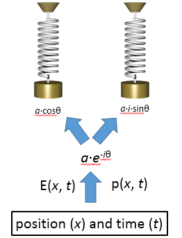
Intriguing title, isn’t it? You’ll think this is going to be highly speculative and you’re right. In fact, I could also have written: the imaginary action space, or the imaginary momentum space. Whatever. It all works ! It’s an imaginary space – but a very real one, because it holds energy, or momentum, or a combination of both, i.e. action. 🙂
So the title is either going to deter you or, else, encourage you to read on. I hope it’s the latter. 🙂
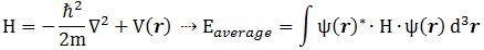
In my post on Richard Feynman’s exposé on how Schrödinger got his famous wave equation, I noted an ambiguity in how he deals with the energy concept. I wrote that piece in February, and we are now May. In-between, I looked at Schrödinger’s equation from various perspectives, as evidenced from the many posts that followed that February post, which I summarized on my Deep Blue page, where I note the following:
- The argument of the wavefunction (i.e. θ = ωt – kx = [E·t – p·x]/ħ) is just the proper time of the object that’s being represented by the wavefunction (which, in most cases, is an elementary particle—an electron, for example).
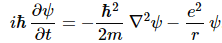
- The 1/2 factor in Schrödinger’s equation (∂ψ/∂t = i·(ħ/2m)·∇2ψ) doesn’t make all that much sense, so we should just drop it. Writing ∂ψ/∂t = i·(m/ħ)∇2ψ (i.e. Schrödinger’s equation without the 1/2 factor) does away with the mentioned ambiguities and, more importantly, avoids obvious contradictions.
Both remarks are rather unusual—especially the second one. In fact, if you’re not shocked by what I wrote above (Schrödinger got something wrong!), then stop reading—because then you’re likely not to understand a thing of what follows. 🙂 In any case, I thought it would be good to follow up by devoting a separate post to this matter.
The argument of the wavefunction as the proper time
Frankly, it took me quite a while to see that the argument of the wavefunction is nothing but the t’ = (t − v∙x)/√(1−v2)] formula that we know from the Lorentz transformation of spacetime. Let me quickly give you the formulas (just substitute the u for v):

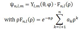
In fact, let me be precise: the argument of the wavefunction also has the particle’s rest mass m0 in it. That mass factor (m0) appears in it as a general scaling factor, so it determines the density of the wavefunction both in time as well as in space. Let me jot it down:
ψ(x, t) = a·e−i·(mv·t − p∙x) = a·e−i·[(m0/√(1−v2))·t − (m0·v/√(1−v2))∙x] = a·e−i·m0·(t − v∙x)/√(1−v2)
Huh? Yes. Let me show you how we get from θ = ωt – kx = [E·t – p·x]/ħ to θ = mv·t − p∙x. It’s really easy. We first need to choose our units such that the speed of light and Planck’s constant are numerically equal to one, so we write: c = 1 and ħ = 1. So now the 1/ħ factor no longer appears.
[Let me note something here: using natural units does not do away with the dimensions: the dimensions of whatever is there remain what they are. For example, energy remains what it is, and so that’s force over distance: 1 joule = 1 newton·meter (1 J = 1 N·m. Likewise, momentum remains what it is: force times time (or mass times velocity). Finally, the dimension of the quantum of action doesn’t disappear either: it remains the product of force, distance and time (N·m·s). So you should distinguish between the numerical value of our variables and their dimension. Always! That’s where physics is different from algebra: the equations actually mean something!]
Now, because we’re working in natural units, the numerical value of both c and c2 will be equal to 1. It’s obvious, then, that Einstein’s mass-energy equivalence relation reduces from E = mvc2 to E = mv. You can work out the rest yourself – noting that p = mv·v and mv = m0/√(1−v2). Done! For a more intuitive explanation, I refer you to the above-mentioned page.
So that’s for the wavefunction. Let’s now look at Schrödinger’s wave equation, i.e. that differential equation of which our wavefunction is a solution. In my introduction, I bluntly said there was something wrong with it: that 1/2 factor shouldn’t be there. Why not?
What’s wrong with Schrödinger’s equation?
When deriving his famous equation, Schrödinger uses the mass concept as it appears in the classical kinetic energy formula: K.E. = m·v2/2, and that’s why – after all the complicated turns – that 1/2 factor is there. There are many reasons why that factor doesn’t make sense. Let me sum up a few.
[I] The most important reason is that de Broglie made it quite clear that the energy concept in his equations for the temporal and spatial frequency for the wavefunction – i.e. the ω = E/ħ and k = p/ħ relations – is the total energy, including rest energy (m0), kinetic energy (m·v2/2) and any potential energy (V). In fact, if we just multiply the two de Broglie (aka as matter-wave equations) and use the old-fashioned v = f·λ relation (so we write E as E = ω·ħ = (2π·f)·(h/2π) = f·h, and p as p = k·ħ = (2π/λ)·(h/2π) = h/λ and, therefore, we have f = E/h and p = h/p), we find that the energy concept that’s implicit in the two matter-wave equations is equal to E = m∙v2, as shown below:
- f·λ = (E/h)·(h/p) = E/p
- v = f·λ ⇒ f·λ = v = E/p ⇔ E = v·p = v·(m·v) ⇒ E = m·v2
Huh? E = m∙v2? Yes. Not E = m∙c2 or m·v2/2 or whatever else you might be thinking of. In fact, this E = m∙v2 formula makes a lot of sense in light of the two following points.
Skeptical note: You may – and actually should – wonder whether we can use that v = f·λ relation for a wave like this, i.e. a wave with both a real (cos(-θ)) as well as an imaginary component (i·sin(-θ). It’s a deep question, and I’ll come back to it later. But… Yes. It’s the right question to ask. 😦
[II] Newton told us that force is mass time acceleration. Newton’s law is still valid in Einstein’s world. The only difference between Newton’s and Einstein’s world is that, since Einstein, we should treat the mass factor as a variable as well. We write: F = mv·a = mv·a = [m0/√(1−v2)]·a. This formula gives us the definition of the newton as a force unit: 1 N = 1 kg·(m/s)/s = 1 kg·m/s2. [Note that the 1/√(1−v2) factor – i.e. the Lorentz factor (γ) – has no dimension, because v is measured as a relative velocity here, i.e. as a fraction between 0 and 1.]
Now, you’ll agree the definition of energy as a force over some distance is valid in Einstein’s world as well. Hence, if 1 joule is 1 N·m, then 1 J is also equal to 1 (kg·m/s2)·m = 1 kg·(m2/s2), so this also reflects the E = m∙v2 concept. [I can hear you mutter: that kg factor refers to the rest mass, no? No. It doesn’t. The kg is just a measure of inertia: as a unit, it applies to both m0 as well as mv. Full stop.]
Very skeptical note: You will say this doesn’t prove anything – because this argument just shows the dimensional analysis for both equations (i.e. E = m∙v2 and E = m∙c2) is OK. Hmm… Yes. You’re right. 🙂 But the next point will surely convince you! 🙂
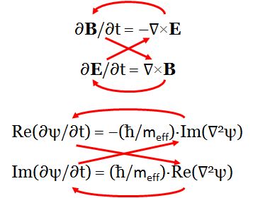
[III] The third argument is the most intricate and the most beautiful at the same time—not because it’s simple (like the arguments above) but because it gives us an interpretation of what’s going on here. It’s fairly easy to verify that Schrödinger’s equation, ∂ψ/∂t = i·(ħ/2m)·∇2ψ equation (including the 1/2 factor to which I object), is equivalent to the following set of two equations:
- Re(∂ψ/∂t) = −(ħ/2m)·Im(∇2ψ)
- Im(∂ψ/∂t) = (ħ/2m)·Re(∇2ψ)
[In case you don’t see it immediately, note that two complex numbers a + i·b and c + i·d are equal if, and only if, their real and imaginary parts are the same. However, here we have something like this: a + i·b = i·(c + i·d) = i·c + i2·d = − d + i·c (remember i2 = −1).]
Now, before we proceed (i.e. before I show you what’s wrong here with that 1/2 factor), let us look at the dimensions first. For that, we’d better analyze the complete Schrödinger equation so as to make sure we’re not doing anything stupid here by looking at one aspect of the equation only. The complete equation, in its original form, is:
Notice that, to simplify the analysis above, I had moved the i and the ħ on the left-hand side to the right-hand side (note that 1/i = −i, so −(ħ2/2m)/(i·ħ) = ħ/2m). Now, the ħ2 factor on the right-hand side is expressed in J2·s2. Now that doesn’t make much sense, but then that mass factor in the denominator makes everything come out alright. Indeed, we can use the mass-equivalence relation to express m in J/(m/s)2 units. So our ħ2/2m coefficient is expressed in (J2·s2)/[J/(m/s)2] = J·m2. Now we multiply that by that Laplacian operating on some scalar, which yields some quantity per square meter. So the whole right-hand side becomes some amount expressed in joule, i.e. the unit of energy! Interesting, isn’t it?
On the left-hand side, we have i and ħ. We shouldn’t worry about the imaginary unit because we can treat that as just another number, albeit a very special number (because its square is minus 1). However, in this equation, it’s like a mathematical constant and you can think of it as something like π or e. [Think of the magical formula: eiπ = i2 = −1.] In contrast, ħ is a physical constant, and so that constant comes with some dimension and, therefore, we cannot just do what we want. [I’ll show, later, that even moving it to the other side of the equation comes with interpretation problems, so be careful with physical constants, as they really mean something!] In this case, its dimension is the action dimension: J·s = N·m·s, so that’s force times distance times time. So we multiply that with a time derivative and we get joule once again (N·m·s/s = N·m = J), so that’s the unit of energy. So it works out: we have joule units both left and right in Schrödinger’s equation. Nice! Yes. But what does it mean? 🙂
Well… You know that we can – and should – think of Schrödinger’s equation as a diffusion equation – just like a heat diffusion equation, for example – but then one describing the diffusion of a probability amplitude. [In case you are not familiar with this interpretation, please do check my post on it, or my Deep Blue page.] But then we didn’t describe the mechanism in very much detail, so let me try to do that now and, in the process, finally explain the problem with the 1/2 factor.
The missing energy
There are various ways to explain the problem. One of them involves calculating group and phase velocities of the elementary wavefunction satisfying Schrödinger’s equation but that’s a more complicated approach and I’ve done that elsewhere, so just click the reference if you prefer the more complicated stuff. I find it easier to just use those two equations above:
- Re(∂ψ/∂t) = −(ħ/2m)·Im(∇2ψ)
- Im(∂ψ/∂t) = (ħ/2m)·Re(∇2ψ)
The argument is the following: if our elementary wavefunction is equal to ei(kx − ωt) = cos(kx−ωt) + i∙sin(kx−ωt), then it’s easy to proof that this pair of conditions is fulfilled if, and only if, ω = k2·(ħ/2m). [Note that I am omitting the normalization coefficient in front of the wavefunction: you can put it back in if you want. The argument here is valid, with or without normalization coefficients.] Easy? Yes. Check it out. The time derivative on the left-hand side is equal to:
∂ψ/∂t = −iω·iei(kx − ωt) = ω·[cos(kx − ωt) + i·sin(kx − ωt)] = ω·cos(kx − ωt) + iω·sin(kx − ωt)
And the second-order derivative on the right-hand side is equal to:
∇2ψ = ∂2ψ/∂x2 = i·k2·ei(kx − ωt) = k2·cos(kx − ωt) + i·k2·sin(kx − ωt)
So the two equations above are equivalent to writing:
- Re(∂ψB/∂t) = −(ħ/2m)·Im(∇2ψB) ⇔ ω·cos(kx − ωt) = k2·(ħ/2m)·cos(kx − ωt)
- Im(∂ψB/∂t) = (ħ/2m)·Re(∇2ψB) ⇔ ω·sin(kx − ωt) = k2·(ħ/2m)·sin(kx − ωt)
So both conditions are fulfilled if, and only if, ω = k2·(ħ/2m). You’ll say: so what? Well… We have a contradiction here—something that doesn’t make sense. Indeed, the second of the two de Broglie equations (always look at them as a pair) tells us that k = p/ħ, so we can re-write the ω = k2·(ħ/2m) condition as:
ω/k = vp = k2·(ħ/2m)/k = k·ħ/(2m) = (p/ħ)·(ħ/2m) = p/2m ⇔ p = 2m
You’ll say: so what? Well… Stop reading, I’d say. That p = 2m doesn’t make sense—at all! Nope! In fact, if you thought that the E = m·v2 is weird—which, I hope, is no longer the case by now—then… Well… This p = 2m equation is much weirder. In fact, it’s plain nonsense: this condition makes no sense whatsoever. The only way out is to remove the 1/2 factor, and to re-write the Schrödinger equation as I wrote it, i.e. with an ħ/m coefficient only, rather than an (1/2)·(ħ/m) coefficient.
Huh? Yes.
As mentioned above, I could do those group and phase velocity calculations to show you what rubbish that 1/2 factor leads to – and I’ll do that eventually – but let me first find yet another way to present the same paradox. Let’s simplify our life by choosing our units such that c = ħ = 1, so we’re using so-called natural units rather than our SI units. [Again, note that switching to natural units doesn’t do anything to the physical dimensions: a force remains a force, a distance remains a distance, and so on.] Our mass-energy equivalence then becomes: E = m·c2 = m·12 = m. [Again, note that switching to natural units doesn’t do anything to the physical dimensions: a force remains a force, a distance remains a distance, and so on. So we’d still measure energy and mass in different but equivalent units. Hence, the equality sign should not make you think mass and energy are actually the same: energy is energy (i.e. force times distance), while mass is mass (i.e. a measure of inertia). I am saying this because it’s important, and because it took me a while to make these rather subtle distinctions.]
Let’s now go one step further and imagine a hypothetical particle with zero rest mass, so m0 = 0. Hence, all its energy is kinetic and so we write: K.E. = mv·v/2. Now, because this particle has zero rest mass, the slightest acceleration will make it travel at the speed of light. In fact, we would expect it to travel at the speed, so mv = mc and, according to the mass-energy equivalence relation, its total energy is, effectively, E = mv = mc. However, we just said its total energy is kinetic energy only. Hence, its total energy must be equal to E = K.E. = mc·c/2 = mc/2. So we’ve got only half the energy we need. Where’s the other half? Where’s the missing energy? Quid est veritas? Is its energy E = mc or E = mc/2?
It’s just a paradox, of course, but one we have to solve. Of course, we may just say we trust Einstein’s E = m·c2 formula more than the kinetic energy formula, but that answer is not very scientific. 🙂 We’ve got a problem here and, in order to solve it, I’ve come to the following conclusion: just because of its sheer existence, our zero-mass particle must have some hidden energy, and that hidden energy is also equal to E = m·c2/2. Hence, the kinetic and the hidden energy add up to E = m·c2 and all is alright.
Huh? Hidden energy? I must be joking, right?
Well… No. Let me explain. Oh. And just in case you wonder why I bother to try to imagine zero-mass particles. Let me tell you: it’s the first step towards finding a wavefunction for a photon and, secondly, you’ll see it just amounts to modeling the propagation mechanism of energy itself. 🙂
The hidden energy as imaginary energy
I am tempted to refer to the missing energy as imaginary energy, because it’s linked to the imaginary part of the wavefunction. However, it’s anything but imaginary: it’s as real as the imaginary part of the wavefunction. [I know that sounds a bit nonsensical, but… Well… Think about it. And read on!]
Back to that factor 1/2. As mentioned above, it also pops up when calculating the group and the phase velocity of the wavefunction. In fact, let me show you that calculation now. [Sorry. Just hang in there.] It goes like this.
The de Broglie relations tell us that the k and the ω in the ei(kx − ωt) = cos(kx−ωt) + i∙sin(kx−ωt) wavefunction (i.e. the spatial and temporal frequency respectively) are equal to k = p/ħ, and ω = E/ħ. Let’s now think of that zero-mass particle once more, so we assume all of its energy is kinetic: no rest energy, no potential! So… If we now use the kinetic energy formula E = m·v2/2 – which we can also write as E = m·v·v/2 = p·v/2 = p·p/2m = p2/2m, with v = p/m the classical velocity of the elementary particle that Louis de Broglie was thinking of – then we can calculate the group velocity of our ei(kx − ωt) = cos(kx−ωt) + i∙sin(kx−ωt) wavefunction as:
vg = ∂ω/∂k = ∂[E/ħ]/∂[p/ħ] = ∂E/∂p = ∂[p2/2m]/∂p = 2p/2m = p/m = v
[Don’t tell me I can’t treat m as a constant when calculating ∂ω/∂k: I can. Think about it.]
Fine. Now the phase velocity. For the phase velocity of our ei(kx − ωt) wavefunction, we find:
vp = ω/k = (E/ħ)/(p/ħ) = E/p = (p2/2m)/p = p/2m = v/2
So that’s only half of v: it’s the 1/2 factor once more! Strange, isn’t it? Why would we get a different value for the phase velocity here? It’s not like we have two different frequencies here, do we? Well… No. You may also note that the phase velocity turns out to be smaller than the group velocity (as mentioned, it’s only half of the group velocity), which is quite exceptional as well! So… Well… What’s the matter here? We’ve got a problem!
What’s going on here? We have only one wave here—one frequency and, hence, only one k and ω. However, on the other hand, it’s also true that the ei(kx − ωt) wavefunction gives us two functions for the price of one—one real and one imaginary: ei(kx − ωt) = cos(kx−ωt) + i∙sin(kx−ωt). So the question here is: are we adding waves, or are we not? It’s a deep question. If we’re adding waves, we may get different group and phase velocities, but if we’re not, then… Well… Then the group and phase velocity of our wave should be the same, right? The answer is: we are and we aren’t. It all depends on what you mean by ‘adding’ waves. I know you don’t like that answer, but that’s the way it is, really. 🙂
Let me make a small digression here that will make you feel even more confused. You know – or you should know – that the sine and the cosine function are the same except for a phase difference of 90 degrees: sinθ = cos(θ + π/2). Now, at the same time, multiplying something with i amounts to a rotation by 90 degrees, as shown below.
Hence, in order to sort of visualize what our ei(kx − ωt) function really looks like, we may want to super-impose the two graphs and think of something like this:
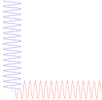
You’ll have to admit that, when you see this, our formulas for the group or phase velocity, or our v = f·λ relation, do no longer make much sense, do they? 🙂
Having said that, that 1/2 factor is and remains puzzling, and there must be some logical reason for it. For example, it also pops up in the Uncertainty Relations:
Δx·Δp ≥ ħ/2 and ΔE·Δt ≥ ħ/2
So we have ħ/2 in both, not ħ. Why do we need to divide the quantum of action here? How do we solve all these paradoxes? It’s easy to see how: the apparent contradiction (i.e. the different group and phase velocity) gets solved if we’d use the E = m∙v2 formula rather than the kinetic energy E = m∙v2/2. But then… What energy formula is the correct one: E = m∙v2 or m∙c2? Einstein’s formula is always right, isn’t it? It must be, so let me postpone the discussion a bit by looking at a limit situation. If v = c, then we don’t need to make a choice, obviously. 🙂 So let’s look at that limit situation first. So we’re discussing our zero-mass particle once again, assuming it travels at the speed of light. What do we get?
Well… Measuring time and distance in natural units, so c = 1, we have:
E = m∙c2 = m and p = m∙c = m, so we get: E = m = p
Waw ! E = m = p ! What a weird combination, isn’t it? Well… Yes. But it’s fully OK. [You tell me why it wouldn’t be OK. It’s true we’re glossing over the dimensions here, but natural units are natural units and, hence, the numerical value of c and c2 is 1. Just figure it out for yourself.] The point to note is that the E = m = p equality yields extremely simple but also very sensible results. For the group velocity of our ei(kx − ωt) wavefunction, we get:
vg = ∂ω/∂k = ∂[E/ħ]/∂[p/ħ] = ∂E/∂p = ∂p/∂p = 1
So that’s the velocity of our zero-mass particle (remember: the 1 stands for c here, i.e. the speed of light) expressed in natural units once more—just like what we found before. For the phase velocity, we get:
vp = ω/k = (E/ħ)/(p/ħ) = E/p = p/p = 1
Same result! No factor 1/2 here! Isn’t that great? My ‘hidden energy theory’ makes a lot of sense.
However, if there’s hidden energy, we still need to show where it’s hidden. 🙂 Now that question is linked to the propagation mechanism that’s described by those two equations, which now – leaving the 1/2 factor out, simplify to:
- Re(∂ψ/∂t) = −(ħ/m)·Im(∇2ψ)
- Im(∂ψ/∂t) = (ħ/m)·Re(∇2ψ)
Propagation mechanism? Yes. That’s what we’re talking about here: the propagation mechanism of energy. Huh? Yes. Let me explain in another separate section, so as to improve readability. Before I do, however, let me add another note—for the skeptics among you. 🙂
Indeed, the skeptics among you may wonder whether our zero-mass particle wavefunction makes any sense at all, and they should do so for the following reason: if x = 0 at t = 0, and it’s traveling at the speed of light, then x(t) = t. Always. So if E = m = p, the argument of our wavefunction becomes E·t – p·x = E·t – E·t = 0! So what’s that? The proper time of our zero-mass particle is zero—always and everywhere!?
Well… Yes. That’s why our zero-mass particle – as a point-like object – does not really exist. What we’re talking about is energy itself, and its propagation mechanism. 🙂
While I am sure that, by now, you’re very tired of my rambling, I beg you to read on. Frankly, if you got as far as you have, then you should really be able to work yourself through the rest of this post. 🙂 And I am sure that – if anything – you’ll find it stimulating! 🙂
The imaginary energy space
Look at the propagation mechanism for the electromagnetic wave in free space, which (for c = 1) is represented by the following two equations:
- ∂B/∂t = –∇×E
- ∂E/∂t = ∇×B
[In case you wonder, these are Maxwell’s equations for free space, so we have no stationary nor moving charges around.] See how similar this is to the two equations above? In fact, in my Deep Blue page, I use these two equations to derive the quantum-mechanical wavefunction for the photon (which is not the same as that hypothetical zero-mass particle I introduced above), but I won’t bother you with that here. Just note the so-called curl operator in the two equations above (∇×) can be related to the Laplacian we’ve used so far (∇2). It’s not the same thing, though: for starters, the curl operator operates on a vector quantity, while the Laplacian operates on a scalar (including complex scalars). But don’t get distracted now. Let’s look at the revised Schrödinger’s equation, i.e. the one without the 1/2 factor:
∂ψ/∂t = i·(ħ/m)·∇2ψ
On the left-hand side, we have a time derivative, so that’s a flow per second. On the right-hand side we have the Laplacian and the i·ħ/m factor. Now, written like this, Schrödinger’s equation really looks exactly the same as the general diffusion equation, which is written as: ∂φ/∂t = D·∇2φ, except for the imaginary unit, which makes it clear we’re getting two equations for the price of one here, rather than one only! 🙂 The point is: we may now look at that ħ/m factor as a diffusion constant, because it does exactly the same thing as the diffusion constant D in the diffusion equation ∂φ/∂t = D·∇2φ, i.e:
- As a constant of proportionality, it quantifies the relationship between both derivatives.
- As a physical constant, it ensures the dimensions on both sides of the equation are compatible.
So the diffusion constant for Schrödinger’s equation is ħ/m. What is its dimension? That’s easy: (N·m·s)/(N·s2/m) = m2/s. [Remember: 1 N = 1 kg·m/s2.] But then we multiply it with the Laplacian, so that’s something expressed per square meter, so we get something per second on both sides.
Of course, you wonder: what per second? Not sure. That’s hard to say. Let’s continue with our analogy with the heat diffusion equation so as to try to get a better understanding of what’s being written here. Let me give you that heat diffusion equation here. Assuming the heat per unit volume (q) is proportional to the temperature (T) – which is the case when expressing T in degrees Kelvin (K), so we can write q as q = k·T – we can write it as:

So that’s structurally similar to Schrödinger’s equation, and to the two equivalent equations we jotted down above. So we’ve got T (temperature) in the role of ψ here—or, to be precise, in the role of ψ ‘s real and imaginary part respectively. So what’s temperature? From the kinetic theory of gases, we know that temperature is not just a scalar: temperature measures the mean (kinetic) energy of the molecules in the gas. That’s why we can confidently state that the heat diffusion equation models an energy flow, both in space as well as in time.
Let me make the point by doing the dimensional analysis for that heat diffusion equation. The time derivative on the left-hand side (∂T/∂t) is expressed in K/s (Kelvin per second). Weird, isn’t it? What’s a Kelvin per second? Well… Think of a Kelvin as some very small amount of energy in some equally small amount of space—think of the space that one molecule needs, and its (mean) energy—and then it all makes sense, doesn’t it?
However, in case you find that a bit difficult, just work out the dimensions of all the other constants and variables. The constant in front (k) makes sense of it. That coefficient (k) is the (volume) heat capacity of the substance, which is expressed in J/(m3·K). So the dimension of the whole thing on the left-hand side (k·∂T/∂t) is J/(m3·s), so that’s energy (J) per cubic meter (m3) and per second (s). Nice, isn’t it? What about the right-hand side? On the right-hand side we have the Laplacian operator – i.e. ∇2 = ∇·∇, with ∇ = (∂/∂x, ∂/∂y, ∂/∂z) – operating on T. The Laplacian operator, when operating on a scalar quantity, gives us a flux density, i.e. something expressed per square meter (1/m2). In this case, it’s operating on T, so the dimension of ∇2T is K/m2. Again, that doesn’t tell us very much (what’s the meaning of a Kelvin per square meter?) but we multiply it by the thermal conductivity (κ), whose dimension is W/(m·K) = J/(m·s·K). Hence, the dimension of the product is the same as the left-hand side: J/(m3·s). So that’s OK again, as energy (J) per cubic meter (m3) and per second (s) is definitely something we can associate with an energy flow.
In fact, we can play with this. We can bring k from the left- to the right-hand side of the equation, for example. The dimension of κ/k is m2/s (check it!), and multiplying that by K/m2 (i.e. the dimension of ∇2T) gives us some quantity expressed in Kelvin per second, and so that’s the same dimension as that of ∂T/∂t. Done!
In fact, we’ve got two different ways of writing Schrödinger’s diffusion equation. We can write it as ∂ψ/∂t = i·(ħ/m)·∇2ψ or, else, we can write it as ħ·∂ψ/∂t = i·(ħ2/m)·∇2ψ. Does it matter? I don’t think it does. The dimensions come out OK in both cases. However, interestingly, if we do a dimensional analysis of the ħ·∂ψ/∂t = i·(ħ2/m)·∇2ψ equation, we get joule on both sides. Interesting, isn’t it? The key question, of course, is: what is it that is flowing here?
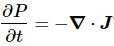
I don’t have a very convincing answer to that, but the answer I have is interesting—I think. 🙂 Think of the following: we can multiply Schrödinger’s equation with whatever we want, and then we get all kinds of flows. For example, if we multiply both sides with 1/(m2·s) or 1/(m3·s), we get a equation expressing the energy conservation law, indeed! [And you may want to think about the minus sign of the right-hand side of Schrödinger’s equation now, because it makes much more sense now!]
We could also multiply both sides with s, so then we get J·s on both sides, i.e. the dimension of physical action (J·s = N·m·s). So then the equation expresses the conservation of action! Huh? Yes. Let me re-phrase that: then it expresses the conservation of angular momentum—as you’ll surely remember that the dimension of action and angular momentum are the same. 🙂
And then we can divide both sides by m, so then we get N·s on both sides, so that’s momentum. So then Schrödinger’s equation embodies the momentum conservation law.
Isn’t it just wonderful? Schrödinger’s equation packs all of the conservation laws! The only catch is that it flows back and forth from the real to the imaginary space, using that propagation mechanism as described in those two equations.
Now that is really interesting, because it does provide an explanation – as fuzzy as it may seem – for all those weird concepts one encounters when studying physics, such as the tunneling effect, which amounts to energy flowing from the imaginary space to the real space and, then, inevitably, flowing back. It also allows for borrowing time from the imaginary space. Hmm… Interesting! [I know I still need to make these points much more formally, but… Well… You kinda get what I mean, don’t you?]
To conclude, let me re-baptize my real and imaginary ‘space’ by referring to them to what they really are: a real and imaginary energy space respectively. Although… Now that I think of it: it could also be real and imaginary momentum space, or a real and imaginary action space. Hmm… The latter term may be the best. 🙂
Isn’t this all great? I mean… I could go on and on—but I’ll stop here, so you can freewheel around yourself. For example, you may wonder how similar that energy propagation mechanism actually is as compared to the propagation mechanism of the electromagnetic wave? The answer is: very similar. You can check how similar in one of my posts on the photon wavefunction or, if you’d want a more general argument, check my Deep Blue page. Have fun exploring! 🙂
So… Well… That’s it, folks. I hope you enjoyed this post—if only because I really enjoyed writing it. 🙂
[…]
OK. You’re right. I still haven’t answered the fundamental question.
So what about the 1/2 factor?
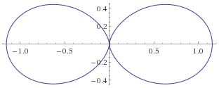
What about that 1/2 factor? Did Schrödinger miss it? Well… Think about it for yourself. First, I’d encourage you to further explore that weird graph with the real and imaginary part of the wavefunction. I copied it below, but with an added 45º line—yes, the green diagonal. To make it somewhat more real, imagine you’re the zero-mass point-like particle moving along that line, and we observe you from our inertial frame of reference, using equivalent time and distance units.
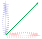
So we’ve got that cosine (cosθ) varying as you travel, and we’ve also got the i·sinθ part of the wavefunction going while you’re zipping through spacetime. Now, THINK of it: the phase velocity of the cosine bit (i.e. the red graph) contributes as much to your lightning speed as the i·sinθ bit, doesn’t it? Should we apply Pythagoras’ basic r2 = x2 + y2 Theorem here? Yes: the velocity vector along the green diagonal is going to be the sum of the velocity vectors along the horizontal and vertical axes. So… That’s great.
Yes. It is. However, we still have a problem here: it’s the velocity vectors that add up—not their magnitudes. Indeed, if we denote the velocity vector along the green diagonal as u, then we can calculate its magnitude as:
u = √u2 = √[(v/2)2 + (v/2)2] = √[2·(v2/4) = √[v2/2] = v/√2 ≈ 0.7·v
So, as mentioned, we’re adding the vectors, but not their magnitudes. We’re somewhat better off than we were in terms of showing that the phase velocity of those sine and cosine velocities add up—somehow, that is—but… Well… We’re not quite there.
Fortunately, Einstein saves us once again. Remember we’re actually transforming our reference frame when working with the wavefunction? Well… Look at the diagram below (for which I thank the author)
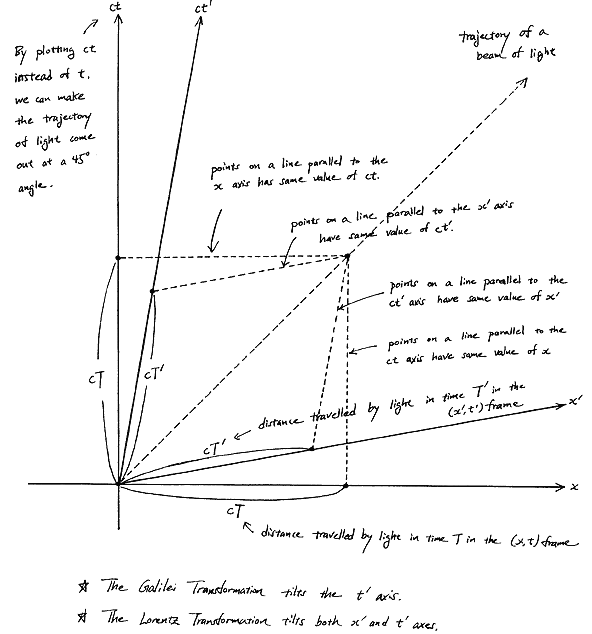
In fact, let me insert an animated illustration, which shows what happens when the velocity u goes up and down from (close to) −c to +c and back again. It’s beautiful, and I must credit the author here too. It sort of speaks for itself, but please do click the link as the accompanying text is quite illuminating. 🙂
The point is: for our zero-mass particle, the x’ and t’ axis will rotate into the diagonal itself which, as I mentioned a couple of times already, represents the speed of light and, therefore, our zero-mass particle traveling at c. It’s obvious that we’re now adding two vectors that point in the same direction and, hence, their magnitudes just add without any square root factor. So, instead of u = √[(v/2)2 + (v/2)2], we just have v/2 + v/2 = v! Done! We solved the phase velocity paradox! 🙂
So… I still haven’t answered that question. Should that 1/2 factor in Schrödinger’s equation be there or not? The answer is, obviously: yes. It should be there. And as for Schrödinger using the mass concept as it appears in the classical kinetic energy formula: K.E. = m·v2/2… Well… What other mass concept would he use? I probably got a bit confused with Feynman’s exposé – especially this notion of ‘choosing the zero point for the energy’ – but then I should probably just re-visit the thing and adjust the language here and there. But the formula is correct.
Thinking it all through, the ħ/2m constant in Schrödinger’s equation should be thought of as the reciprocal of m/(ħ/2). So what we’re doing basically is measuring the mass of our object in units of ħ/2, rather than units of ħ. That makes perfect sense, if only because it’s ħ/2, rather than ħthe factor that appears in the Uncertainty Relations Δx·Δp ≥ ħ/2 and ΔE·Δt ≥ ħ/2. In fact, in my post on the wavefunction of the zero-mass particle, I noted its elementary wavefunction should use the m = E = p = ħ/2 values, so it becomes ψ(x, t) = a·e−i∙[(ħ/2)∙t − (ħ/2)∙x]/ħ = a·e−i∙[t − x]/2.
Isn’t that just nice? 🙂 I need to stop here, however, because it looks like this post is becoming a book. Oh—and note that nothing what I wrote above discredits my ‘hidden energy’ theory. On the contrary, it confirms it. In fact, the nice thing about those illustrations above is that it associates the imaginary component of our wavefunction with travel in time, while the real component is associated with travel in space. That makes our theory quite complete: the ‘hidden’ energy is the energy that moves time forward. The only thing I need to do is to connect it to that idea of action expressing itself in time or in space, cf. what I wrote on my Deep Blue page: we can look at the dimension of Planck’s constant, or at the concept of action in general, in two very different ways—from two different perspectives, so to speak:
- [Planck’s constant] = [action] = N∙m∙s = (N∙m)∙s = [energy]∙[time]
- [Planck’s constant] = [action] = N∙m∙s = (N∙s)∙m = [momentum]∙[distance]
Hmm… I need to combine that with the idea of the quantum vacuum, i.e. the mathematical space that’s associated with time and distance becoming countable variables…. In any case. Next time. 🙂
Before I sign off, however, let’s quickly check if our a·e−i∙[t − x]/2 wavefunction solves the Schrödinger equation:
- ∂ψ/∂t = −a·e−i∙[t − x]/2·(i/2)
- ∇2ψ = ∂2[a·e−i∙[t − x]/2]/∂x2 = ∂[a·e−i∙[t − x]/2·(i/2)]/∂x = −a·e−i∙[t − x]/2·(1/4)
So the ∂ψ/∂t = i·(ħ/2m)·∇2ψ equation becomes:
−a·e−i∙[t − x]/2·(i/2) = −i·(ħ/[2·(ħ/2)])·a·e−i∙[t − x]/2·(1/4)
⇔ 1/2 = 1/4 !?
The damn 1/2 factor. Schrödinger wants it in his wave equation, but not in the wavefunction—apparently! So what if we take the m = E = p = ħ solution? We get:
- ∂ψ/∂t = −a·i·e−i∙[t − x]
- ∇2ψ = ∂2[a·e−i∙[t − x]]/∂x2 = ∂[a·i·e−i∙[t − x]]/∂x = −a·e−i∙[t − x]
So the ∂ψ/∂t = i·(ħ/2m)·∇2ψ equation now becomes:
−a·i·e−i∙[t − x] = −i·(ħ/[2·ħ])·a·e−i∙[t − x]
⇔ 1 = 1/2 !?
We’re still in trouble! So… Was Schrödinger wrong after all? There’s no difficulty whatsoever with the ∂ψ/∂t = i·(ħ/m)·∇2ψ equation:
- −a·e−i∙[t − x]/2·(i/2) = −i·[ħ/(ħ/2)]·a·e−i∙[t − x]/2·(1/4) ⇔ 1 = 1
- −a·i·e−i∙[t − x] = −i·(ħ/ħ)·a·e−i∙[t − x] ⇔ 1 = 1
What these equations might tell us is that we should measure mass, energy and momentum in terms of ħ (and not in terms of ħ/2) but that the fundamental uncertainty is ± ħ/2. That solves it all. So the magnitude of the uncertainty is ħ but it separates not 0 and ± 1, but −ħ/2 and −ħ/2. Or, more generally, the following series:
…, −7ħ/2, −5ħ/2, −3ħ/2, −ħ/2, +ħ/2, +3ħ/2,+5ħ/2, +7ħ/2,…
Why are we not surprised? The series represent the energy values that a spin one-half particle can possibly have, and ordinary matter – i.e. all fermions – is composed of spin one-half particles.
To conclude this post, let’s see if we can get any indication on the energy concepts that Schrödinger’s revised wave equation implies. We’ll do so by just calculating the derivatives in the ∂ψ/∂t = i·(ħ/m)·∇2ψ equation (i.e. the equation without the 1/2 factor). Let’s also not assume we’re measuring stuff in natural units, so our wavefunction is just what it is: a·e−i·[E·t − p∙x]/ħ. The derivatives now become:
- ∂ψ/∂t = −a·i·(E/ħ)·e−i∙[E·t − p∙x]/ħ
- ∇2ψ = ∂2[a·e−i∙[E·t − p∙x]/ħ]/∂x2 = ∂[a·i·(p/ħ)·e−i∙[E·t − p∙x]/ħ]/∂x = −a·(p2/ħ2)·e−i∙[E·t − p∙x]/ħ
So the ∂ψ/∂t = i·(ħ/m)·∇2ψ = i·(1/m)·∇2ψ equation now becomes:
−a·i·(E/ħ)·e−i∙[E·t − p∙x]/ħ = −i·(ħ/m)·a·(p2/ħ2)·e−i∙[E·t − p∙x]/ħ ⇔ E = p2/m = m·v2
It all works like a charm. Note that we do not assume stuff like E = m = p here. It’s all quite general. Also note that the E = p2/m closely resembles the kinetic energy formula one often sees: K.E. = m·v2/2 = m·m·v2/(2m) = p2/(2m). We just don’t have the 1/2 factor in our E = p2/m formula, which is great—because we don’t want it! Of course, if you’d add the 1/2 factor in Schrödinger’s equation again, you’d get it back in your energy formula, which would just be that old kinetic energy formula which gave us all these contradictions and ambiguities. 😦
Finally, and just to make sure: let me add that, when we wrote that E = m = p – like we did above – we mean their numerical values are the same. Their dimensions remain what they are, of course. Just to make sure you get that subtle point, we’ll do a quick dimensional analysis of that E = p2/m formula:
[E] = [p2/m] ⇔ N·m = N2·s2/kg = N2·s2/[N·m/s2] = N·m = joule (J)
So… Well… It’s all perfect. 🙂
Post scriptum: I revised my Deep Blue page after writing this post, and I think that a number of the ideas that I express above are presented more consistently and coherently there. In any case, the missing energy theory makes sense. Think of it: any oscillator involves both kinetic as well as potential energy, and they both add up to twice the average kinetic (or potential) energy. So why not here? When everything is said and done, our elementary wavefunction does describe an oscillator. 🙂
Some content on this page was disabled on June 16, 2020 as a result of a DMCA takedown notice from The California Institute of Technology. You can learn more about the DMCA here:
https://wordpress.com/support/copyright-and-the-dmca/

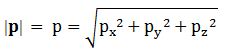
 The J·J in the classical formula above is, of course, the equally classical vector dot product, and the formula itself is nothing but Pythagoras’ Theorem in three dimensions. Easy. I just put a + sign in front of the square roots so as to remind you we actually always have two square roots and that we should take the positive one. 🙂
 So now we can apply our classical J·J = Jx2 + Jy2 + Jz2 formula to these quantities by calculating the expected value of J = J·J, which is equal to:
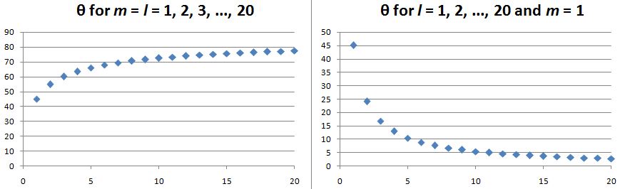
 But… Well… Note those weird angles: we get something close to 24.1° and then another value close to 54.7°. No symmetry here. 😦 The table below gives some more values for larger j. They’re easy to calculate – it’s, once again, just Pythagoras’ Theorem – but… Well… No symmetries here. Just weird values. [I am not saying the formula for these angles is not straightforward. That formula is easy enough: θ = sin-1(m/√[j(j+1)]). It’s just… Well… No symmetry. You’ll see why that matters in a moment.]
 I skipped the half-integer values for j in the table above so you might think they might make it easier to come up with some kind of sensible explanation for the angles. Well… No. They don’t. For example, for j = 1/2 and m = ± 1/2, the angles are ±35.2644° – more or less, that is. 🙂 As you can see, these angles do not nicely cut up our circle in equal pieces, which triggers the obvious question: are these angles really equally likely? Equal angles do not correspond to equal distances on the z-axis (in case you don’t appreciate the point, look at the illustration below).
 That’s why physicists tell us that, in quantum mechanics, the angular momentum is never “completely along the z-direction.” It is obvious that this actually challenges the idea of a very precise direction in quantum mechanics, but then that shouldn’t surprise us, does it? After, isn’t this what the Uncertainty Principle is all about?
 The nutation is caused by the gravitational force field, and the nutation movement usually dies out quickly because of dampening forces (read: friction). Now, we don’t think of gravitational fields when analyzing angular momentum in quantum mechanics, and we shouldn’t. But there is something else we may want to think of. There is also a phenomenon which is referred to as free nutation, i.e. a nutation that is not caused by an external force field. The Earth, for example, nutates slowly because of a gravitational pull from the Sun and the other planets – so that’s not a free nutation – but, in addition to this, there’s an even smaller wobble – which is an example of free nutation – because the Earth is not exactly spherical. In fact, the Great Mathematician, Leonhard Euler, had already predicted this, back in 1765, but it took another 125 years or so before an astronomist, Seth Chandler, could finally experimentally confirm and measure it. So they named this wobble the Chandler wobble (Euler already has too many things named after him). 🙂
 I am not sure if this approach would solve the problem of our angles and distances – the issue of whether we should think in equally likely angles or equally likely distances along the z-axis, really – but… Well… I’ll let you play with this. Please do send me some feedback if you think you’ve found something. 🙂
 In fact, now that I’ve shown this graph, I should quickly explain it. The three graphs are the spherically symmetric wavefunctions for the first three energy levels. For the first energy level – which is conventionally written as n = 1, not as n = 0 – the amplitude approaches zero rather quickly. For n = 2 and n = 3, there are zero-crossings: the curve passes the r-axis. Feynman calls these zero-crossing radial nodes. To be precise, the number of zero-crossings for these s-states is n − 1, so there’s none for n = 1, one for n = 2, two for n = 3, etcetera.
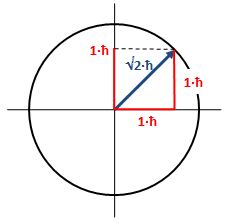 What if l = 2? The magnitude of l is then equal to √[2·(2+1)]·ħ = √6·ħ ≈ 2.4495·ħ. How do we relate that to those “cocked” angles? The values of m now range from -2 to +2, with a unit distance in-between. The illustration below shows the angles. [I didn’t mention ħ any more in that illustration because, by now, we should know it’s our unit of measurement – always.]
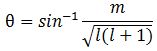 It’s simple but intriguing. Needless to say, the sin −1 function is the inverse sine, also known as the arcsine. I’ve calculated the values for all m for l = 1, 2, 3, 4 and 5 below. The most interesting values are the angles for m = 1 and m = l. As the graphs underneath show, for m = 1, the values start approaching the zero angle for very large l, so there’s not much difference any more between m = ±1 and m = 1 for large values of l. What about the m = l case? Well… Believe it or not, if l becomes really large, then these angles do approach 90°. If you don’t remember how to calculate limits, then just calculate θ for some huge value for l and m. For l = m = 1,000,000, for example, you should find that θ = 89.9427…°. 🙂
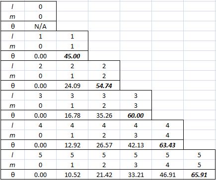
 Isn’t this fascinating? I’ve actually never seen this in a textbook – so it might be an original contribution. 🙂 OK. I need to get back to the grind:
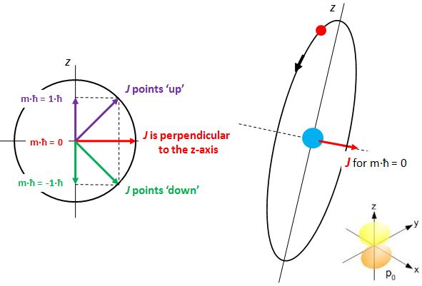

 A more complete table is given below:
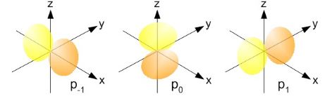
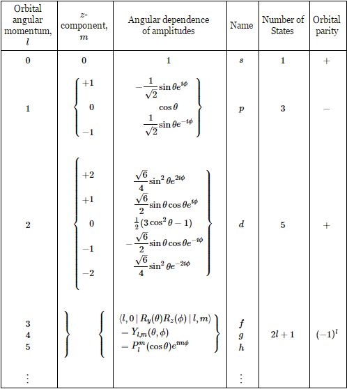 So, yes, we’re done. Those equations above give us those wonderful shapes for the electron orbitals, as illustrated below (credit for the illustration goes to
 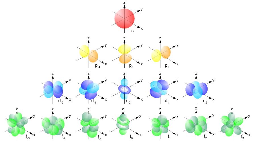 But… Hey! Wait a moment! We only have these Yl,m(θ, φ) functions here. What about Fl(r)?
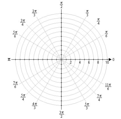
 So far, so good. But what happens if we have two polarizers, set up as shown below, with the optical axis of the first one at an angle θ, which is, say, equal to 30°? Will any light get through?
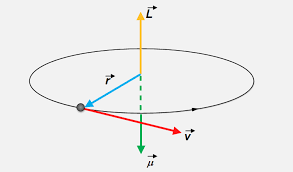 So the electron orbit – in whatever way we’d want to visualize it – gives us L, which we refer to as the orbital angular momentum. We know the electron is also supposed to spin about its own axis – even if we know this planetary model of an electron isn’t quite correct. So that gives us a spin angular momentum S. In the so-called
  If J is the sum of two other vectors L and S, then this has rather weird implications for the precession of L and S, as shown in the illustration below – which I took from the
  More importantly, our classical model also gets into trouble when actually measuring the magnitude of Jz: repeated measurements will not yield some randomly distributed continuous variable, as one would classically expect. No. In fact, that’s what this experiment is all about: it shows that Jz will take only certain quantized values. That is what is shown in the illustration below (which once again assumes the magnetic field (B) is along the z-axis).
 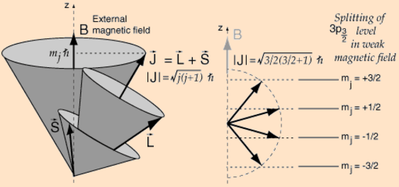 I copied the illustration above from
  Hmm… What about those illustrations on the right-hand side – with the vector sums and those values for j and mj? I guess the idea may also be illustrated by the table below: combining different values for l (±1) and s (±1/2) gives four possible values, ranging from +3/2 to -1/2, for j = l + s.
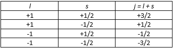 Having said that, the illustration raises a very fundamental question: the length of the sum of two vectors is definitely not the same as the sum of the length of the two vectors! So… Well… Hmm… Something doesn’t make sense here! However, I can’t dwell any longer on this. I just wanted to note you should not take all that’s published on those oft-used sites on quantum mechanics for granted. But so I need to move on. Back to the other illustration – copied once more below.
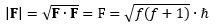
 In case you’d want to check this, you can check
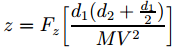
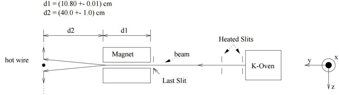
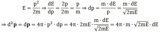
 The next step is to use this formula so as to be able to calculate a distribution which would describe the intensity of the beam. Now, it’s easy to understand such intensity will be related to the flux of potassium atoms, and it’s equally easy to get that a flux is defined as the rate of flow per unit area. Hmm… So how does this get us the formula below?
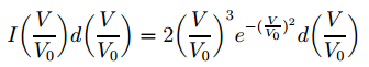 The tricky thing – of course – is the use of those normalized velocities because… Well… It’s easy to see that the right-hand side of the equation above – just forget about the d(V/V0 ) bit for a second, as we have it on both sides of the equation and so it cancels out anyway – is just density times velocity. We do have a product of the density of particles and the velocity with which they emerge here – albeit a normalized velocity. But then… Who cares? The normalization is just a division by V0 – or a multiplication by 1/V0, which is some constant. From a math point of view, it doesn’t make any difference: our variable is V/V0 instead of V. It’s just like using some other unit. No worries here – as long as you use the new variable consistently everywhere. 🙂
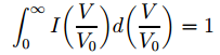 So… What’s next… Well… We’re almost there. 🙂 As the MIT paper notes, the f(V) and I(V/V0) functions can be mapped to each other: the related transformation maps a velocity distribution to an intensity distribution – i.e. a distribution of the deflection – and vice versa.
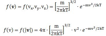
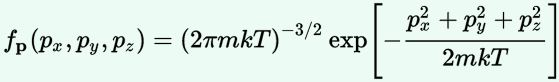
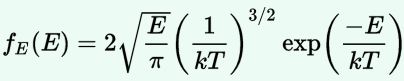
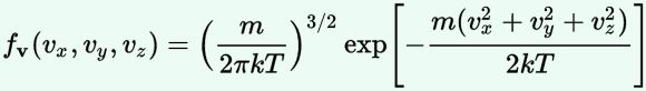
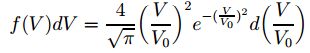
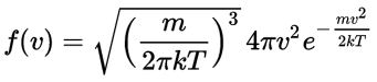 Now, the final thing to note is that you’ll often want to use so-called normalized velocities, i.e. velocities that are defined as a v/v0 ratio, with v0 the most probable speed, which is equal to √(2kT/m). You get that value by calculating the df(v)/dv derivative, and then finding the value v = v0 for which df(v)/dv = 0. You should now be able to verify the formula that is used in the mentioned MIT version of the Stern-Gerlach experiment:
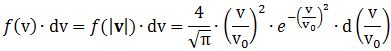 Indeed, when you write it all out – note that π/π3/2 = 1/√π 🙂 – you’ll see the two formulas are effectively equivalent. Of course, by now you are completely formula-ed out, and so you probably don’t even wonder what that f(v)·dv product actually stands for. What does it mean, really? Now you’ll sigh: why would I even want to know that? Well… I want you to understand
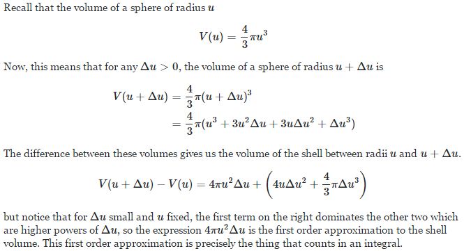
 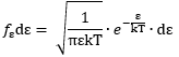 This holds true for any number of degrees of freedom. For example, a diatomic molecule will have extra degrees of freedom, which are related to its rotational and vibrational motion (I explained that in my June-July 2015 posts too, so please go there if you’d want to know more). So we can really use this stuff in, for example, the theory of the specific heat of gases. 🙂

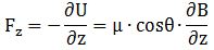
 Of course, we may already note that, in quantum mechanics, Umag will only take on a very limited set of values. To be precise, for a particle with spin number j = 1/2, the possible values of Umag will be limited to two values only. We will come back to that in a moment. First that force formula.


 The μ in this formula is the magnitude of the magnetic moment of the individual atoms and so… Well… It’s just like the formula for the electric polarization P, which we described in


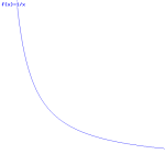


 As Feynman writes, all of the wave functions approach zero rapidly for large r (also, confusingly, denoted as ρ) after oscillating a few times, with the number of ‘bumps’ equal to n. Of course, you should note that you should put the time factor back in in order to correctly interpret these functions. Indeed, remember how we separated them when we wrote:
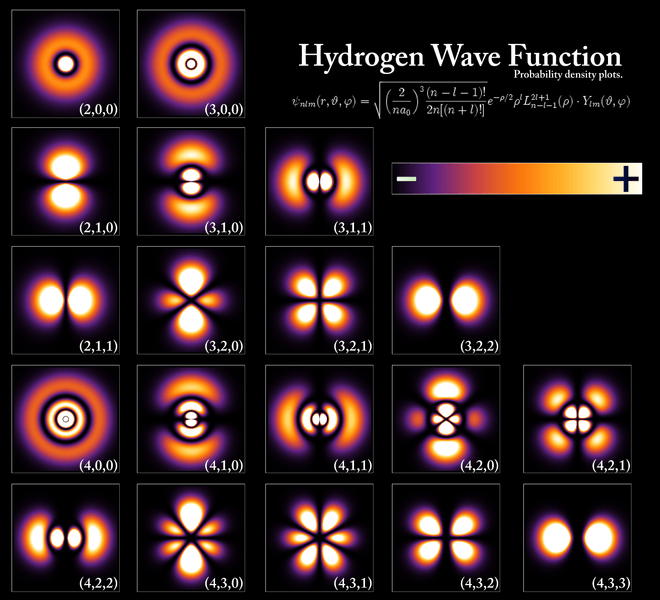
 First, the function is being inverted, so we go from y = f(x) to x = g(y) with g = f−1. In this case, we know that if y = sin(6x) + 2 (that’s the function above), then x = (1/6)·arcsin(y – 2). [Note the troublesome convention to denote the inverse function by the -1 superscript: it’s troublesome because that superscript is also used for a reciprocal—and f−1 has, obviously, nothing to do with 1/f. In any case, let’s move on.] So we swap the x-axis for the y-axis, and vice versa. In fact, to be precise, we reflect them about the diagonal. In fact, w’re reflecting the whole space here, including the graph of the function. Note that, in three-dimensional space, this reflection can also be looked at as a rotation – again, of all space, including the graph and the axes – by 180 degrees. The axis of rotation is, obviously, the same diagonal. [I like how the animation visualizes this. Neat! It made me think!]
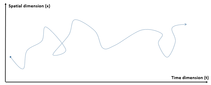
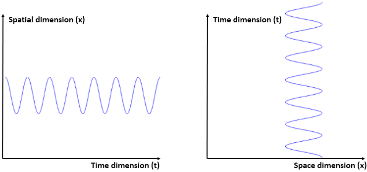
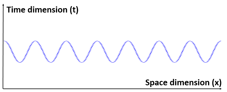
 Now think of wrapping that around some circle. We’d get something like below. [Don’t worry about the precise shape of the graph, as I made up a new one. Note the remark on the need to have a well-behaved function applies here too!]
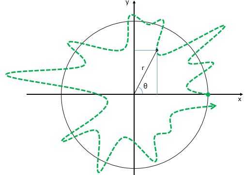 Neat, you’ll say, but so what? All we’ve done so far is show that we can represent some itinerary in spacetime in two different ways. In the first representation, we measure time along some linear axis, while, in the second representation, time becomes some angle—an angle that increases, counter-clockwise. To put it differently: time becomes an angular velocity.
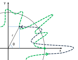


